N90-24367

Experiments and Other Methods for Developing Expertise

with Design of Experiments in a Classroom Setting

John W. Patterson

lowa State University

Ames, Iowa

INTRODUCTION

The only way to gain genuine expertise in "SPC" (Statistical Process Control)

and "DOX" (the design of experiments) is with repeated practice, but not on

canned problems with "dead" data sets. Rather, one must negotiate a wide variety

of problems each with its own peculiarities and its own constantly changing data.

The problems should not be of the type for which there is a single, well-defined

answer that can be looked up in a fraternity file or in some text. The problems

should match as closely as possible the open-ended types for which there is always

an abundance of uncertainty. These are the only kinds that arise in real research,

whether that be basic research in academe or engineering research in industry.

To gain this kind of experience, either as a professional consultant or as an

industrial employee, takes years. Vast amounts of money, not to mention careers,

must be put at risk. The purpose here is to outline some realistic simulation-type

lab exercises that are so simple and inexpensive to run that the students can

repeat them as often as desired at virtually no cost. Simulations also allow the

instructor to design problems whose outcomes are as noisy as desired but still

predictable within limits. Also the instructor and the students can learn a great

deal more from the postmortumconducted after the exercise is completed. One

never knows for sure what the "true data" should have been when dealing only with

"real life" experiments. To add a bit more realism to the exercises it is some-

times desirable to make the students pay for each experimental result from a make-

believe budget allocation for the problem.

Of course, the students find all this open-endedness and uncertainty very

unsettling, but this is what most characterizes the kinds of investigations they

will encounter later and it is important that these features be part of the

students' lab experience. Better that the students' first encounters with these

kinds of anxieties come in a college classroom under the tutelage of an experi-

enced educator, than on their first job under the direction of a stressed out

supervisor.

MECHANICAL SIMULATION

To be most effective, a lab exercise should be mechanical in nature and

completely open to visual inspection while it is working. The reason is simple:

_ii our experience is at the macroscopic level where mechanical phenomena dominate

and it is largely by "seeing" that we have gained our experience. Hence, we take

119

PRECED|NG PAGE BLANK NOT FILMED

https://ntrs.nasa.gov/search.jsp?R=19900015051 2018-07-16T19:36:29+00:00Z

data points more seriously when we can plainly see them being generated in a

simple, easily understood fashion. Only later should one go to more exotic data

production schemes, such as analog circuits or computers whose inner workings are

usually much further removed from the world we experience.

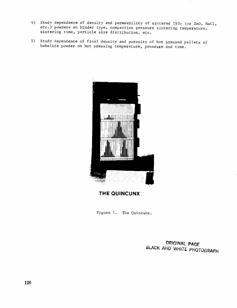
One of the most effective teaching devices for introducing students to

statistical methods is the so-called Quincunx, originally introduced by Sir Francis

Galton back in the 1800's (see Figure i). These simple machines allow one to

generate endless sequences of samples, each drawn from a well defined population

of known mean and standard deviation. Even easier to understand are the sampling

boxes and sampling bowl schemes that are also in wide use today (see Figures 2-4).

None of these are difficult to construct, but all are commercially available. For

example, the Lightning Calculator Company of Troy, Michigan ([313]-649-4462) sells

ready-to-use versions of the Quincunx, chip boxes, sampling boxes, and sampling

bowls. They come completely assembled and are shipped with brief instructional

brochures, an audio cassette, and ready-to-copy data forms for use in the lab.

Statco Products, also of Troy, Michigan ([313]-879-7224)offers a similar array ofsuch items.

Xbar-R charts for in-control processes are easily constructed using these

devices and the students benefit from seeing the histograms take shape as the beads

are dropped. Attributes charts (% defective, etc.) are best illustrated by

sampling from a mixture of differently colored beads all housed in the same bowl.

Specially constructed paddles make it easy to draw samples of various sizes.

Sampling bowls can be used to construct and study p charts, u charts and c charts.

To control the attribute's mean frequency (% defective etc.), one simply

adjusts the fraction of beads having a particular color in the sampling bowl. To

examine the effects of different sample sizes one simply uses a different sampling

paddle. With the quincunx, one controls the location of the bead drop by sliding

it left or right. Different pegboards can be inserted to change the standard

deviation of the Quincunx and the user decides on the number of beads dropped per

sample. Again, the ease of operation of sampling bowls and the Quincunx makes it

possible for the students to conduct as many runs as they care to and the data

generation procedure is not nearly the time consuming distraction it is when actual

experiments are used. Sometimes students dream up personal mini-research

investigations to check various aspects of the recommended SPC and DOX procedures.

Consider, for example, a scatter diagram study of the relation between the ranges

and standard deviation of samples drawn from a Quincunx. Will the relation depend

on the number of items per sample? Could this kind of information be used to

convert R bar values into control limits on an Xbar-R chart? The possibilities

are almost endless.

Also available from the Lightning Calculator people is a process simulation

training kit called "prosim" (See Figure 5). It explains how the Quincunx can be

used to demonstrate such statistical design strategies as One Way ANOVA, 22 and 23

factorial designs, two factor expriments with interactions, and Taguchi's Ls and

L90rthogonal Arrays. After a little thought, however, it is easy to see how these

instructions could be modified so as to simulate data for almost any kind of

statistical design strategy in use today, including the so-called response surface

methods.

120

COMPUTER SIMULATION

Once you see how the mechanical simulators work, it is a fairly simple matter

to write programs that do the same thing either on a PC or on a hand held program-

mable calcblator. Two software packages, a statistics simulator and an SPC

simulator, were described in pp 84-5 of the July 1989 Quality Progress. In

essence, they are computer versions of the Quincunx and run on IBM/PC/XT/AT

compatibles having 128K of memory and one or more disk drives.

In my view, computer simulation methods are most useful for teaching and

learning the strategies for designing multi-factor experiments and then interpret-

ing the results. Many people insist that only real life experiments carried out

with actual laboratory equipment should be used when teaching the design of

experiments; however, I disagree. Restricting oneself only to real life

experiments of the simplest sort, there is no definitive way to critically check

the inferences one is led to with the DOX strategies he or she is employing. And

if one tries to solve this problem by going to a very simple experiment--such as

studying the period of a simple pendulum as a function of the mass, length and

starting angle of the pendulum--the students simply go to the closest physics

text to see what dependences are predicted from theory. This eliminates the most

important aspect of the exercise, namely the haunting feeling one has about

investigating some response variable without knowing whether--much less how--it

depends on the controls being studied. Knowing these things beforehand completely

changes the mindset of the investigator and can severely undermine his or her

ability to proceed objectively.

By using tailor-made simulation programs, the instructor can generate noisy

data from a well understood law such as the gas law, V = nRT/P. But the law

should then be disguised by replacing V, n, T and P with Y, u, v and w respectively.

Also, by adding a superfluous control variable or two, say x and z, (that do not

appear in the gas law formula), the instructor knows to look for these as being

totally insignificant factors in the experiment. If they do register significant

effects, either the student or the DOX software must be doing something wrong.

Afterwards, the students can be told that Y was really the volume of a perfect

gas, u was the number of moles, v the absolute temperature, w the pressure and

that x and z were dummy variables all along. When all this is revealed afterwards,

the students find "the scales falling from their eyes", so to speak, and can then

review the decisions they made in a totally different light, namely that of

informed hindsight.

Here in un__disguised form is a DOX problem based on the gas law. Shown in

Figure 7 is the computer code I used to simulate noisy V data on a Casio fx-80OOG

(or fx-7000 G) hand held programmable calculator.

HANDS-ON, IN CLASS EXERCISE USING SIMULATED DATA

Design, execute and interpret an experiment to study the alleged dependence

of gas volume (V:I0 350)* on mole number (n:0.5 2.0), temperature (T:300 i000),

*The values over which the variables are to be ranged are bracketed by the numeri-

cal values following the colon. The same is true for the control variables n, T

and P.

121

pressure (P:O.5 2.0), and xylene content (x:0.01.0). Assumewe require a resolutionof 1.5 units for the response variable V and that its estimated standard deviationis about 0.7.

Steps: i) Execute the resolution preliminaries.

2) Design an experiment using a linear, factorial, quadratic or cubic

design for all four of the control variables listed above (n,T,P,x).

Use five replications.

3) Conduct experiments at the control settings given your experimental

design and analyze the data.

4) Produce an effects table and analyze it to see if any of the four

control factors has little or no effect.

5) Produce contour maps of P vs T for n = 0.5 and 1.25 and shade in the

P-T domain(s) for which V is less than 50 but greater than 30,

6) Now use the ideal gas law to sketch in the "true" contours for V = 50

(or any other choice that meets your fancy) and compare these to the

same contours on the response surface map.

In the MSE 341 course at Iowa State, we use a software package called EChip to

teach expertise in experimental design. This will be described further below. The

following problem is taken directly from the EChip text and the software contains

a simulator program that can generate response data for whatever control variable

settings the user wishes to specify. I include here the entire problem description

but not the simulator program nor the extended text discussion of the problem.

However, I think the reader will appreciate the realistic nature of the problem,

which is based on an industrial problem that was successfully solved by an EChip

user.

ECHIP PROBLEM 5: EXTRUSION OF A NEW THERMOPLASTIC

This is a wrap-up problem that ties together all you have learned so far.

should take about four hours to complete and everyone should be able to obtain

a defensible solution using the methods discussed thus far.

It

Background

You work in R and D in the plastics division and have been asked to fully

define the process for making a new plastic in one of the extruders on the compound-

ing line. An extruder is like a giant meat grinder with a massive internal screw

(auger) in the extended barrel. Raw materials are fed into the receiving funnel

at one end; these are melted and mixed by a combination of heat added by elements

on the barrel wall and by the shearing action of the auger. Everything eventually

gets pumped out the extruder die (hole) at the exit end of the barrel.

122

The Control Variables

On talking with the inventor of the new plastic, you find he has worked only

with small, lab scale equipment and that he has not defined the precise viscosity

of the base polymer of the new plastic. Consequently, you will have to determine

the percentage of the two additives add i and add 2. He also says that the mois-

ture content of the base polymer (which you can control) often seems to be

important.

You can control the temperature in each of four zones along the extruder

barrel (TI,T2,T3 and T4) by automatic controllers on the heater elements.

Adding all this to information obtained from the operators of the extruder,

you find there are at least ten control variables that may or not be important.

Here they are along with the ranges over which they can be adjusted.

Add 1.... 0.0% to 0.5%. This is supposed to induce uniform melting.

Add 2... 2.0% to 4.0%. This is a filler that is said to improve strength.

Viscosity... The viscosity can be set anywhere from 60 to 80.Moisture... The moisture content can be set from 0.1% to 0.25%.

TI through T_...Each can be controlled at 260C min to 320C max, independently.

Rate... Feed rate of input is from i00 to 200 pounds/hr.

RPM (auger)..Can be set anywhere from 150 to 300 rpm.

The Response Variables

On talking to your marketing people, you conclude that tensile strength (TS)

is the most important property but measuring it requires a destructive test. It

would be nice if the TS correlated with some easily monitored manufacturing

variables so that the TS for each batch could be estimated from the other measurable

variable. Old hands tell you they can pretty well estimate the TS of thermoplastics

from the temperature of the melt during production. This is almost too good to be

true so you decide to verify their claim by studying both the TS and the melt T as

response variables. So your responses are chosen as follows.

Estimated range is from 280 to 325C

Ranges from 15000 psi to 30,000 psi with the minimum advertised

specification being 25000 psi

Standard Deviation and Resolution

Discussions with marketing have resulted in a desired resolution of 10%. The

general argument is that products less than 22,500 psi will be totally unacceptable.

Since this is 10% less than 25,000 psi, the resolution of the experiment must be

capable of detecting at least this difference.

You are fortunate in having a data base of tensile testing data from which you

have calculated a standard deviation estimate of 0.02 for log 10 tensile strength.

The antilog of 0.02 is approximately 1.05 which means that the standard deviation

is about half of the desired resolution.

You may use 0.04 (the common log of (1.10) for resolution and 0.02 for standard

deviation in the number of trials calculations.

123

Final Hints

Make sure you have the goals clear. Many students, proceeding in haste, think

optimization is the only goal. If you think this, reread p 5.4 very carefully.

Check it out. Try your model out and see how well it predicts.

All of the indicators may be positive. There may be no lack of fit indicated

in the Effects Table, and the contour plots may make sense, but the model may still

be in error. There is little redundancy in the recommended designs and they can

fit the particular set of data but not the response surface from which the data

comes; recording errors are a common problem.

The comments about the analysis of linear designs in the last paragraph of

section 10.2 are important.

This problem should be worked several times. The first time without using

design augmentation. Get fresh data at each stage. Once you have "solved" it this

way and read Appendix B, you can redo it with design augmentation. For a third

trial, you might try blocking-- once without blocking is recommended.

ECHIP'S DOX SOFTWARE

Many factors have conspired to keep undergraduate engineers from gaining

knowledge of the DOX strategies they so badly need. For example, few if any

engineering students have had the time or inclination to fulfill the prerequisites

required for the DOX courses traditionally offered in statistics departments. This

has tended to keep them out of formal DOX courses in college. Those engineers who

have learned these methods have done so either as part of a graduate program or,

more likely, by attending intensive short courses after graduation and at some

employer's expense. Such short courses are marketed by numerous companies, consul-

tants and continuing education units around the country. Interestingly, they

learned to use DOX without taking all the traditional prerequisites. Also, more

and more software packages with DOX capabilities are becoming available to the

users of personal computers and these, too, can be used quite effectively by students

_o have not taken extensive prerequisite courses in statistics. In other words,

engineers are bypassing departments of statistics and are learning DOX strategies

on the job, either from short courses or through the use of software packages or

both.

In an effort to better prepare our MSE students for what they will face upon

graduation, we have purchased a license to use the EChip software package in our

MSE 341 course. We feel its statistical methods are more than rigorous enough for

our purposes and we especially appreciate EChip's emphasis on strategies rather than

statistics or calculation procedures. The software focuses more on how to make the

key decisions when designing and executing experiments and leaves the computational

details and statistical analyses to the computer and keeps them "behind the scenes",

as it were. After first deciding whether the proposed investigation will fit within

the available budget, the user is directed on a swift but systematic course of

action through the cycle shown in Fig. 8. An extensive array of response surfaces

produced in the form of contour maps that can be scrolled, sorted through and

124

interacted with in the most useful fashion. Upon completion of the study, one

decides on whether or not another battery of experiments should be undertaken.

so, the procedure is repeated, though in a modified form that accounts for what

has been learned or what variables may be left out.

If

EChip provides a choice of several standard designs plus a powerful algorithmic

design option for use when none of the standard ones can possibly suffice. This

can occur when certain regions of the control variable space simply cannot be

sampled due to unavoidable technical difficulties. EChip enables the user to

disallow whole groups of troublesome control variable settings and then to

algorithmically devise an optimal design in the subregion of settings that is

left. Algorithmic designs are also used when mixture variables are to be included

or when one wishes to augment the design executed in the previous iteration.

As EChip is response surface oriented, the response variables (several may be

studied simultaneously) must be of the continuous type. Some but not all the

controls may be of the categorical variety but the software is intended for studies

involving continuous control variables for the most part. EChip's ability to

handle both mixture and nonmixture controls simultaneously makes it especially

useful for materials and chemical engineers.

CONCLUDING REMARKS

In the foregoing s_ctions, I have promoted the use of simulation schemes,

first of the mechanical-visual sorts and later of the computer-numerical types.

In my view, these are the best ways to generate response data for multifactor

experiments. Since the instructor specifies everything (including the noise

level!) in the model that generates the data, it is relatively easy to diagnose

the mistakes that arise in the students' work because there is no possibility

for poor lab methods or experimental equipment failures to cause problems.

Discrepancies can only be due either to software bugs or to inadequacies in the

DOX strategies being used or to mistakes or poor judgment by the user. I, for

one, very much favor the simulation approach when trying to help students acquire

expertise in the use of DOX methods for analyzing or optimizing complicated multi-

factor processes. On the other hand there is indeed a lot to be said for also

including real experiments in such a course, despite all the difficulties they

may entail. For this reason, I conclude by citing a number of candidate experi-

ments we are hoping to incorporate in the MSE 341 course in future offerings.

Unlike the examples discussed so far, these place much greater emphasis on mixture

variables.

i) Study the dependence of AC conductance and capacitance for aqueous solutions

(H20 + NaCI + sugar + H2CO3 + etc.) on temperature (°K) compositions (mixture

variables), AC frequency (H2), geometric variables (distance between elec-

trodes, their areas, etc.).

2) Study AC conductance, capacitance and density of moist soils (H20 + sand,

silt, etc.) and their dependences on compaction pressure, water contact,

soil type, AC frequency, etc.

3) Study dependence of freezing point depression of aqueous (or other) solutions

on composition variables.

125

4)

5)

Study dependence of density and permeability of sintered Ti02 (or ZnO, NaCI,

etc.) powders on binder type, compaction pressure sintering temperature,

sintering time, particle size distribution, etc.

Study dependence of final density and porosity of hot pressed pellets of

bakelite powder on hot pressing temperature, pressure and time.

THE QUINCUNX

Figure I. The Quincunx.

ORIGrNAL PAGE

@LACK AND WHITE PHOTOGRAPH

126

Front

Back

THE SAMPLING BOX

Figure 2. The sampling box.

ORIGTN_L- P/tCEBLACK Ah'D Wr_;T_. F_",

ORIGINAL PAGE IS

OF POOR QUALITY 127

THE SAMPLING BOWL

Figure 3. The sampling bowl.

THE CHIP BOX

Figure 4. The chip box.

128

PROSIM, which stands for process simulator, is a training aid that uses aquincunx to teach designed experiments.

The PROSIM kit includes :

• Master Forms to be used by the instructor and student.

• Overhead Masters for instruction and demonstrations.

• A "D" ring binder for the 140 plus page manual.

The training package includes step by step procedures for how to set up anyquincunx with a variety of factors and degrees of significance. The handy setupforms and work sheets will help simplify any design experiment class. The dataanalysis forms included treat conventional designed experiments and TaguchiOrthogonal Arrays.

The detailed procedures included with PROSIM address the followingtopics:

1. How to set up and scale the quincunx.

2. One way ANOVA.

3.2 2 Full Factorial Designs.

4. 23 Full Factorial Designs.

5. Two factor experiments with interactions.

6. Taguchi L80rthogonal Arrays.

7. Taguchi I_90rthogonal Arrays.

PROSIM

Figure 5. Prosim.

ORIGINAL PAGE IS

OF POOR QUALFF(

129

Two Quincunxesfor the PC

................. I ...........

iiiiiiii!iiiiiiiiiiiiiii!iiiiiiiii!ii!iiiiii!i!i!i!ii!iiiiiiiiiiii,-//i _X-14+/+/-X+X+ +IX+I.I .... i

I....... I........................._iii_i!ii_ill iiiiiiiiiiiii:ii:ii!i_i_i_i i i iilii!_i_i!i;i;iiiiiiii i!iii ii!ii il i_! i!iii_iiii_i i_iiii!iiii!_i_:! ii!i_iliiii_i_!i iilliiiiiiii!i_

i!i i!i !_i!i!! iiiil!iiiiii!ili_ _

l ...... ,:.e ............. ....

SIMULATOR I_* _1ove So%n-oel1-8 Drop B&lls I

F! Speec{ Do_n ]F2 Speec_ Up I:3 l_az'r o_er [:4 Wi_erF: S_a1:*s¢:c$ ]:6 Marker:? 0bsc_zre [

F8 ToI_ S%Op:8 Clear

:I0 QUIT

POSITION 1. g

# Balls 122Hlan I_1. 97Range Iil. 8

Sl_eed mSprIad m

STQTISTICS

FI Line C:_r_eF2 _olid C_rveF3 1_ean:4 S%d _a_, "

F5 P.-Oba_Cll:_yF: :IaZ"Ize.-F 9 BallsiF8 SaveIF3 Clear

[F!O OUIT

POSITION 1 ,

l Balls 12_Mian cl. 97Range @. 8SOd Dev e..I.7

Speed iSPread

This zSme oeaO frame _n tree Statistics SImuJator IIS_nOWS a sample

of 120 cenlerec or_ 1 The s_ancard oeviallon can oe varleO by using the

_3 anc F4 Keys LJoDer arlo lower soec hmtts were otawrl Tn using _he F6

Key

This IS _he StaI_stlcs SlmulatOr arlalvsls screen Dasec on the .1-

|ormaIlorl in Figure ! Plus arlc minus $tarloaro Qevla_lor_ i[rl_s a!sc carl

De orawn in. ano trle _roportlOrl Detween any two iImlls can Q9 ca!cu:a[ec

........... [u .......... X B_R CH_RT

...... ''.'.'-'.'.'-''"-"".'..-:"." ". '-" _" :_o¢ < > Spe_d I

::::::::::::::::::::::::::::::::::: F3 Range _4 Bo_h.................. IF_m_o :?s=alzl

I............. :. ::: : :: : ::: :: : :: :: ::i::8 ::'tu_, I

: ......... X I. _2t r., J_1.41.31.2I.I

8.9

_.?8.6

UCLR

LCL

a.43

0,8 I"

-0.5

_'_ .... ' " C ..........._"S'* "I--0:_ _ ................... LCL_

:l _,_le 1 _z _, _ -u = LCL F3 P..... le F5 R .....

The Stal!stcal Process Corltrc_ Simu ator OrQOuCes an X-par cnan

w,m hmrts trial can De up,area "he effect of ao_ustrng the mean 3Drea_

or DOln can De demonsttale_ eas W

Pressimg tDe F5 Key CiSOlavs tr_e ",<.oar ana ranae crlacs Merlu

se!ector1s are always vrSlDle Cn _r_e screen n 1_e _taI]st_ca! c_rcgess Con-trol Simulator

Figure 6. Two Quincunxes for the PC

Figure 6 reprinted with permission, Quality Progress, July 1988

130ORIGINAL PAGE IS

OF POOR QUALITY

PROG 5 Comments and Remarks

Mcl

"SD"?_S

Lbl i

PROG 3

"n" ?-+N

"T" ?-+T

,,p,,?_p

"x" ?-+x

.082NT + P_V

V + S x A_V

"V=" :V A

GOTO I

(CASIO fx-7000G)

PROG 3

_A'48_F:LbI2

A + RAN#_A

DS2 F:GOTO 2

(A-24) + 2_A

(CASIO fx-7000G)

Clears all memory registers

Prompts for STD. DEV. "(TRUE)" and stores it in S

PROG 3 is a subroutine that returns a number

"A" drawn from a normal (0.i) population

Prompts for a value of n and stores it in reg. N

" " " " " T " " " " " T

,, ,, ,, ,, ,, p ,, ,, ,, ,, ,, p

It ,T ti Vl ,, X It V, ,! 1, It X

Calculates the "TRUE" value of V and stores it in

Adds a normal residual noise contribution (STD

DEV = S) onto V(TRUE) and stores that in V

Displays V = and the value just simulated

cycles back to Lbl 1 for the next simulated

experimental result

Comments and Remarks

Sets A to _ and counter, F, to 48

Adds RAN# (uniform in int. 0-i) to register A

Decreases counter By 1.0 when F > %, GOTO Lbl2

When F drops to _, convert the sum in

A to a normal (0,i) value and store it in

A for use in the main program.

V

Figure 7. A program with subroutine for simulating volume data

with a known variability. Assumes V = _RT/P.

The Experimental Cycle

WRITEREPORT

STUDY THE

CONTOUR PLOT

DECIDE ON• RESOLUTION

CONSULTAN

EXPERT

CHOOSEVARIABLES

L

DESIGN

EXPERIMENT 's

ANALYZE

DATA

RUN ",l

EXPERIMENT ;

ENTER DATA

Figure 8.

131