N90-19406

1989

NASA/ASEE SUMMER FACULTY FELLOWSHIP PROGRAM

MARSHALL SPACE FLIGHT CENTER

THE UNIVERSITY OF ALABAMA IN HUNTSVILLE

INVESTIGATIONS INTO A NEW ALGORITHM FOR CALCULATING

H ® OPTIMAL CONTROLLERS

Prepared by:

Academic Rank:

University and Department:

R. Dennis Irwin

Assistant Professor

Ohio University

Department of Electrical

and Computer Engineering

NASA/MSFC:

Laboratory:Division:

Branch:

MSFC Colleague:

Date:

Contract:

Structures and Dynamics

Control Systems

Pointing Control Systems

Henry Waites

August 31, 1989

The University of Alabamain Huntsville

NGT 01-008-021

XVI

ORIGINAL _' _- .r':-L:h:. _"

OF POOR QUAL_]¥

https://ntrs.nasa.gov/search.jsp?R=19900010090 2018-07-09T14:54:12+00:00Z

INVESTIGATIONS INTO A NEW ALGORITHM FOR CALCULATING

H" OPTIMAL CONTROLLERS

by

R. Dennis Irwin

Assistant Professor of Electrical and Computer Engineering

Ohio University

Athens, Ohio

ABSTRACT

A new algorithm for calculating H" optimal controllers

is investigated. The new algorithm is significantly simpler

than existing approaches and yields much simpler

controllers. The design equations are first presented.

Special system transformations required to apply the new

algorithm are then presented. The use of the new algorithm

with sampled-data systems is outlined in detail.

Several constraints on the characteristics of the

problem formulation are required for the application of the

design equations. The consequences of these constraints are

investigated by applying the algorithm to a simplified

design for a subsystem of a large space structure ground

test facility. The investigation of these constraints is

continued by application of the design equations and

constraints to an extremely simple tracking problem. The

result of these investigations is the development of a

frequency dependent weighting strategy that allows realistic

control problems to be cast in a form compatible with the

new algorithm.

Further work is indicated in the area of developing

strategies for choosing frequency-dependent weights to

achieve specific design goals. The use of the freedom in

problem formulation to achieve robustness/performance

tradeoffs should also be investigated.

It is not clear that the new algorithm always leads to

simpler controllers. The more restrictive formulation may

dictate that frequency-dependent weighting adds to the

controller order disproportionately. This effect must also

be investigated.

XVI - i

groin(A)

Om_ ×(A)

II

IMC

BET

LOS

LQG

Iio

NOMENCLATURE

minimum singular value of a matrix A

maximum singular value of a matrix A

infinity norm of a system transfer functionmatrix

image motion compensation

base excitation table

line of sight

linear-quadratic Gaussian

XVI - iiQ

INTRODUCTION

Until the recent work by Glover and Doyle [I], the design

of H _ controllers promised to be a long and arduous ordeal

for the designer. Moreover, the resulting controllers

tended to be extremely complex, sometimes exceeding the

order of the control model by a factor of five. Their

publication of design equations for controllers of the same

order as the control model is thus a significant advance in

the state of the art. However, the question of whether H ®

control techniques can be successfully applied to large

spnce structure (LSS) control design problems is by no meansanswered.

The foremost question in the mind of any LSS control

designer is that of applicability of H _ techniques to the

usual goals of LSS control. It is known that H ®

optimization can achieve (at least mathematically) any of

the goals of disturbance rejection, command tracking, and

robustness. What is not known is whether H ® design methods

can be used to design controllers which simultaneously give

acceptable performance and do not suffer from the known

shortcomings of LQG techniques, e.g., lack of robustness.

The purpose of the work presented here is to address the

issues of the applicability of the new algorithm for

calculating H_ controllers for large space structures.

The organization of the report is as follows. Section

1.0 contains a brief discussion of the H ® performance

criterion and the design equations which must be solved in

order to find the optimal H ® controller.

Section 2.0 describes a transformation required to

satisfy constraints on using the design equations. The

result is a set of equations that can be readily used to

transform a given state space realization to one of the

required form.

Section 3.0 outlines modifications to the state space

formulation that are required in order to apply H" design

formulas to sampled data systems. The result is a set of

state space formulas for applying the well known w-plane

transformation to multivariable control problems. The L-_]

equations, minus the derivation, can be found in Glover. An

outline of the derivation is included here for completeness.

v

XVI - 1

Section 4.0 documents the application of H" techniquesto a simplified model of the ACES IMC subsystem, includingBET disturbance effects. Section 5.0 uses a simple trackingproblem to discuss weighting schemes which allow the newalgorithm to be applied to realistic control designproblems.

Section 6.0 contains conclusions and recommendationsfor further work. In particular, it is suggested thatstrategies for developing frequency-dependent weights beinvestigated.

1.0 H® PERFORMANCE CRITERION AND DESIGN EQUATIONS

The H _ control problem can be stated as follows.

system equations are

The

= Ax + B1w + B2u

z = C1x + D11w + D12u

y = C2x + D21w + D22u

where w is in R ml, u is in R _, z is in R PI, and y is in R _.

The signal w is an exogenous input which may be either

disturbances or command signals; u is the control input

vector; z is actually the performance related vector; and y

is the vector of measurements that is actually available forfeedback.

Although most calculations with this technique are done

in state space form, the performance criterion is most

easily stated in the frequency domain in terms of the closed

loop transfer function matrix. The open loop transfer

function matrix can be expressed in terms of appropriate

partitions as

G11(s ) = [A, BI, CI, D11 ]

G12(s) = [A, B2, CI, D12 ]

XVI - 2

G21(s) = [A, BI, C2, D21]

G22(S) = [A, B2, C2, D22 ] .

If a controller with transfer function matrix K(s) is

connected from y to u, the closed loop transfer function

matrix is given by

T(s) = G11 + GI2K(I - G22K)IG21 .

The H ® control problem is to find a controller K which

yields a stable closed loop system and for a prespecified

real number F,

II T < r

where

I ] T I I. : sup Oma×(T(jw)).

In the special case of a scalar transfer function, the goal

can be stated as simply insuring that the closed loop

frequency response has a magnitude less than F. This is

clearly important in disturbance rejection problems and can

be used also for tracking type problems.

The }{_ optimal control problem is that of finding the

smallest such F such that a stabilizing controller exists.

Note that once a method of satisfying a given F bound is

identified, the job of obtaining an optimal solution is not

difficult, although it is iterative. The significance of

the recent work of Glover and Doyle is that their equations

yield not only a controller that achieves the prespecified

bound but is only the order of the original control model.

The original factorization algorithms tended to yield

controllers many times as large as the original plant.

Several constraints must be placed on the plant

equations in order to apply the design equations. The first

constraint is that the realization (A, B2, C2) be

XVI - 3

stabilizable and detectable, as is usual.

The second constraint is actually two constraints thatare artifacts of the derivation procedure and are requiredfor well-posedness. They are

rank D12= m2

and

rank D21= P2"

One of the consequences of the above rank conditions is thatthe control input u must appear in the performance orientedregulated variable z. This condition is similar to acondition required for well posedness of the LQG problem.These conditions also insure the calculation of a realizablecontroller. It will also be seen in subsequent sectionsthat these requirements cause some difficulty in calculatinga low order controller.

An assumption which is not independent of the aboverank conditions is that

T

D12 = [0 I]

and

D21 = [0 I].

Transformations to achieve the required forms for D12 and D21will be derived later.

The final constraints are necessary for the design

equations to yield a solution. They are not necessary in

the strict sense. However, it is not known how to calculatecontrollers to achieve the bound when these conditions are

violated. Sufficient conditions for the design equations towork are

XVI - 4

The realizations of G12and G21are minimal.

rank GI2(Jw) = m 2 for all w

and

rank G21(Jw) : P2 for all w.

The design equations can be presented in an abbreviated

form by denoting the solution to the Riccati equation

Q + XA + ATX - XPX = 0

by its Hamiltonian matrix

X : Ric

[)I_ is also partitioned as

D11 :i Dl1121

Dl111

LDl121 Dl122

Two intermediate variables are defined:

Dlx : [D11 DI2]

l)xl [ D T T: 1_ DT12]

Then define

XVI - 5

= DxIDTxI -

X= = Ric

where

p = BR IB T, U = A - BRIDTIxC I, and Q = C_iCi - CTIDIxR'IDTIxCI"

Similarly,

Y= = Ric

where now

p = CTR'IC, U = A T - CTR'IDxIBT I, and Q = BIBTI - BIDTxIR'ID×IBTI •

similarly to LQG design, matrices F and H are defined as

F = -R'I[DTIxC I + BTX®] = [FIll FT12 FTz]

XVI - 6

H -- -[BIDT×I + Y=CT]R"I = [H11 H12 H2].

At this point, it is necessary to perform tests todetermine whether it is possible to achieve the specified Fby designing a controller via the design equations. Thefirst test has important practical consequences in terms ofproper problem setup. It involves direct feed through ofthe disturbance input w in terms of D11:

F > maX{Omax[D1111D1112], O_x[DT1111 DT1121]}.

The last test involves the characteristics of the solutions

to the two Riccati equations:

X_ > O

Y_ > O

and

_max(X.Y.) < F, where # is an eigenvalue.

Under the constraints listed and subject to passage of

the tests an n th order stabilizing controller which achieves

the inequality I ITI I= < F is given by

---- DT (r2I - 1)'1Dl112 Dl122Dll -Dl121 1111 D1111DT111 -

D12 and D21 satisfy

DI2DTI2 : I - D1121(F2I - DTII11D1111)'IDT1121 and

DT21D21 : I - DTI112(F2I - DI111DT1111)'1D1112

XVI - 7

from which

B2 = (B2 + H12)D12

C2 = -D21(C 2 + F12 )Z

B I = -H 2 + B2D'112D11

C I = F2Z + DIID'121C2

A : A + HC + B2D-112C1

and

Z = (I - F2Y®X®) "I

An n th order controller which achieves the norm bound is

then given by the realization (A, BI, CI). There exist

other controllers which satisfy the norm bound; however,

they are not necessarily of n th order. The controller

design equations for this case are omitted. These more

complex design equations may be found in Glover and Doyle [I]

2.0 Transformation to the Standard Form

In Section 1.0, it was stated that the use of the

design equations place constraints on the form of D12 and

D21. This section outlines in detail a method for achievingthe required form for these matrices. The first step is to

write them in terms of their singular value decompositions

as is shown for D12:

D12 = [U121 U122][7_12 0]TvTI2

D12 = [U122 O121][0 _12]TvT12

XVI - 8

D_2 = [U_z2 U_2_][0 I]TZ'_zVTIz"

ORIGINAL PAGE iS

OF POOR QUALITY

similarly,

D21 : U21[_]21 0] [V211 V212]

T

D2_ = U2_[O I][Va_7 V2_] •

Ncw let

XI :: 12VT12

X-,, = U_I E-1

L]' _2 == [U122 U121 ]

V'21 : [Vzla Vml]"

i)l:: : []'12[0 I]TxI2

The equations for z and y are

z := ClX + D1_w + D12u

y : C2K + Dp_w + D22 u

q}f

z = C_x + D_w + U'_2[O I]X12

XVI - 9

y = Czx + Xz1[0 I] (V'21) Tw + D22

ORIGINAL Pf_G£' _$

OF POOR QUALITY

OT7

(U' )12Tz = (U, z)TcIx + (U,Iz)TD_IW + [0 I]TX12u

X-121y - X'121C2 x + [0 I] (V'21)Tw + X'I21D22 u"

Letting

z' = (U') _z

U v _-- XI2U

y ' = X-121Y

w' = (V'zl)Tw..4

_ives

I :-- A

D'I = BIV'21

-1B ' = B2X2 12

C' = (U132)TI

D' = (U' lZ) TDI_V'11 21

D' = [O _]12

XVl - iO

C ' : X-121C22

21 [0 I]

D'22 : X'121D22X-112

The significance of the transformation is that the norms of

z and w are preserved. This means that designing a

controller to achieve a particular I ITI I. for the

transformed system is equivalent to designing a controller

to achieve the same goal for the untransformed system, once

the reverse transformation is applied to the controller.

3.0 Modifications for Sampled-Data Systems

More traditional controller design techniques must be

developed separately for sampled-data and continuous-time

systems. Fortunately, this is not necessary for H" designs

due to the fact that the performance criterion has a

relatively simple frequency domain representation. The

approach is equivalent to "w-plane" design for single-input,

single-output systems. The open loop system is assumed to

h,lve the form

x k+]) : Ax(k) + B1w(k ) + B2u(k )

z k) : C1x(k) + D11w(k ) + D12u(k )

y k) =: C2x(k ) + DzlW(k ) + D22u(k ) .

This discrete time representation can be obtained using

standard techniques such as those found in Kuo [3]. The

transfer function matrix is given by

G(z) : D + C(zI - A)IB

where for simplicity B, C, D are appropriate concatenations

of the open loop system matrices. The bilinear transform

XVI - ii

z = 1 + w1 - W

k_

is applied to G(z) to obtain

G(w) = D + C[(I+wI)(I-wI) "I - A]IB

= D + C(I-wI) [w(I+A) - (A-I) ]-IB

= D + C(I-wI) [wI - (I+A)'I(A-I) ]'I(I+A)IB.

Using the identity

[I-wI][wI - (I+A)I(A-I)] °I = -I + [I - (I+A)'I(A[I)]

x [wI - (I+A)"(A-I)] "I

G(w) = D - C(I+A)IB + C(I+A)-I[wI - (I+A)I(A-I)]-I(I+A)-IB

so that the w-plane state space representation of G(w) is

D = D - C(I+A)'IB

C : 2C(I+A)

B : (I+A) "I

A_ = (I+A)'I(A-I) .

The controller is then designed using this representation to

obtain K(w), which is represented as a set of continuous

time state equations with matrices Ak, Bk, Ck, D k. Theinverse transform

w : z - 1

z + 1

XVI - 12

is applied to obtain K(z).transformation are

State space formulas for this

Az = -(Ak+I ) (Ak-I) -I

B z = (I+Az) B k

C z := Ck(l+Ak)

D z = D k + Ck(l+Ak)'IBk.

4.0 Problem Setup for IMC Controller Desiqn

The ACES configuration of the Marshall Space Flight

Center Large Space Structure Ground Test Facility is shown

in schematic form in Figure i. The image motion

compensation (IMC) subsystem is comprised of the line-of-

sight (LOS) detectors and the IMC pointing gimbals. The

base excitation table (BET) is the excitation device.

The natural setup for IMC controller design to minimize

the effects of BET excitation is outlined here. The

equations are obtained from a FEM model of the LSS ACES

ground test facility. The first step in the problem setup

is to define the z, w, y, and u. Since the actuators and

sensors are limited to the IMC components, y and u are the x

and y axis detector signals and pointing gimbal torques,

respectively:

u := [IMC× IMC ]

'/ = [I)ET× DE'P ]T

The disturbance vector is most naturally chosen to be the x

<_nd y ax_s BET excitation table forces:

W = [BET× BETy].

XVI - 13

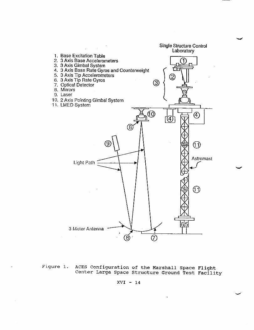
1. Base Excitation Table2. 3 Axis Base Accelerometers

3. 3 Axis Gimbal System4. 3 Axis Base Rate Gyros and Counterweight5. 3 Axis Tip Accelerometers6. 3 Axis Tip Rate Gyros7. Optical Detector8. Mirrors9. Laser

10. 2 Axis Pointing Gimbal System11. LMED System

®

Single Structure ControlLaboratory

!

Light Path

3 Meter Antenna

Astromast

IAk J

®

®

Figure . ACES Configuration of the Marshall SpaceCenter Large Space Structure Ground Test

XVI - 14

Flight

Facility

=

The first elements of the performance oriented controlled

variable vector are

zl = [DET× DETy]T

since the goal of this system is to reduce the displacement

of the line-of-sight of the laser beam from its equilibrium

position on the detector. However, this is not sufficient

to insure that the conditions of the design equations are

met. The additional requirement of control input weighting

is achieved by letting

T

::_ = [IMC x IMCy]

This satisfies the rank condition on D12. The remainder of

the parameters of the problem can be chosen as follows.

B I is comprised of the appropriate modal gains at the BETactuators.

B 2 is comprised of the appropriate modal gains at the IMCactuators.

C I is comprised of the LOS gains at the detector

C 2 is also derived from the LOS gains at the detector.

A] so,

A is in block 2 x 2 diagonal form and

D11 [0 0] T := , DIZ [0 I] T

D21 : 0, D22 = 0.

The design equations still cannot be applied due to the rank

XVI - 15

condition on Dzl. This condition is equivalent to requiringthat the same disturbance enters at two physically separatedpoints in the system. The reason for the condition is amathematical technicality. Unfortunately, it places actualconstraints on the formulation of the problem.

A possible solution to this rank problem is to defineD21to be a very small constant with respect to the norm ofthe transfer function matrix G12at all frequencies ofinterest.

However, it turns out that this is not the onlytheoretical problem with the above formulation. Anotherdifficulty is the minimality condition on the G12realization. The difficulty in the present setup is thatthe requirement is equivalent to the requirement that thedisturbance (in this case the modes ehich can be excited bythe BET) must be controllable at the IMC pointing gimbals.Unfortunately, this is not the case. In fact, the pointinggimbals have significant authority over only four or fivemodes. This is especially troublesome if the technique isused without regard to the minimality condition, as thedesign equations will yield a controller without regard tothe satisfaction of the requirement. In this case, however,the controller will not satisfy the norm bound.

The minimality condition is an artifact of theparticular procedure used to derive the design equations.In the usual factorization approach to H_ control, theminimality condition is not required since it is possible tocarry along completely unrelated realizations for each ofthe four transfer functions matrices. It is interesting tonote that an equivalent requirement for an LQG approachwould be that the disturbance states be controllable as wellas observable.

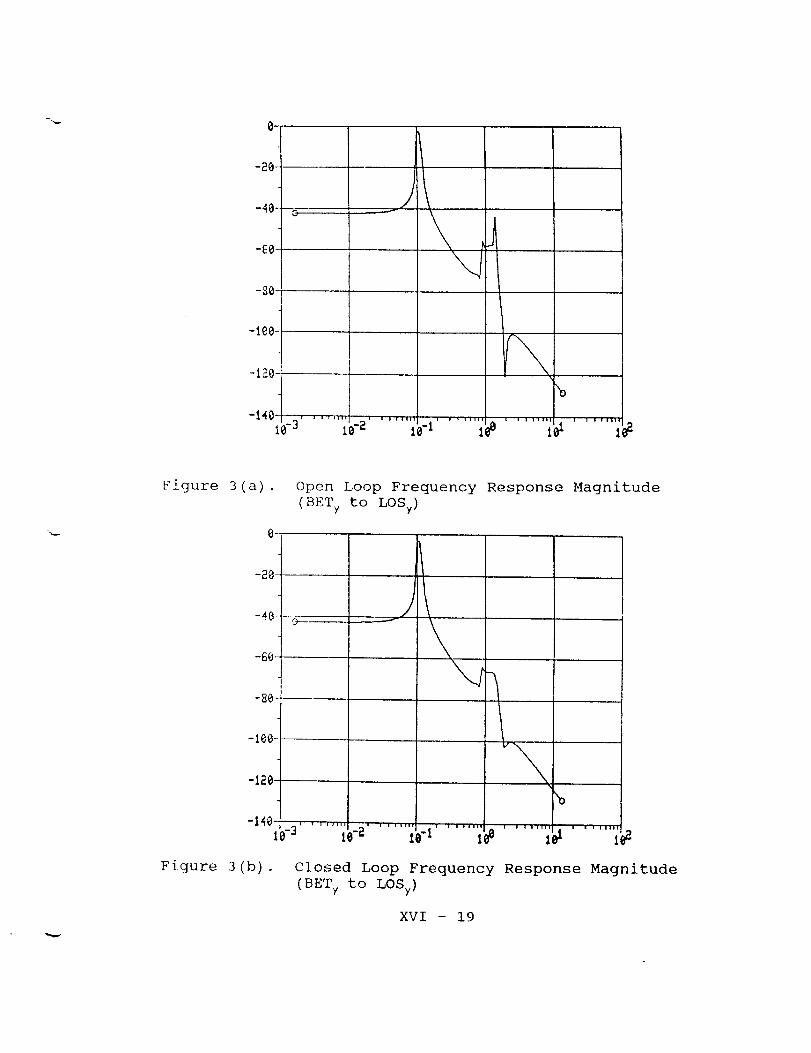
The consequences of violating the minimality conditionare illustrated in Figures 2 and 3. Figure 2(a) is themagnitude of the open loop frequency response from the x-axis BET force input to the x-axis detector. The mode at.15 hertz is the AGS hinge point pendulum mode and isuncontrollable at the IMC gimbals. The other modes arecontrollable. Figure 2(b) is the magnitude of the closed

loop frequency response from the x-axis BET force input to

the x-axis detector. It is apparent that the modes which

are controllable at the IMC gimbals have been effectively

suppressed. However, the AGS hinge point pendulum mode

continues to predominate, although the low frequency

baseline has been reduced. Figure 3 illustrates the fact

XVl - 16

that the closed loop norm is not improved. In Figure 3(a)the open loop frequency response from the y-axis BET forceinput to the y-axis detector has a maximum of roughly -3decibels, as does the closed loop response of Figure 3(b).

In each case, the values are reliable indicators of the

infinity norm, since the the x and y axes are only slightly

coupled. All frequency responses are in transformed

input/output coordinates, as discussed in Section

As these problems were uncovered in the attempt to

obtain an IMC controller design, it was decided to

investigate the properties of the design equations using an

extremely simple model. The next section documents the

findings of this investigation.

XVI - 17

ORIGINAL PAGE !S

OF POOR QUALITY

-10-

-30-'

-40 .....!

i ' //

h

1

I

\\

\

i i ,111, ," i 'l iiil1,!

>o Lei t_

Figure 2(a). Open Loop Frequency Response Magnitude

(BET x to LOS×)

-3_-

Figure 2(b) Closed Loop Frequency Response Magnitude

(BET x to LOSx)

XVI - 18

-_-0-

-4°.-60-

-80iI

-lgO

-120

-140- , ..... _, ,_ ...............Ifa i_a 1o-I I

, l _ i,|)i I ! , i ,i)i_

Figure 3 (a) .

-20-

-4_

-B0,

-80-

-I00-

-120

Figure 3 (b) .

Open Loop Frequency Response Magnitude

(BETy to LOSy)

'o

I ie2

Closed Loop Frequency Response Magnitude

(BETy to LOSy)

XVI - 19

5.0 SIMPLE TRACKING PROBLEM

The usual way to introduce design flexibility in the

factorization approach to H ® optimal control is via

frequency dependent weightings. To see the effect of

frequency dependent weighting, the usual parametrization of

the closed loop transfer function is useful. For a stable

plant, the closed loop transfer function can be written as

q-_l ----- Gll

T 2 = G12

T 3 = G21.

Any stable transfer function Q generates a stable closed

loop transfer function and a controller which achieves that

transfer function. In fact, every stable closed loop

transfer function is generated by some stable Q.

The usual requirement for a solution to exist is that

T z and T 3 have constant rank on the extended jw axis. No

minimality condition is required. Weighting is introduced

by solving the modified problem of minimizing the infinity

norm of

T I - T2W2QW3T 3

where W 2 and W 3 are chosen to satisfy the constant rank

condition and to define frequency ranges over which

optimalit_ is emphasized. The major difference in the

general H- problem and the problem solved by the new design

equations in question is the presence of the two minimality

conditions. The effects of the constraints are most easily

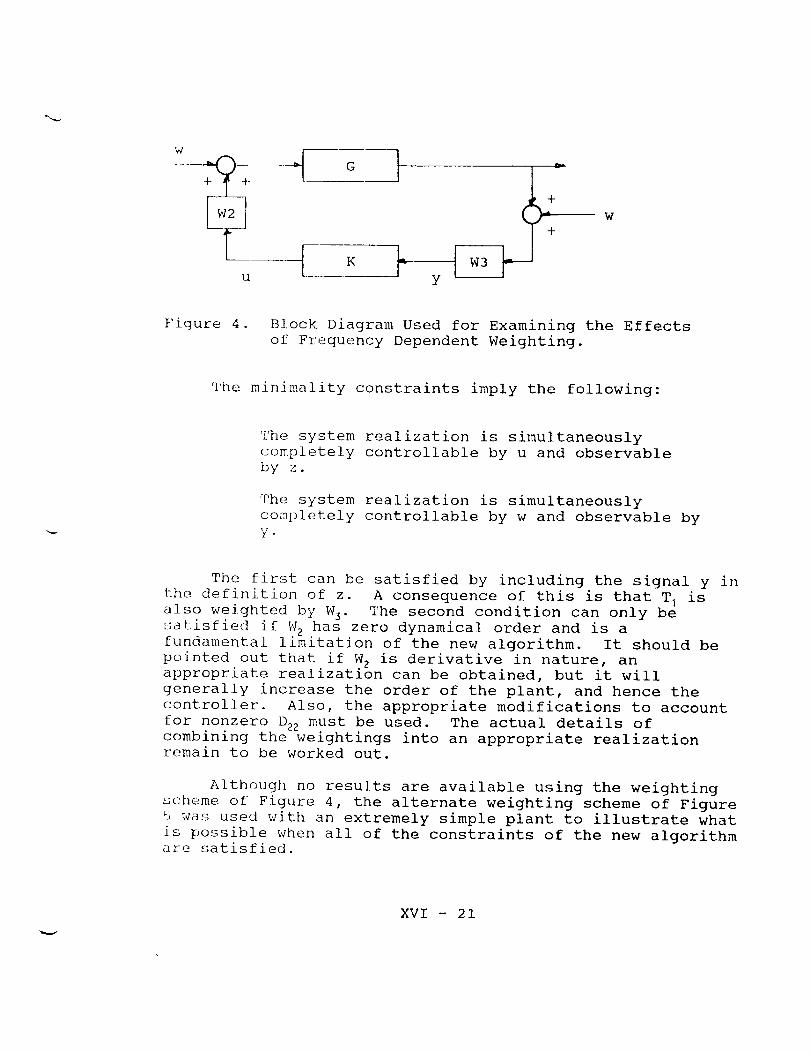
seen by examining the block diagram of Figure 4.

XVI - 20

w

+

U

K

<

Y

+

Figure 4. Block Diagram Used for Examining the Effects

of Frequency Dependent Weighting.

The min]mality constraints imply the following:

The system realization is simultaneously

completely controllable by u and observable

by z.

The system realization is simultaneously

completely controllable by w and observable by

y.

The first can be satisfied by including the signal y in

the definition of z. A consequence of this is that T I is

also weighted by W]. The second condition can only be

satisfied if W 2 has zero dynamical order and is afundamental limitation of the new algorithm. It should be

pointed out that if W 2 is derivative in nature, anappropriate realization can be obtained, but it will

generally increase the order of the plant, and hence the

controller. Also, the appropriate modifications to account

for nonzero D22 must be used. The actual details of

combining the weightings into an appropriate realization

remain to be worked out.

Although no results are available using the weighting

scheme of Figure 4, the alternate weighting scheme of Figure

_] was used with an extremely simple plant to illustrate what

is possible when all of the constraints of the new algorithm

are satisfied.

XVI - 21

w y0/+ +

G

K

u y

< J0-w+ Yw2

Figure 5. Alternate Weighting Scheme Used for a Simple

Tracking Problem

The plant transfer function is

G(s) : i/(s + i).

The weights are given by

W_ == .99 (s/lO + i)

W 2 = .001.

The z vector is defined by

z l = Y_ - Ywz

z2 = 10"Su.

It is interesting to note that although the plant is scalar,the two-dimensional nature of the z vector means that H m

control is inherently a multivariable problem. The z2

element is chosen small enough to simplify the process of

obtaining an approximate solution. Another important point

to note is that the .99 multiplier in Wl is necessary to

achieve a high gain controller.

Figure 7 is the closed loop frequency response when the

XVI - 22

controller is implemented in the block diagram of Figure 6.The important point to be made here is that an H" approachcan be used to design a simple tracking system withspecified closed loop bandwidth (by choosing the breakfrequency of WI) and specified steady-state error constants(in this case less than .01 error to a unit step input).

CONCLUSIONS AND RECOMMENDATIONS

k

The design equations and appropriate constraints and

assumptions for a new simplified algorithm for designing H ®

optimal controllers have been reviewed. A transformation

required to satisfy an important constraint has been

d,_:ived. The use of the design equations with sampled-data

systems is outlined in detail and the required state space

transformations are summarized.

The requirement of using frequency-dependent weights is

illustrated via two examples. One of the examples is a

simplified but realistic design for a subsystem of a large

space structure ground test verification facility. The

other is used to illustrate the efficacy of a particular

weighting scheme.

Further work is indicated in the area of developing

stategies for finding weights to achieve particular design

goals. It is also suggested that possible tradeoffs between

performance and robustness be investigated by studying

various problem formulations.

XVI - 23

R G C

ORIGINAL PAGE iS

OFPOOrQUALITY

Figure 6. Block Diagram for Implementation of Controller

for simple Tracking Problem.

t_J

i

D,!_X

I

-_0 \',,\

\

-30 \,\\

\,\

\

-_XO

t80

135

91}

-g

q5 _r3)

I_l

@

[_-q5 o

-gO

\ -135

_=_-- .... : ................ ' ........ , --180

13' i!}° I'0_ IIS I@_

FRE@UEIqC¥ IBAO/51

F] gure 7. Closed Loop Frequency Response of Simple Tracking

Problem of Figure 6.

XVI - 24

REFERENCES

[i] K. Glover and J. Doyle, "State-Space Formulae for All

Stabilizing Controllers That Satisfy an H" Norm Bound and

Relations to Risk Sensitivity," System and Control Letters,

vol. Ii, pp. 167-172, 1988.

[2] K. Glover, "All Optimal Hankel Norm Approximations of

Linear Multivariable Systems and their L-Infinity Error

Bou1_ds," Int. J. Contr., vol. 39, pp. 1115-1193, 1984.

[3] B.C. Kuo, Diqital Control Systems, Holt, Rinehart, and

Winston, New York, 1980.

v

XVI - 25

j-