4. Portfolio theory

Suppose there are N risky assets, whose rates of returns are given

by the random variables R1, · · · , RN , where

Rn =Sn(1)− Sn(0)

Sn(0), n = 1,2, · · · , N.

Let w = (w1 · · ·wN)T , wn denotes the proportion of wealth invested

in asset i, withN∑

n=1

wn = 1. The rate of return of the portfolio is

RP =N∑

n=1

wnRn.

Assumptions

1. There does not exist any asset that is a combination of other

assets in the portfolio.

2. µ = (R1 R2 · · ·RN) and 1 = (1 1 · · ·1) are linearly indepen-

dent.

The first two moments of RP are

µP = E[RP ] =N∑

n=1

E[wnRn] =N∑

n=1

wnµn, where µn = Rn,

and

σ2P = var(RP ) =

N∑

i=1

N∑

j=1

wiwjcov(Ri, Rj) =N∑

i=1

N∑

j=1

wiσijwj.

Let Ω denote the covariance matrix so that

σ2P = wTΩw.

Remark

The portfolio risk of return is quantified by σ2P . In mean-variance

analysis, only the first two moments are considered in the port-

folio model. Investment theory prior to Markowitz considered the

maximization of µP but without σP .

Two-asset portfolio

Consider two assets with known means R1 and R2, variances σ21 and

σ22, of the expected rates of returns R1 and R2, together with the

correlation coefficient ρ.

Let 1− α and α be the weights of assets 1 and 2 in this two-asset

portfolio.

Portfolio mean: RP = (1− α)R1 + αR2,0 ≤ α ≤ 1

Portfolio variance: σ2P = (1− α)2σ2

1 + 2ρα(1− α)σ1σ2 + α2σ22.

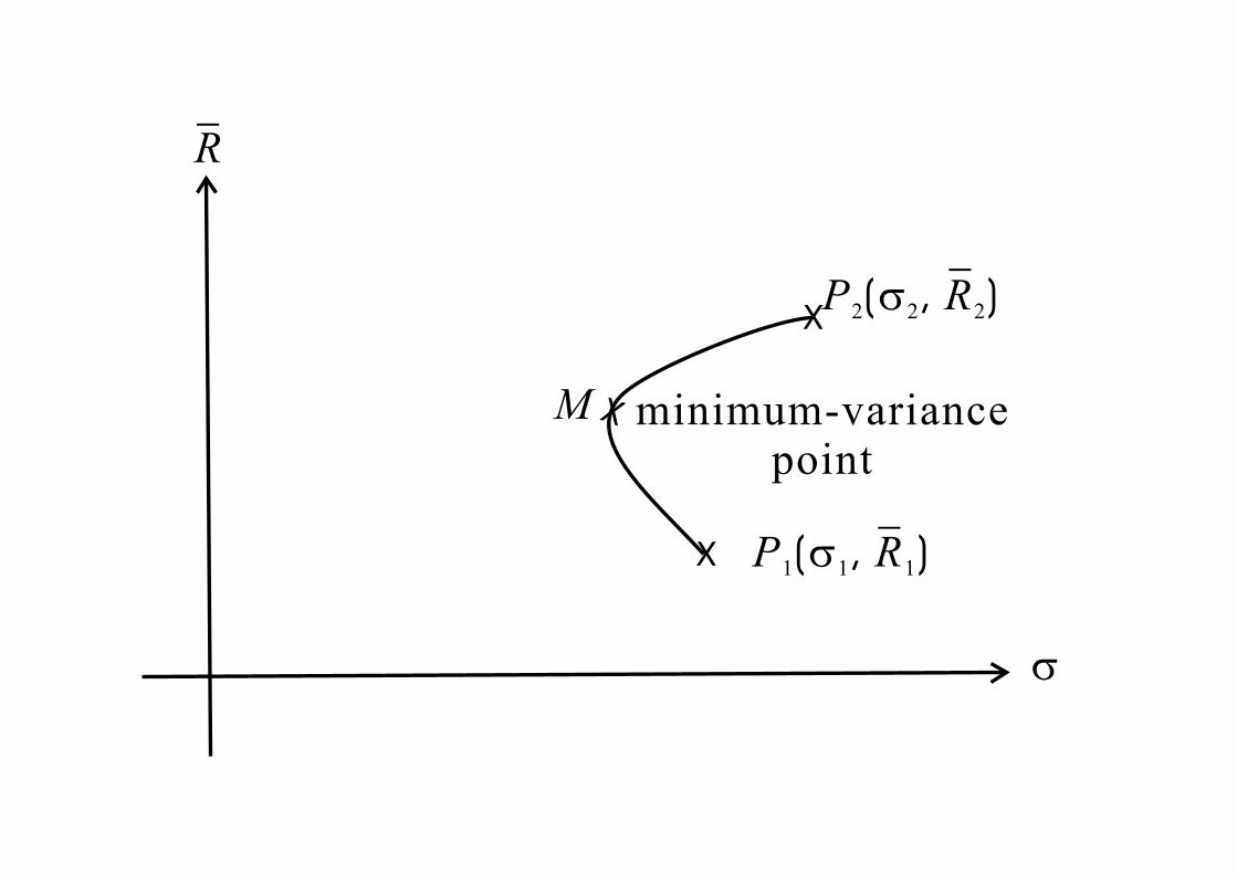
We represent the two assets in a mean-standard deviation diagram

(recall: standard deviation =√

variance)

As α varies, (σP , RP ) traces out a conic curve in the σ − R plane.

With ρ = −1, it is possible to have σ = 0 for some suitable choice

of weight.

In particular, when ρ = 1,

σP (α; ρ = 1) =√

(1− α)2σ21 + 2α(1− α)σ1σ2 + α2σ2

2

= (1− α)σ1 + ασ2.

This is the straight line joining P1(σ1, R1) and P2(σ2, R2).

When ρ = −1, we have

σP (α; ρ = −1) =√

[(1− α)σ1 − ασ2]2 = |(1− α)σ1 − ασ2|.

When α is small (close to zero), the corresponding point is close to

P1(σ1, R1). The line AP1 corresponds to

σP (α; ρ = −1) = (1− α)σ1 − ασ2.

The point A corresponds to α =σ1

σ1 + σ2.

The quantity (1 − α)σ1 − ασ2 remains positive until α =σ1

σ1 + σ2.

When α >σ1

σ1 + σ2, the locus traces out the upper line AP2.

Suppose −1 < ρ < 1, the minimum variance point on the curve that

represents various portfolio combinations is determined by

∂σ2P

∂α= −2(1− α)σ2

1 + 2ασ22 + 2(1− 2α)ρσ1σ2 = 0

↑set

giving

α =σ21 − ρσ1σ2

σ21 − 2ρσ1σ2 + σ2

2

.

Mathematical formulation of Markowitz’s mean-variance analysis

minimize1

2

N∑

i=1

N∑

j=1

wiwjσij

subject toN∑

i=1

wiRi = µP andN∑

i=1

wi = 1.

Solution

We form the Lagrangian

L =1

2

N∑

i=1

N∑

j=1

wiwjσij − λ1

(N∑

i=1

wi − 1

)− λ2

(N∑

i=1

wiRi − µP

)

where λ1 and λ2 are Lagrangian multipliers.

We then differentiate L with respect to wi and set the derivative to zero.

∂L

∂wi=

N∑

j=1

σijwj − λ1 − λ2Ri = 0, i = 1,2, · · · , N. (1)

∂L

∂λ1=

N∑

i=1

wi − 1 = 0; (2)

∂L

∂λ2=

N∑

i=1

wiRi − µP = 0. (3)

From Eq. (1), the portfolio weight admits solution of the form

w∗ = Ω−1(λ11+ λ2µ) (4)

where 1 = (1 1 · · ·1)T and µ = (R1 R2 · · ·RN)T .

To determine λ1 and λ2, we apply the two constraints

1 = 1TΩ−1Ωw∗ = λ11

TΩ−11+ λ21

TΩ−1µ. (5)

µP = µTΩ−1Ωw∗ = λ1µTΩ−11+ λ2µTΩ−1µ. (6)

Write a = 1TΩ−11, b = 1T

Ω−1µ and c = µTΩ−1µ, we have

1 = λ1a + λ2b and µP = λ1b + λ2c.

Solving for λ1 and λ2 : λ1 =c− bµP

∆and λ2 =

aµP − b

∆, where

∆ = ac− b2.

Note that λ1 and λ2 have dependence on µP , which is the target

mean prescribed in the variance minimization problem.

Assume µ 6= h1, and Ω−1 exists. Since Ω is positive definite, so

a > 0, c > 0. By virtue of the Cauchy-Schwarz inequality, ∆ > 0.

The minimum portfolio variance for a given value of µP is given by

σ2P = w∗TΩw∗ = w∗TΩ(λ1Ω

−11+ λ2Ω−1µ)

= λ1 + λ2µP =aµ2

P − 2bµP + c

∆.

The set of minimum variance portfolios is represented by a parabolic

curve in the σ2P − µP plane. The parabolic curve is generated by

varying the value of the parameter µP .

How about the asymptotic values of limµ→±∞

dµP

dσP?

dµP

dσP=

dµP

dσ2P

dσ2P

dσP

=∆

2aµP − 2b2σP

=

√∆

aµP − b

√aµ2

P − 2bµP + c

so that

limµ→±∞

dµP

dσP= ±

√∆

a.

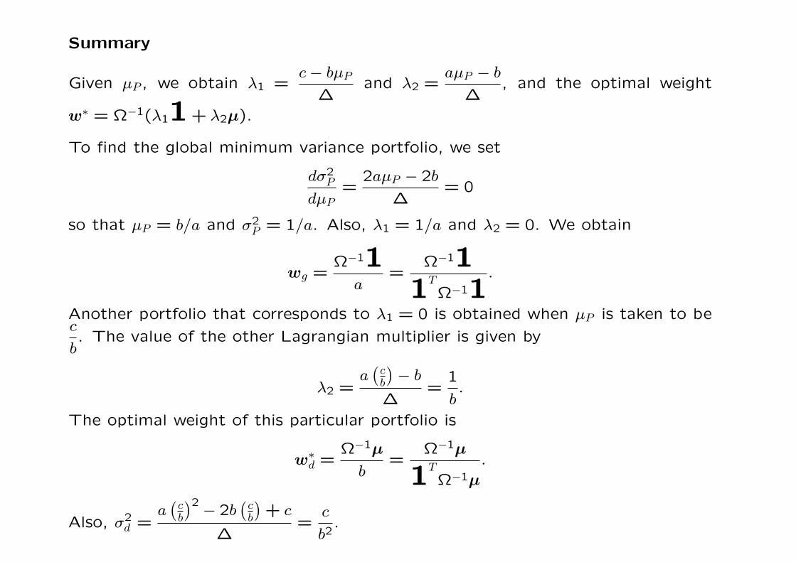
Summary

Given µP , we obtain λ1 =c− bµP

∆and λ2 =

aµP − b

∆, and the optimal weight

w∗ = Ω−1(λ11+ λ2µ).

To find the global minimum variance portfolio, we set

dσ2P

dµP=

2aµP − 2b

∆= 0

so that µP = b/a and σ2P = 1/a. Also, λ1 = 1/a and λ2 = 0. We obtain

wg =Ω−11

a=

Ω−111

T

Ω−11.

Another portfolio that corresponds to λ1 = 0 is obtained when µP is taken to bec

b. The value of the other Lagrangian multiplier is given by

λ2 =a

(cb

)− b

∆=

1

b.

The optimal weight of this particular portfolio is

w∗d =

Ω−1µ

b=

Ω−1µ

1T

Ω−1µ

.

Also, σ2d =

a(

cb

)2 − 2b(

cb

)+ c

∆=

c

b2.

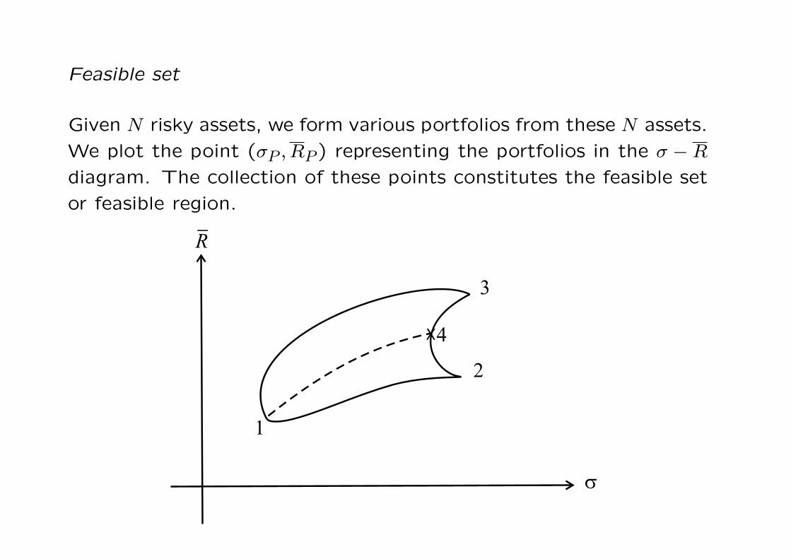
Feasible set

Given N risky assets, we form various portfolios from these N assets.

We plot the point (σP , RP ) representing the portfolios in the σ −R

diagram. The collection of these points constitutes the feasible set

or feasible region.

Consider a 3-asset portfolio, the various combinations of assets 2

and 3 sweep out a curve between them (the particular curve taken

depends on the correlation coefficient ρ12).

A combination of assets 2 and 3 (labelled 4) can be combined with

asset 1 to form a curve joining 1 and 4. As 4 moves between 2 and

3, the curve joining 1 and 4 traces out a solid region.

Properties of feasible regions

1. If there are at least 3 risky assets (not perfectly correlated

and with different means), then the feasible set is a solid two-

dimensional region.

2. The feasible region is convex to the left. That is, given any two

points in the region, the straight line connecting them does not

cross the left boundary of the feasible region.

The left boundary of a feasible region is called the minimum variance

set. The most left point on the minimum variance set is called the

minimum variance point. The portfolios in the minimum variance

set are called frontier funds.

For a given level of risk, only those portfolios on the upper half

of the efficient frontier are desired by investors. They are called

efficient funds.

A portfolio w∗ is said to be mean-variance efficient if there exists

no portfolio w with µP ≥ µ∗P and σ2P ≤ σ∗2P . That is, you cannot find

a portfolio that has a higher return and lower risk than those for an

efficient portfolio.

Two-fund theorem

Two frontier funds (portfolios) can be established so that any fron-

tier portfolio can be duplicated, in terms of mean and variance, as

a combination of these two. In other words, all investors seeking

frontier portfolios need only invest in combinations of these two

funds.

Remark

Any convex combination (that is, weights are non-negative) of ef-

ficient portfolios is an efficient portfolio. Let αi ≥ 0 be the weight

of Fund i whose rate of return is Rif . Since E

[RI

f

]≥ b

afor all i, we

haven∑

i=1

αiE[Ri

f

]≥

n∑

i=1

αib

a=

b

a.

Proof

Let w1 = (w11 · · ·w1

n), λ11, λ1

2 and w2 = (w21 · · ·w2

n)T , λ2, µ2 are two

known solutions to the minimum variance formulation with expected

rates of return µ1P and µ2

P , respectively.

n∑

j=1

σijwj − λ1 − λ2Ri = 0, i = 1,2, · · · , n (1)

n∑

i=1

wiri = µP (2)

n∑

i=1

wi = 1. (3)

It suffices to show that αw1 + (1 − α)w2 is a solution corresponds

to the expected rate of return αµ1P + (1− α)µ2

P .

1. αw1 +(1−α)w2 is a legitimate portfolio with weights that sum

to one.

2. Eq. (1) is satisfied by αw1 + (1 − α)w2 since the system of

equations is linear.

3. Note thatn∑

i=1

[αw1

i + (1− α)w2i

]Ri

= αn∑

i=1

w1i Ri + (1− α)

n∑

i=1

w2i Ri

= αµ1P + (1− α)µ2

P .

Proposition

Any minimum variance portfolio with target mean µP can be uniquely

decomposed into the sum of two portfolios

w∗P = Awg + (1−A)wd

where A = λ1a =c− bµP

∆a.

Proof

For a minimum-variance portfolio whose solution of the Lagrangian

multipliers are λ1 and λ2, the optimal weight is

w∗P = λ1(Ω

−11+ Ω−1µ) = λ1(awg) + λ2(bwd).

Observe that the sum of weights is

λ1a + λ2b = ac− µP b

∆+ b

µPa− b

∆=

ac− b2

∆= 1.

We set λ1a = A and λ2b = 1−A.

Indeed, any two minimum-variance portfolios can be used to substi-

tute for wg and wd. Suppose

wu = (1− u)wg + uwd

wv = (1− v)wg + vwd

we then solve for wg and wd in terms of wu and wv. Then

w∗P = λ1awg + (1− λ1a)wd

=λ1a + v − 1

v − uwu +

1− u− λ1a

v − uwv,

where sum of coefficients = 1.

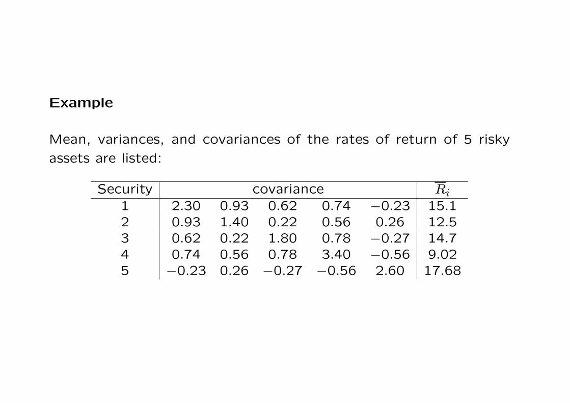
Example

Mean, variances, and covariances of the rates of return of 5 risky

assets are listed:

Security covariance Ri1 2.30 0.93 0.62 0.74 −0.23 15.12 0.93 1.40 0.22 0.56 0.26 12.53 0.62 0.22 1.80 0.78 −0.27 14.74 0.74 0.56 0.78 3.40 −0.56 9.025 −0.23 0.26 −0.27 −0.56 2.60 17.68

Solution procedure to find the two funds in the minimum variance

set:

1. Set λ1 = 1 and λ2 = 0; solve the system of equations

5∑

j=1

σijv1j = 1, i = 1,2, · · · ,5.

Normalize v1k ’s so that they sum to one

w1i =

v1i∑n

j=1 v1j

.

After normalization, this gives the solution to wg, where λ1 =1

aand λ2 = 0.

2. Set λ1 = 0 and λ2 = 1; solve the system of equations:

5∑

j=1

σijv2j = Ri, i = 1,2, · · · ,5.

Normalize v2i ’s to obtain w2

i .

After normalization, this gives the solution to wd, where λ1 = 0

and λ2 =1

b.

The above procedure avoids the computation of a = 1TΩ−11

and b = 1TΩ−1µ.

security v1 v2 w1 w2

1 0.141 3.652 0.088 0.1582 0.401 3.583 0.251 0.1553 0.452 7.284 0.282 0.3144 0.166 0.874 0.104 0.0385 0.440 7.706 0.275 0.334

mean 14.413 15.202variance 0.625 0.659

standard deviation 0.791 0.812

* Note that w1 corresponds to the global minimum variance point.

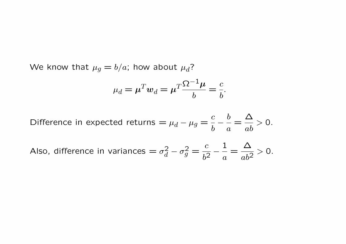
We know that µg = b/a; how about µd?

µd = µTwd = µT Ω−1µ

b=

c

b.

Difference in expected returns = µd − µg =c

b− b

a=

∆

ab> 0.

Also, difference in variances = σ2d − σ2

g =c

b2− 1

a=

∆

ab2> 0.

How about the covariance of portfolio returns for any two minimum

variance portfolios?

Write

RuP = wT

uR and RvP = wT

v R

where R = (R1 · · ·RN)T . Recall that

σgd = cov

Ω−11

aR,

Ω−1µ

bR

=

Ω−11

a

T

Ω

(Ω−1µ

b

)

=1Ω−1µ

ab=

1

asince b = 1Ω−1µ.

cov(RuP , Rv

P ) = (1− u)(1− v)σ2g + uvσ2

d + [u(1− v) + v(1− u)]σgd

=(1− u)(1− v)

a+

uvc

b2+

u + v − 2uv

a

=1

a+

uv∆

ab2.

In particular,

cov(Rg, RP ) = wTg ΩwP =

1Ω−1ΩwP

a=

1

a= var(Rg)

for any portfolio wP .

For any Portfolio u, we can find another Portfolio v such that these

two portfolios are uncorrelated. This can be done by setting

1

a+

uv∆

ab2= 0.

Inclusion of a riskfree asset

Consider a portfolio with weight α for a risk free asset and 1−α for

a risky asset. The mean of the portfolio is

RP = αRf + (1− α)Rj (note that Rf = Rf).

The covariance σfj between the risk free asset and any risky asset

is zero since

E[(Rj −Rj) (Rf −Rf)︸ ︷︷ ︸zero

= 0.

Therefore, the variance of portfolio σ2P is

σ2P = α2 σ2

f︸︷︷︸zero

+(1− α)2σ2j + 2α(1− α) σfj︸︷︷︸

zero

so that σP = |1− α|σj.

The points representing (σP , RP ) for varying values of α lie on a

straight line joining (0, Rf) and (σj, Rj).

If borrowing of risk free asset is allowed, then α can be negative. In

this case, the line extends beyond the right side of (σj, Rj) (possibly

up to infinity).

Consider a portfolio with N risky assets originally, what is the impact

of the inclusion of a risk free asset on the feasible region?

Lending and borrowing of risk free asset is allowed

For each original portfolio formed using the N risky assets, the new

combinations with the inclusion of the risk free asset trace out the

infinite straight line originating from the risk free point and passing

through the point representing the original portfolio.

The totality of these lines forms an infinite triangular feasible region

bounded by the two tangent lines through the risk free point to the

original feasible region.

No shorting of risk free asset

The line originating from the risk free point cannot be extended

beyond points in the original feasible region (otherwise entail bor-

rowing of the risk free asset). The new feasible region has straight

line front edges.

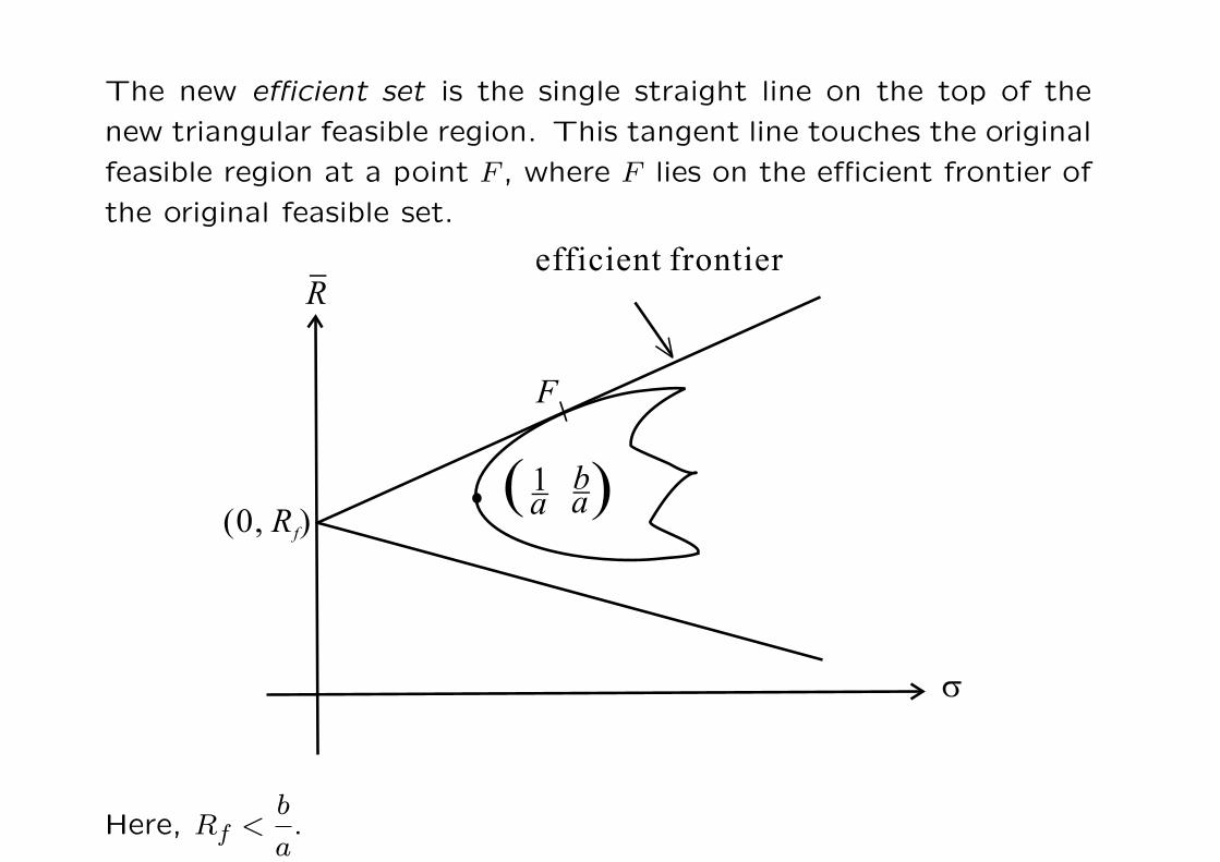
The new efficient set is the single straight line on the top of the

new triangular feasible region. This tangent line touches the original

feasible region at a point F , where F lies on the efficient frontier of

the original feasible set.

Here, Rf <b

a.

One fund theorem

Any efficient portfolio (any point on the upper tangent line) can be

expressed as a combination of the risk free asset and the portfolio

(or fund) represented by F .

“There is a single fund F of risky assets such that any efficient

portfolio can be constructed as a combination of the fund F and

the risk free asset.”

Remark Under the assumptions that

• every investor is a mean-variance optimizer

• they all agree on the probabilistic structure of assets

• unique risk free asset

Then everyone will purchase a single fund, market portfolio.

New Lagrangian formulation

minimizeσ2

P

2=

1

2wTΩw

subject to wTµ + (1−wT1)r = µP .

Define L =1

2wTΩw + λ[µP − r − (µ− r1)Tw]

∂L

∂wi=

N∑

j=1

σijwj − λ(µ− r1) = 0, i = 1,2, · · · , N (1)

∂L

∂λ= 0 giving (µ− r1)Tw = µP − r. (2)

Solving (1): w∗ = λΩ−1(µ− r1). Substituting into (2)

µP − r = λ(µ− r1)TΩ−1(µ− r1) = λ(c− 2rb + r2a).

Lastly, the relation between µP and σP is given by the following pair

of half lines

σ2P = w∗TΩw∗ = λ(w∗T µ− rw∗T1)

= λ(µP − r) = (µP − r)2/(c− 2rb + r2a).

With the inclusion of the riskfree asset, the set of minimum variance

portfolios are represented by portfolios on the two half lines

Lup : µP − r = σP

√ar2 − 2br + c (1a)

Llow : µP − r = −σP

√ar2 − 2br + c. (1b)

Recall that ar2−2br+ c > 0 for all values of r since ∆ = ac− b2 > 0.

The minimum variance portfolios without the riskfree asset lie on

the hyperbola

σ2P =

aµ2P − 2bµP + c

∆.

When r < µg =b

a, the upper half line is a tangent to the hyperbola.

The tangency portfolio is the tangent point to the efficient frontier

(upper part of the hyperbolic curve) through the point (0, r).

The tangency portfolio M is represented by the point (σP,M , µMP ),

and the solution to σP,M and µMP are obtained by solving simultane-

ously

σ2P =

aµ2P − 2bµP + c

∆

µP = r + σP

√c− 2rb + r2a.

Once µP is obtained, we solve for λ and w∗ from

λ =µP − r

c− 2rb + r2aand w∗ = λΩ−1(µ− r1).

The tangency portfolio M is shown to be

w∗M =

Ω−1(µ− r1)

b− ar, µM

P =c− br

b− arand σ2

P,M =c− 2rb + r2a

(b− ar)2.

When r <b

a, it can be shown that µM

P > r. Note that

(µM

P − b

a

) (b

a− r

)=

(c− br

b− ar− b

a

)b− ar

a

=c− br

a− b2

a2+

br

a

=ca− b2

a2=

∆

a2> 0,

so we deduce that µMP >

b

a> r, where µg =

b

a. Indeed, we can

deduce (σP,M , µMP ) does not lie on the upper half line if r ≥ b

a.

When r <b

a, we have the following properties on the minimum

variance portfolios.

1. Efficient portfolios

Any portfolio on the upper half line

µP = r + σP

√ar2 − 2br + c

within the segment FM joining the two points (0, r) and M

involves long holding of the market portfolio and riskfree asset,

while those outside FM involves short selling of the riskfree asset

and long holding of the market portfolio.

2. Any portfolio on the lower half line

µP = r − σP

√ar2 − 2br + c

involves short selling of the market portfolio and investing the

proceeds in the riskfree asset. This represents non-optimal in-

vestment strategy since the investor faces risk but gains no extra

expected return above r.

What happens when r = b/a? The half lines become

µP = r ± σP

√c− 2

(b

a

)b± b2

a= r ± σP

√∆

a,

which correspond to the asymptotes of the feasible region with risky

assets only.

When r =b

a, µM

P does not exist. Recall that

w∗ = λΩ−1(µ− r1) so that

1Tw = λ(1Ω−1µ− r1Ω−11) = λ(b− ra).

When r = b/a,1Tw = 0 as λ is finite. Any minimum variance port-

folio involves investing everything in the riskfree asset and holding

a portfolio of risky assets whose weights sum to zero.

When r >b

a, only the lower half line touches the feasible region with

risky assets only.

Any portfolio on the upper half line involves short selling of the

tangency portfolio and investing the proceeds in the riskfree asset.

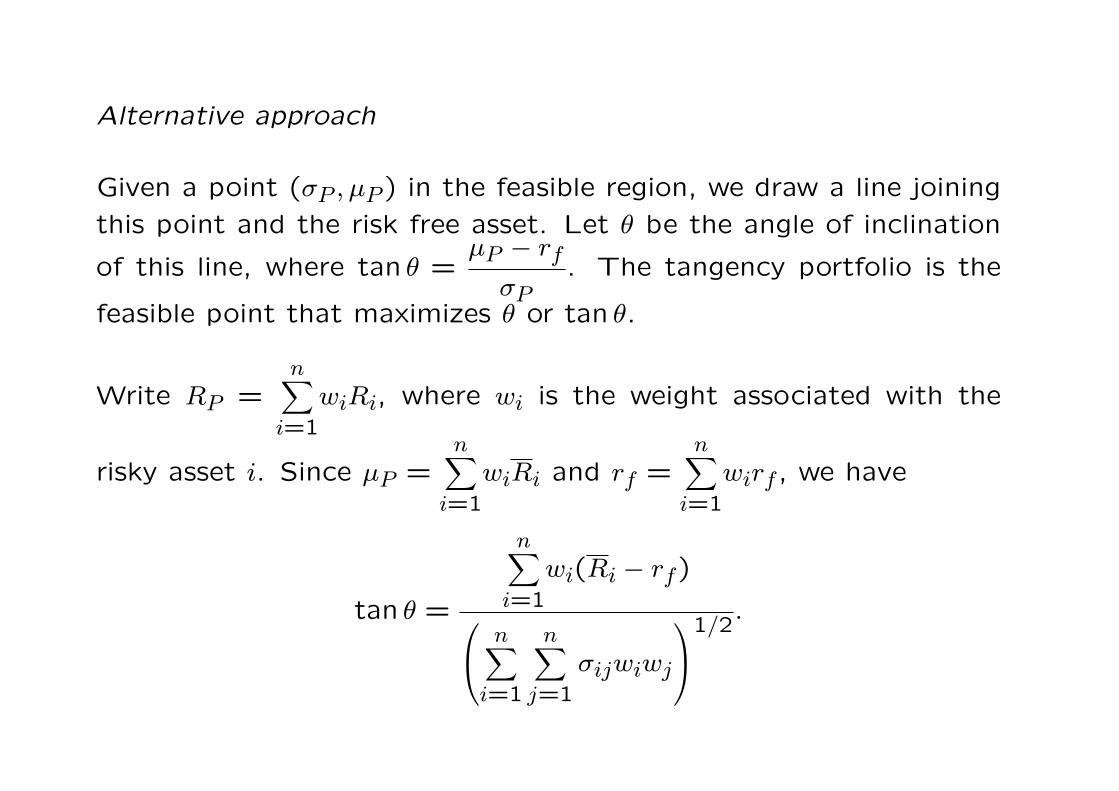
Alternative approach

Given a point (σP , µP ) in the feasible region, we draw a line joining

this point and the risk free asset. Let θ be the angle of inclination

of this line, where tan θ =µP − rf

σP. The tangency portfolio is the

feasible point that maximizes θ or tan θ.

Write RP =n∑

i=1

wiRi, where wi is the weight associated with the

risky asset i. Since µP =n∑

i=1

wiRi and rf =n∑

i=1

wirf , we have

tan θ =

n∑

i=1

wi(Ri − rf)

n∑

i=1

n∑

j=1

σijwiwj

1/2.

Set the derivative of tan θ with respect to each wk equal to zero:-

∂

∂witan θ

=

(Ri − rf

)

n∑

i,j=1

σijwiwj

1/2

−[

n∑

i=1

wi(Ri − rf)

]

n∑

i,j=1

σi,jwiwj

−1/2

n∑

j=1

σijwj

n∑

i,j=1

σijwiwj

= 0.

This leads to the following system of equations:-

n∑

j=1

σijwj = λ(Ri − rf), λ is some constant, i = 1,2, · · · , n.

Hint Use the following relation

∂

∂wi

∑

i,j

wiσijwj

1/2

=

∑

i,j

wiσijwj

−1/2 n∑

j=1

σijwj.

We write λvj = wj for each j, the above system becomes

n∑

j=1

σijvj = ri − rf , i = 1,2, · · · , n.

We then solve for vj by a linear system solver.

Finally, we normalize wj’s by wj =vj∑n

j=1 vk, j = 1, · · · , n.

Example (5 risky assets and one risk free asset)

Data of the 5 risky assets are given in the earlier example, and

rf = 10%.

The system of linear equations to be solved is

5∑

j=1

σijvj = Ri − rf = 1×Ri − rf × 1, i = 1,2, · · · ,5.

Recall that v1 and v2 in the earlier example are solutions to

5∑

j=1

σijv1j = 1 and

5∑

j=1

σijv2j = Ri, respectively.

Hence, vj = v2j − rfv1

j , j = 1,2, · · · ,5 (numerically, we take rf =

10%).

Addition of risk tolerance factor

Maximize 2τµP − σ2P , with τ ≥ 0, where τ is the risk tolerance.

Optimization problem: maxw∈RN

2τµP − σ2P subject to 1 ·w = 1.

Remark

τ is closely related to the relative risk aversion coefficient. Given an

initial wealth W0 and under a portfolio choice w, the end-of-period

wealth is W0(1 + RP ). Let µP = E[RP ] and σ2P = var(RP ).

Consider the Taylor expansion

u[W0(1 + RP )] ≈ u(W0) + W0u′(W0)RP +W2

0

2u′′(W0)R

2P + · · · .

Neglecting third and higher order moments and noting E[R2P ] =

σ2P + µ2

P .

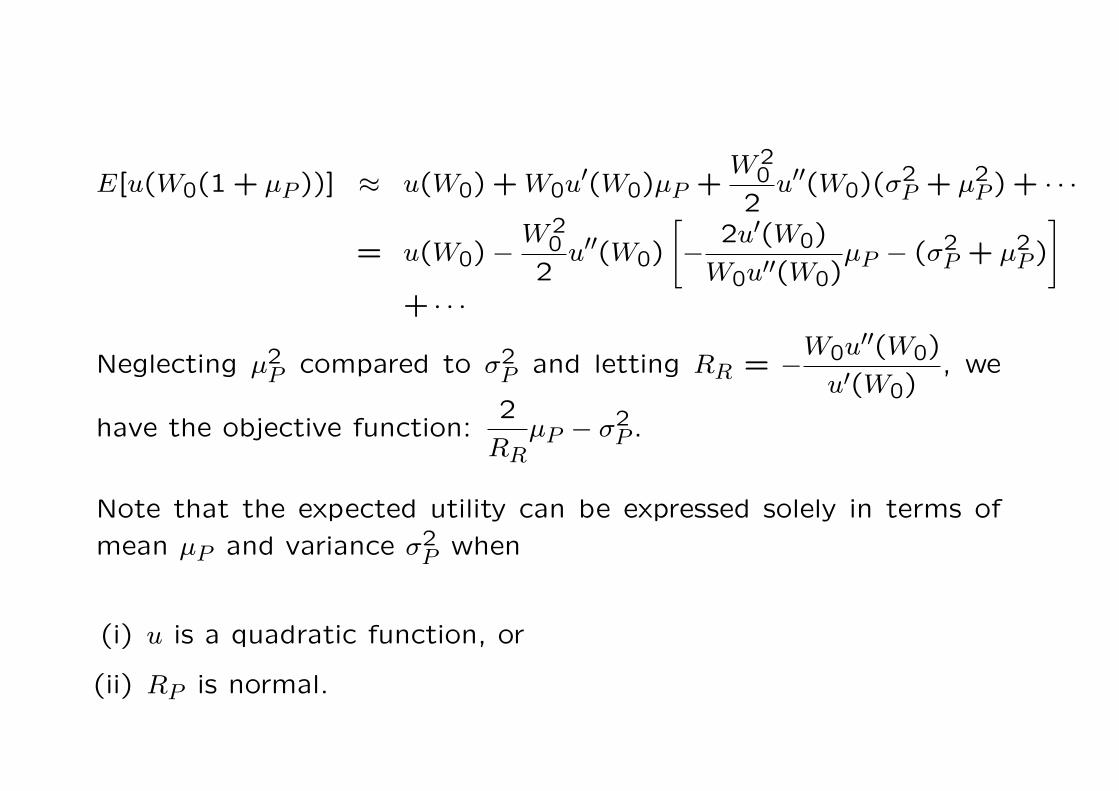
E[u(W0(1 + µP ))] ≈ u(W0) + W0u′(W0)µP +W2

0

2u′′(W0)(σ

2P + µ2

P ) + · · ·

= u(W0)−W2

0

2u′′(W0)

[− 2u′(W0)

W0u′′(W0)µP − (σ2

P + µ2P )

]

+ · · ·

Neglecting µ2P compared to σ2

P and letting RR = −W0u′′(W0)

u′(W0), we

have the objective function:2

RRµP − σ2

P .

Note that the expected utility can be expressed solely in terms of

mean µP and variance σ2P when

(i) u is a quadratic function, or

(ii) RP is normal.

Quadratic optimization problem

maxw∈RN

[2τµTw −wTΩw] subject to 1 ·w = 1.

The Lagrangian formulation becomes:

L(w;λ) = 2τµTw −wTΩw + λ(wT1− 1).

The first order conditions are

2τµ− 2Ωw∗ + λ1 = 0

1 ·w∗ = 1.

Express the optimal solution w∗ as wg + τz∗, τ ≥ 0.

1. When τ = 0,2Ωw = λ01 and 1Twg = 1

wg =λ0

2Ω−11 and 1 = 1T

wg =λ0

21T

Ω−11

hence

wg =Ω−11

1TΩ−11

(independent of µ).

2. When τ ≥ 0, w = τΩ−1µ +λ

2Ω−11.

1 = 1Tw = τ1T

Ω−1µ +λ

21T

Ω−11 so thatλ

2=

1− τ1Ω−1µ

1TΩ−11

.

w = τΩ−1µ+1− τ1T

Ω−1µ

1TΩ−11

Ω−11 = τ

Ω−1µ− 1T

Ω−1µ

1TΩ−11

Ω−11+wg.

We obtain

z∗ = Ω−1µ− 1TΩ−1µ

1TΩ−11

Ω−11 and 1Tz∗ = 0.

Observe that cov(Rwg, Rz∗) = z∗TΩwg = 0.

Financial interpretation

wg leads to a minimum risk position. This position is modified

by investing in the self-financing portfolio z∗ so as to maximize

2τµTw −wTΩ−1w.

Efficient frontier

Consider

µP = µT (wg + τz∗) = µg + τµP,z∗

σ2P = σ2

g + 2τ cov(Rwg, Rz∗)︸ ︷︷ ︸z∗T Ωwg=0

+ τ2σ2z∗.

By eliminating τ, σ2P = σ2

g +

(µP − µg

µP,z∗

)2

σ2z∗. Hence, the frontier is

parabolic in the (µP , σ2P )-diagram and hyperbolic in the (µP , σP )-

diagram.

Inclusion of riskfree asset (deterministic rate of return R0 = r)

Let w = (w0 · · ·wN)T andN∑

i=0

wi = 1.

Lagrangian formulation becomes

L = 2τ µT w − wTΩw + λ(wT1− 1) + 2τw0r + λw0

where w = (w1 · · ·wn)T ∈ RN , µ = (µ1 · · ·µN)T ∈ RN ,1T= (1 · · ·1)T ∈

RN .

The optimality conditions become

2τr + λ = 0 (i)

2τ µ− 2Ωw∗ + λ1 = 0 (ii)N∑

i=0

w∗i = 1 (iii)

Estimation of risk tolerance (inverse problem)

Reverse optimization: given an efficient portfolio w∗, it is possible

to express τ in terms of var(R∗P ) and µ∗P . Taking the inner product

of w∗ with (ii), we obtain

2τ(rw∗0 + µT w∗)− 2w∗TΩw + λ = 0.

By eliminating λ using (i), we obtain the implied risk tolerance as

follows:

τ =var(R∗P )

µ∗P − r.

Marginal utilities

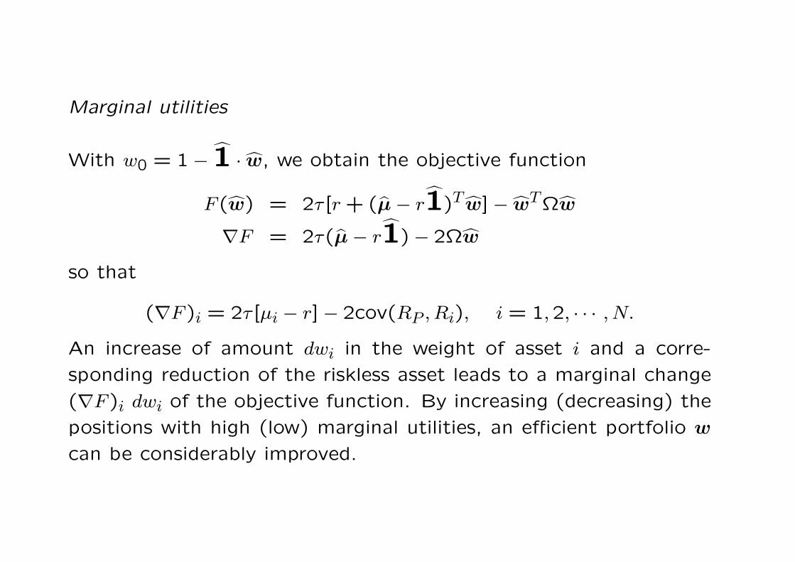
With w0 = 1− 1 · w, we obtain the objective function

F (w) = 2τ [r + (µ− r1)T w]− wTΩw

∇F = 2τ(µ− r1)− 2Ωw

so that

(∇F )i = 2τ [µi − r]− 2cov(RP , Ri), i = 1,2, · · · , N.

An increase of amount dwi in the weight of asset i and a corre-

sponding reduction of the riskless asset leads to a marginal change

(∇F )i dwi of the objective function. By increasing (decreasing) the

positions with high (low) marginal utilities, an efficient portfolio w

can be considerably improved.

Summary

1. The objective function 2τµTw −wTΩw represents a balance of

maximizing return 2τµTw against risk wTΩw, where the weigh-

ing factor τ is related to the reciprocal of relative risk aversion

coefficient RR.

2. The optimal solution takes the form

w∗ = wg + τz∗

where wg is the portfolio weight of the global minimum variance

portfolio and the weights in z∗ are summed to zero.

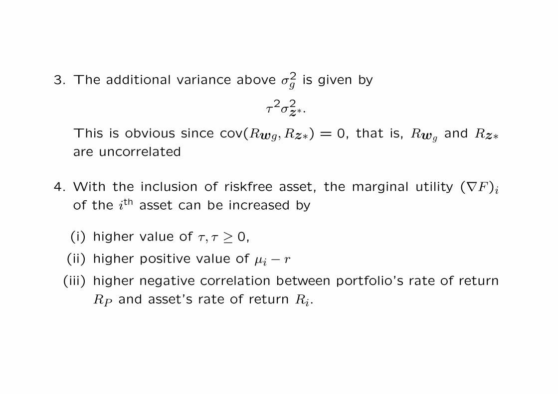
3. The additional variance above σ2g is given by

τ2σ2z∗.

This is obvious since cov(Rwg, Rz∗) = 0, that is, Rwg and Rz∗are uncorrelated

4. With the inclusion of riskfree asset, the marginal utility (∇F )i

of the ith asset can be increased by

(i) higher value of τ, τ ≥ 0,

(ii) higher positive value of µi − r

(iii) higher negative correlation between portfolio’s rate of return

RP and asset’s rate of return Ri.

Asset-Liability Model

Liabilities of a pension fund = future benefits − future contributions

Market value can hardly be determined since liabilities are not readily

marketable. Assume that some specific accounting rules are used to

calculate an initial value L0. If the same rule is applied one period

later, a value L1 results.

Growth rate of the liabilities = RL =L1 − L0

L0, where RL is expected

to depend on the changes of interest rate structure, mortality and

other stochastic factors. Let A0 be the initial value of assets. The

investment strategy of the pension fund is given by the portfolio

choice w.

Surplus optimization

Depending on the portfolio choice w, the surplus gain after one

period

S1 − S0 = A0Rw − L0RL, where S0 = A0 − L0.

The return on surplus is defined by

RS =S1 − S0

A0= Rw − 1

f0RL

where f0 = A0/L0 is the initial funding ratio.

Maximization formulation:-

maxw∈RN

2τE

[Rw − 1

f0RL

]− var

(Rw − 1

f0RL

)

subject toN∑

i=1

wi = 1. Note that1

f0RL and var(RL) are independent

of w so that they do not enter into the objective function.

maxw∈RN

2τE[Rw]− var(Rw) +

2

f0cov(Rw, RL)

subject toN∑

i=1

wi = 1. Recall that

cov(Rw, RL) = cov

N∑

i=1

wiRi, RL

=

N∑

i=1

wicov(Ri, RL).

maxw∈RN

2τµTw + 2γTw −wTΩw subject to 1Tw = 1,

where γT = (γ1 · · · γN) with γi =1

f0cov(Ri, RL),

µT = (µ1 · · ·µN) with µi = E[Ri], σij = cov(Ri, Rj).

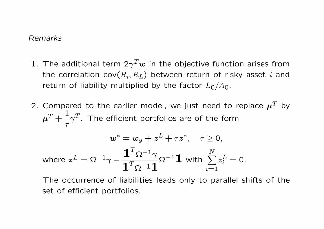
Remarks

1. The additional term 2γTw in the objective function arises from

the correlation cov(Ri, RL) between return of risky asset i and

return of liability multiplied by the factor L0/A0.

2. Compared to the earlier model, we just need to replace µT by

µT +1

τγT . The efficient portfolios are of the form

w∗ = wg + zL + τz∗, τ ≥ 0,

where zL = Ω−1γ − 1TΩ−1γ

1TΩ−11

Ω−11 withN∑

i=1

zLi = 0.

The occurrence of liabilities leads only to parallel shifts of the

set of efficient portfolios.

The mean-variance criterion can be reconciled with the expected

utility approach in either of two ways: (1) using a quadratic utility

function, or (2) making the assumption that the random returns are

normal variables.

Quadratic utility

The quadratic utility function can be defined as U(x) = ax − b

2x2,

where a > 0 and b > 0. This utility function is really meaningful

only in the range x ≤ a/b, for it is in this range that the function is

increasing. Note also that for b > 0 the function is strictly concave

everywhere and thus exhibits risk aversion.

mean-variance analysis ⇔ maximum expected utility criterion

based on quadratic utility

Suppose that a portfolio has a random wealth value of y. Using the

expected utility criterion, we evaluate the portfolio using

E[U(y)] = E

[ay − b

2y2

]

= aE[y]− b

2E[y2]

= aE[y]− b

2(E[y])2 − b

2var(y).

The optimal portfolio is the one that maximizes this value with

respect to all feasible choices of the random wealth variable y.

Normal Returns

When all returns are normal random variables, the mean-variance

criterion is also equivalent to the expected utility approach for any

risk-averse utility function.

To deduce this, select a utility function U . Consider a random

wealth variable y that is a normal random variable with mean value

M and standard deviation σ. Since the probability distribution is

completely defined by M and σ, it follows that the expected utility

is a function of M and σ. If U is risk averse, then

E[U(y)] = f(M, σ), with∂f

∂M> 0 and

∂f

∂σ< 0.

• Now suppose that the returns of all assets are normal random

variables. Then any linear combination of these asset is a normal

random variable. Hence any portfolio problem is therefore equiv-

alent to the selection of combination of assets that maximizes

the function f(M, σ) with respect to all feasible combinations.

• For a risky-averse utility, this again implies that the variance

should be minimized for any given value of the mean. In other

words, the solution must be mean-variance efficient.

• Portfolio problem is to find w∗ such that f(M, σ) is maximized

with respect to all feasible combinations.

Two fund monetary separation

Consider a financial market with the riskfree asset and several risky

assets, suppose the utility function satisfies

−u′(z)u′′(z)

= a + bz, valid for all z,

then the optimal portfolio at different wealth levels is given by the

combination of the riskfree asset and market fund consisting of the

risky assets. The relative proportions of risky assets in the market

fund remain the same, irrespective of W0.

Remark

The class of utility functions include

(i) quadratic utility(ii) log utility: a = 0(iii) exponential utility: b = 0(iv) power utility: a = 0.

Let W0 be the initial wealth, then the wealth amount a∗j(W0) of

risky asset j in the optimal portfolio satisfies

a∗j(W0) = αjh(W0) j = 1,2, · · · , n, and αj is independent of W0,

so that the relative proportion bj is given by

bj =a∗j(W0)

n∑

k=1

a∗k(W0)

=αj

n∑

k=1

αk

, independent of W0.

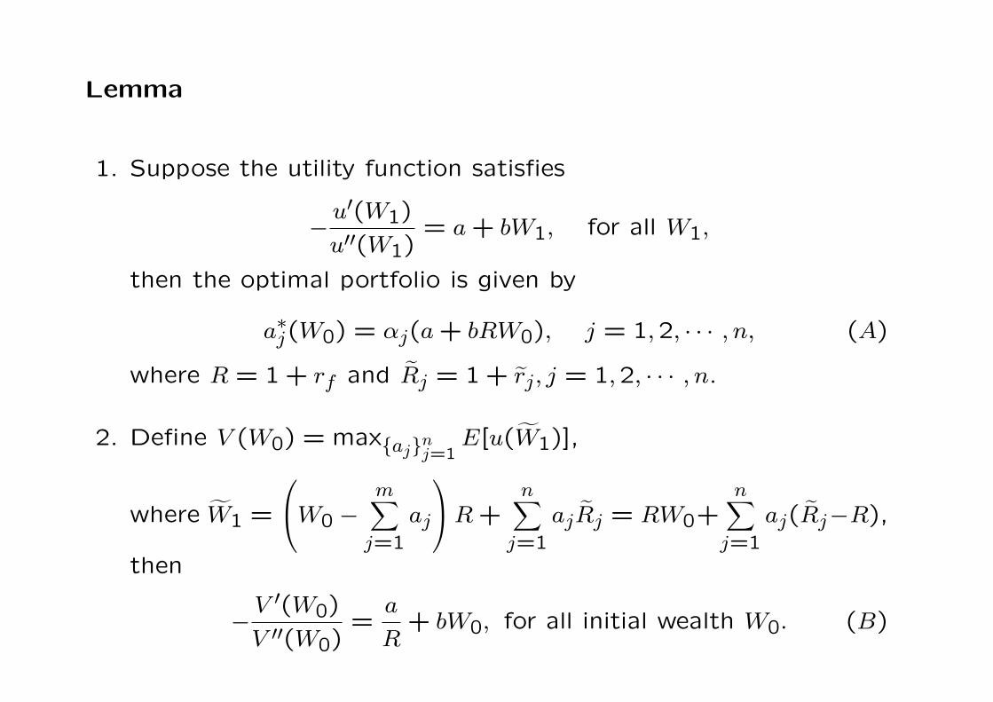
Lemma

1. Suppose the utility function satisfies

−u′(W1)

u′′(W1)= a + bW1, for all W1,

then the optimal portfolio is given by

a∗j(W0) = αj(a + bRW0), j = 1,2, · · · , n, (A)

where R = 1 + rf and Rj = 1 + rj, j = 1,2, · · · , n.

2. Define V (W0) = maxajnj=1E[u(W1)],

where W1 =

W0 −

m∑

j=1

aj

R +

n∑

j=1

ajRj = RW0+n∑

j=1

aj(Rj−R),

then

−V ′(W0)

V ′′(W0)=

a

R+ bW0, for all initial wealth W0. (B)

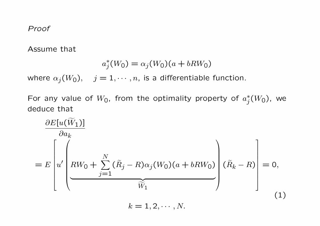
Proof

Assume that

a∗j(W0) = αj(W0)(a + bRW0)

where αj(W0), j = 1, · · · , n, is a differentiable function.

For any value of W0, from the optimality property of a∗j(W0), we

deduce that

∂E[u(W1)]

∂ak

= E

u′

RW0 +N∑

j=1

(Rj −R)αj(W0)(a + bRW0)

︸ ︷︷ ︸W1

(Rk −R)

= 0,

(1)

k = 1,2, · · · , N.

Next, we differentiate eq (1) with respect to W0. First, we observe

that

dW1

dW0= R

1 +

N∑

j=1

(Rj −R)αj(W0)b

+N∑

j=1

dαj(W0)

dW0(Rj −R)(a + bRW0).

Hence, for the kth component, we obtain

N∑

j=1

E[u′′(W1)(Rj −R)(Rk −R)(a + bRW0)]dαj(W0)

dW0

= −E

u′′(W1)(Rk −R)R

1 +

N∑

j=1

(Rj −R)αj(W0)b

,

k = 1,2, · · · , N.

In matrix form, we have

E

(R1 −R)2 · · · (R1 −R)(RN −R)(R2 −R)(R1 −R) · · · (R2 −R)(RN −R)

... . . . ...(RN −R)(R1 −R) · · · (RN −R)2

u′′(W1)(a + bRW0)

dα1(W0)dW0

dα2(W0)dW0...

dαN(W0)dW0

= −

E

u′′(W1)(R1 −R)R[1 +

∑Nj=1(Rj −R)αj(W0)b

]

E

u′′(W1)(R2 −R)R[1 +

∑Nj=1(Rj −R)αj(W0)b

]

...

E

u′′(W1)(RN −R)R[1 +

∑Nj=1(Rj −R)αj(W0)b

]

(2)

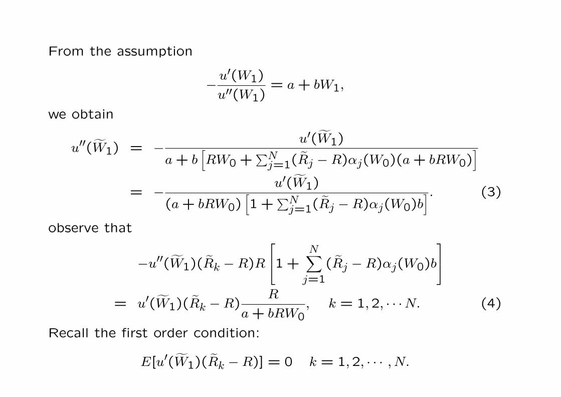
From the assumption

−u′(W1)

u′′(W1)= a + bW1,

we obtain

u′′(W1) = − u′(W1)

a + b[RW0 +

∑Nj=1(Rj −R)αj(W0)(a + bRW0)

]

= − u′(W1)

(a + bRW0)[1 +

∑Nj=1(Rj −R)αj(W0)b

]. (3)

observe that

−u′′(W1)(Rk −R)R

1 +

N∑

j=1

(Rj −R)αj(W0)b

= u′(W1)(Rk −R)R

a + bRW0, k = 1,2, · · ·N. (4)

Recall the first order condition:

E[u′(W1)(Rk −R)] = 0 k = 1,2, · · · , N.

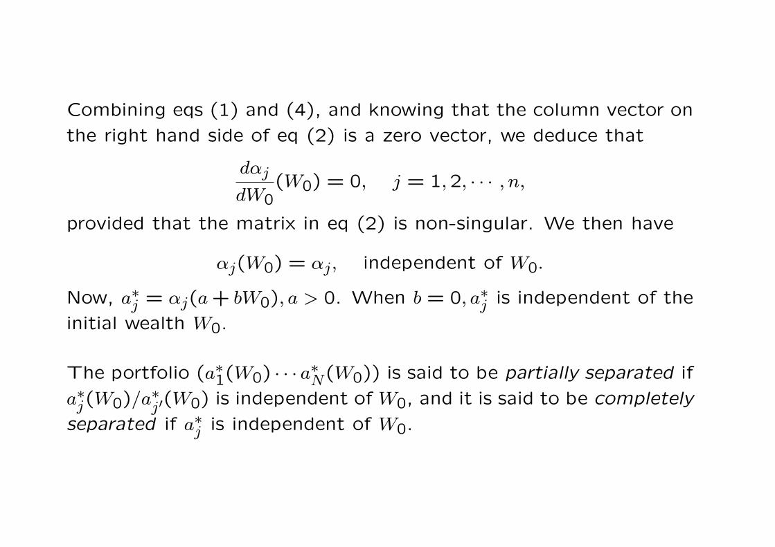
Combining eqs (1) and (4), and knowing that the column vector on

the right hand side of eq (2) is a zero vector, we deduce that

dαj

dW0(W0) = 0, j = 1,2, · · · , n,

provided that the matrix in eq (2) is non-singular. We then have

αj(W0) = αj, independent of W0.

Now, a∗j = αj(a + bW0), a > 0. When b = 0, a∗j is independent of the

initial wealth W0.

The portfolio (a∗1(W0) · · · a∗N(W0)) is said to be partially separated if

a∗j(W0)/a∗j′(W0) is independent of W0, and it is said to be completely

separated if a∗j is independent of W0.

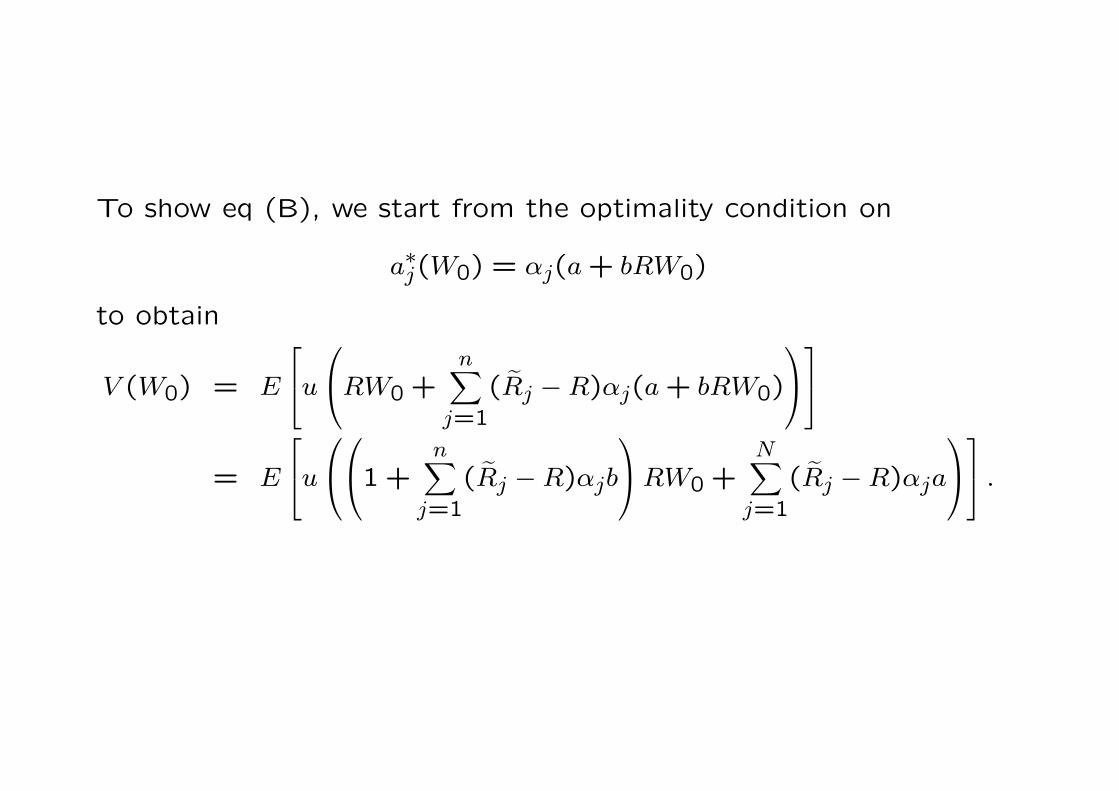
To show eq (B), we start from the optimality condition on

a∗j(W0) = αj(a + bRW0)

to obtain

V (W0) = E

u

RW0 +

n∑

j=1

(Rj −R)αj(a + bRW0)

= E

u

1 +

n∑

j=1

(Rj −R)αjb

RW0 +

N∑

j=1

(Rj −R)αja

.

Differentiate V (W0) twice with respect to W0

V ′(W0) = E

u′(W1)R

1 +

n∑

j=1

(Rj −R)αjb

V ′′(W0) = E

u′′(W1)R

2

1 +

n∑

j=1

(Rj −R)αjb

2 .

Relating u′′(W1) with u′(W1) using eq (3), we obtain

V ′′(W0) = −RE

[u′(W1)R

(1 +

∑nj=1(Rj −R)αjb

)]

a + bRW0= − R

a + bRW0V ′(W0).

Combining the results

−V ′(W0)

V ′′(W0)=

a

R+ bW0.

Formulation for finding the optimal portfolio

Let α be the weight of the riskfree asset so that the wealth invested in riskyassets is W0(1−α). Let bj be the weight of risky asset j within W0(1−α) so that

n∑

j=1

bj = 1. The random wealth W at the end of the investment period is

maxα,bj

E[u(W )]

where

W = W0α(1 + rf) +n∑

j=1

W0(1− α)bj(1 + rj)

= W0

1 + αrf + (1− α)

n∑

j=1

bj rj

subject ton∑

j=1

bj = 1.

Lagrangian formulation

maxα,bj,λ

E[u(W )] + λ

1−

n∑

j=1

bj

.

First order conditions give

E

u′(W )W0

rf −

n∑

j=1

bj rj

= 0 (1)

E[u′(W )W0(1− α)rj

]= λ, j = 1,2, · · · , n, (2)

n∑

j=1

bj = 1. (3)

From eq. (1), E[u′(W )rf ] = E

u′(W )

n∑

j=1

bj rj

,

and from eqs (2) and (3), we have

λ = E

u′(W )W0(1− α)

n∑

j=1

bj rj

.

Substituting into eq (2)

E[u′(W )rj] = E

u′(W )

n∑

j=1

bj rj

, j = 1,2, · · · , n,

and using eq (1), we obtain

E[u′(W )(rj − rf)] = 0

or equivalently,

E

u′

W0

1 + rf + (1− α)

n∑

`=1

b`(r` − rf)

(rj − rf)

= 0,

j = 1,2, · · · , n. (4)

Exponential utility

Consider u′(z) = Ae−az, a > 0, substituting into eq. (4)

E

A exp

−a

W0

(1 + rf) + (1− α)

n∑

`=1

b`(r` − rf)

(rj − rf)

= 0

and since A exp(−aW0(1 + rf)) is non-random, we have

E[e−a

∑n`=1 W0(1−α)b`(r`−rf)(rj − rf)

]= 0, j = 1,2, · · · , n. (5a)

For another initial wealth W ′0, we have similar result

E

[e−a

∑n`=1 W ′

0(1−α′)b′`(r`−rf)(rj − rf)]= 0, j = 1,2, · · · , n. (5b)

Suppose we postulate that the solution to the system of equations

E[e−a

∑n`=1 β`(r`−rf)(rj − rf)

]= 0, j = 1,2, · · · , n,

is unique, then by comparing eqs (5a,b), we obtain

W0(1− α)b` = W ′0(1− α′)b′`.

Summing ` from 1 to n, we obtain

W0(1− α) = W ′0(1− α′),

hence

b` = b′`, ` = 1,2, · · · , n.

The total wealth amount W0(1−α) invested in risky assets and the

wealth amount in each asset are independent of W0.