N° d’ordre : ECOLE ENTRALE DE ILLE
38
1 N° d’ordre : 327 ECOLE CENTRALE DE LILLE THESE présentée en vue d’obtenir le grade de DOCTEUR En Spécialité : Génie Electrique par Swann GASNIER DOCTORAT DELIVRE PAR L’ECOLE CENTRALE DE LILLE Titre de la thèse : Decision support framework for offshore wind farm electrical networks: Robust design and assessment under uncertainties Environnement d’aide à la décision pour les réseaux électriques de raccordement des fermes éoliennes en mer : Conception et évaluation robuste sous incertitudes Soutenue le 07/11/2017 devant le jury d’examen : Président Jean-Paul GAUBERT, Professeur des Universités, ENSIP - Université de Poitiers, LIAS Rapporteur Xavier, ROBOAM, Directeur de Recherches, CNRS, LAPLACE, ENSEEIHT Rapporteur Mohamed MACHMOUM, Professeur des Universités, Université de Nantes, Polytech’ NANTES, IREENA Membre Delphine RIU, Professeur des Universités, École nationale supérieure de l’énergie, l’eau et l’environnement, G2ELAB Membre Diana FLOREZ, Enseignante-chercheur, YNCREA HEI Membre Serge POULLAIN, Dr. HDR, SuperGrid Institute Co-encadrant Vincent DEBUSSCHERE, Maître de conférences, École nationale supérieure de l’énergie, l’eau et l’environnement, G2ELAB Directeur de thèse Bruno FRANCOIS, Professeur des Universités, Ecole Centrale de Lille, L2EP Thèse préparée dans le Laboratoire L2EP Ecole Doctorale SPI 072 (Lille I, Lille III, Artois, ULCO, UVHC, EC Lille) PRES Université Lille Nord-de-France
Transcript of N° d’ordre : ECOLE ENTRALE DE ILLE
1
N° d’ordre : 327
ECOLE CENTRALE DE LILLE
THESE
présentée en vue d’obtenir le grade de
DOCTEUR
En Spécialité : Génie Electrique par
Swann GASNIER
DOCTORAT DELIVRE PAR L’ECOLE CENTRALE DE LILLE
Titre de la thèse :
Decision support framework for offshore wind farm electrical networks:
Robust design and assessment under uncertainties
Environnement d’aide à la décision pour les réseaux électriques de
raccordement des fermes éoliennes en mer :
Conception et évaluation robuste sous incertitudes
Soutenue le 07/11/2017 devant le jury d’examen :
Président Jean-Paul GAUBERT, Professeur des Universités, ENSIP - Université
de Poitiers, LIAS
Rapporteur Xavier, ROBOAM, Directeur de Recherches, CNRS, LAPLACE, ENSEEIHT
Rapporteur Mohamed MACHMOUM, Professeur des Universités, Université de Nantes, Polytech’ NANTES, IREENA
Membre Delphine RIU, Professeur des Universités, École nationale supérieure de l’énergie, l’eau et l’environnement, G2ELAB
Membre Diana FLOREZ, Enseignante-chercheur, YNCREA HEI
Membre Serge POULLAIN, Dr. HDR, SuperGrid Institute
Co-encadrant Vincent DEBUSSCHERE, Maître de conférences, École nationale supérieure de l’énergie, l’eau et l’environnement, G2ELAB
Directeur de thèse Bruno FRANCOIS, Professeur des Universités, Ecole Centrale de Lille, L2EP
Thèse préparée dans le Laboratoire L2EP
Ecole Doctorale SPI 072 (Lille I, Lille III, Artois, ULCO, UVHC, EC Lille)
PRES Université Lille Nord-de-France

2
Le texte intégral de cette thèse sera accessible librement à
partir du 15-10-2022
http://theses.fr/2017ECLI0013

Résumé étendu
i
RESUME ETENDU EN FRANÇAIS Contexte et objectifs (chapitre 1)
Dans un contexte macro énergétique mondial, où la baisse des émissions de CO2 s’avère indispensable,
l’énergie éolienne en mer constitue une source d’électricité renouvelable prometteuse. Cette dernière
connaît une forte croissance, et a atteint une puissance installée de 12 GW en Europe. Néanmoins, sa
compétitivité technico-économique (mesurable grâce au critère de coût de l’énergie, le LCOE, « Levelized
Cost Of Energy ») dépend fortement de l’architecture considérée pour le raccordement électrique jusqu’au
réseau terrestre.
L’infrastructure de raccordement électrique affecte en effet le rendement économique d’un projet de ferme
éolienne en mer, d’autant plus que la distance du raccordement électrique est importante.
Un nombre important de principes d’architectures peut être considéré pour le raccordement électrique.
Ainsi, au chapitre 1, une étude bibliographique en profondeur de telles architectures est effectuée. Cela avec
un accent particulier mis sur les solutions technologiques utilisées pour remplir les différentes fonctions du
raccordement (transformation de tension, redressement du courant ou onduleur de tension etc.). Une pré-
sélection d’architectures candidates est ainsi établie. Elle correspond aux principes regroupés sous formes
des schémas simplifiés de la Figure 1.
Figure 1: Principes d’architecture de raccordement sélectionnés dans la thèse
NB : MVAC correspond à « moyenne tension courant alternatif », MVDC à « moyenne tension courant
continu », HVAC à « haute tension alternatif » et HVDC à « haute tension à courant continu ».
Ré
seau
te
rre
stre
MVACHVAC HVDC
MVDC Ré
seau
te
rre
stre
HVDC
Ré
seau
te
rre
stre
MVACHVDC
Ré
seau
te
rre
stre
MVACHVAC
MVDC
Ré
seau
te
rre
stre
(a)
(b)
(c)
(d)
(e)
(a)
(b)
(c)
(d)
(e)
Réseau de transport
Réseau de transport
Réseau de transport
Réseau export
Réseau collecteur
Réseau collecteur
Réseau collecteur
Réseau collecteur
Réseau collecteur

Résumé étendu
ii
La problématique scientifique des présents travaux de recherche émerge alors : « quelle est la meilleure
architecture » d’un point de vue technico-économique, pour une ferme éolienne donnée (caractérisé vis-à-
vis du raccordement électrique par la distance de raccordement, la puissance installée, le nombre et la
densité spatiale des éoliennes). Répondre à cette question requiert la mise en place de divers modèles et
méthodes. Afin d’y parvenir, une étude bibliographique des contributions scientifiques visant à évaluer et
comparer des principes est effectuée. Cet état de l’art met notamment en évidence la nécessité de définir
une conception presque optimale de chaque principe d’architecture considéré afin de pouvoir l’évaluer,
voire de le comparer à d’autres. La conception d’une architecture est désignée par la variable vecteur X.
La conception d’une architecturer s’intègre alors dans un environnement qui reste à définir afin de
permettre l’évaluation technico-économique des architectures. Un tel environnement doit pouvoir
permettre de calculer les critères suivants (voir Figure 2) :
Les pertes d’énergies dissipées ;
Les coûts d’investissement (CAPEX) ;
Les pertes énergétiques liées à l’effacement de production, en lien avec la fiabilité du réseau ;
Les coûts de maintenance (OPEX).
Figure 2: définition de critères de décision élémentaire en lien avec le système étudié
Dans le présent contexte d’aide à la décision, la question du choix entre une approche multi-objectif ou
mono-objectif se pose. Dans la mesure où un critère largement utilisé dans la filière de l’éolien en mer existe,
le LCOE, ce dernier est retenu. Le critère LCOE permet d’agréger les critères de décision élémentaires listés
ci-dessus tout en respectant la préférence des acteurs de l’industrie concernée. Il est calculé ainsi :
𝐿𝐶𝑂𝐸𝑁,𝑟(X) = 𝐶𝑆(𝑋) + 𝐶𝐶 + ∑
𝑂𝑐𝑡 + 𝑂𝑠𝑡(𝑋)(1 + 𝑟)𝑡
𝑁𝑡=1
∑𝐴𝐸𝐷(𝑋)(1 + 𝑟)𝑡
𝑁𝑡=1
(1)
où:
r est le taux d’intérêt ;
N est le nombre d’années d’exploitation ;
𝐶𝑆(𝑋) est le CAPEX du réseau électrique S ;
CAPEX CAPEX Pertes énergétiques
Energie annuelle distribuée
Electrical network
Energie annuelle produite
OPEXOPEX
EoliennesSystème électrique de
raccordement S Réseau terrestre
X: Variable de dimensionnement du système de raccordement
AEP0 ) =
(X) dissipée
(X) effacée

Résumé étendu
iii
𝐶𝐶 est le CAPEX des éoliennes ;
𝑂𝑠𝑡(𝑿) est l’ OPEX du réseau électrique S ;
𝑂𝑐𝑡 est l’ OPEX des éoliennes ;
𝐴𝐸𝑃0 est l’énergie annuellement produite par les éoliennes ;
𝐿𝑆(𝑋) désigne l’énergie dissipée annuellement par S ;
𝐴𝐸𝐷(𝑋) désigne l’énergie annuellement distribuée au réseau terrestre.
En complément du LCOE, un critère complémentaire, le NLCC, centré sur le coût du réseau de raccordement,
est proposé au chapitre 1. Il est démontré que ce critère de décision est équivalent au LCOE du point de vue
de l’optimalité. Il permet également de visualiser les coûts d’une manière plus adaptée au réseau électrique.
Cela permet ainsi de faciliter la prise de décision concernant le choix de l’architecture de raccordement. Ce
point est analysé en détails aux chapitres 5 et 6.
L’environnement d’aide à la décision proposé dans ces travaux de recherche est synthétisé dans la Figure
3.
Figure 3: Synthèse de l’environnement d’aide à la décision pour le raccordement électrique d’une ferme éolienne en mer
e.g.
Energies annuelles
Assessment tool structure
Entrées
Définition du site éolien en mer
Solution technologique
Base de données de composants
Simulateur éolien
Puissances éoliennes
Simulateur “load flow”
Heuristiques de conception:-Sélection des composants-Dimensionnement des composants- Définition de la topologie
Calculateur de l’objectif de décision
Distance au continentPuissance installée
CAPEX
Contraintes techniquesRègles d’associations
Objectifs de décision agrégé(e.g. LCOE or NLCC)
Evaluateur du CAPEX
Algorithme d’optimisation
Grid architecture design: X
Simulateur de fiabilité
(N-1 ou Monte Carlo)
Distributions de probabilité de critères de décision
Energie effacée
p(CF(X))
)
Disposition
Paramètres de Weibull

Résumé étendu
iv
Outre les entrées du problème que sont le principe d’architecture et un site éolien, la Figure 3 montre les
modules nécessaires pour calculer les quantités nécessaires à la prise de décision. Ils sont à mettre en
relation avec les objectifs scientifiques suivant :
Le développement de modèles et méthodes permettant le calcul des grandeurs énergétiques sont
présentés dans le chapitre 2. Ils correspondent aux « simulateur éolien » et « simulateur load
flow ».
La mise en œuvre d’une méthode de modélisation des coûts de composants du système étudié est
proposée au chapitre 3. Les modèles économiques obtenus sont utilisés au sein du module
« calculateur de CAPEX ».
L’évaluation de la fiabilité du réseau de raccordement est un sujet à part entière, traité au chapitre
4 où plusieurs méthodes scientifiques sont établies. Elles permettent le calcul de l’énergie effacée
au travers du « simulateur de fiabilité ».
La proposition d’une formulation du problème de conception d’architectures pour les différents
principes considérés dans la thèse est proposée dans le chapitre 5. La formulation et la méthode de
résolution heuristique et permet d’obtenir des solutions quasi-optimales, de manière rapide.
La proposition de méthodes de prise en compte des incertitudes qui affectent la prise de décision
est faite au chapitre 6. Elle est basée sur des résultats probabilistes et permet de prendre en compte
les incertitudes liées à l’indisponibilité du réseau de raccordement ainsi que les incertitudes sur les
paramètres de modèles de coûts et de fiabilité (proposés aux chapitres 3 et 4).
Méthodes de calcul des grandeurs énergétiques (chapitre 2)
Au chapitre 2, des modèles et méthodes sont proposées pour le calcul des grandeurs de décision
énergétiques. Pour ce faire, les ressources éoliennes sont modélisées par l’usage d’une distribution de
Weibull modélisant la vitesse du vent. Les turbines éoliennes sont modélisées par leurs caractéristiques de
puissance (puissance électrique produite en fonction de la vitesse du vent). Les effets de sillage, qui
impliquent des pertes énergétiques d’origine aérodynamiques sont pris en compte par un facteur
macroscopique dont la valeur (de l’ordre de 10% de pertes en énergie annuelle) provient de retours
d’expériences industrielles.
Ensuite, une modélisation électrique avancée des composants de puissance du réseau électrique est
proposée, en régime permanant, en vue de les intégrer dans des calculs d’écoulement de puissance. Les
calculs d’écoulement de puissances s’appuient sur une méthode dite séquentielle qui permet la prise en
compte de nombreux principes d’architectures, avec des portions en courant continu ou en alternatif. Le
calcul des grandeurs énergétiques requises repose alors sur un couplage des modèles éoliens et des calculs
d’écoulement de puissance. Ce couplage vise à calculer les énergies par l’usage du théorème probabiliste dit
du transfert.
Au sein du chapitre 2, des hypothèses de gestion des flux énergétique dans le réseau de raccordement sont
également posées et justifiées. L’analyse des flux énergétiques, résultats de ces hypothèses, justifie alors des

Résumé étendu
v
règles de dimensionnement des câbles des réseaux collecteurs pour lequel la puissance réactive et les
chutes de tension peuvent être négligées. Cette simplification est utilisée au chapitre 5 dans lequel la
méthode de conception de l’architecture est proposée. Les câbles alternatifs de haute tension (d’export)
impliquent d’importante puissances réactives qui elles, ne peuvent être négligées. Ces effets sont donc pris
en compte lors du dimensionnement de ces câbles.
Modélisation économique des composants du système (chapitre 3)
Au chapitre 3, une méthode de modélisation des coûts d’investissement est proposée. Elle consiste
principalement en l’identification des paramètres de formules analytiques expertes à partir de données de
coûts. La méthode d’identification permet l’obtention de plusieurs jeux de paramètres par modèle de
composant. Chacun des jeux de paramètres correspond à un scénario (parmi « optimiste », « pessimiste »
et « moyen »). Ces jeux de paramètres capturent l’incertitude sur les données de coûts qui pourront être
ainsi prise en compte au chapitre 6. Ces incertitudes sur les coûts sont liées aux conditions de marché ou
encore aux cours des matières première (comme le cuivre dans le cas des câble de puissance).
Méthodes d’évaluation de la fiabilité du réseau (chapitre 4)
Le chapitre 4 porte sur l’évaluation de la fiabilité du réseau de raccordement. Un état de l’art des critères de
fiabilité et des méthodes d’estimation de ces critères y est exposé. Le choix de l’énergie annuelle effacée,
pour cause d’indisponibilité du réseau, est confirmé. Ensuite, une première méthode de calcul de
l’espérance de la puissance effacée pour un état donné du réseau, basée sur le calcul de flot maximum
contraint, est proposée. Cette méthode est la pierre angulaire de deux méthodes complémentaires pour le
calcul de l’énergie effacée annuellement. La première méthode s’appuie sur un simple calcul algébrique et
permet d’estimer rapidement l’espérance mathématique de l’énergie effacée. La seconde est basée sur des
simulations de Monte Carlo, où les états de disponibilité des composants du réseau constituent les variables
échantillonnées. Cette seconde méthode permet la détermination d’une distribution de probabilité
empirique de l’énergie effacée.
Les deux méthodes d’estimation de l’énergie effacée requièrent la connaissance de données de fiabilités des
composants (les taux de défaillance et temps de réparation moyens), qui sont sujets à des incertitudes ; en
particulier le taux de défaillance pour des composant technologiques nouveaux ou même prospectifs. Il est
proposé de considérer trois jeux de données de fiabilité par type de composant, chacun correspondant à un
des scenarios « optimiste », « pessimiste » et « moyen ».
Une validation croisée des méthodes proposées est effectuée sur un réseau d’étude comportant un petit
nombre de nœuds.

Résumé étendu
vi
Formulation et méthode de résolution du problème de conception de
l’architecture du réseau (chapitre 5)
Au chapitre 5, un état de l’art des approches d’optimisation de la conception du réseau électrique pour les
fermes éoliennes est tout d’abord effectué. Cette étude bibliographique montre que le système de
raccordement complet, comme celui étudié dans la présente thèse, est rarement optimisé en une fois. Le
réseau de transport et les réseaux collecteurs sont généralement étudiés indépendamment. Le problème de
dimensionnement étudié est ainsi complexe et de grande taille, notamment pour un nombre important
d’éolienne (par exemple, 200).
Il est notable que la formulation et la méthode de résolution proposée est compatible avec l’ensemble des
principes d’architecture considérés (voir Figure 1). La méthode de résolution du problème de conception
du réseau, qui est proposée, consiste en la séparation du problème complet en sous problèmes, résolus les
uns après les autres, séquentiellement :
(P1) Répartition des éoliennes par groupes spatiaux, positionnement des sous stations de groupes ;
(P2) Conception du réseau collecteur de chacun des groupes d’éoliennes ;
(P3) Dans le cas du principe d’architecture (a) de la Figure 1, positionnement des sous stations
HVDC et associations aux sous stations AC ;
(P4) Dimensionnement des composants de puissance, excluant les câbles collecteur (traités au
(P2) et de transport (traités au (P5));
(P5) Quand le principe d’architecture en comporte un, conception du réseau de transport HVDC
(topologie et choix des sections des câbles HVDC).
La méthode de résolution heuristique permet de trouver des solutions presque optimales du problème de
dimensionnement. Une mise en œuvre sur plusieurs principes est proposées, avec réseau collecteur en
courant alternatif ou en continu, avec ou sans réseau d’export HVAC, transport HVDC ou non (principes (a),
(b), (d) de la Figure 1). Les cas d’études considérés comprennent un grand nombre d’éoliennes, entre 100
et 200, afin de démontrer la performance de la méthode (notamment en termes de temps de calculs).
Pour ces différents principes, une analyse des critères de décision (LCOE et NLCC) est proposée et montre
que l’environnement d’aide à la décision développé permet en effet de réaliser des dimensionnement quasi-
optimaux, de manière à permettre une évaluation technico économique non biaisées des principes
d’architecture. Le temps de résolution du problème de dimensionnement est très réduit, malgré la prise en
compte de contraintes géographiques correspondant à des obstacles que les câbles ne peuvent pas
traverser. Il est notable que les sources d’incertitudes sur les modèles sont tels (notamment ceux liés aux
coûts d’investissement) qu’il est acceptable d’obtenir des dimensionnements légèrement sous-optimaux.
Prise en compte des incertitudes pouvant affecter la prise de décision
(chapitre 6)
Au chapitre 6, il s’agit de prendre en compte certaines des incertitudes pouvant affecter l’évaluation
technico-économique des architectures. En effet :

Résumé étendu
vii
d’une part les modèles de coûts et les données de fiabilités sont sujets à des incertitudes qui
peuvent impacter le calcul des critères de décision.
D’autre part, même en faisant l’hypothèse d’une connaissance parfaite des données de fiabilité,
l’énergie effacée annuellement est une variable stochastique, qui dépend du processus de
défaillances potentielles et de réparations des composants du réseau.
La source d’incertitude qui est propre au caractère stochastique de de fiabilité peut être analysée à l’aide de
résultats de simulations de Monte Carlo avec la méthode proposée au chapitre 4. Dans le chapitre 6, de telles
simulations de Monte Carlo sont mises en œuvres sur un réseau de grande taille (dimensionné au chapitre
5) et permettent l’obtention d’une distribution empirique de l’énergie effacée. A partir de cette dernière, la
distribution empirique du LCOE correspondante est calculée. Ainsi, l’environnement proposé peut
permettre à un investisseur d’évaluer le risque financier associé à l’indisponibilité du réseau électrique
pouvant intervenir.
Dans la littérature, les incertitudes sur les modèles et leurs conséquences numériques sur un critère de
décision sont parfois prises en compte par le biais de pseudo simulations de Monte Carlo consistant à établir
un échantillonnage des paramètres des modèles afin de calculer les valeurs du critère de décision
correspondant aux échantillons. Ce type d’étude permet d’obtenir plus d’informations qu’une simple
analyse de sensibilité ; cette dernière ne permettant pas de déterminer la vraisemblance de telle ou telle
valeur de paramètres de sortie.
Dans cette thèse, une méthode probabiliste analytique, concurrente des méthodes basée sur des simulations
dîtes de « pseudo Monte carlo », est proposée. La méthode analytique proposée permet la prise en compte
des incertitudes sur les paramètres de modèles et d’analyser leur propagation au critère de décision (LCOE
ou NLCC). Cette méthode permet l’obtention de la fonction de distribution de probabilité analytique du
critère de décision vu comme une variable aléatoire, conséquente de l’incertitude sur les paramètres (eux
même modélisés comme des variables aléatoires, généralement gaussiennes). La méthode est mise en
œuvre sur plusieurs architectures et met en évidence le fait que, pour les cas d’étude considérés, au regard
du critère de décision (LCOE ou NLCC), les incertitudes sur les modèles de coûts est plus fort que les
incertitudes sur les données de fiabilité.
Conclusion
En conclusion, l’environnement d’aide à la décision proposé dans la thèse permet :
Le dimensionnement quasi-optimal d’architecture du réseau de raccordement d’un parc éolien en
mer, pour un grand nombre de principes d’architectures.
L’évaluation technico-économique détaillée des architectures obtenues, prenant en compte les
coûts d’investissement, de maintenances, les pertes électriques dissipées et celles effacées, pour
cause d’indisponibilité du réseau de raccordement électrique.
L’obtention de cet environnement d’aide à la décision repose sur des contributions scientifiques. Les
contributions scientifiques majeures de ces travaux de recherche sont :

Résumé étendu
viii
La modélisation technique et économique avancée du système électrique de raccordement.
La proposition d’une approche mono-objectif pour la prise de décision dans le contexte de
raccordement de parcs éoliens en mer. Cela inclut la proposition d’un nouveau critère technico-
économique (NLCC) qui facilite la prise de décision par rapport au critère industriel (LCOE), tout
en lui restant fidèle du point de vue de l’optimalité.
La proposition de quelques méthodes d’évaluation de la fiabilité du réseau de raccordement. Grâce
à l’utilisation de résultats de la théorie des probabilités, ces méthodes sont peu coûteuses en temps
de calcul pour l’estimation de l’énergie annuelle effacée. Elles permettent autant le calcul de
l’espérance mathématique de cette grandeur que l’obtention de distributions empiriques
associées.
La proposition d’une formulation complète portant sur le problème de conception de l’architecture
de raccordement. A cet égard, une particularité ce ces travaux est la généricité de la formulation et
de la méthode de résolution vis-à-vis des principes d’architectures qui peuvent être considérés.
Un point particulier montrant les capacités de l’environnement proposé pour faciliter la décision est l’usage
du critère NLCC. Les cas d’études proposés aux chapitre 5 et 6 montrent notamment comment le critère
NLCC permet une analyse fine des résultats technico-économiques grâce à ses avantages :
Possibilité d’analyser la responsabilité des sous-systèmes du réseau de raccordement sur le NLCC,
c’est-à-dire sur les coûts totaux (comprenant CAPEX, OPEX, pertes électriques). Ce point s’avère
notablement utile dans un contexte R&D où l’environnement proposé peut être utilisé pour
orienter des innovations technologiques.
Mitigation de l’impact des paramètres financiers lors de la comparaison des architectures. La
connaissance précise des conditions financières retenue par un investisseur final n’est plus
indispensable. Cela constitue également un avantage dans un contexte R&D.
Les perspectives de ces travaux de recherche sont les suivantes :
Mise en œuvre de l’environnement d’aide à la décision proposé sur un grand nombre de cas d’étude
et principes d’architectures, en vue d’orienter l’innovation technologique vers des architectures
technico économiquement compétitives.
Extension aux réseaux HVDC maillés, qui constituent le sujet de recherche majeur de SuperGrid
Institute, entreprise au sein de laquelle, en plus de l’Ecole Centrale Lille et du L2EP, et du G2Elab,
ces travaux de thèse ont été menés.
Modification de la formulation et de la résolution du problème de dimensionnement des réseaux en vue
d’obtenir des optimums globaux. Cela pourrait d’avérer utile dans un contexte où l’environnement proposé
est utilisé pour la conception du réseau électrique de projets éoliens en mer réels ; auquel cas les
incertitudes sur les coûts d’investissement sont normalement moindre par rapport à un contexte R&D. Pour
atteindre cet objectif, une piste est donnée dans la thèse. Elle implique la modification mineure de certains
des sous problèmes de dimensionnement et requière peu d’effort. Une autre piste consiste en l’usage d’une

Résumé étendu
ix
méthode d’optimisation dite de « target cascading », utilisé pour l’optimisation de système hiérarchisés
complexes (« systèmes de système »), y compris, avec succès, dans le domaine du génie électrique.

2018 International Journal of Electrical Energy IJOEE Cable models IJOEE
Models of AC and DC cable systems for technical and economic evaluation of offshore wind farm
connection
Swann Gasnier SuperGrid Institute, Villeurbanne, France.
Email: [email protected]
Aymeric André, Serge Poullain SuperGrid Institute, Villeurbanne, France.
Email: aymeric.andre, serge.poullain @supergrid-institute.com
Vincent Debusschere G2ELab, Grenoble, France.
Email: [email protected]
Bruno Francois L2EP, Villeneuve d'Ascq, France.
Email: [email protected]
Philipe Egrot EDF Lab Renardières, France. Email: [email protected]
Abstract— Accurate cable modeling is a recurrent issue for
electric architecture evaluation and design, especially in
specific contexts, like offshore wind farms.
This paper proposes optimal analytical cable models for
the technical and economic assessment of offshore wind
generation systems.
Proposed models evaluate the electrical and thermal
behaviors of cables, as components of the complete
offshore wind generation transmission system. The cost
effectiveness of the latter is assessed by considering both
CAPEX and OPEX contributions.
A comparison with published models is also presented, and
illustrated on various cable designs. Among others, we can
see that the greater the section, the more interesting the
simplification model is. Also, we checked that the model
proposed by Brakelmann is correct in DC. For all other
cases, the model, based on standards, is preferred.
The proposed paper goes beyond cables modeling by
describing an assessment method based on specific cables
modeling, allowing the choice of cables within a holistic
assessment tool bringing decision support regarding
optimal design of offshore wind farm grid connection.
A system assessment based on the proposed model is
presented, for a typical HVAC architecture.
Index Terms— Cables, CAPEX, electrical behavior,
HVAC, HVDC, IEC 60287, modeling, offshore wind
farms, OPEX, thermal behavior.
I. ACRONYMS
PARAMETERS FOR GEOMETRICAL PROPERTIES
Symbol Quantity Unit a
External diameter of the armor m External diameter of one cable m External diameter of insulation m Number of steel wires of the armor Internal diameter of the armor m Diameter of one core m Distance between cables axes m Thickness of the insulation including semi-conductive
layers m Thickness of the outer covering m Thickness of the « inner plastic sheath » m Thickness of the bedding itself m Thickness of the metallic sheath m Diameter of one steel wire of the amour m Burying depth of cables m
Distance between the axis of a conductor and the cable center (only for three-core cables)
m Axial distance between core conductors m
PARAMETERS FOR ELECTRIC PROPERTIES
Symbol Quantity Unit a
DC resistance of the conductor at 20°C Ω/m Per unit length resistance of the armor at temperature θ
Ω/m AC resistance for a given conductor temperature Ω/m DC resistance of the conductor at maximum operating
temperature Ω/m
Per unit length resistance of the metallic sheath at
temperature θ! Ω/m "# Dielectric losses in the insulation W/m $%
Armor temperature coefficient of electrical resistivity at 20 °C
K-1

2018 International Journal of Electrical Energy IJOEE Cable models IJOEE
$% Conductor temperature rise coefficient of electrical
resistivity at 20 °C K-1
$% Metallic sheath temperature coefficient of electrical
resistivity at 20 °C K-1 $& Factor for conductor resistivity rise '( Relative permittivity of insulation )
Factor taking into account the screening effect of the sheath
)*+* Sheath losses factor , Resistivity of the armor at 20°C Ω.m , Resistivity of the metallic sheath at 20°C Ω.m - Phase to ground (core to metallic sheath) RMS
voltage V . Core to ground equivalent capacitance F/m / RMS current in one core conductor A 0 Per metallic sheath equivalent reactance Ω/m 1 Inductance per core conductor H/m 23 Loss angle of the insulating material
PARAMETERS FOR THERMAL PROPERTIES
Symbol Quantity Unit a
θ Operating temperature of the conductor °C θ Temperature of the armor °C θ! Temperature of the metallic sheath °C θ4 External temperature °C 5 Per unit length thermal resistance of the layer(s)
between the core conductor and the metallic sheath K.m/W
5% Per unit length thermal resistance of the layer(s)
between the metallic sheath and the armor K.m/W
5 Per unit length thermal resistance of the outer layer
of the cable K.m/W
56 Per unit length thermal resistance of the sea bed at
the proximity of the cable K.m/W ,& Soil thermal resistivity K.m/W ,+ Thermal resistivity of the cable bedding K.m/W ,+ Thermal resistivity of the insulation K.m/W ,+7 Thermal resistivity of the outer covering K.m/W
II. INTRODUCTION
Offshore wind applications offer a lot of scientific challenges. One of them consists of being able to design, optimize or just assess the economic viability of possible infrastructures used to connect offshore wind farms to shore. Depending on the considered system, HVAC but also HVDC cables need to be modeled (cabling system is the main driver in favor of DC). The savings in losses and CAPEX obtained in regard to cables can overcome the additional costs associated to additional systems required for the DC technology to operate (converter station and associated platform if located offshore).
Cables represent then a key component in the assessment of the complete system connecting offshore wind farms to shore and most of the studies are based on a very limited number of analytical models for losses evaluation.
Lazaridis, Ackermann and al. [1] (2005) and Lundberg [2] (2009) are pioneers in the assessment and comparison of network architectures connecting offshore wind farms to shore. More recently, some studies were focused on the assessment [3–5] or optimization [6–8] of industrially deployed collection
and transmission technologies. Others assess innovative proposals [9–11]. Finally, some of the assessment studies are done with an emphasis on the HVAC cabling system [12–15].
We can cite three main sources for cable modeling, which are IEC 60287 standards [16], [17], a model proposed by H. Brakelmann [18] and a simplification, considering a constant maximal temperature in the cable.
In this paper, we discuss the validity of those models, propose the complete explicit analytic model from IEC 60287 standards, and illustrate and compare those models on typical cables for various sections and voltages. Finally, we illustrate the usage of such models in a system level perspective, by evaluating the capitalized cost due to losses for a given architecture based on cables modeling.
III. CABLES MODELS BASED ON STANDARD IEC
60287
The objective of the IEC 60287 standard is to compute the ampacity of a cable. The ampacity is the current which does not induce a temperature in the conductor higher than the maximal acceptable value for the insulation capability (for example 90 for XLPE AC cables and 70 for XLPE DC cables) [19]. For that purpose, models are proposed in that standard to compute losses of an extensive set of cables and laying conditions. The models presented in this paper are extracted from this standard. Our objective is to propose a comprehensive set of models with all needed information for fast and accurate modeling of HVAC and HVDC connections for infrastructures assessment.
For that purpose, section A presents losses computation, section B is dedicated thermal resistances computation and in section C these models are coupled by using a power flow based on IEC 60287-2. Finally, section D illustrates the pertinence of those models on representative study cases.
A. Electric models for losses computation
The equations of this section are based on the standard IEC 60287-1 [16]. For AC cables, they have been previously proposed in [20] and [21]. The assumption of any drying-out of the soil has been made for the whole study, which is typically relevant for offshore applications
1) DC cables
An electric DC cable as presented in Fig. 1 presents no skin and proximity effects.
The model only consists in calculating the DC resistance corresponding to the core conductor temperature expressed in (1). = . ?1 + $% ? − 20)) (1)

2018 International Journal of Electrical Energy IJOEE Cable models IJOEE
In this equation, the DC resistance of the conductor at 20 is standardized and depends on the cross section (see Table 2 of [22]).
Figure. 1. Geometric parameters of DC cables.
2) AC cables
Unlike for DC cables, dielectric and induction losses must be considered for AC cables. Fig. 2 shows the required parameters of the model.
Figure. 2. Geometric parameters of AC cables. For that purpose, per unit length inductances and
capacitances are needed. They are usually extracted from datasheets [23], [19] or calculated directly by using (2) and (3).
. = '(18. ln HI . 10JK (2)
1 = 2.10JL. Mln M2N + 0.25N (3)
a) AC conductor resistance
The model of the AC cable is based on the model of the DC cable. The first step is to compute the AC resistance which takes into account proximity and skin effects, expressed in (4), (5) and (6).
= . P1 + Q + QRS (4)
Q = T6192 + 0.8T6 (5)
QR = TR6192 + 0.8TR6 M N% .UVW0.312 M N%
+ 1,18TR6192 + 0.8TR6 + 0.27Z[\
(6)
With x^ and x_ being arguments of a Bessel function used to calculate skin effect; it can be obtained with (7) and (8). T% = 8`a . 10JL. b (7)
TR% = 8`a . 10JL. bR (8)
Where b and bR depend on the geometry of the conductor and are given in Table 2 of the standard IEC 60287-1. For example, for non-impregnated copper round stranded conductor, b = 1 and bR = 1.
b) Losses in metallic sheath
The IEC 60287 standard specifies how to calculate the losses in the metallic sheath by using the “sheath losses factor” )*+* which is the ratio between the losses in one metallic sheath and the losses in the associated core conductor. )*+* = )*+*( + )*+*##c (9) Where: )*+*( is the part of )*+* caused by circulating
current in the sheath, expressed in (10). )*+*##c is the part of )*+* caused by circulating
eddy currents in the sheath. For a three core
cable such as the one considered here, with a
metallic sheath per core conductor, there are no
losses relative to eddy current, thus )*+*##c = 0
)*+*( = d e . 1.51 + f 0 g%
(10)
Where X is given in (11) and is calculated in (12). 0 = 4`a. 10JL. ln M 2 + N (11)
= ,`?? + )% − %) . P1+ $% ?θ! − 20)S
(12)
Where:

2018 International Journal of Electrical Energy IJOEE Cable models IJOEE
? + ) corresponds to the “mean diameter of the
screen”, as defined in the standard 60287-1, expressed in meters. `?? + )% − %) corresponds to the cross
section of the metallic sheath, expressed in square meters.
c) Losses in the armor
The IEC 60287 standard specifies how to calculate the losses in the armor sheath by using the “armor losses factor” )(j7( . It is the ratio between the third of the losses in the armor and the losses in one core conductor. )(j7(
= 1,23 M2N% . 1 − )
f2.7710k2`a g% + 1 (13)
Where is given in (14) and λ in (15). = 4. , . `. % . P1 + $% ?θ − 20)S (14)
λ = d e . 11 + f 0 g%
(15)
Cable manufacturers introduce an empirical formula to take into account skin effects in armors to calculate their losses per unit of length resistance. It is commonly acknowledged by the cable community that losses in three-core armored cables are overestimated when they are calculated according to IEC-60287 [24], [25].
d) Dielectric losses in the insulation
The dielectric losses in the insulation "# depends on the voltage. The dielectric loss per unit length in each phase is given in (16), where . is calculated by using (2). "# = 2`a. .. -%. 23 (16)
For load flows computations, the resistance will be considered as an equivalent AC resistance which takes into account the losses in the metallic sheaths and in the armor. ,m = ?1 + )*+* + )(j7n() (17)
B. Thermal model
The thermal model proposed in the IEC standard 60287-2 is based on the calculation of thermal resistances [17]. It is therefore assumed that the thermal steady state is reached, which can be a restrictive hypothesis. No thermal dynamics are modeled, thus, the resulting quantifications of losses and ampacity are conservative.
In the standard, four different resistances are calculated, between the core conductor, the metallic sheath, the armor, the outer layer of the cable and the
sea bed at the vicinity of the cable, noted 5 to 56. 5 and 5 formally do not depend on whether the cable is for AC or DC currents. 5 is proposed in (18) and 5 in (19).
5 = ,+2` . ln M1 + 2 N (18)
5 = ,+72` . ln M1 + 2 N (19)
1) Specific thermal resistances for DC cables
For a DC cable, two specific thermal resistances are considered. The first one, 5%, is expressed by (20).
5% = ,+2` . ln M + 2 N (20)
The second one, the thermal resistivity of surrounding soil, 56, depends on the laying conditions. For existing DC power cables, there are normally two cables, with opposite polarities and with currents in opposite directions. They are buried in trenches, either in a common trench, or in two different ones. Another well spread technology is bundled cables. Depending on that, mutual heating will significantly influence ampacity and losses. For a DC cable, 56 is then defined by considering a mutual heating. In (21) the expression of 56 is given for “two cables having equal losses, laid in a horizontal plane, spaced apart”.
56 = 12` ,& . oln Hp + qp% − 1I+ 12 ln f1 + M2 N%gr
(21)
Where u is given in (22).
p = 2 (22)
In practice, and (parameters defining laying conditions) have a significant impact on 56. is usually standard (typically in the range of 1-2m to obtain a protection from all external damages such as anchors) but depends on installation choices. For example, if one trench is considered (because less costly), the worst case should be considered, where s = .
2) Specific thermal resistances for AC cables
For AC cables, 5% is expressed in (23). 5% = 16` ,+ . u (23)
Where: u is a factor obtained by using an empirical curve provided in the IEC 60297-2 standard. The value is obtained calculating the rate vw proposed in (24) and by using the bottom curve of [17] to get the corresponding factor. The curve can be implemented in the model of the cable as a look up table. vw = + + 2 (24)
For an AC cable, 56 is given in (25), with p given in

2018 International Journal of Electrical Energy IJOEE Cable models IJOEE
(22). 56 = 12` ,& . ln Hp + qp% − 1I (25)
C. Thermo-electric models coupling for more
accurate losses and ampacity evaluation
For a DC cable, the power balance between a conductor and its environment gives (26), where ∆ is the difference between the temperature of the core conductor and the undisturbed temperature of the sea bed. ∆ = y . /²5 + 5% + 5 + 56| (26) Where / is the rms current in one core conductor. The phenomenon is more complex for AC than for DC cables.
For an AC cable, the power balance in steady state between the core conductor and the metallic sheath gives (27). ! = − P . /% + 0.5. "S. 5 (27)
The power balance in steady state between the core conductor and the armor gives (28). Where 3=3 for three core AC cables.
= − HP /% + 0.5. "S. 5+ Py /%?1 + )*+*) + "#S. 3. 5% (28)
For an AC cable, the power balance between the
conductor and the sea bed gives the difference between the temperature of the core conductor and the external temperature of the sea bed in (29).
∆θ = /%. P 5 + 3 ?1 + )*+*)5%+ 3. ?1 + )*+*+ )(j7n() ∗ ?5 + 56)S+ ~#∗ f12 . 5+ 3?5% + 5 + 56)g
(29)
The link between thermal and electrical models is done in the same way for DC and AC cables (even if it is slightly more complex for AC cables, which is the reason why only the AC case is proposed here). The ampacity of an AC cable can be calculated by using the algorithm whose synoptic is depicted on Fig. 5. The core conductor temperature of an AC cable corresponding to a current / and a resistance can be calculated by using algorithms described in a very similar synoptic as the one proposed in Fig. 3.
The losses factors for the metallic sheath and the armor corresponding to this current / are also obtained in the process. The equivalent resistance that takes into account all currents-dependent losses in the cable ,m can be calculated by using (17).
Figure.3. Algorithm flow chart for calculating the ampacity of an AC cable.
IV. VALIDATION OF THE MODELS
A. DC cable model
Implemented models are validated on the basis of ampacity results because models are based on losses models and because the ampacity is the major parameter on which is based the variable model parameter (core resistance) of cables.
Results of calculated cable ampacity are given in TABLE I, that can be compared with ABB cables ampacities (with θ4 = 15°., ,& = 1. ~/, = 1)
TABLE I VALIDATION OF DC MODEL ON THE BASIS OF AMPACITY
Section(mm²) Ampacity
from ABB (A) [19]
Ampacity from model at 320 kV
(A)
Error (%)
1200 1458 1415 2.9 % 1500 1644 1595 3.0 % 1800 1830 1770 3.3 % 2000 1953 1889 3.3 %
Errors can be explained by approximate values used for the thickness of different layers and by interpretation of what corresponds to “close laying”. Besides, the same ampacity is given by ABB for all voltages, which, of course, is an approximation. In any case, obtained

2018 International Journal of Electrical Energy IJOEE Cable models IJOEE
results are close to data provided by manufacturers. Corresponding losses can be found very close to actual losses.
B. AC cable model
As public field measurements are very difficult to get, IEC 60287 standards is considered to be the reference. Ampacities and losses calculated according to standards are provided in Nexans public catalogue for 33kV submarine cables [21] (used for 630 mm²) and in non-public sheets from Nexans (used for 185 mm² and 300 mm²). These data serve as validation references for implemented models. Results are presented in TABLE II
TABLE II VALIDATION OF AC MODEL ON THE BASIS OF AMPACITY
Section
(mm²)
Soil thermal resistivit
y (W.K/m
)
Burying depth
(m)
Water temperatur
e (°C)
Ampacity,
Nexans data (A)
Ampacity, model
(A)
Error
(%)
185 1.0 1.0 32 390 394 1.0 %
300 0.7 0.3 25 670 674 0.6 %
630 1.0 1.0 20 721 715 0.8 %
Once again, obtained results are very close to manufacturers data, with errors being below 1%. Corresponding losses can be found very close to actual losses as well.
V. APPLICATIONS OF THE MODELS
A. Comparison with state of art scientific literature
1) Model proposed by H. Brakelmann
A mathematical development allowing not to use the iterative algorithm proposed in Section II was proposed by H. Brakelmann to calculate losses [18]. The main assumptions are similar to the standard, in particular, a thermal steady state is considered to be always reached, making possible the use of thermal resistances only. Thus, the conductor’s resistances will depend on their operating temperature.
The calculation of the conductor’s temperatures each time for all currents would make the computation process quite heavy. Therefore, a model was provided to directly take into account currents as input parameters to quantify resistances.
To do so, H. Brakelmann defines equivalent thermal resistance of cables 5( in (30) by taking into account all layers and even heating in different layers due to losses. 5( = 5 + 3?1 + )*+* ). 5% + 3?1+ )*+* + )(j7()?5+ 56)
(30)
The temperature rises in conductors with the external
temperature as reference for any current / , using 5(, as expressed in (31) and (32). = 5( . ?$& . ∆θ + )/² (31) = 1 − $&?20°. − θ4) (32) Even if not expressed in [18], it should be noted that,
when writing equation (31), several errors are introduced:
1. Proximity and skin effects factors depend on the actual DC resistance of the conductor and thus on its temperature.
2. The influence of dielectric losses on the temperature is neglected.
By using equation (31), for / = /j and assuming that 5( is constant, equal to its value for the maximal current, it appears that is only depending on constant parameters and the current /, as expressed in equation (33) and (34)..
= j . H //jI ²j − j . $& H //jI ² (33)
.j = 1 + $&?∆θ + θ4 − 20°.) (34) Note that, in reality, )*+* and )(j7( are not
constant and thus 5( either, which is not considered in this text.
Finally, the ratio between losses for any current / and maximal losses for /j (respectively 7, and 7,j, without dielectric losses "#) can be written by taking into account the increase in resistivity due to the temperature, as written in (35). Thus, by making the assumption that the term )*+* + )(j7( is constant and that skin and proximity effects factor are also constant (these assumptions are not clearly expressed in [18]), by replacing ∆ with (33) in (35), (36) can be obtained, with νy expressed in (37). 7,7,j
= 1 + $&?∆ + n − 20°.) 1 + $&?∆j + n − 20°.) M //jN%
∗ f 1 + )*+* + )(j7(1 + )*+*,j + )(j7(,jg
(35)
7, = 7,j M //jN% . νy + "# (36)
νy = + $& . ∆j . 1 − H //jI% (37)
Finally, νy can be used to calculate the parametric
resistance of conductors at the temperature , , with (38). = . νy (38)
These analytical developments proposed by H. Brakelmann allow decoupling the calculation of voltage and current distributions from the calculation of losses. The former is done by using lines equations with the non-corrected resistance. The losses along the transmission cable are then calculated by using (36) and

2018 International Journal of Electrical Energy IJOEE Cable models IJOEE
(37) to compute the corrected resistance.
2) Quantitative validation, electric resistances
By assuming that implemented models coming from IEC 60287 standards are valid for AC and DC, losses are calculated for different loads. It is done for AC cables, on the one hand, with complete calculation by iteratively quantifying temperature of the conductor and on the other hand, by using the analytical factor νy for each loading current, having calculated once the ampacity of the cable. The calculations are done with the following laying conditions: θ4 = 20°. , ,& =1. ~/, and = 1. It will be the case for the paper left.
A “real” interpolated ν set could then be built and used in AC cables models as it would use an analytical version of ν. For DC cables, the analytical ν can be used directly without errors.
With the assumptions formulated in [18], the skin and proximity effects factors are constant and computed for the maximum admissible temperature. [18] also assumes that shield and armor resistances are constant. In reality, for lower temperatures (for example at the core of the cable where charging currents are smaller), conductivity is greater thus the skin depth decreases. In that case, the equivalent AC resistance increases. This can be explicated using Bessel equations as expressed in [16], (7) and (8), or more simply by considering the physical action of induction phenomena on the equivalent resistance.
For illustration, Fig. 4 proposes the per unit length resistance in function of the current in:
• Two 220kV AC cables with sections of respectively 500mm2 and 1000mm2.
• A 66kV cable, with a section of 185mm2. • A DC ±320kV cable, with a section of
1000mm2.
Based on Fig. 4, we can propose some analyses, which are also a guidance for the choice of model to be used. For an AC cable, the more you increase the section the more the difference between the standards and the model proposed by H. Brakelmann is significant. This is confirmed for a smaller section of 185mm2, where the model proposed by H. Brakelmann has a lower relative error compared to the actual resistance.
Also, for large sections the adequacy of the constant-temperature model (which is used a lot in the literature as it is given in data sheets) with the standards is more relevant. Finally, the results show that for DC cables (and any cross section), there is no difference anymore between the standards and the model proposed by H. Brakelmann.
Figure. 4. Core conductor resistances depending on the current. Comparison of the models on various AC
and DC cables.
B. Application of the proposed model for offshore
wind power transmission
1) Simultaneous design and power management for
HVAC cables
As stated by Gustavsen and Mo [13], due to distributed capacitances of HVAC cables, there is a charging current injection. As a result, the current is not uniform along the cable. Due to the distributed resistances and inductances, the voltage also evolves along the cable.
Fig. 5 and Fig. 6 propose for different distances, current and voltage distributions along the cable for a 220kV, 500mm² cross section cable instance; with compensation on both sides. The results are given for variables resistances on multiple PI section by using the exposed model based on IEC 60287.
Figure. 5. Currents distribution. Example of a
220kV and 500mm² cable.
A distributed PI model of the cable is retained. It gives a sufficient accuracy if the sections are small enough. In the present work, PI sections of 1 km are used. The proposed model is integrated into a numerical load flow calculation by using the Pylon library [26] (a Python equivalent of Matpower) similarly as what is proposed in [15].
0 200 400 600 800 1000 1200
current (A)
0.00
0.02
0.04
0.06
0.08
0.10
0.12
0.14
resis
tan
ce
pe
r u
nit
of
len
gth
(o
hm
/km
)
AC 220 kV, 1000 mm2
AC 220 kV, 500 mm2
AC 66 kV, 185 mm2
DC + -320 kV, 1000 mm2
Max(AC : 90o C, DC : 70o C)
I EC 60287 based model
Brakelmann

2018 International Journal of Electrical Energy IJOEE Cable models IJOEE
In the present work, the power management and compensation of the cable has been determined by using the following objectives and constraints: 1) Maximizing the active power to be transmitted (by imposing equality between offshore and onshore currents). 2) Minimize voltage drop along the line.
Figure. 6. Voltages distribution. Example of a 220kV and 500mm² cable.
The maximum current /j transmitted by the cable comes from the ampacity model. It provides a first physical constraint to operational conditions of the cable. Another constraint is given by the maximal permanent voltage -j . It is taken equal to 1.07 ∗ - [27] (which is not an active constraint with the chosen reactive compensation configuration for 220 kV cables).
As the used strategy is to compensate the reactive power of the cable at both sides, the maximal voltage is below -j . The maximal active power that can be transmitted from the wind farm shall respect the onshore and offshore current constraints, which are the critical points where both active and reactive powers are maximal. These two current boundaries lead to equations (40), (41). With -?) imposed to - and is the power efficiency of the cable at maximal transmitted power.
j(j = -?0). /j|% − 7*7(7jR+7% (40)
j(j = -?). /j|% − 7*7(7jR+7%
(41)
Fig. 7 proposes the schematic modeling of the cable used for the computation. The PI sections are represented directly from the compensation point to the slack bus.
Fig. 7. Load flow case used for the determination of optimal power management for a HVAC cable for a
given distance.
Fig. 9 shows the flow chart representing the practical implementation of the presented methodology. Fig. 8
shows the maximum active power transmitted obtained with the methodology for various distances and HVAC (220 kV) cables cross sections. An inflexion point can be observed in this figure, which corresponds to a distance of around 190 km. After this distance, the active power that can be transmitted collapses.
Figure. 8. Maximum active power that can be transmitted from an offshore wind farm with optimal
compensation at both sides.
A typical installation consists in an offshore and onshore reactor of similar features. Reactors can be sized to fully or partially balance the cable capacitance depending on grid code requirements.
Figure. 9. Chart flow of the cable design, with
reactive power compensation for a given distance and cable cross section.
0 50 100 150 200
distance (km )
100
150
200
250
300
350
400
po
we
r th
at
ca
n b
e t
ran
sm
itte
d w
ith
tw
o s
ide
s c
om
pe
nsa
tio
n (
MW
)
act ive power that can be t ransm it ted for 220 (kV)
500mm2
630mm2
800mm2
1000mm2
1900mm2

2018 International Journal of Electrical Energy IJOEE Cable models IJOEE
In practice the compensation of long submarine cable is achieved with multiple shunt reactors. The size and location of these reactors is a tradeoff between utilization of the capacity for power transmission and the additional cost for installing several reactors [22].
2) Economic evaluation of HVAC cable losses
Table III proposes the annual energy losses and the life span losses costs for a discount rate of 8% over a period of 20 years of operation. The considered system is composed of a HVAC transmission cable with a 500mm2 section, 220kV, a distance of 100km and a cost of energy of 100€/MWh.
TABLE III ANNUAL ENERGY RESULTS – 500MM2, 220KV – 100KM
Resistance computation
method
Annual energy losses (MWh)
Life span losses cost (M€)
Max temperature 30400 52
IEC standards 29300 50 H. Brakelmann 28000 48
These results show that the choice of the resistance model, i.e. one parameter of some components in the whole system, has a significant impact on levelized cost of the final infrastructure. Therefore, even in a system-driven design perspective, the good choice of model as well as its given precision are key components for pertinent tools for decision support.
VI. Conclusion
This paper has proposed cable models for the technical and economic evaluation of offshore wind generation systems based on those cables, including their optimal design and evaluation. The choice of the level of accuracy for the model at each step of this process is crucial in order to propose a relevant design and evaluation tool for decision makers.
This integrated approach is based on cables modeling. In this paper, three cables modeling are discussed; the IEC 60287 standards are fully explicated, then compared with the model proposed by H. Brakelmann and a simplification model considering a constant maximal temperature along the cable.
The comparison of the cable models is illustrated on various cables, based on their section, voltage, etc. We can see that the greater the section, the more interesting the simplification model is. Also, we checked that the model proposed by Brakelmann is correct in DC. For all other cases, the model, based on standards, is preferred.
To conclude, the proposed paper goes beyond cables modeling by describing an assessment method based on specific cables modeling, allowing including the choice of cables in a more global infrastructure assessment tool for decision support regarding optimal design of offshore wind farm grid connection.
ACKNOWLEDGMENT
This work has been carried out in the SuperGrid Institute.
REFERENCES
[1] T. Ackermann, N. B. Negra, J. Todorovic, and L. Lazaridis, “Evaluation of Electrical Transmission Concepts for Large Offshore Windfarms,” in Copenhagen Offshore Wind Conference
and Exhibition, Copenhagen, 2005. [2] S. Lundberg, Wind Farm Configuration and Energy Efficiency
Studies: Series DC Versus AC Layouts. Chalmers University of Technology, 2006.
[3] J. S. González, M. B. Payán, and J. R. Santos, “Optimum design of transmissions systems for offshore wind farms including decision making under risk,” Renewable energy, vol. 59, pp. 115–127, 2013.
[4] K. Nieradzinska, C. MacIver, S. Gill, G. Agnew, O. Anaya-Lara, and K. Bell, “Optioneering analysis for connecting Dogger Bank offshore wind farms to the GB electricity network,” Renewable
Energy, vol. 91, pp. 120–129, 2016. [5] G. Stamatiou, K. Srivastava, M. Reza, and P. Zanchetta,
“Economics of DC wind collection grid as affected by cost of key components,” in World Renewable Energy Congress, 2011, vol. 159, p. 164.
[6] M. Banzo and A. Ramos, “Stochastic optimization model for electric power system planning of offshore wind farms,” IEEE
Transactions on Power Systems, vol. 26, no. 3, pp. 1338–1348, 2011.
[7] H. Ergun, D. Van Hertem, and R. Belmans, “Transmission System Topology Optimization for Large-Scale Offshore Wind Integration,” Sustainable Energy, IEEE Transactions on, vol. 3, no. 4, pp. 908–917, Oct. 2012.
[8] S. Rodrigues, C. Restrepo, G. Katsouris, R. Teixeira Pinto, M. Soleimanzadeh, P. Bosman, and P. Bauer, “A Multi-Objective Optimization Framework for Offshore Wind Farm Layouts and Electric Infrastructures,” Energies, vol. 9, no. 3, p. 216, 2016.
[9] M. D. P. Gil, J. Domnguez-Garca, F. Daz-González, M. Aragüés-Peñalba, and O. Gomis-Bellmunt, “Feasibility analysis of offshore wind power plants with DC collection grid,” Renewable Energy, vol. 78, pp. 467–477, 2015.
[10] P. MONJEAN, “Optimisation de l’architecture et des flux énergétiques de centrales à énergies renouvelables offshore et onshore équipées de liaisons en continu,” PhD thesis, Arts et Métiers ParisTech, 2012.
[11] M. de Prada Gil, O. Gomis-Bellmunt, and A. Sumper, “Technical and economic assessment of offshore wind power plants based on variable frequency operation of clusters with a single power converter,” Applied Energy, vol. 125, pp. 218–229, 2014.
[12] W. Fischer, R. Braun, and I. Erlich, “Low frequency high voltage offshore grid for transmission of renewable power,” in Innovative Smart Grid Technologies (ISGT Europe), 2012 3rd
IEEE PES International Conference and Exhibition on, 2012, pp. 1–6.
[13] B. Gustavsen and O. Mo, “Variable Transmission Voltage for Loss Minimization in Long Offshore Wind Farm AC Export Cables,” IEEE Transactions on Power Delivery, vol. 32, no. 3, pp. 1422–1431, Jun. 2017.
[14] A. Madariaga, J. L. Mart, I. Zamora, S. Ceballos, O. Anaya-Lara, and others, “Effective Assessment of Electric Power Losses in Three-Core XLPE Cables,” IEEE Transactions on
Power Systems, vol. 28, no. 4, pp. 4488–4495, 2013. [15] X. Yuan, H. Fleischer, G. Sande, and L. Solheim, “Integration of
IEC 60287 in Power System Load Flow for Variable Frequency and Long Cable Applications,” 2013.
[16] 60287-1: Electric cables – Calculation of the current rating -
Current rating equations (100 % load factor) and calculation of
losses. IEC. [17] 60287-2: Electric cables – Calculation of the current rating,
Thermal resistance – Calculation of thermal resistance. IEC. [18] H. Brakelmann, “Loss determination for long three-phase high-
voltage submarine cables,” European transactions on electrical
power, vol. 13, no. 3, pp. 193–197, 2003. [19] XLPE Submarine Cable Systems Attachment to XLPE Land
Cable Systems User´s Guide. ABB. [20] O. Dahmani, “Modélisation, optimisation et analyse de fiabilité
de topologies électriques AC des parcs éoliens offshore,” PhD thesis, STIM, 2014.
2018 International Journal of Electrical Energy IJOEE Cable models IJOEE
[21] A. Papadopoulos, “Modeling of collection and transmission losses of offshore wind farms for optimization purposes,” Master thesis, Delft University of Technology, 2015.
[22] 60228: Conductors of insulated cables. IEC. [23] Nexans, Submarine Power Cables. . [24] M. M. Hatlo and J. J. Bremnes, “Current dependent armor loss
in three-core cables: comparison of FEA results and measurements,” GIGRE, 2014.
[25] J. Pilgrim, S. Catmull, R. Chippendale, and P. Lewin, “Offshore Wind Farm Export Cable Current Rating Optimisation,” in EWEA, 2013.
[26] R. Lincoln, “Pylon library, Copyright (C) 1996-2010 Power System Engineering Research Center (PSERC).”
[27] L. Colla, F. M. Gatta, A. Geri, S. Lauria, and M. Maccioni, “Steady-state operation of very long EHV AC cable lines,” PowerTech, 2009 IEEE Bucharest, 2009.
Swann Gasnier was born in France, in 1990, he received the M.Sc. degree from Ecole Centrale Lyon, France, in 2014. He received the Ph.D. degree in electrical engineering from Centrale Lille, France, in 2017. His PhD research was conducted in SuperGrid Institute, in partnership with L2EP laboratory. Since then, he works as a data scientist consultant. His main fields of interest are operational research, statistics and computer science, with
an emphasis to the energy field.
Aymeric Andre was born in France, in 1989. He studied Electrical Power Engineering at the Norwegian University of Science and Technology of Trondheim. He received his MSc degree in 2015 from the department of electrical engineering of Ecole Supérieur de Chimie Physique Electronique de Lyon. In 2015 he took a position as researcher at the Nexans Research Center of Lyon where he leads a research program on meshed subsea networks for the SuperGrid
Institute. His research interests include subsea cable system technologies, HVAC and HVDC transmissions for offshore wind.
Vincent Debusschere was born in France, in 1981. He joined the Ecole Normale Superieure de Cachan (ENS Cachan), France, in 2001, for studies in the field of applied physics. He received a Masters degree in information, systèmes et technologie (IST) from University Paris-Sud XI and ENS Cachan, Saclay, France, in 2005, and the Ph.D. degree in ecodesign of electrical machines from ENS Cachan, in 2009. He joined the Grenoble Electrical
Engineering Laboratory (G2Elab) from the Grenoble Institute of Technology, France, in 2010 as an Associate Professor. His research interests include renewable energy integration, energy efficiency, flexibility levers for Smart grids, economic and environmental criteria for optimization and design of power systems. Serge Poullain has been working with Supergrid Institute since 2014, as Sub-program Manager. He received his MSc degree in Robotics and Electro-mechanical Engineering and his Ph.D. degree in Systems Control both from the Université de Technologie de Compiègne (UTC), France, in 1986 and 1991 respectively. In 2009, he received the Accreditation to Supervise Research (HDR) from the University of Orsay, France. In past years, he worked in the field of modelling and automatic control for both industrial AC drives and FACTS devices embedded in AC grid systems. He also had some interests in risk analysis of large power systems. Currently, his interests include HVDC systems focusing on architecture principles studies and optimization considering both technical and economic aspects.
Bruno Francois (M’96–SM’06) was born in 1969. He received the Ph.D. degree in electrical engineering from the University of Science and Technology of Lille (USTL), France, in 1996. He is with the Laboratory of Electrical Engineering and Power Electronics of Lille (L2EP), Lille, France, and is a Professor with the Department of Electrical Engineering of Ecole Centrale de Lille, Cité Scientifique, Villeneuve d’Ascq
Cedex, France. His research interests include advanced energy management Systems and automation of power systems, architectures of future electrical networks, uncertainty and probability for optimization of electrical systems Philippe Egrot received the Engineering degree from the National Polytechnic Institute of Grenoble (INPG), Grenoble, France. He began his career at the Telecommunications Department, MATRA Telecom, in 1986. After joining Electricité Réseau Distribution France, the French Distribution System Operator, in 1989, he took the opportunity to reach the Électricité de France Research and Development Division, as a mechanical engineer to work on tests and modeling on overhead line equipment and lattice towers. Following this, he managed several laboratories, including the High Voltage and Mechanics Climatic Laboratory in 2000 and the High Power Laboratory in 2003. Mr. Egrot was involved in several CIGRE and IEC Technical Committees and was a member of ASEFA, the French certification body.

Proceeding of Conference EPE'16 ECCE Europe, Sept. 2016, Karlsruhe, Germany
1
Technical and economic assessment tool for offshore wind generation connection
scheme: Application to comparing 33 kV and 66 kV AC collector grids
Authors
S. Gasnier1,2,V. Debusschere1,3, S. Poullain1, B. François2, 1 SuperGrid Institute, France 2 L2EP, France 3 Univ. Grenoble Alpes, G2Elab, F-38000 Grenoble, France CNRS, G2Elab, F-38000 Grenoble, France
Email: [email protected], [email protected],
[email protected], [email protected]
Keywords
<< Generation of electrical energy>>, <<Emerging technology>>, <<DC/DC>>, <<Efficiency>>
Abstract
The paper presents a tool for technical and economic assessment of offshore wind power connecting architectures
; they highly influence cost effectiveness of offshore wind generation, particularly when power electronic converter
based transmission technologies and long distance transmission cables are employed. Due to its models flexibility
and accuracy, the developed tool is powerful for analysis and design of innovative connection alternatives.
Introduction
Onshore wind power infrastructures are already installed at the most promising locations is Europe. In the same
time and with the advantage of higher wind resources and reduced intermittency, installed offshore wind power
(WP) generation is rapidly increasing, contributing to reach renewable energy rate targets. ENTSO-E considers
that it could represent an installed power of 25 GW in 2020 and 83 GW in 2030 [1]. However, offshore wind
energy cost still needs to decrease compared to other production sources. Energy cost is measured as the standard
LCOE: levelized cost of energy, (see equation (1)). LCOE basically depends on investment cost (of the whole
infrastructure including wind turbines) and annually produced energy (itself depending on overall power
efficiency). In a comprehensive study, in 2012, The Crown Estate (TCE) evaluated the potential in LCOE reduction
for offshore wind [2]. Besides finance and contracting, design and installation processes of wind turbines as well
as power collection and transmission infrastructures are considered as potential subjects of innovation. In 2013,
Prognos and Fichtner [3] carried out a similar study for German offshore wind power.
= ∑ + + 1 +
∑ 1 +
(1)
where:
It : investment cost at year t
Ot : operating cost at year t; it includes at least maintenance
Ft: fuel cost of year t (zero for wind power)
Et: produced energy at year t
r: discount rate
N: number of years the system is exploited
Collection and transmission infrastructures, forming together offshore connection grid, collects and transmits
power from wind turbines to onshore grid. It takes a substantial part in the LCOE as it implies electrical losses and
important investment costs, particularly when the wind farm is located far from shore and so HVDC transmission
is employed. As a result, there is a strong need to improve connection grid regarding both investment cost and
losses. For instance, the current connection solution (Figure 1) for offshore wind farms far from shore implies,
among others, costly platforms for MMCs (Modular Multilevel Converters) [4], [5]. TCE study [2] is holistic and
could not assess in detail technological alternatives for power connection. Several studies tackled this problematic,
starting with Lundberg’s [6] and others [7], [8]. Main limitations of these studies are either that considered

Proceeding of Conference EPE'16 ECCE Europe, Sept. 2016, Karlsruhe, Germany
2
technologies are outdated (a HVDC two level voltage source rectifier is typically not competitive in comparison
to the MMC) or technical and economic assessment tools are built considering technological alternatives a priori,
making the assessment of new alternatives costly in software development. Finally, losses models are sometimes
not sufficiently accurate, this is particularly the case for submarine cables.
Figure 1: Technological solution for long distance offshore wind farms connection
A tool has been developed to assess innovative connection alternatives (including “all-in DC” solutions, Figure 2)
for which power electronic converters are a key technology [9]. Power electronics application must take into
account grid system (including cables, mechanical structures etc.) and intrinsic constraints. Optimized sizing of
innovative connection alternatives is a must as it limits the risk of biased conclusion on comparison of different
alternatives: each should be assessed with optimized cables routing and components power ratings. Therefore the
tool development roadmap therefore includes the ability to perform design optimization for connection
alternatives.
The structure of the paper is so that in a first part, the assessment tool structure is presented with included models
and prospects for optimization extension. The application of the tool to a comparison of inter-array voltage level
alternatives (33 kV AC or 66 kV AC) is then presented on a realistic case study.
Figure 2: All-in DC generic structure for long distance offshore wind farms connection
I. Assessment tool framework and models
The assessment tool (synoptic scheme Figure 3) was designed to perform both technical and economic quantitative
analysis. Flexibility of the tool is a strong requirement as it must be possible to assess different connection
alternatives, even if they are considered a posteriori. Another requirement is the accuracy of quantitative
performance evaluation (efficiency and costs encompassed in the LCOE) as criteria should be used for decision
making.

Proceeding of Conference EPE'16 ECCE Europe, Sept. 2016, Karlsruhe, Germany
3
I.1 Assessment tool framework
The tool is developed in the object oriented language python for which there are numerous scientific libraries and
which is highly flexible. To perform an assessment, the tool must consider a case study and a technological
connection alternative. A case study comprises the definition of the wind farm total installed power, the wind
turbines power rating, the wind resources and the distance to shore if the transmission network is a part of the
analyzed system.
Figure 3: Synoptic of an assessment tool dedicated to offshore wind connection grid studies
The “Design heuristic” block in the synoptic scheme represents the method for the building of the connection
system from a component data base defined by choice of a technological alternative. It constructs the architecture
of the grid by defining its topology (connections between components) and by performing sizing of each
component on the basis of its power rating. The result is a grid system represented by a graph whose edges and
vertices are components (using NetworkX Python library).
The obtained architecture is analyzed by a CAPEX (CAPital EXpenditure) evaluation method. In parallel, a wind
power simulator determines the power produced by each turbine depending on the wind velocity distribution. The
grid architecture and the power to be collected and transmitted are taken as inputs for the load flow simulator.
The “load flow simulator” encompasses load flow methods (for both AC and DC) and is able to compute the losses
and to check if the electrical static constraints (typically permanent overvoltage or overcurrent) are respected.
The “Load flow simulator” has electrical variables (voltages, currents) and energetic variables (active branches
and reactive power inputs/outputs) as results. Probabilistic expected values of any of these numerous variables can
be computed by using a Weibull distribution function, which models wind resources (see probability density
function in equation (2), where k and λ are respectively shape and scale parameters of Weibull law).
Probabilistic expected values are calculated on the basis of equation (3), where Y is a quantity depending on wind
velocity, whose expected value E(Y) is computed. Y can typically be produced power. and are
respectively cut in and cut out speeds of wind turbines. Annual produced energy of the wind farm is the
major macro energetic quantity. It is computed as the multiplication of one year duration T with expected produced
power at the PCC (Point of Common Coupling) (see equation (4) where Ppcc is power at PCC). Finally, LCOE
criterion is computed from CAPEX and annual produced energy criteria.
=
!" #"$% &
(2)

Proceeding of Conference EPE'16 ECCE Europe, Sept. 2016, Karlsruhe, Germany
4
Though not yet implemented, one milestone of the midterm development roadmap is to include an optimization
loop (e.g. based on a metaheuristic algorithm) to the tool so to comply with the requirement of unbiased
conclusions for alternatives comparison, particularly for component sizing. Currently, used heuristic minimizes
CAPEX whilst respecting rating constraints (e.g. for selection of a cable, the one with the smallest core cross
section ensuring that maximal operating current is lower than ampacity is retained).
'() = * (. ,$-./
$-01 (3)
= 2. * 3455. . ,$-./
$-01 (4)
I.2 Components and load-flow models
Wind power simulator uses wind turbine models based on industrial wind velocity/power curves. The “Load flow
simulator” uses pylon library (Transcription of Matpower in Python language) for AC load flows and a new DC
backward forward developed algorithm for DC load flows. Wind turbines are modelled as PQ buses in load flow
models (Q being inexistent in DC case). Impedances parameters used in both AC and DC load flow methods are
based on component models. Cables models are based on IEC 60287 standard [10]. For AC cables, the use of cable
core impedance is not sufficient since it neglects losses in screen and armors due to circulating currents while they
are quite important for AC submarine cables (e.g. around 15 % for 33 kV). Developed cable models also take into
account the loading dependence [11][12] which results to conductor temperature variations. Transformers are
modelled with a pi description scheme by using per unit parameters. Power electronic components such as HVDC
converters (AC/DC or DC/DC) are modelled by means of efficiency curves determined offline; it makes the
simulation much faster and compatible with an optimization process.
Even though power losses are paramount, investment costs models and especially associated input data cannot be
neglected because they strongly influence the LCOE. Wind turbines supply and installation investment costs are
based on analytical models derived from Prognos and Fichtner data [3]. Cables, transformers, switchgears and
HVDC converters investment costs are calculated with analytical models also derived from public data, coming
from [5] for HV and from [13] for MV. Mechanical offshore structures (such as platforms) investment costs data
are also taken from [5]. For AC platforms, internal additional knowledge is used to build models of jacket and
topside weights depending on apparent power of offshore substation transformers, on water depth and on number
of J-tubes. Platform cost model then depends on jacket and topside weights.
II. 33 kV AC and 66 kV AC voltage levels comparison.
Inter-array grid collects power from wind turbines of a wind farm and is connected with an offshore AC substation.
Up to now, it was based on an AC 33 kV voltage system. However, wind farms and turbines power ratings are
continuously increasing [14], making the use of higher collection voltage level (66 kV) interesting [13], [15]. It is
proposed to apply the assessment tool to the comparative study of 33 kV and 66 kV voltage systems for inter-array
grids.
For this purpose, the studied system consists of wind turbines
including their mechanical structures, inter-array cables and AC
substations (These last ones are the interfaces between a collection
grid and export grid). An AC substation comprises one or several
transformers in parallel, MV and HV switchgears and bus bars.
Mechanical platforms are parts of the studied system: they are
made of foundation, carrying part (jacket), and topside part. J-tubes
are important elements associated to platforms; their function is to
serve as sheaths for cables from sea bed to topsides. As their
number depends on number of feeders their contribution to
platform costs are impacted by inter-array grid voltage level. Power
outputs of the studied system are measured at secondary sides of
export transformers. A schematic of the studied system is
represented in Figure 4.
Figure 4: Schematic of one cluster system including
wind turbines, inter-array cables and AC platform

Proceeding of Conference EPE'16 ECCE Europe, Sept. 2016, Karlsruhe, Germany
5
II.1 Study case presentation
LCOE of studied system depends not only on electrical part but on many other factors such as wind resources,
wind turbine performances (fluids mechanic and electrical overall efficiency) and wind turbines locations. As a
result, it is paramount not to base results on unrealistic conditions. The study is therefore applied to a real study
case, being Borssele wind farm which counts two clusters of one hundred wind turbines each. As wind turbine
individual power rating is 7 MW, total peak installed power is 1400 MW. Data are taken from [13] for wind farm
layout and from [16] for wind resources (k = 2.2 and λ = 10.57 m/s, corresponding to Weibull distribution function
represented in Figure 5 (a)). The 7 MW wind turbine power curve characteristic is taken from TCE study [2] and
is shown Figure 5 (b).
(a) Weibull density probability function
(b) wind turbine power curve
Figure 5: Study case dependence to wind velocity definition
By using these data, the design heuristic defines the grid architecture as mentioned in section I. The obtained
graphs (see Figure 6 where there are two clusters in both 33 kV and 66 kV cases) are then analyzed by assessment
blocks to compute indexes (annual yield energy at the export transformers output side, investment cost and
obtained LCOE).
(a) 33 kV
(b) 66 kV
Figure 6: Obtained network architectures by considering 33 kV (cluster 1) and 66 kV (cluster 2) voltage levels)
II.2 Capital expenditures analysis
CAPEX of the studied system is drastically dominated by wind turbines total CAPEX (including tower and
foundation, supply and installation costs) (see Figure 7 (a)). Indeed wind turbines total CAPEX represents close
to 90 % of total CAPEX for the studied system. As a result, a limited share of total CAPEX is impacted by change
of inter-array cables voltage level from 33 kV to 66 kV. This impacted CAPEX is represented in Figure 7 (b).
Components unitary supply costs are basically higher for 66 kV than for 33 kV (around +15% for cables supply,
+350% for MV switchgears and +100% for LV/MV wind turbines transformers) but total investment costs at

Proceeding of Conference EPE'16 ECCE Europe, Sept. 2016, Karlsruhe, Germany
6
system level depend on discriminating factors: the inter-array cables total length and the number of feeders per
offshore substation.
In the studied case, there are 430 km of inter-array cables for 33 kV and 310 km for 66 kV. There are 20 and 10
feeders (and as many J tubes and MV switchgears bays) per AC substation for 33 kV, respectively 66 kV inter-
array voltage levels. Investment cost variation direction depends on following items:
• AC platform total CAPEX decreases by around 2% from 33 kV to 66 kV due to the lower number of J-
tubes.
• Total CAPEX for MV switchgears of offshore substations is almost twice as high in 66 kV compared to
33 kV. This is because unitary cost increase is not compensated by decrease of number of units.
• Total CAPEX for inter-array cables (supply and installation costs) decreases by around 30%: this is
because supply costs per unit length of cables increases but is compensated by decrease of total cabling
length.
• The total incremental cost of wind turbines due to encapsulated LV/MV transformers and MW
switchgears costs increase for 66 kV compared to 33 kV. In share of total CAPEX, this total incremental
cost is the most important cost increase (of the same magnitude order as the savings in the inter-array
cabling system). However, as stated in [13], involved technologies could become less expensive as their
maturity increases.
Finally, as a result of above mentioned elements, Figure 7 (b) shows a moderate decrease in CAPEX of studied
system in 66 kV compared to 33 kV: -0.47% on the basis of total CAPEX given in Figure 7 (a)), representing 17
M€.
(a) Full system
(b) without common wind turbine CAPEX share
Figure 7: CAPEX breakdown for 33kV and 66kV inter-array cables voltage levels
II.3 Inter-array power losses analysis
Power losses in inter-array cables logically decrease in 66 kV in comparison to 33 kV. Figure 8 shows evolution
of power losses depending on the power produced in cluster 1 and in cluster 2.
Table 1 shows mean annual quantities corresponding to these losses calculated by using equation (3). It should be
highlighted that mean annual power losses are the same as annual energy losses in percentage. These losses are in
the order of 1% of the annual produced energy, which is of the same magnitude order as losses in a MMC HVDC
converter. They cannot be neglected and are almost two times higher in 33 kV compared to 66 kV.
Another index to observe the discriminating impact of power losses in inter-array cables is the produced power
after export transformers located on offshore AC platforms: The corresponding annual yield energy measured after
export transformers is 5785 GW and 5817 GWh for 33 kV respectively 66 kV. It corresponds to an increase in
annual energy of 0.55% (see Table 2).

Proceeding of Conference EPE'16 ECCE Europe, Sept. 2016, Karlsruhe, Germany
7
(a) cluster 1 (b) cluster 2
Figure 8: Losses in inter-array cables depending on power produced by wind turbines.
Table 1: indexes on inter-array cables power losses
Cluster
Wind turbines
Mean annual
produced power
(MW)
Wind turbines
gross load
factor
Voltage level
(kV)
Mean annual
inter-array
power losses
(MW)
Losses percentage
of mean annual
produced power
Cluster 1 335 47.8 % 33 3.77 1.13 %
66 1.98 0.59 %
Cluster 2 335 47.8 % 33 3.62 1.08 %
66 1.90 0.57 %
II.4 Synthesis
LCOE is calculated with a 20 years life span and a 9% discount rate. LCOE OPEX costs (maintenance, insurance
and transmission charges), derived from values per installed peak power given in The Crown Estate study [2], are
used in 33 kV and 66 kV cases. As system CAPEX decreases and annual yield energy increases when changing
inter-array cables from 33 kV to 66 kV, LCOE decreases, as summed up in Table 2.
Table 2: technical and economic macro indexes
Inter-array
voltage
(kV)
Total annual
yield energy
(GWh)
System
CAPEX (M€)
LCOE
(€/MWh)
33 5785 3655 133.2
66 5817 3638 132.1
Up to a certain point, multiplying feeders can allow collecting the produced power with higher and higher power
ratings but it turns to become costly in inter-array cabling. This makes it interesting to consider 66 kV voltage
level rather than 33 kV because cabling costs savings compensate cost increases of items (such as MV switchgears
and LV/MV transformers in wind turbines). One could argue that multiplying the number of platforms could allow
carrying on with 33 kV but the cost of platforms would likely become prohibitive.
LCOE criterion has the advantage to avoid introducing bias as parameterized criteria with the cost of energy.
Moreover, LCOE criterion allows to be aware of the importance in the influence of a studied factor at the system
level, presently inter-array voltage level. This criterion finally has the advantage to give an information on relative
importance of efficiency and investment cost.

Proceeding of Conference EPE'16 ECCE Europe, Sept. 2016, Karlsruhe, Germany
8
Conclusion
The challenges to meet regarding offshore wind power cost reduction require to improve the connection system
(including collection and transmission). This must take into account electrical passive and active components
(basically power electronic converters, mainly dedicated to HVDC conversion) as much as the influence of their
weights and volumes on mechanical structures costs. To follow this innovation requirement, a tool dedicated to
the assessment of offshore wind connection alternatives was developed and presented in this paper. The tool has
been designed to be compatible with the analysis and optimization of HVDC multi terminal grids. Moreover, the
accuracy of costs and losses models is an important requirement. It is met by using advanced modelling, as for AC
and DC cables models (based on IEC 60287) with the temperature influence. In the paper, the assessment tool is
applied to do a comparative study on voltage collection grid level (33 kV AC or 66 kV AC).
Further studies could be done to assess the opportunity to employ 66 kV voltage level as both inter-array system
and direct connection to shore for short distances. The prospects for tool extension include the possibility to
optimize the design of the offshore wind connection systems for a given technological connection alternative. It is
currently based on heuristics. Reliability studies should also be done to quantify forced energy unavailability (as
expected value or including uncertainties information into account) due to components outage. The assessment
and optimization tool should not only be used for proven (and costly) technologies (such as MMC based HVDC
transmission) but also for highly innovative alternatives such as of “all-in DC” solutions, implying DC/DC
converters whose design specification is a complex holistic problem.
References
[1] ENTSO-E, “Offshore Grid Development in the North Seas ENTSO-E views,” 2011.
[2] B. Associates, “Offshore wind cost reduction pathways Technology work stream,” prepared for The Crown
Estate, 2012.
[3] A. Gerken, P. Heinrich, M. Richter, F. Peter, L. Krampe, and J. Hobohm, “Cost Reduction Potentials of
Offshore Wind Power in Germany,” Prognos and Fichtner for the german offshore wind energy fundation
and partners, 2013.
[4] W. G. B4.55, “HVDC connection of offshore wind power plants,” Cigré, 2015.
[5] N. Grid, “Appendix E: Technology,” in Electricity Ten Years Statement, 2015.
[6] S. Lundberg, “Evaluation of wind farm layouts,” Epe journal, vol. 16, no. 1, p. 14, 2006.
[7] T. Ackermann, N. B. Negra, J. Todorovic, and L. Lazaridis, “Evaluation of Electrical Transmission
Concepts for Large Offshore Windfarms,” in Copenhagen Offshore Wind Conference and Exhibition,
Copenhagen, 2005.
[8] P. Bauer, S. De Haan, C. Meyl, and J. Pierik, “Evaluation of electrical systems for offshore windfarms,” in
Industry Applications Conference, 2000. Conference Record of the 2000 IEEE, 2000, vol. 3, pp. 1416–
1423.
[9] S. P. Engel, M. Stieneker, N. Soltau, S. Rabiee, H. Stagge, and R. W. De Doncker, “Comparison of the
modular multilevel dc converter and the dual-active bridge converter for power conversion in HVDC and
MVDC grids,” Power Electronics, IEEE Transactions on, vol. 30, no. 1, pp. 124–137, 2015.
[10] Electric cables – Calculation of the current rating. IEC 60287.
[11] H. Brakelmann, “Loss determination for long three-phase high-voltage submarine cables,” European
transactions on electrical power, vol. 13, no. 3, pp. 193–197, 2003.
[12] X. Yuan, H. Fleischer, G. Sande, and L. Solheim, “Integration of IEC 60287 in Power System Load Flow
for Variable Frequency and Long Cable Applications,” 2013.
[13] D. G. Energy, “Tennet, NL Offshore Wind Farm Transmission Systems - 66 kV systems for offshore wind
farms,” prepared for TenneT, 2015.
[14] N. Ederer, “The right size matters: Investigating the offshore wind turbine market equilibrium,” Energy,
vol. 68, pp. 910–921, 2014.
[15] P. Egrot, P. Monjean, and G. Tremouille, “Key parameters for the optimization of a Wind Farm: Impact on
the offshore substation,” CIGRE 2014, 2014.
[16] B. H. Bulder, E. T. G. Bot, E. Wiggelinkhuizen, and F. D. J. Nieuwenhout, “Quick scan wind farm
efficiencies of the Borssele location,” Energy research Centre of the Netherlands, 2014.

Technical and economic assessment tool for offshore wind generation connection scheme:
Application to comparing 33 kV and 66 kV AC collector grids
- Swann GASNIER -
1
Speaker:
Swann GASNIER
(SuperGrid Institute and L2EP)
Co-authors:
Bruno FRANCOIS (L2EP)
Serge POULLAIN (SuperGrid Institute)
Vincent DEBUSSCHERE (SuperGrid Institute and G2ELAB)
EPE ECCE 2016 LS3d: Topic 5: Wind Energy Systems
07/09/2016
07/09/2016- Swann GASNIER - 2
1. Introduction
Offshore wind farms far from shore
l Electrical system from importantly influences cost-effectiveness
l Need for innovative cost-effective connection alternatives
Need for a criterion imposing cost-effectiveness at system level (including production)
l LCOE used in The Crown Estate study (2012) et Prognos and Fichtner study (2013) on offshore wind energy cost reduction
!"#$ ="%&$' + ()*,- #) + .)1 + / )
()*,- %$&1 + / )
CAPEX : investment cost
AEP: annual energy produced
Ot :operating cost at year t; it includes at least maintenance
Ft: fuel cost of year t (zero for wind power)
r: discount rate
N: number of years the system is exploited
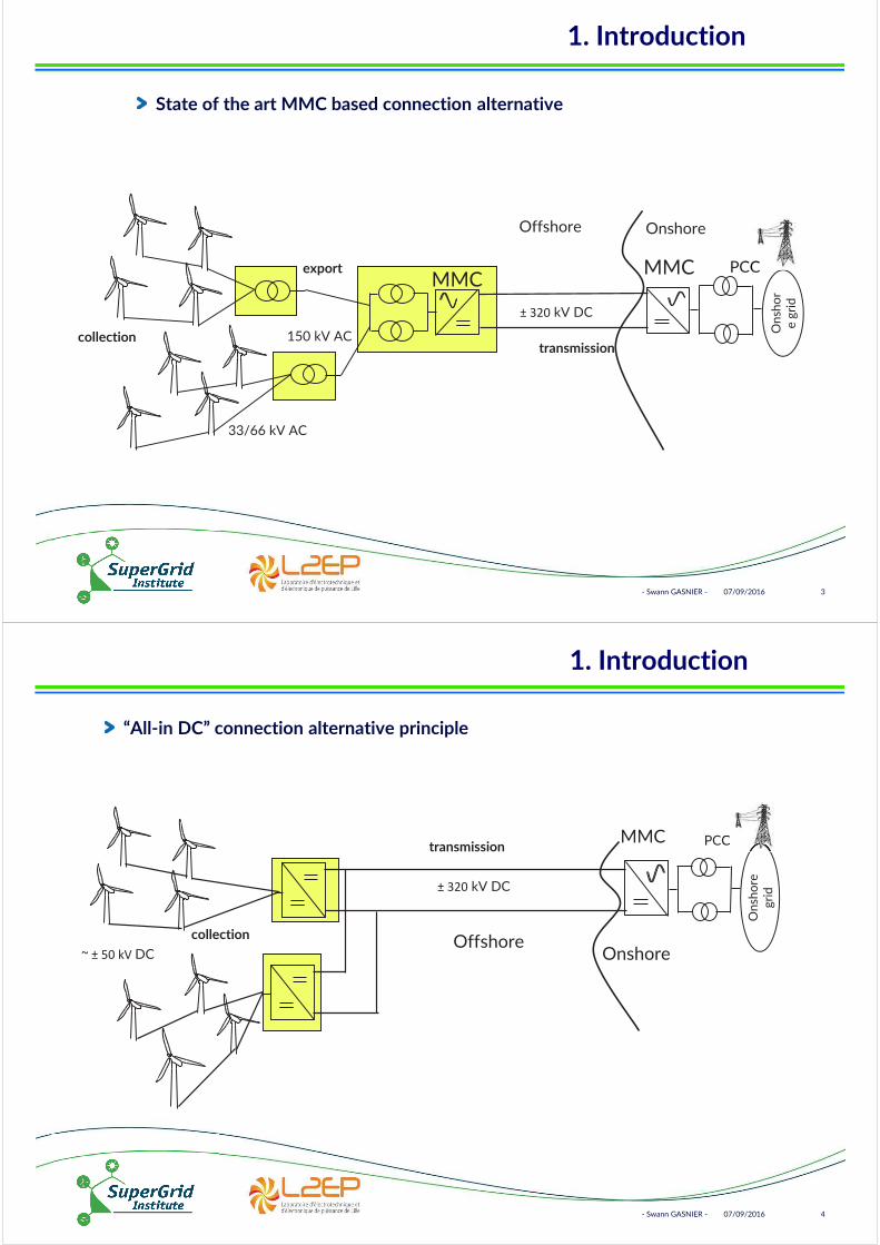
07/09/2016- Swann GASNIER - 3
State of the art MMC based connection alternative
MMCMMC
150 kV AC
33/66 kV AC
± 320 kV DC
Offshore Onshore
PCC
On
sho
re
gri
d
CCexport
collectiontransmission
1. Introduction
07/09/2016- Swann GASNIER - 4
“All-in DC” connection alternative principle
MMC
~ ± 50 kV DC
± 320 kV DC
OffshoreOnshore
PCC
On
sho
reg
rid
C
collection
transmission
1. Introduction

07/09/2016- Swann GASNIER - 5
2. Assessment tool framework
Assessment tool structure
l Given connection
alternative
l Given case study
• Wind farm layout
• Distance to shore
• Wind resources
Inputs
Case studyConnection alternative
Components
data base
07/09/2016- Swann GASNIER - 6
2. Assessment tool framework
Assessment tool structure
l An heuristic designs
the grid system
Inputs
Case studyConnection alternative
Components
data base
Weibull parameters
Design heuristic:
-Select components
-Size selected components
Distance to shoreInstalled power
Technical constraintsAssociation rules
Grid architecture
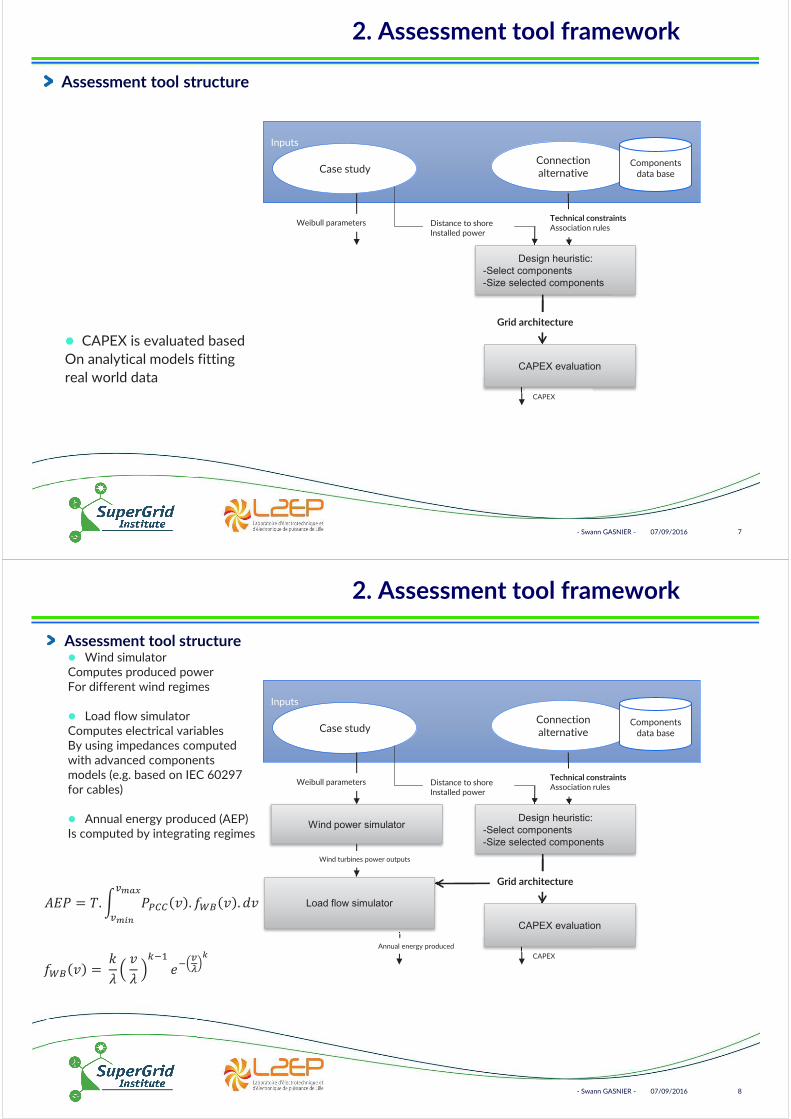
07/09/2016- Swann GASNIER - 7
2. Assessment tool framework
Assessment tool structure
l CAPEX is evaluated based
On analytical models fitting
real world data
Inputs
Case studyConnection alternative
Components
data base
Weibull parameters
Design heuristic:
-Select components
-Size selected components
Distance to shoreInstalled power
CAPEX
Technical constraintsAssociation rules
CAPEX evaluation
Grid architecture
07/09/2016- Swann GASNIER - 8
2. Assessment tool framework
Assessment tool structurel Wind simulator
Computes produced power
For different wind regimes
l Load flow simulator
Computes electrical variables
By using impedances computed
with advanced components
models (e.g. based on IEC 60297
for cables)
l Annual energy produced (AEP)
Is computed by integrating regimes
Inputs
Case studyConnection alternative
Components
data base
Wind power simulator
Wind turbines power outputs
Load flow simulator
Weibull parameters
Design heuristic:
-Select components
-Size selected components
Distance to shoreInstalled power
Annual energy produced
CAPEX
Technical constraintsAssociation rules
CAPEX evaluation
Grid architecture
%$& = 0234567
4589&:;; < 2 >?@ < 2 A<
>?@ < = BC
<C
DE, FE 4G
H

07/09/2016- Swann GASNIER - 9
2. Assessment tool framework
Assessment tool structure
l System criterion (e.g LCOE)
can be computedInputs
Case studyConnection alternative
Components
data base
Wind power simulator
Wind turbines power outputs
Load flow simulator
Weibull parameters
Design heuristic:
-Select components
-Size selected components
Aggregated criterion evaluation
Distance to shoreInstalled power
Annual energy produced
CAPEX
Technical constraintsAssociation rules
Aggregated criterion
(eg. LCOE)
CAPEX evaluation
Grid architecture
!"#$ ="%&$' + ()*,- #)1 + / )
()*,- %$&1 + / )
CAPEX : investment cost
AEP: annual energy produced
Ot :operating cost at year t;
r: discount rate
N: number of years the system is exploited
07/09/2016- Swann GASNIER - 10
2. Assessment tool framework
Assessment tool structure
l Next step is to optimize
The design by guiding heuristic
Inputs
Case studyConnection alternative
Components
data base
Wind power simulator
Wind turbines power outputs
Load flow simulator
Weibull parameters
Design heuristic:
-Select components
-Size selected components
Aggregated criterion evaluation
Distance to shoreInstalled power
Annual energy produced
CAPEX
Technical constraintsAssociation rules
CAPEX evaluation
Grid architecture Optimization
algorithm
Aggregated criterion
(eg. LCOE)
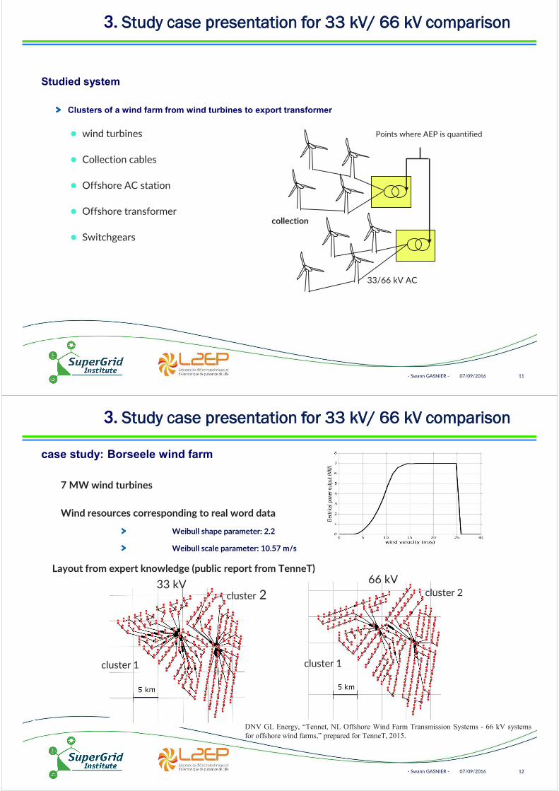
07/09/2016- Swann GASNIER - 11
3. Study case presentation for 33 kV/ 66 kV comparison
Studied system
Clusters of a wind farm from wind turbines to export transformer
l wind turbines
l Collection cables
l Offshore AC station
l Offshore transformer
l Switchgears
33/66 kV AC
collection
Points where AEP is quantified
07/09/2016- Swann GASNIER - 12
3. Study case presentation for 33 kV/ 66 kV comparison
case study: Borseele wind farm
33 kV 66 kV
cluster 1
cluster 2 cluster 2
cluster 1
Layout from expert knowledge (public report from TenneT)
7 MW wind turbines
Wind resources corresponding to real word data
Weibull shape parameter: 2.2
Weibull scale parameter: 10.57 m/s
DNV GL Energy, “Tennet, NL Offshore Wind Farm Transmission Systems - 66 kV systems
for offshore wind farms,” prepared for TenneT, 2015.

07/09/2016- Swann GASNIER - 13
4. Quantitative comparison of 33 kV/ 66 kV
Comparison of total power losses in collection cables
0 100 200 300 400 500 600 700 800
total injected power in cluster 1 (MW)
0
2
4
6
8
10
po
we
r lo
sse
s i
n i
nte
r-a
rra
y c
ab
les (
MW
)
AC 66 kV
AC 33 kV
0 100 200 300 400 500 600 700 800
total injected power in cluster 2 (MW)
0
2
4
6
8
10
po
we
r lo
sse
s i
n i
nte
r-a
rra
y c
ab
les (
MW
)
AC 66 kV
AC 33 kV
ClusterWind turbines Mean annual
produced power (MW)
Wind turbines gross load
factorVoltage level
(kV)
Mean annual inter-array
power losses (MW)
Losses percentage of mean annual
produced power
Cluster 1 335 47.8 % 33 3.77 1.13 %
66 1.98 0.59 %
Cluster 2 335 47.8 % 33 3.62 1.08 %
66 1.90 0.57 %
07/09/2016- Swann GASNIER - 14
4. Quantitative comparison of 33 kV/ 66 kV
CAPEX comparison
Overall system breakdown shows dominant share of wind turbines

07/09/2016- Swann GASNIER - 15
4. Quantitative comparison of 33 kV/ 66 kV
CAPEX comparison
Electrical system CAPEX breakdown
AC 33 kV AC 66 kV0
100
200
300
400
500
600
700
CA
PE
X (
Me
uro
s)
CAPEX breakdown
t ransform ers
AC plat form s
switchgears HV
switchgears MV
collect ion cables
wind turbines increm ental cost
MV cables total cost increase ( - 30 %)Supply cost increase per unit length + 12%
Total length33 kV: 430 km
66 kV: 310 km
MV switchgears total cost increase ( + 100 %)Unitary cost increase + 350 %
Number of feeders/bays33 kV: 40
66 kV: 20
Platform cost decrease (- 2%) due to less feeders (J tubes)
Wind turbine cost increase (encapsulated LV/MV transformer and switchgears)
07/09/2016- Swann GASNIER - 16
4. Quantitative comparison of 33 kV/ 66 kV
Synthesis
0.46 % CAPEX decrease
0.55 % APE increase
0.79 % LCOE increase (9 % discount rate with 20 years life span)Absolute value depend on maintenance costs, taken from The crown Estate public data
Inter-array voltage
(kV)
AEP (GWh)
System CAPEX (M€) LCOE (€/MWh)
33 5785 3655 123.53
66 5817 3638 122.55
« Little brooks make great rivers »
BVG. Associates, “Offshore wind cost reduction pathways Technology work stream,” prepared for The Crown Estate, 2012.

07/09/2016- Swann GASNIER - 17
5. Conclusion
The study confirms the interest of 66 kV collection cables With 7 MW wind turbines, knowing that there are already ratings above
LCOE criterion ?
+ gives information on relative weights of criteria (efficiency, CAPEX)
+ low variation reflects limited energy cost share of studied system
- low sensitivity to electrical connection system technology/design
Ongoing work and prospects on the use of LCC (Life Cycle Cost) equivalent to LCOE
Thank you!
Questions
07/09/2016- Swann GASNIER - 18
![Ille eille aille [eey] ille Fille Famille Gorille Grenouille Papillon Billet.](https://static.fdocuments.net/doc/165x107/551d9db7497959293b8dbf50/ille-eille-aille-eey-ille-fille-famille-gorille-grenouille-papillon-billet.jpg)


![Le son [j] Ier ou iller Il ou ille Ier ou iller Il ou ille.](https://static.fdocuments.net/doc/165x107/551d9d91497959293b8c708b/le-son-j-ier-ou-iller-il-ou-ille-ier-ou-iller-il-ou-ille.jpg)