DI

SC

US

SI

ON

P

AP

ER

S

ER

IE

S

Forschungsinstitut zur Zukunft der ArbeitInstitute for the Study of Labor

Myth or Fact?The Beauty Premium across the Wage Distribution

IZA DP No. 6674

June 2012

Karina DoorleyEva Sierminska

Myth or Fact? The Beauty Premium

across the Wage Distribution

Karina Doorley CEPS/INSTEAD

and University College Dublin

Eva Sierminska CEPS/INSTEAD,

DIW Berlin and IZA

Discussion Paper No. 6674 June 2012

IZA

P.O. Box 7240 53072 Bonn

Germany

Phone: +49-228-3894-0 Fax: +49-228-3894-180

E-mail: iza@iza.org

Any opinions expressed here are those of the author(s) and not those of IZA. Research published in this series may include views on policy, but the institute itself takes no institutional policy positions. The Institute for the Study of Labor (IZA) in Bonn is a local and virtual international research center and a place of communication between science, politics and business. IZA is an independent nonprofit organization supported by Deutsche Post Foundation. The center is associated with the University of Bonn and offers a stimulating research environment through its international network, workshops and conferences, data service, project support, research visits and doctoral program. IZA engages in (i) original and internationally competitive research in all fields of labor economics, (ii) development of policy concepts, and (iii) dissemination of research results and concepts to the interested public. IZA Discussion Papers often represent preliminary work and are circulated to encourage discussion. Citation of such a paper should account for its provisional character. A revised version may be available directly from the author.

IZA Discussion Paper No. 6674 June 2012

ABSTRACT

Myth or Fact? The Beauty Premium across the Wage Distribution*

We apply an innovative technique to allow for differential effects of physical appearance and self-confidence across the wage distribution, as traditional methods can confound opposing effects at either end of the wage distribution. Comparing the effects of beauty and confidence measures in two countries (Germany and Luxembourg), we find that wages are more driven by looks than self-esteem. Counterfactual wage distributions, constructed using distribution regression, show a beauty premium for women at the bottom of the wage distribution. However, most of this is explained by the fact that attractive women have better labor market attributes than their unattractive counterparts. We find a large wage premium for attractive men throughout the wage distribution which is largely unexplained by labor market attributes. There is a small wage penalty for self-confident individuals, particularly men, although their labor market characteristics are generally better than their less confident counterparts. We show that the difference in characteristics between beautiful and plain people contributes to the beauty premium identified using traditional models, particularly for women. Isolating the characteristic effect from the unexplained effect of beauty on wages leads to smaller beauty premium for women. JEL Classification: D31, J24, J30, J70 Keywords: wages, distribution, physical appearance, discrimination Corresponding author: Eva Sierminska CEPS/INSTEAD 3, avenue de la Fonte 4364 Esch-sur-Alzette Luxembourg E-mail: eva.sierminska@ceps.lu

* The authors would like to thank Kevin Denny, Dan Hamermesh, Ronald Oaxaca, Philippe Van Kerm and the participants of the C/I seminar series for helpful suggestions and comments. This research is part of the MeDIM project Advances in the Measurement of Discrimination, Inequality and Mobility supported by the Luxembourg ‘Fonds National de la Recherche’ (contract FNR/06/15/08) and by core funding for CEPS/INSTEAD by the Ministry of Higher Education and Research of Luxembourg.

’All that glitters is not gold’ -W. Shakespeare

1 Introduction

Like in so many areas of life, Shakespeare had excellent insight into the sometimes mis-leading effects of physical appearance. In this paper, we examine whether the glitter ofan appealing physical appearance leads to higher pay across the distribution. We examinetwo type of beauty measures; an interviewer-assessed objective measure of beauty and aself-reported measure, to see whether beauty or ego has an impact on wages. Hamermeshand Biddle (1994), in their seminal paper based on self-reported beauty, show the exis-tence of an average wage penalty of 5-10% for being plain and an average wage premiumof 5-10% for being beautiful in the US and Canada. Most other studies that find a positiveeffect of looks on earnings also identify average effects (Biddle and Hamermesh (1998),Harper (2000), Hamermesh et al. (2002), Mobius and Rosenblat (2006) and Sen et al.(2010)). While measuring average effects is quite informative and convenient, it alsohas substantial drawbacks, as opposing effects that exist across the distribution may beconfounded in the summary effect, as has been discovered for other variables that affectwages, such as gender (Bonjour and Gerfin (2001)).

The effect of beauty on wages throughout the distribution has not been been decomposedinto the part attributable to characteristics and the part due to beauty, or the unobservablesthat beauty proxies. The effect of beauty may vary across the distribution because dif-ferent points of the distribution correspond to different job types, which pay a differentpremium for looks. Better looking people, ceteris paribus, may have more opportunitiesto advance and have higher wages, while less attractive people may need to compensatewith their qualifications and other traits, and the extent of these differences may varydepending on job types and differences in productivity and, consequently, where the indi-vidual is located in the wage distribution. In this paper, our goal is to examine the effectof beauty on earnings across the wage distribution using an innovative technique and newdata.

In studies that use self-assessed beauty as the main explanatory variable one problemis reverse causality, whereby higher-wage people feel better about themselves and, asa result, report that they are better-looking.1 To address this critique, we use a uniquedataset that contains both measures: a self-reported and interviewer-reported objectivemeasure that allows us to disentangle the different effects. To ensure that our analysis isnot subject to further reverse causality, whereby higher wage people with similar othercharacteristics take more care of their appearance due to the extra disposable income, weuse the self-reported measure of beauty as a proxy for confidence in physical appearanceto control for this.

Our contribution to the literature is as follows. First, we demonstrate that the effectof beauty varies across the wage distribution. Second, we use both self-assessed andinterviewer-assessed measures of attractiveness to infer how much of the effect is due tophysical appearance and how much is due to a person’s own assessment of their physical

1Past research indicates better-looking people may actually be more confident before they enter thelabor market (e.g. Persico et al. (2004)) and have other labor market enhancing skills (e.g.Feingold (1992))

2

appearance, or confidence. Third, we devise a classification of occupations based on theimportance of beauty. Fourth, most of the research done on this topic has been for Anglo-Saxon countries. In this paper, we provide evidence for two new countries, Germany andLuxembourg. Finally, we show how distribution regression (DR) a method little used inthis literature and initially used to model excess returns on financial markets, is a usefultool in decomposing wage differentials by physical appearance across the wage distribu-tion. The advantage of the DR method is that, in a flexible and visually appealing way, wecan identify the channel through which beauty (or confidence) affects wages across thedistribution. Do more attractive people have inherently better labor market characteristicsor is there a beauty premium whereby, all else equal, more attractive people earn moremoney, simply because they are attractive or think that they are attractive?

We find that a beauty premium exists at the bottom of the distribution for women andthroughout the distribution for men. This is explained by the fact that attractive womenhave better labor market attributes than their unattractive counterparts. For men this out-come is largely unexplained by labor market attributes.The effect of confidence is am-biguous for women and confident men suffer a wage penalty across the distribution buttheir characteristics are generally better than for their less confident counterparts. Overall,we find that most of the wage differences between confident and unconfident individualsare due to characteristics. We show that the difference in characteristics between beautifuland plain people contributes to the beauty premium identified using traditional models,particularly for women. Isolating the characteristic effect from the unexplained effect ofbeauty on wages leads to smaller beauty premium for women.

In section 2 we provide some background information on prior modeling of the effect ofphysical appearance on various outcome variables and the previous literature. Section 3describes the data and variable construction. In Section 4 we outline our methodology.Sections 5 and 6 discuss the results and Section 7 concludes.

2 Background

Biddle and Hamermesh (1998), Harper (2000), Hamermesh et al. (2002), Mobius andRosenblat (2006) and Sen et al. (2010), using different methods, all find evidence of apositive relationship between physical appearance and earnings.2 This relationship hasbeen shown to be different for men and women and to vary by country. There is a signif-icant effect only for women in the United States (e.g. French (2002)) and only for menin Australia (e.g. Leigh and Borland (2012)) and within professions (Biddle and Hamer-mesh (1998), Sachsida et al. (2003)). A theoretical framework on this issue is offeredby Jackson (1992). In her model, both the sociobiological (reproductive potential) andsociocultural (cultural values) perspectives predict that physical attractiveness has greaterimplications for females than males. Interestingly, despite the increased prevalence ofanti-discrimination legislation, the return to beauty has beauty has been found to be stablein Australia over the last thirty years Leigh and Borland (2012).

There are a number of possible explanations for the relationship between physical appear-ance and earnings. These have been categorized into direct and indirect effects. Direct

2For a recent summary of the literature see Hamermesh (2011).

3

effects, first elaborated by Hamermesh and Biddle (1994), include pure employer dis-crimination, customer discrimination and occupational crowding. The indirect effects areharder to pin down but a number of theories have been put forward. Mocan and Tekin(2010) find evidence that being an unattractive student in high school may hinder humancapital development, due to preferential treatment of attractive students. This will have aknock-on effect on earnings later in life. Mobius and Rosenblat (2006) examine differentchannels through which beauty may affect wages and identify the stereotype channels andtaste-based discrimination.

In a series of other papers, researchers have examined whether there is interviewer baseddiscrimination in favor of better-looking people (e.g. Marlowe et al. (1996), Watkins andJohnston (2000), Lopez Boo et al. (2012)) and find that more attractive people receivemore favorable treatment.

3 Data and Descriptives

We use data for Germany and Luxembourg in our analysis. The 2008 German SocialSurvey contains a unique set of variables on physical appearance: interview-assessedand self-reported physical appearance of the respondent. For Luxembourg, we rely onquestions from the physical discrimination module of the 2007 wave of PSELL3/EU-SILC. Here, our main variables of interest are the respondent’s opinion of how importantphysical appearance is in the labor market, their self-assessed physical appearance andtheir hourly wages.

3.1 Beauty Categories

Given the issue of reverse causality between beauty and wages mentioned in the intro-duction, we will emphasize the distinction between self-reported and objective measuresof beauty and our main results will relate to the effect of beauty (interviewer reported) onwages in Germany, after controlling for confidence (self reported).

We define attractiveness based on the interviewer-assessed objective measure of beautyand confidence based on the self-reported measure of beauty. We take advantage of sev-eral questions.

In the Luxembourg questionnaire, the question is about self-assessed beauty:

Considering now your general physical appearance (height, corpulence, color of the skin,face, etc.). On a scale of 1 to 10, 1 being ‘very little attractive’ and 10 being ’very attrac-tive’ how do you think people around you rate your physical appearance (in comparisonto others of the same age and sex)?

We use this question to create 2 categories of confidence: above and under average. Weexamine the response behavior for this variable by age and gender and find the meanto be 6.5 and the median to be 7. Consequently we define an individual to have aboveaverage confidence if the variable equals 7-10, and below average confidence if it equals1-6.3 We treat proxy respondents, i.e. those who answered this question for somebody

3Hamermesh (2012) finds that absolute rather than relative measures have a greater impact on labor

4

else in the household, separately4 and classify these responses as objective measures ofbeauty, although we treat this as a crude objective measure as it could be confounded bythe relationships that the proxy may have with the respondent. The mean of this variableis 7.3 while the median is 7. Therefore, we define above average beauty as a response of8-10 and below average as a response of 1-7.

In Germany, the interviewer is asked at the beginning and at the end of the interview:Please assess the attractiveness of the respondent. Please come to a spontaneous decision.This is on a scale of 1 to 11, where 1 is ’unattractive and 11 ’attractive’. We interpretthis as an objective measure of beauty. The respondent is also asked to assess their ownphysical appearance on the same scale. We interpret this subjective measure as confi-dence.5 The mean and median response is 7 for confidence and 7.7 and 8 respectively,for objective beauty. Consequently, we define an individual as being attractive if the ob-jective variable equals 8-11, and unattractive if it equals 1-7. The individual is classed asconfident if the subjective variable equals 7-11 and unconfident otherwise.

Based on this classification, in table 1, we find that working women and men are equallylikely to report above and below average beauty and confidence for both types of mea-sures in Luxembourg and Germany. There is a slight statistically significant difference inGermany for the beauty measure, with women being more likely to report better looks.

3.2 Occupation: Dressy and Non-dressy

Hamermesh and Biddle (1994) hypothesize that people sort into occupations where phys-ical appearance may affect productivity. To identify these occupations, we take advantageof a question in the special discrimination module in Luxembourg regarding the role ofbeauty in the work place: Do you think that the physical appearance (height, corpulence,color of the skin, face, etc.) plays an important role in the professional life and the career?The answer is on a 1-5 scale (very important, important, of little importance, not impor-tant, no opinion). We use this question to construct two types of occupation categoriesbased on the role of looks: dressy or non-dressy.

The perceived importance of physical appearance in each of the occupations can be foundin Figure A1. In the non-dressy category we include occupations where, either mostpeople reported looks as unimportant or the job does not entail a lot of people interaction.This category includes farm workers, artists and crafts people, machine operators andblue-collar workers. In all of these occupations people are more likely to state that looksare "not important" than that they are "very important." The dressy occupation categoryincludes occupations where human interaction is an important component of day to dayactivities. These include supervisors and managers, intellectual professions, intermediateprofessions, administrative employees and service and sales employees. We use the sameoccupational classification in Germany. The outcome of these classification can be found

market outcomes.4In a previous version of the paper we did not find any significant effect on wages of having a proxy

respondent (Doorley and Sierminska (2011)).5The correlation between the self-reported and objective measure is 0.3260, which implies that about

10% (0.3262) of the variation in self-reported beauty is related to the variation in objective beauty, which isquite low.

5

in Table 1 bottom panel, which shows that looks are indeed perceived as being moreimportant in the dressy occupation category than in the non-dressy category. We alsoobserve a statistically significant higher concentration of attractive and confident peoplein the dressy profession for both countries (results available from authors).

3.3 Sample, Dependent variable and Covariates

In our sample, we focus on 18 to 64 year olds. We exclude those who work more than onejob, the self-employed and all those who work over 70 hours per week. In Luxembourg,we are left with a sample of 2939 women (1578 workers) and 2837 men (2180 work-ers). From this sample we have measures of objective beauty (confidence) for 428 (2511)women and 809 (2029) men. In Germany, we have 1220 women (795 workers) and 1,198men (910 workers) for whom we have information on objective beauty and confidence.

The explanatory variables used to model wages include education, work experience,6

nationality, marital status, health and job characteristics (dressy profession, temporary,part-time, civil servant, company size). For summary statistics relating to these variables,see Tables A1 and A2.

Comparing hourly wages across various beauty categories in Table 2 indicates that at-tractive men and women report higher wages in Germany. Confident women also reporthigher wages in Germany. In Luxembourg, there is no statistically significant variation inwages between individuals with low and high confidence although attractive men seem tohave lower wages.

Looking at the dressy and non-dressy occupation categories separately in the same table,we find that, contrary to our expectation, there is no correlation between attractivenessor confidence and wages in the dressy profession. Attractive and confident people, in thenon-dressy profession however, report higher wages in Germany.

To summarize, raw wages indicate that there exists a beauty premium for women andmen in Germany, overall and in the non-dressy profession and a confidence premium forfemales overall, and in the non-dressy profession. Men in Luxembourg seem to suffer awage penalty for being attractive. Naturally, it may be the case that good looking individ-uals are better qualified or have other desirable human capital traits and this is the mainreason they obtain a higher wage. In the next section, we extend our analysis to control forthese observable characteristics with both a simple selection model and a more flexibledecomposition methodology.

4 Methodology

We first estimate a Heckman selection model for wages to identify the average effect ofattractiveness and confidence on wages. Next, we use distribution regression (DR) to seehow this changes across the wage distribution and to decompose the effect into a partattributable to characteristics and an unexplained part.

6Due to the availability of other exogenous variables we were able to omit experience from our wageequation in Germany. Neal and Johnson (1996) and others argue that such choice variables should beexcluded when examining discrimination as they themselves may be affected by looks and confidence.

6

4.1 Empirical specification

Our empirical model builds upon Hamermesh and Biddle (1994) (HB) and Mobius andRosenblat (2006) (MR). Our wage function for individual i is expressed in the followingway:

wi = β0 +β1xi +β2Bi +β′2Ci +β3Di +β4BiDi +β

′4CiDi + εi (1)

Bi is a vector indicating whether individual i is physically attractive or not; Ci is a vectorindicating whether individual i is confident or not; Di is an indicator variable for whetherperson i is in an occupation where looks could enhance productivity and zero otherwise(see Section 3.2 for the classification); xi is a vector of other individual level characteris-tics; and εi is the error term.

The situation where we find a robust effect of beauty and/or confidence on earnings,independent of occupations (β2,β

′2 > 0 and β3 = β′3 = β4 = β′4 = 0) could be the result

of employer discrimination or be a stereotype effect whereby attractiveness/confidencehas raised the social and communication skills of good looking people 7 and, as a result,raises employers estimates of workers productivity.

In the HB model, the occupational sorting hypotheses suggests that occupational require-ments for beauty create independent effects on wages and, as a result, lead people to selectcertain occupations based on their looks and the expected returns to those looks. In ourmodel β3,β

′3 > 0 can be interpreted as this occupational sorting, although it can also be

an occupational premium independent of physical appearance.

Finally, workers may sort into occupations where attractiveness pays off (β4,β′4 > 0 and

β2 = β′2 = β3 = β′3 = 0). In this case, physical appearance or confidence therein mayenhance the worker’s ability to engage in productive interactions with coworkers or cus-tomers in certain occupations because they prefer interacting with better looking individ-uals. In this framework there will be a premium for good looks. Attractive and unattrac-tive workers may be in the same occupation if the unattractive worker also has otherproductivity enhancing characteristics that affect the wage. This is known as customerdiscrimination in HB.

We use equation 1 as the basis of our empirical analysis. As a first step, we estimatethe two-step model to correct for selection into work, separately for men and women.P(E = 1|Z) = Φ(Zγ) is the probability that an individual will be employed (E = 1 ifemployed and 0 otherwise). Z is a vector of characteristics that affect the probability ofbeing employed and Φ is the cumulative normal distribution function. Then w∗ is thepotential wage and is not observed if E = 0

w∗= Y β+u (2)

where Y is a vector of characteristics influencing wages (such as company size, contracttype, nationality, education, experience, public sector, occupation type, beauty and confi-dence). Then the expected wage, assuming that the error term in the selection equation, ε

7Research finds that teenagers with wage boosting physical characteristics have higher income as adults(e.g. height in Persico et al. (2004)) suggesting wage enhancing social skills, such as confidence are ac-quired even before individuals enter the labor market.

7

and u, are jointly normal is

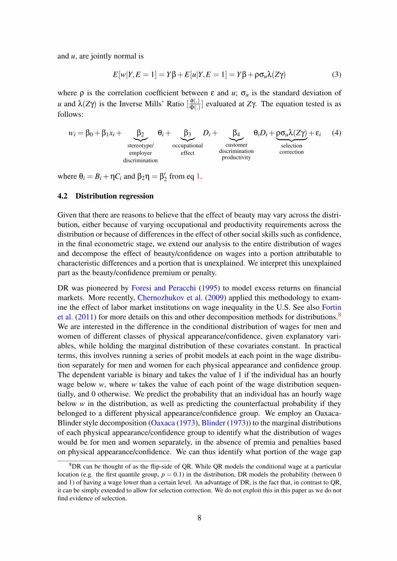
E[w|Y,E = 1] = Y β+E[u|Y,E = 1] = Y β+ρσuλ(Zγ) (3)

where ρ is the correlation coefficient between ε and u; σu is the standard deviation ofu and λ(Zγ) is the Inverse Mills’ Ratio [ φ(.)

Φ(.) ] evaluated at Zγ. The equation tested is asfollows:

wi = β0 +β1xi + β2︸︷︷︸stereotype/employer

discrimination

θi + β3︸︷︷︸occupational

effect

Di + β4︸︷︷︸customer

discriminationproductivity

θiDi +ρσuλ(Zγ)︸ ︷︷ ︸selectioncorrection

+ εi (4)

where θi = Bi +ηCi and β2η = β′2 from eq 1.

4.2 Distribution regression

Given that there are reasons to believe that the effect of beauty may vary across the distri-bution, either because of varying occupational and productivity requirements across thedistribution or because of differences in the effect of other social skills such as confidence,in the final econometric stage, we extend our analysis to the entire distribution of wagesand decompose the effect of beauty/confidence on wages into a portion attributable tocharacteristic differences and a portion that is unexplained. We interpret this unexplainedpart as the beauty/confidence premium or penalty.

DR was pioneered by Foresi and Peracchi (1995) to model excess returns on financialmarkets. More recently, Chernozhukov et al. (2009) applied this methodology to exam-ine the effect of labor market institutions on wage inequality in the U.S. See also Fortinet al. (2011) for more details on this and other decomposition methods for distributions.8

We are interested in the difference in the conditional distribution of wages for men andwomen of different classes of physical appearance/confidence, given explanatory vari-ables, while holding the marginal distribution of these covariates constant. In practicalterms, this involves running a series of probit models at each point in the wage distribu-tion separately for men and women for each physical appearance and confidence group.The dependent variable is binary and takes the value of 1 if the individual has an hourlywage below w, where w takes the value of each point of the wage distribution sequen-tially, and 0 otherwise. We predict the probability that an individual has an hourly wagebelow w in the distribution, as well as predicting the counterfactual probability if theybelonged to a different physical appearance/confidence group. We employ an Oaxaca-Blinder style decomposition (Oaxaca (1973), Blinder (1973)) to the marginal distributionsof each physical appearance/confidence group to identify what the distribution of wageswould be for men and women separately, in the absence of premia and penalties basedon physical appearance/confidence. We can thus identify what portion of the wage gap

8DR can be thought of as the flip-side of QR. While QR models the conditional wage at a particularlocation (e.g. the first quantile group, p = 0.1) in the distribution, DR models the probability (between 0and 1) of having a wage lower than a certain level. An advantage of DR, is the fact that, in contrast to QR,it can be simply extended to allow for selection correction. We do not exploit this in this paper as we do notfind evidence of selection.

8

between groups is due to different characteristics, and what part is unexplained and can,therefore, be attributed to attractiveness or confidence.

Starting from estimates of the conditional distribution of the wages of females or males(s = m, f ) with group characteristics i (i=beautiful (b), plain (p), confident (c) and uncon-fident (u)), given human capital characteristics (x), we recover estimates of the marginaldistribution by integration of the conditional distributions over human capital characteris-tics:

Fs,is,i (w) =

∫Ωx

Fs,i(w|x)hs,i(x)dx (5)

where Fs,i(·|x) is the conditional cumulative wage distribution function for human capitalcharacteristics x in group i and hs,i is the density distribution of human capital character-istics for this group.

Separating marginal wage distributions and human capital distributions in this way al-lows us to define counterfactual wage distributions. For example, we can construct thecounterfactual wage distribution of plain women if they were paid as beautiful women:

F f ,bf ,p (w) =

∫Ωx

F f ,b(w|x)h f ,p(x)dx (6)

where F f ,b(·|x) is the conditional cumulative wage distribution function for beautifulwomen with human capital characteristics x and h f ,p is the density distribution of humancapital characteristics for plain women.

Estimates are obtained by replacing F f ,b(·|x) by estimates F f ,b(·|x) in equation (6), andby averaging over our sample of N plain female workers:

F f ,bf ,p (w) =

N f ,p

∑t=1

F f ,b(w|xt) (7)

Thus the wage gap between plain and beautiful (or unconfident and confident) individ-uals can be decomposed into a part attributable to characteristics and an unexplainedpart, which is the beauty or confidence premium/penalty and is due to different returnsto characteristics for beautiful and plain individuals and for confident and not confidentindividuals. For example:

Fs,ps,p (w)−Fs,b

s,b (w) = [Fs,ps,p (w)− Fs,b

s,p (w)]+ [Fs,bs,p (w)− Fs,b

s,b (w)] (8)

The first expression on the right hand side of equation 8 identifies the unexplained differ-ence between plain and beautiful individuals’ wage distributions. A positive value wouldindicate that there is a premium to being beautiful at wage w. The second expressionidentifies the characteristic effect, which gives the difference in the marginal distributionthat is due to the fact that beautiful and plain individuals have different human capitalcharacteristics. A positive value would indicate that beautiful individuals have better hu-man capital and labor market characteristics than plain individuals since they have a lowerprobability of having a wage below w. We perform this decomposition analogously for

9

unconfident and confident individuals.

5 Empirical Results

In the first instance, we examine the determinants of earnings and check for selection inour model. Next, we test our model described in Section 4. Finally, we use DR techniquesto identify the characteristic and unexplained gaps across the distribution.

5.1 Mean effects of beauty and confidence

Tables 3 to 6 provide results on the selection model for women and men with beautyand confidence measures and on the testing of equation (1), first for Germany and thenLuxembourg. First, we look at the estimation results of the selection equation (columns(3), (6) and (9)). We see that married women and people with bad health are less likelyto work. Age has the traditional positive effect on work for both sexes at a decreasingrate and the number of children has a negative effect on labor supply in both countries. InGermany, we find that the "old-fashioned" variable (Do you believe a woman’s place is inthe home?) has a strong negative effect on the work decision for women while a workingspouse has a significant effect on the working decision of men. In both countries, ρ is notsignificantly different from zero and the low χ2 implies that there is no correlation acrossthe selection probit and wage equation, suggesting that we do not need to worry abouthaving biased estimates if we do not control for selection. We have also included a modelwithout selection in the first column and we find the coefficients to be almost identical inboth models and the R2 to be in the range of 0.25−0.27 for Germany and 0.57−0.63 forLuxembourg in the models without selection correction.

When we look at the direct effects of covariates in the wage equation, we find that maritalstatus has no significant effect on women’s wages (only on the decision to work). Higheducation, experience (in Luxembourg), working for a big company and being a civilservant have the expected positive effects in both countries. Having a temporary workcontract has a diminishing effect on wages in Luxembourg (not available in Germany).We find that working part-time has a positive effect on hourly wages (particularly forwomen). In Luxembourg, both male and female Portuguese immigrants and other non-natives have a disadvantage in the labor market.9 We do not find this to be the case inGermany.

As discussed in Section 3 and Table 2, raw differences indicate that there exists a sta-tistically significant wage penalty for plain workers. When we control for demographicand labor market characteristics, we still find this to be the case in Germany. In Table 3we find a 25% premium for beautiful women (col(2)) and a 17% premium for confidentwomen in Germany. For men, the effect is a little smaller: 16% premium for beauty andno significant effect for confidence. However, when we control for both beauty and con-fidence (col(8)), confidence becomes insignificant for men and women, indicating that itis predominantly through the objective beauty channel that physical appearance affects

9Over 40% of the population in Luxembourg is foreign born with 16.2% born in Portugal. The immi-grant population is an interesting mix of either very low or very high qualified individuals. For a comparativeperspective of immigrants in Luxembourg see Mathae et al. (2011).

10

wages. In Luxembourg, the effect of beauty and confidence on wages is smaller and in-significant. As the Luxembourgish data contains only one of either beauty or confidencefor each observation, we cannot control for both simultaneously.10

Customers may prefer interacting with better looking or more confident individuals em-ployed in certain occupations. In our model this effect is seen in the coefficients onthe interaction terms between beauty/confidence and ‘dressy’ occupations (our β4 and β′4from equation (3)). We find the effect for beauty to be negative and statistically significantonly for women indicating that, for women, beauty does not pay off in occupations thatrequire more personal interactions. The interaction is also negative, but not significant formen. In Luxembourg it is positive, but insignificant for both.

Finally, we examine whether or not there is occupational sorting (our β3). The coefficienton the dressy variable is positive and significant for all our specifications for women andfor men. The effect is a stronger in Germany than in Luxembourg (26%− 32% versus16%−20%) indicating that there are higher wages in occuptions where beauty is deemedmore important in both countries. However, as discussed previously, these may simply behigher paying occupations independently of beauty requirements.

In the next section, we compare these effects across the distribution in the two countries.

5.2 Distributional effects of beauty and confidence

Tables 7 and 8 show the coefficients from distribution regression of the hourly wage atone point in the distribution, the median. The explanatory variables used to model wagesare identical to those used in the mean regressions. Importantly, we include confidenceas a regressor when we model wages by physical appearance category and we use beautyas a regressor when modelling wages by confidence category. The interpretation of thesecoefficients is similar to a probit model. For example, the negative coefficient on marriedin (col(1)) of table 7 indicates that married men within the "plain" group are less likelyto be located in the lower half of the wage distribution, that it, marriage has the typicallypositive effect on wages for this group.

Figure 1 shows the marginal wage distributions of each of the groups of workers in bothcountries.11 Looking first to the left-hand side graphs, which depict the Luxembourgwage distributions, we note that, within beauty categories, plain men earn the most, fol-lowed by beautiful men, beautiful women and, finally, plain women. Within confidencecategories, confident men earn the most, followed by unconfident men and confident andunconfident women (whose wage distributions are very close). We see a slightly differentpicture for Germany. Within beauty categories, beautiful men earn the most, followed byplain men, beautiful women and plain women. Within confidence categories, the order-ing is unconfident men, confident men, confident women and unconfident women. In both

10Recall that the Luxembourg questionnaire contains information about self-assessed beauty, i.e. confi-dence, but that a number of these questions were answered by someone other than the the individual (proxyrespondants) and these observations form a crude group of people for whom we have an objective measureof beauty

11To test the model elaborated in Section 4 using the DR methodology, we plot the predicted distributionof wages for each country against the actual distribution and find an excellent fit for our model (resultsavailable upon request).

11

countries, the difference in distributions by beauty categories is larger than the differencein distributions by confidence categories.

5.2.1 Decomposition: an example

In Figure 2, we provide a graphical example of how the marginal distributions illustratedin Figure 1 are decomposed into the part due to characteristics and the unexplained part, asoutlined mathematically in equation 8. F f ,b

f ,b (w), the marginal wage distribution of beauti-ful women, is represented by the line "Beautiful women". The marginal wage distributionof plain women F f ,p

f ,p (w) is represented by the line"Plain women" while F f ,bf ,p (w), "Plain

women paid as beautiful women" shows the counterfactual wage distribution of plainwomen, rewarded for their characteristics in the same way as are beautiful women. Thevertical difference between the "Plain women" and the "Plain women paid as beautifulwomen" curves depicts the difference in wage distributions that is unexplained and can beattributed to beauty. The difference between the "Plain women paid as beautiful women"and "Beautiful women" curves gives the difference in distribution that is accounted for byobserved characteristics (such as education, age, etc.). In this example, it is clear that thecharacteristic gap dominates at the bottom of the distribution while the unexplained gapis more prominent around the middle of the wage distribution. In the next section, for aclearer exposition, we plot the differences between these curves, rather than the curvesthemselves.

5.3 Explained and unexplained wage differences across the distribution

In figures 3 and 4 we plot a set of characteristic and unexplained differences in distribu-tions for women and men, decomposing the wage distributions as explained in the previ-ous section. We compare the results for the two countries to have a better understandingof cross-national differences.

In Figure 3 we see that the wage premium for females in Germany is located at the bottomof the distribution and peaks at around 7ppt. The beauty premium for females in Luxem-bourg is much larger and is also seen toward the bottom half of the distribution. Thecharacteristics gap in Germany indicates that attractive females have better labor marketcharacteristics than unattractive females, particularly at the bottom of the distribution. InLuxembourg, attractive females have worse characteristics than unattractive females atthe bottom of the distribution, although this trend is reversed further up in the distribu-tion. For men, we find that beauty has an ambiguous effect on wages in Luxembourg,but a very large positive effect in Germany, with the beauty premium approaching 15ppttoward the middle of the distribution. In Luxembourg, attractive men have worse labormarket characteristics than unattractive men, while there is no characteristic gap for menin Germany implying, thus, that differences between the wage distribution of attractiveand unattractive men are all unexplained.

When it comes to confidence, the upper left hand panel in in Figure 4 shows that, whilethere is no clear premium or penalty for confident women in Luxembourg, there is apenalty for confident women in Germany in the bottom half of the wage distribution,peaking at around 5ppt. This means that confident women are 5ppt more likely to earn

12

less than average wages than unconfident women with similar characteristics. The char-acteristic gap between confident and unconfident women is ambiguous in Luxembourgand positive at the bottom of the distribution in Germany, meaning that confident womenhave better characteristics than less confident women at the bottom of the wage distribu-tion in Germany. The confidence effect for men in Luxembourg is ambiguous across thedistribution while the confidence effect for German men, like German women, is negativeand larger than the latter throughout the distribution. However, confident German menhave worse characteristics than their less confident counterparts at the bottom of the wagedistribution, while the reverse is true in Luxembourg throughout the distribution.

Trusting the objective beauty measure from the German data more than that from theLuxembourg data, we base our conclusions relating to beauty on this country. We finda beauty premium for both women and men, although that for women is concentratedin the lower half of the wage distribution and is smaller than that for men. Basing ourconclusions about confidence on results from both countries, we find that confidence af-fects wages ambiguously across the wage distribution in Luxembourg but that there arepenalties for confidence in Germany, especially for men.

5.4 A comparison

As suspected, differences exist in the beauty premium estimated using traditional meth-ods (in section 5.1) and those estimated across the wage distribution using decompositiontechniques. Evaluating the effect of beauty on wages at the mean, we find that womenexperience a larger beauty premium (20% in Germany, 10% in Luxembourg) than men(14% in Germany, -3% in Luxembourg). However, when we use decomposition tech-niques to isolate the portion of the beauty premium that is due to different characteristicsbetween groups, we find that, in Germany, attractive men experience a larger unexplainedwage premium than women (see Figure 3) . Much of the beauty premium for women,identified using simple regressions, is therefore due to the characteristic gap between at-tractive and unattractive women (seen in the top right panel of Figure 3). In Luxembourg,the characteristic gap is negative for men, and negative to positive for women as we lookacross the wage distribution. In the case of women, the characteristic gap works in theopposite direction to the unexplained gap throughout the distribution so that failure todecompose the beauty premium into these two components gives misleading results. Formen in Luxembourg, the characteristic gap is negative throughout the distribtution andlarger than the unexplained gap, which results in an overall beauty penalty when we usesimple regression. In every case, the characteristic and unexplained gaps are larger at thebottom of the wage distribution than at the top, reinforcing the importance of looking atthese effects in a distributional context.

6 Robustness checks

As explained in Section 3, the self reported measures that we use to proxy confidence maybe endogenous if people feel more confident or beautiful when they earn more. While itis interesting to see how these self-reported measures compare against objective measuresin Figures 3 and 4, we may not be able to draw any causal inference from them. There-fore next we check the robustness of the objective beauty measure results in Germany.

13

Figure 5 presents the decomposition of the marginal wage distributions in Germany into acharacteristic effect and an unexplained (beauty) effect with fitted 95% confidence inter-vals.12 The small beauty effect observed for women at the bottom of the wage distributionis statistically insignificant, while the beauty premium for men is statistically significantthroughout the distribution. Additionally, the small positive characteristic effect observedfor women is significant at the bottom of the wage distribuition.

As outlined in Section 4.1 our framework suggested the existence of occupational sort-ing whereby looks could enhance productivity and yield a positive effect on wages. Tocheck this prediction, we present results from an additional specification. We retain onlythose who work in the "dressy" profession and rerun our analysis using the distributionregression framework. If sorting is taking place, individuals with less desirable phys-ical appearance characteristics but higher other labor market attributes and those withdesirable physical appearance characteristics but lower other labor market attributes canbe expected to sort into "dressy" professions. In both cases, we would expect to see adownward movement of the characteristic gap. Looking at Figure 6, we see that the char-acteristic gap has gone from positive to zero for women at the bottom of the distributionand from zero to negative for men at the bottom of the distribution. This is in line withour expectations as there are either relatively more ill qualified attractive people or morehighly qualified unattractive people in the dressy profession. Whichever is the case, thisprovides evidence of occupational sorting, based on physical appearance, at the bottomof the wage distribution.

In a further analysis, we restrict the sample to young (18-45 year old) people, whosephysical appearance may be more important in the labor market (Figure 7). For youngmen, we find that the beauty premium is slightly smaller than that of the whole sample(peaking at around 12ppt) and it is more localised at the bottom of the wage distribution.The beauty premium for young women is larger than that of the whole sample (at around11ppt at the bottom of the distribution) but is, once again, concentrated around the bottomof the wage distribution. It seems that, similar to what has been suggested for the Anglo-Saxon countries, beauty influences the wages of young women more and young men lessthan the older cohort. However, due to the small sample size of the younger groups, wesee large confidence intervals. This issue could be alleviated and the results strengthenedwith a larger sample size.

7 Conclusions

Using data from two countries and various techniques, we show that the effect of beautyvaries across the distribution and that mean techniques can provide misleading informa-tion as opposing effects may cancel each other out. We also demonstrate that differencesin observable characteristics between attractive and unattractive people can lead to erro-neous estimates of the effect of beauty on wages using traditional methods.

Given the opportunity of using unique data sets, which contain both subjective and objec-tive measures of beauty, we find that the effect of beauty on wages dominates the effect of

12The confidence intervals are constructed using the point estimates +/- 1.96 standard deviations calcu-lated from 250 draws at the individual level.

14

confidence. There is a beauty premium at the bottom of the wage distribution for womenand throughout the distribution for men. A similar average result has been found for Aus-tralia (Leigh and Borland (2012)), while results from the U.S./Canada tend to find larger(or similar) premia for women than men. The effect of confidence is ambiguous or nega-tive for both women and men across the distribution. This is a new result as both Hamer-mesh and Biddle (1994), for the U.S. and Canada, and Mobius and Rosenblat (2006) forArgentina, find some evidence of confidence wage premia. However, as we find charac-teristic gaps between confident and unconfident women and men (with confident peoplehaving better labor market characteristics for the most part), this result is unsurprising.Indeed, our estimation of mean effects would suggest a positive (although) insigificanteffect of confidence on wages for both men and women. Decomposition techniques showthat this positive effect is largely due to observable characteristic differences between thetwo groups.

Restricting our sample to those working in professions where beauty is deemed more im-portant, we find evidence of occupational sorting by beauty requirements and, restrictingour sample to the young (<45), we find preliminary evidence that beauty may be morerelated to wages for young women than older women. The availability of a larger samplefor the young would allow further research about the effects of beauty on wages for thisgroup, in particular.

By constructing counterfactual distributions using DR, we find that much of the wagepenalties observed in the Hamermesh and Biddle (1994) model are due to the differentcharacteristics of people in different physical appearance classes, and only a small por-tion is actually unexplained and may be attributed to discrimination. The DR method,which is largely unused in this literature, provides a straight forward manner in which todecompose wage distributions into explained and unexplained components, if we suspectthe effect of varying across the distribution.

References

Biddle, J. E. and Hamermesh, D. S. (1998). Beauty, Productivity, and Discrimination:Lawyers’ Looks and Lucre. Journal of Labor Economics, 16(1):172–201. 3, 4

Blinder, A. S. (1973). Wage discrimination: Reduced form and structural estimates. TheJournal of Human Resources, 8(4):pp. 436–455. 9

Bonjour, D. and Gerfin, M. (2001). The unequal distribution of unequal pay - An empiri-cal analysis of the gender wage gap in Switzerland. Empirical Economics, 26(2):407–427. 3

Chernozhukov, V., Fernandez-Val, I., and Melly, B. (2009). Inference on counterfactualdistributions. CeMMAP working papers CWP09/09, Centre for Microdata Methodsand Practice, Institute for Fiscal Studies. 9

Doorley, K. and Sierminska, E. (2011). Beauty and the beast in the labor market: Evi-dence from a distribution regression approach. CEPS/INSTEAD Working Paper Series2011-62, CEPS/INSTEAD. 6

15

Feingold, A. (1992). Good-looking people are not what we think. Psychological Bulletin,111(2):304–41. 3

Foresi, S. and Peracchi, F. (1995). The Conditional Distribution of Excess Returns: AnEmpirical Analysis. Journal of the American Statistical Association, 90(430):pp. 451–466. 9

Fortin, N., Lemieux, T., and Firpo, S. (2011). Decomposition Methods in Economics,volume 4 of Handbook of Labor Economics, chapter 1, pages 1–102. Elsevier. 9

French, M. T. (2002). Physical appearance and earnings: further evidence. AppliedEconomics, 34:569–572. 4

Hamermesh, D. S. (2011). Beauty Pays: Why attractive people are more successful.Princeton University Press. 4

Hamermesh, D. S. (2012). Tall or Taller, Pretty or Prettier: Is Discrimination Absolute orRelative? Working Paper 18123, National Bureau of Economic Research. 5

Hamermesh, D. S. and Biddle, J. E. (1994). Beauty and the Labor Market. AmericanEconomic Review, 84(5):1174–94. 3, 5, 6, 8, 16

Hamermesh, D. S., Meng, X., and Zhang, J. (2002). Dress for success–does primpingpay? Labour Economics, 9(3):361–373. 3, 4

Harper, B. (2000). Beauty, Stature and the Labour Market: A British Cohort Study.Oxford Bulletin of Economics and Statistics, 62:771–800. 3, 4

Jackson, L. (1992). Physical attractiveness: A sociocultural perspective. New York:Guilford. 4

Leigh, A. and Borland, J. (2012). Unpacking the beauty premium: What channels does itoperate through, and has it changed over time?? 4, 16

Lopez Boo, F., Rossi, M. A., and Urzua, S. (2012). The labor market return to an attractiveface: Evidence from a field experiment. IZA Discussion Papers 6356, Institute for theStudy of Labor (IZA). 5

Marlowe, C., Schneider, S., and Carnot, N. (1996). Gender and attractiveness biasesin hiring decisions: are more experienced managers less biased? Journal of AppliedPsychology, 81(1):11–21. 5

Mathae, T. Y., Porpiglia, A., and Sierminska, E. (2011). The immigrant/native wealthgap in Germany, Italy and Luxembourg. Working Paper Series 1302, European CentralBank. 11

Mobius, M. M. and Rosenblat, T. S. (2006). Why beauty matters. American EconomicReview, 96(1)(5):222–35. 3, 4, 5, 8, 16

Mocan, N. and Tekin, E. (2010). Ugly criminals. The Review of Economics and Statistics,Vol. 92, No. 1:Pages 15–30. 5

16

Neal, D. A. and Johnson, W. R. (1996). The role of premarket factors in black-white wagedifferences. Journal of Political Economy, 104(5):869–95. 7

Oaxaca, R. (1973). Male-female wage differentials in urban labor markets. InternationalEconomic Review, 14(3):693–709. 9

Persico, N., Postlewaite, A., and Silverman, D. (2004). The effect of adolescent expe-rience on labor market outcomes: The case of height. Journal of Political Economy,112:1019–1053. 3, 8

Sachsida, A., Dornelles, A. C., and Mesquita, C. W. (2003). Beauty and the labor market- study one specific occupation. 4

Sen, A., Voia, M.-C., and Woolley, F. R. (2010). Hot or not: How appearance affectsearnings and productivity in academia. Carleton Economic Papers 10-07, CarletonUniversity, Department of Economics. 3, 4

Watkins, L. and Johnston, L. (2000). Screening job applicants: The impact of physical at-tractiveness and application quality. International Journal of Selection and Assessment,8(2):76–84. 5

8 Tables and Figures

17

Table 1: A comparison of the beauty and confidence measures for women and men and the per-ceived importance of beauty in Germany and Luxembourg.

Panel ALuxembourg Women Men diffShare in each categoryBeautiful 0.534 0.529 0.005Plain 0.466 0.471 -0.005Confident 0.436 0.450 -0.014Unconfident 0.564 0.550 0.014Germany

Share in each categoryBeautiful 0.593 0.540 0.053∗∗∗

Plain 0.407 0.460 -0.053∗∗∗

Confident 0.603 0.574 0.029Unconfident 0.397 0.426 -0.029Panel BLuxembourg Non-dressy Dressy diffPerceived importance of beauty:All 1.795 1.959 -0.164∗∗∗

Women 1.806 2.041 -0.235∗∗∗

Men 1.789 1.869 -0.080∗∗

Perceived importance of beauty is 1-4 variable with 1: very important and 4: not important

Source: 2008 GSS, 2007 PSELL; t statistics in parentheses * p<0.1 ** p<0.05 *** p<0.01

18

Table 2: Select wage differences statistics for beauty and confidence categories and by occupation(in Euros).

Germany beauty Above Under diffAll 10.974 9.184 1.790∗∗∗

Women 9.621 8.347 1.274∗∗

Men 12.215 9.740 2.476∗∗

Women: Dressy 9.884 9.367 0.517Men: Dressy 13.243 12.099 1.144Women: Non-dressy 8.592 6.111 2.481∗∗∗

Men: Non-Dressy 11.359 8.176 3.183∗

Germany confidence Above Under diffAll 10.555 9.891 0.664Women 9.619 8.410 1.208∗∗

Men 11.394 10.932 0.462Women: Dressy 10.057 9.099 0.958Men: Dressy 12.428 13.639 -1.211Women: Non-dressy 8.128 6.620 1.508∗

Men: Non-Dressy 10.503 9.163 1.341Luxembourg confidence Above Under diffAll 16.093 16.225 -0.133Women 14.973 15.785 -0.812Men 17.087 16.610 0.478Women: Dressy 16.929 18.118 -1.189Men: Dressy 20.402 21.202 -0.800Women: Non-Dressy 8.436 9.386 -0.949Men: Non-Dressy 10.861 11.170 -0.309Luxembourg beauty Above Under diffAll 14.531 15.713 -1.182Women 12.973 11.519 1.454Men 15.051 17.050 -1.999∗∗

Women: Dressy 14.239 13.842 0.397Men: Dressy 19.744 21.999 -2.255∗

Women: Non-Dressy 8.416 7.945 0.471Men: Non-Dressy 10.150 10.985 -0.835Source: 2008 GSS, 2007 PSELL3; t statistics in parentheses * p<0.1 ** p<0.05 *** p<0.01

19

Tabl

e3:

OL

San

dse

lect

ion

mod

elfo

robj

ectiv

e,su

bjec

tive

and

both

beau

tyca

tego

ries

inG

erm

any

(wom

en).

Bea

uty

Con

fiden

ceB

oth

wag

ew

age

wor

kw

age

wag

ew

ork

wag

ew

age

wor

k(1

)(2

)(3

)(4

)(5

)(6

)(7

)(8

)(9

)be

auty

0.25

***

0.25

***

0.20

**0.

20**

beau

ty*d

ress

y-0

.26*

*-0

.26*

*-0

.22*

*-0

.22*

*co

nfide

nt0.

18*

0.17

*0.

120.

12co

nfide

nt*d

ress

y-0

.15

-0.1

5-0

.09

-0.0

9dr

essy

0.32

***

0.32

***

0.26

***

0.26

***

0.34

***

0.34

***

age

0.00

0.00

0.25

***

0.00

0.01

0.25

***

0.00

0.00

0.25

***

age2

0.01

0.01

-0.2

9***

0.00

0.00

-0.2

9***

0.00

0.00

-0.2

9***

no.c

hild

ren

-0.0

1-0

.01

-0.2

7***

-0.0

1-0

.01

-0.2

7***

-0.0

1-0

.01

-0.2

7***

child

0.08

0.08

-0.1

40.

090.

09-0

.14

0.09

0.09

-0.1

4m

arri

ed-0

.05

-0.0

5-0

.26*

-0.0

5-0

.05

-0.2

6*-0

.05

-0.0

5-0

.26*

low

educ

.-0

.10*

*-0

.10*

*-0

.12*

*-0

.12*

*-0

.10*

*-0

.10*

*hi

ghed

uc.

0.29

***

0.29

***

0.29

***

0.29

***

0.29

***

0.29

***

part

-tim

e0.

16**

*0.

16**

*0.

15**

*0.

15**

*0.

15**

*0.

15**

*bi

gco

mpa

ny0.

10**

*0.

10**

*0.

10**

0.10

**0.

09**

0.09

**ci

vils

erva

nt0.

14**

*0.

14**

*0.

13**

*0.

13**

*0.

14**

*0.

14**

*ba

dhe

alth

-0.0

7-0

.07

-0.4

8***

-0.0

8-0

.09

-0.4

9***

-0.0

7-0

.07

-0.4

9***

imm

igra

nt-0

.03

-0.0

3-0

.04

-0.0

4-0

.04

-0.0

4ol

d-fa

shio

ned

-0.3

9***

-0.4

0***

-0.4

0***

wor

king

spou

se0.

060.

060.

06C

onst

ant

1.59

***

1.60

***

-4.3

2***

1.59

***

1.56

***

-4.2

9***

1.51

***

1.49

***

-4.2

9***

λ0.

000.

000.

00ρ

-0.0

10.

010.

01σ

0,43

***

0,43

***

0,43

***

Wal

dte

st(χ

2 ).

0.00

.0.

01.

0.01

Pseu

do-R

20.

250.

230.

24O

bser

vatio

ns58

31,

121

1,12

157

71,

115

1,11

557

71,

115

1,11

5So

urce

:200

8G

erm

anG

ener

alSo

cial

Surv

ey;R

obus

tsta

ndar

der

rors

used

.ts

tatis

tics

inpa

rent

hese

s*

p<0.

1**

p<0.

05**

*p<

0.01

20

Tabl

e4:

OL

San

dse

lect

ion

mod

elfo

robj

ectiv

e,su

bjec

tive

and

both

beau

tyca

tego

ries

inG

erm

any

(men

).

Bea

uty

Con

fiden

ceB

oth

wag

ew

age

wor

kw

age

wag

ew

ork

wag

ew

age

wor

k(1

)(2

)(3

)(4

)(5

)(6

)(7

)(8

)(9

)be

auty

0.16

**0.

16**

0.14

**0.

14**

beau

ty*d

ress

y-0

.11

-0.1

1-0

.09

-0.0

9co

nfide

nt0.

060.

060.

030.

03co

nfide

nt*d

ress

y-0

.08

-0.0

8-0

.06

-0.0

6dr

essy

0.31

***

0.31

***

0.28

***

0.28

***

0.32

***

0.32

***

age

0.01

0.01

0.26

***

0.01

0.01

0.26

***

0.01

0.01

0.26

***

age2

0.00

0.00

-0.3

1***

0.00

-0.0

0-0

.31*

**0.

00-0

.00

-0.3

1***

no.c

hild

ren

0.00

0.00

-0.1

9*0.

010.

01-0

.20*

0.00

0.00

-0.2

0*ch

ild0.

060.

060.

39*

0.04

0.04

0.40

*0.

050.

050.

40*

mar

ried

0.16

***

0.16

***

0.22

0.14

***

0.14

***

0.22

0.13

***

0.14

***

0.22

low

educ

.0.

030.

030.

040.

030.

040.

04hi

ghed

uc.

0.19

***

0.19

***

0.21

***

0.21

***

0.20

***

0.20

***

part

-tim

e0.

53**

*0.

53**

*0.

53**

*0.

53**

*0.

52**

*0.

52**

*bi

gco

mpa

ny0.

20**

*0.

20**

*0.

21**

*0.

21**

*0.

20**

*0.

20**

*ci

vils

erva

nt0.

020.

020.

020.

020.

010.

01ba

dhe

alth

-0.0

6-0

.07

-1.1

4***

-0.0

8-0

.09

-1.1

2***

-0.0

8-0

.09

-1.1

2***

imm

igra

nt0.

010.

010.

030.

030.

040.

04ol

d-fa

shio

ned

-0.1

0-0

.11

-0.1

1w

orki

ngsp

ouse

0.29

**0.

30**

0.30

**C

onst

ant

1.37

***

1.33

***

-4.3

6***

1.40

***

1.35

***

-4.3

6***

1.32

***

1.27

***

-4.3

6***

λ0.

020.

020.

02ρ

0,03

0,03

0,03

σ0.

52**

*0.

52**

*0.

52**

*W

ald

test

(χ2 )

.0.

750

.0.

880

.0.

760

Pseu

do-R

20.

260.

260.

27O

bser

vatio

ns71

91,

044

1,04

470

31,

028

1,02

870

31,

028

1,02

8So

urce

:200

8G

erm

anG

ener

alSo

cial

Surv

ey;R

obus

tsta

ndar

der

rors

used

.ts

tatis

tics

inpa

rent

hese

s*

p<0.

1**

p<0.

05**

*p<

0.01

21

Tabl

e5:

OL

San

dse

lect

ion

mod

elfo

rsub

ject

ive

and

prox

ybe

auty

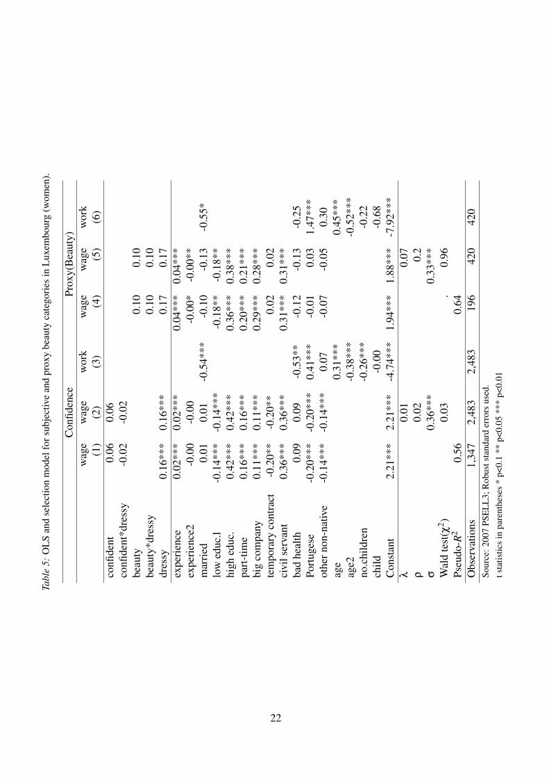
cate

gori

esin

Lux

embo

urg

(wom

en).

Con

fiden

cePr

oxy(

Bea

uty)

wag

ew

age

wor

kw

age

wag

ew

ork

(1)

(2)

(3)

(4)

(5)

(6)

confi

dent

0.06

0.06

confi

dent

*dre

ssy

-0.0

2-0

.02

beau

ty0.

100.

10be

auty

*dre

ssy

0.10

0.10

dres

sy0.

16**

*0.

16**

*0.

170.

17ex

peri

ence

0.02

***

0.02

***

0.04

***

0.04

***

expe

rien

ce2

-0.0

0-0

.00

-0.0

0*-0

.00*

*m

arri

ed0.

010.

01-0

.54*

**-0

.10

-0.1

3-0

.55*

low

educ

.l-0

.14*

**-0

.14*

**-0

.18*

*-0

.18*

*hi

ghed

uc.

0.42

***

0.42

***

0.36

***

0.38

***

part

-tim

e0.

16**

*0.

16**

*0.

20**

*0.

21**

*bi

gco

mpa

ny0.

11**

*0.

11**

*0.

29**

*0.

28**

*te

mpo

rary

cont

ract

-0.2

0**

-0.2

0**

0.02

0.02

civi

lser

vant

0.36

***

0.36

***

0.31

***

0.31

***

bad

heal

th0.

090.

09-0

.53*

*-0

.12

-0.1

3-0

.25

Port

uges

e-0

.20*

**-0

.20*

**0.

41**

*-0

.01

0.03

1.47

***

othe

rnon

-nat

ive

-0.1

4***

-0.1

4***

0.07

-0.0

7-0

.05

0.30

age

0.31

***

0.45

***

age2

-0.3

8***

-0.5

2***

no.c

hild

ren

-0.2

6***

-0.2

2ch

ild-0

.00

-0.6

8C

onst

ant

2.21

***

2.21

***

-4.7

4***

1.94

***

1.88

***

-7.9

2***

λ0.

010.

07ρ

0.02

0.2

σ0.

36**

*0.

33**

*W

ald

test

(χ2 )

0.03

.0.

96Ps

eudo

-R2

0.56

0.64

Obs

erva

tions

1,34

72,

483

2,48

319

642

042

0So

urce

:200

7PS

EL

L3;

Rob

usts

tand

ard

erro

rsus

ed.

tsta

tistic

sin

pare

nthe

ses

*p<

0.1

**p<

0.05

***

p<0.

01

22

Tabl

e6:

OL

San

dse

lect

ion

mod

elfo

rsub

ject

ive

and

prox

ybe

auty

cate

gori

esin

Lux

embo

urg

(men

).

Con

fiden

cePr

oxy

(Bea

uty)

wag

ew

age

wor

kw

age

wag

ew

ork

(1)

(2)

(3)

(4)

(5)

(6)

confi

dent

0.01

0.01

confi

dent

*dre

ssy

-0.0

1-0

.01

beau

ty-0

.03

-0.0

3be

auty

*dre

ssy

0.09

0.09

dres

sy0.

20**

*0.

20**

*0.

20**

*0.

20**

*ex

peri

ence

0.03

***

0.03

***

0.03

***

0.03

***

expe

rien

ce2

-0.0

0***

-0.0

0***

-0.0

0***

-0.0

0***

mar

ried

0.05

0.05

0.20

0.12

**0.

12**

low

educ

.-0

.22*

**-0

.22*

**-0

.09*

-0.0

9*hi

ghed

uc.

0.35

***

0.35

***

0.42

***

0.42

***

part

-tim

e0.

36**

*0.

36**

*0.

130.

14bi

gco

mpa

ny0.

15**

*0.

15**

*0.

19**

*0.

19**

*te

mpo

rary

-0.1

9***

-0.1

9***

-0.1

9**

-0.1

9**

civi

lser

vant

0.26

***

0.26

***

0.27

***

0.27

***

bad

heal

th-0

.05

-0.0

6-1

.74*

**-0

.18*

**-0

.15*

*-2

.24*

**Po

rtug

ese

-0.2

1***

-0.2

1***

0.38

*-0

.23*

**-0

.23*

**0.

78**

othe

rnon

-nat

ive

-0.1

3***

-0.1

3***

0.03

-0.1

4***

-0.1

4***

0.04

age

0.46

***

0.57

***

age2

-0.5

8***

-0.6

9***

no.c

hild

ren

0.02

-0.3

2**

child

0.07

0.74

**C

onst

ant

2.30

***

2.29

***

-7.3

2***

2.19

***

2.22

***

-9.4

9***

λ0.

01-0

.05

ρ0.

02-0

.35

σ0,

33**

*0,

30**

*W

ald

test

(χ2 )

..0

10.

0.48

3Ps

eudo

-R2

0.63

0.65

Obs

erva

tions

1,53

32,

000

2,00

059

478

278

2So

urce

:200

7PS

EL

L3;

Rob

usts

tand

ard

erro

rsus

ed.

tsta

tistic

sin

pare

nthe

ses

*p<

0.1

**p<

0.05

***

p<0.

01

23

Tabl

e7:

Dis

trib

utio

nre

gres

sion

atth

em

edia

nw

age

forG

erm

any

bybe

auty

orco

nfide

nce

cate

gory

(1)

(2)

(3)

(4)

(5)

(6)

(7)

(8)

VAR

IAB

LE

SPl

ain

Plai

nB

eaut

iful

Bea

utif

ulU

ncon

fiden

tU

ncon

fiden

tC

onfid

ent

Con

fiden

tm

ale

fem

ale

mal

efe

mal

em

ale

fem

ale

Mal

efe

mal

e

age

-0.0

9-0

.12

-0.0

5-0

.00

-0.0

3-0

.05

-0.0

7-0

.01

age2

0.00

0.00

0.00

-0.0

00.

000.

000.

00-0

.00

mar

ried

-0.8

5***

0.27

-0.4

8**

0.26

-0.5

3**

0.01

-0.6

7***

0.37

**ch

ild-0

.32

-0.5

40.

06-0

.28

0.15

-0.2

8-0

.11

-0.5

2*no

.chi

ldre

n0.

220.

10-0

.06

0.03

-0.0

2-0

.07

0.03

0.17

low

educ

.-0

.53*

*0.

40-0

.20

0.02

-0.5

3**

0.36

-0.3

00.

03hi

ghed

uc.

-0.3

2-0

.22

-0.6

3***

-0.8

9***

-0.8

3***

-0.4

2*-0

.35*

*-0

.80*

**ba

dhe

alth

0.21

0.34

0.17

0.03

0.32

0.12

0.08

0.29

imm

igra

nt0.

100.

010.

080.

150.

430.

180.

190.

05pa

rt-t

ime

-1.2

0-0

.49*

*-0

.69

-0.2

1-0

.28

-0.2

2-1

.42*

*-0

.36*

*bi

gco

.-0

.53*

**-0

.16

-0.7

7***

-0.2

9*-0

.77*

**-0

.11

-0.6

1***

-0.2

9*ci

vils

erva

nt0.

10-0

.09

-0.2

2-0

.11

-0.2

1-0

.06

-0.0

3-0

.14

dres

sy-1

.27*

**-0

.64*

**-0

.44*

**-0

.27

-0.8

5***

-0.8

4***

-0.7

2***

-0.2

1co

nfide

nt0.

23-0

.13

0.06

-0.1

7be

autif

ul-0

.07

0.19

-0.1

80.

03co

nsta

nt3.

12**

4.00

**2.

02*

1.54

1.93

2.59

*2.

79**

*1.

48

Obs

erva

tions

316

214

402

372

296

208

422

378

Rob

usts

tand

ard

erro

rsin

pare

nthe

ses

***

p<0.

01,*

*p<

0.05

,*p<

0.1

24

Tabl

e8:

Dis

trib

utio

nre

gres

sion

atth

em

edia

nw

age

forL

uxem

bour

gby

beau

tyor

confi

denc

eca

tego

ry

(1)

(2)

(3)

(4)

(5)

(6)

(7)

(8)

VAR

IAB

LE

SPl

ain

Plai

nB

eaut

iful

Bea

utif

ulU

ncon

fiden

tU

ncon

fiden

tC

onfid

ent

Con

fiden

tm

ale

fem

ale

mal

efe

mal

em

ale

fem

ale

Mal

efe

mal

e

age

-0.4

5***

0.03

0.00

0.31

**-0

.02

-0.2

2***

-0.2

9***

-0.2

4***

age2

0.00

***

-0.0

0-0

.00

-0.0

1***

-0.0

00.

00**

0.00

***

0.00

**m

arri

ed0.

250.

52-1

.46*

**-0

.35

-0.5

6**

-0.2

3-0

.38*

*-0

.41*

*ch

ild-1

.12*

-0.6

5-0

.06

2.02

**-0

.57

-0.5

6*0.

04-0

.07

no.c

hild

ren

0.20

0.79

**0.

08-0

.96*

*0.

28**

0.24

*-0

.05

0.12

low

educ

.0.

75**

0.28

0.53

2.25

***

0.92

***

-0.0

10.

63**

0.10

high

educ

.-0

.86*

*-1

.46*

**-0

.67

-1.2

3*-0

.22

-1.2

7***

-0.3

6-0

.86*

**ba

dhe

alth

1.54

***

1.65

*1.

56**

*-0

.90*

0.37

1.00

**po

rtug

uese

0.79

**0.

461.

51**

*0.

260.

85**

*0.

520.

55*

1.46

***

part

-tim

e-0

.16

-0.7

0-0

.97*

-1.0

8-0

.57*

*-0

.53*

*0.

50-0

.21

big

co.

-0.6

3**

-1.1

8***

-0.5

1*-2

.73*

**-0

.28

-0.5

0***

-0.7

7***

-0.2

6ci

vils

erva

nt-1

.51*

**0.

18-1

.68*

**-1

.04

-1.3

8***

-1.4

9***

-1.4

0***

-0.6

3**

dres

sy-0

.62*

-2.4

1***

-0.7

3**

-0.3

8-0

.63*

**-1

.07*

**-0

.37*

-0.4

8co

nsta

nt10

.21*

**4.

011.

91-2

.57

1.70

7.07

***

7.09

***

6.10

***

Obs

erva

tions

331

108

258

8572

662

980

771

8R

obus

tsta

ndar

der

rors

inpa

rent

hese

s**

*p<

0.01

,**

p<0.

05,*

p<0.

1

25

Figure 1 Marginal wage distribution functions

Note: Predicted marginal wage distributions for men and women grouped by beauty andconfidence in Germany and Luxembourg Source: 2008 GSS; 2007 PSELL3

26

Figure 2 Marginal and counterfactual wage distributions for beautiful and plain womenin Germany.

Note: The difference between the "Plain women" and "Plain women paid as beautifulwomen" curves gives the unexplained gap. The difference between the "Plain womenpaid as beautiful women" and "Beautiful women" curves gives the characteristic gap.Source: 2008 GSS

27

Figure 3 Unexplained and characteristics gaps between plain and beautiful women andmen across the wage distribution.

Note: A positive (negative) unexplained gap indicates a beauty premium (penalty) whilea positive (negative) characteristic gap indicates that beautiful people have better (worse)labour market characteristics than plain people.Source: 2008 GSS, 2007 PSELL3

28

Figure 4 Unexplained and characteristics gaps between unconfident and confident womenand men across the wage distribution.

Note: A positive (negative) unexplained gap indicates a confidence premium (penalty)while a positive (negative) characteristic gap indicates that confident people have better(worse) labour market characteristics than unconfident people.Source: 2008 GSS; 2007 PSELL3

29

Figure 5 Unexplained and characteristics gaps with 95% confidence intervals betweenplain and beautiful women and men across the wage distribution in Germany.

Note: A positive (negative) unexplained gap indicates a beauty premium (penalty) whilea positive (negative) characteristic gap indicates that beautiful people have better (worse)labour market characteristics than plain people.Source: 2008 GSS

30

Figure 6 Unexplained and characteristics gaps with 95% confidence intervals betweenplain and beautiful women and men in the dressy profession across the wage distributionin Germany.

Note: A positive (negative) unexplained gap indicates a beauty premium (penalty) whilea positive (negative) characteristic gap indicates that beautiful people have better (worse)labour market characteristics than plain people.Source: 2008 GSS 31

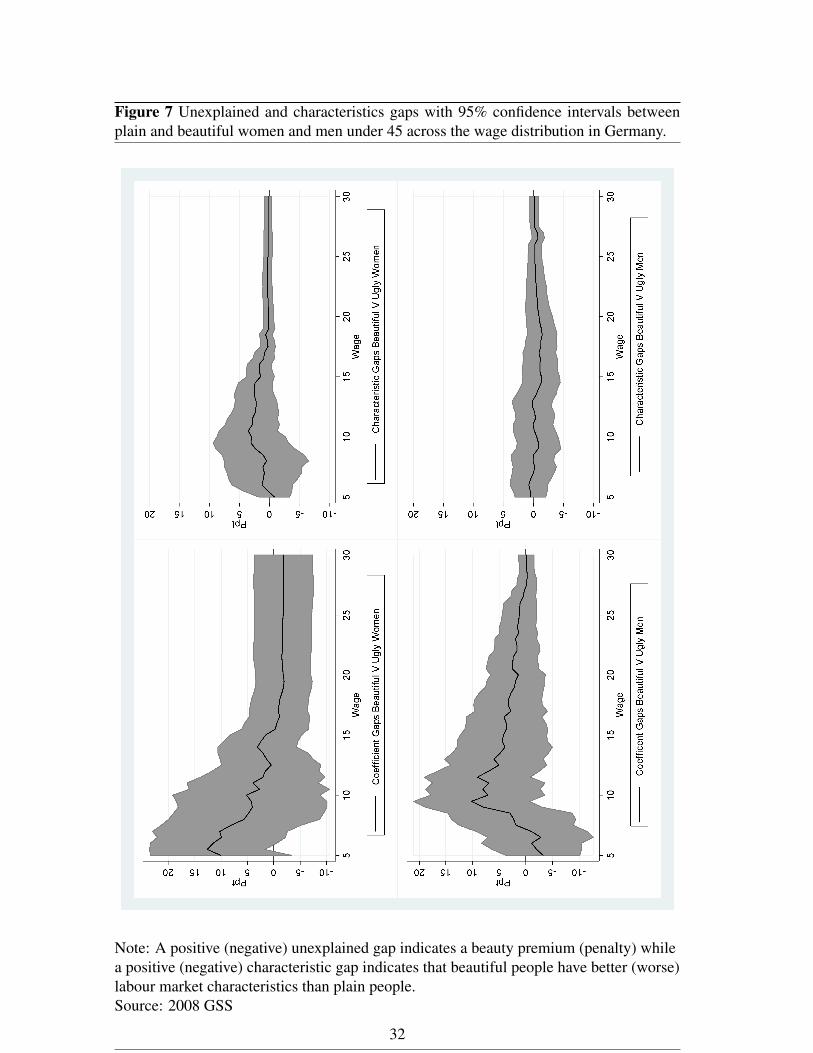
Figure 7 Unexplained and characteristics gaps with 95% confidence intervals betweenplain and beautiful women and men under 45 across the wage distribution in Germany.

Note: A positive (negative) unexplained gap indicates a beauty premium (penalty) whilea positive (negative) characteristic gap indicates that beautiful people have better (worse)labour market characteristics than plain people.Source: 2008 GSS

32

Figure A1 Self-assessed beauty by occupation (in percentages).

Source: 2007 PSELL3

33

Table A1: Select statistics for women and men in Luxembourg.

Women Men diffAge 37.325 38.104 -0.779∗∗

married 0.551 0.611 -0.060∗∗∗

single 0.311 0.307 0.004separated 0.138 0.082 0.056∗∗∗

no. children 1.226 1.283 -0.057children (0/1) 0.653 0.643 0.010lt high school 0.335 0.356 -0.020high school 0.305 0.328 -0.023college 0.348 0.310 0.038∗∗

Work experience 15.304 18.522 -3.218∗∗∗

full-time 0.686 0.979 -0.293∗∗∗

part-time 0.369 0.036 0.334∗∗∗

big company 0.454 0.556 -0.103∗∗∗

temporary contract 0.107 0.099 0.008civil servant 0.222 0.181 0.042∗∗∗

Native 0.387 0.367 0.020Portugese 0.239 0.282 -0.043∗∗∗

Other non-native 0.374 0.351 0.023bad health 0.035 0.025 0.010∗

great health 0.378 0.393 -0.015Occupation Type: Dressy 0.749 0.579 0.170∗∗∗

2007 PSELL-3; t statistics in parentheses * p<0.1 ** p<0.05 *** p<0.01

34

Table A2: Select statistics for women and men in Germany.

Women Men diffage 43.185 43.678 -0.493married 0.591 0.577 0.014single 0.240 0.322 -0.082∗∗∗

separated 0.167 0.101 0.066∗∗∗

no. children 0.675 0.533 0.141∗∗∗

children (0/1) 0.389 0.306 0.084∗∗∗

low education 0.243 0.240 0.002medium education 0.386 0.381 0.005high education 0.371 0.378 -0.007full-time 0.308 0.669 -0.360∗∗∗

part-time 0.584 0.290 0.294∗∗∗

big company 0.204 0.310 -0.106∗∗∗

civil servant 0.158 0.132 0.026∗

bad health 0.125 0.117 0.008great health 0.646 0.670 -0.024old fashioned 0.516 0.628 -0.111∗∗∗

working spouse 0.461 0.365 0.096∗∗∗

occupation type: dressy 0.761 0.453 0.308∗∗∗

Source: 2008 GSS; t statistics in parentheses * p<0.1 ** p<0.05 *** p<0.01

35