
MW NW Design PtP Technical Guidline
88
Ericssonwide Internal GUIDELINES 1 (88) Prepared (also subject responsible if other) No. KI/EAB/Z/NH Tyrone Vieira 1/102 60-FAY 111 08 Uen Approved Checked Date Rev Reference EAB/GD/S Mathias Edberg 2005-01-25 B Receiver KI/EAB/GD/S Mathias Edberg Microwave Network Design Part 1: Point-to-Point (PP) Microwave Planning Abstract This document provides together with Part 2: Point-to-multipoint (PMP) Microwave Planning basic and necessary guidelines for planning microwave networks. Both documents focus on the applicability of MINI-LINK equipment currently employed to connect radio base stations to RNC/MSC/BSC in the access portion of mobile networks. The guidelines in both documents attempt to provide the reader with basic and specific planning advices without entering into microwave theoretical aspects. In addition, the application of planning advices is vastly illustrated with practical examples performed in TEMS LinkPlanner. 1 Introduction.......................................................................................... 3 2 Microwave networks ............................................................................ 3 2.1 TEMS LinkPlanner application ............................................................ 5 3 MINI-LINK equipment .......................................................................... 6 3.1 Microwave networks ............................................................................ 6 3.2 MINI-LINK equipment .......................................................................... 6 3.3 Planning advices ............................................................................... 11 3.4 Redundancy ...................................................................................... 11 3.5 Radio frequencies ............................................................................. 12 3.6 Output power ranges and threshold levels ........................................ 13 3.7 Antenna data ..................................................................................... 13 3.8 Interference tolerance ....................................................................... 14 3.9 TEMS LinkPlanner application .......................................................... 14 4 Network configurations ...................................................................... 15 4.1 Chain/tandem/tree ............................................................................. 15 4.2 Star network Case A ...................................................................... 16 4.3 Star network Case B ...................................................................... 17 4.4 Ring (loop) ......................................................................................... 17 4.5 Mesh.................................................................................................. 18 4.6 Clusters ............................................................................................. 19 4.7 Radio-relay (microwave) environment ............................................... 19 4.8 Access and backbone in a ring ......................................................... 20 4.9 Planning advices ............................................................................... 20 5 The prediction cycle .......................................................................... 21 6 The loss/attenuation block................................................................. 21 6.1 Free-space loss ................................................................................. 22 6.2 Vegetation Attenuation ...................................................................... 23 6.3 Gas attenuation ................................................................................. 24
description
Ericsson MW NW design
Transcript of MW NW Design PtP Technical Guidline
Ericssonwide Internal
GUIDELINES 1 (88)Prepared (also subject responsible if other) No.
KI/EAB/Z/NH Tyrone Vieira 1/102 60-FAY 111 08 Uen Approved Checked Date Rev Reference
EAB/GD/S Mathias Edberg 2005-01-25 B
Receiver KI/EAB/GD/S Mathias Edberg
Microwave Network Design
Part 1: Point-to-Point (PP) Microwave Planning
Abstract
This document provides together with Part 2: Point-to-multipoint (PMP) Microwave Planning basic and necessary guidelines for planning microwave networks. Both documents focus on the applicability of MINI-LINK equipment currently employed to connect radio base stations to RNC/MSC/BSC in the access portion of mobile networks. The guidelines in both documents attempt to provide the reader with basic and specific planning advices without entering into microwave theoretical aspects. In addition, the application of planning advices is vastly illustrated with practical examples performed in TEMS LinkPlanner.
1 Introduction..........................................................................................3 2 Microwave networks............................................................................3 2.1 TEMS LinkPlanner application ............................................................5 3 MINI-LINK equipment..........................................................................6 3.1 Microwave networks............................................................................6 3.2 MINI-LINK equipment..........................................................................6 3.3 Planning advices ...............................................................................11 3.4 Redundancy ......................................................................................11 3.5 Radio frequencies .............................................................................12 3.6 Output power ranges and threshold levels........................................13 3.7 Antenna data .....................................................................................13 3.8 Interference tolerance .......................................................................14 3.9 TEMS LinkPlanner application ..........................................................14 4 Network configurations......................................................................15 4.1 Chain/tandem/tree.............................................................................15 4.2 Star network � Case A ......................................................................16 4.3 Star network � Case B ......................................................................17 4.4 Ring (loop).........................................................................................17 4.5 Mesh..................................................................................................18 4.6 Clusters .............................................................................................19 4.7 Radio-relay (microwave) environment...............................................19 4.8 Access and backbone in a ring .........................................................20 4.9 Planning advices ...............................................................................20 5 The prediction cycle ..........................................................................21 6 The loss/attenuation block.................................................................21 6.1 Free-space loss.................................................................................22 6.2 Vegetation Attenuation ......................................................................23 6.3 Gas attenuation .................................................................................24
Ericssonwide Internal
GUIDELINES 2 (88)Prepared (also subject responsible if other) No.
KI/EAB/Z/NH Tyrone Vieira 1/102 60-FAY 111 08 Uen Approved Checked Date Rev Reference
EAB/GD/S Mathias Edberg 2005-01-25 B
6.4 Attenuation due to precipitation.........................................................25 6.5 Attenuation due to obstacles .............................................................27 6.6 Attenuation due ground reflection .....................................................29 6.7 TEMS LinkPlanner application ..........................................................31 7 The fading block ................................................................................31 7.1 Multipath fading .................................................................................31 7.2 Rain fading ........................................................................................36 7.3 Refraction-Diffraction fading..............................................................36 7.4 Outage due to cross-polar discrimination..........................................37 7.5 The final fading picture ......................................................................38 7.6 TEMS Link Planner Application.........................................................38 8 The frequency planning/interference block .......................................39 8.1 Interference .......................................................................................39 8.2 Frequency planning of microwave networks .....................................43 8.3 Terminology for frequency planning ..................................................43 8.4 Channel arrangements......................................................................43 8.5 Channel width and spectral efficiency ...............................................46 8.6 Channel spacing for high capacity SDH links....................................46 8.7 Channel spacing for medium capacity SDH links..............................47 8.8 Network scenarios affecting frequency planning...............................47 8.9 Planning advices ...............................................................................49 8.10 Frequency planning: 10 crucial steps................................................50 8.11 Planning advices ...............................................................................51 8.12 TEMS LinkPlanner application ..........................................................53 9 The quality and availability block.......................................................53 9.1 Reference Q&A network model .........................................................54 9.2 Q&A Parameters ...............................................................................54 9.3 Allocation of Q&A objectives .............................................................55 9.4 Step-by-step procedure.....................................................................60 9.5 Planning advices ...............................................................................61 9.6 TEMS LinkPlanner application ..........................................................62 10 Planning procedures .........................................................................62 10.1 Design overview ................................................................................62 10.2 General remarks................................................................................63 10.3 Microwave path and chain.................................................................65 10.4 Map information.................................................................................65 10.5 Preliminary procedures .....................................................................66 10.6 Selecting radio-meteorological parameters .......................................69 10.7 Choosing allocation strategy .............................................................73 10.8 Application.........................................................................................73 11 References ........................................................................................88
Ericssonwide Internal
GUIDELINES 3 (88)Prepared (also subject responsible if other) No.
KI/EAB/Z/NH Tyrone Vieira 1/102 60-FAY 111 08 Uen Approved Checked Date Rev Reference
EAB/GD/S Mathias Edberg 2005-01-25 B
1 Introduction
Along with Part 2 (Point-to-Multipoint Microwave Planning), see [1], this guideline provides basic and advanced procedures for the design of microwave networks employing MINI-LINK. Both guidelines (Part 1: PP-Planning and Part 2: PMP-Planning) focus on the application of general microwave principles rather than theoretical issues.
The guideline starts with the presentation of current microwave networks (section 2), and then a summary of the basic issues of MINI-LINK equipment (section 3) required for carrying out a thorough microwave planning. Since radio stations are geographically established in accordance to several requirements, such as demographical aspects, capacity, terrain, infrastructures, etc, they might be connected following different configurations (section 4). The design of microwave links follows a prediction procedure (section 5) developed by Ericsson along the years. This procedure is known as the prediction cycle because of the iteration nature of the subject. The components of the prediction cycle (sections 6, 7, 8, and 9) are short and concise applications of the subjects of radiowave propagation, interference/frequency planning, and quality and availability allocation on microwave networks. From section 2 throughout section 9, a great number of Planning Advices are presented as hints and to facilitate the planning procedure. In order to emphasize planning issues, reference to a planning tool, TEMS LinkPlanner, is added at the end of each section, especially the sections forming the prediction cycle.
The structure of this Point-to-Point Microwave Guideline also reflects the conviction that full mastery of a subject of this nature cannot be accomplished without a significant amount of practice in using and applying the basic procedures that are developed in this guideline. Therefore, section 10 brings this guidelines to a close by illustrating the main parts of the planning procedure with a real, although limited microwave network composed of 20 sites employing TEMS LinkPlanner.
The readers that are familiar with basic microwave principles and planning procedures are strongly encouraged to move directly to section 10, and return to other sections whenever necessary.
2 Microwave networks
Current microwave networks are found in the transmission portions of WCDMA/GSM mobile networks, more specifically in the access portion where the traffic is transported between radio base stations and RNC/BSC. In addition to the access portion, there is a core portion that is extremely important for the vitality of the entire network. This part of the network requires a high degree of availability and is preferentially designed as rings connecting from a few sites up to tens of sites, where optical SDH and/or WDM dominates as the transmission medium.
Ericssonwide Internal
GUIDELINES 4 (88)Prepared (also subject responsible if other) No.
KI/EAB/Z/NH Tyrone Vieira 1/102 60-FAY 111 08 Uen Approved Checked Date Rev Reference
EAB/GD/S Mathias Edberg 2005-01-25 B
The access portion normally employs microwave links connecting a great number of sites and forming networks displaying different configurations. The core and the access portions of the network are structured in such a way that a Network Operation Center (NOC) handles issues as network performance, traffic management, and alarms.
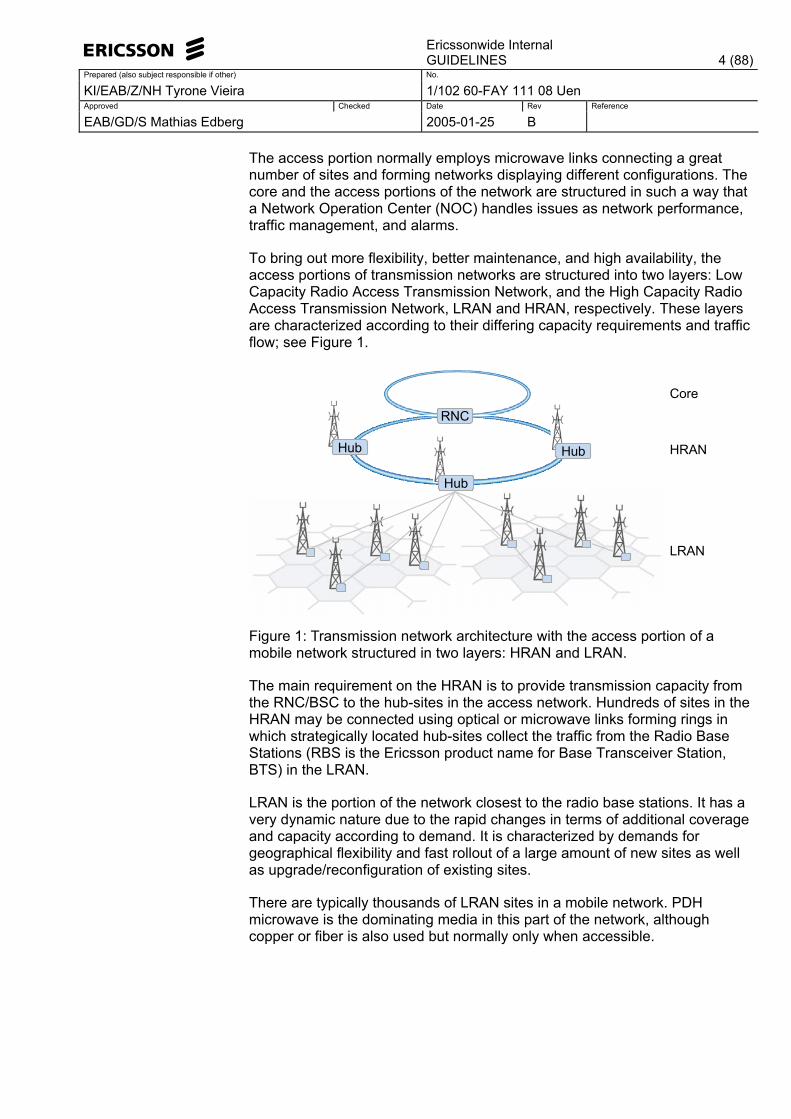
To bring out more flexibility, better maintenance, and high availability, the access portions of transmission networks are structured into two layers: Low Capacity Radio Access Transmission Network, and the High Capacity Radio Access Transmission Network, LRAN and HRAN, respectively. These layers are characterized according to their differing capacity requirements and traffic flow; see Figure 1.
Hub
HubHub
RNC
Core
HRAN
LRAN
Figure 1: Transmission network architecture with the access portion of a mobile network structured in two layers: HRAN and LRAN.
The main requirement on the HRAN is to provide transmission capacity from the RNC/BSC to the hub-sites in the access network. Hundreds of sites in the HRAN may be connected using optical or microwave links forming rings in which strategically located hub-sites collect the traffic from the Radio Base Stations (RBS is the Ericsson product name for Base Transceiver Station, BTS) in the LRAN.
LRAN is the portion of the network closest to the radio base stations. It has a very dynamic nature due to the rapid changes in terms of additional coverage and capacity according to demand. It is characterized by demands for geographical flexibility and fast rollout of a large amount of new sites as well as upgrade/reconfiguration of existing sites.
There are typically thousands of LRAN sites in a mobile network. PDH microwave is the dominating media in this part of the network, although copper or fiber is also used but normally only when accessible.
Ericssonwide Internal
GUIDELINES 5 (88)Prepared (also subject responsible if other) No.
KI/EAB/Z/NH Tyrone Vieira 1/102 60-FAY 111 08 Uen Approved Checked Date Rev Reference
EAB/GD/S Mathias Edberg 2005-01-25 B
Designers of Access Transport Networks are referred to [2] if support in choosing suitable solutions from the BTTN Product Portfolio is requested. This reference also provides information on how to select and specify the equipment needed for mobile networks.
2.1 TEMS LinkPlanner application
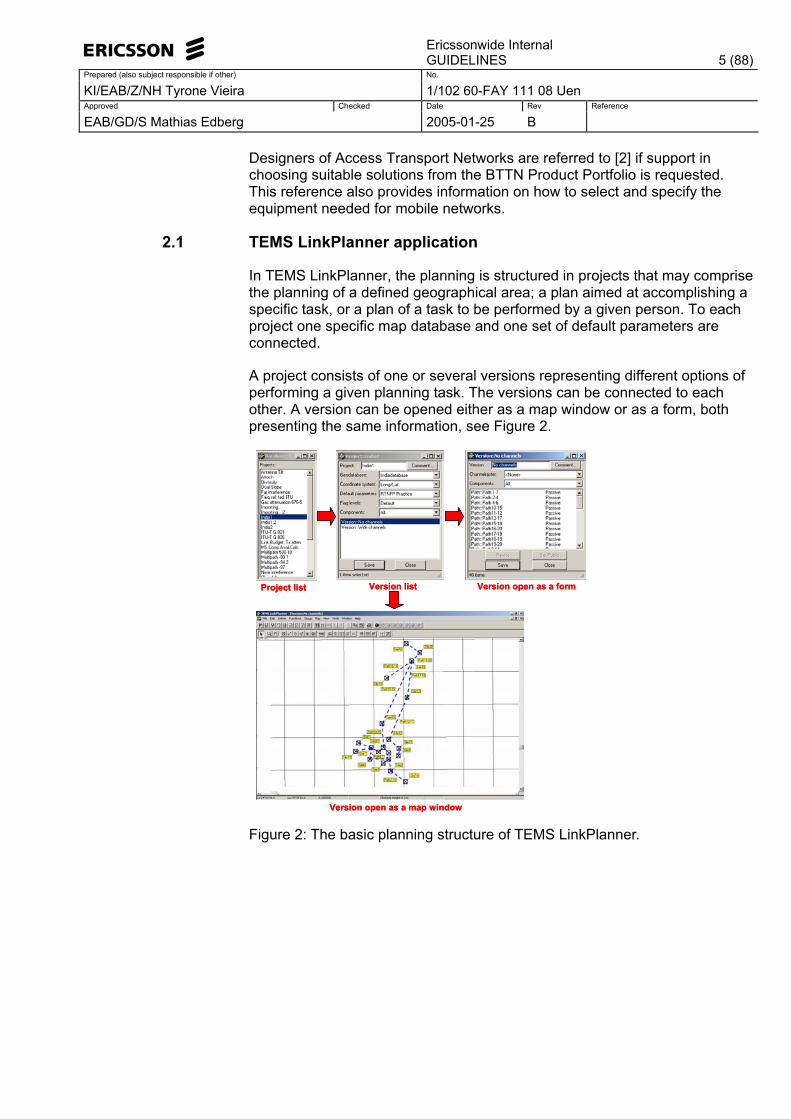
In TEMS LinkPlanner, the planning is structured in projects that may comprise the planning of a defined geographical area; a plan aimed at accomplishing a specific task, or a plan of a task to be performed by a given person. To each project one specific map database and one set of default parameters are connected.
A project consists of one or several versions representing different options of performing a given planning task. The versions can be connected to each other. A version can be opened either as a map window or as a form, both presenting the same information, see Figure 2.
Project list Version list Version open as a form
Version open as a map window
Project list Version list Version open as a form
Version open as a map window Figure 2: The basic planning structure of TEMS LinkPlanner.
Ericssonwide Internal
GUIDELINES 6 (88)Prepared (also subject responsible if other) No.
KI/EAB/Z/NH Tyrone Vieira 1/102 60-FAY 111 08 Uen Approved Checked Date Rev Reference
EAB/GD/S Mathias Edberg 2005-01-25 B
3 MINI-LINK equipment
3.1 Microwave networks
Microwave networks are attractive transmission alternatives for applications ranging from the coverage of rural, sparsely populated areas of developing countries having ineffective or minimal infrastructures to well-developed industrial countries that require rapid expansion of telecommunications networks. Most of the commercial radio links currently in use are in the frequency range 2�50 GHz.
3.2 MINI-LINK equipment
MINI-LINK radio-equipment is available for PDH and SDH traffic. For PDH traffic and depending on the capacity demands, there are two modulation methods: 16 QAM and C-QPSK. For SDH traffic two modulation methods are available: 16 QAM and 128 QAM. MINI-LINK PDH equipment, also known as �PDH links�, are currently called MINI-LINK E or �MINI-LINK E Medium Capacity�, while SDH equipment, also known as �SDH links�, are currently called MINI-LINK High Capacity. Both are also commonly referred to as �MINI-LINK terminals�.
Detailed information on MINI-LINK equipment parameters useful for network design is obtained in the following product specifications: • MINI-LINK E 16QAM: [3]. • MINI-LINK E C-QPSK: [4]. • MINI-LINK High Capacity: [5].
Complete and detailed information on application, installation, operation & maintenance of MINI-LINK equipment is obtained from the following libraries: • MINI-LINK E ETSI: [7]. • MINI-LINK E ANSI: [8]. • MINI-LINK High Capacity: [9].
3.2.1 MINI-LINK E Medium Capacity
3.2.1.1 System setup
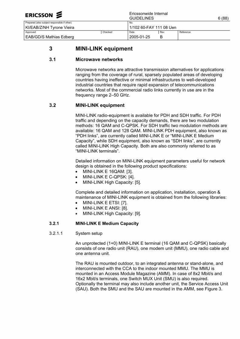
An unprotected (1+0) MINI-LINK E terminal (16 QAM and C-QPSK) basically consists of one radio unit (RAU), one modem unit (MMU), one radio cable and one antenna unit.
The RAU is mounted outdoor, to an integrated antenna or stand-alone, and interconnected with the CCA to the indoor mounted MMU. The MMU is mounted in an Access Module Magazine (AMM). In case of 8x2 Mbit/s and 16x2 Mbit/s terminals, one Switch MUX Unit (SMU) is also required. Optionally the terminal may also include another unit, the Service Access Unit (SAU). Both the SMU and the SAU are mounted in the AMM, see Figure 3.
Ericssonwide Internal
GUIDELINES 7 (88)Prepared (also subject responsible if other) No.
KI/EAB/Z/NH Tyrone Vieira 1/102 60-FAY 111 08 Uen Approved Checked Date Rev Reference
EAB/GD/S Mathias Edberg 2005-01-25 B
MMUSMU/SWU RAUCCA
AMM
Figure 3:Unprotected (1+0) MINI-LINK E terminal. One Switch MUX Unit (SMU) is also required if 8x2 Mbit/s and 16x2 Mbit/s terminals are required.
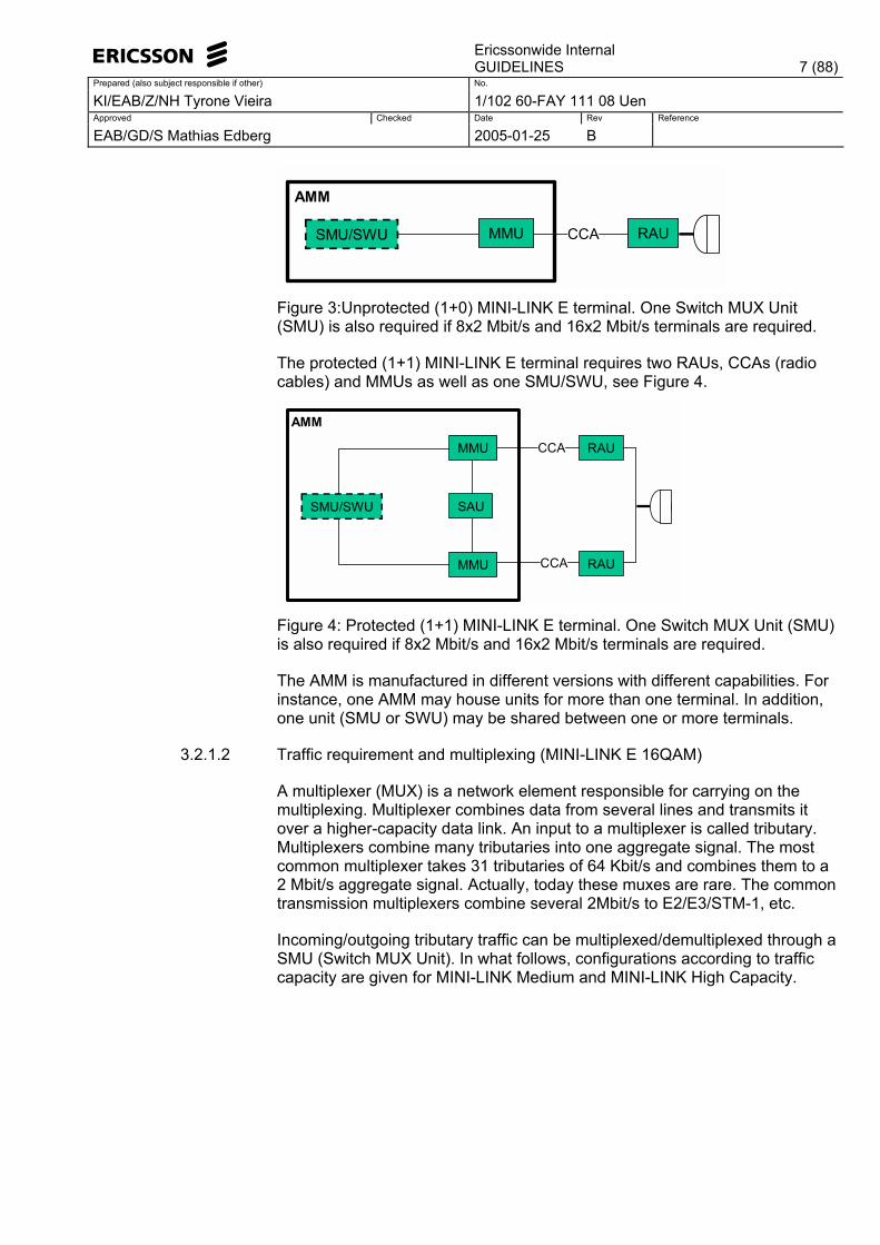
The protected (1+1) MINI-LINK E terminal requires two RAUs, CCAs (radio cables) and MMUs as well as one SMU/SWU, see Figure 4.
MMU
MMU
SAUSMU/SWU
RAU
RAU
AMM
CCA
CCA
Figure 4: Protected (1+1) MINI-LINK E terminal. One Switch MUX Unit (SMU) is also required if 8x2 Mbit/s and 16x2 Mbit/s terminals are required.
The AMM is manufactured in different versions with different capabilities. For instance, one AMM may house units for more than one terminal. In addition, one unit (SMU or SWU) may be shared between one or more terminals.
3.2.1.2 Traffic requirement and multiplexing (MINI-LINK E 16QAM)
A multiplexer (MUX) is a network element responsible for carrying on the multiplexing. Multiplexer combines data from several lines and transmits it over a higher-capacity data link. An input to a multiplexer is called tributary. Multiplexers combine many tributaries into one aggregate signal. The most common multiplexer takes 31 tributaries of 64 Kbit/s and combines them to a 2 Mbit/s aggregate signal. Actually, today these muxes are rare. The common transmission multiplexers combine several 2Mbit/s to E2/E3/STM-1, etc.
Incoming/outgoing tributary traffic can be multiplexed/demultiplexed through a SMU (Switch MUX Unit). In what follows, configurations according to traffic capacity are given for MINI-LINK Medium and MINI-LINK High Capacity.
Ericssonwide Internal
GUIDELINES 8 (88)Prepared (also subject responsible if other) No.
KI/EAB/Z/NH Tyrone Vieira 1/102 60-FAY 111 08 Uen Approved Checked Date Rev Reference
EAB/GD/S Mathias Edberg 2005-01-25 B
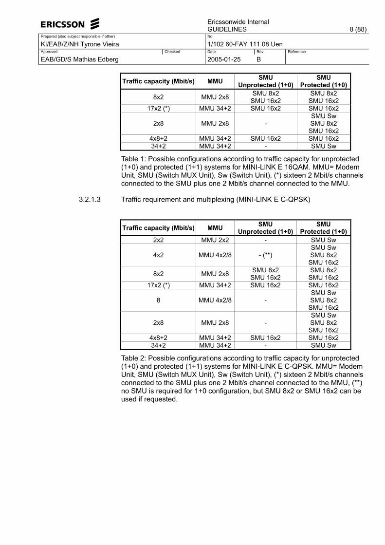
Traffic capacity (Mbit/s) MMU SMU Unprotected (1+0)
SMU Protected (1+0)
8x2 MMU 2x8 SMU 8x2 SMU 16x2
SMU 8x2 SMU 16x2
17x2 (*) MMU 34+2 SMU 16x2 SMU 16x2
2x8 MMU 2x8 - SMU Sw SMU 8x2 SMU 16x2
4x8+2 MMU 34+2 SMU 16x2 SMU 16x2 34+2 MMU 34+2 - SMU Sw
Table 1: Possible configurations according to traffic capacity for unprotected (1+0) and protected (1+1) systems for MINI-LINK E 16QAM. MMU= Modem Unit, SMU (Switch MUX Unit), Sw (Switch Unit), (*) sixteen 2 Mbit/s channels connected to the SMU plus one 2 Mbit/s channel connected to the MMU.
3.2.1.3 Traffic requirement and multiplexing (MINI-LINK E C-QPSK)
Traffic capacity (Mbit/s) MMU SMU Unprotected (1+0)
SMU Protected (1+0)
2x2 MMU 2x2 - SMU Sw
4x2 MMU 4x2/8 - (**) SMU Sw SMU 8x2
SMU 16x2
8x2 MMU 2x8 SMU 8x2 SMU 16x2
SMU 8x2 SMU 16x2
17x2 (*) MMU 34+2 SMU 16x2 SMU 16x2
8 MMU 4x2/8 - SMU Sw SMU 8x2
SMU 16x2
2x8 MMU 2x8 - SMU Sw SMU 8x2
SMU 16x2 4x8+2 MMU 34+2 SMU 16x2 SMU 16x2 34+2 MMU 34+2 - SMU Sw
Table 2: Possible configurations according to traffic capacity for unprotected (1+0) and protected (1+1) systems for MINI-LINK E C-QPSK. MMU= Modem Unit, SMU (Switch MUX Unit), Sw (Switch Unit), (*) sixteen 2 Mbit/s channels connected to the SMU plus one 2 Mbit/s channel connected to the MMU, (**) no SMU is required for 1+0 configuration, but SMU 8x2 or SMU 16x2 can be used if requested.
Ericssonwide Internal
GUIDELINES 9 (88)Prepared (also subject responsible if other) No.
KI/EAB/Z/NH Tyrone Vieira 1/102 60-FAY 111 08 Uen Approved Checked Date Rev Reference
EAB/GD/S Mathias Edberg 2005-01-25 B
3.2.2 MINI-LINK High Capacity
3.2.2.1 System setup
An unprotected (1+0) MINI-LINK High Capacity terminal consists basically of one radio unit (RAU), one modem unit (MMU), and one radio cable. In addition, there is one more unit, the Traffic and Service Unit (TRU) with the principal function of terminating/generating a standardized STM-1/STS-3 signal, and transmit/receive it to/from the MMU. The system setups are similar to the MINI-LINK E terminal presented in the previous section for both unprotected and protected features.
This AMM unit provides housing for the TRU and MMU as well as cooling and power distribution. The AMM is manufactured in two different features: AMM 1U-1: 1U High having the capability to house two units and AMM 2U-4: 2U High, having the capability to house four units.
As mentioned before, the MMU is available in two different features:
MMU 155/16. By using 16QAM modulation, it is possible to fit 50/55/56/80 MHz of bandwidth.
MMU 155/128. By using 128QAM modulation, it is possible to fit 27.5/28/40/50 MHz of bandwidth.
Unprotected terminal (1+0) can be based either on the AMM 1U-1 or AMM 2U-4. The AMM 2U-4 allows the equipment to be upgraded either to 1+1 or 2x(1+0) configuration without changing the access module magazine.
In terminal configuration 2x(1+0), both receivers and transmitters are working and two different signals are transmitted with two different frequencies.
3.2.2.2 Traffic requirement and multiplexing
The channel capacity provided by an STM-1 has been designed to provide transport for a 140 Mbit/s tributary signal. At the same time different PDH frames can be transported using the STM-N frame. To have some kind of structure, the STM-N payload has been divided in smaller parts called Tributary Units (TUs), or Administrative Units (AUs), which have a fixed position in the frame.
The PDH traffic is �packed� inside Virtual Containers (VCs). This operation is called mapping. The size of the VC is according to the capacity of the PDH frame inside. These VCs, after being assembled in the TTP, are placed inside TUs or AUs, which size is corresponding to the VC size. Then, there are TU-11 (which can carry one VC-11), TU-12 (the same with VC-12), TU-2 (VC-2), TU-3 (for lower order VC-3), AU-3 (for higher order VC-3), and AU-4 (VC-4). Inserting a VC inside a TU/AU is called aligning.
Ericssonwide Internal
GUIDELINES 10 (88)Prepared (also subject responsible if other) No.
KI/EAB/Z/NH Tyrone Vieira 1/102 60-FAY 111 08 Uen Approved Checked Date Rev Reference
EAB/GD/S Mathias Edberg 2005-01-25 B
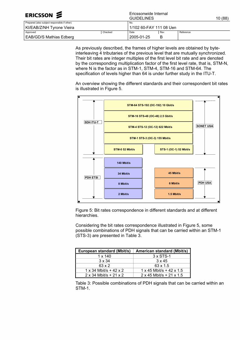
As previously described, the frames of higher levels are obtained by byte-interleaving 4 tributaries of the previous level that are mutually synchronized. Their bit rates are integer multiples of the first level bit rate and are denoted by the corresponding multiplication factor of the first level rate, that is, STM-N, where N is the factor as in STM-1, STM-4, STM-16 and STM-64. The specification of levels higher than 64 is under further study in the ITU-T.
An overview showing the different standards and their correspondent bit rates is illustrated in Figure 5.
2 Mbit/s
140 Mbit/s
34 Mbit/s
8 Mbit/s
1.5 Mbit/s
6 Mbit/s
45 Mbit/s
STS-1 (OC-1) 52 Mbit/s
STM-1 STS-3 (OC-3) 155 Mbit/s
STM-64 STS-192 (OC-192) 10 Gbit/s
STM-16 STS-48 (OC-48) 2.5 Gbit/s
STM-4 STS-12 (OC-12) 622 Mbit/s
PDH ETSI PDH USA
SONET USASDH ITU-T
STM-0 52 Mbit/s
Figure 5: Bit rates correspondence in different standards and at different hierarchies.
Considering the bit rates correspondence illustrated in Figure 5, some possible combinations of PDH signals that can be carried within an STM-1 (STS-3) are presented in Table 3.
European standard (Mbit/s) American standard (Mbit/s)
1 x 140 3 x STS-1 3 x 34 3 x 45 63 x 2 63 x 1.5
1 x 34 Mbit/s + 42 x 2 1 x 45 Mbit/s + 42 x 1.5 2 x 34 Mbit/s + 21 x 2 2 x 45 Mbit/s + 21 x 1.5
Table 3: Possible combinations of PDH signals that can be carried within an STM-1.
Ericssonwide Internal
GUIDELINES 11 (88)Prepared (also subject responsible if other) No.
KI/EAB/Z/NH Tyrone Vieira 1/102 60-FAY 111 08 Uen Approved Checked Date Rev Reference
EAB/GD/S Mathias Edberg 2005-01-25 B
3.3 Planning advices • RAU L High Capacity Radio Unit provides 155 Mbit/s capacity using 16
QAM and 128 QAM modulations. The letter L in the end of the product name indicates high capacity radios.
• RAU N Agile Radio Unit provides 2x2 up to 155 Mbit/s using C-QPSK, 16 QAM and 128 QAM modulations. The letter N in the end of the product name indicates agile radios.
3.4 Redundancy
In Hot Standby mode, one transmitter is working while the other one is in Standby, not transmitting but ready to transmit if the active one fails. Both radio units are receiving signals. To manage difficult propagation conditions, 1+1 configuration can also be provided in either frequency diversity or space diversity solution.
3.4.1 Hardware failure
Hardware failure lasts normally longer than 10 consecutive seconds and therefore gives UATR. In fact, the UATR objectives given by the ITU-R shall account for unavailability due to radiowave propagation and hardware failure.
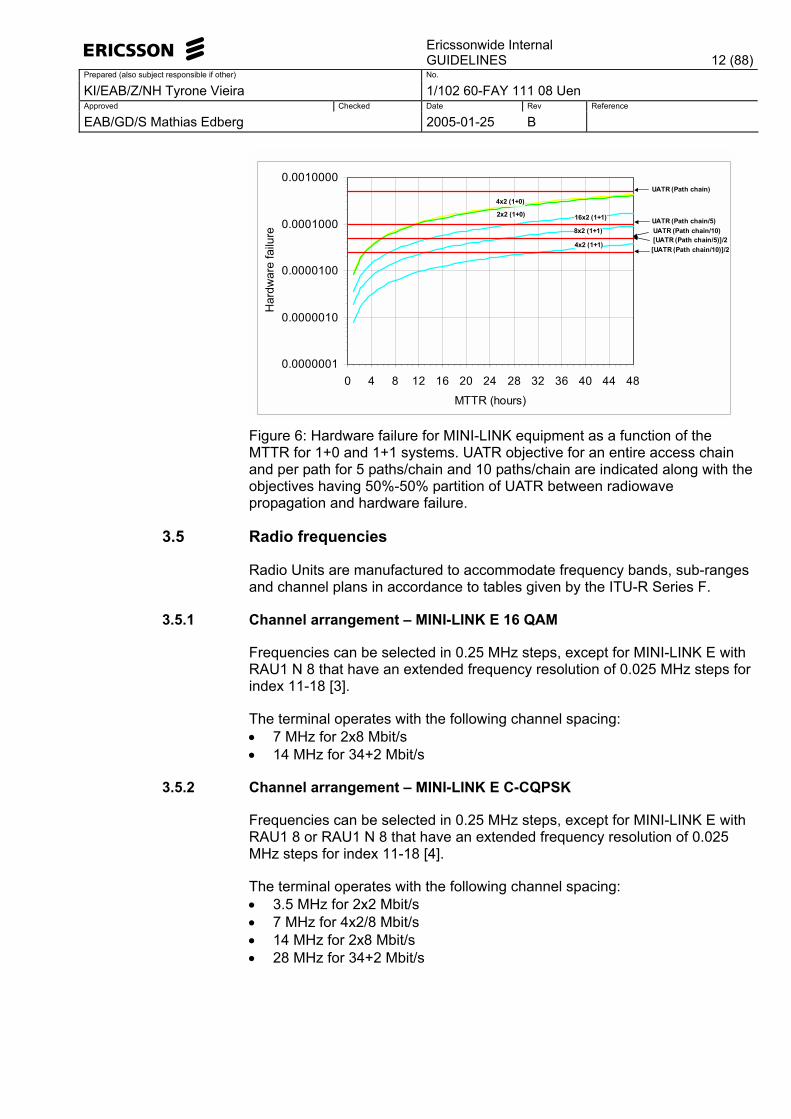
Figure 6 illustrates the contribution given by hardware failure for MINI-LINK equipment for the system setups illustrated in Figure 4 and Figure 5 for unprotected and protected, respectively. The hardware failure is given as a function of the required MTTR for 2x2 and 4x2 (1+0) and 4x2, 8x2 and 16x2 (1+1). The UATR objective 0.0005 is for one entire access chain and given in Rec. ITU-R F.1493 (based on Rec. ITU-T G.827). It is used for MINI-LINK Medium Capacity (16QAM and C-QPSK) and MINI-LINK High Capacity (16QAM and 128QAM). The objectives are per path, where 0.0001 is for 5 paths/chain and 0.00005 is for 10 paths/chain. The partition between UATR due to radiowave propagation and hardware failure is 50%-50% of 0.0001 and 0.00005, which is indicated in Figure 6 as [UATR (path chain/5]/2 and [UATR (path chain/10]/2, respectively.
Figure 6 shows clearly that if 10 paths/chain is considered, then only protected setups can have MTTR-values longer than 4 hours, irrespectively of the capacity (higher capacity gives short MTTR if the same objective is fulfilled). However, if 5 paths/chain is considered, then both protected and unprotected system can have MTTR-values longer than 4 hours, irrespectively of the capacity.
Ericssonwide Internal
GUIDELINES 12 (88)Prepared (also subject responsible if other) No.
KI/EAB/Z/NH Tyrone Vieira 1/102 60-FAY 111 08 Uen Approved Checked Date Rev Reference
EAB/GD/S Mathias Edberg 2005-01-25 B
0.0000001
0.0000010
0.0000100
0.0001000
0.0010000
0 4 8 12 16 20 24 28 32 36 40 44 48
MTTR (hours)
Har
dwar
e fa
ilure
UATR (Path chain)
UATR (Path chain/5)UATR (Path chain/10)[UATR (Path chain/5)]/2
4x2 (1+1)
8x2 (1+1)
16x2 (1+1)2x2 (1+0)
4x2 (1+0)
[UATR (Path chain/10)]/2
Figure 6: Hardware failure for MINI-LINK equipment as a function of the MTTR for 1+0 and 1+1 systems. UATR objective for an entire access chain and per path for 5 paths/chain and 10 paths/chain are indicated along with the objectives having 50%-50% partition of UATR between radiowave propagation and hardware failure.
3.5 Radio frequencies
Radio Units are manufactured to accommodate frequency bands, sub-ranges and channel plans in accordance to tables given by the ITU-R Series F.
3.5.1 Channel arrangement � MINI-LINK E 16 QAM
Frequencies can be selected in 0.25 MHz steps, except for MINI-LINK E with RAU1 N 8 that have an extended frequency resolution of 0.025 MHz steps for index 11-18 [3].
The terminal operates with the following channel spacing: • 7 MHz for 2x8 Mbit/s • 14 MHz for 34+2 Mbit/s
3.5.2 Channel arrangement � MINI-LINK E C-CQPSK
Frequencies can be selected in 0.25 MHz steps, except for MINI-LINK E with RAU1 8 or RAU1 N 8 that have an extended frequency resolution of 0.025 MHz steps for index 11-18 [4].
The terminal operates with the following channel spacing: • 3.5 MHz for 2x2 Mbit/s • 7 MHz for 4x2/8 Mbit/s • 14 MHz for 2x8 Mbit/s • 28 MHz for 34+2 Mbit/s
Ericssonwide Internal
GUIDELINES 13 (88)Prepared (also subject responsible if other) No.
KI/EAB/Z/NH Tyrone Vieira 1/102 60-FAY 111 08 Uen Approved Checked Date Rev Reference
EAB/GD/S Mathias Edberg 2005-01-25 B
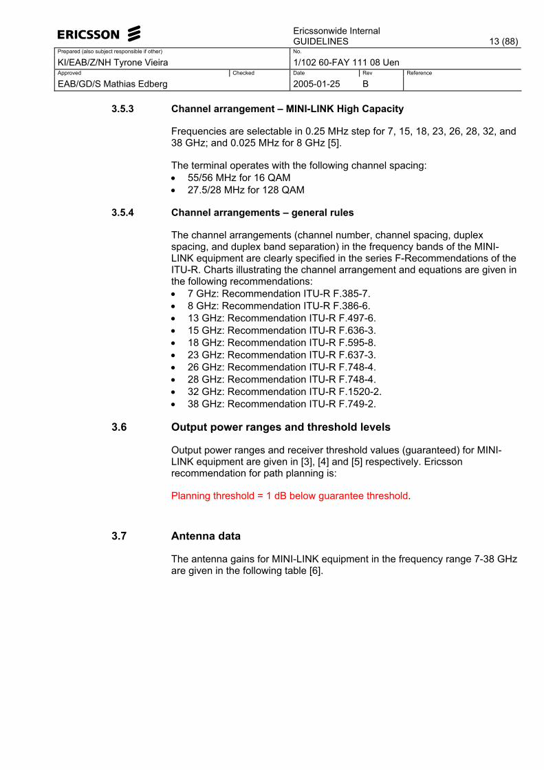
3.5.3 Channel arrangement � MINI-LINK High Capacity
Frequencies are selectable in 0.25 MHz step for 7, 15, 18, 23, 26, 28, 32, and 38 GHz; and 0.025 MHz for 8 GHz [5].
The terminal operates with the following channel spacing: • 55/56 MHz for 16 QAM • 27.5/28 MHz for 128 QAM
3.5.4 Channel arrangements � general rules
The channel arrangements (channel number, channel spacing, duplex spacing, and duplex band separation) in the frequency bands of the MINI-LINK equipment are clearly specified in the series F-Recommendations of the ITU-R. Charts illustrating the channel arrangement and equations are given in the following recommendations: • 7 GHz: Recommendation ITU-R F.385-7. • 8 GHz: Recommendation ITU-R F.386-6. • 13 GHz: Recommendation ITU-R F.497-6. • 15 GHz: Recommendation ITU-R F.636-3. • 18 GHz: Recommendation ITU-R F.595-8. • 23 GHz: Recommendation ITU-R F.637-3. • 26 GHz: Recommendation ITU-R F.748-4. • 28 GHz: Recommendation ITU-R F.748-4. • 32 GHz: Recommendation ITU-R F.1520-2. • 38 GHz: Recommendation ITU-R F.749-2.
3.6 Output power ranges and threshold levels
Output power ranges and receiver threshold values (guaranteed) for MINI-LINK equipment are given in [3], [4] and [5] respectively. Ericsson recommendation for path planning is:
Planning threshold = 1 dB below guarantee threshold.
3.7 Antenna data
The antenna gains for MINI-LINK equipment in the frequency range 7-38 GHz are given in the following table [6].
Ericssonwide Internal
GUIDELINES 14 (88)Prepared (also subject responsible if other) No.
KI/EAB/Z/NH Tyrone Vieira 1/102 60-FAY 111 08 Uen Approved Checked Date Rev Reference
EAB/GD/S Mathias Edberg 2005-01-25 B
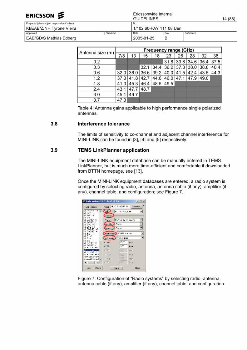
Frequency range (GHz) Antenna size (m)7/8 13 15 18 23 26 28 32 38
0.2 31.8 33.8 34.6 35.4 37.50.3 32.1 34.4 36.2 37.3 38.0 38.8 40.40.6 32.0 36.0 36.6 39.2 40.0 41.5 42.4 43.5 44.31.2 37.0 41.8 42.7 44.6 46.0 47.1 47.9 49.0 1.8 41.0 45.3 46.4 48.5 49.5 2.4 43.1 47.7 48.7 3.0 45.1 49.7 3.7 47.3
Table 4: Antenna gains applicable to high performance single polarized antennas.
3.8 Interference tolerance
The limits of sensitivity to co-channel and adjacent channel interference for MINI-LINK can be found in [3], [4] and [5] respectively.
3.9 TEMS LinkPlanner application
The MINI-LINK equipment database can be manually entered in TEMS LinkPlanner, but is much more time-efficient and comfortable if downloaded from BTTN homepage, see [13].
Once the MINI-LINK equipment databases are entered, a radio system is configured by selecting radio, antenna, antenna cable (if any), amplifier (if any), channel table, and configuration; see Figure 7.
Figure 7: Configuration of �Radio systems� by selecting radio, antenna, antenna cable (if any), amplifier (if any), channel table, and configuration.
Ericssonwide Internal
GUIDELINES 15 (88)Prepared (also subject responsible if other) No.
KI/EAB/Z/NH Tyrone Vieira 1/102 60-FAY 111 08 Uen Approved Checked Date Rev Reference
EAB/GD/S Mathias Edberg 2005-01-25 B
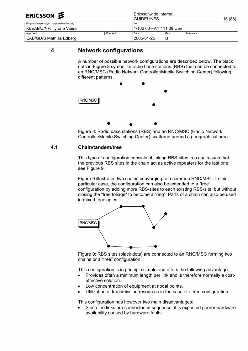
4 Network configurations
A number of possible network configurations are described below. The black dots in Figure 8 symbolize radio base stations (RBS) that can be connected to an RNC/MSC (Radio Network Controller/Mobile Switching Center) following different patterns.
RNC/MSC
Figure 8: Radio base stations (RBS) and an RNC/MSC (Radio Network Controller/Mobile Switching Center) scattered around a geographical area.
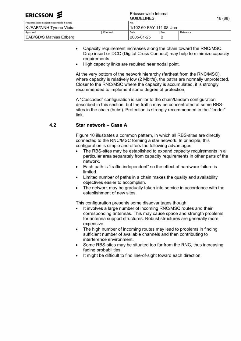
4.1 Chain/tandem/tree
This type of configuration consists of linking RBS-sites in a chain such that the previous RBS sites in the chain act as active repeaters for the last one; see Figure 9.
Figure 9 illustrates two chains converging to a common RNC/MSC. In this particular case, the configuration can also be extended to a �tree� configuration by adding more RBS-sites to each existing RBS-site, but without closing the �tree foliage� to become a �ring�. Parts of a chain can also be used in mixed topologies.
RNC/MSC
Figure 9: RBS sites (black dots) are connected to an RNC/MSC forming two chains or a �tree� configuration.
This configuration is in principle simple and offers the following advantage: • Provides often a minimum length per link and is therefore normally a cost-
effective solution. • Low concentration of equipment at nodal points. • Utilization of transmission resources in the case of a tree configuration.
This configuration has however two main disadvantages: • Since the links are connected in sequence, it is expected poorer hardware
availability caused by hardware faults.
Ericssonwide Internal
GUIDELINES 16 (88)Prepared (also subject responsible if other) No.
KI/EAB/Z/NH Tyrone Vieira 1/102 60-FAY 111 08 Uen Approved Checked Date Rev Reference
EAB/GD/S Mathias Edberg 2005-01-25 B
• Capacity requirement increases along the chain toward the RNC/MSC. Drop insert or DCC (Digital Cross Connect) may help to minimize capacity requirements.
• High capacity links are required near nodal point.
At the very bottom of the network hierarchy (farthest from the RNC/MSC), where capacity is relatively low (2 Mbit/s), the paths are normally unprotected. Closer to the RNC/MSC where the capacity is accumulated, it is strongly recommended to implement some degree of protection.
A �Cascaded� configuration is similar to the chain/tandem configuration described in this section, but the traffic may be concentrated at some RBS-sites in the chain (hubs). Protection is strongly recommended in the �feeder� link.
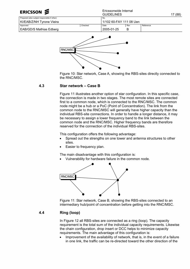
4.2 Star network � Case A
Figure 10 illustrates a common pattern, in which all RBS-sites are directly connected to the RNC/MSC forming a star network. In principle, this configuration is simple and offers the following advantages: • The RBS-sites may be established to expand capacity requirements in a
particular area separately from capacity requirements in other parts of the network.
• Each path is �traffic-independent� so the effect of hardware failure is limited.
• Limited number of paths in a chain makes the quality and availability objectives easier to accomplish.
• The network may be gradually taken into service in accordance with the establishment of new sites.
This configuration presents some disadvantages though: • It involves a large number of incoming RNC/MSC routes and their
corresponding antennas. This may cause space and strength problems for antenna support structures. Robust structures are generally more expensive.
• The high number of incoming routes may lead to problems in finding sufficient number of available channels and then contributing to interference environment.
• Some RBS-sites may be situated too far from the RNC, thus increasing fading probabilities.
• It might be difficult to find line-of-sight toward each direction.
Ericssonwide Internal
GUIDELINES 17 (88)Prepared (also subject responsible if other) No.
KI/EAB/Z/NH Tyrone Vieira 1/102 60-FAY 111 08 Uen Approved Checked Date Rev Reference
EAB/GD/S Mathias Edberg 2005-01-25 B
RNC/MSC
Figure 10: Star network, Case A, showing the RBS-sites directly connected to the RNC/MSC.
4.3 Star network � Case B
Figure 11 illustrates another option of star configuration. In this specific case, the connection is made in two stages. The most remote sites are connected first to a common node, which is connected to the RNC/MSC. The common node might be a hub or a PoC (Point of Concentration). The link from the common node to the RNC/MSC will generally have higher capacity than the individual RBS-site connections. In order to handle a longer distance, it may be necessary to assign a lower frequency band to the link between the common node and the RNC/MSC. Higher frequency bands are therefore reserved for the connection of the individual RBS-sites.
This configuration offers the following advantage: • Spread out the strengths on one tower and antenna structures to other
sites. • Easier to frequency plan.
The main disadvantage with this configuration is: • Vulnerability for hardware failure in the common node.
RNC/MSC
Figure 11: Star network, Case B, showing the RBS-sites connected to an intermediary hub/point of concentration before getting into the RNC/MSC.
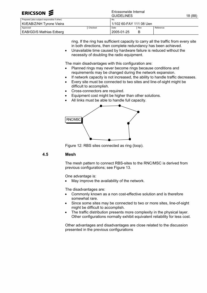
4.4 Ring (loop)
In Figure 12 all RBS-sites are connected as a ring (loop). The capacity requirement is the total sum of the individual capacity requirements. Likewise the chain configuration, drop insert or DCC helps to minimize capacity requirements. The main advantage of this configuration is: • Improvement of the availability of network, that is, in the event of a failure
in one link, the traffic can be re-directed toward the other direction of the
Ericssonwide Internal
GUIDELINES 18 (88)Prepared (also subject responsible if other) No.
KI/EAB/Z/NH Tyrone Vieira 1/102 60-FAY 111 08 Uen Approved Checked Date Rev Reference
EAB/GD/S Mathias Edberg 2005-01-25 B
ring. If the ring has sufficient capacity to carry all the traffic from every site in both directions, then complete redundancy has been achieved.
• Unavailable time caused by hardware failure is reduced without the necessity of doubling the radio equipment.
The main disadvantages with this configuration are: • Planned rings may never become rings because conditions and
requirements may be changed during the network expansion. • If network capacity is not increased, the ability to handle traffic decreases. • Every site must be connected to two sites and line-of-sight might be
difficult to accomplish. • Cross-connectors are required. • Equipment cost might be higher than other solutions. • All links must be able to handle full capacity.
RNC/MSC
Figure 12: RBS sites connected as ring (loop).
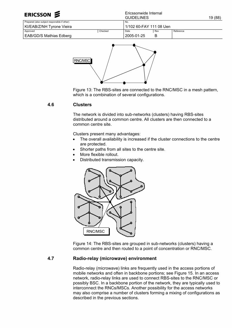
4.5 Mesh
The mesh pattern to connect RBS-sites to the RNC/MSC is derived from previous configurations; see Figure 13.
One advantage is: • May improve the availability of the network.
The disadvantages are: • Commonly known as a non cost-effective solution and is therefore
somewhat rare. • Since some sites may be connected to two or more sites, line-of-sight
might be difficult to accomplish. • The traffic distribution presents more complexity in the physical layer.
Other configurations normally exhibit equivalent reliability for less cost.
Other advantages and disadvantages are close related to the discussion presented in the previous configurations
Ericssonwide Internal
GUIDELINES 19 (88)Prepared (also subject responsible if other) No.
KI/EAB/Z/NH Tyrone Vieira 1/102 60-FAY 111 08 Uen Approved Checked Date Rev Reference
EAB/GD/S Mathias Edberg 2005-01-25 B
RNC/MSC
Figure 13: The RBS-sites are connected to the RNC/MSC in a mesh pattern, which is a combination of several configurations.
4.6 Clusters
The network is divided into sub-networks (clusters) having RBS-sites distributed around a common centre. All clusters are then connected to a common centre site.
Clusters present many advantages: • The overall availability is increased if the cluster connections to the centre
are protected. • Shorter paths from all sites to the centre site. • More flexible rollout. • Distributed transmission capacity.
RNC/MSC
Figure 14: The RBS-sites are grouped in sub-networks (clusters) having a common centre and then routed to a point of concentration or RNC/MSC.
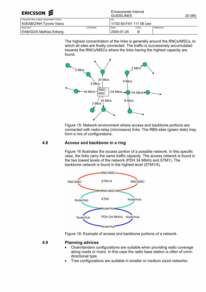
4.7 Radio-relay (microwave) environment
Radio-relay (microwave) links are frequently used in the access portions of mobile networks and often in backbone portions; see Figure 15. In an access network, radio-relay links are used to connect RBS-sites to the RNC/MSC or possibly BSC. In a backbone portion of the network, they are typically used to interconnect the RNCs/MSCs. Another possibility for the access networks may also comprise a number of clusters forming a mixing of configurations as described in the previous sections.
Ericssonwide Internal
GUIDELINES 20 (88)Prepared (also subject responsible if other) No.
KI/EAB/Z/NH Tyrone Vieira 1/102 60-FAY 111 08 Uen Approved Checked Date Rev Reference
EAB/GD/S Mathias Edberg 2005-01-25 B
The highest concentration of the links is generally around the RNCs/MSCs, to which all sites are finally connected. The traffic is successively accumulated towards the RNCs/MSCs where the links having the highest capacity are found.
34 Mb/s
34 Mb/s
34 Mb/s
34 Mb/s
34 Mb/s
8 Mb/s
2 Mb/s2 Mb/s
8 Mb/s
8 Mb/s2 Mb/s
RNC/ MSC
Figure 15: Network environment where access and backbone portions are connected with radio-relay (microwave) links. The RBS-sites (green dots) may form a mix of configurations.
4.8 Access and backbone in a ring
Figure 16 illustrates the access portion of a possible network. In this specific case, the links carry the same traffic capacity. The access network is found in the two lowest levels of the network (PDH 34 Mbit/s and STM1). The backbone network is found in the highest level (STM1/4).
RNC/MSC
RNC/MSC
RNC/MSC
RNC/MSCSTM1/4
Node/Hub Node/Hub
Node/Hub
STM1
PDH (34 Mbit/s) Node/Hub
Node/Hub
Node/Hub
Figure 16: Example of access and backbone portions of a network.
4.9 Planning advices • Chain/tandem configurations are suitable when providing radio coverage
along roads or rivers. In this case the radio base station is often of omni-directional type.
• Tree configurations are suitable in smaller or medium sized networks.
Ericssonwide Internal
GUIDELINES 21 (88)Prepared (also subject responsible if other) No.
KI/EAB/Z/NH Tyrone Vieira 1/102 60-FAY 111 08 Uen Approved Checked Date Rev Reference
EAB/GD/S Mathias Edberg 2005-01-25 B
• Star configurations are suitable for small networks. • Ring configurations are suitable when high availability is required. • Cluster configurations are suitable for larger networks.
5 The prediction cycle
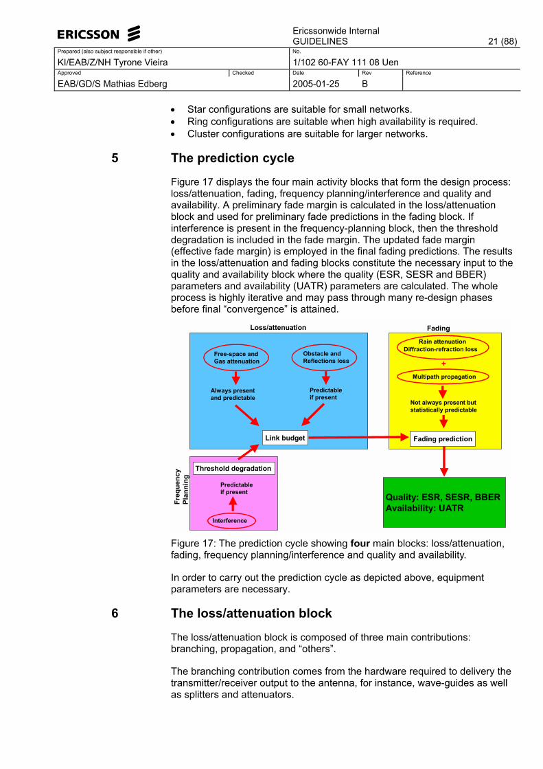
Figure 17 displays the four main activity blocks that form the design process: loss/attenuation, fading, frequency planning/interference and quality and availability. A preliminary fade margin is calculated in the loss/attenuation block and used for preliminary fade predictions in the fading block. If interference is present in the frequency-planning block, then the threshold degradation is included in the fade margin. The updated fade margin (effective fade margin) is employed in the final fading predictions. The results in the loss/attenuation and fading blocks constitute the necessary input to the quality and availability block where the quality (ESR, SESR and BBER) parameters and availability (UATR) parameters are calculated. The whole process is highly iterative and may pass through many re-design phases before final �convergence� is attained.
Interference
Predictableif present
Freq
uenc
yPl
anni
ng
Free-space and Gas attenuation
Always presentand predictable
Obstacle andReflections loss
Link budget
Predictableif present
Loss/attenuation
Not always present butstatistically predictable
Fading prediction
Rain attenuationDiffraction-refraction loss
Fading
Multipath propagation
+
Quality: ESR, SESR, BBERAvailability: UATR
Threshold degradation
Figure 17: The prediction cycle showing four main blocks: loss/attenuation, fading, frequency planning/interference and quality and availability.
In order to carry out the prediction cycle as depicted above, equipment parameters are necessary.
6 The loss/attenuation block
The loss/attenuation block is composed of three main contributions: branching, propagation, and �others�.
The branching contribution comes from the hardware required to delivery the transmitter/receiver output to the antenna, for instance, wave-guides as well as splitters and attenuators.
Ericssonwide Internal
GUIDELINES 22 (88)Prepared (also subject responsible if other) No.
KI/EAB/Z/NH Tyrone Vieira 1/102 60-FAY 111 08 Uen Approved Checked Date Rev Reference
EAB/GD/S Mathias Edberg 2005-01-25 B
The propagation contribution comes from the losses due to the Earth�s atmosphere and the terrain, for instance, free-space as well as gas, precipitation (mainly rain), ground reflection, and obstacle.
�Others� contributions have a somewhat unpredictable and sporadic character, for instance, sandstorm as well as fog, clouds, smoke, and moving objects crossing the path. In addition, poor equipment installation and unsuccessful antenna alignment may give rise to unpredictable losses. The �others� contributions is normally not calculated but can be accounted for in the planning process as an additional loss and then becoming part of the link budget.
6.1 Free-space loss
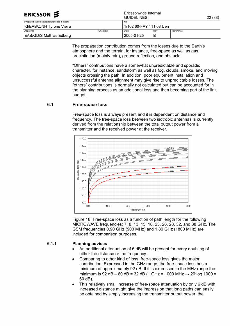
Free-space loss is always present and it is dependent on distance and frequency. The free-space loss between two isotropic antennas is currently derived from the relationship between the total output power from a transmitter and the received power at the receiver.
80.0
90.0
100.0
110.0
120.0
130.0
140.0
150.0
160.0
170.0
0.0 10.0 20.0 30.0 40.0 50.0Path length (km)
Free
-spa
ce lo
ss (d
B)
0.9 GHz
38 GHz
1.8 GHz
Figure 18: Free-space loss as a function of path length for the following MICROWAVE frequencies: 7, 8, 13, 15, 18, 23, 26, 28, 32, and 38 GHz. The GSM frequencies 0.90 GHz (900 MHz) and 1.80 GHz (1800 MHz) are included for comparison purposes.
6.1.1 Planning advices • An additional attenuation of 6 dB will be present for every doubling of
either the distance or the frequency. • Comparing to other kind of loss, free-space loss gives the major
contribution. Expressed in the GHz range, the free-space loss has a minimum of approximately 92 dB. If it is expressed in the MHz range the minimum is 92 dB � 60 dB = 32 dB (1 GHz = 1000 MHz → 20·log 1000 = 60 dB).
• This relatively small increase of free-space attenuation by only 6 dB with increased distance might give the impression that long paths can easily be obtained by simply increasing the transmitter output power, the
Ericssonwide Internal
GUIDELINES 23 (88)Prepared (also subject responsible if other) No.
KI/EAB/Z/NH Tyrone Vieira 1/102 60-FAY 111 08 Uen Approved Checked Date Rev Reference
EAB/GD/S Mathias Edberg 2005-01-25 B
receiver sensitivity, or the antenna gain. This is not so easy to accomplish because the total path attenuation is also determined by other negative contributions, for example gas attenuation.
• RF-planners commonly refer to half-wave dipole antenna gains. Comparing to the above presentation for which the gain of an �ideal� isotropic antenna is 1 (0 dB), the gain of a half-wave dipole antenna is 1.64 (2.15 dB). Considering both stations of a radio link, the difference between free-space loss comparison using isotropic and half-wave dipole antennas is about 4.30 dB.
6.2 Vegetation Attenuation
MINI-LINK sites are planned for line-of-sight application. In some situations, however, line of sight is not attainable and the network designer has to face obstacles as clutter, terrain obstacles, and vegetation areas (or single trees). There are cases for which the vegetation can be employed as shielding against far interference (unwanted signals) from other radio stations, but that should be applied with some caution.
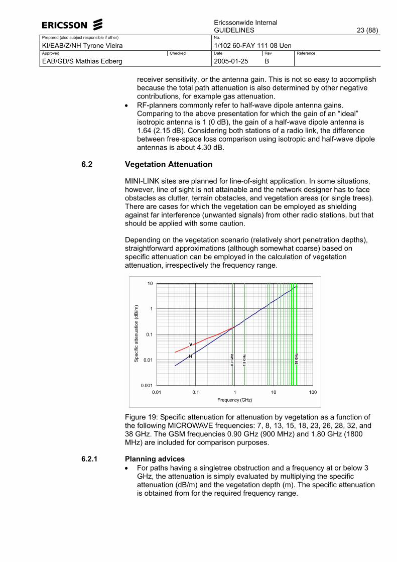
Depending on the vegetation scenario (relatively short penetration depths), straightforward approximations (although somewhat coarse) based on specific attenuation can be employed in the calculation of vegetation attenuation, irrespectively the frequency range.
0.001
0.01
0.1
1
10
0.01 0.1 1 10 100Frequency (GHz)
Spe
cific
atte
nuat
ion
(dB
/m)
V
H
0.9
GH
z
38 G
Hz
1.8
GH
z
Figure 19: Specific attenuation for attenuation by vegetation as a function of the following MICROWAVE frequencies: 7, 8, 13, 15, 18, 23, 26, 28, 32, and 38 GHz. The GSM frequencies 0.90 GHz (900 MHz) and 1.80 GHz (1800 MHz) are included for comparison purposes.
6.2.1 Planning advices • For paths having a singletree obstruction and a frequency at or below 3
GHz, the attenuation is simply evaluated by multiplying the specific attenuation (dB/m) and the vegetation depth (m). The specific attenuation is obtained from for the required frequency range.
Ericssonwide Internal
GUIDELINES 24 (88)Prepared (also subject responsible if other) No.
KI/EAB/Z/NH Tyrone Vieira 1/102 60-FAY 111 08 Uen Approved Checked Date Rev Reference
EAB/GD/S Mathias Edberg 2005-01-25 B
• At frequencies below 1 GHz, the attenuation seems to be more intensive for vertical polarization than for horizontal polarization. Tree branches affect long waves (low frequencies) more than tree leaves, and �pure diffraction� mechanism acting on the tree branches might start dominating over scattering.
• The use of vegetation as shield against interference signals might be an efficient strategy but the network designer should be aware that scattered trees in the terrain, as well as vast vegetation areas, could gradually be felled and therefore may lose the �shielding properties�.
• Depolarization (reduction of the cross-polarization discrimination) by vegetation seems to be dependent on the frequency and the vegetation depth. The higher the frequency, the more depolarization will be present. In addition, depolarization by vegetation increases with vegetation depth. In other words, cross-polarization discrimination (XPD) may be strongly reduced when using high frequencies in connection to larger vegetation depth, and vegetation may lose its �shielding properties�.
• For a singletree scenario (probably short vegetation depth), the model for the estimation of vegetation attenuation for f ≤ 3 GHz can be a reasonable straightforward method to make rough estimations of vegetation attenuation in the frequency range 6-38 GHz. In this case the vegetation attenuation for a given frequency is obtained by multiplying the specific attenuation (dB/m) as given in for the used frequency with the estimated vegetation depth (m).
• Although scenarios of trees without and with leaves might be considered, the focus should however be placed on the worst case, that is, whether the application is aimed to be used as interference shielding or as intentional transmission through vegetation. Interference shielding demands as much vegetation attenuation as possible and trees without leaves should be the worst case. Intentional transmission through vegetation demands as little vegetation attenuation as possible and trees with leaves should be the worst case.
• Vegetation is continuously growing. What seems to be LOS today might not be LOS �tomorrow�!
• The attenuation introduced by vegetation can be handled in TEMS LinkPlanner as an additional loss to be added to the calculated attenuation types like free-space, gas, and diffraction (obstacle) loss.
6.3 Gas attenuation
Nitrogen and oxygen molecules account for approximately 99% of the total volume of the atmosphere. Since the absorption bands of nitrogen is located far from the radio-relay region of the spectrum, the atmosphere is considered as being composed of a mixture of two �gases�: dry air (oxygen molecules) and water vapor (water molecules).
The two absorption peaks located in the frequency range of commercial radio links are located around 23 GHz (water molecules) and 50-70 GHz (oxygen molecules).
Ericssonwide Internal
GUIDELINES 25 (88)Prepared (also subject responsible if other) No.
KI/EAB/Z/NH Tyrone Vieira 1/102 60-FAY 111 08 Uen Approved Checked Date Rev Reference
EAB/GD/S Mathias Edberg 2005-01-25 B
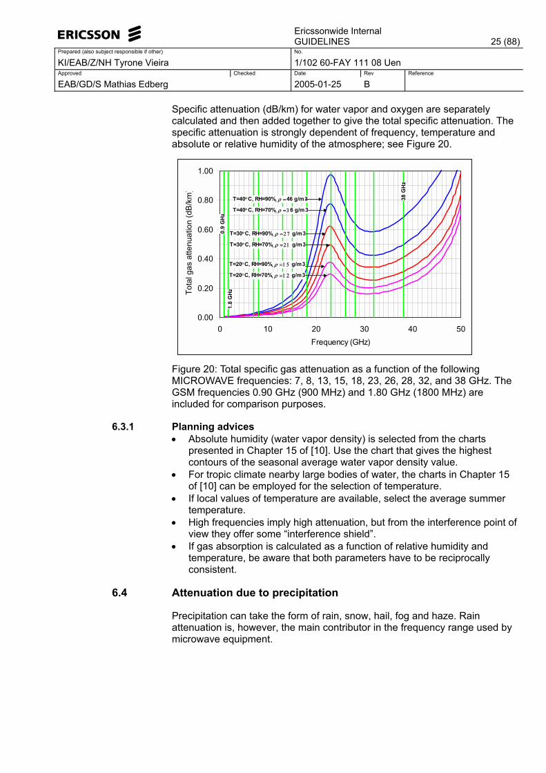
Specific attenuation (dB/km) for water vapor and oxygen are separately calculated and then added together to give the total specific attenuation. The specific attenuation is strongly dependent of frequency, temperature and absolute or relative humidity of the atmosphere; see Figure 20.
0.00
0.20
0.40
0.60
0.80
1.00
0 10 20 30 40 50Frequency (GHz)
Tota
l gas
atte
nuat
ion
(dB
/km
)
0.9
GH
z1.
8 G
Hz
38 G
Hz
T=40°C, RH=90%, ρ =46 g/m3
T=40°C, RH=70%, ρ =3 6 g/m3
T=30°C, RH=90%, ρ =2 7 g/m3
T=30°C, RH=70%, ρ =2 1 g/m3
T=20°C, RH=90%, ρ =1 5 g/m3
T=20°C, RH=70%, ρ =1 2 g/m3
Figure 20: Total specific gas attenuation as a function of the following MICROWAVE frequencies: 7, 8, 13, 15, 18, 23, 26, 28, 32, and 38 GHz. The GSM frequencies 0.90 GHz (900 MHz) and 1.80 GHz (1800 MHz) are included for comparison purposes.
6.3.1 Planning advices • Absolute humidity (water vapor density) is selected from the charts
presented in Chapter 15 of [10]. Use the chart that gives the highest contours of the seasonal average water vapor density value.
• For tropic climate nearby large bodies of water, the charts in Chapter 15 of [10] can be employed for the selection of temperature.
• If local values of temperature are available, select the average summer temperature.
• High frequencies imply high attenuation, but from the interference point of view they offer some �interference shield�.
• If gas absorption is calculated as a function of relative humidity and temperature, be aware that both parameters have to be reciprocally consistent.
6.4 Attenuation due to precipitation
Precipitation can take the form of rain, snow, hail, fog and haze. Rain attenuation is, however, the main contributor in the frequency range used by microwave equipment.
Ericssonwide Internal
GUIDELINES 26 (88)Prepared (also subject responsible if other) No.
KI/EAB/Z/NH Tyrone Vieira 1/102 60-FAY 111 08 Uen Approved Checked Date Rev Reference
EAB/GD/S Mathias Edberg 2005-01-25 B
0.01
0.1
1
10
100
0.1 1 10 100
Frequency (GHz)
Spe
cific
atte
nuat
ion
(dB
/km
)
0.9
GH
z
1.8
GH
z
7 G
Hz
38 G
Hz
0.25 mm/h
1.25 mm/h
5 mm/h
25 mm/h50 mm/h100 mm/h150 mm/h
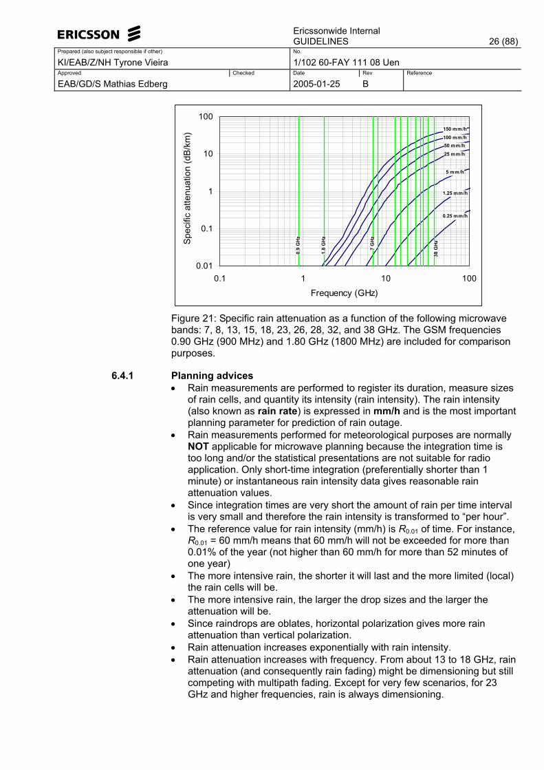
Figure 21: Specific rain attenuation as a function of the following microwave bands: 7, 8, 13, 15, 18, 23, 26, 28, 32, and 38 GHz. The GSM frequencies 0.90 GHz (900 MHz) and 1.80 GHz (1800 MHz) are included for comparison purposes.
6.4.1 Planning advices • Rain measurements are performed to register its duration, measure sizes
of rain cells, and quantity its intensity (rain intensity). The rain intensity (also known as rain rate) is expressed in mm/h and is the most important planning parameter for prediction of rain outage.
• Rain measurements performed for meteorological purposes are normally NOT applicable for microwave planning because the integration time is too long and/or the statistical presentations are not suitable for radio application. Only short-time integration (preferentially shorter than 1 minute) or instantaneous rain intensity data gives reasonable rain attenuation values.
• Since integration times are very short the amount of rain per time interval is very small and therefore the rain intensity is transformed to �per hour�.
• The reference value for rain intensity (mm/h) is R0.01 of time. For instance, R0.01 = 60 mm/h means that 60 mm/h will not be exceeded for more than 0.01% of the year (not higher than 60 mm/h for more than 52 minutes of one year)
• The more intensive rain, the shorter it will last and the more limited (local) the rain cells will be.
• The more intensive rain, the larger the drop sizes and the larger the attenuation will be.
• Since raindrops are oblates, horizontal polarization gives more rain attenuation than vertical polarization.
• Rain attenuation increases exponentially with rain intensity. • Rain attenuation increases with frequency. From about 13 to 18 GHz, rain
attenuation (and consequently rain fading) might be dimensioning but still competing with multipath fading. Except for very few scenarios, for 23 GHz and higher frequencies, rain is always dimensioning.
Ericssonwide Internal
GUIDELINES 27 (88)Prepared (also subject responsible if other) No.
KI/EAB/Z/NH Tyrone Vieira 1/102 60-FAY 111 08 Uen Approved Checked Date Rev Reference
EAB/GD/S Mathias Edberg 2005-01-25 B
• The contribution due to rain attenuation is NOT included in the link budget. It is only used in the calculation of rain fading.
6.5 Attenuation due to obstacles
Diffraction is the responsible mechanism for obstacle attenuation/loss. In fact, obstacle attenuation is also known in the literature as �diffraction attenuation/loss�.
For maximum performance, microwave equipment requires line-of-sight (LOS). If LOS is not attained, the single-peak method based on the knife-edge approximation as given by Figure 23, is normally applied for rough estimations of obstacle attenuation.
The estimation of obstacle attenuation can be performed in accordance to the following steps:
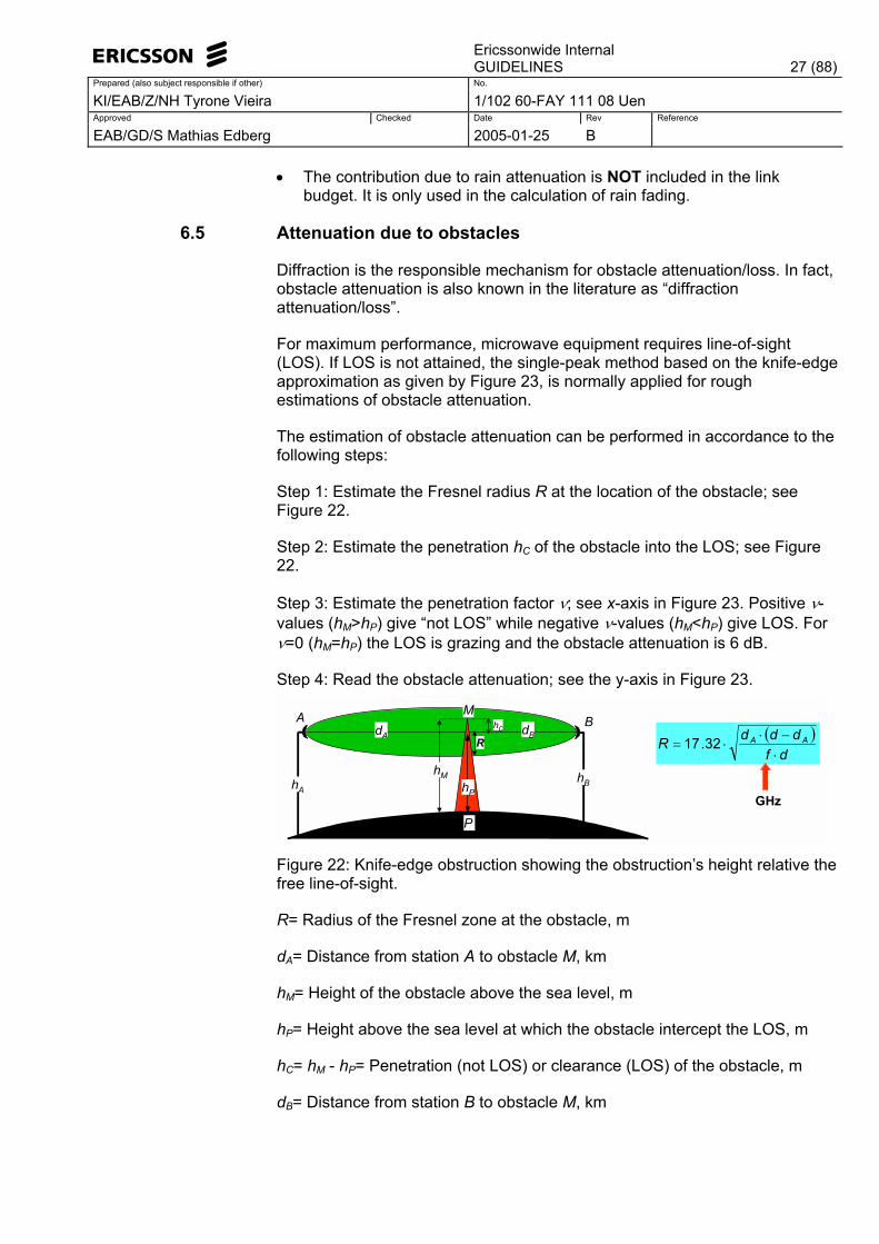
Step 1: Estimate the Fresnel radius R at the location of the obstacle; see Figure 22.
Step 2: Estimate the penetration hC of the obstacle into the LOS; see Figure 22.
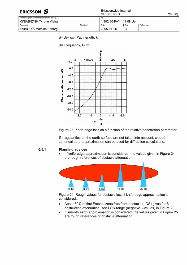
Step 3: Estimate the penetration factor ν; see x-axis in Figure 23. Positive ν-values (hM>hP) give �not LOS� while negative ν-values (hM<hP) give LOS. For ν=0 (hM=hP) the LOS is grazing and the obstacle attenuation is 6 dB.
Step 4: Read the obstacle attenuation; see the y-axis in Figure 23.
hAhB
M
hM
A B
hP
P
RhC ( )
dfdddR AA
⋅−⋅
⋅= 3217 .
GHz
dA dB
Figure 22: Knife-edge obstruction showing the obstruction�s height relative the free line-of-sight.
R= Radius of the Fresnel zone at the obstacle, m
dA= Distance from station A to obstacle M, km
hM= Height of the obstacle above the sea level, m
hP= Height above the sea level at which the obstacle intercept the LOS, m
hC= hM - hP= Penetration (not LOS) or clearance (LOS) of the obstacle, m
dB= Distance from station B to obstacle M, km
Ericssonwide Internal
GUIDELINES 28 (88)Prepared (also subject responsible if other) No.
KI/EAB/Z/NH Tyrone Vieira 1/102 60-FAY 111 08 Uen Approved Checked Date Rev Reference
EAB/GD/S Mathias Edberg 2005-01-25 B
d= dA+ dB= Path length, km
d= Frequency, GHz
0 -1.0 -2.01.02.0
0.0
-4.0
-8.0
-12.0
-16.0
-20.0
-24.0
4.0 LOSNot LOSO
bsta
cle
atte
nuat
ion,
dB
ν =R
hC
Gra
zing
Figure 23: Knife-edge loss as a function of the relative penetration parameter.
If irregularities on the earth surface are not taken into account, smooth spherical earth approximation can be used for diffraction calculations.
6.5.1 Planning advices • If knife-edge approximation is considered, the values given in Figure 24
are rough references of obstacle attenuation.
0 dB 0 dB 6 dB 16 dB 20 dB Figure 24: Rough values for obstacle loss if knife-edge approximation is considered. • About 60% of first Fresnel zone free from obstacle (LOS) gives 0 dB
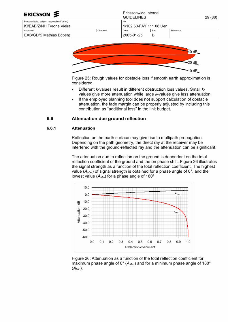
obstruction attenuation, see LOS-range (negative ν-values) in Figure 23. • If smooth earth approximation is considered, the values given in Figure 25
are rough references of obstacle attenuation.
Ericssonwide Internal
GUIDELINES 29 (88)Prepared (also subject responsible if other) No.
KI/EAB/Z/NH Tyrone Vieira 1/102 60-FAY 111 08 Uen Approved Checked Date Rev Reference
EAB/GD/S Mathias Edberg 2005-01-25 B
10 dB
20 dB
40 dB
Figure 25: Rough values for obstacle loss if smooth earth approximation is considered. • Different k-values result in different obstruction loss values. Small k-
values give more attenuation while large k-values give less attenuation. • If the employed planning tool does not support calculation of obstacle
attenuation, the fade margin can be properly adjusted by including this contribution as �additional loss� in the link budget.
6.6 Attenuation due ground reflection
6.6.1 Attenuation
Reflection on the earth surface may give rise to multipath propagation. Depending on the path geometry, the direct ray at the receiver may be interfered with the ground-reflected ray and the attenuation can be significant.
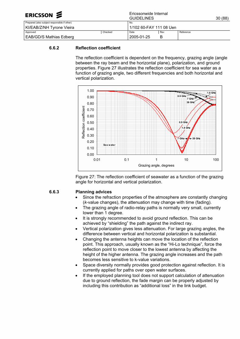
The attenuation due to reflection on the ground is dependent on the total reflection coefficient of the ground and the on phase shift. Figure 26 illustrates the signal strength as a function of the total reflection coefficient. The highest value (AMax) of signal strength is obtained for a phase angle of 0°, and the lowest value (AMin) for a phase angle of 180°.
-60.0
-50.0
-40.0
-30.0
-20.0
-10.0
0.0
10.0
0.0 0.1 0.2 0.3 0.4 0.5 0.6 0.7 0.8 0.9 1.0Reflection coefficient
Atte
nuat
ion,
dB
A max
Amin
Figure 26: Attenuation as a function of the total reflection coefficient for maximum phase angle of 0° (AMax) and for a minimum phase angle of 180° (AMin).
Ericssonwide Internal
GUIDELINES 30 (88)Prepared (also subject responsible if other) No.
KI/EAB/Z/NH Tyrone Vieira 1/102 60-FAY 111 08 Uen Approved Checked Date Rev Reference
EAB/GD/S Mathias Edberg 2005-01-25 B
6.6.2 Reflection coefficient
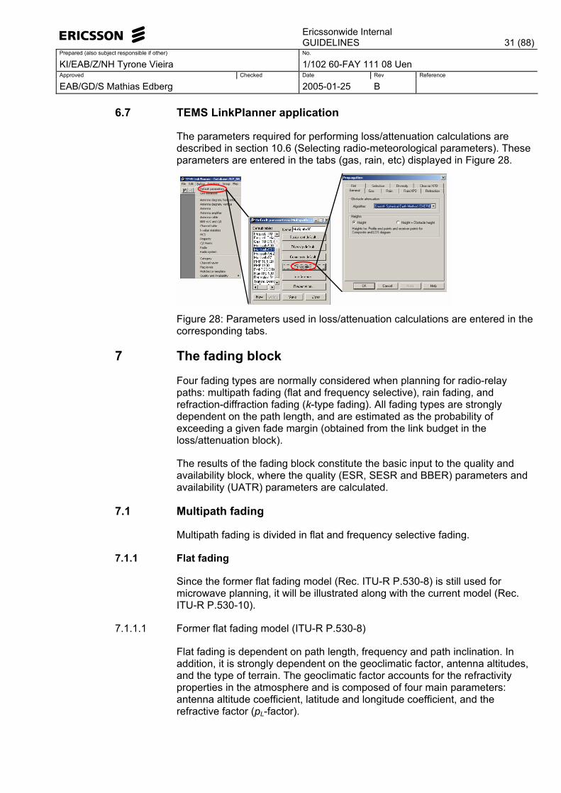
The reflection coefficient is dependent on the frequency, grazing angle (angle between the ray beam and the horizontal plane), polarization, and ground properties. Figure 27 illustrates the reflection coefficient for sea water as a function of grazing angle, two different frequencies and both horizontal and vertical polarization.
0.00
0.10
0.20
0.30
0.40
0.50
0.60
0.70
0.80
0.90
1.00
0.01 0.1 1 10 100Grazing angle, degrees
Ref
lect
ion
coef
ficie
nt
0.9 GHz
1.8 GHz
7 GHz 38 GHz
0.9 GHz1.8 GHz
7 GHz38 GHz
Sea water
Figure 27: The reflection coefficient of seawater as a function of the grazing angle for horizontal and vertical polarization.
6.6.3 Planning advices • Since the refraction properties of the atmosphere are constantly changing
(k-value changes), the attenuation may change with time (fading). • The grazing angle of radio-relay paths is normally very small, currently
lower than 1 degree. • It is strongly recommended to avoid ground reflection. This can be
achieved by �shielding� the path against the indirect ray. • Vertical polarization gives less attenuation. For large grazing angles, the
difference between vertical and horizontal polarization is substantial. • Changing the antenna heights can move the location of the reflection
point. This approach, usually known as the �Hi-Lo technique�, force the reflection point to move closer to the lowest antenna by affecting the height of the higher antenna. The grazing angle increases and the path becomes less sensitive to k-value variations.
• Space diversity normally provides good protection against reflection. It is currently applied for paths over open water surfaces.
• If the employed planning tool does not support calculation of attenuation due to ground reflection, the fade margin can be properly adjusted by including this contribution as �additional loss� in the link budget.
Ericssonwide Internal
GUIDELINES 31 (88)Prepared (also subject responsible if other) No.
KI/EAB/Z/NH Tyrone Vieira 1/102 60-FAY 111 08 Uen Approved Checked Date Rev Reference
EAB/GD/S Mathias Edberg 2005-01-25 B
6.7 TEMS LinkPlanner application
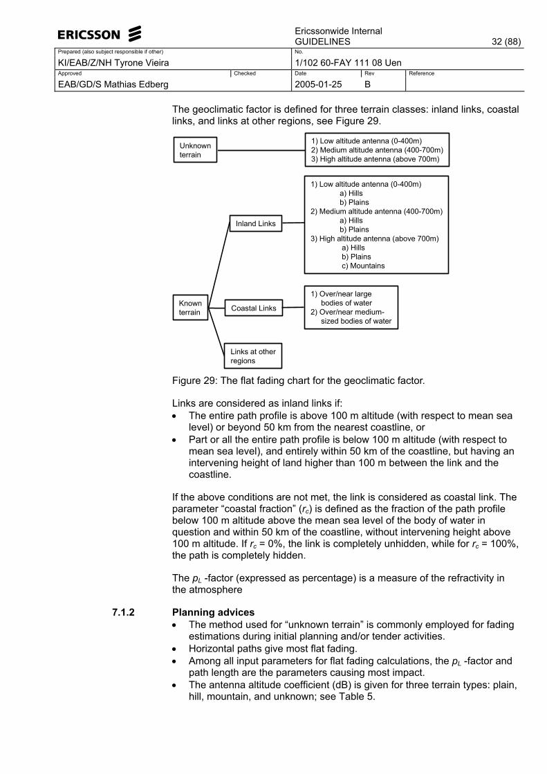
The parameters required for performing loss/attenuation calculations are described in section 10.6 (Selecting radio-meteorological parameters). These parameters are entered in the tabs (gas, rain, etc) displayed in Figure 28.
Figure 28: Parameters used in loss/attenuation calculations are entered in the corresponding tabs.
7 The fading block
Four fading types are normally considered when planning for radio-relay paths: multipath fading (flat and frequency selective), rain fading, and refraction-diffraction fading (k-type fading). All fading types are strongly dependent on the path length, and are estimated as the probability of exceeding a given fade margin (obtained from the link budget in the loss/attenuation block).
The results of the fading block constitute the basic input to the quality and availability block, where the quality (ESR, SESR and BBER) parameters and availability (UATR) parameters are calculated.
7.1 Multipath fading
Multipath fading is divided in flat and frequency selective fading.
7.1.1 Flat fading
Since the former flat fading model (Rec. ITU-R P.530-8) is still used for microwave planning, it will be illustrated along with the current model (Rec. ITU-R P.530-10).
7.1.1.1 Former flat fading model (ITU-R P.530-8)
Flat fading is dependent on path length, frequency and path inclination. In addition, it is strongly dependent on the geoclimatic factor, antenna altitudes, and the type of terrain. The geoclimatic factor accounts for the refractivity properties in the atmosphere and is composed of four main parameters: antenna altitude coefficient, latitude and longitude coefficient, and the refractive factor (pL-factor).
Ericssonwide Internal
GUIDELINES 32 (88)Prepared (also subject responsible if other) No.
KI/EAB/Z/NH Tyrone Vieira 1/102 60-FAY 111 08 Uen Approved Checked Date Rev Reference
EAB/GD/S Mathias Edberg 2005-01-25 B
The geoclimatic factor is defined for three terrain classes: inland links, coastal links, and links at other regions, see Figure 29.
Unknownterrain
Knownterrain
1) Low altitude antenna (0-400m)2) Medium altitude antenna (400-700m)3) High altitude antenna (above 700m)
Coastal Links
Inland Links
Links at otherregions
1) Over/near large bodies of water2) Over/near medium- sized bodies of water
1) Low altitude antenna (0-400m) a) Hills b) Plains2) Medium altitude antenna (400-700m) a) Hills b) Plains3) High altitude antenna (above 700m) a) Hills b) Plains c) Mountains
Figure 29: The flat fading chart for the geoclimatic factor.
Links are considered as inland links if: • The entire path profile is above 100 m altitude (with respect to mean sea
level) or beyond 50 km from the nearest coastline, or • Part or all the entire path profile is below 100 m altitude (with respect to
mean sea level), and entirely within 50 km of the coastline, but having an intervening height of land higher than 100 m between the link and the coastline.
If the above conditions are not met, the link is considered as coastal link. The parameter �coastal fraction� (rc) is defined as the fraction of the path profile below 100 m altitude above the mean sea level of the body of water in question and within 50 km of the coastline, without intervening height above 100 m altitude. If rc = 0%, the link is completely unhidden, while for rc = 100%, the path is completely hidden.
The pL -factor (expressed as percentage) is a measure of the refractivity in the atmosphere
7.1.2 Planning advices • The method used for �unknown terrain� is commonly employed for fading
estimations during initial planning and/or tender activities. • Horizontal paths give most flat fading. • Among all input parameters for flat fading calculations, the pL -factor and
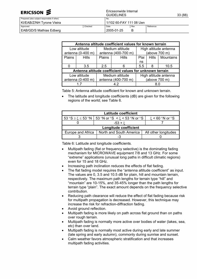
path length are the parameters causing most impact. • The antenna altitude coefficient (dB) is given for three terrain types: plain,
hill, mountain, and unknown; see Table 5.
Ericssonwide Internal
GUIDELINES 33 (88)Prepared (also subject responsible if other) No.
KI/EAB/Z/NH Tyrone Vieira 1/102 60-FAY 111 08 Uen Approved Checked Date Rev Reference
EAB/GD/S Mathias Edberg 2005-01-25 B
Antenna altitude coefficient values for known terrain
Low altitude antenna (0-400 m)
Medium altitude antenna (400-700 m)
High altitude antenna (above 700 m)
Plains Hills Plains Hills Plains
Hills Mountains
0 3.5 2.5 6 5.5 8 10.5 Antenna altitude coefficient values for unknown terrain
Low altitude antenna (0-400 m)
Medium altitude antenna (400-700 m)
High altitude antenna (above 700 m)
1.7 4.2 8.0
Table 5: Antenna altitude coefficient for known and unknown terrain. • The latitude and longitude coefficients (dB) are given for the following
regions of the world; see Table 6.
Latitude coefficient
53 °S ≥ ξ ≤ 53 °N 53 °N or °S < ξ < 53 °N or °S ξ < 60 °N or °S 0 -53 + ξ 7
Longitude coefficient Europe and Africa North and South America All other longitudes
3 -3 0
Table 6: Latitude and longitude coefficients. • Multipath fading (flat or frequency selective) is the dominating fading
mechanism for MICROWAVE equipment 7/8 and 13 GHz. For some �extreme� applications (unusual long paths in difficult climatic regions) even for 15 and 18 GHz.
• Increasing path inclination reduces the effects of flat fading. • The flat fading model requires the �antenna altitude coefficient� as input.
The values are 0, 3.5 and 10.5 dB for plain, hill and mountain terrain, respectively. The maximum path lengths for terrain type �hill� and �mountain� are 10-15%, and 35-45% longer than the path lengths for terrain type �plain�. The exact amount depends on the frequency selective contribution.
• Reducing path clearance will reduce the effect of flat fading because risk for multipath propagation is decreased. However, this technique may increase the risk for refraction-diffraction fading.
• Avoid ground reflection. • Multipath fading is more likely on path across flat ground than on paths
over rough terrain. • Multipath fading is normally more active over bodies of water (lakes, sea,
etc) than over land. • Multipath fading is normally most active during early and late summer
(late spring and early autumn), commonly during sunrise and sunset. • Calm weather favors atmospheric stratification and that increases
multipath fading activities.
Ericssonwide Internal
GUIDELINES 34 (88)Prepared (also subject responsible if other) No.
KI/EAB/Z/NH Tyrone Vieira 1/102 60-FAY 111 08 Uen Approved Checked Date Rev Reference
EAB/GD/S Mathias Edberg 2005-01-25 B
7.1.2.1 Current flat fading model (Rec. ITU-R P.530-10)
The terrain classes and the geoclimatic factor along with its �sub-parameters� antenna altitude coefficient, latitude and longitude coefficient, and the pL-factor, have been removed in the new flat fading model and substituted with the point refractivity gradient (see 10.6.3) that accounts for the refractivity properties of the atmosphere. In this particular sense, the model has been simplified although the selection of the point refractivity gradient directly from the charts given by the ITU-R may lead to substantial errors due to the current low resolution of the charts.
The point refractivity gradient is provided in a database in which the Earth surface is divided in a grid having a 1.5-degree resolution, that is, every square has a side of 1.5 degrees and for interpolation purposes each square can be considered as a plane (flat) square. The longitude and latitude of the Earth determine every point forming the grid and the values of the point refractivity gradient are given for every grid point. An interpolation procedure is required and that makes the new flat fading model difficult to use, but when implemented in microwave planning tools it is fast and powerful.
The most difficult aspect with the new flat fading model is, however, the parameter accounting for the interaction of the atmosphere with the terrain. It describes the standard deviation of terrain heights (expressed in meters) within a 110 km x 110 km area with a 30-second resolution. This parameter is obtained from a database covering the entire surface of the Earth, requiring a huge storage capacity. This makes the application even more complicated if the procedure is not implemented in a planning tool.
The new flat fading model has two options: 1) quick link design (with point refractivity gradient but without the terrain parameter) and detailed link design (with both point refractivity gradient and terrain parameter).
7.1.3 Frequency selective fading
Frequency selective fading implies amplitude and group delay distortions across the channel bandwidth. It affects particularly medium and high capacity radio links (> 32 Mbit/s).
The equipment signature is a measure of the receiver's capability to suppress the time-delayed signal. The signature is therefore the level of the signal that is necessary to obtain a certain BER (currently referred to 10-3 and/or 10-6) in the presence of an interfering signal with a pre-defined delay. This capability is measured in the laboratory.

Ericssonwide Internal
GUIDELINES 35 (88)Prepared (also subject responsible if other) No.
KI/EAB/Z/NH Tyrone Vieira 1/102 60-FAY 111 08 Uen Approved Checked Date Rev Reference
EAB/GD/S Mathias Edberg 2005-01-25 B
Since the amplitude of the reflected signal can be lower or higher than the direct signal, minimum or non-minimum phase group can be obtained. The phase-difference between the direct and indirect signals causes a notch (dip) at one of the frequency positions inside the spectrum bandwidth. By changing the phase difference between the direct and indirect signal, the "notch frequency" will change inside the bandwidth. At every notch frequency the signal is attenuated until the threshold for a specific BER (10-3 and/or 10-6) is exceeded. The notch depth and signature width for different MINI-LINK equipment are given in [3], [4] and [5] respectively.
The following parameters are employed in the estimation of frequency selective fading: • Normalization exponent (n): this parameter gives the exponent of a
typical path echo delay relationship (empirical). The value of the normalization exponent is in the range of 1.3 and 1.5. It is recommended to use 1.5.
• Mean relative delay (τm0): This parameter expresses the mean value of the relative delay (paths are relative to a standard length of 50 km). Typical values for the mean relative delay are in the range of 0.5 ns and 1.0 ns. It is recommended to use 0.7 ns.
• Constant factor (C⋅pb): This constant is strongly connected to the probability density functions (pdf) for applied time delay. Typical values for this constant are in the range of 1.0 and 4.0. It is recommended to use 2.16.
• Signature width: It is defined as the difference between the highest and lowest notch frequency.
• Signature height: This parameter is also known as �notch depth� and gives how insensitive the receiver is to changes in the phase difference of the direct and indirect signal for keeping a certain BER constant.
• Time delay: It is the time delay between the direct and indirect signals. A time delay of 6.3 s is normally applied in laboratory measurements.
7.1.4 Planning advices • As a rough rule, for bandwidth less than 40 MHz and path lengths shorter
than approximately 30 km, multipath fading is dominated by flat fading instead of frequency selective.
• Increasing the output power in order to reduce the outage time for selective fading doesn�t give any improvement. It only increases the flat fading or reduces the thermal noise power received without having any influence on the effects (amplitude and group delay distortions across the channel) of selective fading.
• The signature figures for wider microwave links give the worst case. Given the same Q&A objectives and overall assumptions, the signature figures of High Capacity links makes the path lengths for Medium Capacity links at most 13% shorter.
• The larger the fade margin, the less the flat fading contribution, the less the �multipath activity factor� and the larger is the relative difference between flat and frequency selective fading. Consequently the total fading is almost given by frequency selective fading, which is not directly dependent on the fade margin.
Ericssonwide Internal
GUIDELINES 36 (88)Prepared (also subject responsible if other) No.
KI/EAB/Z/NH Tyrone Vieira 1/102 60-FAY 111 08 Uen Approved Checked Date Rev Reference
EAB/GD/S Mathias Edberg 2005-01-25 B
7.2 Rain fading
The extent of the attenuation due to rain is primarily a function of the form and the size distribution of the raindrops. Rain events are statistically predictable with reasonable accuracy if short-integration or instantaneously rain measurements are available. Models that are based on measured cumulative distributions of rain events are currently employed in the prediction of the probability that a certain fade margin will be exceeded.
The model estimates the time (normally expressed in percentage of a year) during which a given fade depth (fade margin) is exceeded. Next, the result is converted to worst-month statistic. The concept of worst month for a certain specific value of the worst month is defined as that month with the highest probability of exceeding that specific value.
In the former rain-fading model, the main parameter (rainrate for 0.01% of time) is directly selected from the ITU-R charts by choosing the appropriate rain zones. In the current model, the parameter rainrate is obtained likewise the point refractivity gradient described in section 7.1.2.1. Similarly, an interpolation procedure is required, which makes the current rain-fading model difficult to use, but when implemented in microwave planning tools it is fast and powerful.
7.2.1 Planning advices • Other forms of precipitation (snow, hail, fog and haze) do not affect radio-
relay links as much as rain events and can therefore be considered as negligible.
• Rain fading starts increasing noticeably for microwave 18 GHz and normally dominates the total outage picture for microwave equipment of higher frequencies. For some �extreme� applications (unusual long paths in heavy rain regions having R0.01>100 mm/h) rain fading may be dimensioning even for 15 GHz or 13 GHz.
• Snow covering antennas and radomes, so-called ice coating, can result in two problems: increased attenuation and deformation of the antenna�s radiation pattern.
7.3 Refraction-Diffraction fading
Refraction-diffraction fading, also known as k-type fading, is characterized by seasonal and daily variations of the earth-radius factor k. For low k-values, the earth surface becomes more curved and terrain irregularities, man-made structures, and other objects, may intercept the Fresnel zones. For high k-values, the earth surface gets close to a plane surface and better LOS (lower antenna heights) is obtained.
The probability of refraction-diffraction fading is therefore indirectly connected to obstruction attenuation for a given value of earth-radius factor. Since the earth-radius factor is not constant, the probability of refraction-diffraction fading is calculated based on cumulative distributions of the earth-radius factor.
Refraction-diffraction fading is calculated in 4 steps:
Ericssonwide Internal
GUIDELINES 37 (88)Prepared (also subject responsible if other) No.
KI/EAB/Z/NH Tyrone Vieira 1/102 60-FAY 111 08 Uen Approved Checked Date Rev Reference
EAB/GD/S Mathias Edberg 2005-01-25 B
• A table containing probabilities that the various k-values will not be exceeded is firstly constructed. Then, a k-value distribution table for any specific pL factor is employed, in order to interpolate the probabilities for given k-values.
• Obstruction attenuation (using suitable model) values for the given k-values in the above table are calculated.
• The calculated obstruction attenuation values in the previous steps will then replace the k-values in the table. The former table (step 1) is transformed into a new table containing the probabilities in which the different obstruction attenuation values will be exceeded.
• The fade margin is coupled to obtained obstruction attenuation by applying the link budget. The probability that different fade margin values will be exceeded is finally calculated.
7.3.1 Planning advices • Diffraction-refraction fading is a path clearance procedure in which
antenna heights can by optimized for local climatic conditions. • Refraction-diffraction fading (k-type fading) is not considered in the quality
and availability calculations based on ITU-T G.826, G.827 and G.828, although it might be an important key to judge LOS-aspects (clearance) during special radiowave propagation conditions.
7.4 Outage due to cross-polar discrimination
The reduction of cross-polar discrimination (XPD) may strongly contribute to cause co-channel interference and to a lesser extent even adjacent channel interference. Since XPD is a powerful �parameter� commonly applied in frequency planning (re-using the same channel with different polarization options � horizontal and vertical), the reduction of XPD is now included in the total fading picture.
The reduction of cross-polar discrimination (XPD) takes place when some of the energy propagated in one polarization is transferred to the orthogonal polarization and produces a signal, which causes interference in the receiver of the orthogonal polarized channel (cross-polarization interference).
Heavy rain and multipath fading are the main contributors to reduction of XPD and estimations of XPD are therefore performed for clear air and rain. In clear air, the reduction of XPD may be due to the depolarization of the signal caused by changes in the refractivity of the atmosphere along the transmission path, or by reflection from a tilted atmospheric layer, or even by scattering or reflection from the ground or water. During rain, the reduction of XPD arises due to reflection and scattering on the raindrops.
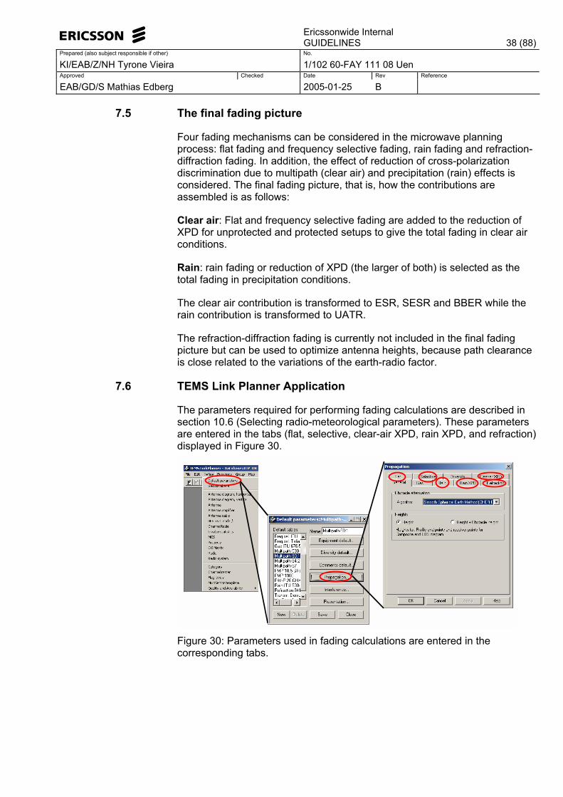
Ericssonwide Internal
GUIDELINES 38 (88)Prepared (also subject responsible if other) No.
KI/EAB/Z/NH Tyrone Vieira 1/102 60-FAY 111 08 Uen Approved Checked Date Rev Reference
EAB/GD/S Mathias Edberg 2005-01-25 B
7.5 The final fading picture
Four fading mechanisms can be considered in the microwave planning process: flat fading and frequency selective fading, rain fading and refraction-diffraction fading. In addition, the effect of reduction of cross-polarization discrimination due to multipath (clear air) and precipitation (rain) effects is considered. The final fading picture, that is, how the contributions are assembled is as follows:
Clear air: Flat and frequency selective fading are added to the reduction of XPD for unprotected and protected setups to give the total fading in clear air conditions.
Rain: rain fading or reduction of XPD (the larger of both) is selected as the total fading in precipitation conditions.
The clear air contribution is transformed to ESR, SESR and BBER while the rain contribution is transformed to UATR.
The refraction-diffraction fading is currently not included in the final fading picture but can be used to optimize antenna heights, because path clearance is close related to the variations of the earth-radio factor.
7.6 TEMS Link Planner Application
The parameters required for performing fading calculations are described in section 10.6 (Selecting radio-meteorological parameters). These parameters are entered in the tabs (flat, selective, clear-air XPD, rain XPD, and refraction) displayed in Figure 30.
Figure 30: Parameters used in fading calculations are entered in the corresponding tabs.
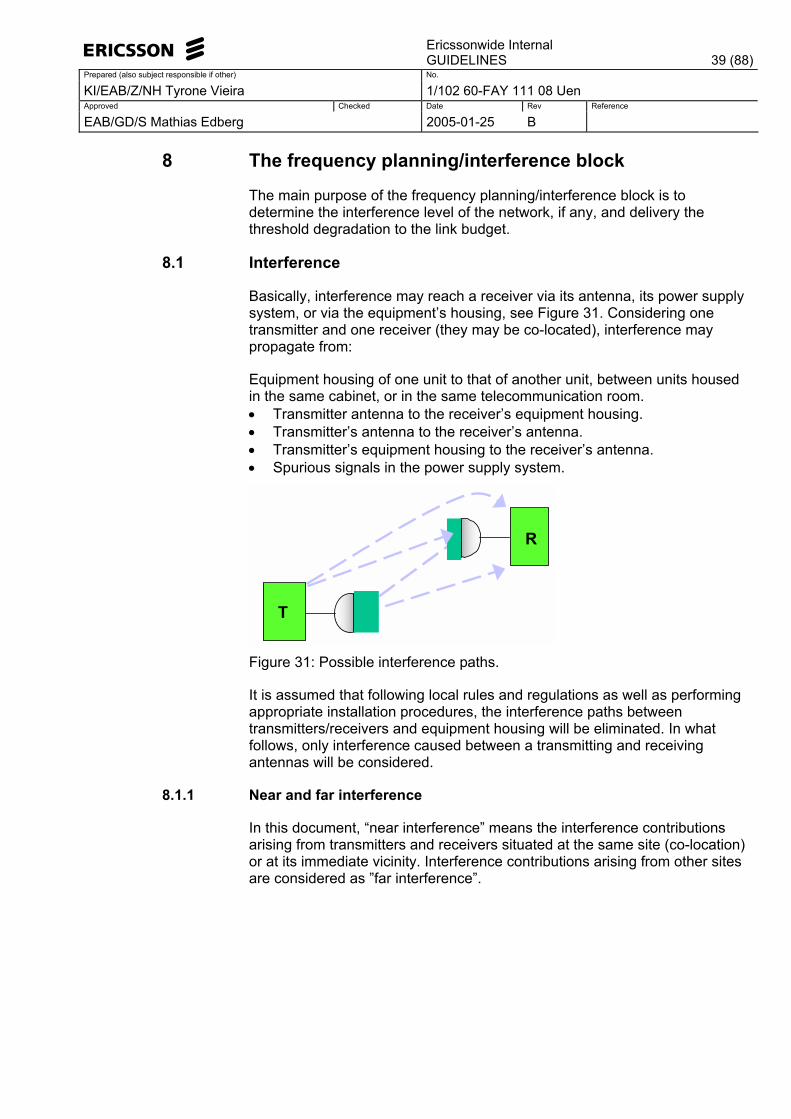
Ericssonwide Internal
GUIDELINES 39 (88)Prepared (also subject responsible if other) No.
KI/EAB/Z/NH Tyrone Vieira 1/102 60-FAY 111 08 Uen Approved Checked Date Rev Reference
EAB/GD/S Mathias Edberg 2005-01-25 B
8 The frequency planning/interference block
The main purpose of the frequency planning/interference block is to determine the interference level of the network, if any, and delivery the threshold degradation to the link budget.
8.1 Interference
Basically, interference may reach a receiver via its antenna, its power supply system, or via the equipment�s housing, see Figure 31. Considering one transmitter and one receiver (they may be co-located), interference may propagate from:
Equipment housing of one unit to that of another unit, between units housed in the same cabinet, or in the same telecommunication room. • Transmitter antenna to the receiver�s equipment housing. • Transmitter�s antenna to the receiver�s antenna. • Transmitter�s equipment housing to the receiver�s antenna. • Spurious signals in the power supply system.
T
R
Figure 31: Possible interference paths.
It is assumed that following local rules and regulations as well as performing appropriate installation procedures, the interference paths between transmitters/receivers and equipment housing will be eliminated. In what follows, only interference caused between a transmitting and receiving antennas will be considered.
8.1.1 Near and far interference
In this document, �near interference� means the interference contributions arising from transmitters and receivers situated at the same site (co-location) or at its immediate vicinity. Interference contributions arising from other sites are considered as �far interference�.
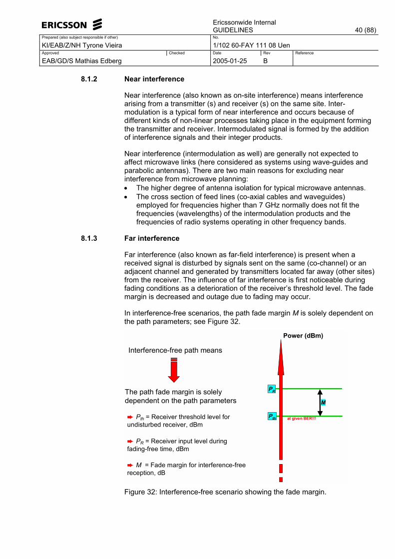
Ericssonwide Internal
GUIDELINES 40 (88)Prepared (also subject responsible if other) No.
KI/EAB/Z/NH Tyrone Vieira 1/102 60-FAY 111 08 Uen Approved Checked Date Rev Reference
EAB/GD/S Mathias Edberg 2005-01-25 B
8.1.2 Near interference
Near interference (also known as on-site interference) means interference arising from a transmitter (s) and receiver (s) on the same site. Inter- modulation is a typical form of near interference and occurs because of different kinds of non-linear processes taking place in the equipment forming the transmitter and receiver. Intermodulated signal is formed by the addition of interference signals and their integer products.
Near interference (intermodulation as well) are generally not expected to affect microwave links (here considered as systems using wave-guides and parabolic antennas). There are two main reasons for excluding near interference from microwave planning: • The higher degree of antenna isolation for typical microwave antennas. • The cross section of feed lines (co-axial cables and waveguides)
employed for frequencies higher than 7 GHz normally does not fit the frequencies (wavelengths) of the intermodulation products and the frequencies of radio systems operating in other frequency bands.
8.1.3 Far interference
Far interference (also known as far-field interference) is present when a received signal is disturbed by signals sent on the same (co-channel) or an adjacent channel and generated by transmitters located far away (other sites) from the receiver. The influence of far interference is first noticeable during fading conditions as a deterioration of the receiver�s threshold level. The fade margin is decreased and outage due to fading may occur.
In interference-free scenarios, the path fade margin M is solely dependent on the path parameters; see Figure 32.
Interference-free path means
The path fade margin is solelydependent on the path parameters
➨ M = Fade margin for interference-freereception, dB
➨ Pth = Receiver threshold level forundisturbed receiver, dBm
➨ PR = Receiver input level duringfading-free time, dBm
PR
at given BER!!!Pth
M
Power (dBm)
Figure 32: Interference-free scenario showing the fade margin.
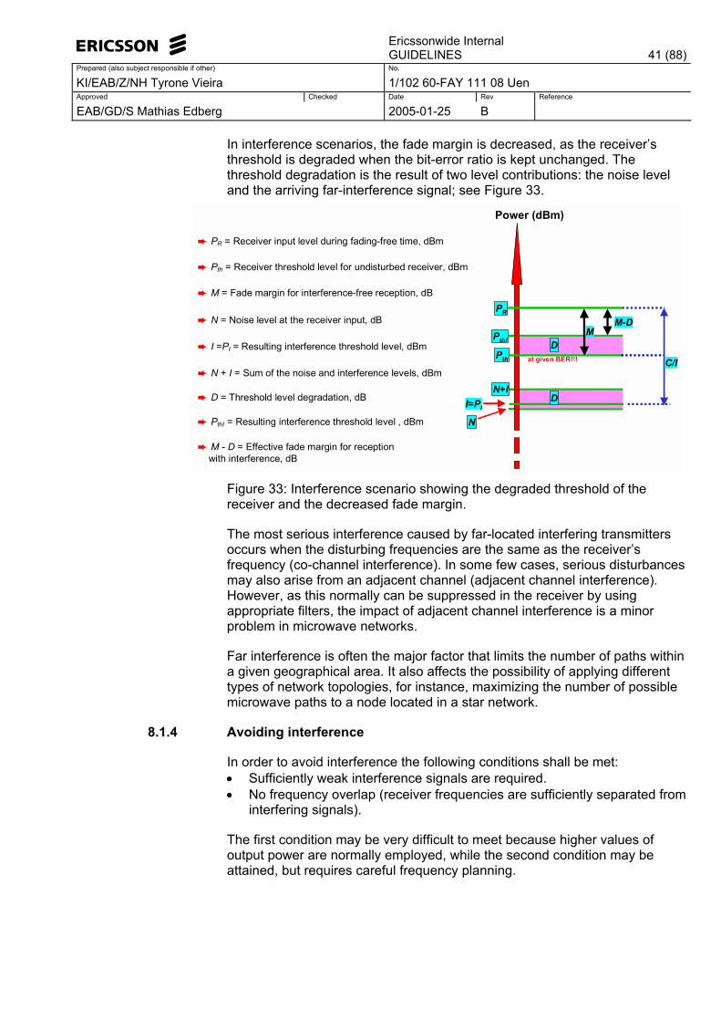
Ericssonwide Internal
GUIDELINES 41 (88)Prepared (also subject responsible if other) No.
KI/EAB/Z/NH Tyrone Vieira 1/102 60-FAY 111 08 Uen Approved Checked Date Rev Reference
EAB/GD/S Mathias Edberg 2005-01-25 B
In interference scenarios, the fade margin is decreased, as the receiver�s threshold is degraded when the bit-error ratio is kept unchanged. The threshold degradation is the result of two level contributions: the noise level and the arriving far-interference signal; see Figure 33.
N
N+I
DPthI
M-D
➨ I =PI = Resulting interference threshold level, dBm
➨ N = Noise level at the receiver input, dB
➨ N + I = Sum of the noise and interference levels, dBm
➨ D = Threshold level degradation, dB
PR
Pth
Power (dBm)
at given BER!!!
M
➨ PR = Receiver input level during fading-free time, dBm
➨ Pth = Receiver threshold level for undisturbed receiver, dBm
➨ M = Fade margin for interference-free reception, dB
➨ PthI = Resulting interference threshold level , dBm
➨ M - D = Effective fade margin for receptionwith interference, dB
I=PI
C/I
D
Figure 33: Interference scenario showing the degraded threshold of the receiver and the decreased fade margin.
The most serious interference caused by far-located interfering transmitters occurs when the disturbing frequencies are the same as the receiver�s frequency (co-channel interference). In some few cases, serious disturbances may also arise from an adjacent channel (adjacent channel interference). However, as this normally can be suppressed in the receiver by using appropriate filters, the impact of adjacent channel interference is a minor problem in microwave networks.
Far interference is often the major factor that limits the number of paths within a given geographical area. It also affects the possibility of applying different types of network topologies, for instance, maximizing the number of possible microwave paths to a node located in a star network.
8.1.4 Avoiding interference
In order to avoid interference the following conditions shall be met: • Sufficiently weak interference signals are required. • No frequency overlap (receiver frequencies are sufficiently separated from
interfering signals).
The first condition may be very difficult to meet because higher values of output power are normally employed, while the second condition may be attained, but requires careful frequency planning.
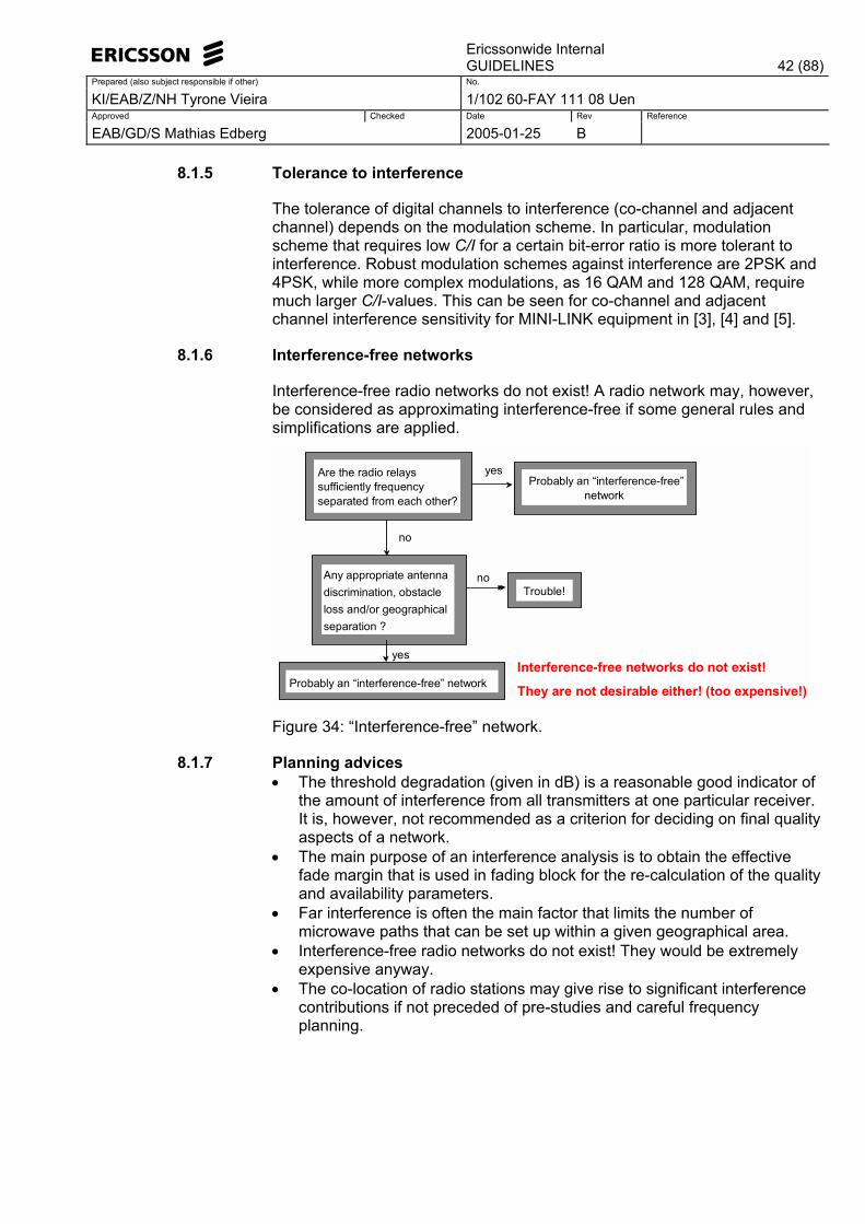
Ericssonwide Internal
GUIDELINES 42 (88)Prepared (also subject responsible if other) No.
KI/EAB/Z/NH Tyrone Vieira 1/102 60-FAY 111 08 Uen Approved Checked Date Rev Reference
EAB/GD/S Mathias Edberg 2005-01-25 B
8.1.5 Tolerance to interference
The tolerance of digital channels to interference (co-channel and adjacent channel) depends on the modulation scheme. In particular, modulation scheme that requires low C/I for a certain bit-error ratio is more tolerant to interference. Robust modulation schemes against interference are 2PSK and 4PSK, while more complex modulations, as 16 QAM and 128 QAM, require much larger C/I-values. This can be seen for co-channel and adjacent channel interference sensitivity for MINI-LINK equipment in [3], [4] and [5].
8.1.6 Interference-free networks
Interference-free radio networks do not exist! A radio network may, however, be considered as approximating interference-free if some general rules and simplifications are applied.
Are the radio relayssufficiently frequencyseparated from each other?
yes
no
Trouble!Any appropriate antennadiscrimination, obstacleloss and/or geographicalseparation ?
Probably an �interference-free� network
Probably an �interference-free�network
yes
no
Interference-free networks do not exist!
They are not desirable either! (too expensive!)
Figure 34: �Interference-free� network.
8.1.7 Planning advices • The threshold degradation (given in dB) is a reasonable good indicator of
the amount of interference from all transmitters at one particular receiver. It is, however, not recommended as a criterion for deciding on final quality aspects of a network.
• The main purpose of an interference analysis is to obtain the effective fade margin that is used in fading block for the re-calculation of the quality and availability parameters.
• Far interference is often the main factor that limits the number of microwave paths that can be set up within a given geographical area.
• Interference-free radio networks do not exist! They would be extremely expensive anyway.
• The co-location of radio stations may give rise to significant interference contributions if not preceded of pre-studies and careful frequency planning.

Ericssonwide Internal
GUIDELINES 43 (88)Prepared (also subject responsible if other) No.
KI/EAB/Z/NH Tyrone Vieira 1/102 60-FAY 111 08 Uen Approved Checked Date Rev Reference
EAB/GD/S Mathias Edberg 2005-01-25 B
8.2 Frequency planning of microwave networks
The objective of frequency planning of microwave networks is to assign as few frequencies as possible and in such a manner, that the quality and availability of the microwave paths are minimally affected by interference.
Frequency planning should rely on the concept of accomplishing the quality and availability objectives. The �3-dB threshold degradation approach� may lead to over dimensioning or under dimensioning. The threshold degradation may, however, give some clues on the degree of interference in the network
8.3 Terminology for frequency planning
Three words are currently used (and misused!) in frequency planning and frequency management: • Allocation (of a frequency band) is the frequency administration of a
frequency band for the purpose of its use by one or more services. This task is normally performed by the ITU.
• Allotment (of a radio frequency or radio frequency channel) is the frequency administration of required frequency channels of an agreed frequency plan adopted by a competent conference. These frequency channels are to be used by one or more Administrations in one or more countries or geographical regions.
• Assignment (of a radio frequency or radio frequency channel) is the authorization given by an Administration for a radio station to use a radio frequency or radio frequency channel under specified conditions.
Allotment and assignment are made in accordance with the Series F Recommendations given by the Study Group 9 of the ITU-R. The allotment consists of one or more alternative radio-frequency channel arrangements.
These arrangements are used in accordance to the rules of local Administrations in a country or geographical region. In most applications, however, frequency bands and frequency channels are already selected and provided to operators.
8.4 Channel arrangements
Channels are segments (subdivisions) of a frequency range (raster) or portion (frequency band) of the electromagnetic spectrum. Like every portion (frequency band), every channel has a specified bandwidth. Depending on the capacity of the link, a certain amount of carries can be accommodated into the band. For instance, a frequency raster may include four adjacent 28-MHz channels (applicable for 34 Mbit/s links), but each of these channels can be further divided in four 7 MHz channels (applicable for 8 Mbit/s). In order to enable four 7 MHz channels to be included within one 28 MHz channel, the centre frequencies of the 28 and the 7 MHz channels should not coincide. Likewise, each 7 MHz channel may be divided in two 3.5 MHz channels (applicable for 2 Mbit/s).
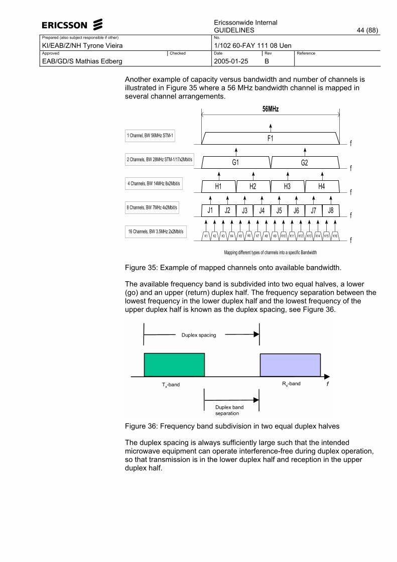
Ericssonwide Internal
GUIDELINES 44 (88)Prepared (also subject responsible if other) No.
KI/EAB/Z/NH Tyrone Vieira 1/102 60-FAY 111 08 Uen Approved Checked Date Rev Reference
EAB/GD/S Mathias Edberg 2005-01-25 B
Another example of capacity versus bandwidth and number of channels is illustrated in Figure 35 where a 56 MHz bandwidth channel is mapped in several channel arrangements.
f
f
f
f
f
G1
K1 K2 K3 K4 K5 K6 K7 K8 K9 K10 K11 K12 K13 K14 K15 K16
56MHz
F1
G2
H1 H2 H3 H4
J1 J2 J3 J4 J5 J6 J7 J8
1 Channel, BW 56MHz STM-1
2 Channels, BW 28MHz STM-1/17x2Mbit/s
4 Channels, BW 14MHz 8x2Mbit/s
8 Channels, BW 7MHz 4x2Mbit/s
16 Channels, BW 3.5MHz 2x2Mbit/s
Mapping different types of channels into a specific Bandwidth
Figure 35: Example of mapped channels onto available bandwidth.
The available frequency band is subdivided into two equal halves, a lower (go) and an upper (return) duplex half. The frequency separation between the lowest frequency in the lower duplex half and the lowest frequency of the upper duplex half is known as the duplex spacing, see Figure 36.
Rx-band f
Duplex bandseparation
Duplex spacing
Tx-band
Figure 36: Frequency band subdivision in two equal duplex halves
The duplex spacing is always sufficiently large such that the intended microwave equipment can operate interference-free during duplex operation, so that transmission is in the lower duplex half and reception in the upper duplex half.
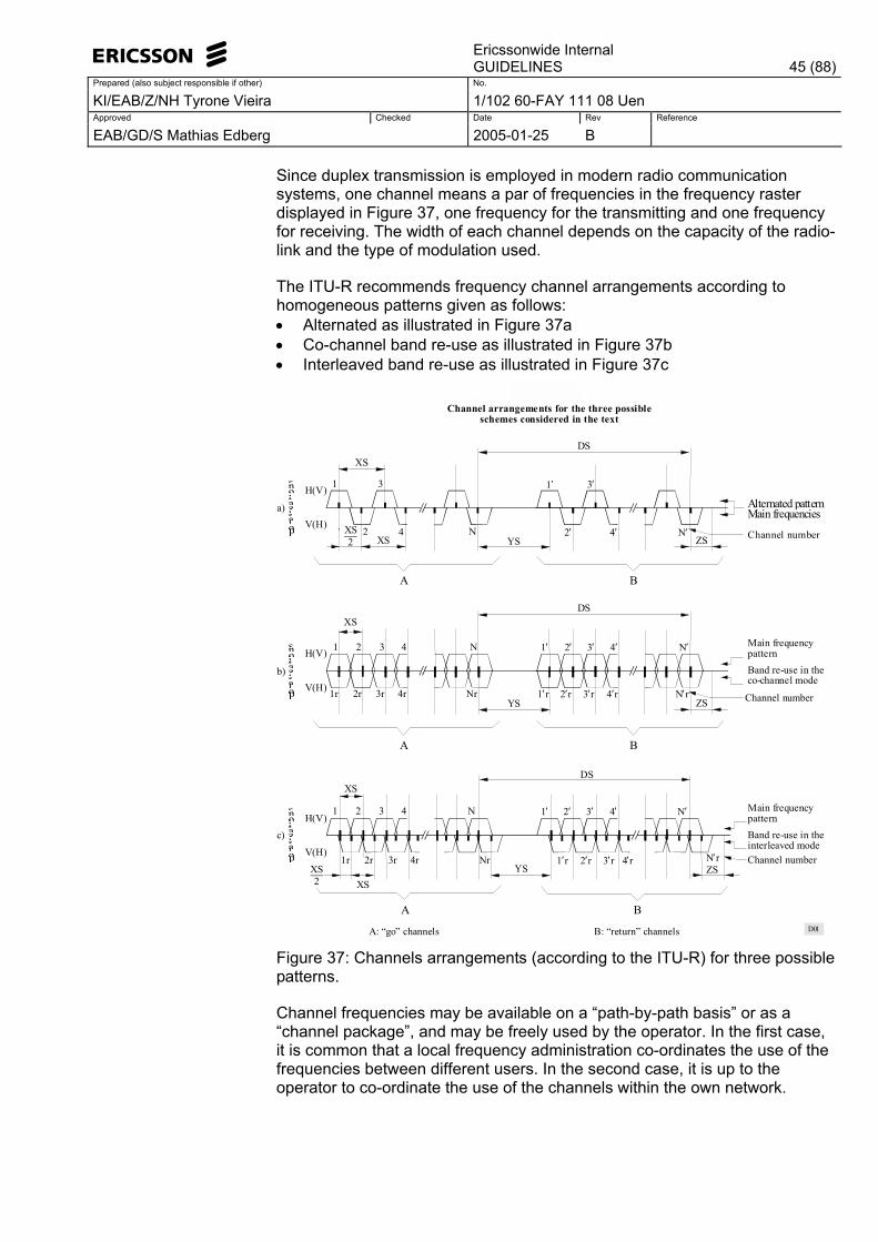
Ericssonwide Internal
GUIDELINES 45 (88)Prepared (also subject responsible if other) No.
KI/EAB/Z/NH Tyrone Vieira 1/102 60-FAY 111 08 Uen Approved Checked Date Rev Reference
EAB/GD/S Mathias Edberg 2005-01-25 B
Since duplex transmission is employed in modern radio communication systems, one channel means a par of frequencies in the frequency raster displayed in Figure 37, one frequency for the transmitting and one frequency for receiving. The width of each channel depends on the capacity of the radio-link and the type of modulation used.
The ITU-R recommends frequency channel arrangements according to homogeneous patterns given as follows: • Alternated as illustrated in Figure 37a • Co-channel band re-use as illustrated in Figure 37b • Interleaved band re-use as illustrated in Figure 37c
A B
A B
A B
Alternated patternMain frequencies
FIGURE 1Channel arrangements for the three possible
schemes considered in the text
Channel number
Main frequencypatternBand re-use in theco-channel mode
Channel number
Main frequencypatternBand re-use in theinterleaved modeChannel number
a)
b)
c)
Polarizations
Polarizations
Polarizations
H(V)
V(H)
H(V)
V(H)
H(V)
V(H)
XS
XSXS2
1 3
2 4 N
D01
1′ 3′
2′ 4′ N′ZSYS
XS
YS
DS
DS
N1 2 3 4
1r 2r 3r 4r Nr
N′1′ 2′ 3′ 4′
1′r 2′r 3′r 4′r N′rZS
XS
YS
DS
N1 2 3 4
1r 2r 3r 4r Nr
N′1′ 2′ 3′ 4′
1′r 2′r 3′r 4′r N′rZS
XSXS2
A: �go� channels B: �return� channels Figure 37: Channels arrangements (according to the ITU-R) for three possible patterns.
Channel frequencies may be available on a �path-by-path basis� or as a �channel package�, and may be freely used by the operator. In the first case, it is common that a local frequency administration co-ordinates the use of the frequencies between different users. In the second case, it is up to the operator to co-ordinate the use of the channels within the own network.
Ericssonwide Internal
GUIDELINES 46 (88)Prepared (also subject responsible if other) No.
KI/EAB/Z/NH Tyrone Vieira 1/102 60-FAY 111 08 Uen Approved Checked Date Rev Reference
EAB/GD/S Mathias Edberg 2005-01-25 B
Local frequency administrations normally keep the use of available frequency bands and the corresponding channel distribution in good order. Several operators may be forced to share the same frequency band, although different channels, thus making necessary to control planning parameters such as transmitted power, site co-ordinates, antenna heights, etc.
8.5 Channel width and spectral efficiency
The method of modulation and the capacity affect the required bandwidth and the interference tolerance of a radio-link. It is therefore always considered when a frequency raster is constructed. Sophisticated modulation methods (high levels of QAM and TCM) are required for high capacity links so more information can be packed together. In what follows, a few examples illustrate the procedure: • 2PSK has two states (0° and 180°). Shifting the carrier phase by 180°
requires 1 Hertz of the carrier frequency for each bit of the base band (21=2) and the spectral efficiency is 1 bit/s/Hz. A 2 Mbit/s base band modulated with 2 PSK requires a RF carrier with a bandwidth of 2 MHz. A 140 Mbit/s base band requires a RF carrier that has a bandwidth of 140 MHz.
• 8PSK has eight states in steps of 45°. Shifting the carrier phase by 45° requires 1 Hertz of the carrier frequency for 3 bits of the base band (23=8) and the spectral efficiency is 3 bit/s/Hz. A 2 Mbit/s base band modulated with 8PSK requires a RF carrier with a bandwidth of 0.67 MHz. A 140 Mbit/s base band requires a RF carrier that has a bandwidth of 47 MHz.
• 16QAM has 16 states (phase and amplitude are shifted). One shift requires 1 Hertz of the carrier frequency for 4 bits of the base band (24=16) and the spectral efficiency is 4 bit/s/Hz. A 2 Mbit/s base band modulated with 16QAM requires a RF carrier with a bandwidth of 0.50 MHz. A 140 Mbit/s base band requires a RF carrier that has a bandwidth of 35 MHz.
• 128QAM has 128 states (phase and amplitude are shifted). One shift requires 1 Hertz of the carrier frequency for 7 bits of the base band (27=128) and the spectral efficiency is 7 bit/s/Hz. A 2 Mbit/s base band modulated with 128QAM requires a RF carrier with a bandwidth of 0.28 MHz. A 140 Mbit/s base band requires a RF carrier that has a bandwidth of 20 MHz.
8.6 Channel spacing for high capacity SDH links
MINI-LINK High Capacity (SDH) links of STM-1 and multiple STM-1 capacities may operate in the same frequency band and with the same channel arrangements as current MINI-LINK Medium Capacity (PDH) links. This is only possible by choosing higher levels of modulation than usual (spectral efficiency is improved).
Examples of possible channel arrangements allowing transmission of the basic STM-1 and multiple STM-1 within available radio-frequency channel plans are given in Table 7.
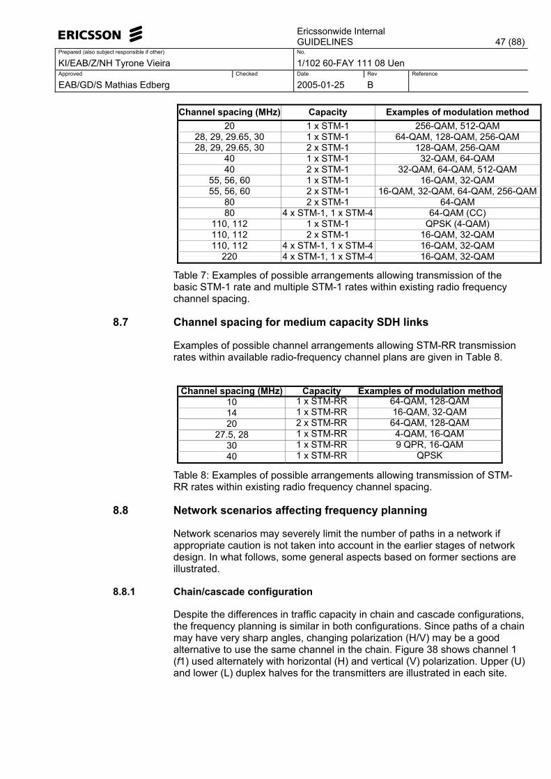
Ericssonwide Internal
GUIDELINES 47 (88)Prepared (also subject responsible if other) No.
KI/EAB/Z/NH Tyrone Vieira 1/102 60-FAY 111 08 Uen Approved Checked Date Rev Reference
EAB/GD/S Mathias Edberg 2005-01-25 B
Channel spacing (MHz) Capacity Examples of modulation method 20 1 x STM-1 256-QAM, 512-QAM
28, 29, 29.65, 30 1 x STM-1 64-QAM, 128-QAM, 256-QAM 28, 29, 29.65, 30 2 x STM-1 128-QAM, 256-QAM
40 1 x STM-1 32-QAM, 64-QAM 40 2 x STM-1 32-QAM, 64-QAM, 512-QAM
55, 56, 60 1 x STM-1 16-QAM, 32-QAM 55, 56, 60 2 x STM-1 16-QAM, 32-QAM, 64-QAM, 256-QAM
80 2 x STM-1 64-QAM 80 4 x STM-1, 1 x STM-4 64-QAM (CC)
110, 112 1 x STM-1 QPSK (4-QAM) 110, 112 2 x STM-1 16-QAM, 32-QAM 110, 112 4 x STM-1, 1 x STM-4 16-QAM, 32-QAM
220 4 x STM-1, 1 x STM-4 16-QAM, 32-QAM
Table 7: Examples of possible arrangements allowing transmission of the basic STM-1 rate and multiple STM-1 rates within existing radio frequency channel spacing.
8.7 Channel spacing for medium capacity SDH links
Examples of possible channel arrangements allowing STM-RR transmission rates within available radio-frequency channel plans are given in Table 8.
Channel spacing (MHz) Capacity Examples of modulation method
10 1 x STM-RR 64-QAM, 128-QAM 14 1 x STM-RR 16-QAM, 32-QAM 20 2 x STM-RR 64-QAM, 128-QAM
27.5, 28 1 x STM-RR 4-QAM, 16-QAM 30 1 x STM-RR 9 QPR, 16-QAM 40 1 x STM-RR QPSK
Table 8: Examples of possible arrangements allowing transmission of STM-RR rates within existing radio frequency channel spacing.
8.8 Network scenarios affecting frequency planning
Network scenarios may severely limit the number of paths in a network if appropriate caution is not taken into account in the earlier stages of network design. In what follows, some general aspects based on former sections are illustrated.
8.8.1 Chain/cascade configuration
Despite the differences in traffic capacity in chain and cascade configurations, the frequency planning is similar in both configurations. Since paths of a chain may have very sharp angles, changing polarization (H/V) may be a good alternative to use the same channel in the chain. Figure 38 shows channel 1 (f1) used alternately with horizontal (H) and vertical (V) polarization. Upper (U) and lower (L) duplex halves for the transmitters are illustrated in each site.
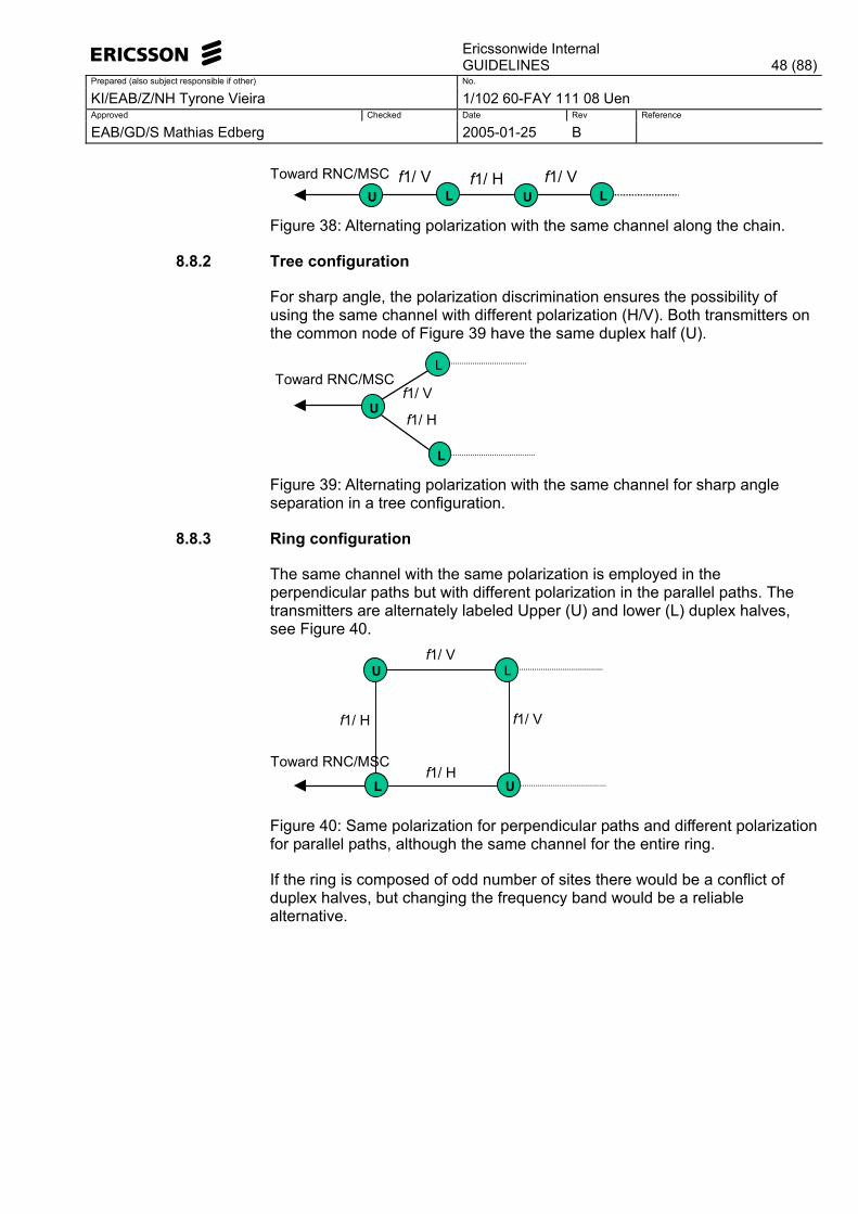
Ericssonwide Internal
GUIDELINES 48 (88)Prepared (also subject responsible if other) No.
KI/EAB/Z/NH Tyrone Vieira 1/102 60-FAY 111 08 Uen Approved Checked Date Rev Reference
EAB/GD/S Mathias Edberg 2005-01-25 B
f1/ V f1/ H f1/ VToward RNC/MSCU L U L
Figure 38: Alternating polarization with the same channel along the chain.
8.8.2 Tree configuration
For sharp angle, the polarization discrimination ensures the possibility of using the same channel with different polarization (H/V). Both transmitters on the common node of Figure 39 have the same duplex half (U).
Toward RNC/MSC
f1/ V
f1/ HU
L
L Figure 39: Alternating polarization with the same channel for sharp angle separation in a tree configuration.
8.8.3 Ring configuration
The same channel with the same polarization is employed in the perpendicular paths but with different polarization in the parallel paths. The transmitters are alternately labeled Upper (U) and lower (L) duplex halves, see Figure 40.
U L
UL
Toward RNC/MSC
f1/ V
f1/ V
f1/ H
f1/ H
Figure 40: Same polarization for perpendicular paths and different polarization for parallel paths, although the same channel for the entire ring.
If the ring is composed of odd number of sites there would be a conflict of duplex halves, but changing the frequency band would be a reliable alternative.
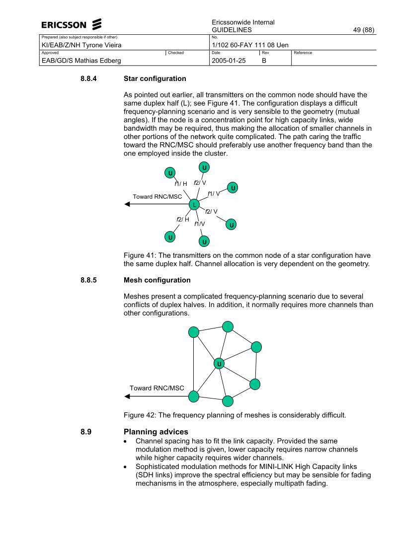
Ericssonwide Internal
GUIDELINES 49 (88)Prepared (also subject responsible if other) No.
KI/EAB/Z/NH Tyrone Vieira 1/102 60-FAY 111 08 Uen Approved Checked Date Rev Reference
EAB/GD/S Mathias Edberg 2005-01-25 B
8.8.4 Star configuration
As pointed out earlier, all transmitters on the common node should have the same duplex half (L); see Figure 41. The configuration displays a difficult frequency-planning scenario and is very sensible to the geometry (mutual angles). If the node is a concentration point for high capacity links, wide bandwidth may be required, thus making the allocation of smaller channels in other portions of the network quite complicated. The path caring the traffic toward the RNC/MSC should preferably use another frequency band than the one employed inside the cluster.
UU
L
U
U
UU
Toward RNC/MSC
f1/ H f2/ V
f1/ V
f2/ V
f1/Vf2/ H
Figure 41: The transmitters on the common node of a star configuration have the same duplex half. Channel allocation is very dependent on the geometry.
8.8.5 Mesh configuration
Meshes present a complicated frequency-planning scenario due to several conflicts of duplex halves. In addition, it normally requires more channels than other configurations.
Toward RNC/MSC
U
Figure 42: The frequency planning of meshes is considerably difficult.
8.9 Planning advices • Channel spacing has to fit the link capacity. Provided the same
modulation method is given, lower capacity requires narrow channels while higher capacity requires wider channels.
• Sophisticated modulation methods for MINI-LINK High Capacity links (SDH links) improve the spectral efficiency but may be sensible for fading mechanisms in the atmosphere, especially multipath fading.
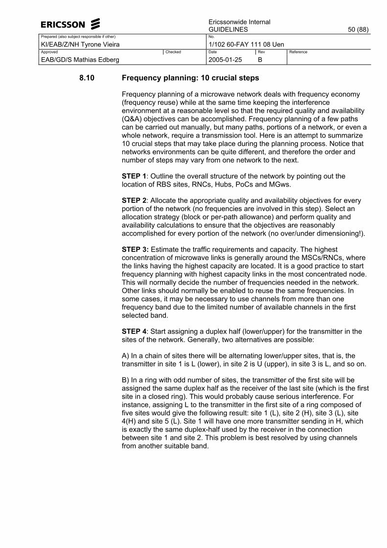
Ericssonwide Internal
GUIDELINES 50 (88)Prepared (also subject responsible if other) No.
KI/EAB/Z/NH Tyrone Vieira 1/102 60-FAY 111 08 Uen Approved Checked Date Rev Reference
EAB/GD/S Mathias Edberg 2005-01-25 B
8.10 Frequency planning: 10 crucial steps
Frequency planning of a microwave network deals with frequency economy (frequency reuse) while at the same time keeping the interference environment at a reasonable level so that the required quality and availability (Q&A) objectives can be accomplished. Frequency planning of a few paths can be carried out manually, but many paths, portions of a network, or even a whole network, require a transmission tool. Here is an attempt to summarize 10 crucial steps that may take place during the planning process. Notice that networks environments can be quite different, and therefore the order and number of steps may vary from one network to the next.
STEP 1: Outline the overall structure of the network by pointing out the location of RBS sites, RNCs, Hubs, PoCs and MGws.
STEP 2: Allocate the appropriate quality and availability objectives for every portion of the network (no frequencies are involved in this step). Select an allocation strategy (block or per-path allowance) and perform quality and availability calculations to ensure that the objectives are reasonably accomplished for every portion of the network (no over/under dimensioning!).
STEP 3: Estimate the traffic requirements and capacity. The highest concentration of microwave links is generally around the MSCs/RNCs, where the links having the highest capacity are located. It is a good practice to start frequency planning with highest capacity links in the most concentrated node. This will normally decide the number of frequencies needed in the network. Other links should normally be enabled to reuse the same frequencies. In some cases, it may be necessary to use channels from more than one frequency band due to the limited number of available channels in the first selected band.
STEP 4: Start assigning a duplex half (lower/upper) for the transmitter in the sites of the network. Generally, two alternatives are possible:
A) In a chain of sites there will be alternating lower/upper sites, that is, the transmitter in site 1 is L (lower), in site 2 is U (upper), in site 3 is L, and so on.
B) In a ring with odd number of sites, the transmitter of the first site will be assigned the same duplex half as the receiver of the last site (which is the first site in a closed ring). This would probably cause serious interference. For instance, assigning L to the transmitter in the first site of a ring composed of five sites would give the following result: site 1 (L), site 2 (H), site 3 (L), site 4(H) and site 5 (L). Site 1 will have one more transmitter sending in H, which is exactly the same duplex-half used by the receiver in the connection between site 1 and site 2. This problem is best resolved by using channels from another suitable band.
Ericssonwide Internal
GUIDELINES 51 (88)Prepared (also subject responsible if other) No.
KI/EAB/Z/NH Tyrone Vieira 1/102 60-FAY 111 08 Uen Approved Checked Date Rev Reference
EAB/GD/S Mathias Edberg 2005-01-25 B
Transmitters using upper and lower duplex halves are sometimes forced to mix on the same site. In this case, near interference has to be evaluated. The main parameter in the evaluation of near interference is the isolation (antenna separation) between transmitters and receivers on the same site. In addition, the frequency separation and the receiver�s capability of blocking (filtering) unwanted signals may valuable in reducing the effect of near interference.
STEP 5: Consider antenna discrimination aspects in the early stages of frequency planning. For instance, in a common site (node/hub), the links having sufficient separation angles may use the same channels. In addition to angle separation, distance separation (coupling loss) between two antennas may also give a certain degree of discrimination.
STEP 6: Re-use frequencies and polarization as often as possible. That is, if one channel is assigned to a node, always try to assign the same channel for the other paths on the same node. Note that the required number of frequencies may depend on the order of allocation. Therefore, try other combinations to minimize the required number of frequencies.
STEP 7: Proceed with the next node. It should normally be possible to plan the next node with the same frequencies as used in the former node. If necessary, change frequency for a path that is aligned to a path using the same frequency and connected to the former node.
STEP 8: Perform a new quality and availability calculation (after the frequency allocation) and identify the paths that do not meet the quality and availability objectives. Far interference calculation is carried out and the receivers having relatively high threshold degradation values are probably a part of the paths not meeting the quality and availability objectives. Make the appropriate changes (polarization, channel, frequency band, antenna size, etc) and ensure that a new interference calculation gives lower threshold degradation values. There might be some situations in which higher output power of a transmitter may improve the quality and availability figures without considerable interference contributions to the network. These favorable situations are however not so common.
STEP 9: Repeat step 8 until the quality and availability objectives of all portions of the network are accomplished.
STEP 10: The total analysis is finished and the network will have the final parameter values (channels, polarization, antenna size, frequency band, etc) as given by the last iteration circle.
8.11 Planning advices • Frequency planning is not carried out with the purpose of avoiding
interference, rather to accomplish the quality and availability objectives of each path or chain of the network!
• Reuse frequencies, i.e., repeat the use of frequencies as often as possible! Good frequency economy is always encouraged!
• Use antennas having high front-to-back ratios and large side-lobe suppression. These result in both good frequency economy and, in the
Ericssonwide Internal
GUIDELINES 52 (88)Prepared (also subject responsible if other) No.
KI/EAB/Z/NH Tyrone Vieira 1/102 60-FAY 111 08 Uen Approved Checked Date Rev Reference
EAB/GD/S Mathias Edberg 2005-01-25 B
final analysis, good overall network-economy. High performance antennas may be a suitable alternative.
• Do not use higher output power than necessary! Start always frequency planning with the lowest available output power. Another frequency planning strategy is to start with higher output power but reduce it to an optimum level at which the quality and availability objectives of each path or chain are achieved.
• If the choice is between higher transmitter output power and larger antennas, choose (if possible) a larger antenna that concentrates the transmitted power in smaller lobes and a certain degree of interference may be avoided.
• Changing polarization is a very effective measure against interference for paths having sharp angles, while very ineffective for paths forming wide angles.
• As a general rule, near interference should be avoided as much as possible by strictly allocating the same upper or lower duplex half to all transmitters on the same site.
• When assigning specific channels to the individual paths in a network it is strongly recommended to start with high capacity paths (the paths demanding wider bandwidth).
• For all MINI-LINK equipment frequencies, the antenna discrimination increases rapidly with the separation angle, and is an extremely efficient factor in suppressing interference. Thus, if the two paths are not closely aligned in a common direction it is normally possible to reuse the same channel.
• Generally, interference problems in microwave networks are more severe for paths connected to a common node. For paths far from nodes, interference can normally be easily handled.
• Interfering signals are not ways in line of sight! Low k-values decrease the line of sight (demand higher antenna heights) but offer better protection against interference from other stations.
• Never mix transmitters (or receivers) using upper and lower duplex halves on the same site. All transmitters (or receivers) on one site should have the same duplex half!
• It is not economically feasible to achieve interference-free networks. • Frequency planning is NOT the goal; it is carried out with the purpose of
minimize the interference level in the network and thereby accomplishing the quality and availability objectives!
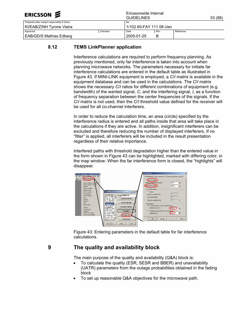
Ericssonwide Internal
GUIDELINES 53 (88)Prepared (also subject responsible if other) No.
KI/EAB/Z/NH Tyrone Vieira 1/102 60-FAY 111 08 Uen Approved Checked Date Rev Reference
EAB/GD/S Mathias Edberg 2005-01-25 B
8.12 TEMS LinkPlanner application
Interference calculations are required to perform frequency planning. As previously mentioned, only far interference is taken into account when planning microwave networks. The parameters necessary for initiate far interference calculations are entered in the default table as illustrated in Figure 43. If MINI-LINK equipment is employed, a C/I matrix is available in the equipment database and can be used in the calculations. The C/I matrix shows the necessary C/I ratios for different combinations of equipment (e.g. bandwidth) of the wanted signal, C, and the interfering signal, I, as a function of frequency separation between the center frequencies of the signals. If the C/I matrix is not used, then the C/I threshold value defined for the receiver will be used for all co-channel interferers.
In order to reduce the calculation time, an area (circle) specified by the interference radius is entered and all paths inside that area will take place in the calculations if they are active. In addition, insignificant interferers can be excluded and therefore reducing the number of displayed interferers. If no �filter� is applied, all interferers will be included in the result presentation regardless of their relative importance.
Interfered paths with threshold degradation higher than the entered value in the form shown in Figure 43 can be highlighted, marked with differing color, in the map window. When the far interference form is closed, the �highlights� will disappear.
Figure 43: Entering parameters in the default table for far interference calculations.
9 The quality and availability block
The main purpose of the quality and availability (Q&A) block is: • To calculate the quality (ESR, SESR and BBER) and unavailability
(UATR) parameters from the outage probabilities obtained in the fading block
• To set up reasonable Q&A objectives for the microwave path.
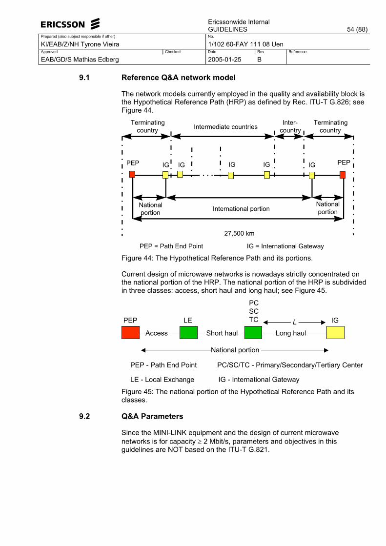
Ericssonwide Internal
GUIDELINES 54 (88)Prepared (also subject responsible if other) No.
KI/EAB/Z/NH Tyrone Vieira 1/102 60-FAY 111 08 Uen Approved Checked Date Rev Reference
EAB/GD/S Mathias Edberg 2005-01-25 B
9.1 Reference Q&A network model
The network models currently employed in the quality and availability block is the Hypothetical Reference Path (HRP) as defined by Rec. ITU-T G.826; see Figure 44.
IGIGIGIGIG PEPPEP
Nationalportion
Nationalportion International portion
PEP = Path End Point
27,500 km
Terminatingcountry
Inter-countryIntermediate countriesTerminating
country
IG = International Gateway Figure 44: The Hypothetical Reference Path and its portions.
Current design of microwave networks is nowadays strictly concentrated on the national portion of the HRP. The national portion of the HRP is subdivided in three classes: access, short haul and long haul; see Figure 45.
PEP IG
Access
LE
Short haul Long haul
PCSCTC
National portion
PEP - Path End Point
LE - Local Exchange
PC/SC/TC - Primary/Secondary/Tertiary Center
IG - International Gateway
L
Figure 45: The national portion of the Hypothetical Reference Path and its classes.
9.2 Q&A Parameters
Since the MINI-LINK equipment and the design of current microwave networks is for capacity ≥ 2 Mbit/s, parameters and objectives in this guidelines are NOT based on the ITU-T G.821.
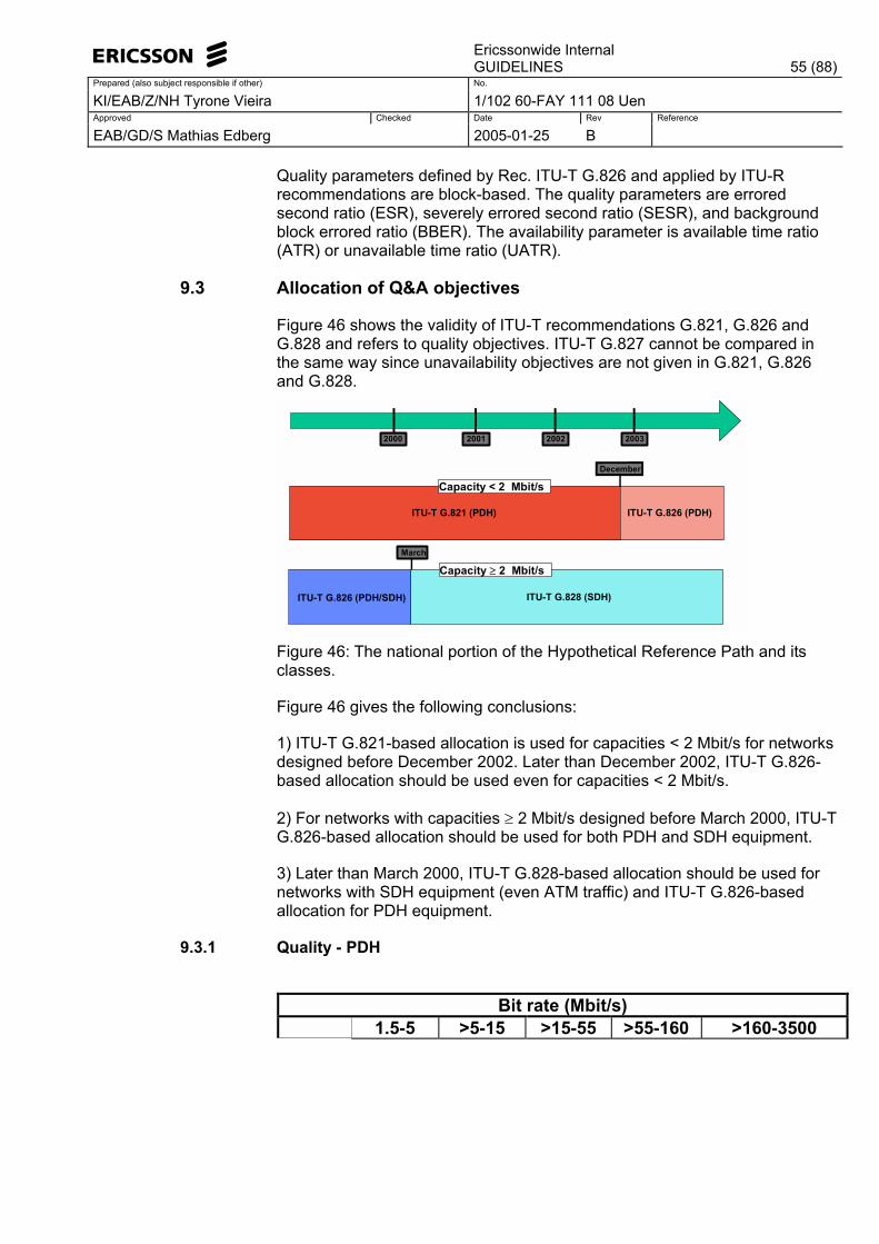
Ericssonwide Internal
GUIDELINES 55 (88)Prepared (also subject responsible if other) No.
KI/EAB/Z/NH Tyrone Vieira 1/102 60-FAY 111 08 Uen Approved Checked Date Rev Reference
EAB/GD/S Mathias Edberg 2005-01-25 B
Quality parameters defined by Rec. ITU-T G.826 and applied by ITU-R recommendations are block-based. The quality parameters are errored second ratio (ESR), severely errored second ratio (SESR), and background block errored ratio (BBER). The availability parameter is available time ratio (ATR) or unavailable time ratio (UATR).
9.3 Allocation of Q&A objectives
Figure 46 shows the validity of ITU-T recommendations G.821, G.826 and G.828 and refers to quality objectives. ITU-T G.827 cannot be compared in the same way since unavailability objectives are not given in G.821, G.826 and G.828.
2000 2001 2002 2003
Capacity < 2 Mbit/s
ITU-T G.821 (PDH) ITU-T G.826 (PDH)
December
Capacity ≥ 2 Mbit/s
ITU-T G.828 (SDH)ITU-T G.826 (PDH/SDH)
March
Figure 46: The national portion of the Hypothetical Reference Path and its classes.
Figure 46 gives the following conclusions:
1) ITU-T G.821-based allocation is used for capacities < 2 Mbit/s for networks designed before December 2002. Later than December 2002, ITU-T G.826-based allocation should be used even for capacities < 2 Mbit/s.
2) For networks with capacities ≥ 2 Mbit/s designed before March 2000, ITU-T G.826-based allocation should be used for both PDH and SDH equipment.
3) Later than March 2000, ITU-T G.828-based allocation should be used for networks with SDH equipment (even ATM traffic) and ITU-T G.826-based allocation for PDH equipment.
9.3.1 Quality - PDH
Bit rate (Mbit/s)
1.5-5 >5-15 >15-55 >55-160 >160-3500
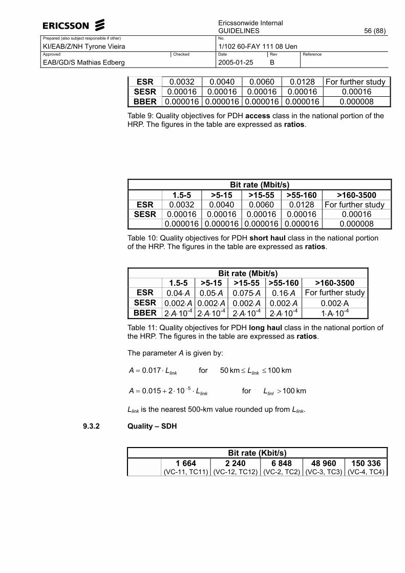
Ericssonwide Internal
GUIDELINES 56 (88)Prepared (also subject responsible if other) No.
KI/EAB/Z/NH Tyrone Vieira 1/102 60-FAY 111 08 Uen Approved Checked Date Rev Reference
EAB/GD/S Mathias Edberg 2005-01-25 B
ESR 0.0032 0.0040 0.0060 0.0128 For further studySESR 0.00016 0.00016 0.00016 0.00016 0.00016 BBER 0.000016 0.000016 0.000016 0.000016 0.000008
Table 9: Quality objectives for PDH access class in the national portion of the HRP. The figures in the table are expressed as ratios.
Bit rate (Mbit/s)
1.5-5 >5-15 >15-55 >55-160 >160-3500 ESR 0.0032 0.0040 0.0060 0.0128 For further study
SESR 0.00016 0.00016 0.00016 0.00016 0.00016 BBER 0.000016 0.000016 0.000016 0.000016 0.000008
Table 10: Quality objectives for PDH short haul class in the national portion of the HRP. The figures in the table are expressed as ratios.
Bit rate (Mbit/s)
1.5-5 >5-15 >15-55 >55-160 >160-3500 ESR 0.04⋅A 0.05⋅A 0.075⋅A 0.16⋅A For further study
SESR 0.002⋅A 0.002⋅A 0.002⋅A 0.002⋅A 0.002⋅A BBER 2⋅A⋅10-4 2⋅A⋅10-4 2⋅A⋅10-4 2⋅A⋅10-4 1⋅A⋅10-4
Table 11: Quality objectives for PDH long haul class in the national portion of the HRP. The figures in the table are expressed as ratios.
The parameter A is given by:
km 100 km 50 for 017.0 ≤≤⋅= linklink LLA
km 100 for 102015.0 5 >⋅⋅+= −linllink LLA
Llink is the nearest 500-km value rounded up from Llink.
9.3.2 Quality � SDH
Bit rate (Kbit/s)
1 664 (VC-11, TC11)
2 240 (VC-12, TC12)
6 848 (VC-2, TC2)
48 960 (VC-3, TC3)
150 336 (VC-4, TC4)
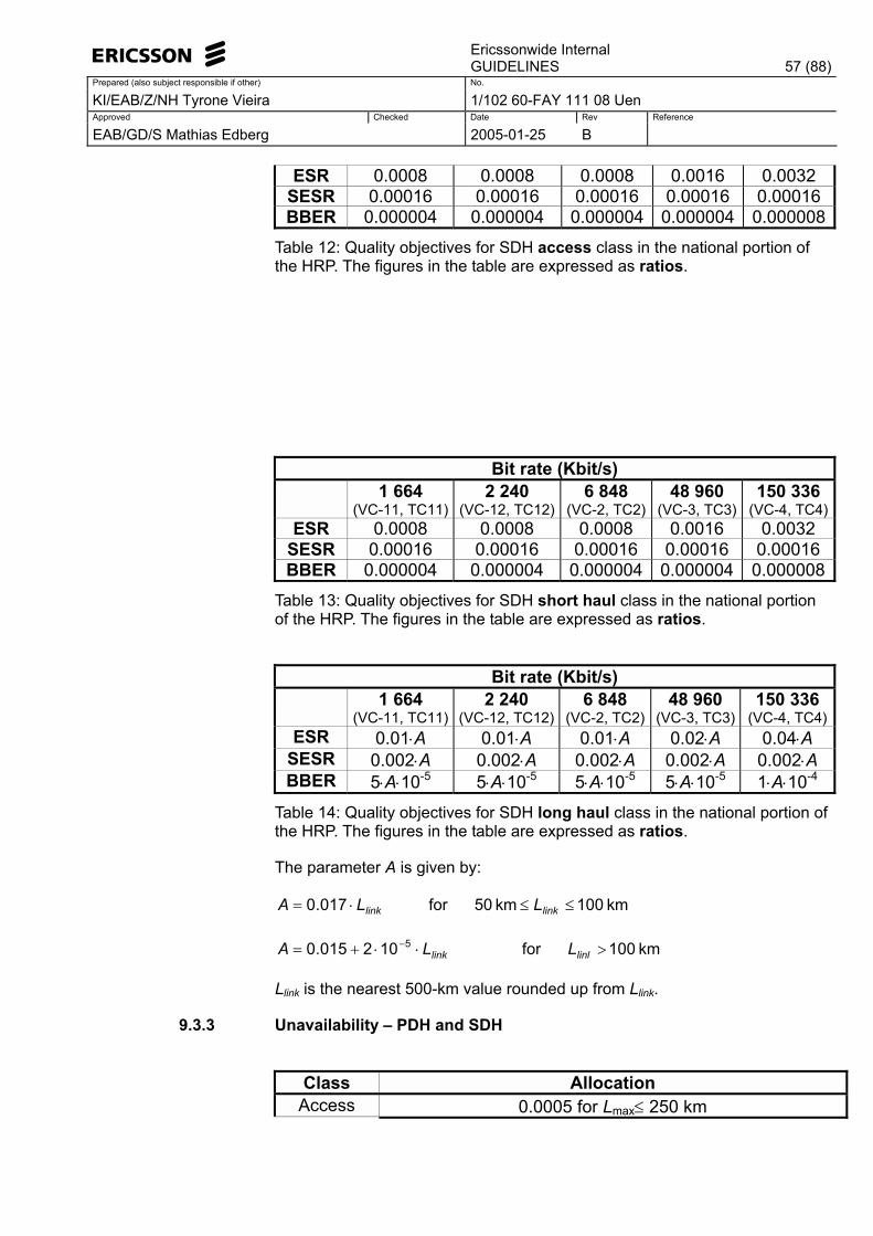
Ericssonwide Internal
GUIDELINES 57 (88)Prepared (also subject responsible if other) No.
KI/EAB/Z/NH Tyrone Vieira 1/102 60-FAY 111 08 Uen Approved Checked Date Rev Reference
EAB/GD/S Mathias Edberg 2005-01-25 B
ESR 0.0008 0.0008 0.0008 0.0016 0.0032 SESR 0.00016 0.00016 0.00016 0.00016 0.00016 BBER 0.000004 0.000004 0.000004 0.000004 0.000008
Table 12: Quality objectives for SDH access class in the national portion of the HRP. The figures in the table are expressed as ratios.
Bit rate (Kbit/s)
1 664 (VC-11, TC11)
2 240 (VC-12, TC12)
6 848 (VC-2, TC2)
48 960 (VC-3, TC3)
150 336 (VC-4, TC4)
ESR 0.0008 0.0008 0.0008 0.0016 0.0032 SESR 0.00016 0.00016 0.00016 0.00016 0.00016 BBER 0.000004 0.000004 0.000004 0.000004 0.000008
Table 13: Quality objectives for SDH short haul class in the national portion of the HRP. The figures in the table are expressed as ratios.
Bit rate (Kbit/s)
1 664 (VC-11, TC11)
2 240 (VC-12, TC12)
6 848 (VC-2, TC2)
48 960 (VC-3, TC3)
150 336 (VC-4, TC4)
ESR 0.01⋅A 0.01⋅A 0.01⋅A 0.02⋅A 0.04⋅A SESR 0.002⋅A 0.002⋅A 0.002⋅A 0.002⋅A 0.002⋅A BBER 5⋅A⋅10-5 5⋅A⋅10-5 5⋅A⋅10-5 5⋅A⋅10-5 1⋅A⋅10-4
Table 14: Quality objectives for SDH long haul class in the national portion of the HRP. The figures in the table are expressed as ratios.
The parameter A is given by:
km 100 km 50 for 017.0 ≤≤⋅= linklink LLA
km 100 for 102015.0 5 >⋅⋅+= −linllink LLA
Llink is the nearest 500-km value rounded up from Llink.
9.3.3 Unavailability � PDH and SDH
Class Allocation
Access 0.0005 for Lmax≤ 250 km
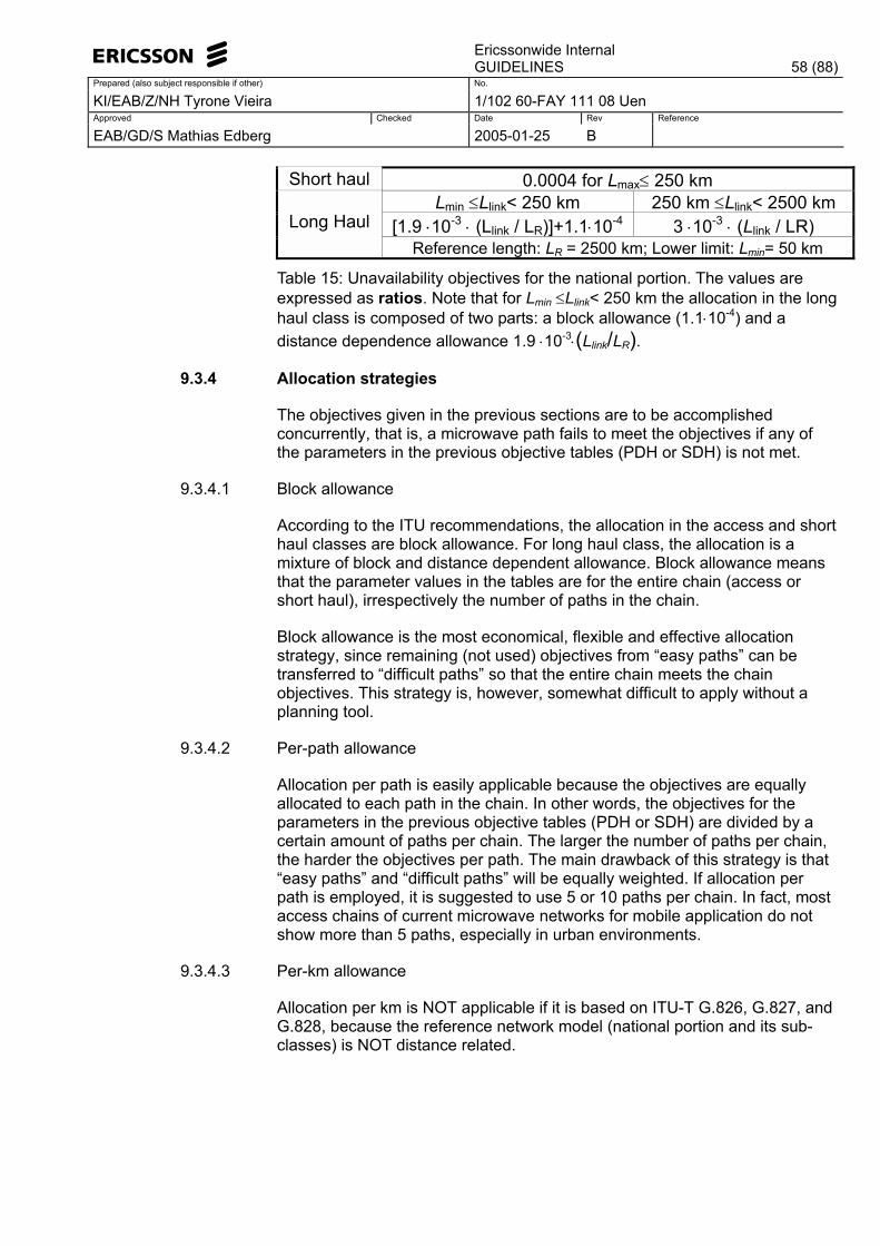
Ericssonwide Internal
GUIDELINES 58 (88)Prepared (also subject responsible if other) No.
KI/EAB/Z/NH Tyrone Vieira 1/102 60-FAY 111 08 Uen Approved Checked Date Rev Reference
EAB/GD/S Mathias Edberg 2005-01-25 B
Short haul 0.0004 for Lmax≤ 250 km Lmin ≤Llink< 250 km 250 km ≤Llink< 2500 km
[1.9 ⋅10-3 ⋅ (Llink / LR)]+1.1⋅10-4 3 ⋅10-3 ⋅ (Llink / LR)
Long Haul Reference length: LR = 2500 km; Lower limit: Lmin= 50 km
Table 15: Unavailability objectives for the national portion. The values are expressed as ratios. Note that for Lmin ≤Llink< 250 km the allocation in the long haul class is composed of two parts: a block allowance (1.1⋅10-4) and a distance dependence allowance 1.9 ⋅10-3⋅(Llink/LR).
9.3.4 Allocation strategies
The objectives given in the previous sections are to be accomplished concurrently, that is, a microwave path fails to meet the objectives if any of the parameters in the previous objective tables (PDH or SDH) is not met.
9.3.4.1 Block allowance
According to the ITU recommendations, the allocation in the access and short haul classes are block allowance. For long haul class, the allocation is a mixture of block and distance dependent allowance. Block allowance means that the parameter values in the tables are for the entire chain (access or short haul), irrespectively the number of paths in the chain.
Block allowance is the most economical, flexible and effective allocation strategy, since remaining (not used) objectives from �easy paths� can be transferred to �difficult paths� so that the entire chain meets the chain objectives. This strategy is, however, somewhat difficult to apply without a planning tool.
9.3.4.2 Per-path allowance
Allocation per path is easily applicable because the objectives are equally allocated to each path in the chain. In other words, the objectives for the parameters in the previous objective tables (PDH or SDH) are divided by a certain amount of paths per chain. The larger the number of paths per chain, the harder the objectives per path. The main drawback of this strategy is that �easy paths� and �difficult paths� will be equally weighted. If allocation per path is employed, it is suggested to use 5 or 10 paths per chain. In fact, most access chains of current microwave networks for mobile application do not show more than 5 paths, especially in urban environments.
9.3.4.3 Per-km allowance
Allocation per km is NOT applicable if it is based on ITU-T G.826, G.827, and G.828, because the reference network model (national portion and its sub-classes) is NOT distance related.
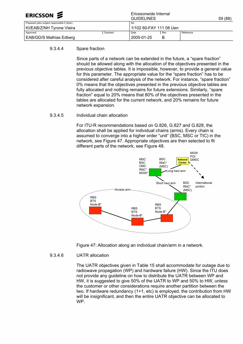
Ericssonwide Internal
GUIDELINES 59 (88)Prepared (also subject responsible if other) No.
KI/EAB/Z/NH Tyrone Vieira 1/102 60-FAY 111 08 Uen Approved Checked Date Rev Reference
EAB/GD/S Mathias Edberg 2005-01-25 B
9.3.4.4 Spare fraction
Since parts of a network can be extended in the future, a �spare fraction� should be allowed along with the allocation of the objectives presented in the previous objective tables. It is impossible, however, to provide a general value for this parameter. The appropriate value for the �spare fraction� has to be considered after careful analysis of the network. For instance, �spare fraction� 0% means that the objectives presented in the previous objective tables are fully allocated and nothing remains for future extensions. Similarly, �spare fraction� equal to 20% means that 80% of the objectives presented in the tables are allocated for the current network, and 20% remains for future network expansion.
9.3.4.5 Individual chain allocation
For ITU-R recommendations based on G.826, G.827 and G.828, the allocation shall be applied for individual chains (arms). Every chain is assumed to converge into a higher order �unit� (BSC, MSC or TIC) in the network, see Figure 47. Appropriate objectives are then selected to fit different parts of the network, see Figure 48.
RBSBTSNode-B*
BSCRNC*(MSC)
RBSBTSNode-B*
RBSBTSNode-B*
Access arm
BSCRNC*(MSC)
BSC
RNC*OMC
MSC
MGW*
Short haul arm
MGWPOIGMSCNational
Center
Long haul arm
Internationalportion
Figure 47: Allocation along an individual chain/arm in a network.
9.3.4.6 UATR allocation
The UATR objectives given in Table 15 shall accommodate for outage due to radiowave propagation (WP) and hardware failure (HW). Since the ITU does not provide any guideline on how to distribute the UATR between WP and HW, it is suggested to give 50% of the UATR to WP and 50% to HW, unless the customer or other considerations require another partition between the two. If hardware redundancy (1+1, etc) is employed, the contribution from HW will be insignificant, and then the entire UATR objective can be allocated to WP.
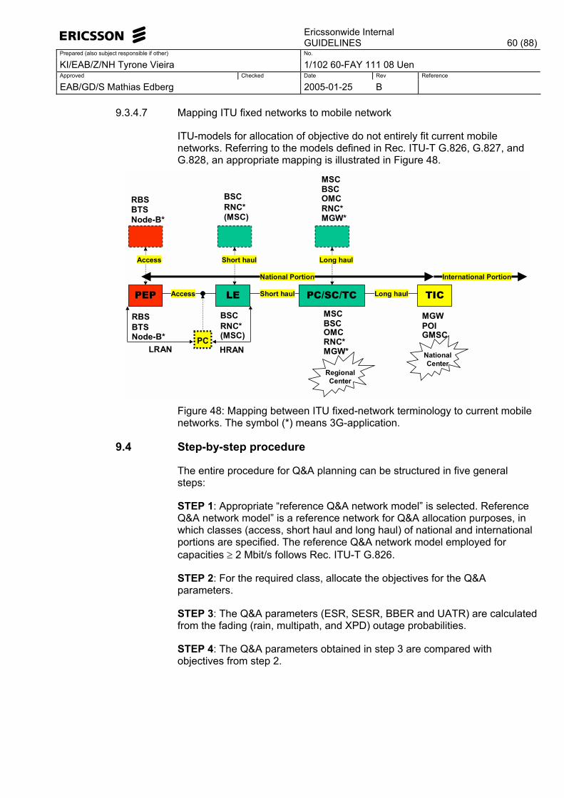
Ericssonwide Internal
GUIDELINES 60 (88)Prepared (also subject responsible if other) No.
KI/EAB/Z/NH Tyrone Vieira 1/102 60-FAY 111 08 Uen Approved Checked Date Rev Reference
EAB/GD/S Mathias Edberg 2005-01-25 B
9.3.4.7 Mapping ITU fixed networks to mobile network
ITU-models for allocation of objective do not entirely fit current mobile networks. Referring to the models defined in Rec. ITU-T G.826, G.827, and G.828, an appropriate mapping is illustrated in Figure 48.
PEP
RBSBTSNode-B*
LE PC/SC/TC TIC
BSCRNC* BSC
RNC*
Access Short haul Long haul
OMC
RBSBTSNode-B*
Access Short haul Long haul
PC
National Portion International Portion
(MSC)
MSC
MGW*
MGWPOIGMSC
BSCRNC*(MSC)
BSC
RNC*OMC
MSC
MGW*
NationalCenter
RegionalCenter
HRANLRAN
Figure 48: Mapping between ITU fixed-network terminology to current mobile networks. The symbol (*) means 3G-application.
9.4 Step-by-step procedure
The entire procedure for Q&A planning can be structured in five general steps:
STEP 1: Appropriate �reference Q&A network model� is selected. Reference Q&A network model� is a reference network for Q&A allocation purposes, in which classes (access, short haul and long haul) of national and international portions are specified. The reference Q&A network model employed for capacities ≥ 2 Mbit/s follows Rec. ITU-T G.826.
STEP 2: For the required class, allocate the objectives for the Q&A parameters.
STEP 3: The Q&A parameters (ESR, SESR, BBER and UATR) are calculated from the fading (rain, multipath, and XPD) outage probabilities.
STEP 4: The Q&A parameters obtained in step 3 are compared with objectives from step 2.
Ericssonwide Internal
GUIDELINES 61 (88)Prepared (also subject responsible if other) No.
KI/EAB/Z/NH Tyrone Vieira 1/102 60-FAY 111 08 Uen Approved Checked Date Rev Reference
EAB/GD/S Mathias Edberg 2005-01-25 B
STEP 5: If the objectives are not met, then appropriate network parameters (antenna size, antenna height, output power, channel arrangements, polarization, etc) are changed and the quality and availability parameters are re-calculated as described in step 3. The procedure is continued through step 4 as an iterative process until the calculated Q&A parameters met the objectives for the Q&A parameters.
9.5 Planning advices • Multipath (flat and frequency selective) and XPD outages give ESR,
SESR and BBER. • Rain and XPD outages give UATR. • Quality is normally the dimensioning aspect for �lower� frequencies
(roughly lower than 13 GHz) while unavailability is normally the dimensioning aspect for �higher� frequencies (roughly higher than 13 GHz). In the range 13 to 18 GHz, planning for extreme scenarios (large paths in rain or multipath rich regions) may force quality or unavailability as dimensioning.
• The objectives shall account for effects caused by fading, interference and other sources of performance degradation.
• The objectives are to be met over an evaluation period of 30 consecutive days.
• The objectives are applicable independently to each direction of transmission.
• SDH-paths meeting the objective allocation described above will enable the ATM traffic to meet the requirements in ITU-T Rec. I.356.
• It has been found that ESR is rarely or never dimensioning. • BBER is only dimensioning for low fade margins (for instance using lower
output powers and small antennas) • SESR is in most applications the only quality dimensioning parameter. • ITU-T G.828-based objectives are harder than ITU-T G.826 for ESR and
BBER, but equal for SESR and UATR. Since BBER and ESR are rarely or never dimensioning, the dimensioning properties given by the SESR and UATR objectives are quite often independent whether ITU-T G.828 or G.826 is employed.
• Distance-based allocation (%/km) in the access and short haul is not supported by any ITU-R recommendation based on Rec. ITU-T G.826, G.827 and G.828 (the portions of the network model are not length-defined�).
• Distance-based allocation distributes the objectives equally along a radio link (chain of paths). This is not effective since �difficult paths� normally require more objective apportionment than �easy paths�.
• Unavailability due to hardware failure is not length-related while unavailability due to radiowave propagation (rain and refraction-diffraction fading) can be strongly length dependent. The contribution from hardware failure in path chains having many short hops becomes too high, then making allocation very difficult.
• Networks that are better than good are a waste of money!

Ericssonwide Internal
GUIDELINES 62 (88)Prepared (also subject responsible if other) No.
KI/EAB/Z/NH Tyrone Vieira 1/102 60-FAY 111 08 Uen Approved Checked Date Rev Reference
EAB/GD/S Mathias Edberg 2005-01-25 B
9.6 TEMS LinkPlanner application
Three basic tables should always be available in TEMS LinkPlanner: based on Rec. ITU-T G.821 (for capacity lower than 2 Mbit/s), based on ITU-T G.826 (for PDH-links with capacity higher than 2 Mbit/s), and based on ITU-T G.828 (for SDH-links). Rec. ITU-T G.827 is the base for UATR and entered in the last column of the latter two tables. Figure 49 shows table for objectives based on Rec. ITU-T G.826 (ESR, SESR and BBER) and Rec. ITU-T G.827 (UATR). Note, however, that the objectives are defined by ITU-R recommendations but based on ITU-T recommendations.
Figure 49: Defining a table for objectives based on Rec. ITU-T G.826 (ESR, SESR and BBER) for the access portion of the HRP and Rec. ITU-T G.827 (UATR).
10 Planning procedures
The planning procedures provided in this section are for Remote Transmit Power Control (RTPC). For Automatic Transmit Power Control (ATPC) the reader is referred to the planning rules given in [11].
10.1 Design overview
Depending on customer requirements, special agreements on delivery, economical aspects, and the degree of involvement of Ericsson, the design of a microwave network can be carried out in many different ways. In what follows, an overview of commonly design phases is presented.
If a completely new microwave network is to be designed, then geographical, demographical and economical information is of great importance to select site candidates. Unfortunately, when transmission planning is requested the sites are normally already selected and acquired. Sites having good geographical/strategic location as well developed infrastructures are attractive and consequently resulting in geographically co-location of several services and operators.
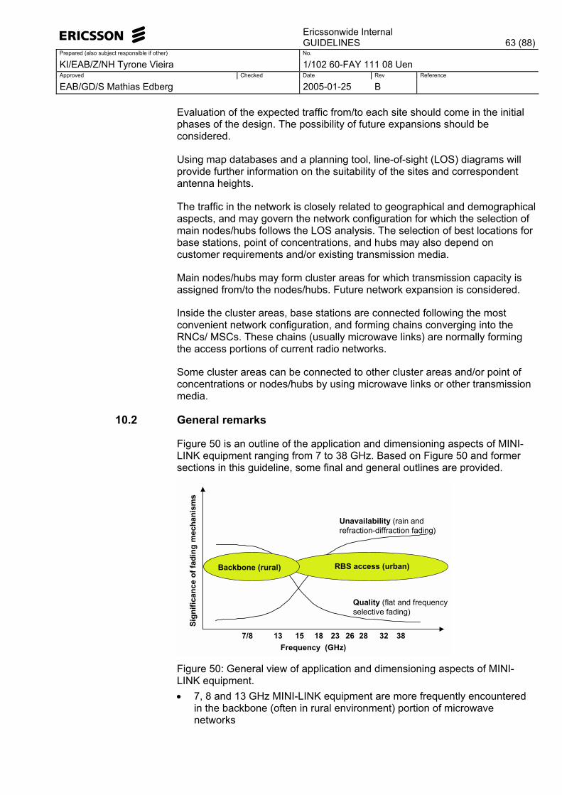
Ericssonwide Internal
GUIDELINES 63 (88)Prepared (also subject responsible if other) No.
KI/EAB/Z/NH Tyrone Vieira 1/102 60-FAY 111 08 Uen Approved Checked Date Rev Reference
EAB/GD/S Mathias Edberg 2005-01-25 B
Evaluation of the expected traffic from/to each site should come in the initial phases of the design. The possibility of future expansions should be considered.
Using map databases and a planning tool, line-of-sight (LOS) diagrams will provide further information on the suitability of the sites and correspondent antenna heights.
The traffic in the network is closely related to geographical and demographical aspects, and may govern the network configuration for which the selection of main nodes/hubs follows the LOS analysis. The selection of best locations for base stations, point of concentrations, and hubs may also depend on customer requirements and/or existing transmission media.
Main nodes/hubs may form cluster areas for which transmission capacity is assigned from/to the nodes/hubs. Future network expansion is considered.
Inside the cluster areas, base stations are connected following the most convenient network configuration, and forming chains converging into the RNCs/ MSCs. These chains (usually microwave links) are normally forming the access portions of current radio networks.
Some cluster areas can be connected to other cluster areas and/or point of concentrations or nodes/hubs by using microwave links or other transmission media.
10.2 General remarks
Figure 50 is an outline of the application and dimensioning aspects of MINI-LINK equipment ranging from 7 to 38 GHz. Based on Figure 50 and former sections in this guideline, some final and general outlines are provided.
13Frequency (GHz)
Unavailability (rain and refraction-diffraction fading)
Quality (flat and frequency selective fading)
RBS access (urban)Backbone (rural)
Sign
ifica
nce
of fa
ding
mec
hani
sms
7/8 15 18 2623 28 3832
Figure 50: General view of application and dimensioning aspects of MINI-LINK equipment. • 7, 8 and 13 GHz MINI-LINK equipment are more frequently encountered
in the backbone (often in rural environment) portion of microwave networks
Ericssonwide Internal
GUIDELINES 64 (88)Prepared (also subject responsible if other) No.
KI/EAB/Z/NH Tyrone Vieira 1/102 60-FAY 111 08 Uen Approved Checked Date Rev Reference
EAB/GD/S Mathias Edberg 2005-01-25 B
• MINI-LINK equipment ranging from 15 GHz to 38 GHz is more frequently encountered connecting RBS in the access (normally in urban environment) portion of microwave networks.
• Four fading mechanisms are currently involved in outage calculations: rain, refraction-diffraction, multipath flat, and multipath selective.
• Since rain and refraction-diffraction fading are characterized by slow event occurrences (normally lasting for more than 10 consecutive seconds), unavailability (UATR) is the main contribution.
• Since multipath flat and frequency selective fading are characterized by very fast event occurrences (normally lasting shorter than 10 consecutive seconds), quality (ESR, SESR and BBER) is the main contribution.
• The dimensioning aspect for 7/8 GHz and often even 13 GHz MINI-LINK equipment is normally the quality.
• The dimensioning aspect for MINI-LINK equipment ranging from 15 GHz to 38 GHz is normally unavailability.
• The frequencies 13, 15 and 18 GHz are located in a somewhat grey frequency region, in which both unavailability and/or quality can be the dimensioning aspects due to unreasonable path lengths in extreme propagation conditions. Theoretically, it is possible that unusual long paths in rain-rich regions may force unavailability to be the dimensioning aspect even for frequencies as low as 7/8 GHz. Similarly, unusual long paths in difficult atmospheric layers force the quality to be the dimensioning aspect even for frequencies higher than 18 GHz where normally the unavailability is dominating.
• PDH-links shall be planned employing ITU-R objectives based on Rec. ITU-T G.826 (quality) and Rec. ITU-T G.827 (unavailability).
• SDH-links shall be planned employing ITU-R objectives based on Rec. ITU-T G.828 (quality) and Rec. ITU-T G.827 (unavailability).
• It has been demonstrated elsewhere that the parameter ESR is never dimensioning whatever the used MINI-LINK configuration.
• SESR is normally the dimensioning quality parameter. • BBER might be the dimensioning quality parameter if smaller antennas
are used in combination with low output power for such paths where the fade margin is too low.
• UATR should always accommodate unavailability due to hardware failure (HW) and radiowave (RW) propagation effects. For protected MINI-LINK configurations, however, the HW contribution to unavailability is almost insignificant, and therefore the UATR objective can be entirely allocated to account for propagation effects.
• Microwave networks can be expanded in the future. This can be considered by not using the entire quality and availability objectives. A kind of �spare fraction� can be left for future expansions, but its value (10%, 20% or 30%) is not a general rule and should therefore be discussed from case to case.
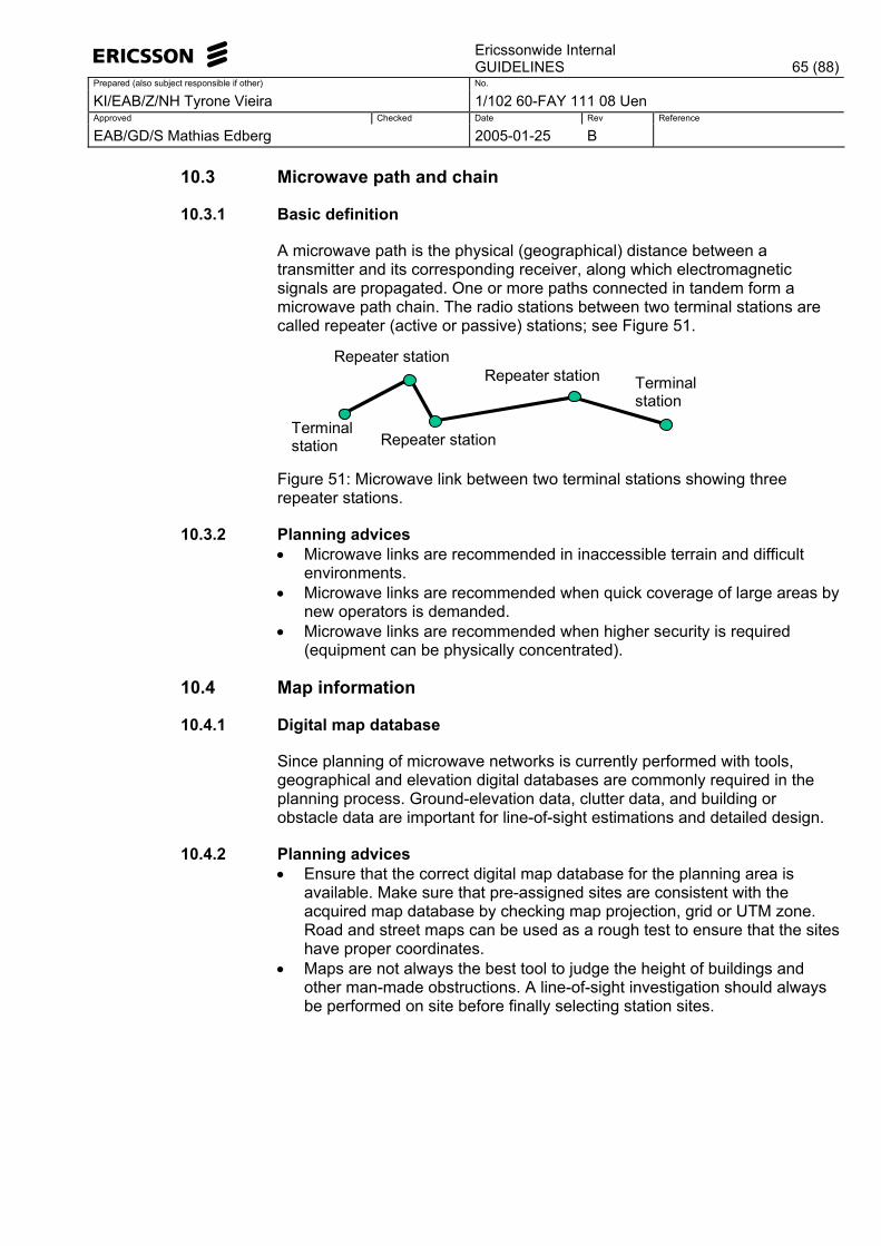
Ericssonwide Internal
GUIDELINES 65 (88)Prepared (also subject responsible if other) No.
KI/EAB/Z/NH Tyrone Vieira 1/102 60-FAY 111 08 Uen Approved Checked Date Rev Reference
EAB/GD/S Mathias Edberg 2005-01-25 B
10.3 Microwave path and chain
10.3.1 Basic definition
A microwave path is the physical (geographical) distance between a transmitter and its corresponding receiver, along which electromagnetic signals are propagated. One or more paths connected in tandem form a microwave path chain. The radio stations between two terminal stations are called repeater (active or passive) stations; see Figure 51.
Repeater station
Repeater station
Repeater station Terminal station
Terminal station
Figure 51: Microwave link between two terminal stations showing three repeater stations.
10.3.2 Planning advices • Microwave links are recommended in inaccessible terrain and difficult
environments. • Microwave links are recommended when quick coverage of large areas by
new operators is demanded. • Microwave links are recommended when higher security is required
(equipment can be physically concentrated).
10.4 Map information
10.4.1 Digital map database
Since planning of microwave networks is currently performed with tools, geographical and elevation digital databases are commonly required in the planning process. Ground-elevation data, clutter data, and building or obstacle data are important for line-of-sight estimations and detailed design.
10.4.2 Planning advices • Ensure that the correct digital map database for the planning area is
available. Make sure that pre-assigned sites are consistent with the acquired map database by checking map projection, grid or UTM zone. Road and street maps can be used as a rough test to ensure that the sites have proper coordinates.
• Maps are not always the best tool to judge the height of buildings and other man-made obstructions. A line-of-sight investigation should always be performed on site before finally selecting station sites.
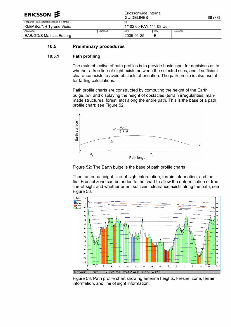
Ericssonwide Internal
GUIDELINES 66 (88)Prepared (also subject responsible if other) No.
KI/EAB/Z/NH Tyrone Vieira 1/102 60-FAY 111 08 Uen Approved Checked Date Rev Reference
EAB/GD/S Mathias Edberg 2005-01-25 B
10.5 Preliminary procedures
10.5.1 Path profiling
The main objective of path profiles is to provide basic input for decisions as to whether a free line-of-sight exists between the selected sites, and if sufficient clearance exists to avoid obstacle attenuation. The path profile is also useful for fading calculations.
Path profile charts are constructed by computing the height of the Earth bulge, ∆h, and displaying the height of obstacles (terrain irregularities, man-made structures, forest, etc) along the entire path. This is the base of a path profile chart; see Figure 52.
d2
d1
∆h
Path length
Earth
sur
face
Rkddh⋅⋅
⋅=∆
221
Figure 52: The Earth bulge is the base of path profile charts
Then, antenna height, line-of-sight information, terrain information, and the first Fresnel zone can be added to the chart to allow the determination of free line-of-sight and whether or not sufficient clearance exists along the path, see Figure 53.
Figure 53: Path profile chart showing antenna heights, Fresnel zone, terrain information, and line of sight information.
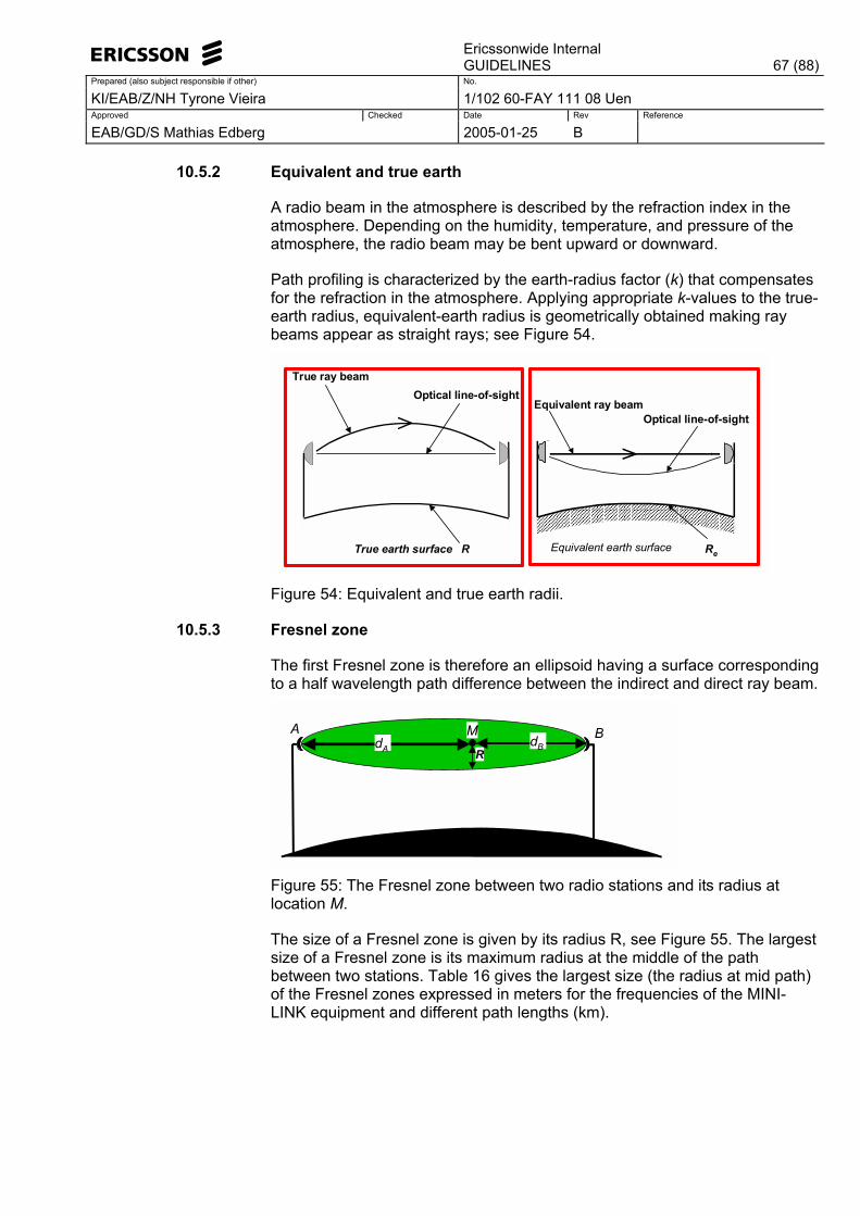
Ericssonwide Internal
GUIDELINES 67 (88)Prepared (also subject responsible if other) No.
KI/EAB/Z/NH Tyrone Vieira 1/102 60-FAY 111 08 Uen Approved Checked Date Rev Reference
EAB/GD/S Mathias Edberg 2005-01-25 B
10.5.2 Equivalent and true earth
A radio beam in the atmosphere is described by the refraction index in the atmosphere. Depending on the humidity, temperature, and pressure of the atmosphere, the radio beam may be bent upward or downward.
Path profiling is characterized by the earth-radius factor (k) that compensates for the refraction in the atmosphere. Applying appropriate k-values to the true-earth radius, equivalent-earth radius is geometrically obtained making ray beams appear as straight rays; see Figure 54.
True earth surface
Optical line-of-sightTrue ray beam
R
Equivalent ray beam
Equivalent earth surface
Optical line-of-sight
Re
Figure 54: Equivalent and true earth radii.
10.5.3 Fresnel zone
The first Fresnel zone is therefore an ellipsoid having a surface corresponding to a half wavelength path difference between the indirect and direct ray beam.
MA BR
dBdA
Figure 55: The Fresnel zone between two radio stations and its radius at location M.
The size of a Fresnel zone is given by its radius R, see Figure 55. The largest size of a Fresnel zone is its maximum radius at the middle of the path between two stations. Table 16 gives the largest size (the radius at mid path) of the Fresnel zones expressed in meters for the frequencies of the MINI-LINK equipment and different path lengths (km).
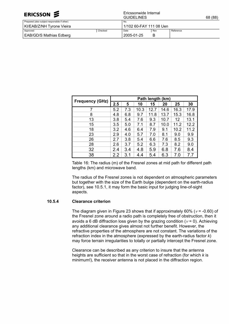
Ericssonwide Internal
GUIDELINES 68 (88)Prepared (also subject responsible if other) No.
KI/EAB/Z/NH Tyrone Vieira 1/102 60-FAY 111 08 Uen Approved Checked Date Rev Reference
EAB/GD/S Mathias Edberg 2005-01-25 B
Path length (km) Frequency (GHz)
2.5 5 10 15 20 25 30 7 5.2 7.3 10.3 12.7 14.6 16.3 17.9 8 4.8 6.8 9.7 11.8 13.7 15.3 16.8
13 3.8 5.4 7.6 9.3 10.7 12 13.1 15 3.5 5.0 7.1 8.7 10.0 11.2 12.2 18 3.2 4.6 6.4 7.9 9.1 10.2 11.2 23 2.9 4.0 5.7 7.0 8.1 9.0 9.9 26 2.7 3.8 5.4 6.6 7.6 8.5 9.3 28 2.6 3.7 5.2 6.3 7.3 8.2 9.0 32 2.4 3.4 4.8 5.9 6.8 7.6 8.4 38 2.2 3.1 4.4 5.4 6.3 7.0 7.7
Table 16: The radius (m) of the Fresnel zones at mid path for different path lengths (km) and microwave band.
The radius of the Fresnel zones is not dependent on atmospheric parameters but together with the size of the Earth bulge (dependent on the earth-radius factor), see 10.5.1, it may form the basic input for judging line-of-sight aspects.
10.5.4 Clearance criterion
The diagram given in Figure 23 shows that if approximately 60% (ν = -0.60) of the Fresnel zone around a radio path is completely free of obstruction, then it avoids a 6 dB diffraction loss given by the grazing condition (ν = 0). Achieving any additional clearance gives almost not further benefit. However, the refractive properties of the atmosphere are not constant. The variations of the refraction index in the atmosphere (expressed by the earth-radius factor k) may force terrain irregularities to totally or partially intercept the Fresnel zone.
Clearance can be described as any criterion to insure that the antenna heights are sufficient so that in the worst case of refraction (for which k is minimum!), the receiver antenna is not placed in the diffraction region.
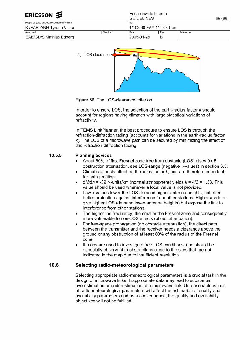
Ericssonwide Internal
GUIDELINES 69 (88)Prepared (also subject responsible if other) No.
KI/EAB/Z/NH Tyrone Vieira 1/102 60-FAY 111 08 Uen Approved Checked Date Rev Reference
EAB/GD/S Mathias Edberg 2005-01-25 B
hChC= LOS-clearance
Figure 56: The LOS-clearance criterion.
In order to ensure LOS, the selection of the earth-radius factor k should account for regions having climates with large statistical variations of refractivity.
In TEMS LinkPlanner, the best procedure to ensure LOS is through the refraction-diffraction fading (accounts for variations in the earth-radius factor k). The LOS of a microwave path can be secured by minimizing the effect of this refraction-diffraction fading.
10.5.5 Planning advices • About 60% of first Fresnel zone free from obstacle (LOS) gives 0 dB
obstruction attenuation, see LOS-range (negative ν-values) in section 6.5. • Climatic aspects affect earth-radius factor k, and are therefore important
for path profiling. • dN/dh = -39 N-units/km (normal atmosphere) yields k = 4/3 = 1.33. This
value should be used whenever a local value is not provided. • Low k-values lower the LOS demand higher antenna heights, but offer
better protection against interference from other stations. Higher k-values give higher LOS (demand lower antenna heights) but expose the link to interference from other stations.
• The higher the frequency, the smaller the Fresnel zone and consequently more vulnerable to non-LOS effects (object attenuation).
• For free-space propagation (no obstacle attenuation), the direct path between the transmitter and the receiver needs a clearance above the ground or any obstruction of at least 60% of the radius of the Fresnel zone.
• If maps are used to investigate free LOS conditions, one should be especially observant to obstructions close to the sites that are not indicated in the map due to insufficient resolution.
10.6 Selecting radio-meteorological parameters
Selecting appropriate radio-meteorological parameters is a crucial task in the design of microwave links. Inappropriate data may lead to substantial overestimation or underestimation of a microwave link. Unreasonable values of radio-meteorological parameters will affect the estimation of quality and availability parameters and as a consequence, the quality and availability objectives will not be fulfilled.
Ericssonwide Internal
GUIDELINES 70 (88)Prepared (also subject responsible if other) No.
KI/EAB/Z/NH Tyrone Vieira 1/102 60-FAY 111 08 Uen Approved Checked Date Rev Reference
EAB/GD/S Mathias Edberg 2005-01-25 B
Chapter 15 of [10] gives a detailed presentation on the selection of radio-meteorological parameters.
10.6.1 Earth-radius factor (k)
Application: used for path profiling, derivation of LOS, and indirectly important for interference aspects.
Planning aspects: 1) Low k-values lower the LOS (demand higher antenna heights) but offer better protection against interference from other stations. Higher k-values give higher LOS (demand lower antenna heights) but expose the link to interference from other stations. 2) The k-value for a normal atmosphere (k=1.33) should be used whenever local k-value is not provided. 3) The earth-radius factor k can be obtained in the following way: A) select the appropriate value of the refractivity gradient (∆N); see next section. B) The k-value is given by k = 157/(157 + ∆N).
Use in planning tools: In TEMS LinkPlanner the k-value is automatically derived from pL-distributions (see below)
10.6.2 Refractivity gradient
Application: used to determine the k-value and therefore it governs path profiling, derivation of LOS, as well as it is indirectly important for interference aspects. Also employed in ray tracing calculations. The refractivity gradient for normal propagation conditions is dN/dh=-40 N-units/km. It is negative because the refractivity (via temperature, atmospheric pressure and humidity) decreases when the antenna height increases.
Planning aspects: 1) for any specific geographical region, select the highest value if lower LOS is required, 2) for any specific geographical region, select the lowest value if higher LOS is required.
Use in planning tools: Since k-value is automatically derived from pL-distributions in TEMS LinkPlanner, this parameter is not entered.
10.6.3 Point refractivity gradient
Application: used for flat fading calculations. It is a new parameter defined by the ITU-R as the refractivity gradient in the lowest 65 m of the atmosphere not exceeded for 1% of an average year. Its average value depends very much on the elevation of terrain.
Planning aspects: High values of the point refractivity gradient symbolize intensive multipath activities in the atmosphere since this variable provide a measure of the extreme ducts or ducting conditions in the ground.
Use in planning tools: The point refractivity gradient is manually entered in TEMS LinkPlanner.
Ericssonwide Internal
GUIDELINES 71 (88)Prepared (also subject responsible if other) No.
KI/EAB/Z/NH Tyrone Vieira 1/102 60-FAY 111 08 Uen Approved Checked Date Rev Reference
EAB/GD/S Mathias Edberg 2005-01-25 B
10.6.4 Refractivity factor � pL-factor
Application: used for flat fading calculations. It is the old parameter in the former flat fading model and defined by the ITU-R as the percentage of time that the refractivity gradient in the lowest 100 m of the atmosphere is more negative than -100 N units/km in the estimated average worst month.
Planning aspects: 1) High pL-values symbolize intensive multipath activities in the atmosphere. 2) Due to the seasonal dependence of the pL-factor, select seasonal chart that gives the highest pL-value.
Use in planning tools: In TEMS LinkPlanner the pL-factor is entered manually.
10.6.5 Surface water vapor density
Application: used for calculation of water vapor attenuation in the atmosphere. Varies from 1 to 25 g/m3.
Planning aspects: 1) high density values symbolize high humidity in the atmosphere, 2) due to the seasonal dependence of the surface water vapor density, select seasonal chart that gives the highest density value.
Use in planning tools: Replaced in TEMS LinkPlanner by relative humidity and temperature, see bellow.
10.6.6 Temperature
Application: together with relative humidity, it is used for calculation of water vapor attenuation in the atmosphere.
Planning aspects: 1) Higher temperature gives higher saturation pressure and consequently higher humidity, that is, more water vapor attenuation. 2) Large geographical regions located in the tropic zone and island conglomeration show minor variations from the annual mean given in the chart. Examples are the Caribbean, Canaries, and Micronesia islands. 3) For other regions, a reasonable approach is to select the local mean temperature in the summer. High temperature gives high attenuation.
Use in planning tools: In TEMS LinkPlanner the temperature is entered manually.
10.6.7 Relative humidity
Application: together with temperature, it is used for calculation of water vapor attenuation in the atmosphere.
Planning aspects: 1) Relative humidity is not a good indicator of the real water content in the atmosphere. High values of relative humidity do not automatically imply high humidity in the atmosphere if the temperature is low. 2) Lower values of relative humidity along with higher values of temperature may give high humidity (more water content, more attenuation).
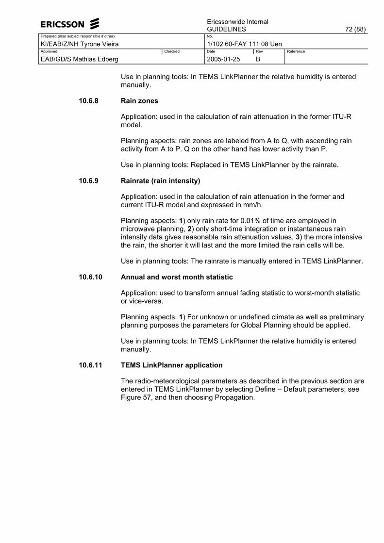
Ericssonwide Internal
GUIDELINES 72 (88)Prepared (also subject responsible if other) No.
KI/EAB/Z/NH Tyrone Vieira 1/102 60-FAY 111 08 Uen Approved Checked Date Rev Reference
EAB/GD/S Mathias Edberg 2005-01-25 B
Use in planning tools: In TEMS LinkPlanner the relative humidity is entered manually.
10.6.8 Rain zones
Application: used in the calculation of rain attenuation in the former ITU-R model.
Planning aspects: rain zones are labeled from A to Q, with ascending rain activity from A to P. Q on the other hand has lower activity than P.
Use in planning tools: Replaced in TEMS LinkPlanner by the rainrate.
10.6.9 Rainrate (rain intensity)
Application: used in the calculation of rain attenuation in the former and current ITU-R model and expressed in mm/h.
Planning aspects: 1) only rain rate for 0.01% of time are employed in microwave planning, 2) only short-time integration or instantaneous rain intensity data gives reasonable rain attenuation values, 3) the more intensive the rain, the shorter it will last and the more limited the rain cells will be.
Use in planning tools: The rainrate is manually entered in TEMS LinkPlanner.
10.6.10 Annual and worst month statistic
Application: used to transform annual fading statistic to worst-month statistic or vice-versa.
Planning aspects: 1) For unknown or undefined climate as well as preliminary planning purposes the parameters for Global Planning should be applied.
Use in planning tools: In TEMS LinkPlanner the relative humidity is entered manually.
10.6.11 TEMS LinkPlanner application
The radio-meteorological parameters as described in the previous section are entered in TEMS LinkPlanner by selecting Define � Default parameters; see Figure 57, and then choosing Propagation.
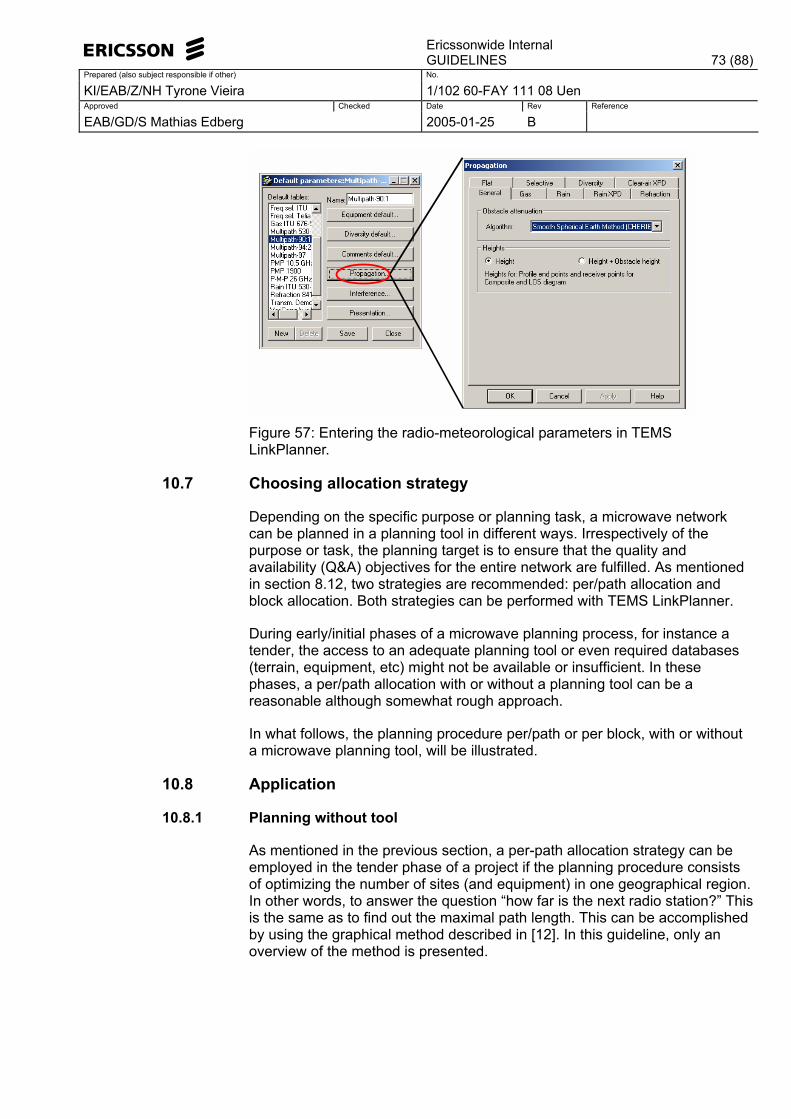
Ericssonwide Internal
GUIDELINES 73 (88)Prepared (also subject responsible if other) No.
KI/EAB/Z/NH Tyrone Vieira 1/102 60-FAY 111 08 Uen Approved Checked Date Rev Reference
EAB/GD/S Mathias Edberg 2005-01-25 B
Figure 57: Entering the radio-meteorological parameters in TEMS LinkPlanner.
10.7 Choosing allocation strategy
Depending on the specific purpose or planning task, a microwave network can be planned in a planning tool in different ways. Irrespectively of the purpose or task, the planning target is to ensure that the quality and availability (Q&A) objectives for the entire network are fulfilled. As mentioned in section 8.12, two strategies are recommended: per/path allocation and block allocation. Both strategies can be performed with TEMS LinkPlanner.
During early/initial phases of a microwave planning process, for instance a tender, the access to an adequate planning tool or even required databases (terrain, equipment, etc) might not be available or insufficient. In these phases, a per/path allocation with or without a planning tool can be a reasonable although somewhat rough approach.
In what follows, the planning procedure per/path or per block, with or without a microwave planning tool, will be illustrated.
10.8 Application
10.8.1 Planning without tool
As mentioned in the previous section, a per-path allocation strategy can be employed in the tender phase of a project if the planning procedure consists of optimizing the number of sites (and equipment) in one geographical region. In other words, to answer the question �how far is the next radio station?� This is the same as to find out the maximal path length. This can be accomplished by using the graphical method described in [12]. In this guideline, only an overview of the method is presented.
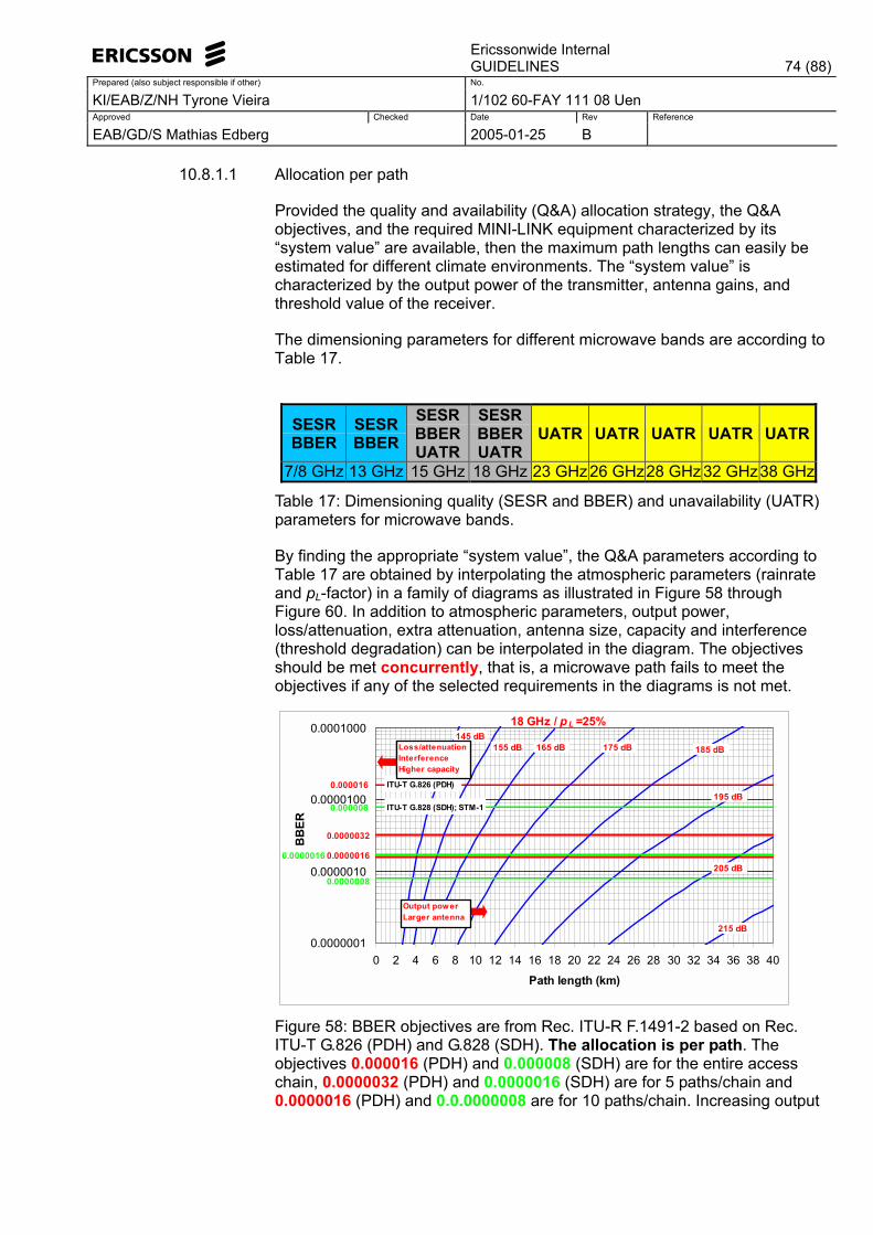
Ericssonwide Internal
GUIDELINES 74 (88)Prepared (also subject responsible if other) No.
KI/EAB/Z/NH Tyrone Vieira 1/102 60-FAY 111 08 Uen Approved Checked Date Rev Reference
EAB/GD/S Mathias Edberg 2005-01-25 B
10.8.1.1 Allocation per path
Provided the quality and availability (Q&A) allocation strategy, the Q&A objectives, and the required MINI-LINK equipment characterized by its �system value� are available, then the maximum path lengths can easily be estimated for different climate environments. The �system value� is characterized by the output power of the transmitter, antenna gains, and threshold value of the receiver.
The dimensioning parameters for different microwave bands are according to Table 17.
SESR BBER
SESRBBER
SESRBBERUATR
SESRBBERUATR
UATR UATR UATR UATR UATR
7/8 GHz 13 GHz 15 GHz 18 GHz 23 GHz26 GHz 28 GHz 32 GHz38 GHz
Table 17: Dimensioning quality (SESR and BBER) and unavailability (UATR) parameters for microwave bands.
By finding the appropriate �system value�, the Q&A parameters according to Table 17 are obtained by interpolating the atmospheric parameters (rainrate and pL-factor) in a family of diagrams as illustrated in Figure 58 through Figure 60. In addition to atmospheric parameters, output power, loss/attenuation, extra attenuation, antenna size, capacity and interference (threshold degradation) can be interpolated in the diagram. The objectives should be met concurrently, that is, a microwave path fails to meet the objectives if any of the selected requirements in the diagrams is not met.
0.0000001
0.0000010
0.0000100
0.0001000
0 2 4 6 8 10 12 14 16 18 20 22 24 26 28 30 32 34 36 38 40
Path length (km)
BB
ER
18 GHz / p L =25%
ITU-T G.826 (PDH)
ITU-T G.828 (SDH); STM-1
0.000016
0.0000032
0.0000016
0.000008
0.0000016
0.0000008
145 dB155 dB 165 dB 175 dB
Output powerLarger antenna
Loss/attenuationInterferenceHigher capacity
185 dB
195 dB
205 dB
215 dB
Figure 58: BBER objectives are from Rec. ITU-R F.1491-2 based on Rec. ITU-T G.826 (PDH) and G.828 (SDH). The allocation is per path. The objectives 0.000016 (PDH) and 0.000008 (SDH) are for the entire access chain, 0.0000032 (PDH) and 0.0000016 (SDH) are for 5 paths/chain and 0.0000016 (PDH) and 0.0.0000008 are for 10 paths/chain. Increasing output
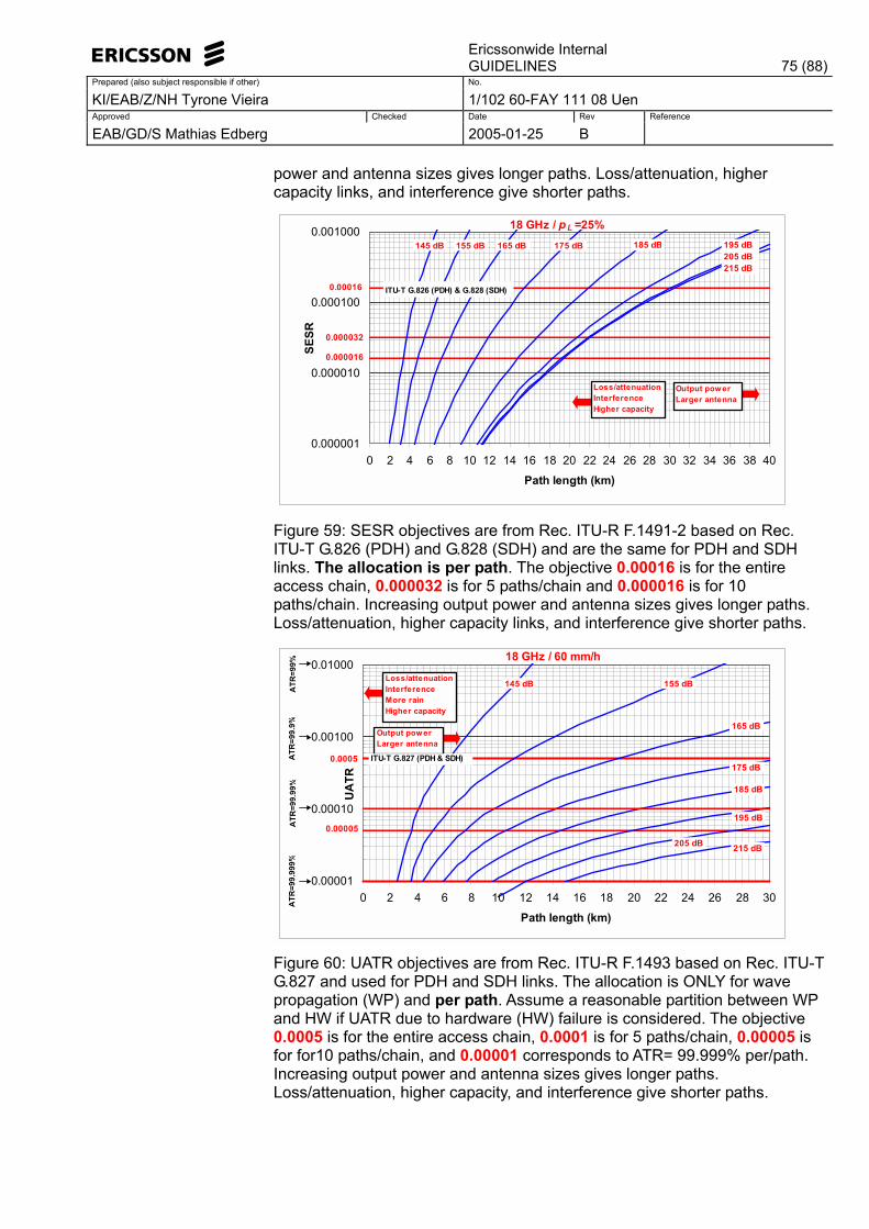
Ericssonwide Internal
GUIDELINES 75 (88)Prepared (also subject responsible if other) No.
KI/EAB/Z/NH Tyrone Vieira 1/102 60-FAY 111 08 Uen Approved Checked Date Rev Reference
EAB/GD/S Mathias Edberg 2005-01-25 B
power and antenna sizes gives longer paths. Loss/attenuation, higher capacity links, and interference give shorter paths.
0.000001
0.000010
0.000100
0.001000
0 2 4 6 8 10 12 14 16 18 20 22 24 26 28 30 32 34 36 38 40
Path length (km)
SESR
18 GHz / p L =25%
0.00016
Loss/attenuationInterferenceHigher capacity
Output powerLarger antenna
0.000032
0.000016
ITU-T G.826 (PDH) & G.828 (SDH)
145 dB 155 dB 165 dB 175 dB 185 dB 195 dB205 dB215 dB
Figure 59: SESR objectives are from Rec. ITU-R F.1491-2 based on Rec. ITU-T G.826 (PDH) and G.828 (SDH) and are the same for PDH and SDH links. The allocation is per path. The objective 0.00016 is for the entire access chain, 0.000032 is for 5 paths/chain and 0.000016 is for 10 paths/chain. Increasing output power and antenna sizes gives longer paths. Loss/attenuation, higher capacity links, and interference give shorter paths.
0.00001
0.00010
0.00100
0.01000
0 2 4 6 8 10 12 14 16 18 20 22 24 26 28 30
Path length (km)
UA
TR
18 GHz / 60 mm/h
0.00005
0.0005
145 dB 155 dB
165 dB
175 dB
185 dB
195 dB
205 dB
ATR
=99%
ATR
=99.
9%A
TR=9
9.99
%A
TR=9
9.99
9%
Loss/attenuationInterferenceMore rainHigher capacity
Output powerLarger antenna
215 dB
ITU-T G.827 (PDH & SDH)
Figure 60: UATR objectives are from Rec. ITU-R F.1493 based on Rec. ITU-T G.827 and used for PDH and SDH links. The allocation is ONLY for wave propagation (WP) and per path. Assume a reasonable partition between WP and HW if UATR due to hardware (HW) failure is considered. The objective 0.0005 is for the entire access chain, 0.0001 is for 5 paths/chain, 0.00005 is for for10 paths/chain, and 0.00001 corresponds to ATR= 99.999% per/path. Increasing output power and antenna sizes gives longer paths. Loss/attenuation, higher capacity, and interference give shorter paths.
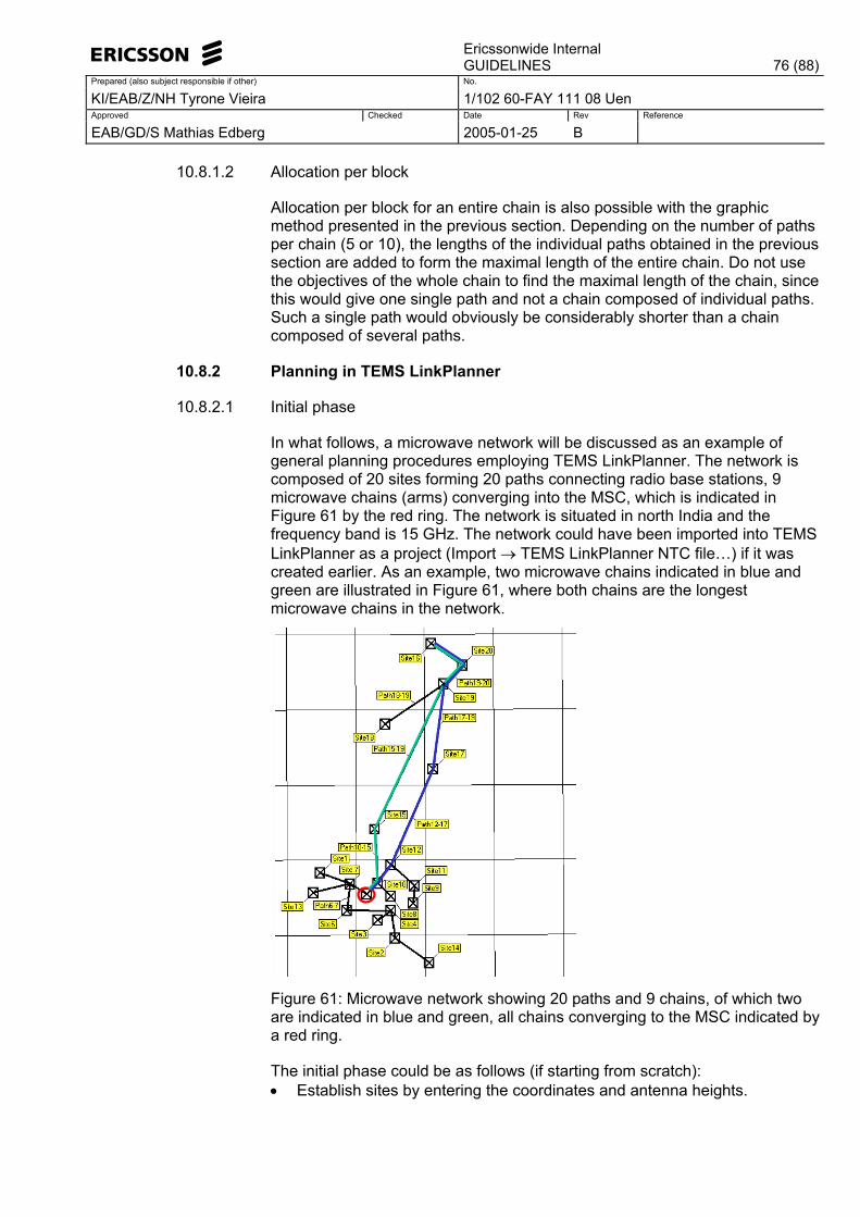
Ericssonwide Internal
GUIDELINES 76 (88)Prepared (also subject responsible if other) No.
KI/EAB/Z/NH Tyrone Vieira 1/102 60-FAY 111 08 Uen Approved Checked Date Rev Reference
EAB/GD/S Mathias Edberg 2005-01-25 B
10.8.1.2 Allocation per block
Allocation per block for an entire chain is also possible with the graphic method presented in the previous section. Depending on the number of paths per chain (5 or 10), the lengths of the individual paths obtained in the previous section are added to form the maximal length of the entire chain. Do not use the objectives of the whole chain to find the maximal length of the chain, since this would give one single path and not a chain composed of individual paths. Such a single path would obviously be considerably shorter than a chain composed of several paths.
10.8.2 Planning in TEMS LinkPlanner
10.8.2.1 Initial phase
In what follows, a microwave network will be discussed as an example of general planning procedures employing TEMS LinkPlanner. The network is composed of 20 sites forming 20 paths connecting radio base stations, 9 microwave chains (arms) converging into the MSC, which is indicated in Figure 61 by the red ring. The network is situated in north India and the frequency band is 15 GHz. The network could have been imported into TEMS LinkPlanner as a project (Import → TEMS LinkPlanner NTC file�) if it was created earlier. As an example, two microwave chains indicated in blue and green are illustrated in Figure 61, where both chains are the longest microwave chains in the network.
Figure 61: Microwave network showing 20 paths and 9 chains, of which two are indicated in blue and green, all chains converging to the MSC indicated by a red ring.
The initial phase could be as follows (if starting from scratch): • Establish sites by entering the coordinates and antenna heights.
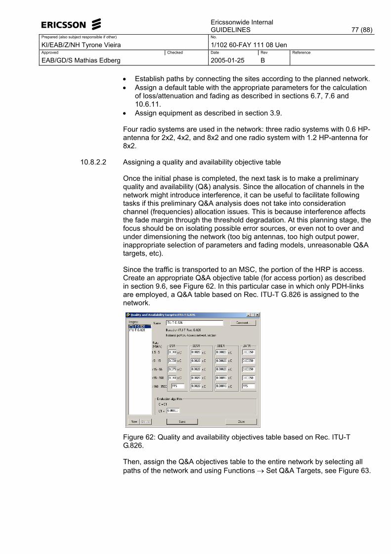
Ericssonwide Internal
GUIDELINES 77 (88)Prepared (also subject responsible if other) No.
KI/EAB/Z/NH Tyrone Vieira 1/102 60-FAY 111 08 Uen Approved Checked Date Rev Reference
EAB/GD/S Mathias Edberg 2005-01-25 B
• Establish paths by connecting the sites according to the planned network. • Assign a default table with the appropriate parameters for the calculation
of loss/attenuation and fading as described in sections 6.7, 7.6 and 10.6.11.
• Assign equipment as described in section 3.9.
Four radio systems are used in the network: three radio systems with 0.6 HP-antenna for 2x2, 4x2, and 8x2 and one radio system with 1.2 HP-antenna for 8x2.
10.8.2.2 Assigning a quality and availability objective table
Once the initial phase is completed, the next task is to make a preliminary quality and availability (Q&) analysis. Since the allocation of channels in the network might introduce interference, it can be useful to facilitate following tasks if this preliminary Q&A analysis does not take into consideration channel (frequencies) allocation issues. This is because interference affects the fade margin through the threshold degradation. At this planning stage, the focus should be on isolating possible error sources, or even not to over and under dimensioning the network (too big antennas, too high output power, inappropriate selection of parameters and fading models, unreasonable Q&A targets, etc).
Since the traffic is transported to an MSC, the portion of the HRP is access. Create an appropriate Q&A objective table (for access portion) as described in section 9.6, see Figure 62. In this particular case in which only PDH-links are employed, a Q&A table based on Rec. ITU-T G.826 is assigned to the network.
Figure 62: Quality and availability objectives table based on Rec. ITU-T G.826.
Then, assign the Q&A objectives table to the entire network by selecting all paths of the network and using Functions → Set Q&A Targets, see Figure 63.
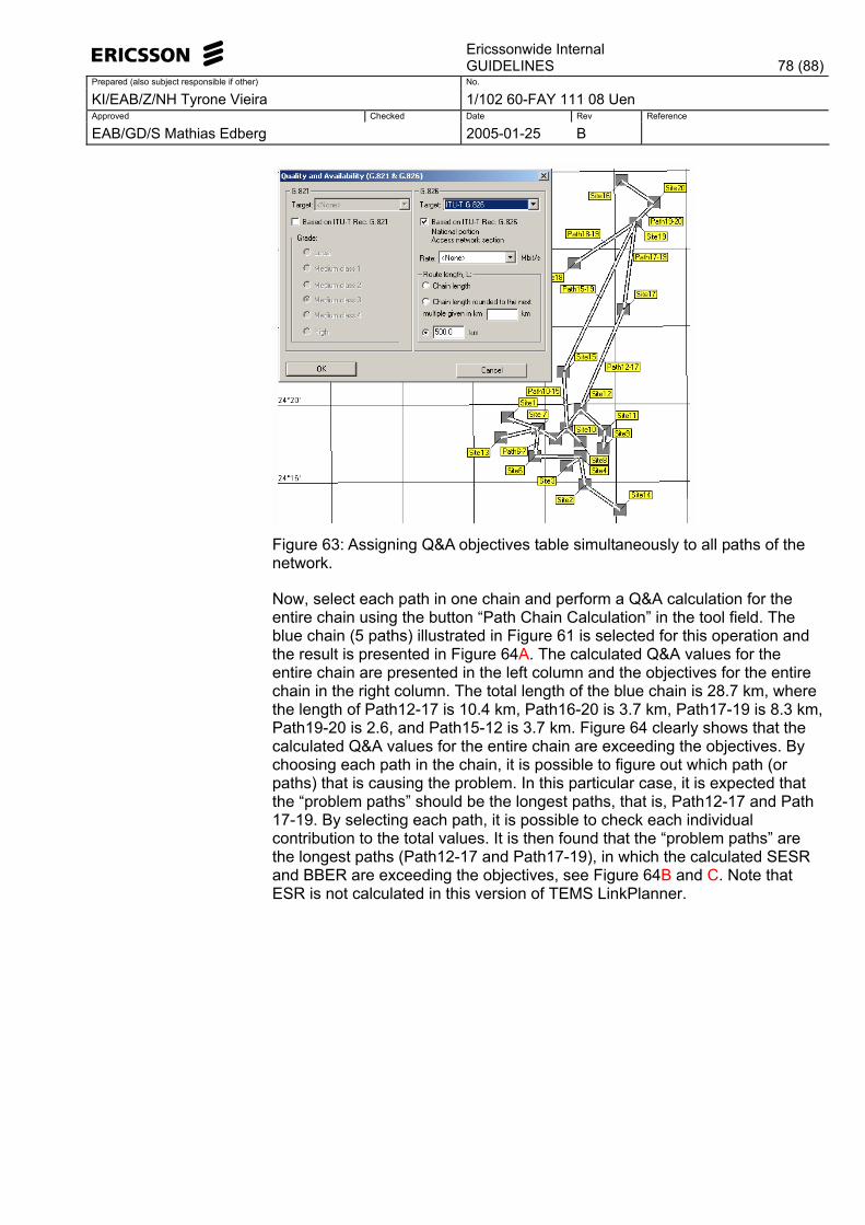
Ericssonwide Internal
GUIDELINES 78 (88)Prepared (also subject responsible if other) No.
KI/EAB/Z/NH Tyrone Vieira 1/102 60-FAY 111 08 Uen Approved Checked Date Rev Reference
EAB/GD/S Mathias Edberg 2005-01-25 B
Figure 63: Assigning Q&A objectives table simultaneously to all paths of the network.
Now, select each path in one chain and perform a Q&A calculation for the entire chain using the button �Path Chain Calculation� in the tool field. The blue chain (5 paths) illustrated in Figure 61 is selected for this operation and the result is presented in Figure 64A. The calculated Q&A values for the entire chain are presented in the left column and the objectives for the entire chain in the right column. The total length of the blue chain is 28.7 km, where the length of Path12-17 is 10.4 km, Path16-20 is 3.7 km, Path17-19 is 8.3 km, Path19-20 is 2.6, and Path15-12 is 3.7 km. Figure 64 clearly shows that the calculated Q&A values for the entire chain are exceeding the objectives. By choosing each path in the chain, it is possible to figure out which path (or paths) that is causing the problem. In this particular case, it is expected that the �problem paths� should be the longest paths, that is, Path12-17 and Path 17-19. By selecting each path, it is possible to check each individual contribution to the total values. It is then found that the �problem paths� are the longest paths (Path12-17 and Path17-19), in which the calculated SESR and BBER are exceeding the objectives, see Figure 64B and C. Note that ESR is not calculated in this version of TEMS LinkPlanner.
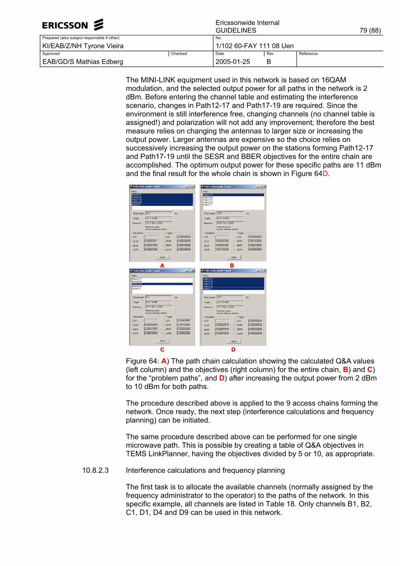
Ericssonwide Internal
GUIDELINES 79 (88)Prepared (also subject responsible if other) No.
KI/EAB/Z/NH Tyrone Vieira 1/102 60-FAY 111 08 Uen Approved Checked Date Rev Reference
EAB/GD/S Mathias Edberg 2005-01-25 B
The MINI-LINK equipment used in this network is based on 16QAM modulation, and the selected output power for all paths in the network is 2 dBm. Before entering the channel table and estimating the interference scenario, changes in Path12-17 and Path17-19 are required. Since the environment is still interference free, changing channels (no channel table is assigned!) and polarization will not add any improvement; therefore the best measure relies on changing the antennas to larger size or increasing the output power. Larger antennas are expensive so the choice relies on successively increasing the output power on the stations forming Path12-17 and Path17-19 until the SESR and BBER objectives for the entire chain are accomplished. The optimum output power for these specific paths are 11 dBm and the final result for the whole chain is shown in Figure 64D.
A
C
B
D
A
C
B
D Figure 64: A) The path chain calculation showing the calculated Q&A values (left column) and the objectives (right column) for the entire chain, B) and C) for the �problem paths�, and D) after increasing the output power from 2 dBm to 10 dBm for both paths.
The procedure described above is applied to the 9 access chains forming the network. Once ready, the next step (interference calculations and frequency planning) can be initiated.
The same procedure described above can be performed for one single microwave path. This is possible by creating a table of Q&A objectives in TEMS LinkPlanner, having the objectives divided by 5 or 10, as appropriate.
10.8.2.3 Interference calculations and frequency planning
The first task is to allocate the available channels (normally assigned by the frequency administrator to the operator) to the paths of the network. In this specific example, all channels are listed in Table 18. Only channels B1, B2, C1, D1, D4 and D9 can be used in this network.
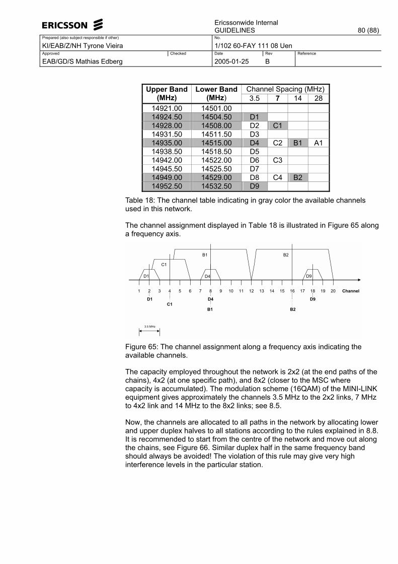
Ericssonwide Internal
GUIDELINES 80 (88)Prepared (also subject responsible if other) No.
KI/EAB/Z/NH Tyrone Vieira 1/102 60-FAY 111 08 Uen Approved Checked Date Rev Reference
EAB/GD/S Mathias Edberg 2005-01-25 B
Channel Spacing (MHz) Upper Band
(MHz) Lower Band
(MHz) 3.5 7 14 28 14921.00 14501.00 14924.50 14504.50 D1 14928.00 14508.00 D2 C1 14931.50 14511.50 D3 14935.00 14515.00 D4 C2 B1 A1 14938.50 14518.50 D5 14942.00 14522.00 D6 C3 14945.50 14525.50 D7 14949.00 14529.00 D8 C4 B2 14952.50 14532.50 D9
Table 18: The channel table indicating in gray color the available channels used in this network.
The channel assignment displayed in Table 18 is illustrated in Figure 65 along a frequency axis.
Channel1 92 3 4 5 6 7 8 10 11 12 13 14 15 16 17 18 19 20
D1C1
D4
B2
D9
B1
D1
C1
D4
B1 B2
D9
3.5 MHz
Figure 65: The channel assignment along a frequency axis indicating the available channels.
The capacity employed throughout the network is 2x2 (at the end paths of the chains), 4x2 (at one specific path), and 8x2 (closer to the MSC where capacity is accumulated). The modulation scheme (16QAM) of the MINI-LINK equipment gives approximately the channels 3.5 MHz to the 2x2 links, 7 MHz to 4x2 link and 14 MHz to the 8x2 links; see 8.5.
Now, the channels are allocated to all paths in the network by allocating lower and upper duplex halves to all stations according to the rules explained in 8.8. It is recommended to start from the centre of the network and move out along the chains, see Figure 66. Similar duplex half in the same frequency band should always be avoided! The violation of this rule may give very high interference levels in the particular station.
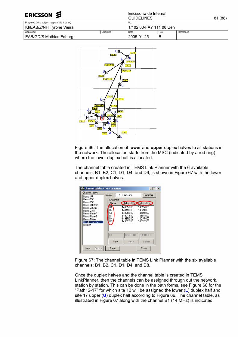
Ericssonwide Internal
GUIDELINES 81 (88)Prepared (also subject responsible if other) No.
KI/EAB/Z/NH Tyrone Vieira 1/102 60-FAY 111 08 Uen Approved Checked Date Rev Reference
EAB/GD/S Mathias Edberg 2005-01-25 B
UU
U
U
U
U
U
L
LL
L
L
L
UU
U
U
LU
L
UU
U
U
U
U
U
L
LL
L
L
L
UU
U
U
LU
L
Figure 66: The allocation of lower and upper duplex halves to all stations in the network. The allocation starts from the MSC (indicated by a red ring) where the lower duplex half is allocated.
The channel table created in TEMS Link Planner with the 6 available channels: B1, B2, C1, D1, D4, and D9, is shown in Figure 67 with the lower and upper duplex halves.
Figure 67: The channel table in TEMS Link Planner with the six available channels: B1, B2, C1, D1, D4, and D8.
Once the duplex halves and the channel table is created in TEMS LinkPlanner, then the channels can be assigned through out the network, station by station. This can be done in the path forms, see Figure 68 for the �Path12-17� for which site 12 will be assigned the lower (L) duplex half and site 17 upper (U) duplex half according to Figure 66. The channel table, as illustrated in Figure 67 along with the channel B1 (14 MHz) is indicated.
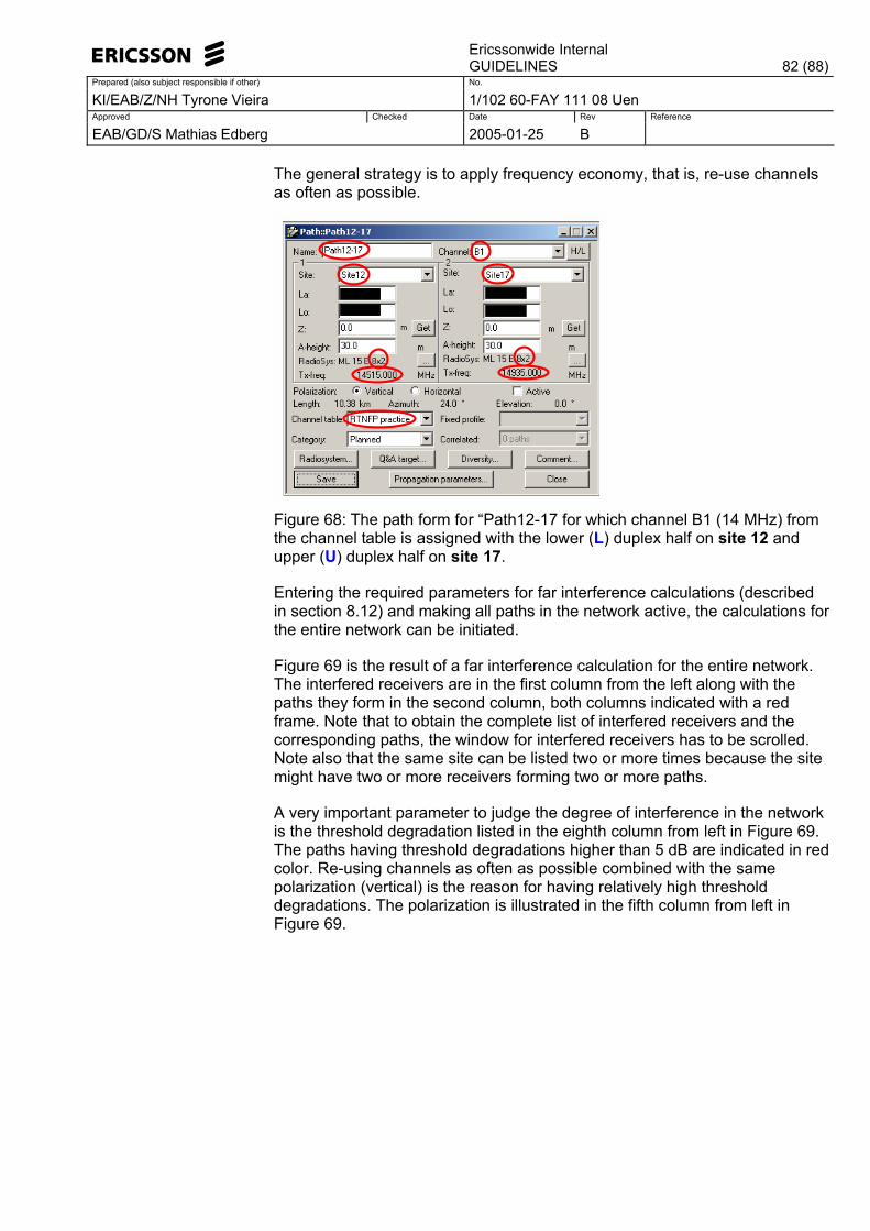
Ericssonwide Internal
GUIDELINES 82 (88)Prepared (also subject responsible if other) No.
KI/EAB/Z/NH Tyrone Vieira 1/102 60-FAY 111 08 Uen Approved Checked Date Rev Reference
EAB/GD/S Mathias Edberg 2005-01-25 B
The general strategy is to apply frequency economy, that is, re-use channels as often as possible.
Figure 68: The path form for �Path12-17 for which channel B1 (14 MHz) from the channel table is assigned with the lower (L) duplex half on site 12 and upper (U) duplex half on site 17.
Entering the required parameters for far interference calculations (described in section 8.12) and making all paths in the network active, the calculations for the entire network can be initiated.
Figure 69 is the result of a far interference calculation for the entire network. The interfered receivers are in the first column from the left along with the paths they form in the second column, both columns indicated with a red frame. Note that to obtain the complete list of interfered receivers and the corresponding paths, the window for interfered receivers has to be scrolled. Note also that the same site can be listed two or more times because the site might have two or more receivers forming two or more paths.
A very important parameter to judge the degree of interference in the network is the threshold degradation listed in the eighth column from left in Figure 69. The paths having threshold degradations higher than 5 dB are indicated in red color. Re-using channels as often as possible combined with the same polarization (vertical) is the reason for having relatively high threshold degradations. The polarization is illustrated in the fifth column from left in Figure 69.
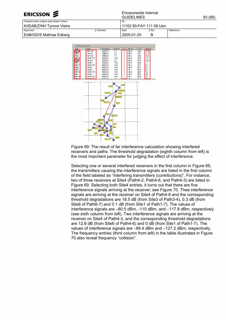
Ericssonwide Internal
GUIDELINES 83 (88)Prepared (also subject responsible if other) No.
KI/EAB/Z/NH Tyrone Vieira 1/102 60-FAY 111 08 Uen Approved Checked Date Rev Reference
EAB/GD/S Mathias Edberg 2005-01-25 B
Figure 69: The result of far interference calculation showing interfered receivers and paths. The threshold degradation (eighth column from left) is the most important parameter for judging the effect of interference.
Selecting one or several interfered receivers in the first column in Figure 69, the transmitters causing the interference signals are listed in the first column of the field labeled as �interfering transmitters (contributions)�. For instance, two of three receivers at Site4 (Path4-2, Path4-6, and Path4-3) are listed in Figure 69. Selecting both Site4 entries, it turns out that there are five interference signals arriving at the receiver; see Figure 70. Thee interference signals are arriving at the receiver on Site4 of Path4-6 and the corresponding threshold degradations are 18.5 dB (from Site3 of Path3-4), 0.3 dB (from Site6 of Path6-7) and 0.1 dB (from Site1 of Path1-7). The values of interference signals are �80.5 dBm, -110 dBm, and �117.8 dBm, respectively (see sixth column from left). Two interference signals are arriving at the receiver on Site4 of Path4-3, and the corresponding threshold degradations are 12.8 dB (from Site6 of Path4-6) and 0 dB (from Site1 of Path1-7). The values of interference signals are �89.4 dBm and �127.2 dBm, respectively. The frequency entries (third column from left) in the table illustrated in Figure 70 also reveal frequency �collision�.
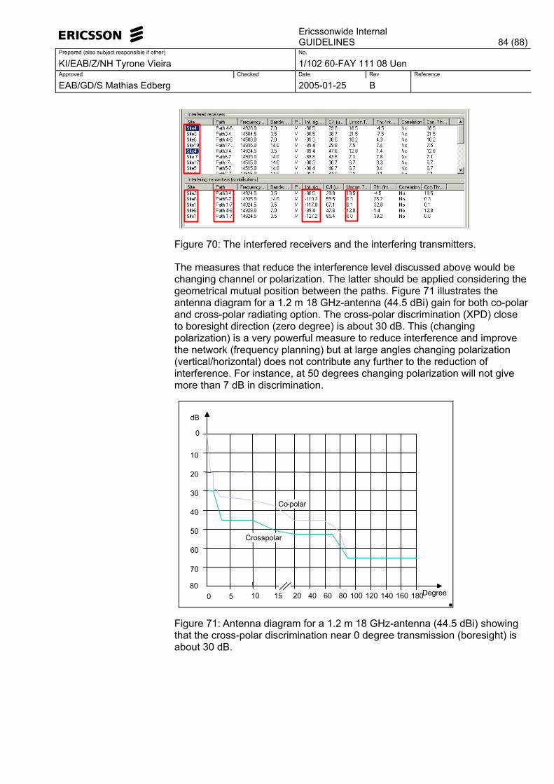
Ericssonwide Internal
GUIDELINES 84 (88)Prepared (also subject responsible if other) No.
KI/EAB/Z/NH Tyrone Vieira 1/102 60-FAY 111 08 Uen Approved Checked Date Rev Reference
EAB/GD/S Mathias Edberg 2005-01-25 B
Figure 70: The interfered receivers and the interfering transmitters.
The measures that reduce the interference level discussed above would be changing channel or polarization. The latter should be applied considering the geometrical mutual position between the paths. Figure 71 illustrates the antenna diagram for a 1.2 m 18 GHz-antenna (44.5 dBi) gain for both co-polar and cross-polar radiating option. The cross-polar discrimination (XPD) close to boresight direction (zero degree) is about 30 dB. This (changing polarization) is a very powerful measure to reduce interference and improve the network (frequency planning) but at large angles changing polarization (vertical/horizontal) does not contribute any further to the reduction of interference. For instance, at 50 degrees changing polarization will not give more than 7 dB in discrimination.
0 5 10 15
0
10
30
20
50
40
70
60
80
dB
Degree 20 40 60 80 100 120 140 160 180
Co-polar
Cross-polar
Figure 71: Antenna diagram for a 1.2 m 18 GHz-antenna (44.5 dBi) showing that the cross-polar discrimination near 0 degree transmission (boresight) is about 30 dB.

Ericssonwide Internal
GUIDELINES 85 (88)Prepared (also subject responsible if other) No.
KI/EAB/Z/NH Tyrone Vieira 1/102 60-FAY 111 08 Uen Approved Checked Date Rev Reference
EAB/GD/S Mathias Edberg 2005-01-25 B
Lets return to the blue chain illustrated on Figure 61. One particular path of this chain (Path17-19) is affected by interference; see Figure 69. In analogy to the previous explanation, there are interference signals arriving at the receiver on Site17 and Site19, see Figure 72. For instance, the threshold degradation on Site19 from Site15 (Path15-19) is 7.4 dB and that might certainly affect the Q&A results.
Figure 72: The interfered receivers on Path17-19 of the blue chain and the interfering transmitters from other paths.
When performing a new Q&A calculation for the blue chain, see Figure 73, it turns out that the interference signals has affected the Q&A parameter (BBER), and the responsible for the BBER deterioration in the blue chain is the interference signals arriving at Path17-19.
Figure 73: The responsible for the deterioration of the Q&A values (BBER) of the blue chain is the interference signals arriving at Path17-19.
Now, the next step is to take a measure in order to reduce the level of the interference signals arriving at Path17-19. Changing channels or polarization is a reasonable approach, provided that the changes do not cause more interference in the network. The output power of all paths is kept at the same level!
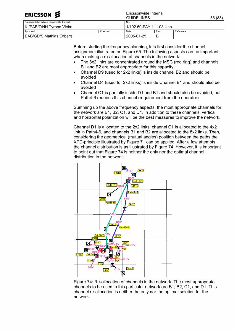
Ericssonwide Internal
GUIDELINES 86 (88)Prepared (also subject responsible if other) No.
KI/EAB/Z/NH Tyrone Vieira 1/102 60-FAY 111 08 Uen Approved Checked Date Rev Reference
EAB/GD/S Mathias Edberg 2005-01-25 B
Before starting the frequency planning, lets first consider the channel assignment illustrated on Figure 65. The following aspects can be important when making a re-allocation of channels in the network: • The 8x2 links are concentrated around the MSC (red ring) and channels
B1 and B2 are most appropriate for this capacity • Channel D9 (used for 2x2 links) is inside channel B2 and should be
avoided • Channel D4 (used for 2x2 links) is inside Channel B1 and should also be
avoided • Channel C1 is partially inside D1 and B1 and should also be avoided, but
Path4-6 requires this channel (requirement from the operator)
Summing up the above frequency aspects, the most appropriate channels for the network are B1, B2, C1, and D1. In addition to these channels, vertical and horizontal polarization will be the best measures to improve the network.
Channel D1 is allocated to the 2x2 links, channel C1 is allocated to the 4x2 link in Path4-6, and channels B1 and B2 are allocated to the 8x2 links. Then, considering the geometrical (mutual angles) position between the paths the XPD-principle illustrated by Figure 71 can be applied. After a few attempts, the channel distribution is as illustrated by Figure 74. However, it is important to point out that Figure 74 is neither the only nor the optimal channel distribution in the network.
B1/V
B1/V
B2/V
B2/V
B2/V
B2/H
B2/H
B2/H
D1/V
D1/V
D1/V
D1/HD1/H
D1/H
C1/H
D1/V D1/V
D1/H
D1/V
D1/H
B1/V
B1/V
B2/V
B2/V
B2/V
B2/H
B2/H
B2/H
D1/V
D1/V
D1/V
D1/HD1/H
D1/H
C1/H
D1/V D1/V
D1/H
D1/V
D1/H
Figure 74: Re-allocation of channels in the network. The most appropriate channels to be used in this particular network are B1, B2, C1, and D1. This channel re-allocation is neither the only nor the optimal solution for the network.
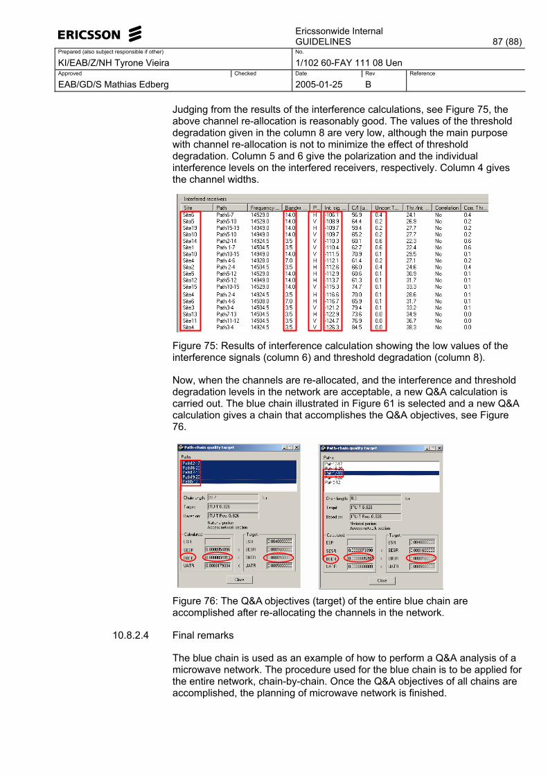
Ericssonwide Internal
GUIDELINES 87 (88)Prepared (also subject responsible if other) No.
KI/EAB/Z/NH Tyrone Vieira 1/102 60-FAY 111 08 Uen Approved Checked Date Rev Reference
EAB/GD/S Mathias Edberg 2005-01-25 B
Judging from the results of the interference calculations, see Figure 75, the above channel re-allocation is reasonably good. The values of the threshold degradation given in the column 8 are very low, although the main purpose with channel re-allocation is not to minimize the effect of threshold degradation. Column 5 and 6 give the polarization and the individual interference levels on the interfered receivers, respectively. Column 4 gives the channel widths.
Figure 75: Results of interference calculation showing the low values of the interference signals (column 6) and threshold degradation (column 8).
Now, when the channels are re-allocated, and the interference and threshold degradation levels in the network are acceptable, a new Q&A calculation is carried out. The blue chain illustrated in Figure 61 is selected and a new Q&A calculation gives a chain that accomplishes the Q&A objectives, see Figure 76.
Figure 76: The Q&A objectives (target) of the entire blue chain are accomplished after re-allocating the channels in the network.
10.8.2.4 Final remarks
The blue chain is used as an example of how to perform a Q&A analysis of a microwave network. The procedure used for the blue chain is to be applied for the entire network, chain-by-chain. Once the Q&A objectives of all chains are accomplished, the planning of microwave network is finished.
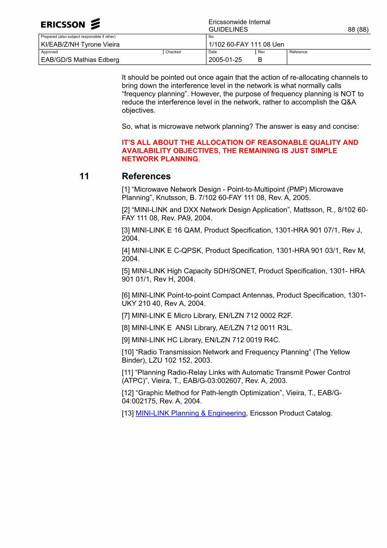
Ericssonwide Internal
GUIDELINES 88 (88)Prepared (also subject responsible if other) No.
KI/EAB/Z/NH Tyrone Vieira 1/102 60-FAY 111 08 Uen Approved Checked Date Rev Reference
EAB/GD/S Mathias Edberg 2005-01-25 B
It should be pointed out once again that the action of re-allocating channels to bring down the interference level in the network is what normally calls �frequency planning�. However, the purpose of frequency planning is NOT to reduce the interference level in the network, rather to accomplish the Q&A objectives.
So, what is microwave network planning? The answer is easy and concise:
IT�S ALL ABOUT THE ALLOCATION OF REASONABLE QUALITY AND AVAILABILITY OBJECTIVES, THE REMAINING IS JUST SIMPLE NETWORK PLANNING.
11 References [1] �Microwave Network Design - Point-to-Multipoint (PMP) Microwave Planning�, Knutsson, B. 7/102 60-FAY 111 08, Rev. A, 2005.
[2] �MINI-LINK and DXX Network Design Application�, Mattsson, R., 8/102 60-FAY 111 08, Rev. PA9, 2004.
[3] MINI-LINK E 16 QAM, Product Specification, 1301-HRA 901 07/1, Rev J, 2004.
[4] MINI-LINK E C-QPSK, Product Specification, 1301-HRA 901 03/1, Rev M, 2004.
[5] MINI-LINK High Capacity SDH/SONET, Product Specification, 1301- HRA 901 01/1, Rev H, 2004.
[6] MINI-LINK Point-to-point Compact Antennas, Product Specification, 1301-UKY 210 40, Rev A, 2004.
[7] MINI-LINK E Micro Library, EN/LZN 712 0002 R2F.
[8] MINI-LINK E ANSI Library, AE/LZN 712 0011 R3L.
[9] MINI-LINK HC Library, EN/LZN 712 0019 R4C.
[10] �Radio Transmission Network and Frequency Planning� (The Yellow Binder), LZU 102 152, 2003.
[11] �Planning Radio-Relay Links with Automatic Transmit Power Control (ATPC)�, Vieira, T., EAB/G-03:002607, Rev. A, 2003.
[12] �Graphic Method for Path-length Optimization�, Vieira, T., EAB/G-04:002175, Rev. A, 2004.
[13] MINI-LINK Planning & Engineering, Ericsson Product Catalog.