Mutual Fund Trading and Liquidity

by

Ka Yin Kevin Chu

B.A., University of Chicago(2001)M.Eng., Columbia University(2002)

Submitted to the MIT Sloan School of Managementin partial fulfillment of the requirements for the degree of

Master of Science

at the

MASSACHUSETTS INSTITUTE OF TECHNOLOGY

February 2010

@ Massachusetts Institute of Technology 2010. All rights reserved.

A uthor ............................ MIT.......MIT Sfoan School of Management

January 15, 2010

Certified by ...................

iang/WagMizuho Financial Group Professor

Thesis Supervisor

A ccepted by ........ ... .......................Ezra W. Zuckerman

Nanyang Technology University Associate Professor of StrategicManagement and Economic Sociology

Chairman, Doctoral Program

MASSACHUSE S INSTrEOF TECHNOLOGY

FEB 0 9 2010

LIBRARIES

ARCHIVES

Mutual Fund Trading and Liquidity

by

Ka Yin Kevin Chu

Submitted to the MIT Sloan School of Managementon 15 January 2010, in partial fulfillment of the

requirements for the degree ofMaster of Science

Abstract

This thesis uses equities holdings snapshots of mutual funds to study their trading pat-terns.Using quarter and semi-annual holdings of mutual funds, I am able to extract amain trading component with the application of the asymptotic principle componentmethod. This component demonstrates short term predictability of returns over threemonths, suggesting overall mutual fund trades contain a liquidity trading componentthat temporarily pushes up stock prices that reverse over the next few months. I alsodemonstrates that this particular type of liquidity risk is related to other meausres of liq-uidity risk. Therefore, this trading component can be a useful building block in creatinga comprehensive measure of liquidity.

Thesis Supervisor: Jiang WangTitle: Mizuho Financial Group Professor

Acknowledgements

This work would not have been completed without help and supportof many individuals. I would like to thank everyone who has helpedme along the way. Particularly: Professor Jiang Wang providing me anopportunity to conduct my research under him and for his guidance and

support over the course of it. Professor Jun Pan for valuable researchadvice, and my fellow schoolmates at Sloan for support and suggestions.

My thanks also goes to my friends and especially my family, for theirsupport throughout my time at Sloan. Without their encouragementand emotional support this would not be possible.

Contents

1 Introduction

1.1 Background and motivations for research . .................

1.2 Related Literature .............................

2 Data and research design

2.1 Data .................................

2.1.1 Data description ......

2.1.2 Stock-level trading activity .

2.1.3 Data filters and scaling ...

2.2 Research Design and theory ........

2.2.1 Theory . ...............

2.3 Asymptotic Principal Factor . .......

2.3.1 Extraction of Common component

2.3.2 Theory . ...............

2.3.3 Application . ............

2.3.4 Properties of principle factor . .

. . . . .. . . . . . . .. . . . . . .. 1 1

. . . . . . . . . . . . . . . . . . . . . 13

. . . .. . . . . . . .. . . . . . .. . 14

. . . . o. . . . . . . . .

..............

3 Results

3.1 Time Series Regression ..........

3.1.1 Description of Time Series Results

3.1.2 Discussing Time Series Results

3.2 Cross-section tests . ............

3.2.1 Identifying innovations in liquidity

3.2.2 Pre-ranking betas ..........

Postranking portfolio betas . .

A lphas . . . . . . . . . . . . . . . .

Estimating Risk Premium using All

Sorting by liquidity measures . . .

Sorting by predicted liquidity betas

Discussion on Cross-Section tests .

10 Portfolios . ........ 29

. . . . . . . . . . . . . . . . . 29

. . . . . . . . . . . . . . . . . 32

. . . . . . . . . . . . . . . . . 33

4 Conclusion

5 Appendix

5.1 A simple version of ICAPM ........................

5.1.1 M odel set-up . . . . . . . . . . . . . . . . . . . . . . . . . . . .

5.1.2 Equilibrium ............ ... .. ...........

5.1.3 P roof . . . . . . . . . . . . . . . . . . . . . . . . . . . . . . . .

5.2 Further time-series analysis based on subperiod and subsample analysis

5.3 Graphs and Tables .............................

3.2.3

3.2.4

3.2.5

3.2.6

3.2.7

3.2.8

36

36

36

37

38

40

41

Chapter 1

Introduction

1.1 Background and motivations for research

There is extensive literature on liquidity. Broadly defined as the ability to trade quickly

and at low cost, episodes such as the breakdown of Long Term Capital Management and

the recent mortgage meltdown highlighted the downside of holding illiquid assets, and

question whether aggregate liquidity should be a risk factor in asset pricing. In light of

the unfavorable nature of holding illiquid assets, it appears that aggregate liquidity risk

should be a priced risk factor in the economy. This is further supported by the recent

credit crisis, where the cost of liquidity drives several investment banks out of existence,

and a market crash that is not seen since the Great Depression.

One branch of the empirical literature aim to identify stocks with different level of

liquidity through characteristics and compare their returns. Examples of these includes

Amihud(2002), Amihud and Mendelson (1986), Brennan and Subrahmanyam (1996),

Brennan, Chordia and Subrahmanyam (1998), Datar, Naik, Radcliffe (1998), etc. An-

other branch sought to identify liquidity-based trading directly and study its effects.

These includes Campbell, Grossman and Wang (1993), Lo and Wang(2000,2006), Pastor

and Stambaugh (2003) etc., usually by stock volume. The difficulty of these papers is

that volume is not signed, and one can only observe total trades of a stock, which is the

sum of liquidity-based trades and information-based trades.

On the other hand, there is research making use mutual fund holdings. In a series

of papers Daniel, Grinblatt, Titman, and Wermers showed that mutual fund trading is

related to momentum, and momentum could possibly explain most of the alphas of funds.

Lamont and Farazzini (2006) finds that stocks that are bought up by mutual funds have

low return in the long run.

This paper aim at bridging the gap between these two literatures, using mutual fund

trading as a better proxy for liquidity trades and study its asset pricing implications.

I consider mutual fund trading as a candidate for this study for a number of reasons.

Mutual funds made up a substantial part of the US stock market. Equities trading

mutual funds are all long in the market and use very little leverage or short selling. Also,

it is known that mutual funds are forced to engage in liquidity trades. If a fund's focus is

technology stocks and the fund experience large inflow, then the manger is forced to buy

stocks in the technology sector even if he believes that the sector is overpriced overall.

The fact that many funds index their performance to benchmark such as the S&P 500

also encourage funds to rebalance their portfolio when the benchmark changes, or in the

case of index funds, essentially forcing them to engage in liquidity trades that creates

short term price fluctuations. (Petajisto 2008)

I find that a liquidity component can be extracted from quarterly change of portfolio

holding of mutual funds. This factor is able to predict market return, share the properties

of many commonly used proxies for liquidity. In addition, in cross sectional test I found

some evidence of the sensitivity of liquidity risk is priced in the cross section.

In this paper I do not investigate the question whether (individual) mutual fund

outperforms the market. Instead I investigate if aggregated mutual fund trades contain

component(s) that are related to market-wide liquidity. The paper is organized as follows:

Chapter 2 discuss the data, a model that relate liquidity trades to stock returns and the

asymptotic principle component method I employ to obtain the liquidity factor. Chapter

3 presents the time-series and cross-section results I obtained.

1.2 Related Literature

My research is related to the papers on the relation between returns and volumes. Some

early paper focuses on relations between daily market returns and volume (For example,

Duffee(1992), Gallant, Rossi and Tauchen(1992) and Campbell, Grossman and Wang

(1993)). These paper finds that returns on high-volume days have a tendency to reverse

in the next few days. Llorente, Michaely, Saar and Wang (2002) finds that returns

accompanied by high volume tends to reverse itself for firms with low level of information

asymmetry and that the opposite takes place for firms with high information asymmetry.

These paper focuses on daily frequency of returns. My paper uses return of longer horizon

and also use the actual trading of the mutual fund industry. This has the benefit of

distinguishing buys from sells, whereas in volume both buys and sells contribute positively

to volume.

This paper is also related to the literature on mutual fund performance and flows.

A large body of the literature is about whether it is possible to pick mutual funds that

consistently outperform it peers. Grinblatt and Titman (1989a,1993) finds that some

mutual fund managers are able to consistently earn positive abnormal returns before

fees and expenses. A collection of paper using a large database of mutual fund holdings

[Grinblatt, Titman and Wermers (1995), Wermers (1997), Chen, Jegadeesh and Werm-

ers(2000)] finds that majority of mutual funds to pursue an active momentum strategy

and that the best-performaning funds use their inflow to buy winner stocks that produces

superior returns'. Consistent with this, Cahart(1997) finds that after controlling for mo-

mentum, there is no predictable abnormal returns in the best funds. To the opposite

'Other research has reached a smimalr concolusion using a different data set which contains thetrading of all institutions. For reference, see Burch and Swaminathan (2001), Badrinath and Wahal(2002) and Sias (2004, 2007)

end, the paper of Cahart, and the papers by Brown and Goetzmann(1995), Berk and

Tonks (2007) also documents that the worst performing fund seems to consistently un-

derperform in the future. However, that may be a topic of lesser interest because there is

no way to short these bad mutual funds. Recently there are papers that argues that it is

possible to pick fund managers more sophisticated methods. Theses includes: Mamaysky,

Spiegel and Zhang (2004), which correct for systematic bias in estimating risk-adjusted

fund performance; Aramov and Wermers (2004), which uses a trading strategy that in-

corporate predictable manager skills related to industry effect; Kacperczyk, Sialm and

Zheng (2005) found that funds with higher industry concentration holdings have higher

returns both in a 4-factor model and with the DGTW performance measure (in stock

selectability); and Cohen, Coval and Pastor (2005), where they distinguish funds that

outperform due to commonality of the stocks held from manager who outperform due to

stocks traded in the manager's portfolio.

Another class of the literature is focused on the relation between fund returns and

fund flows, as defined as new money invested in a mutual fund (inflow) minus the net

withdrawal from a fund (outflow). Coval and Stafford (2007) found that stocks being

sold by distressed funds underperform in the short term (with reversal), confirming an

asset fire-sale story. My paper also address to this area of research. On one hand, while

manager picks stocks within their fund objective, a large part of their trades are flow

driven (for example, if a technology stock fund manager receive a large investment, he

has to invest mainly in technology stocks no matter what he thinks of the relative value

of technology stocks to stocks in other sectors). Therefore, even if managers are able to

pick stocks, that does not mean all their trades are information based. My paper studies

the effect of the overall trading and try to access whether the majority of trades are based

on superior information.

This paper is also related to the literature on liquidity. Liquidity is a vague con-

cept related to cost related to execution of trading, and much of the literature focuses

on discovering measures of liquidity and whether liquidity risk is priced. For example,

Chordia, Sarkar and Subrahmanyam (2005) explores cross-market liquidity dynamics by

estimating a vector autoregressive model for liquidity (bid-ask spread and depth, returns,

volatility, and order flow in the stock and Treasury bond markets). Pastor and Stam-

baugh (2006) used price reversal caused by volume to measure stock liquidity, and Lo

and Wang (2006) studies daily returns to identify hedging portfolios and test if they can

predict future returns, and if they are priced in the cross-section. My paper contribute

to the literature by arguing that useful information about aggregate market liquidity can

be gathered from trades of mutual funds, supplying additional information to identify all

sources of liquidity risk.

Chapter 2

Data and research design

2.1 Data

2.1.1 Data description

I obtain mutual fund holdings from the Thompson financial CDA/Spectrum Mutual Fund

Holding database. This database covers almost all historical domestic mutual funds plus

about 3,000 global funds that hold a fraction of assets in stocks traded in U.S. exchanges

as well as Canadian stock market. It collects holdings data for each fund from their SEC

N-30D filings, starting from 1980. Thompson financial also use fund prospectus and if

necessary, contact funds for updates or additional data.

The SEC filings include the name of the stock, the number of shares held and the

market value as of the reporting date. Short positions are not reported. Thompson finan-

cial merge this with their stock database to include fund information such as investment

objective, total net assets, management company name and location. They also include

stock information such as CUSIP, ticker, exchange code, share class, quarter end price

and share outstanding. However, it has been found the stock information from Thomp-

son Financial contain errors (Boldin and Ding 2008), therefore I only use their CUSIP

field to match the data with the Center for Research in Security Prices (CRSP) monthly

stock file, and use stock characteristics supplied by CRSP instead for more accurate

information.

The companies are only required to file their holdings semi-annually', but many funds

report their holdings in the other two fiscal quarters as well. These are collected in the

database as well, therefore quarterly portfolio snapshots for a large proportion of funds

are available.

For my analysis I imposed a few data screens:

- I only use observations at the end of calendar quarters (March, June, September

and December).

- I only keep domestic funds with investment objective that is Aggressive Growth,

Growth, Growth and Income, or Balanced.

- Only common stocks traded in NYSE, AMEX or NASDAQ, that can be matched

to the CRSP equity data base (stock code 10 or 11). There are 15,304 such stocks in my

sample.

- Data is available from June 1980 up to March 2007 for a total of 108 quarterly

observations.

Overall these funds covers 46% of common stocks covered by CRSP and covers about

3% of the market cap of these stocks in 1980, and the numbers steadily grows to 90%

coverage and 13% market value in 2006. See Graph 1.1 for a description of the stock

coverage and market share (as a percentage to the market) of mutual funds in my sample.

Stock return, price, share outstanding are from the CRSP, book-to-market ratios

from COMPUSTAT annual files, and the stock market excess returns, small-minus-big,

high-minus-low and winner-minus-loser returns are from Ken French's website.

'Quarterly reports are required before 1985

2.1.2 Stock-level trading activity

After collecting all valid observations, I have a collection of all quarter-to-quarter change

in stock position on each stock, by each mutual fund. But the data is very sparse as very

few funds survive the whole sample period. They also do not hold all the stocks every

quarter. To alleviate this problem, I aggregate the trading of all funds by stock in order

to make the data more densely populated.

For each stock and each quarter, I aggregate the trading of all funds in the stock.

Each quarter I define stock i's net-trading activity (Mit) as

Mit= Ej(ni,,t - ni,)(2.1)Mit = (2.1)Oit

Where nij,t is the number of shares (split-adjusted) held in stock i by fund j , for all

funds that reports holding data for quarter t , and Oit is the split-adjusted number of

share outstanding for stock i. nij,, is the holding of either 1 or 2 quarters ago, using the

more recent holding report available for each fund. Since the database may not report

zero holding in a stock, I set all missing stock holdings to zero. Therefore, if there is a

gap of 6 months between reporting, I assume the change in portfolio in the first quarter

is 0 and the second quarter is the overall change. Portfolio changes with a gap more than

6 months is not used in this analysis.

To avoid errors caused by a surviving fund entering or exiting the sample, if time t

represent the time that a fund appears in the dataset for the first time or if r is the last

time a fund reports its holdings, then these funds are excluded in the calculation of Mit

as their comparing their reported holdings with zero has a high likelihood of creating

outliers in my sample, and do not reflect the actual trading of the fund.

2.1.3 Data filters and scaling

To remove errors, outliers and to drop stocks that are not frequently traded by mutual

funds, I apply these additional data screens:

* I delete all observations where fund j's holding in stock i is larger than its shares

outstanding. This removes any obvious error.

* Stocks that are owned by very few funds are dropped. Define OWNi,t as the number

of funds that has a non-zero holding in stock i, and PCTio,t as the 10-percentile

number of OWNi,t at time t. Then, I only keep mit if it satisfies.

OWNi,t >= min(max(3, PCTio,t), 5) (2.2)

And drops stocks that are owned by very few funds. I utilize a cap and a floor because

the number of funds is small in the early 1980s. I want to remove any stock with very

little coverage and keep stock with sufficient coverage, while keeping the sample more

balanced by adjusting the cutoff as the average stock coverage is higher.

* After filtering out stocks with low ownership, I winsorize the data by dropping the

cross-sectional top and bottom 0.25% stocks (sorted by Mit) for each quarter to

eliminates any remaining outlier.

Interestingly the equal- and value-weighted average Mit have relatively low correlation

(49.9%) with each other, reflecting the difference in trading between large and small

stocks. Since the total size of the mutual fund industry is growing during my sample

period, there are more quarters that funds are buying overall than selling. The time series

averages of the value- and equal-weighted average Mit are 0.1% and 0.2% respectively,

reflecting a steady increase in mutual funds' overall market share. The largest downward

spikes are the last quarter of 1999 and 2002, and are both stronger when I consider the

value-weighted average.

Additionally, the cross-section variance of Mit increase over time, reflecting the in-

creasing trading of the mutual fund industry. Since my measure of trading is closely

related to a fund's trading volume, I scale Mit by dividing the it by the value-weighted

average turnover of all NYSE stocks from the previous twelve months to normalize vari-

ance. Define the variance-scaled Mit as mit:

Mitmit = Mi (2.3)TONYSEt- 12,t

I will be working with mit for the remainder of the article. Graphs 1.2 and 1.3 plots

the value- and equal-weighted average mit. The correlation between mit and Mit is very

high (95.7% for value-weight average and 92.4% for equal-weight averages), showing that

the scaled variable mit still retains much of the information in Mit.

2.2 Research Design and theory

2.2.1 Theory

The analysis is motivation by Merton's ICAPM. The key insights of the ICAPM are

1) Asset returns changes over time if the investment opportunity set is not constant,

and returns follow a factor structure.

For example, in a discrete time model with one state-variable Xt, it can be shown

that excess returns follow the relation:

E(ri) - rf = 3i(rm - rf) + ,3 (rx - rf)

The intuition is that asset returns should only be determined by its covariance with

aggregate wealth and shocks to state variables.

2) Investor's stock portfolio follows two-fund separation.

They invest in the market portfolio and a hedging portfolio, therefore, investor i's

stock holding at time t is equal to:

S = h'itSM + hitSH

where h'Me and h't contains information about investor i's (possibility stochastic)

preference for market risk and hedging demand.

If the investment set opportunity set is constant, then the model reduce to CAPM

where everyone invest only in the risk-free asset and the market portfolio. In addition,

if the change in haut is small compared to hHt, then I can identify SH by considering the

change of positions of the investor over time.

3) The hedging portfolio SH must be the portfolio with the highest predictability of

Xt.

Merton(1973) proved that if one of the asset replicates Xt (interest rate), then the

hedging portfolio consist of that asset (long term bond) only, and clearly these two assets

have a correlation of 1. If the state variable cannot be replicated by an asset, then

the hedging portfolio is the traded portfolio with the highest predictability of Xt (For

example, see Wang and Lo (2006). See Appendix for proof).

This is also intuitive because the hedging portfolio is picked to minimize fluctuation

in investor's utility. The hedging portfolio helps the investor smooth out shocks in the

economy that is attributed to state variables. Suppose investor, instead of investing in the

hedging portfolio, invest in another portfolio with the same betas to the market and to

the state variable. This means that the new portfolio is essentially the hedging portfolio

plus noise (that is not correlated to the market and Xt). Then from (1), this asset will

not earn excess returns. Additionally, this investor will have higher fluctuations in his

wealth, attributed to the deviation from the hedging portfolio. This is a contradiction

and thus the hedging portfolio must have the highest predictability to Xt.

These three predictions support my methodology, which is to identify a main trading

component explain the trading activities of a large set of investors. Using this component

I can analyze its time-series and cross-section predictability and implications.

2.3 Asymptotic Principal Factor

2.3.1 Extraction of Common component

After obtaining stock-level trading activities mit, I need to find a method to extract the

most important information contained in the data. The most commonly used method is

a principle-component analysis, but for my sample I have a cross-section that is much

bigger than the time series. In this case the covariance matrix is singular and I cannot

apply the principle component analysis directly.

A common method used is to group the cross-section into smaller groups (than the

time series) to reduce the size of the cross-section, then apply principle component analy-

sis to the sample with reduced cross-section. However information is lost in the process

and there is not clear-cut way to determine how the data should be summarized.

In this paper I apply an alternate methodology developed by Connor and Korajczyk

(1986, 1988). It is called the Asymptotic Principle Factor and is used for data that

has a large cross-section. This method enables me to extract the principle components

without reducing the size of the cross section. The next section describe the theory and

application of this method.

2.3.2 Theory

In Connor and Korajczyk (1986), they derived a form of APT resulting in a k-factor

model:

i = rf + [ i -+ -j ij3f + i

where ri is the (realized) return for stock i, rf is the risk-free rate and pi the risk

premium for stock i and fj are the realizations of the k factors. Since I do not observe

the k factors directly, I need to estimate them from the data. The problem with financial

data is that the size cross section much bigger than the number of time periods, and

therefore the covariance matrix is singular and I cannot use a direct principle factor

extraction. Connor and Korajczyk suggest using the "asymptotic principle component"

method:

Define B" as the set of /ij's, 7 = {y}j 1 be the vector of factor risk premiums such

that p = B"y, and F to be the set of y + f, the realizations of the factor.

Suppose I observe returns for n stocks over T time periods where n > T. I can write

the observed stock returns in matrix form:

R" = - r = Bn( + f) + E = BF + En

Define theses matrix products:

R" = (1/n)Rn'R

A" = (1/n)F'Bn'BF

Y" = (1/n)(F'Bn'e + E"'BnF)

Zn = (1/n) (,n',n)

And also assume: (existence of average cross-sectional idiosyncratic variance)

U2 = p lim (1/n) nl'n (2.4)n--oo

Notice that QR is the matrix of cross-product of asset excess returns, and Q =

A" + Y" + Z while A n contains information about the true factors. My goal here is to

show that if I extract the principle components from Qn, it will be approximately a linear

transformation of the true factors F. Let H" and An be the eigenvector matrix and the

eigenvalues of A". That is, H"'A" = AnH". Then it can be proved that H" = L"F where

L" is a nonsingular matrix. This is the same as saying that an eigenvalue decomposition

only unique up to a linear transformation. Similarly define Let G" and An be the

eigenvector matrix and the eigenvalues of n", then I would want to show that G" -+ H"

when n is large./The actual proof is technical but a sketch of the proof is provided in

Connor and Korajczyk (1986).

Recall Q" = A" + Y" + Z n . Since E is idiosyncratic noise, it is clear that Y" converges

to zero as they are uncorrelated with the factors. Based on equation 2.4, they also

show that Z n converge to a scalar matrix where all off-diagonal terms are zero. The

eigenvectors of a matrix are unaffected by the addition of a scalar matrix., therefore for

large n Gn will be approximately equal to H n , and therefore G" is a approximately a

linear transformation of F.

Connor and Korajczyk (1988) also shows that this technique can be extended to

returns with time-varying average.

2.3.3 Application

After showing the validity of the asymptotic principle component method, I discuss how

I adopt this method below:

Denote by mt the k x T matrix of scaled net-trading activity for all stocks. Assume

mt follows an approximate factor model with time-varying average:

mt = B(ty, + ft) + ct (2.5)

In essence, this is the same as ordinary factor analysis except that the role of the

time-series and cross-section are reversed. Given the matrix of trading of all stocks over

time M = [mit], I first compute the cross-product matrix Q , where

tl 2 mj,tl * mj,t2*m1,2 (2.6)

-- j 1 jtl * 1 j,t2

Over all (mj,tl, mj,t2) pairs. If an observation in the pair is missing (for example, for

a stock that did not survive the whole sample period), then the product is set to zero.

Ij,t is the indicator function which is set to 0 if mj,t is missing and 1 otherwise.

Therefore each item in the above matrix is the simple average of all (mj,tl * mj,t2) where

both items are not missing.

Then the asymptotic principle factors of the is simply obtained by the eigenvectors of

Q. I use this method to extract the principle factor, and the properties of these factors

will be discussed below.

At this point it is worth discussing the effect of missing observations and outliers.

Suppose that stock i only have k valid observations (tl, t2, ...tk). Then stock i will enter

to the sum for 71,-2 only if both T-and T2 and in the set (t 1 , t 2, ... tk). Therefore there

can only be k2 terms involving stock i. This means that the covariance matrix naturally

gives more weight to stocks with more observation, therefore stocks that only appear in

the panel for very few periods is unlikely to affect the covariance matrix.

On the other hand, the same cannot be said for outliers. If mj,,, is an outlier, then it

will affect all the terms ,,, and Q,,, , which will be 2t - 1 terms out of t2 terms in the

covariance matrix, especially ,1,, which includes (mj,,)2.

Therefore, I need to be very careful about eliminating outliers, and this justifies the

winsorization of the data, and the removal of stocks that are only traded by very few

funds, where they are small stocks and often contain big changes in mit.

Then under technical conditions I can identify the realized factor t + ft, which is

equal to the eigenvectors of the matrix m' * mt. Connor and Korajczyk proved that the

eigenvectors converge to the true factors as the number of assets grow to infinity.

2.3.4 Properties of principle factor

I employed the asymptotic principal factor technique to mt. To test the power of my

extracted factor, I regress the value-weighted mt and equal weighted mt against the first

5 factors. The results are summarized in Table 1.4.

In both regressions, the first factor is significantly stronger than all other factors,

in both magnitude and signficance. The first factor also explains a large part of the

variance explained by the first 5 factors. For the value-weighted average, the first factor

explains 29.00% (59.06%) of the variance for the value(equal)-weighted case and while

5 factors explains 33.01% (71.71%), showing that the first factor explains much more of

the commonality in trades than any other factor. Moreover the significance of the other

factors are unstable and can change if I slightly alter out screening procedure, while the

first factor does not change by much.

Therefore, I only use the first factor for the remainder of the paper. Figure 2 plots

the first factor and Table 3a and 3b shows the correlation matrix of the factor with the

Fama-French factors and average net-trading. It appears that the factor is persistent at

least over two quarters and do not decay very quickly. The factor is also not strongly

related to the any Fama-French factors, even if I consider possible lead-lag relations. The

largest correlation is the HML factor and lagged factor, with a correlation of 0.332.

This factor I extracted does not appear to be driven by any of the commonly used

risk-factor, so I move on to explore its time-series and cross-section explanatory power

of stock returns. From here I will name the extracted factor as Zt. Graph 1.5 plots the

factor with the standard deviation scaled to 1.

Chapter 3

Results

In this section, I want to explore the time-series predictability of the liquidity measure.

The factor Zt captures commonality in trading of mutual funds. It is extracted form

the net change in stock holdings by mutual funds, so my results is very relevant to the

field of research between trading and stock returns.

There is ample research on the relationship between stock returns and trading. In

a classical framework relating trades to prices (for example, Kyle(1985)), trades are

information-based and stock returns correlates positively with informational traders as

information is revealed over time through trades. In reality, trades can be motivated

also by rebalancing or shocks to one's non-tradeable portfolio (for example, income).

Wang (1993,1994) demonstrated that in an environment with information asymmetry,

while trades and contemporaneous stock returns will be positively correlated, future stock

returns could either be positively or negatively correlated with current trades depending

on the true motive behind the trade. In analyzing the properties of Zt I can explore what

is the most important factor affecting mutual fund trading decisions.

My results also add to existing research on the relationship between stock returns and

trading volume. One limitation of current research on return/volume relationship is that

trading volume is not signed. Therefore, one cannot identify if volume is contributed

from an active buy or sell. This paper takes a more direct approach and takes the actual

(signed) trading activity and investigate the relationship with current and future stocks

return. Therefore my results will not only able to determine if mutual fund trading

relates to a source of risk, the results will also show if mutual fund is a provider or risk

insurance or demand risk protection.

3.1 Time Series Regression

3.1.1 Description of Time Series Results

I explore the time-series property of Zt by employing the regression model:

Rt = a + bz * Zt-1 + bR * Rt-1 + Xt-1 + Et (3.1)

Where Rt is the return of the (value- or equal-weighted) market portfolio, Zt-1 is my

liquidity factor, and Xt_ 1 is a set of control variables. They include dividend yield, default

spread, term spread, return volatility (VIX, or RVOL: daily return standard deviation of

the value-weighted index over the past 3 months) and the risk-free rate. Table 1.8 and 1.9

shows the result for whole sample (for value and equal weighted returns, respectively),

and Table 1.10 is the subsample 1986-2006, where the VIX index is available.

As shown in Table 1.8, my factor has strong predictability for value-weighted returns.

A one standard deviation change in my factor predicts the market return to be -0.17

standard deviation lower in the subsequent quarter, and is significant at 5%. With

controls, the parameter is between -0.16 and -. 22, and is significant at 10% except for

the last case. In general, adding controls do not change my results, except when the

3-month interest rate and dividend yields are both included. However, in my sample

these two has high correlation (77%), and this may have introduced extra noise in the

errors. Moreover, my point estimate of the regression coefficient for Zt-1 is still very

comparable to the estimate in other regressions. Overall the evidence supports that Zt

can predict future market returns.

Results are weaker for equal weighted returns. Change of one standard deviation

above average in Zt-1 predicts that the return will be lower by 0.11 standard deviation.

The regression coefficient is not significant but still has the same sign. Adding controls

largely leave my result unchanged, except one case where I regress Rt with Zt-1 and

and the term spread I have a coefficient of -0.17 which is significant at 5%. In all other

situations the coefficient changes between -0.06 and -. 013 and are not significant at 10%..

I also present the results of one particular subperiod here. I use the period from 1986-

2006, which is the period where the VIX index is available and I use VIX as a substitute

of RVOL. VIX has the desirable feature of being a forward looking measure of volatility

where RVOL represents volatility in the previous year. Because of a shorter sample, there

may be a decrease in the power of the test. That is confirmed in Table 1.10, where the

results are similar with weaker significance.. Using only Zt- 1, the regression coefficient

is -0.15 and is significant at 10%. VIX (and RVOL) weakens my result to -0.11(-0.16)

and is not significant at 10%, and so is the case where I use both the dividend yield and

the 3-month risk free rate (-0.07, not significant). The other controls do nothing, the

estimates ranges between -0.16 and -0.18 and are significant at 10%

As an additional test, I also divide the time series into two subperiod of equal length

and repeat my regressions. In each subperiod the regression coefficients remain stable,

and the results are presented in the Appendix.

3.1.2 Discussing Time Series Results

The most important result from this section is that a high level of Zt indicates that the

market return will be lower in the future. In the context of liquidity, this is consistent

with mutual fund demands liquidity, as demand in stocks drive up prices temporarily

and drive down future returns. This result is also consistent with results by Wermers

(2000) where purchase of mutual funds caused by capital inflow drives up stock prices

temporarily, and also the results by Lamont and Farazzini (2006) where stock purchases

made by mutual fund has low returns in the long run. This also suggests that the majority

of trades made by mutual funds are for liquidity purpose rather than information, which

is not very surprising given the difficulty in consistently identify funds that trades with

information and outperform the market.

In addition, Zt has stronger predictability on value-weighted returns than equal-

weighted returns in both magnitude and significance. This is likely because large stocks

have higher correlation with each other, but it is also possible that Zt contain more in-

formation about large stocks as they tend to stay in the sample for a longer time period.

This demonstrates the desirability of using the asymptotic principle factor technique as

it picks out the optimal weight for trading in each stock to contribute to the factor with

the most information.

Since the time-series results suggest that mutual fund demands liquidity, I will move

on to a cross-section test to confirm the results of this section. I will use the methods of

Fama-Macbeth to test if the risk correlated to Zt is priced in the cross-section.

3.2 Cross-section tests

In this section I perform cross-section regressions to determine whether a stock's expected

return is related to its sensitivity to my innovations in the trade factor Zt.

3.2.1 Identifying innovations in liquidity

The first step for cross section test is to remove the predictable component of Zt: To

achieve this, I run the AR(1) regression

Zt = a + pZt- 1 + (t (3.2)

Using current and lagged values of Zt. The residuals, (t, are the unexpected change

in liquidity and is used to determine if liquidity risk is priced. It is possible to add other

factors to equation 3.2 (for example, the lagged market return or Fama-French factors)

but the results would not be materially affected. The goal of the cross-section test is to

determine if risk premium in each stock is related to its sensitivity to (t, controlling for

other source of risk premium. The sensitivity of stock i to (t is simply the slop coefficient

on (t in a multiple regression with stock i's return where other asset pricing factors are

included. To investigate whether the stock's expected return is related to /3L, I follow

the methods of Fama and French (1993). At the end of each year, I sort stock based

on their predicted values of 3L and form 10 portfolios where their betas are sufficiently

dispersed. The postranking returns on these portfolios during the next 12 months are

linked across years to form a single return series for each decile portfolio. The excess

returns on those portfolios are then regressed on return-based factors that are commonly

used in empirical asset pricing studies. The extent that the regression intercepts (alphas)

are different from zero explains the component of returns that is explained by /L but not

by exposures to other risk factors.

3.2.2 Pre-ranking betas

For the purpose of portfolio formation, define O1L as the coefficient on (t in a multiple

regression that also includes the three factors of Fama and French(1993).

rt = ai + t + MKT + /3SMB + HMLt + /UMDt + ei, (3.3)

where r, denotes asset i's excess return, MKT denotes the excess return on a broad

market index, and the other two factors, SMB and HML, are payoffs of long-short spreads

constructed by sorting stocks according to their market capitalization and book-to-market

ratio'. This definition captures stock excess return's co-movement with (t that is distinct

from its co-movement from other commonly used factors.

1These factors are directly downloaded from Ken French's website

For each quarter t, I estaimte f for all common stocks traded in AMEX, NASDAQ

or NYSE, using on data available up to and including t, if they satisfy the following

commonly applied data screens:

* Price and return data is available for stock i at time t from the CRSP database,

and stock price at time t is higher than $5 and lower than $1000.

* Quarterly stock return is available for the stock over the past 5 years.

These estimates will be very noisy, as I use a short time horizon to estimates the

betas, and the estimates can be affected by shocks to individual stock returns. My hope

is that despite that the estimate will still allow us to sort stocks by their true betas (to

some extent), and I will re-estimates the loadings once portfolios are formed to obtain

more accurate estimates for my other tests.

3.2.3 Postranking portfolio betas

At the end of each year, stocks are sorted by their pre-ranking liquidity betas and as-

signed to 10 portfolios. The value-weighted average of each portfolio is calculated. The

postranking returns for each portfolio are linked across each year, forming a single return

series for each decile covering the period from January 1984 to December 2006. Then

the post-ranking beta of each decile portfolio is re-estimated using equation 3.2 over

the whole sample period. Panel A of table 1.11 reports the postranking liquidity betas.

Comparing portfolios 1 and 10, I created a spread in liquidity betas, but the difference

is not statistically significant and the betas do not line up in an increasing fashion from

portfolio 1 to 10. Particularly the loadings on portfolios 5 and 6 are low, and the loading

of portfolio 10 is lower than that of portfolios 8 and 9. The largest estimate is 4.06 with a

t-statistic of 1.59, and the smallest value is -3.33 with a t-statistic of -1.95. The difference

between the betas of the top and bottom decile is 5.21, with a t-statistic of 0.9. Overall,

there is positive correlation between the ranking of pre-ranking betas to post-ranking

betas, but there is certainly concern that the pre-ranking betas estimates are not very

precise and do not sort stocks precisely on their true liquidity betas.

Panel B reports the postranking betas of each decile portfolio for Fama-French factor

and the momentum factor. The market risk shows a U-shape pattern, with the extreme

portfolios having higher market risk. Portfolios 1 and 10 has betas of 1.10 and 1.13

respectively, and portfolios 5 and 6 has betas of 0.95 and 0.97. There is a similar pattern

for the SMB and HML factor: Portfolios 1 and 10 has smaller stocks (loadings of 0.09

and 0.63) and low book-to-market ratios (-0.55 and -0.07) while portfolio 5 and 6 have

larger stocks (loadings of -0.10 and -0.31) and value stocks (HML loadings of 0.17 and

0.01). There is very little spread and no pattern for the UMD betas.

3.2.4 Alphas

Panel C reports the alphas of regression of the decile portfolios using the Fama-French

factors (MKT, SMB, HML) only, and in the second line shows the alphas when I regress

with the Fama-French factors plus the momentum factor. If the alphas shows an up-

ward(downward) trend over the portfolios, that will be an indication that there is a

premium(discount) to the risk loading to my liquidity factor. Same as the case of the

postranking betas, the alphas do not line up perfectly with the deciles. However, they

are still positively correlated.

The three- and four-factors alpha are quite similar, except for portfolio 2. The two

alphas have a correlation of 89%. And they both exhibit an upward trend, but the alpha

for portfolio 0 is quite high in both cases. The correlation of the alphas with the liquidity

betas I estimated in the previous part is low (4% for three factor alpha, -7% for four

factor alpha), and this suggests that my asset pricing test in the next part may not yield

significant results, despite the results this and the previous part are pointing to a positive

direction.

3.2.5 Estimating Risk Premium using All 10 Portfolios

In this part I use the methodology of Fama and Macbeth to estimate the risk premium

associated with the risk to (t. Using the beta estimates from the ten postrank portfolios,

I estimate the regression

(L M M S H U (3.4)rit = ai +/3i r i rT +: ++3 r +/ir +ei t

to obtain estimates of (, pM, pS pH and iu for each quarter. My estimates of the risk

premium for each factor is then the time-series average of these slope coefficients, and

the standard error is the time-series standard deviation divided by the square-root of the

number of observations.

My results show that the estimate of the risk premium is insignificant. When I include

liquidity, Fama-French and momentum factors, I find that economically the difference of

returns between the top and bottom decile portfolio due to liquidity is 0.33% per quarter,

or 1.31% per year. But the t-statistic is only 1.15 and not significant. This may imply

that there is no risk premium associated with liquidity, but this could also simply be

caused by the imprecise ranking of stocks when I sort by historical liquidity betas. The

result is also too weak to say much about the sign of the risk premium. Therefore in

the next section I use a different sorting methodology as an attempt to achieve better

sorting.

3.2.6 Sorting by liquidity measures

Sorting by historical liquidity betas yield weak results. This may be due to the fact that

individual stocks returns are too volatile and stocks with extreme betas estimates are

often the stocks with the highest estimation errors. As a result, historical betas may

not be the best estimator of true betas of the portfolios. Papers such as Pastor and

Stambaugh (2006) and Mamaysky, Spiegel and Zhang (2004) use other factors or back-

testing methods to improve the accuracy of the beta estimates. Therefore in this part I

sort stock based on stock characteristics that are more stable over time, and investigate

if this will give us stronger results.

From the literature on liquidity, commonly used proxies for liquidity includes:

* Firm size

* Number of shares outstanding

* Stock price

* dollar volume.

* turnover

* Amihud(2002)'s liquidity measure. I use a 1-year average (daily average for each

month, then a 12-month average) for each stock

ILLQi =1 M I Ri,T (3.5)ME V.'T

* Past 12-month volatility (using monthly returns)

Therefore I sort stocks based on these characteristics to determine if they can create

spread in /r.

Sorting using dollar volume, size, illiquidity ratio and shares outstanding gives us

further insight into the role of my liquidity beta. Panel A of Table 1.12 shows the

post-ranked liquidity betas when sorted by these stock characteristics. When I consider

portfolios sorted by dollar volume, the post-ranking betas are not strictly lined up, but

still demonstrate a clear trend. The spread between the top and bottom portfolios is

5.64 with a t-statistic of 2.34. Therefore, although the size of the spread is similar, the

other portfolios line up better and also the betas are measured with less noise. A similar

patter can be seen if you consider sorting by size, illiquidity ratio and shares outstanding,

creating a spread in liquidity betas between 4.07 and 4.74, with t-statistic between 1.64

and 1.9. In each of these cases the betas line up better and the top and bottom decile'

betas are measured with higher precision than using historical liquidity betas. Stocks

with higher dollar volume, bigger size and lower illiquidity ratio are associated with higher

liquidity, as these stocks have a deeper market and their prices are not easily moved by

trades. And as shown in Table 1.12, Stocks with high dollar volume, big size and low

illiquidity ratio both have low post-ranking liquidity beta, indicating a high loading in

my liquidity beta measure is correlated with stocks of low liquidity. This is also sensible

in terms of equation 3.2, as stocks that experience high return when there is a positive

surprise in Zt should be stocks that can be moved easily, and are thus less liquid stocks.

In Panel B of Table 1.12 is the post-ranking (3-factor) alpha of each portfolio. Again,

I am able to obtain better bigger spreads than the previous section. If I focus on dollar

volume, size and the illiquidity ratio, we can see that portfolios that is generally consid-

ered to have low liquidity have higher returns, confirming my intuition that there should

be a risk premium associated with low liquidity (the 10-1 spread in alphas are 0.5% if I

sort by dollar volume and illiquidity ratio, 0.2% if I sort by size). I obtain similar results

if I include the momentum factor.

Similar results in both spread of betas and alphas can be found when sorting by share

outstanding. Sorting by price, volatility, turnover or share volume does not produce a

clear pattern in post-ranking betas and alphas.

Table 1.13 shows the risk-premium when I repeat the Fama-Macbeth procedure from

the previous section. Portfolio sorted by dollar volume and illiquidity ratio confirms my

results, with the risk premium being negative and significant at 10%. However, when I

sort by size the risk premium is insignificant, and when I sort by shares outstanding the

risk premium is positive and significant at 10%. Sorting by the other variables seem to

suggest that the risk premium is negative, but the results are not strong.

I do not claim that sorting by any particular stock characteristic is the best way

to achieve maximum spread in post-ranking betas, as no single variable is perfectly

correlated with liquidity. But the results in Table 1.13 seems encouraging, as I find some

evidence of a negative risk premium, and its sign confirms with my intuition. In the next

section I attempt to combine the predicting power of different estimates to achieve even

strong ranking of stocks.

3.2.7 Sorting by predicted liquidity betas

Since the liquidity characteristics from the previous part seems to capture variation in

risk in my liquidity factor, in this section I adopt the methods by Pastor and Stambaugh

(2006) to combine these stock characteristics to predict each stock's liquidity beta with

more precision. The intuition is that I want to find the optimal linear combination of

the stock characteristics to best predict liquidity, but with a short sample, there is some

concerns for not estimating the weights accurately, in the same line as the criticism with

using preranking betas. I use the same factor that I used in the previous section, but

I dropped stock price, turnover and firm size to avoid multi-collinearity. The Pastor-

Stambaugh procedure is briefly described below..

First, I compute 3-factor excess returns for each stock by:

Ri,, = /$MKT + 3 SMBt + i i HMLt + ei,t (3.6)

Where the each beta is estimated in a 4 factor model with the three Fama-French

factors and my liquidity factor (t. I then pool all stocks and time periods together and

regress

ei,t -= 0 1 + i 2 Y t - 1 t + vi,t (3.7)

Where Yt is the vector of stock characteristics that includes the illiquidity ratio,

log dollar volume, shares outstanding, share volume and standard deviation of returns

(Unlike Pastor and Stambaugh, I did not use historical beta because the estimates have

showed to be unstable). This procedure is repeated every quarter with only data before

the formation date is used (That includes re-estimation of (t and betas). The liquidity

ratio, turnover and volatility is the most stable over time.

After obtaining the estimates 1 and /2, I can estimate the predicted liquidity beta

for each stock by

Pit = 01 + 0 2Y t (3.8)

I then rank stocks into 10 portfolios based on the predicted beta and apply the Fama-

Macbeth procedure to these portfolios.

Since my goal here is to achieve sorting of portfolios based on their true liquidity

betas, here I present the result that achieves the best sorting. That is obtained when I

only consider dollar volume and illiquidity ratio. The post-ranking portfolio has liquidity

betas from 0.21 (portfolio 1) to 4.27(portfolio 10), the difference being 4.06 and significant

at 95%. The betas line up pretty well , with only a tiny drop from portfolio 2 to 3 and

a bigger drop from portfolio 6 to 7.

Fama-Macbeth regressions gives us a risk premium of -0.15% per quarter for liquidity,

which is the sign I expect, but the t-statistic is only 1.64 and not significant. The result

is almost unchanged when I include the momentum factor.

3.2.8 Discussion on Cross-Section tests

In this section I used different ways to explore if my liquidity factor is priced. The results

in this section is a little weak, but it still provides us with important insights. First

is that my measure Zt indeed measures liquidity. When I sort by common proxies of

liquidity, I can clearly see that stocks with lower liquidity has a higher loading of /i.

As discussed in the previous section, this confirms with my intuition of how OL should

reflect liquidity. In addition, the risk premium to liquidity risk appears to be priced at

the right sign, unfortunately it does not have very high statistical significance. Overall,

combining both the time-series and cross-section results, I still consider this to be strong

evidence to suggest that the factor extracted from the net trading activities of mutual

funds is consistent with a measurement of liquidity.

Chapter 4

Conclusion

Market wide liquidity is a state variable that is important for pricing for common stocks.

Using quarterly changes in equity holdings of mutual funds, I am able to extract a trading

component that can predict changes in market returns, is related to a number of proxies

for liquidity, and shocks to this factor also appears to be priced. I find that I can use

this factor to predict market return, as well as to explain cross-sectional differences in

returns among stocks. Stocks that are more sensitive to the liquidity measure has higher

returns, even after I account for exposure to the market return as well as size, value

and momentum factors. This paper serves as support to the literature that liquidity is

a common risk factor and is priced in the market, and changes in aggregate liquidity is

one of the causes to time-varying risk premium.

This paper confirms that liquidity risk should be an important risk factor in asset

pricing, and that aggregate liquidity could be extracted from changes in portfolio holding.

Currently my sample of mutual fund still represents only a small fraction of market, with

a market share of 13% at the end of my sample period. As data becomes more available

more research can be done using all trading activities, and possibly at a higher frequency

as well. Future research can also study the effect of the latest credit crisis on trading

activity. In will be highly interesting to study if this period of financial distress will allow

us to identify additional factors that contribute to the elusive concept of liquidity.

Chapter 5

Appendix

5.1 A simple version of ICAPM

In this section I present an ICAPM model used in Lo and Wang (2006) to support

statements I made in Chapter 2

5.1.1 Model set-up

Consider a economy with the following characteristics: for simplicity,

Utility: There are I individuals, each maximize his expected utility function of the

following form:

Et[-e - We+ 1 - (AxXt + AyY)DMt+l - Az(1 + Zt)Xt+l] (5.1)

I use this formulation of utility for simplicity. This utility function captures the

dynamic nature of the investment problem without the need to explicitly solve a dynamic

optimization problem. For a model that fully solves the dynamic optimization problem,

refer to Wang (1994) and Lo and Wang (2003). The resulting value function is very

similar to the one I proposed.

Stocks: The are J stocks in the economy. Let Djt denotes the dividend paid by stock

at time t.

Assumes all shocks to the economy (Dt, Xt, Yti, Zt) are iid over time. I also assume

that Dt and Xt are jointly normally distributed:

Ut -( N (., ,) , wherea =u D -Xtw

(DD UDX

cYXD 9XX

where aDD is positive definite. All stocks are normalized to have a share volume of

1. Denote the vector of excess dollar returns on stock as

Qt+l = Dt+1 + Pt+1 - (1 + r)Pt (5.3)

5.1.2 Equilibrium

The economy defined above has a unique linear equilibrium where

Pt = -a i - (1 + bi)Xt (5.4)

and

S - (b)S = ( - AvYt')SM - [AY(b'L)Y + AzZ ](aqq)-qx

--- Q(5.5)

where

OQQ = ODD - (buxD + oXDb') + a2bb'

UQX = UDX - UAb

(5.2)

(5.6)

(5.7)

a = -(dQQSM - AzoQx) (5.8)

b = Ax[(1 + r) + (AZUXDSM)]- 1 DDSM (5.9)

where & = 1/I and SM is the market portfolio with investment in 1 share of all stocks.

5.1.3 Proof

I solve this equilibrium by first deriving investor asset demand under the assumed price

function, then solve for coefficient vectors a and b to clear the stock market

From equation 5.4, I have

Qt+i = Qt + Ot+i

where Qt = ra + (1 + r)bXt, Qt+1 = (t, -b)ut+l. L is the (n x n) identity matrix

I now consider investor i's optimal portfolio choice. Denote St the vector of his stock

holding in period t. His next-period wealth is

Wt+l = Wt + StQt+l + St(t, -b)ut+l (5.10)

(superscript i has been supressed)

Also define

Alt = AxXt + A Yt

and

2= Az(1 + Z)

Then

Et[-e - Wt+l, - AltDMt+l - =2tXt+l] = Et [e- Wt - S Qt +(St+A l t( ;- b)' S t + A2t)'u t +1] (5.11)

= e-Wt-S Q t ±l (St+Alt(t;-b)'St +A2t)'O(St+ A lt(;-b)'St+A2t) (5.12)

where a is the covariance matrix of ut. The investor's optimization problem then

reduces to

1max = StQt - (St + Alt(t; -b)'St + A2t)'a(St + A t(L; -b)'St + A2t )

st 2(5.13)

The first-order condition is

o = Qt - (JDD - bo'X - cDxb' +xxbb')St - Alt(rDD - bUDz) - A2t(DX - bxx) (5.14)

Therefore investor's stock demand is

St = (aDD- ba'Dx-aDxb'+uxxbb')-l[Qt - Alt(UDD -baDZ)L- A2t(aDx -baxx)] (5.15)

Summing equation 5.15 over all investors and imposing the market clearing condition

SSt = SM gives us

0 = [ra + (1 + r)bXt]Qt - (1/I)aQQSM - AXaQDLXt - AZaQx (5.16)

It follows that

ra = (1/I)UQQSM - AZuQX

(1 + r)b = AXOQDSM

(5.17)

(5.18)

which uniquely determine the equilibrium a and b. Substituting equation 5.16 into

5.15, I obtain investor i's equilibrium stock holding

S ,= ( - AyY')SM - [Ay(b't)Yti + AZZZt](QQ)-laQX (5.19)

Which is identical with equation 5.5. Q.E.D.

From this model I can observe that the claims about ICAPM is held. 1 and 2 are

straightforward, and 3 is true because the hedging portfolio return, Qt+1(UQQ)-IUQx, is

the regression slope for predicting Qt+l with Xt. Therefore it must be the portfolio that

has the highest predicting power of future returns.

5.2 Further time-series analysis based on subperiod

and subsample analysis

There is an influx of funds entering the sample after June of 1993, and the number of

stocks and coverage increased dramatically. Therefore in this section I will divide my

data to before June 1993 and after to see if there is a change in regime, and to test if my

time-series results hold in subperiod analysis.

Extracted factor for both subsample

First, I recalculate my factor Zt using only data from each subsample. Define Zt1 as the

factor extracted using only data from 1980- June 1993 and Ztf as the factor extracted

using only data from September 1993- December 2006. Table 1.15 shows there is still

a high correlation between the whole-sample factor and the sub-sample factor. From

1980-1993, the correlation is between Zt and Zt is 80%. From 1993-2006 the correlation

between Zt and Zt is 96.2%.

Time series regression:

I repeat the time series regression with factors extracted from each subsample. For value-

weighted returns, I see the same pattern for factors extracted from each subperiod. For

equal-weighted returns, the results is actually stronger if I divide my sample into two

halves.

5.3 Graphs and Tables

Graph 1.1: Fund ownership of the overall equities market.Summary of mutual fund owemship

8000

7000

6000

5000

4000

3000

2000 -number of stocks traded in AMEX, NASand NYSE

1000 4-- number of stocks held by mutual funds

--- market cap of all mutual funds as a percof market

0

DAQ

entage

8 8 8 0 100 8 0 8 8 8 80 80 08 08 040 0 9 ? 9 0 9 Cih 6 r, O d 6 c h 4 6 6 t d) - Ch us

Graph 1.2: Value-weighted mit

I.20%

0.80%

0.60%

0.40%

0.20%

0.00%

-0.20%

-0.40%

-0.60%

-0.80%i nruo

oo 00 00 00 0 0C " 1,a N. NCNC

Oo3OO ONa ON ON ON PLr - T 3 -LN 1 T 71 T - Ll L1 - l

16.00

14.00

12.00

10.00

8.00

6.00

4.00

2.00

''''''''''''''''''' '''''''i- 1 .trl"

Graph 1.3: Equal-weighted mit

1,20%

1.00%

0.80.

0.0%

0.40%

0.20%

0.00

-0.60%

-0.80%

-1.00( 51

Facto 1 IQ0845 401632**

Table 1.4

value-weighted mt equal-weighted mt

Factor 1 0.5431"** 0.7916***

(4.61) (9.23)

Factor 2 0.0399 0.2478***

(0.38) (4.93)

Factor 3 0.1322 -0.0888

(1.55) (-1.41)

Factor 4 0.0845 -0.1632"**

(1.59) (-3.80)

Factor 5 0.1183"** 0.1806"**

(3.12) (3.25)

R-square (5 factors) 0.3301 0.7171

R-square(1 st factor only) 0.2900 0.5906

Regression of average mTt against the first five principle components. All variables are scaled to have the same volatility.

T-statistics are Newey-West errors with four lags. *:significant at 90% **:significant at 95% ***:significant at 99%

Graph 1.5: Plot of Zt over timeExtracted principle factor

Table 1.6

Autocorrelation of the first principle component

Lag (quarters) 1 2 3 4

p 0.619 0.405 0.256 0.296

Table 1.7

Correlation Matrix of Zt with Fama-French factors

Zt Zt+1 Zt-1

Mktrf 0.059 0.255 -0.157

Hml 0.247 0.023 0.332

Smb 0.162 0.269 -0.069

Umd -0.009 -0.014 0.020

EW mt 0.769 0.421 0.360

VW mt 0.539 0.213 0.333

8 888 888 888 888 888

Table 1.8: Regression of value-weighted stock returnsEach column reports the regression coefficients of a time series

against Zt-1 and controls. T-statistics are Newey-West

(I1)

Zt-1 -0.17**(-2.03)

(2)-0.16*(-1.82)

0.17(1.62)

(3)rr\

-0.18**(-2.01)

(4)-0.19**(-2.28)

(5)-0.17*(-1.84)

on (lagged) liquidity factor and controlsregression of the value-weighted stock returns

standard errors with lag of 4 quarters.

(6)-0.17**(-2.12)

(/I)-0.22**(-2.08)

-0.21 *(-2.21)

(2) (3) (4)-0.16 -0.16(-1.61)

0.30*** 0.80***(2.89) (4.00)

-0.06(-0.44)

def

term

rvol

rf_3

0.08(0.89)

-0.00(-0.03)

-0.03(-0.31)

-0.16(-0.84)

0.21(1.33)

0.07(0.64)

0.13(0.93)

-0.25*(-1.75)

0.20**(2.08)

0.15(1.30)

-0.15(-0.97)

-0.26(-1.44)

0.12(0.89)

-0.78***(-2.96)

R 2 0.028 0.058 0.031 0.034 0.028 0.029 0.049 0.108 0.176Standardized beta coefficients; t statistics in parenthesesNote: Putyour notes here&* p<. , ** p<.05, *** p<. 01

( ) MY)(3)

Table 1.9: Regression of equal-weighted stock returns on (lagged) liquidity factor and controlsEach column reports the regression coefficients of a time series regression of the equal-weighted stock returns

against Zt- 1 and controls. T-statistics are Newey-West standard errors with lag of 4 quarters.

(3)-0.09

(-0.98)

(4)-0.17**(-2.11)

(5)-0.06

(-0.64)

(6)-0.13

(-1.65)

(7)-0.12

(-1.17)

(8)-0.12(-1.22)

(9)-0.07

(-0.67)

0.22** 0.71***(2.01) (3.39)

-0.02 -0.11(-0.11) (-0.83)

0.21 ***(2.80)

0.18**(2.17)

-0.13(-1.53)

0.24(1.56)

0.27***(3.09)

-0.01(-0.10)

-0.18(-0.96)

0.18** 0.25*** 0.22**(2.35) (2.95) (2.17)

0.05(0.32)

-0.76**(-2.66)

(1)-0.11(-1.32)

(2)-0.11

(-1.21)

0.11(1.06)

0.12(1.08)

def

term

rvol

rf_3

R" 0.013 0.024 0.027 0.055 0.042 0.028 0.080 0.115 0.180Standardized beta coefficients; t statistics in parentheses*p<.l, ** p<.05, *** p<.01

(1)

Table 1.10: Regression of value-weighted stock returns on (lagged) liquidity factor and controlsSubperiod 1986-2006

Each column reports the regression coefficients of a time series regression of the value-weighted stock returns against Zt-1 and controls

against Zt-1 and controls. T-statistics are Newey-West standard errors with lag of 4 quarters.

(1) (2) (3) (4) (5) (6) (7) (8) (9)Zt -0.11 -0.11 -0.09 -0.17** -0.06 -0.13 -0.12 -0.12 -0.07

(-1.32) (-1.21) (-0.98) (-2.11) (-0.64) (-1.65) (-1.17) (-1.22) (-0.67)

div 0.11 0.22** 0.71***(1.06) (2.01) (3.39)

def 0.12 -0.02 -0.11 -0.01(1.08) (-0.11) (-0.83) (-0.10)

term 0.21*** 0.24 0.27*** -0.18(2.80) (1.56) (3.09) (-0.96)

rvol 0. 18** 0. 18** 0.25*** 0.22**(2.17) (2.35) (2.95) (2.17)

rf_3 -0.13 0.05 -0.76***(-1.53) (0.32) (-2.66)

RZ 0.013 0.024 0.027 0.055 0.042 0.028 0.080 0.115 0.180Standardized beta coefficients; t statistics in parentheses* p<.1, ** p<.05, *** p<.Ol

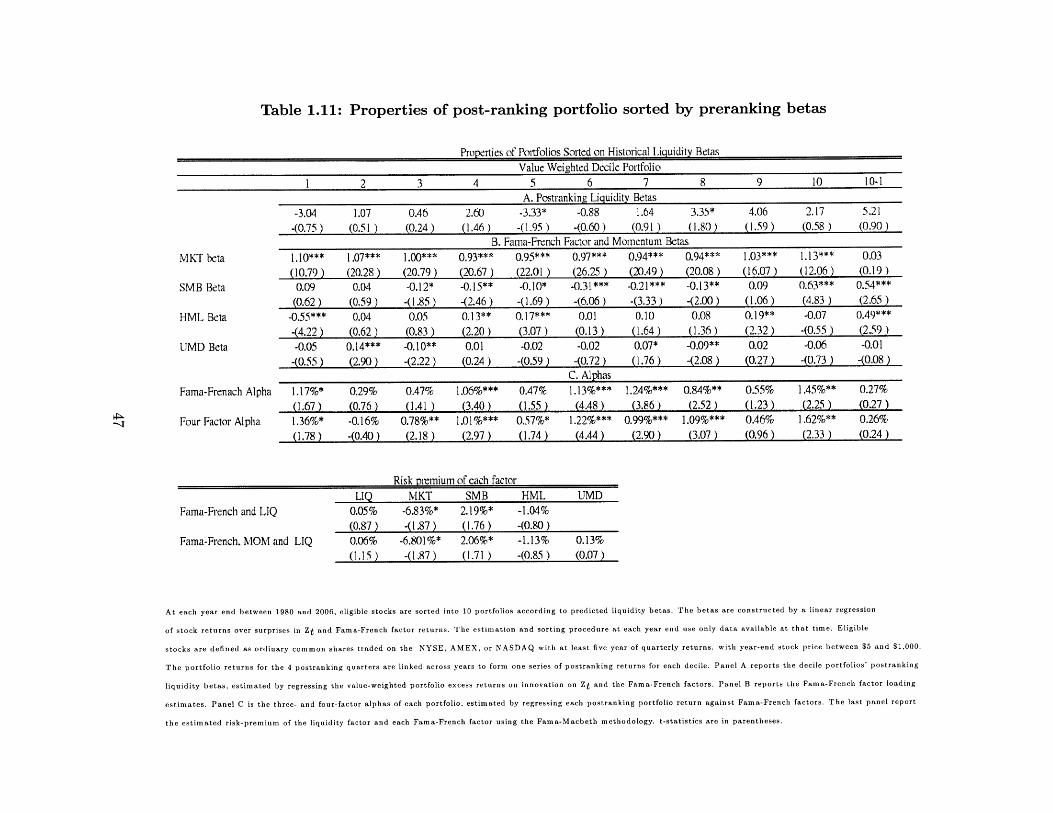
Table 1.11: Properties of post-ranking portfolio sorted by preranking betas

Properties of Portfolios Sorted on Historical Liquidity BetasValue Wei2hted Decile Portfolio

1 2 3 4 5 6 7 8 9 10 10-1A Pot$rankino I Licuidit Rets

MKT beta

SMB Beta

HML Beta

UMD Beta

Fama-Frenach Alpha

Four Factor Alpha

-3.04 1.07 0.46 2.60 -3.33* -0.88 1.64 3.35* 4.06 2.17 5.21-(0.75) (0.51) (0.24) (1.46) -(1.95) -(0.60 ) (0.91) (1.80) (1.59) (0.58) (0.90)

B. Fama-French Factor and Momentum Betas1.10*** 1.07** 1.00'** 0.93*** 0.95*** 0.97*** 0.94*** 0.94*** 1.03*** 1.13*** 0.03

(10.79) (20.28) (20.79) (20.67) (22.01) (26.25 ) (20.49) (20.08) (16.07) (12.06) (0.19)0.09 0.04 -0.12* -0.15** -0.10* -0.31*** -0.21*** -0.13** 0.09 0.63*** 0.54***

(0.62) (0.59) -(1.85 ) -(2.46) -(1.69) -(6.06) -(3.33) -(2.00) (1.06) (4.83) (2.65)-0.55*** 0.04 0.05 0.13** 0.17*** 0.01 0.10 0.08 0.19** -0.07 0.49***

-(4.22) (0.62) (0.83) (2.20) (3.07) (0.13) (1.64) (1.36) (2.32) -(0.55 ) (2.59)

-0.05 0.14*** -0.10** 0.01 -0.02 -0.02 0.07* -0.09** 0.02 -0.06 -0.01

-(0.55) (2.90) -(2.22) (0.24) -(0.59) -(0.72) (1.76) -(2.08) (0.27) -(0.73) -(0.08)C. Alphas

1.17%* 0.29% 0.47% 1.06%*** 0.47% 1.13%*** 1.24%*** 0.84%** 0.55% 1.45%** 0.27%

(1.67) (0.76) (1.41) (3.40) (1.55) (4.48) (3.86) (2.52) (1.23) (2.25) (0.27)

1.36%* -0.16% 0.78%** 1.01%*** 0.57%* 1.22%*** 0.99%*** 1.09%*** 0.46% 1.62%** 0.26%

(1.78) -(0.40) (2.18) (2.97) (1.74) (4.44) (2.90) (3.07) (0.96) (2.33) (0.24)

Fama-French and LIQ

Fama-French. MOM and LIQ

LIQ0.05%(0.87)0.06%(1.15)

Risk premium of each factorMKT SMB

-6.83%* 2.19%*-(1.87) (1.76)

-6.801%* 2.06%*-(1.87) (1.71)

At each year end between 1980 and 2006, eligible stocks are sorted into 10 portfolios according to predicted liquidity betas. The betas are constructed by a linear regression

of stock returns over surprises in Zt and Fama-French factor returns. The estimation and sorting procedure at each year end use only data available at that time. Eligible

stocks are defined as ordinary common shares traded on the NYSE, AMEX, or NASDAQ with at least five year of quarterly returns. with year-end stock price between $5 and $1,000.

The portfolio returns for the 4 postranking quarters are linked across years to form one series of postranking returns for each decile. Panel A reports the decile portfolios' postranking

liquidity betas, estimated by regressing the value-weighted portfolio excess returns on innovation on Zt and the Fama-French factors. Panel B reports the Fama-French factor loading

estimates. Panel C is the three- and four-factor alphas of each portfolio, estimated by regressing each postranking portfolio return against Fama-French factors. The last panel report

the estimated risk-premium of the liquidity factor and each Fama-French factor using the Fama-Macbeth methodology. t-statistics are in parentheses.

HML-1.04%-(0.80 )-1.13%-(0.85)

UMD

0.13%(0.07)

II

Table 1.12: Properties of post-ranking portfolio sorted by stock characteristics

Portfolios sorted by

Properties of Portfolios Sorted on Historical Liquidity Betas1 2 3 4 5 6 7 8 9 10 10-1

A. Postmankine Liouiditv BetasDollar Volume

Price

Illiquidity Ratio

Share Outstanding

Size

Volatility

Turnover

Share Volume

Portfolios sorted by

Dollar Volume

Price

Illiquidity Ratio

Share Outstanding

Size

Volatility

Turnover

Share Volume

5.59 3.07 4.15 1.09 1.97(2.49) (1.40) (2.29) (0.73) (1.38)

1.52 1.42 0.79 1.36 -0.05(1.07) (1.01) (0.54 ) (0.98) -(0.10)

-5.64-(2.34)

1.80 -1.31 -2.08 -0.95 2.59 -0.98 -0.04 3.07 1.79 -0.07 -1.87(0.51) -(0.45) -(0.78) -(0.44) (1.30) -(0.49) -(0.02) (2.12) (1.26) -(0.09) -(0.50)0.04 0.10 0.32 0.08 2.02 3.11 1.61 2.39 5.40 4.11 4.07

(0.06) (0.08) (0.27) (0.06) (1.63) (2.10) (1.04) (1.42) (2.46) (1.76) (1.64)4.31 3.46 2.90 1.80 0.87 1.74 -0.04 0.57 -0.29 0.23 -4.08

(1.91) (1.72) (1.65) (1.31) (0.66) (1.29) -(0.03) (0.41) -(0.24) (0.42) -(1.73)4.93 4.67 2.00 2.14 0.86 2.12 0.52 1.58 0.03 0.19 -4.74

(2.07) (2.33) (1.16) (1.32) (0.58) (1.47) (0.41) (1.11) (0.03) (0.37) -(1.90)-1.29 0.11 3.95 2.90 2.41 -1.11 0.60 -3.18 -6.00 -7.27 -5.98

-0.61 ) (0.07) (2.33) (1.61) (1.32) -(0.64 ) (0.28) -(1.26) -(1.69 ) -(1.47 ) -(0.04)0.85 0.02 -1.01 3.23 2.15 2.12 2.58 2.19 -3.05 -6.60 -7.45

(0.45) (0.01) -(0.55) (1.79) (1.18) (1.67) (1.52) (1.06) -(1.43) -(1.89) -(1.60)1.57 3.63 2.55 2.50 2.43 1.34 2.15 0.94 1.55 -0.27 -1.84

(0.71) (1.77) (1.38) (1.33) (1.42) (0.91) (1.53) (0.66) (1.09) -(0.45) -(0.76)B. Four Factor Alphas

1 2 3 4 5 6 7 8 9 10 10-11.60% 1.80% 1.10% 1.20% 0.90% 0.70% 0.70% 0.70% 0.50% 1.10% -0.50%(3.62) (4.11 ) (3.02) (4.18) (3.36) (2.38) (2.54) (2.30) (2.02) (11.01 ) -(1.02)-0.20% 0.80% 1.40% 1.00%, 1.20% 1.20% 0.90% 0.50% 1.20% 0.90% - 1.10%-(0.25) (1.41) (2.71 ) (2.34) (3.02) (3.23) (2.32) (1.76) (4.25) (6.24) (1.47)1.10%, 0.70% 0.60% 0.60%, 0.70% 1.00% 1.20% 1.40% 1.20% 1.60% 0.50%(9.98) (2.88) (2.68) (2.29) (2.77) (3.35) (3.96) (4.28) (2.73) (3.59) (1.07)1.80% 1.50% 1.20% 0.90% 1.00% 1.30% 0.80% 0.80% 0.70% 1.10% -0.70%(4.15) (3.70) (3.52) (3.24) (4.07) (4.98) (3.01) (2.96) (3.04) (10.32) -(1.58)1.30% 0.90% 1.00% 1.10% 0.90% 1.10% 1.00% 0.80% 0.90% 1.10% -0.20%(2.70) (2.34) (2.88) (3.40) (3.01) (3.77) (3.89) (2.99) (4.03) (10.73) -(0.39)1.20% 1.00% 0.60% 1.00% 1.30% 0.90% 0.50% 0.80% 1.20% 0.00% -1.20%(2.89) (3.06) (1.82) (2.78) (3.78) (2.79) (1.10) (1.53) (1.68) -(0.05) -(1.10)1.10% 1.10% 1.30% 0.70% 0.80% 1.20% 0.50% 1.60% 1.1 0% 1.70% 0.60%

(3.07) (2.52) (3.60) (2.01) (2.19) (4.83) (1.55) (3.88) (2.69) (2.45) (0.62)1.80% 1.20% 1.50% 1.30% ,0.90% 0.90% 0.50% 0.70% 0.60% 1.10% -0.70%

(4.23) (2.89) (4.07) (3.55) (2.66) (3.08) (1.99) (2.53) (2.29) (9.74) -(1.47 )

See notes to Table 1.11. Panel A shows the postranking liquidity beta when the portfolio are sorted by stock characteristics. The betas are

estimated as the slopes from the regression of excess portfolio postranking returns on Fama french factor, momentum and innovation in

liquidity. Panel B reports report each decile portfolio's postranking alphas. The alphas are estimated as intercepts from the regression

of excess portfolio postranking returns on Fama-French factors and momentum. The t-statsitics are in parentheses

Table 1.13: Risk premium of postranking portfolios sorted by stock characteristicsRisk premium of each factor

Portfolios sorted by: LIQ MKT SMB HML UMD

Dollar Volume

Illiquidity Ratio

Size

Share Outstanding

Price

Volatility

Turnover

Share Volume

Four Traded Factors -0. 17%* -3.77%** 0.66% 0.86%

-(1.94) -(2.45 ) (0.82) (0.55)Five Traded Factors -0. 14%* -2.45% 0.37% 0.56% 5.28%*

-(1.65 ) -(1.63) (0.46) (0.35) (1.76)Four Traded Factors -0.11%* -1.87% 0.02% 3.33%**

-(1.74) -(1.25) (0.03) (2.36)Five Traded Factors -0.05% -1.79% 0.03% 1.82% 2.66%

-(0.75) -(1.19) (0.04) (1.00) (0.66)Four Traded Factors 0.04% -0.66% 0.49% 0.38%

(0.65) -(0.34) (0.83 ) (0.29)Five Traded Factors 0.03% -1.70% 0.52% 0.28% -1.32%

(0.42) -(0.49 ) (0.88) (0.21) -(0.36)Four Traded Factors 0.23%* 0.23% 0.37% 0.57%

(1.87) (0.14) (0.68) (0.59)Five Traded Factors 0.24% 0.43% 0.32% 0.53% 1.02%

(1.60) (0.22) (0.52) (0.50) (0.35)Four Traded Factors -0.11%* 0.38% -0.98% 1.83%*

-(1.73) 0.15 ) -(1.52) (1.78)Five Traded Factors -0.11%* 1.03% -0.64% 2.42%** 0.7%

-(1.74) (0.41 ) -(0.85) (2.06) (0.37)Four Traded Factors 0.04% -1.80% -0.70% -1.05%

(0.74) -(0.99) -(0.39) -(0.75)Five Traded Factors 0.01% 0.89% 2.53% 3.36% 5.39%***

(0.27) (0.49) (1.13) (1.64) (2.79)Four Traded Factors -0.03% -0.96% 0.28% -0.07%

-(0.49) -(0.72) (0.39) -(0.07)Five Traded Factors 0.00% -0.79% 0.41% -0.15% 2.02%

(0.06) -(0.60) (0.55) -(0.15) (0.98)Four Traded Factors -0.13%* -1.00% 0.82% 1.65%

-(1.71) -(0.73 ) (1.06) (1.14)Five Traded Factors -0.03% -0.98% 0.88% 1.73% -5.27%*

-(0.35) -(0.72) (1.13) (1.20) -(1.78)

See notes to Table 1.11. This table reports the risk premium associated with the liquidity factor, with the portfolios being sorted by

stock characteristics. The premium is reported as monthly values. The t-statistics are in parentheses.

Table 1.14: Properties of postranking portfolios sorted by predicted liquidityPropertics of Pornolios Sorted on Predicted Liquidity Betas

0.21(0.44 )

MNKTS L 10O**

(77.26 )SMB Beta -0.22"

-12.01 )HML Beta -0.06

"-"

-.94 1

Fama-Frnncch Alpha 1.17%*(.67 )

Fama-French and LIQ

Fama-French, MOM and LIQ

0.90

(0.62)

1.02"*

(27.11 )0.15""

(2.89)

(7.62 )

0.29%(0.76 )

0.83(0.54 )

0.98**(24.78 )0.37* *

(6.49 )0.33"-

(6.61)

0.47%(1.41 1

4

0.96

(0.67)B.

0.96"**

(25.65 )0.44'"**(6s.25 )

0.37'**(7.93

1.06%* 11.0

Value Weighted Dkcile Portnfolio5 6 7 8

A. Postranking Liquidity Betas

1.09 1.99 0.38 2.62

(0.77) (1.39) (0.28 1.58)

Fama-French Factor and Mommumn Betas0.96"' 0.89"* 0.86

** 0.75***

(26.01) (24.01 ) (23.71 ) (16.45 )0.55

**" 0.68* 0.73** 0.73-

*

(10t.) (1289) (14.18 ) (1120)0.43

* 0.4"

*' 0.48"** 0.55"*

(9.33 (9.51 ) (10.52 ) (9.56C. Alphas

0.47% 1.13%*'* 1.24%*** 0.84%"

(155 ) (4.1 ) (3.6 ) ,2.52 1

9

3.12(1.57 )

0.63'**

(12.83

(9.70)0.51

* "

(8.28)

0.55%(13)

10

4.27"*

(2.33 )

0.56...(11.33 )

0.51"

0.44...(7.02 )

1.45%-1

(2) i

0-1I

4.07"(2.14)

-0.44**

-18.27 )0.76"*

(0.21 )0.50"

*

(7.60 )

0.27%(02.7

Risk pmium of each factor

LIQ MKT SMB HML UMD

0.15% -3.04%** -0.02% 0.90%

-(1.64) -(1.99) (0.03) (0.77)-0.15% -2.52%* 0.04% 0.42% 2.94%

-(1.64 ) i(1.76) (0.05) (0.29) (0.57

See notes to Table 1.11. Panel A reports the decile portfolios' postranking liquidity betas, estimated by regressing the value-weighted portfolio excess returns on

innovation on Zt and the Fama-French factors. Panel B reports the Fama-French factor loading estimates. Panel C is the three- and four-factor alphas of each

portfolio, estimated by regressing each postranking portfolio return against Fama-French factors. The last panel report the estimated risk-premium of the liquidity

factor and each Fama-French factor using the Fama-Macbeth methodology. t-statistics are in parentheses.

. 67 1 .(0761 il 2 (225

III

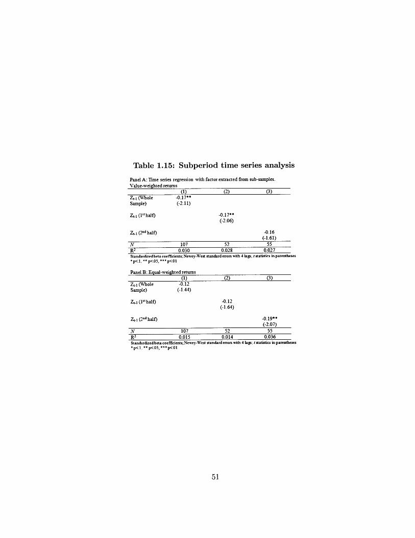
Table 1.15: Subperiod time series analysis

Panel A: Time series regression with factor extracted from sub-samples.

Value-weighted returns(1) (2) (3)

Zt-. (Whole -0.17**Sample) (-2.11)

At- (P t half) -0.17**

(-2.06)

Zt. (2-d half) -0.16

(-1.61)

N 107 52 55R2 0.030 0.028 0.027

Standardizedbeta coefficents;Newey-West standard errors ith 4 lags; t statistics in parentheses*p<.l, **p<.05, ***p<.01

Panel B: Equal-weighted returns

(1) (2) (3)Zl- (Whole -0.12

Sample) (-1.44)

t- (I't half) -0.12(-1.64)

A-t1 (2d half) -0.19**(-2.07)

N 107 52 55R

2 0.015 0.014 0.036Standardizedbeta coefficients;Newey-West standard errors with 4 lags; t statistics in parentheses*p<.l ** p<OS, ***p<01

Bibliography

[1] Y. Amihud. Illiquidity and stock returns: Cross-section and time-series effects.

Journal of Financial Markets, 5(1):p31 - 56, 2002.

[2] Y. Amihud and H. Mendelson. Asset pricing and the bid-ask spread. Journal of

Financial Economics, 17(2):p223 - 249, 1986.

[3] D. Avramov and R. Wermers. Investing in mutual funds when returns are pre-

dictable. Journal of Financial Economics, 81:339-377, 2006.

[4] S. G. Badrinath and S. Wahal. Momentum trading by institutions. The Journal of

Finance, 57(6):2449-2478, 2002.

[5] J. B. Berk and I. Tonks. Return persistence and fund flows in the worst performing

mutual funds. Working Paper, 2007.

[6] M. Bolding and B. Ding. User's guide to thomson reuters mutual fund and invest-

ment company common stock holdings databases on wrds. 2008.

[7] M. J. Brennan, T. Chordia, and A. Subrahmanyam. Alternative factor specifications,

security characteristics, and the cross-section of expected stock returns. Journal of

Financial Economics, 49(3):p345 - 373, 1998.

[8] M. J. Brennan and A. Subrahmanyam. Market microstructure and asset pricing: On

the compensation for illiquidity in stock returns. Journal of Financial Economics,

41(3):p441 - 464, 1996.

[9] S. Brown and W. N. Goetzmann. Performance persistence. Journal of Finance,

50:679-698, 1995.

[10] T. R. Burch and B. Swaminathan. Are Institutions Momentum Traders? SSRN

eLibrary, 2001.

[11] M. M. Cahart. On persistence in mutual fund performance. Journal of Finance,

52:57-82, 1997.

[12] J. Y. Campbell, S. J. Grossman, and J. Wang. Trading volume and serial correlation

in stock returns. Quarterly Journal of Economics, 108(4):p905 - 939, 1993.

[13] A. S. Chordia, Tarun and A. Subrahmanyam. Liquidity dynamics and cross-

autocorrelations. Working Paper, 2005.

[14] J. D. C. Cohen, Randolph and L. Pastor. Judging fund managers by the company

that they keep. Journal of Finance, 60:1057-1096, 2005.

[15] G. Connor and R. A. Korajczyk. Performance measurement with the arbitrage

pricing theory: A new framework for analysis. Journal of Financial Economics,

15:373-394, 1986.

[16] G. Connor and R. A. Korajczyk. Roisk and return in an equilibrium apt: Application

of a new test methodology. Journal of Financial Economics, 21:255-289, 1988.

[17] J. Coval and E. Stafford. Asset fire sales (and purchases) in equity markets. Journal

of Financial Economics, 86(2):479-512, 2007.

[18] V. T. Datar, N. Y. Naik, and R. Radcliffe. Liquidity and stock returns: An alter-

native test. Journal of Financial Markets, 1(2):203-219, 1998.

[19] J. L. Davis, E. F. Fama, and K. R. French. Characteristics, covariances, and average

returns: 1929 to 1997. Journal of Finance, 55(1):p389 - 406, 2000.

[20] G. Duffie. Trading volume and return reversals. Finance and Economics Discussion

Paper Series, (192), 1992.

[21] E. F. Fama and K. R. French. Common risk factors in the returns on stock and

bonds. Journal of Financial Economics, 33(1):p3 - 56, 1993.

[22] E. F. Fama and K. R. French. Multifactor explanations of asset pricing anomalies.

Journal of Finance, 51(1):p55 - 84, 1996.

[23] E. F. Fama and D. M. James. Risk, return and equilibrium: Empirical tests. Journal

of Political Economy, 81:607-636, 197.

[24] A. Frazzini and 0. A. Lamont. Dumb money: Mutual fund flows and the cross-

section of stock returns. Journal of Financial Economics, 88(2):299 - 322, 2008.

[25] A. R. Gallant, P. E. Rossi, and G. Tauchen. Stock prices and volume. The Review

of Financial Studies, 5(2):199-242, 1992.

[26] M. Grinblatt and S. Titman. Mutual fund performance: An analysis of quarterly

portfolio holdings. Journal of Business, 62:393-416, 1989.

[27] M. Grinblatt and S. Titman. Performance measurement without benchmarks: An

examination of mutual fund returns. Journal of Business, 66:47-68, 1993.

[28] S. T. Grinblatt, Mark and R. Wermers. Momentum investment strategies, portfolio

performance, and herding: A study of mutual fund behavior. American Economic

Reivew, 85:1088-1105, 1995.

[29] S. Grossman and M. Miller. Liquidity and market structure. Journal of Finance,

43(3):617-633, 1988.

[30] N. Jegadeesh and S. Titman. Returns to buying winners and selling losers: Impli-

cations for stock market efficiency. Journal of Finance, 48(1):65-91, 1993.

[31] C. S. Kacperczyk, Marcin and L. Zheng. On the industry concentration of actively

managed equity mutual funds. Journal of Finance, 60:1983-2012, 2005.

[32] A. S. Kyle. Continuous auctions and insider trading. Econometrica, 53(6):1315-

1335, 1985.

[33] C. M. C. Lee and B. Swaminathan. Price momentum and trading volume. Journal

of Finance, 55(5):2017-2069, 2000.

[34] G. Llorente, R. Michaely, G. Saar, and J. Wang. Dynamic volume-return relation

of individual stocks. Review of Financial Studies, 15(4):1005-1047, 2002.

[35] R. M. G. S. Llorente, Guillermo and J. Wang. Dynamic volume-return relations of

individual stocks. Review of Financial Studies, 15:1005-1047, 2002.

[36] A. W. Lo, H. Mamaysky, and J. Wang. Asset prices and trading volume under fixed

transactions costs. Asset Prices and Trading Volume under Fixed Transaction Vosts,

2001.

[37] A. W. Lo and J. Wang. Trading volume: Definitions, data analysis, and implications

of portfolio theory. Review of Financial Studies, 13(2):p257 - 300, 2000.

[38] A. W. Lo and J. Wang. Trading volume: Implications of an intertemporal capital

asset pricing model. Journal of Finance, 61(6):p2805 - 2840, 2006.

[39] R. Lowenstein. When genius failed: The rise and fall of long-term capital manage-

ment. 2000.

[40] M. S. Mamasky, Harry and H. Zhang. Estimating the dynamics of mutual fund

alphas and betas. Review of Financial Studies, 21(1):223-264, 2008.

[41] H. Mamaysky, M. Spiegel, and H. Zhang. Estimating the dynamics of mutual fund

alphas and betas. Review of Financial Studies, 21(1):233-264, January 2008.

[42] R. C. Merton. Optimum consumption and portfolio rules in a continuous-time model.

Journal of Economic Theory, 3(4):373 413, 1971.

[43] R. C. Merton. An intertemporal capital asset pricing model. Econometrica,

41(5):867-887, 1973.

[44] L. Pastor and R. F. Stambaugh. Liquidity risk and expected stock returns. Journal

of Political Economy, 111(3):p642 - 685, 2003.

[45] A. Petajisto. The Index Premium and its Hidden Cost for Index Funds.

eLibrary, 2008.

[46] J. Shanken. Intertemporal asset pricing: An empirical investigation.

Econometrics, 45:99-120, 1990.

[47] W. Sharpe. Asset allocation: Management style and performance measure- ment.

Journal of Portfolio Management, pages 7-19, 1992.

[48] R. W. Sias. Reconcilable Differences: Momentum Trading By Institutions.

Financial Review, Vol. 42, No. 1, pp. 1-22, February 2007.

[49] R. W. Sias. Institutional herding. The Review of Financial Studies, 17(1):165-206,

2004.

[50] D. Vayanos. Transaction costs and asset prices: A dynamic equilibrium model.

Review of Financial Studies, 11(1):1-58, 1998.

[51] J. Wang. A model of competitive stock trading volume. Journal of Political Econ-

omy, 102:127-167, 1994.

[52] R. Wermers. Momentum investment strategies of mutual funds, performance per-

sistence, and survivorship bias. Working Paper, 1997.

SSRN

Journal of

The