MPRAMunich Personal RePEc Archive

Choice of Crops and EmploymentUncertainty in the Off-farm LaborMarket

Syed Naimul Wadood and Russell L. Lamb

Department of Economics, North South University, Dhaka,Bangladesh

20. July 2006

Online at http://mpra.ub.uni-muenchen.de/10779/MPRA Paper No. 10779, posted 28. September 2008 00:05 UTC

Choice of Crops and Employment Uncertainty in the Off-Farm Labor Market

Syed N. Wadooda,*, Russell L. Lambb

a Assistant Professor, Department of Economics, North South University,12 Banani C/A, Kemal Ataturk Avenue,

Dhaka-1213, Bangladesh b Associate Director, Navigant Consulting, Inc., 1801 K Street, NW, Washington DC 20006, USA

Abstract Cultivator households in some developing areas use off-farm labor supply as an insurance against crop income shocks, whilst employment is uncertain in this off-farm labor market. This paper hypothesizes that, given limited opportunities for ex post consumption smoothing, employment uncertainty influences risk-averse households’ crop choice decisions-- they would opt for more conservative crop choices in case they expect unfavorable supply opportunities in the labor market. A two-period stochastic dynamic programming model is developed. A panel data set from the ICRISAT survey of the semi-arid tropics of India is examined. Estimation is based on random effects and fixed effects Tobit specifications. Estimation results indicate statistically significant impact of household expectation of harvesting period male unemployment rates on ex ante crop choices. Results also indicate strong influence of household irrigated land share on crop choices. JEL Classification. O1 Keywords. Crop Choice; Off-farm Labor Market; Risk; Panel Data

1. Introduction

Risk factors, such as weather risk, influence cultivators’ choices of crops. This is due to absence

of a complete set of markets in developing country agricultural sector (Kurosaki (1998)). A competitive

equilibrium is considered Pareto-optimal if the set of markets, including insurance markets against risk, is

complete (Debreu (1959); Arrow (1964)). There is “separability” between production decisions taken by

households and their risk and consumption preferences in that case (Singh, Squire and Strauss (1986);

Bardhan and Udry (1999)). Since a complete set of markets does not exist in developing country

agricultural sector-- this “separability” is absent and thereby risk considerations influence households’

production decisions (Antle (1983); Roe and Graham-Tomasi (1986)).

* Corresponding Author. Tel: +88-02-9885611~20 (Ext. 217); Fax: +88-02-8823030 Email address: nwadood@northsouth.edu (Syed N. Wadood)

Apart from crop production, one important source of income for cultivator households,

particularly small and medium farmers, in many areas of developing countries is participation in the off-

farm labor market (Kochar (1999); Lamb (2003)). In the semi-arid areas of India, as it is documented in

the ICRISAT survey, the off-farm labor market had a two-tier structure (Walker and Ryan (1990)). On

one tier were the daily “casual” laborers while on another tier were the “permanent” laborers who were

hired in advance for multiple periods of time at a fixed wage rate. The major portion of off-farm labor

income was earned in the form of “casual” labor, especially in the daily off-farm wage labor market.

Employees had freedom to choose among different employers. Contracts were typically negotiated for a

short period, usually a single day or two, and payment was made each day for an agreed number of hours.

As long as labor market and own-farm productivity are not perfectly correlated, it is possible for

households to use market labor supply as one means to cope with risk in own-farm crop production (Rose

(2001)). Yet the off-farm labor market is not without its own aspects of uncertainty -- employment is

uncertain in this market at any point in time. To the extent that a major portion of labor demanded in this

off-farm labor market is agricultural, realizations of weather conditions play a role in contributing to

uncertainty in this market, by partly influencing wage rates and unemployment rates. If weather shocks

turn out to be positive, cultivators will have a higher output in the harvest season, which implies that their

demand for own-farm labor will be higher. Since they will need to hire any excess demand of own-farm

labor in their farms over and above their own family labor supply, this translates into a higher demand for

off-farm labor. To the extent that changes in the supply of labor lags behind increases in the demand for

labor in the village off-farm labor market, wage rates for labor in that market will tend to increase and

likewise labor unemployment rates will tend to decrease. The reverse will tend to happen in case of

negative realizations of rainfall shocks.

The testable hypothesis of this paper is that uncertainty of off-farm labor income influences crop

choice decisions. Assuming ex post risk-coping mechanisms (i.e., credit, borrowing or transfers) are

unavailable to households and they are to choose crops from among different output risk distributions--

we hypothesize that they would rather choose crops with lower output risks in the face of their

2

expectation of a higher employment uncertainty in the off-farm labor market. One can consider this as a

form of conservative ex ante risk-management strategy given unfavorable expectations of future off-farm

labor income earnings.

The literature recognizes the role of off-farm labor supply as an insurance against crop income

shocks (see Rose (1993), (2001); Kanwar (1999); Kochar (1999); Lamb (2003)). Our paper is a

continuation of the literature with a focus on the plausible relationship between employment uncertainty

in the off-farm labor market and the ex ante crop choice decisions. Among the literature, Rose (1993) is a

study of the ex ante effect of the riskiness of distribution of rainfall as well as the ex post effects of

weather shocks on the labor supply decisions of cultivator households. Households facing greater

dispersion in rainfall allocate less labor towards risky own-farm production and more labor to the less

risky alternative activity--the off-farm labor market. Also in periods of bad weather and low rainfall

households partially compensate for shortfalls in own-firm production income through work in the labor

market. Kochar (1999) focuses on the responsiveness of the market hours of work of cultivator

households to idiosyncratic or household-specific shocks to crop income. Household males increase their

market hours of work in response to unanticipated variations in crop profits. Conditional on hours of

work, crop income shocks have negative effects on consumption, confirming that household ability to

protect its’ consumption from crop income shocks depends, in most parts, on its’ adjustments in hours of

work. Kanwar (1999) is one paper that mentions employment risk in the off-farm labor market. This

focuses on whether a decrease in revenue uncertainty (in crop income) will affect off-farm labor supply

and finds that since production risks are carried forward into the local labor market, households might not

be able to use the labor market as a hedge against production risk. Lamb (2003) develops a two period

model in which a risk-averse cultivator household uses off-farm labor supply to mitigate the effects of

production shocks ex post, which leads to more efficient ex ante production choices in the presence of

production risk, i.e., greater use of chemical fertilizers. Controlling for exogenous weather risk, this paper

positively relates fertilizer use with the “depth” of the off-farm labor market.

3

We develop a two period dynamic stochastic model to show that under particular conditions, risk-

averse households’ expectations of a lower (higher) “depth”1 or a lower (higher) wage rate in the off-farm

labor market in the next period would lead them to allocate a higher (lower) proportion of their cultivable

land to crops with safer returns-- a lower (higher) share of irrigated land also leads to a higher (lower)

land share being allocated to crops with safer returns. A panel data set of cultivator households from the

ICRISAT survey of the semi-arid areas of India is examined. Fixed effects and random effects Tobit

regressions for estimating household land share as well as fixed effects and random effects regressions of

differences of household land shares and that of crop returns have been used. The results indicate

statistically significant impacts of household expectation of harvest period male unemployment rates in

the off-farm labor market on crop choices, taking the planting period male unemployment rates as proxy.

They also indicate statistically significant impacts of household irrigated land share on crop choices and

land shares.

The paper is organized as follows. The next section develops a conceptual framework. After

discussing data and estimation techniques in the following two sections, Sections 3 and 4 respectively,

empirical results are presented in Section 5. Some concluding remarks are presented in the final section.

2. Conceptual Framework

2.A. Model Specification

The cultivator household is assumed to be an expected utility maximizer and it maximizes

expected utility of income EU(I), where I is income, with U′(I)>0 and U′′(I)<0-- it is risk averse. Savings

is absent and current consumption is equivalent to current income.

There is a single agricultural crop season in the year and there are two decision points in that

season, t1 and t2, each one preceding one period, period 1 (planting) and period 2 (harvesting), 1 The “depth” of the off-farm labor market can be measured in two different ways. The labor market can be considered “deeper” or in other words more “diversified”, the higher the share of non-agricultural labor in total labor demanded in that market, since that will indicate the market has a higher number of alternative sources of labor demand instead of being fully dependent on agriculture as the only source of demand. Another interpretation of the depth of the labor market could be based on its unemployment rate-- the lower the unemployment rate in that market the “deeper” or, in other words, the more vibrant is the labor market (Lamb (2003: 263)).

4

respectively. The household has two sources of income-- own-farm income from crop production and off-

farm labor income from the village daily casual wage labor market. This model does not allow for credit,

borrowing, remittances or transfers. The household has a fixed amount of cultivable land (set to unity)

and has to distribute this land between two crops-- crop 1 and crop 2. Crop 1 is characterized by low mean

and low variance of returns as well as less susceptibility to realizations of rainfall shocks. Crop 2 has high

mean and high variance of returns and is more susceptible to realizations of rainfall shocks. The

household has a portfolio selection problem-- a larger allocation of land to crop 2 at the expense of crop 1

exposes it more towards realizations of rainfall shocks whereas a smaller allocation of land to crop 2

reduces its exposure. At time t1, the start of the planting period, the household decides on land allocation

between crops 1 and 2. This crop choice decision is measured by the term k-- defined as the proportion of

one unit of cultivable land allocated to the safer crop 1 (0≤ k ≤ 1); and the rest (1– k) to crop 2. In between

two decision points, t1 and t2, the rainfall shock γ is resolved, measured as difference between the actual

rainfall and the expected rainfall and it is independently and identically distributed of zero mean and unity

variance. At time t2, the start of the harvest period, the household decides on allocation of harvest period

family labor to crops 1 and 2. Consumption is assumed to take place only in period 2.

Crop production functions have been specified as (following Just and Pope (1978))2:

Crop 1: Q1 = f (1) (k, L1) + h(1)( k, L1)γ

Crop 2: Q2 = f (2) (1 – k, L2) + h(2)(1 – k, L2)γ

E(γ)= 0; Var(γ)= 1

h(1)( k, L1), h(2)(1 – k, L2) >0.

Here, Q1 is the output function of crop 1, which consists of the deterministic component, f (1)(k,

L1), which relates inputs to mean output of the crop and a stochastic component, h(1)(k,L1)γ, which relates

inputs to the variance of output of that crop. Q2 is the corresponding expression for crop 2. The inputs are

2 Specification here is a simple restatement of a standard multiplicative random effects specification of random crop outputs common in literature. A conventional multiplicative random effect enters into a random production function in the following

form: Q=θf(x) where Q is a random crop output and x is input while θ is a random term with meanθ . Defining γ ≡ θ −θ , h(x)

≡ f(x) and y(x) ≡ θ f(x) one can obtain Q= y(x) + γh(x). This is the Just and Pope (1978) specification (Feder (1980: 266)).

5

the share of cultivable land and harvest period labor allocated to the crop in question; these inputs are

assumed gross complements in production. The randomness in crop outputs is contributed by the rainfall

shock γ with mean zero and variance unity. This shock affects two crops differently, captured by the term

h(1)( k, L1) in the case of crop 1 and h(2)(1 – k, L2) in the case of crop 2.

The household knows the means and variances of the crops and their relative magnitudes-- E(Q1)

= f (1) ( k, L1), E(Q2) = f (2)( – k, L2),Var(Q1) = [h(1)( k, L1)]2 and Var(Q2)= [h(2)(1 – k, L2)]2. By assumption,

E[Q1( k , 1L )] < E[Q2 ( k , 1L )] and Var Q1( k , 1L ) < Var Q2( k , 1L ).

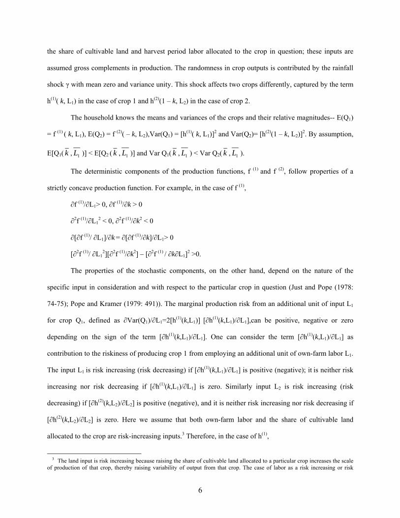
The deterministic components of the production functions, f (1) and f (2), follow properties of a

strictly concave production function. For example, in the case of f (1),

∂f (1)/∂L1> 0, ∂f (1)/∂k > 0

∂2f (1)/∂L12 < 0, ∂2f (1)/∂k2 < 0

∂[∂f (1)/ ∂L1]/∂k = ∂[∂f (1)/∂k]/∂L1> 0

[∂2f (1)/ ∂L12][∂2f (1)/∂k2] – [∂2f (1) / ∂k∂L1]2 >0.

The properties of the stochastic components, on the other hand, depend on the nature of the

specific input in consideration and with respect to the particular crop in question (Just and Pope (1978:

74-75); Pope and Kramer (1979: 491)). The marginal production risk from an additional unit of input L1

for crop Q1, defined as ∂Var(Q1)/∂L1=2[h(1)(k,L1)] [∂h(1)(k,L1)/∂L1],can be positive, negative or zero

depending on the sign of the term [∂h(1)(k,L1)/∂L1]. One can consider the term [∂h(1)(k,L1)/∂L1] as

contribution to the riskiness of producing crop 1 from employing an additional unit of own-farm labor L1.

The input L1 is risk increasing (risk decreasing) if [∂h(1)(k,L1)/∂L1] is positive (negative); it is neither risk

increasing nor risk decreasing if [∂h(1)(k,L1)/∂L1] is zero. Similarly input L2 is risk increasing (risk

decreasing) if [∂h(2)(k,L2)/∂L2] is positive (negative), and it is neither risk increasing nor risk decreasing if

[∂h(2)(k,L2)/∂L2] is zero. Here we assume that both own-farm labor and the share of cultivable land

allocated to the crop are risk-increasing inputs.3 Therefore, in the case of h(1),

3 The land input is risk increasing because raising the share of cultivable land allocated to a particular crop increases the scale of production of that crop, thereby raising variability of output from that crop. The case of labor as a risk increasing or risk

6

∂h(1)/∂L1> 0, ∂h(1)/∂k > 0

∂2h(1)/∂L12 < 0, ∂2h(1)/∂k2 < 0

∂[∂h(1)/∂L1]/∂k = ∂[∂h(1)/∂k]/∂L1> 0.

The second consideration is period 2 output price terms. These are specified as:

price of crop 1: p1

price of crop 2: p2.

-- p1 is the expected period 2 price of crop 1 and p2 is the expected period 2 price of crop 2. Prices

are assumed exogenously determined, implying zero impact of local weather variations on prices,

assuming crop output markets are regionally integrated. Prices are assumed “correctly” forecast.

The third consideration is the wage rate in the village off-farm labor market. Wage rate is

hypothesized to be positively affected by shocks in rainfall-- high wage rates are caused by, among other

factors, positive realizations of rainfall shocks whilst low wage rates are caused by, among other factors,

negative realizations of the same4. It is possible to specify harvest period labor market wage rates as

functions of realizations of rainfall shocks, such as this linear function,

WK = kw + (1– dk)γ (0 ≤ dk ≤ 1)

-- WK and kw are village-specific realized and expected period 2 wage rates, respectively. Here

dk is the “depth” of the village off-farm labor market that counteracts against the impact of shocks in

decreasing input, on the other hand, is not straightforward. It is possible to argue that labor is risk decreasing in the sense that a more intensive use of harvest period on-farm labor can help reduce the damage done to crop yield as a result of a negative rainfall shock. But, in the context of this particular model, harvest period on-farm labor is tied to the share of land allocation in a complementary way, i.e., a higher share of land allocation for a crop would lead to a higher amount of harvest period own-farm labor needed for that crop. Since land allocation is a risk-increasing input, labor is also considered risk increasing. 4 There could be particular institutional factors involved which might prevent the wage rate from reaching exactly a market-clearing level-- once unemployment exists at the initial wage rate this may still persist at the new wage rate after the shock. Since the wage rate at the labor market may move from one disequilibrium level to another-- it is difficult to understand the impact of rainfall shocks on the unemployment rate. One possible outcome is that the unemployment rate decreases as a result of positive rainfall shocks-- this can be caused by a sharp increase in labor demand unmatched by increases in labor supply in the market. One can consider the situation where wage rates in the off-farm labor market are not at the market-clearing rates and unemployment persists in the market at the going wage rates. This is the case for the off-farm labor markets in the semi-arid tropics region of India, where unemployment rates have been found to be positive in each of the survey years and at each of the villages. The unemployment rates are affected by seasonal variations, local crop-labor use as well as gender-based segmentation in that market (Walker and Ryan (1990: 122-124)).

7

rainfall (Lamb (2003:363)) -- therefore (1– dk) is a measure of the impact of the rainfall shock on the

realized wage rate. The mean value of the realized period 2 wage rate is kw and variance is (1– dk) 2.

The fourth consideration is of distribution of household family labor among competing demands

for it. The household is assumed to have a given total labor time, T, in period 2 that it allocates among

three alternative uses: on-farm family labor applied to crop 1 (L1), on-farm family labor applied to crop 2

(L2) and the residual time to daily wage labor in the off-farm labor market. We maintain the following

assumptions regarding household labor allocation and related considerations: (a) households consider

own- and off-farm labor as perfect substitutes, (b) households do not hire-in labor, (c) bullock labor used

(family-owned or hired-in) to crops 1 and 2 in period 1 are proportional to family on-farm labor applied to

crops, (d) the amount of fertilizer and insecticide applied to the crops is proportional to family own-farm

labor applied to the crops in period 1 and (e) leisure in period 2 is a fixed proportion of the total family

labor time available in period 2.

The testable hypothesis of this study is that cultivator households’ expectations regarding the off-

farm labor market at a later period influence its’ crop choice decisions. Under the testable hypothesis,

unfavorable household expectations regarding the off-farm labor market at a later period (i.e., a lower

depth or a lower wage rate) would tend to cause its’ ex ante crop choices to move towards less risky but

less profitable crops. Building on the testable hypothesis, the model has two particular focus questions,

(1) ∂ k/ ∂dk < 0 ?

(2) ∂ k/∂ kw < 0 ?

In the presence of a risk-mitigating factor (i.e., share of irrigated land, denoted by a) the

household can be more risk-taking in its approach to crop choices. We hypothesize that a higher share of

irrigated land would tend to decrease the household land share allocated to the less risky crops. So there is

one more focus question in the extended model-- (3) ∂ k/ ∂a < 0 ?

2.B. Maximization Problem

The households’ crop income and off-farm labor income in period 2 are,

8

Crop income ≡ p1Q1 + p2 Q2

= p1[f (1)( k, L1) + h(1)( k, L1)γ] + p2 [f (2) (1 – k, L2) + h(2)(1 – k, L2)γ]

Off-farm labor income ≡ [ kw + (1– dk)γ] [T – L1 – L2]

The household total income from crop production and off-farm labor supply is,

I = p1[f (1) ( k, L1) + h(1)( k, L1)γ] + p2 [f (2) (1 – k, L2) + h(2)(1 – k, L2)γ]

+ [ kw + (1– dk)γ] [T – L1 – L2] (1)

The household is assumed to use a two period dynamic programming algorithm to solve the

maximization problem (Intriligator (1971)). It solves a conditional second period problem first, choosing

the optimal allocation of labor between own-farm crop production and off-farm labor supply conditional

on its choice of value of the land allocation term (k) in the first period and realization of rainfall

uncertainty. Then it solves the first period problem, choosing the optimal value for the land allocation

term conditional on the responses of labor allocation in the second period to the choice of value of the

land allocation term (k) in the first period and realization of rainfall uncertainty.

2.C. The Second Period Problem

Following backward induction logic, we concentrate on the second period problem first. At the

start of period 2, t2, the rainfall uncertainty γ is resolved and value for the land allocation term k has

already been determined. Since there is no uncertainty at this point, the problem now is a simple

maximization problem conditional on the known realization of uncertainty and optimal decision taken in

the previous period. Let γ be the realized rainfall shock, resolved on or before time t2, and k* be the

optimal value of land allocation term chosen at time t1.

At time t2 the problem stands at,

Max I = p1[f (1)(k*,L1) + h(1)( k*,L1)γ]+p2 [f (2)(1– k*,L2) + h(2)(1 – k*,L2)γ]+[ kw + (1– dk)γ] [T – L1 – L2] L1, L2

The first order conditions for the second period problem are,

With respect to L1, ∂I /∂L1 = p1[∂f (1)(.)/∂L1 + [∂h(1)(.)/∂L1]γ] – [ kw + (1– dk)γ] = 0 (2)

9

With respect to L2, ∂I /∂L2 = p2 [∂f (2)(.)/∂L2 + [∂h(2)(.)/∂L2]γ] – [ kw + (1– dk)γ] = 0 (3)

Then, [value of marginal product of labor to crop 1]= [value of marginal product of labor to crop 2]=

[opportunity cost of labor in the off-farm labor market].

The second order conditions for the second period problem are,

With respect to L1, ∂2I /∂L12 = p1 [∂2f (1)(.)/∂L1

2 + [∂2h(1)(.)/∂L12]γ] < 0 (4)

With respect to L2, ∂2I /∂L22 = p2 [∂2f (2)(.)/∂L2

2 + [∂2h(2)(.)/∂L22]γ] < 0 (5)

The second order cross partial derivative terms are (derived from (2) or (3)),

∂2I /∂L1∂L2 = ∂I2 /∂L2∂L1 = 0 (6)

In expression (4) the term ∂2I/∂L12 is negative, since ∂2f(1)(.)/∂L1

2 and ∂2h(1)(.)/∂L12 are negative

following the previous discussions.5 Similarly the term ∂2I/∂L22 is negative.

The other second order condition of the second period problem is also shown to be satisfied,

[∂2I /∂L12] [∂2I /∂L2

2] – [∂2I /∂L1∂L2]2 > 0,

since [∂2I /∂L12] <0 (from (4)), [∂2I /∂L2

2] <0 (from (5)) and [∂2I /∂L1∂L2] = 0 (from (6)) (see Appendix 3).

2.E. The First Period Problem

At time t1, the household chooses k to maximize expected utility of income Eγ{U(I)}. The

household’s choice of k is conditioned on the responses of the second period labor allocation L1 and L2 to

the choice of k in the first period and realization of rainfall uncertainty. At time t1, the households’

maximization problem is given by (only choice variable is k),

Max Eγ{U(I)} = EγU{ p1[f (1)( k, L1) + h(1)( k, L1)γ] + p2 [f (2)(1 – k, L2) + h(2)(1 – k, L2)γ]

+ [ kw + (1– dk)γ] [T – L1 – L2] } (7)

The first order condition for the first period problem, with respect to k,

5 Expression (2.4) needs to be negative in order for the second order condition to hold, but this expression can still be negative with a negative ∂2f(1)(.)/∂L1

2 outweighing a positive term of [∂2h(1)(.)/∂L12]γ. Therefore it is possible that the stochastic

component of the production function can be convex instead of being strictly concave and still the second order condition for the second period problem to hold. This implies that the stochastic component can show convexity as well as concavity, but in order for the second period condition to hold, it is necessary that the negative second partial derivative of the deterministic component with respect to the inputs outweigh the second partial derivative of the stochastic component with respect to the same inputs. In other words, in order for the second order condition to hold, the input’s marginal contribution to the mean productivity must decrease faster than the input’s marginal contribution to the variance component of output (Feder (1980:267-268)). The same argument holds for expression (2.5).

10

Eγ [U′{ I }{{p1[∂f (1) ( .)/∂k + ∂h(1)( .)/∂k γ ] – p2 [∂f (2)( .)/∂(1 – k) + ∂h(2)( .)/∂(1 – k)γ ]}

+ {p1[∂f (1)(.)/∂L1 + [∂h(1)(.)/∂L1] γ ] – [ kw + (1– dk)γ]}∂L1/∂k

– {p2 [∂f (2)(.)/∂L2 + [∂h(2)(.)/∂L2] γ ] – [ kw + (1– dk)γ]}∂L2/∂(1 – k)}]= 0 (8)

It is to be noted that the effects from the second period responses to the first period choice, i.e.,

the second and third parts of equation (8), are zero from equations (2) and (3) (the envelope theorem).

Thus the first order condition for the first period problem in equation (8) can be rewritten as,

Eγ [U′{I}{p1[∂f (1)( .)/∂k + ∂h(1)( .)/∂k γ ] – p2 [∂f (2)( .)/∂(1 – k) + ∂h(2)( .)/∂(1 – k)γ ]}]= 0 (9)

The second order condition requires that the total differential of equation (9) be negative,

Eγ [U′′{I}{p1[∂f (1)( .)/∂k + ∂h(1)( .)/∂k γ ] – p2 [∂f (2)( .)/∂(1 – k) + ∂h(2)( .)/∂(1 – k)γ ]}2]

+ Eγ [U′{I}{ p1[∂2f (1)( .)/∂k2 + ∂2f (1)( .)/∂k∂L1*∂L1/∂k]

+ p1[∂2h(1)( .)/∂k2 + ∂2h(1)( .)/∂k∂L1*∂L1/∂k]γ

+ p2[∂2f (2)( .)/∂(1 – k)2 + ∂2f (2)( .)/∂(1 – k)∂L2*∂L2/∂(1 – k)]

+ p2[∂2h(2)( .)/∂(1 – k)2 + ∂2h(2)( .)/∂(1 – k)∂L2*∂L2/∂(1 – k)]γ }] < 0 (10)

The first term in the inequality (10) is negative since U′′{I}<0 everywhere and the rest is a

squared term. Therefore in order to show that the inequality holds one would need to show that the second

term in that expression is negative as well.

The first term of the second expression is [∂2f (1)( .)/∂k2 + ∂2f (1)( .)/∂k∂L1*∂L1/∂k]. Substituting the

expression for ∂L1/∂k in equation A1 (in Appendix 3), one gets,

[∂2f (1)( .)/∂k2

+ ∂2f (1)( .)/∂k∂L1*{ ∂2f (1)(.)/∂L1∂k + [∂2h(1)(.)/∂L1∂k] γ}/ – {∂2f (1)(.)/∂L12 + [∂2h(1)(.)/∂L1

2] γ }]

This expression is difficult to sign, but at the expected value of the rainfall shock γ=0 one can

observe a definite sign, such as,

∂2f (1)( .)/∂k2 + ∂2f (1)( .)/∂k∂L1*[{ ∂2f (1)(.)/∂L1∂k }/ – { ∂2f (1)(.)/∂L12 }]

which is the same as ∂2f (1)( .)/∂k2 – [∂2f (1)( .)/∂k∂L1]2 / [∂2f (1)(.)/∂L12].

11

This last expression is negative from the strict concavity of the deterministic component of the

production function. One can similarly show that the third term is also negative evaluated at the expected

value of rainfall shock γ=0 (the second and the fourth term drop out at γ=0). Assuming the sign holds in

the more general structure of the expressions, these terms are negative and since U′{I} is positive

everywhere, the second term in expression (10) is negative. Thus the second order condition in the first

period problem holds.

2.F. The First Period Problem: Comparative Statics

We now analyze the impact of changes in dk on the optimal value of k. By totally differentiating

equation (9) with respect to dk and k one gets,

∂k/ ∂dk = [∂2Eγ U′{I}/∂k∂dk ] / – [∂2Eγ U′{I}/∂k2] (11)

The denominator is expression (10). The numerator term is

[∂2Eγ U′{I}/∂k∂dk] = Eγ [U′′{I}{p1[∂f (1)( .)/∂k + ∂h(1)( .)/∂k γ ] – p2 [∂f (2)( .)/∂(1 – k) + ∂h(2)( .)/∂(1 – k)γ ]}

*{[– γ ][T – L1 – L2]]}].

The term U′′{I} is negative for a risk-averse cultivator household, also the off-farm labor supply

term [T – L1 – L2] is nonnegative and γ is negative for negative rainfall shocks. In order to determine the

sign of the numerator, one needs to determine the sign of the term

{p1[∂f (1)(.)/∂k + ∂h(1)(.)/∂k γ] – p2 [∂f (2)(.)/∂(1–k) + ∂h(2)(.)/∂(1– k)γ]}. This term is the marginal return for

household from increasing the share of available land allocated to the low-mean and low-variance crop 1

(raising the value of k) at the expense of the share of available land allocated to high-mean and high-

variance crop 2 (a lowered value of 1– k). Under expectation of a negative realization of rainfall shock

γ<0, the risk averse cultivator household will raise the value of k if it finds this term to be positive, i.e., if

the marginal benefit of raising the value of k outweighs the marginal cost of raising the value of k. The

marginal cost of raising the value of k is to reallocate to a lower mean productivity of land, expressed by

the term [p1∂f(1)(.)/∂k – p2∂f(2)(.)/∂(1–k)], this is negative for the cultivator household since mean

productivity of land is higher for crop 2 compared to the case of crop 1, assuming the exogenous price

terms do not significantly alter the comparisons of returns for the two crops. On the other hand under

12

expectation of negative realization of rainfall shock γ<0, the marginal benefit of raising the value of k is

to reallocate to a lower marginal risk contribution of land use, expressed by the term

[p1∂h(1)(.)/∂kγ – p2∂h(2)(.)/∂(1–k)γ]. Under γ<0, this term is positive for the cultivator household since

marginal contribution to risk from land use is higher for crop 2 compared to the case of crop 1, assuming

the exogenous price terms do not significantly alter the comparisons of risk contributions from the two

crops. Therefore the term {p1[∂f (1)(.)/∂k + ∂h(1)(.)/∂kγ]– p2[∂f (2)(.)/∂(1–k) + ∂h(2)(.)/∂(1–k)γ]} is positive

under expectation of negative rainfall shock γ<0, provided the positive marginal benefit of raising the

value of k from reduced marginal risk contribution from land use outweighs the negative marginal cost of

raising the value of k from reduced mean productivity contribution from land use. This implies the

abovementioned expression is positive under a negative rainfall shock. The denominator term is negative

from the second order condition of the second period problem. Therefore,

∂k/ ∂dk ≤ 0, under a negative rainfall shock (focus question (1)).

We now analyze the impact of changes in kw on the optimal value of k. By totally

differentiating equation (9) with respect to kw and k one gets,

∂k/ ∂ kw = [∂2Eγ U′{I}/∂k ∂ kw ] / – [∂2Eγ U′{I}/∂k2] (12)

The denominator term is positive since ∂2Eγ U′{I}/∂k2 is negative from expression (10). The

numerator term is

Eγ [U′′{I}{p1[∂f (1)( .)/∂k + ∂h(1)( .)/∂k γ ] – p2 [∂f (2)( .)/∂(1 – k) + ∂h(2)( .)/∂(1 – k)γ ]}*[T – L1 – L2]]

The first term in the numerator U′′{I} is negative everywhere. The term

{p1[∂f(1)(.)/∂k + ∂h(1)(.)/∂kγ] – p2[∂f(2)(.)/∂(1– k) + ∂h(2)(.)/∂(1– k)γ]} is positive provided the positive

marginal benefit from raising the value of k for the cultivator household outweighs the negative marginal

cost of raising the value of k (previous discussion in the case of ∂k/ ∂dk) under expectation of negative

rainfall shocks, the off-farm labor supply term [T–L1–L2] is nonnegative from specifications. The

denominator term [∂2Eγ U′{I}/∂k2] is expression (10). Therefore,

∂k /∂ kw ≤ 0, under a negative rainfall shock (focus question (2)).

13

2.G. The Two Period Model: An Extension

The households have some instruments at their disposal to counter the adverse effects of weather

uncertainty, i.e., irrigation. The household with the full amount of its cultivable land irrigated would be

secured from realizations of rainfall uncertainty through its impact on own crop production-- but would

still be subject to realizations of rainfall uncertainty through its impact on the village off-farm labor

market. The instrument term, share of irrigated land, can be considered to be a choice variable for the

household in the long run-- whereas in the short run, this can be treated as given.

The two period model can be extended to take into account this instrument. The household share

of irrigated land, denoted by a (here 0 ≤ a ≤ 1), has been introduced in a multiplicative fashion with the

rainfall uncertainty term γ-- the reason is that this instrument is expected to directly reduce the immediate

impact of rainfall shocks. The specifications for the “extended” model are as follows,

Crop 1: Q1 = f (1) ( k, L1) + h(1)( k, L1) γ(1– a) and

Crop 2: Q2 = f (2) (1 – k, L2) + h(2)(1 – k, L2) γ(1– a)

Wage in off-farm labor market at period 2: WK = kw + (1 – dk)γ

Following the previous discussion, in the extended model, it is possible to show that, in the case

of negative rainfall shocks, ∂k/∂a ≤ 0 (focus question (3)) (see Appendix 4).

3. Data

3.A. ICRISAT Data We use a panel data from the village longitudinal studies (VLS) survey in the semi-

arid tropics areas of India from the International Crop Research Institute for the Semi-Arid Tropics

(ICRISAT). The data was collected for the complete ten-year period (1975/76-84/85) for one village in

each region of the three regions selected-- these villages were Aurepalle in the Mahbubnagar region,

Shirapur in the Sholapur region and Kanzara in the Akola region. These three villages were referred to as

“continuous” villages and the 104 households who stayed in the panel all throughout the entire survey

period from these three villages belonged to the subsection of the data called “continuous” sample. For

14

our study, we concentrate on this “continuous” sample subsection of the data set for completeness of

information (see Walker and Ryan (1990) for a discussion of the study villages).

3.B. Construction of Variables

Rainfall Shocks. From the rainfall information ten variables have been generated, in order to adequately

capture “rainfall uncertainty” faced by the cultivator households, these are, monsoon onset date, monsoon

end date, total monsoon rainfall, number of rainy days within monsoon, intraseasonal drought days within

monsoon (period 1), intraseasonal drought days within monsoon (period 2), length of monsoon, fraction

of days with rain within monsoon, average rain per day within monsoon and average rain per rainy day

within monsoon. Three classes of information have been generated, namely village-specific mean and

standard deviation of the variables and yearly deviation of the variables (deviation from the village mean).

Monsoon onset date was determined following its definition by Rosenzweig and Binswanger

(1993:63). They propose the monsoon onset date to be specified at the point of “the date after which there

has been at least 20 mm of rain within several consecutive days after 1 June.” The monsoon end date is

defined at the starting point of a large discontinuity in rainfall (in terms of days with rain) after a fairly

regular spell of rainfall. Total monsoon rainfall is defined as the sum of rainfall within the period of onset

date to end date of monsoon. Intraseasonal drought days (period 1) is defined as the largest number of

consecutive days without rain within a monsoon season, whereas intraseasonal drought days (period 2) is

the second largest number of consecutive days without rain.

Consumer Price Index Information. The source of consumer price index information for the three study

villages are the state-level nonfood price indices taken from the Consumer Price Index for Agricultural

Labor (CPIAL) compiled by the Directorate of Economics and Statistics (1982) for each state in India

(Walker and Ryan 1990: 67).

Household Characteristics. We collect information on a list of fourteen demographic variables, these are-

- household size, age of household head, a dummy for households headed by women, the number and

average age of household males within the age range of 15 to 45, the number and average age of

household females within the age range of 15 to 45, the sum of numbers of household males and females

15

within the age range of 15 to 45, a dummy for households with at least one member within age range of

15 to 45, the education level of household head and that of household female principal member, a dummy

for households of whose heads are not illiterate, the number of remittance members for the household

and also a dummy for households receiving remittance.

In calculating the household size in any year we excluded household members who were

currently staying outside the village and full-time or part-time permanent servants who were currently

staying in the households. The household size changed over time as members were moving in or out due

to marriage, search for jobs, disintegration of joint family into smaller units or return home after a period

of absence or due to birth or death of a member. The variables of number and age of male and female

household members aged within the range of 15 to 45 is meant to measure households’ ability to

participate in the village off-farm labor market (Kochar (1999:57)). A dummy variable is therefore

constructed for the households who have at least one able-bodied male or female member within that age

range. Education levels of the head and female head of the household were also recorded along with a

related dummy variable for the households whose heads were not illiterate. The number of members who

were staying outside and sending remittances was also recorded along with a dummy variable for the

households receiving remittances in that particular year. A number of caste rankings are also reported,

one of them is the ranking prepared by Jere R. Behrman-- his was based on rank ordering of sample

household castes, this took into account the relative frequency with which households of different castes

appeared in the sample (Singh, Binswanger and Jodha (1985: 37))-- it is progressively between 0 and 99.

Household Assets. Total household assets have been calculated by summing valuation of total household

non-financial assets, valuation of “farm buildings” owned by the household and valuation of household

assets excluding farm buildings. These include durables and non-durables such as inventory of livestock,

animal products, agricultural equipments, major farm machinery and equipments, fodder and fuel items,

consumer durables and production capital.

Crop Grouping. Rainfall uncertainty is more prominent in case of the kharif (rainy) season crops we

concentrated on dealing within information from the kharif season only, following Lamb (2003). We

16

needed to classify the kharif season crops into two distinguishable groups, such as a “high mean and high

variance” group and a “low mean and low variance” group. From this information, we divided the crops

into two groups, “high” crop groups and “low” crop groups. Out of 31 crops listed, a total of 16 crops

have been placed in the “high” group while the remaining 15 crops have been placed in the “low” group6

(see Appendix 1 for a listing of crop groupings and Appendix 5 for the methods).

Demarcation Dates for Start of Planting, Start of Harvesting and End of Harvesting. The plot-level

crop operations include planting period work such as field preparation, minor repairs/fencing, manuring,

uses of fertilizers, sowing, transplanting or planting, weeding and thinning, interculturing, plant protection

such as uses of pesticides or insecticides, irrigating crops, harvest period work such as harvesting

(including transport from field to threshing floor) main product and/or byproduct, harvest processing and

works that can be done in either of the periods such as nursery raising, vegetable gardening, orchard

cultivation, watching, supervision/management etc. For each plot with a kharif season crop we recorded a

date for starting of planting period operations, a date for starting of harvest period operations and a date

for end of harvest period operations. We take average dates of the start of planting, start of harvesting and

end of harvesting from plots operated by cultivator household in the sample by taking averages over the

dates from all the plots. Then we take average dates of start of planting, start of harvesting and end of

harvesting for a particular village in a given year by taking averages over the average dates obtained. The

demarcation dates for Kharif season differed from villages to villages and years to years.

Wage Rates. We followed methods followed by Walker and Ryan (1990:127) to calculate male and

female wage rates for the first periods in the study villages. For each kharif season we summed the total

amount of crop operations within the time periods specified; we also record the hours and wages of

6 The method that has been followed here to classify the crops concentrates on rankings in terms of mean returns and standard deviation of returns. An alternative specification could have been rankings of crops in terms of their coefficient of variations of returns. The selection of rankings therefore centers on one particular question that is which one of these two is a better measurement of “risk”-- standard deviation or coefficient of variation? Given the crop returns data at hand we argue that the rankings in terms of coefficients of variations can provide a flawed comparison of crops in terms of “risk”. For example, a particular crop with a low mean of net return and low standard deviation of net return can have the same coefficient of variation (ratio of standard deviation and mean) as another crop with a much higher average net return and a much higher standard deviation of net return (the ratios in both cases could be the same). A ranking of these two crops would then be the same in terms of coefficients of variation but the two crops actually would be much different in terms of their respective riskiness.

17

particular crop operations done by a particular sex. For each sex, we calculate the average village-level

nominal wage taking a weighted average of wages for particular crop operations done by that sex.

Weights corresponded to the proportions of crop operations in the total amount of work done by that sex

during the specified period. For calculating real wages, we divide nominal wages by corresponding

consumer price indices.

Labor Employment. Schedule K7 records classification of labor employment by characteristics, such as

farm work, off-farm non-government work, off-farm government work and own farm work etc. Farm

work includes all work done for another farmer, regardless of its nature; off-farm non-government work

includes all work done for private nonfarmer employers, this also regardless of the nature of work and

off-farm government work includes all work for any government schemes (Singh, Binswanger and Jodha

(1985:57)). The schedule also records “involuntary unemployment”8 (see Appendix 6 for the definitions

of labor employment categories).

Price Information. Schedule “Y” provides the harvest period prices of the crops. Relative prices were

calculated from these harvest period prices, between two crops representing two different crop return

groups (the “high” and the “low”).

4. Estimation

4.A. Censoring in a Panel Data

The estimation of this study centers on the household shares of cultivable land allocated to the

low-mean low-variance crop group (the term “k” in the model section). From the ICRISAT-India data set,

a total of 467 observations have been collected from a total of 102 households from the three study

villages-- Aurepalle, Shirapur and Kanzara -- ranging over the kharif seasons in a six-year period from

7 The structure of the questionnaire in schedule K changed in 1979, while in the years 1975 to 1978 the respondents were asked how many hours they worked the previous day in different activities, from 1979 onwards they were asked how many hours they had worked since the previous interview (interviews were taken at three-to-four week intervals). Now the section of schedule K from 1979 to 1984 is usable; yet again data for village Kanzara for 1983 is missing. 8 The respondent was asked the question: “on how many days since the last visit (interview) did you try to find a job but failed to find one at the usual rates during this season?” The respondent was considered involuntarily unemployed if he/she wanted to find a job but failed to find that at any wage, even in the case the respondent on failing to find an off-farm job returned to his/her own farm to work some extra hours (Singh, Binswanger and Jodha (1985: 59)).

18

1979 to 1984 (see Appendix 3 for summary statistics of the variables). For each particular household in a

given year, the share of cultivable land is recorded if it engages in crop cultivation during the kharif

season of that year. On average, a total of 4.58 kharif-years of observations have been recorded for each

household, whereas the minimum is one and the maximum is six.

The observations of household share of cultivable land are censored by the very nature of the

construction of the term. The term has been constructed in the following manner. For each household, for

a particular kharif season in a particular year, the total amount of cultivated land has been recorded, as

well as total amount of land allocated to the crops falling into the category of “high” crop group and

“low” crop group (in some cases, the land is allocated to some crops which do not fall into either of these

groups, this is termed the “undecided” group). For a household, the sum of shares of land allocated to the

“high”, “low” and “undecided” groups is unity. Each of these groups --“high”, “low” and “undecided”-- is

therefore doubly censored at the points of zero and one. Censoring in this case occurs because the

variables to be explained are partly continuous but they have positive probability masses at the two

extreme points-- zero and one. One can imagine censoring in this situation is due to some corner solution

outcomes-- the household solves an optimization problem of distribution of land among groups of crops

with different return characteristics-- and for some households the optimal solution is at 0 or 1.

Besides the issue of data censoring, the panel nature of the data brings in some additional

complications. The problem arises from the influence of an unobserved, time-constant variable in the

observations-- the unobserved effect. As we follow the same households for some periods, their observed

decision making or performance in each period will be influenced by their unobserved characteristics.

One relevant discussion regards the way one can treat the unobserved effect-- it is possible to treat

it as a fixed effect or a random effect. Wooldridge (2002:251-2) argues that, for microeconometric panel

data applications, with a large number of random draws from the cross section, it is reasonable to treat the

unobserved effects as random draws from the population. The key issue, he argues, involves whether the

unobserved effects is whether or not it is uncorrelated with the observed explanatory variables. The

19

question whether the random effects or the fixed effects are appropriate depiction of the unobserved effect

in a particular panel data setting is to be solved empirically (aforementioned, pp. 252).

4.B. The Unobserved Effects Tobit Model Under Strict Exogeneity

Given the panel nature of the data set and censoring in it, an unobserved effects Tobit model

under strict exogeneity is suited to describing the estimation of household land allocation shares. The

estimation will concentrate on the linear approximations to the underlying household land allocation share

equations as in expression (9). The econometric specification can be written as a notional demand for land

allocation share of the form:

Kit* = xit β + ci + uit , t =1,2,…..,T (13)

Kit = 0 if Kit* ≤ 0

Kit = Kit* if 0 ≤ Kit* ≤ 1

Kit = 1 if Kit* ≥ 1

uit | xi, ci ~ Normal(0, σu2).

In equation (13) the term i refers to household while t refers to kharif crop-year. Here xit is a

vector of regressors and β is the coefficient to be estimated. While the latent land allocation share Kit*

may take values below 0 and above 1, one only observes a land allocation share Kit that takes values

within the range of 0 and 1; Kit is 0 for values of Kit* at zero and below and it is 1 for values of Kit* at 1

and above. Therefore this is a case of doubly censored Tobit estimation. The term ci is the unobserved

effect and xi contains xit for all t. It is assumed that the idiosyncratic errors uit, given the vector of

regressors xi and unobserved effect ci are normally distributed. This assumption also implies that the xit are

strictly exogenous conditional on ci. With an unobserved effect, this strict exogeneity assumption takes

the form of, E(yit | xi1, xi2, ……….., xiT, ci) = E(yit | xit, ci) = xit β + ci for t= 1,2,….,T.

-- this assumption implies that, once xit and ci are controlled for, xis has no partial effect on yit for s ≠ t. In

household crop cultivation context this assumption implies that once the current inputs have been

controlled for along with the unobserved effects ci, inputs used in other years would have no effect on

output during the current year (Wooldridge (2002: 252-3)).

20

5. Results

5. A. Random Effects Tobit Estimation

Table 1 reports the random effects Tobit estimation results (dependent variable is household

kharif-season land allocation share to low-mean and low-variance crop group) with a number of

regressors including the planting period labor market wage and unemployment rates for both sexes,

household share of irrigated land, a number of rainfall uncertainty terms, log of valuation of household

non-financial assets, some household characteristics indicators and one previous-year harvest period crop

price ratio (price ratios are in the pattern of price of one crop from the “high” crop group in the numerator

and price of one crop from the “low” crop group in the denominator). Table 2 reports the coefficients

(computed as marginal effects at mean value) and the partial elasticities of the regressors at their

respective mean values as well as some chi-square results for joint significance tests.

The planting period unemployment rates in the off-farm labor market are used a proxy for the

harvest period unemployment rates in those markets (for both sexes). We argue that, since the latter

information is unavailable to the households at the start of the planting period, they would be forming

their expectations regarding the harvest period unemployment rates based on the available information at

hand-- the planting period unemployment rates. Therefore if it is found that the planting period

unemployment rate is a good predictor of the harvest period unemployment rate, households may

successfully use this information.9 The coefficients for both male and female planting period labor market

unemployment rates are statistically significant but of opposite signs-- this remains difficult to explain.

One plausible explanation could be that male and female planting period unemployment rates carry

different information for the household forming an expectation of the harvest period unemployment rates

and also contribute differently to household crop choice decisions. One can argue that (a) since male

wage rates are much higher compared to those of females for both planting and harvesting periods, (b)

9 Male harvesting period unemployment rate is found to be statistically significantly and positively correlated with male planting period unemployment rate (for N=17 Pearson correlation of coefficient is 0.66525 and the p-value for the null of no linear correlation is 0.0036). Female harvesting period unemployment rate is found to be statistically significantly and positively correlated with female planting period unemployment rate in the market (N= 17 coefficient is 0.76576 and p-value is 0.0003).

21

planting period unemployment rates and those of harvesting period are positively correlated (c) male

share of off-farm work increases in the harvest period on average10-- the household stands to incur more

losses more from a prospective harvest period male unemployment compared to a prospective harvest

period female unemployment (also a high correlation exists between the two unemployment rates in the

regression, the Pearson coefficient of correlation is 0.9195, N=438). In that case a higher planting period

male unemployment rate would lead households to turn to conservative crop choices. Male and female

planting period wage rates, taken as proxy for harvest period male and female wage rates respectively,

show similar sign patterns. These four labor market regressors are jointly significant. The household share

of irrigated land and rainfall uncertainty terms are statistically significant and are of expected signs. A

higher share of irrigated land, one would expect, leads to lower share of land allocation to safer crops

whereas a higher value for the rainfall shock terms such as standard deviation of monsoon onset date and

total monsoon rainfall as well as yearly deviation of monsoon onset date lead to increased uncertainty in

the production environment-- thereby a higher land allocation to safer crops is expected. On the other

hand, the coefficients of the valuation of household non-financial assets, household characteristics terms

and the crop price ratio term are not statistically significant. The household characteristics terms are not

jointly significant.

5.B. Fixed Effects Tobit Estimation

For fixed effects Tobit regressions, particularly with a panel data where T is short but N is large

such as the ICRISAT-India data set, a suitable estimator is one provided by Honore (1992). Here we have

used Honore estimator to estimate a fixed effects Tobit model.

Table 2 presents the fixed effects Tobit estimates and for comparison the corresponding

coefficients from the random effects Tobit model are also presented. Since a fixed effects regression does

not take into account variables with small variations over the years-- a number of variables, such as

standard deviation of monsoon onset date, standard deviation of total monsoon rainfall and some

10 Over 6 years period and 17 kharif season observations from 3 villages, average male share of total off-farm work in the planting period is 0.4376 and that of female is 0.5624 and average male share of total off-farm work in the harvesting period is 0.4734 and that of female is 0.5260.

22

household characteristics variables were dropped as compared to the random effects Tobit estimates in

Table 1. One point to note is that the fixed effects coefficients and standard errors are generally of smaller

magnitudes as compared to their random effects counterparts. In most of the cases the signs of the

coefficients are also same. The joint hypothesis test results also show similar patterns in both sets of

estimations.

5.C. Random Effects and Fixed Effects Estimations

In this section, we consider two alternatives to a Tobit specification, as in Tables 1 and 2. The

objective is to avoid full dependence on arbitrary crop groupings and censoring issue. One specification

considers household crop returns as the relevant dependent variable-- this excludes any consideration of

crop grouping and this also eliminates the censoring issue. The second one considers differences in

household land allocation to “low” crop group and “high” crop group-- this, though still dependent on

crop grouping, avoids the censoring issue. Tables 3 and 4 report the regression results from these two

specifications, respectively.

The household crop income earnings from the current crop season reflect decision-making by the

household at the start of the planting season-- particularly the crop choice decision. In case the household

decides to grow crops with lower means and lower variances of returns in stead of crops with higher

means and higher variances of returns, this is expected to reflect on the year-end household crop returns.

Since this data set follows the same households over a number of years it is possible to control for

household unobserved effects and obtain some valuable information from the season-end crop returns

data. The factors that lead households to choose a higher share of its land for less risky crops are expected

to lead them to obtain lower amount of season-end crop returns. The second alternative approach is to

consider the difference in household land allocation between the groups-- in this case, the difference

between the total amounts of land allocated to the “low” crop group and the “high” crop group.

In Table 3, regression coefficients have been reported from cross-sections and time-series random

effects and fixed effects estimations for comparison. Male planting period labor unemployment has the

expected negative signs for both random effects and fixed effects estimations and are statistically

23

significant at least at the 10% level. Higher male and female planting period real wage rates are expected

to assure the household of a vibrant off-farm labor market at the harvest period-- thereby reducing its

incentive to allocate land to less riskier crops-- this is expected to lead to a higher season-end household

crop returns. Similar to the cases of random effects Tobit estimation, the two real wages show different

signs with the female ones showing expected positive signs. Similar to other estimations, the share of

irrigated land share shows the expected (positive) and statistically significant signs. In the fixed effects

estimation, a number of rainfall uncertainty terms and household characteristics terms are dropped from

the equation because of lack of variations within the group. Household valuation of assets shows the

expected (positive) and is significant in case of the random effects estimation. In the case of random

effects estimation the correlation between the unobserved effect and the regressors is assumed to be zero

while it case of fixed effects estimation this correlation is allowed to take any arbitrary value (in this

regression it is –0.789).

The Breusch-Pagan test is the Lagrange multiplier test which tests for random effects. The null

hypothesis of this test is that the variance of the unobserved effect is zero-- which by default is a fixed

effects specification. The random effects specification is appropriate in case the null hypothesis is

rejected; this is the case in this regression with a chi-square test statistic of 284.16 (p-value=0.00).

Therefore the Breusch-Pagan test in this regression suggests the use of a random effects specification

(Table 3).

A Hausman test contrasts the appropriateness of random effects versus fixed effects estimation.

The test in this regression is ordered in a way that a fixed effects specification is considered to be

consistent under both null and alternative hypotheses while a random effects estimation is considered to

be inconsistent under the alternative but efficient under the null. The Hausman test statistic is based on the

difference in coefficients from the two regressions-- the null hypothesis is that this difference in

coefficients is not systematic. The chi-square value for the Hausman test in this regression is 27.73 with a

p-value of 0.036. This implies that a fixed effects estimation would be appropriate one with a significance

level of 0.036 and higher (Table 3).

24

We find similar results for Table 4. The Breusch-Pagan test result in Table 4 again supports use

of random effects estimation as the chi-square value is 126.12 (p-value=0.00) while the Hausman test this

time supports the use of random effects estimation since we fail to reject the null hypothesis (with chi-

square value of 12.07 and p-value of 0.359) (Wooldridge (2002:288)). Overall, evidence is there for

support of use of random effects specification for this particular data.

6. Concluding Remarks

A two period stochastic dynamic programming model is developed here. It has been shown that

under some conditions, particularly under expectation of a negative rainfall shock, risk-averse farmers’

expectations of a lower depth of the market or a lower wage rate in that market at the next period would

lead them to allocate more of their land to safe crops as a particular form of risk-management strategy. In

the extension to the basic model the farmers are also shown to be encouraged to take risky crop choice

decisions in the presence of some risk-mitigating factors in their production environment, such as a higher

share of irrigated land.

The estimation results on data from the ICRISAT survey in India support the link between

household crop choice decisions and labor market unemployment and wage terms as modeled in the

theoretical model section. The results indicate a significant impact of household expectation of the

harvesting period male unemployment rate on crop choices, taking planting period male unemployment

rate as a proxy. The results indicate the strong influence of irrigation on crop choices, also modeled here.

The panel data set used for estimation is a short one and it suffered from the problem of missing

information and partly unusable information as well as attrition. A more accurate and updated data set for

investigating the issues raised in this paper remains an objective for future research. It remains to be

investigated whether the basic ideas behind this paper will extend to other places where some other form

of off-farm income source plays the role of insurance for crop income shocks-- such as remittance

earnings or transfer payments.

25

Random Effects Tobit Estimation1

Dependent Variable: Household Land Share to “Low” Crop Group

Independent Variable(s) Coefficient /Marginal Effect at Mean Value dy/dx (Standard Error)

Elasticity at Mean Value d(lny)/d(lnx)

(Standard Error) Labor Market Wage and Unemployment: Male Planting Period Labor Unemployment Female Planting Period Labor Unemployment Male Planting Period Real Wage Rate Female Planting Period Real Wage Rate Irrigation: Share of Irrigated Land Rainfall Uncertainty: Standard Deviation: Monsoon Onset Date Standard Deviation: Total Monsoon Rainfall (Village) Yearly Deviation: Monsoon Onset Date Household Assets: Log of Value of Household Non-financial Assets2 Household Characteristics: Number of Household Males Within Age of 15-45 Number of Household Females Within Age of 15-45 Number of Remittance Members Per Household Age of Household Head Age of Household Head Squared Education Level of Household Head Caste Index: Behrman Crop Price Ratio3: Jower/Sorghum (HYV)-Jower/Sorghum (Local)

3.902*** (0.818)

– 3.009*** (0.562) 0.517** (0.248)

– 1.811*** (0.341)

– 1.415*** (0.149)

0.09*** (0.012) 0.02*** (0.002)

0.005*** (0.002)

– 0.108 (0.112)

0.03 (0.037) – 0.015 (0.036) 0.053 (0.039) 0.033 (0.021)

– 0.0003* (0.0001) 0.067 (0.043)

– 0.002 (0.002)

– 0.314 (0.198)

1.468*** (0.326)

– 1.281***(0.256) 0.8** (0.39)

– 1.75*** (0.355)

– 0.303*** (0.04)

2.07*** (0.33) 6.79*** (0.955) 0.01***(0.003)

– 0.842 (0.873)

0.105 (0.129)

– 0.055 (0.133) 0.039 (0.029) 3.405 (2.118)

– 1.904*(1.033) 0.255 (0.167)

– 0.202 (0.201)

– 0.547 (0.348) Joint Hypothesis Tests: Chi-square test for joint significance of unemployment rates: chi-sq= 28.62 and pr>chi-sq= 0.000 Chi-square test for joint significance of wage rates: chi-sq= 35.60 and pr>chi-sq= 0.000 Chi-square test for joint significance of unemployment and wage rates: chi-sq= 64.75 and pr>chi-sq= 0.000 Chi-square test for joint significance of rainfall uncertainty terms: chi-sq= 134.11 and pr>chi-sq= 0.000 Chi-square test for joint significance of household characteristics: chi-sq= 10.48 and pr>chi-sq= 0.163

N=428 Number of Households= 98 Log Likelihood= –259.228 Wald chi-sq = 244.04 Pr> chi-sq= 0.0000

Observations: Uncensored= 208 Left-censored= 106 Right-censored= 114 Note: 1 ***significant at 1% level, **significant at 5% level and *significant at 10% level. 2 at 1983 constant prices. 3 prices at the harvest period, one year earlier. Table 1. Random Effects Tobit Estimation: Household Land Share to “Low” Crop Group

26

Fixed Effects Tobit Estimation

Dependent Variable: Household Land Share to “Low” Crop Group

Independent Variable(s) Fixed Effects Tobit Coefficient

(Standard Error)

Random Effects Tobit Coefficient

(Standard Error) Labor Market Wage and Unemployment: Male Planting Period Labor Unemployment Female Planting Period Labor Unemployment Male Planting Period Real Wage Rate Female Planting Period Real Wage Rate Irrigation: Share of Irrigated Land Rainfall Uncertainty: (Village) Yearly Deviation: Monsoon Onset Date Household Assets: Log of Value of Household Non-financial Assets Household Characteristics: Age of Household Head Age of Household Head Squared Crop Price Ratio: Jower/Sorghum (HYV)- Jower/Sorghum (Local)

2.388*** (0.513)

– 1.682 *** (0.369) 0.266 (0.194)

– 1.181*** (0.218)

– 0.924 *** (0.073)

0.003* (0.002)

0.034 (0.101)

0.065* (0.036) – 0.0007** (0.0003)

– 0.147 (0.136)

3.128*** (0.819)

– 2.538 *** (0.564) – 0.098 (0.206)

– 1.609*** (0.298)

– 1.325*** (0.129)

0.005*** (0.002)

0.074 (0.122)

0.087*** (0.02) – 0.0007*** (0.0002)

0.022 (0.196)

N Number of Observations

428

428

Joint Hypothesis Tests: Chi-square test for joint significance: (Fixed Effects) chi-sq= 359.9 p-value= 0.000 Chi-square test for joint significance of unemployment rates: (Fixed Effects) chi-sq= 22.6 p-value= 0.000; (Random Effects) chi-sq= 20.82 p-value= 0.000 Chi-square test for joint significance of wage rates: (Fixed Effects) chi-sq= 31.2 p-value= 0.000; (Random Effects) chi-sq= 43.9 p-value= 0.000 Chi-square test for joint significance of unemployment and wage rates: (Fixed Effects) chi-sq= 55.3 p-value= 0.000; (Random Effects) chi-sq= 66.87 p-value= 0.000 Chi-square test for significance of share of irrigated land: (Fixed Effects) chi-sq= 320.9 p-value= 0.000; (Random Effects) chi-sq= 105.29 p-value= 0.000 Chi-square test for joint significance of household characteristics: (Fixed Effects) chi-sq= 5.4 p-value= 0.02; (Random Effects) chi-sq= 21.31 p-value= 0.000 Table 2. Fixed Effects Tobit Estimation: Household Land Share to “Low” Crop Group

27

Random Effects & Fixed Effects Estimation Dependent Variable: Household Income Earnings from Crop Cultivation

Coefficients (Standard Errors)

Independent Variable(s)

Random Effects Fixed Effects Labor Market Wage and Unemployment: Male Planting Period Labor Unemployment Female Planting Period Labor Unemployment Male Planting Period Real Wage Rate Female Planting Period Real Wage Rate Irrigation: Share of Irrigated Land Rainfall Uncertainty: Standard Deviation: Monsoon Onset Date Standard Deviation: Total Monsoon Rainfall Yearly Deviation: Monsoon Onset Date Household Assets: Log of Value of Household Non-financial Assets Household Characteristics: Number of Household Males, Age 15- 45 Number of Household Females, Age 15-45 Number of Remittance Members Per Household Age of Household Head Age of Household Head Squared Education Level of Household Head Caste Index: Behrman Crop Price Ratio: Jower/Sorghum (HYV)-Jower/Sorghum (Local)

– 8307.276** (3888.8) 2213.719 (2643.635)

– 4951.241***(1171.184) 6045.181*** (1599.471)

1373.522*** (644.948)

– 275.221*** (86.522)

– 57.358*** (15.77) 15.545* (8.991)

2358.126*** (647.28)

– 212.602 (298.729) – 62.372 (262.492)

1206.074*** (329.073) 433.361** (149.527)

– 3.446* (1.363) 775.291** (298.856)

12.437 (13.773)

724.007(946.617)

– 7418.05* (3849.573) 1573.305 (2603.662)

– 6446.996***(1317.803) 3032.14*** (1966.75)

1667** (670.892)

- -

27.782*** (10.103)

755.591(797.241) -

857.746 (548.821) -

287.556 (282.243) 1.575 (2.666)

- -

799.012 (928.418) N

Number of Observations

428

428 R-Squares

Within Between Overall

0.147 0.577 0.552

0.185 0.001 0.006

Correlation (ui, Xb) Unobserved Effect and Regressors

0 (Assumed)

– 0.789

Model Significance Wald chi-sq= 186.78 Pr>chi-sq= 0.000

F-statistic= 6.59 Pr>F= 0.000

Rho Fraction of Variance Due to Unobserved Effects

0.653

0.935

F test Null Hypothesis: All Unobserved Effects= 0

F(97,319)=8.87 Pr>F=0.000

Breusch-Pagan test Lagrange Multiplier Test for Random Effects

Null Hypothesis: Var(u)= 0

chi-sq= 284.16

Pr>chi-sq= 0.0000

Hausman test Null Hypothesis:

Difference in Coefficients Not Systematic

chi-sq= 27.73

Pr>chi-sq= 0.036 Table 3. Random and Fixed Effects Estimation: Income Earnings from Crop Cultivation.

28

Random Effects & Fixed Effects Estimation Dependent Variable: Household Land Allocation Difference

Between “Low” Crop Group and “High” Crop Group Coefficients

(Standard Errors)

Independent Variable(s) Random Effects Fixed Effects

Labor Market Wage and Unemployment: Male Planting Period Labor Unemployment Female Planting Period Labor Unemployment Male Planting Period Real Wage Rate Female Planting Period Real Wage Rate Irrigation: Share of Irrigated Land Rainfall Uncertainty: Standard Deviation: Monsoon Onset Date Standard Deviation: Total Monsoon Rainfall Yearly Deviation: Monsoon Onset Date Household Assets: Log of Value of Household Non-financial Assets Household Characteristics: Number of Household Males, Age 15- 45 Number of Household Females, Age 15-45 Number of Remittance Members Per Household Age of Household Head Age of Household Head Squared Education Level of Household Head Caste Index: Behrman Crop Price Ratio: Jower/Sorghum (HYV)-Jower/Sorghum (Local)

45.676*** (8.611)

–29.545*** (5.866) 4.314*(2.537)

–17.916*** (3.488)

– 6.094*** (1.337)

0.76*** (0.131) 0.191*** (0.024)

0.048**(0.02)

– 4.104*** (1.171)

0.04 (0.424) 0.746* (0.388)

–2.736*** (0.461) –0.627*** (0.233)

0.005** (0.002) -0.818* (0.452) 0.034* (0.02)

–2.235 (2.108)

46.682***(8.726)

–29.866*** (5.902) 6.377**(2.987)

–16.918***(4.458)

– 7.184***(1.521) - -

0.043* (0.023)

–1.751 (1.807) -

1.575 (1.244) -

0.196 (0.64) -0.006 (0.006)

- -

–2.312 (2.105) N

Number of Observations

428

428 R-Squares

Within Between Overall

0.284 0.713 0.618

0.3

0.003 0.0001

Correlation (ui, Xb) Unobserved Effect and Regressors

0 (Assumed)

–0.615

Model Significance Wald chi-sq= 366.93 Pr>chi-sq= 0.000

F-statistic= 12.45 Pr>F= 0.000

Rho Fraction of Variance Due to Unobserved Effects

0.372

0.832

F test Null Hypothesis: All Unobserved Effects= 0

F(97,319)= 3.72 Pr>F= 0.000

Breusch-Pagan test Lagrange Multiplier Test for Random Effects

Null Hypothesis: Var(u)= 0

chi-sq= 126.12

Pr>chi-sq= 0.000

Hausman test Null Hypothesis:

Difference in Coefficients Not Systematic

chi-sq= 12.07

Pr>chi-sq= 0.359 Table 4. Random and Fixed Effects Estimation: Household Land Allocation Differences.

29

Appendix Appendix 1. Crop Grouping

Classification of Crops In terms of Return and Riskiness

Name of Crops Total Number of Crops

High

Groundnuts Castor (HYV)

Bajra/Pearl Millet (HYV) Jowar/Sorghum (HYV)

Maize (Local) Paddy (Local) Paddy (HYV) Wheat (HYV) Cotton (Local) Cotton (HYV)

Lemon Sugarcane

Onion Chillies

Other Vegetables Green Fodder Crops

16

Low

Sesamum Castor

Sunflower Safflower

Bajra/Pearl Millet (Local) Jowar/Sorghum (Local)

Wheat (Local) Other Cereals Other Fruits

Redgram (Tur)/Pigoen pea Greengram (Mung) Blackgram (Urad)

Bengalgram (Chenna)/Chick pea Other Pulses

Other Spices (Salt, Tamarind etc.)

15

Total 31 Appendix 2. Summary Statistics of the Variables Used in Estimations

Variable(s) N Mean Standard Deviation

Min. Max.

Household land share to “low” crop group Household income earnings from crop cultivation Household land allocation difference (“low” group minus “high” group) Male planting period labor unemployment rate (village-specific) Female planting period labor unemployment rate (village-specific) Male planting period real wage rate (village-specific) (Rs/hr) Female planting period real wage rate (village-specific) (Rs/hr)

467

467

467

438

438

467

467

0.461

2894.936

– 2.127

0.192

0.217

0.794

0.493

0.408

5456.586

9.293

0.087

0.118

0.177

0.117

0

– 4728.11

– 48.6

0.037

0.049

0.521

0.341

1

39026.24

23.2

0.361

0.516

1.177

0.766

30

Household share of irrigated land Standard deviation of monsoon onset date (village-specific) Standard deviation of total monsoon rainfall (village-specific) (Village) Yearly deviation of monsoon onset date (village-specific) Log of value of household non-financial assets Number of household males within the age of 15 to 45 Number of household females within the age of 15 to 45 Number of remittance-earning members per household Age of household head Age of household head squared Education level of household head Caste Index: Behrman Jower/sorghum (HYV)-Jower/sorghum (local), previous harvest price ratio

467

467

467

476

464

466

466

466

466

466

466

460

467

0.105

11.395

174.878

1.205

3.955

1.768

1.891

0.386

51.425

2787.352

1.961

54.543

0.877

0.234

4.095

20.449

13.881

0.397

1.080

1.122

1.136

11.964

1326.939

1.251

26.193

0.125

0

7.324

155.574

– 16.818

2.948

0

0

0

27

729

1

5

0.591

1

16.51

208.262

44.182

5.263

5

5

7

90

8100

5

97.5

1.186

Appendix 3. The Second Period Problem: Comparative Statics

Totally differentiating equation (2) with respect to L1 and k one obtains, ∂L1/∂k = {∂2f (1)(.)/∂L1∂k + [∂2h(1)(.)/∂L1∂k] γ}/ [ –{∂2f (1)(.)/∂L1

2 + [∂2h(1)(.)/∂L12] γ}] (A1)

Similarly, totally differentiating equation (3) with respect to L2 and (1 – k) one obtains, ∂L2/∂(1 – k) = {∂2f (2)(.)/∂L2∂(1 – k) + [∂2h(2)(.)/∂L2∂(1 – k)]γ}/ [ –{∂2f (2)(.)/∂L2

2 + [∂2h(2)(.)/∂L22]γ}] (A2)

The terms in the numerator in equation (7), ∂2f (1)(.)/∂L1∂k and ∂2h(1)(.)/∂L1∂k, are positive by their specifications. In order for the numerator term to be always positive, the positive first term ∂2f(1)(.)/∂L1∂k must always outweigh the second term [∂2h(1)(.)/∂L1∂k]γ, even in the case of the later term being negative under negative rainfall shocks γ<0. This requirement is similar to the requirement in the case of the second order condition of the second period problem The term inside the bracket in the denominator is negative following the second order condition of the second period problem. Therefore the sign of the term the term ∂L1/∂k (similarly ∂L2/∂(1 – k)) is positive. Since off-farm labor supply is a residual of a given total family labor time over and above labor applications to crops 1 and 2, and since an increase in k will increase the on-farm labor allocated to crop 1 but that will also reduce (1– k) which will act to reduce the on-farm labor allocated to crop 2, the sign of ∂(off-farm labor supply)/∂k can not be ascertained a priori. Appendix 4. Extension of the Model

The first order conditions for the second period problem of the extended model are as follows,

With respect to L1, ∂I /∂L1 = p1[∂f (1)(.)/∂L1 + [∂h(1)(.)/∂L1] γ(1– a)] – [ kw + (1 – dk)γ] = 0 (A3)

With respect to L2, ∂I /∂L2 = p2[∂f (2)(.)/∂L2 + [∂h(2)(.)/∂L2] γ(1– a)] – [ kw + (1 – dk)γ] = 0 (A4) The second order conditions for the second period problem of the extended model are as follows,

With respect to L1, ∂2I /∂L12 = p1[∂2f (1)(.)/∂L1

2 + [∂2h(1)(.)/∂L12] γ(1– a)] <0 (A5)

With respect to L2, ∂2I /∂L22 = p2[∂2f (2)(.)/∂L2

2 + [∂2h(2)(.)/∂L22] γ(1– a)] <0 (A6)

The second order cross partial derivative terms are (derived from (A5) or (A6)), ∂2I /∂L1∂L2 = ∂I2 /∂L2∂L1 = 0 (A7)

The other second order condition of the second period problem is also satisfied, [∂2I /∂L1

2] [∂2I /∂L22] – [∂2I /∂L1∂L2]2 > 0,

since [∂2I /∂L12] <0 (from (A5)), [∂2I /∂L2

2] <0 (from (A6)) and [∂2I /∂L1∂L2] = 0 (from (A7)).

31

One special case of the first order conditions is to be mentioned here. That is the marginal products of second period labor allocation to crops 1 and 2, at a=1 and dk =1, are,

∂f (1)(.)/∂L1 = p1-1 kw and ∂f (2)(.)/∂L2 = p2

-1 kw . --rainfall uncertainty does not affect optimal choices of labor if the village off-farm labor market is fully diversified (dk = 1) and share of irrigated land for the cultivator household is unity (a=1).

The first order condition for the first period problem of the extended model is as follows. With respect to k, Eγ [U′{I}{p1[∂f (1)( .)/∂k + ∂h(1)( .)/∂kγ(1– a)] – p2 [∂f (2)( .)/∂(1 – k) + ∂h(2)( .)/∂(1 – k)γ(1– a) ]}]= 0. (A8) Here I = p1[f (1) ( k, L1) + h(1)( k, L1)γ(1– a)]

+ p2 [f (2) (1 – k, L2) + h(2)(1 – k, L2) γ(1– a)] + [ kw + (1– dk)γ] [T – L1 – L2]. The second order condition for the first period problem of the extended model requires that the total differential of equation (A8) be negative, Eγ [U′′{I} *{p1[∂f (1)( .)/∂k + ∂h(1)( .)/∂k γ(1– a)] –p2 [∂f (2)( .)/∂(1 – k) + ∂h(2)( .)/∂(1 – k)γ(1– a)]}2] + Eγ [U′{I}{ p1[∂2f (1)( .)/∂k2 + ∂2f (1)( .)/∂k∂L1*∂L1/∂k] + p1[∂2h(1)( .)/∂k2 + ∂2h(1)( .)/∂k∂L1*∂L1/∂k]γ(1– a) + p2[∂2f (2)( .)/∂(1 – k)2 + ∂2f (2)( .)/∂(1 – k)∂L2*∂L2/∂(1 – k)] + p2[∂2h(2)( .)/∂(1 – k)2 + ∂2h(2)( .)/∂(1 – k)∂L2*∂L2/∂(1 – k)]γ(1– a)}]< 0 (A9)

In this extended model we are particularly interested in one comparative static result. That is ∂k/∂a, the effect of changes in household share of irrigated land on the land allocation term k taken by the cultivator household. One would expect a reduced urgency on behalf of the household to resort to costly ex ante risk-management strategies in the form of crop choice decisions if some risk-mitigating mechanisms are already in place. By totally differentiating equation (A8) with respect to k and a, ∂k/∂a = [∂2Eγ U′{I}/∂k∂a] / – [∂2Eγ U′{I}/∂k2] (A10) The denominator term is expression (A9). The numerator term in equation (A10) can be expressed as, [∂2Eγ U′{I}/∂k∂a] = Eγ [U′′{I}* {p1[∂f (1)( .)/∂k + ∂h(1)( .)/∂kγ(1– a)] – p2 [∂f (2)( .)/∂(1 – k) + ∂h(2)( .)/∂(1 – k)γ(1– a)]} *{(– 1) p1h(1)( k, L1)γ + (– 1)p2 h(2)(1 – k, L2)γ}] – Eγ [U′{I}*{ p1[∂h(1)( .)/∂k]γ – p2[∂h(2)( .)/∂(1 – k)]γ }]. The term U′′{I} is negative everywhere, the term {(–1)p1h(1)( k, L1)γ + (–1)p2 h(2) (1 – k, L2)γ} is positive under negative rainfall shocks γ<0, and the middle term can be shown to be positive following the discussion of the term ∂k/∂dk. Therefore the first term in the expression is negative. In the second term, {p1[∂h(1)(.)/∂k]γ – p2[∂h(2)(.)/∂(1 – k)]γ} can be shown to be positive under negative rainfall shocks following the discussion in the aforementioned case. Since U′{I} is positive, the second term is therefore negative under negative rainfall shocks. This implies the numerator term [∂2Eγ U′{I}/∂k∂a] is negative. The denominator expression [∂2Eγ U′{I}/∂k2] is negative from the discussion of the second order condition of the first period problem of the extended model. Therefore, ∂k/∂a ≤ 0, under a negative rainfall shock (focus question (3)). Appendix 5. Crop Grouping

We concentrated on two pieces of information that are reported, for all the crops from 1975 to 1984-- these are “(crop) net income” and “(crop) net return”11. First, we converted the “net income” and “net return” from crop return figures per plot for crops planted in the kharif season into 1983 constant prices. Second, we converted into “net income per acre” and “net return per acre” terms. Third, for one particular crop, one particular village, one particular year, Net income= ∑(plot area)(net income per acre from the plot)/ ∑ (plot area). Fourth, for one particular crop, one particular year,

11 “Net income” from a plot of land in a season is calculated as total output value (the sum of main product value and byproduct value) minus total input value (the sum of values of seed, fertilizer, sheep penning, manure, tank, pesticides, family labor, hired labor, own bullock labor and hired bullock labor). On the other hand “net return” from a plot of land in a season is calculated in the same way except that it does not include values for family labor and own bullock labor. While “net return” are more suited for discussions since they do not involve evaluation of family labor and bullock labor participation costs calculated by the ICRISAT researchers-- “net income” can provide an indication of the true costs associated with crop production activities.

32

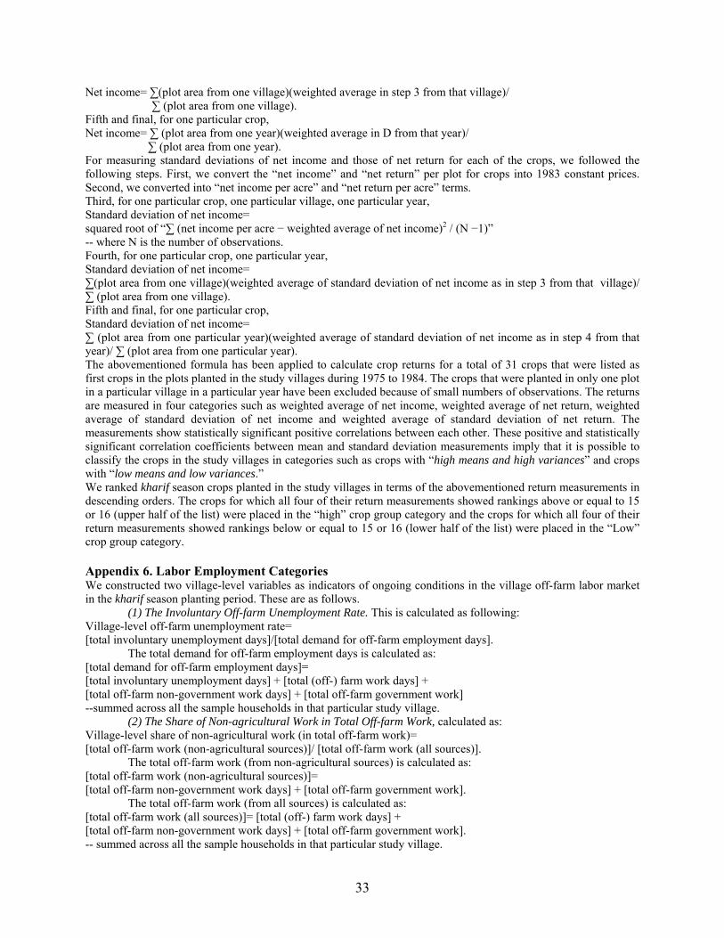
Net income= ∑(plot area from one village)(weighted average in step 3 from that village)/ ∑ (plot area from one village). Fifth and final, for one particular crop, Net income= ∑ (plot area from one year)(weighted average in D from that year)/ ∑ (plot area from one year). For measuring standard deviations of net income and those of net return for each of the crops, we followed the following steps. First, we convert the “net income” and “net return” per plot for crops into 1983 constant prices. Second, we converted into “net income per acre” and “net return per acre” terms. Third, for one particular crop, one particular village, one particular year, Standard deviation of net income= squared root of “∑ (net income per acre − weighted average of net income)2 / (N −1)” -- where N is the number of observations. Fourth, for one particular crop, one particular year, Standard deviation of net income= ∑(plot area from one village)(weighted average of standard deviation of net income as in step 3 from that village)/ ∑ (plot area from one village). Fifth and final, for one particular crop, Standard deviation of net income= ∑ (plot area from one particular year)(weighted average of standard deviation of net income as in step 4 from that year)/ ∑ (plot area from one particular year). The abovementioned formula has been applied to calculate crop returns for a total of 31 crops that were listed as first crops in the plots planted in the study villages during 1975 to 1984. The crops that were planted in only one plot in a particular village in a particular year have been excluded because of small numbers of observations. The returns are measured in four categories such as weighted average of net income, weighted average of net return, weighted average of standard deviation of net income and weighted average of standard deviation of net return. The measurements show statistically significant positive correlations between each other. These positive and statistically significant correlation coefficients between mean and standard deviation measurements imply that it is possible to classify the crops in the study villages in categories such as crops with “high means and high variances” and crops with “low means and low variances.” We ranked kharif season crops planted in the study villages in terms of the abovementioned return measurements in descending orders. The crops for which all four of their return measurements showed rankings above or equal to 15 or 16 (upper half of the list) were placed in the “high” crop group category and the crops for which all four of their return measurements showed rankings below or equal to 15 or 16 (lower half of the list) were placed in the “Low” crop group category. Appendix 6. Labor Employment Categories We constructed two village-level variables as indicators of ongoing conditions in the village off-farm labor market in the kharif season planting period. These are as follows. (1) The Involuntary Off-farm Unemployment Rate. This is calculated as following: Village-level off-farm unemployment rate= [total involuntary unemployment days]/[total demand for off-farm employment days]. The total demand for off-farm employment days is calculated as: [total demand for off-farm employment days]= [total involuntary unemployment days] + [total (off-) farm work days] + [total off-farm non-government work days] + [total off-farm government work] --summed across all the sample households in that particular study village.

(2) The Share of Non-agricultural Work in Total Off-farm Work, calculated as: Village-level share of non-agricultural work (in total off-farm work)= [total off-farm work (non-agricultural sources)]/ [total off-farm work (all sources)]. The total off-farm work (from non-agricultural sources) is calculated as: [total off-farm work (non-agricultural sources)]= [total off-farm non-government work days] + [total off-farm government work]. The total off-farm work (from all sources) is calculated as: [total off-farm work (all sources)]= [total (off-) farm work days] + [total off-farm non-government work days] + [total off-farm government work]. -- summed across all the sample households in that particular study village.

33

References Antle, J. M., (1983), “Incorporating Risk in Production Analysis,” American Journal of Agricultural

Economics, 65(5), 1099-1106 Arrow, K. J., (1964), “The Role of Securities in the Optimal Allocation of Risk-Bearing,” Review of

Economic Studies, 31(2), 91-96. Originally published as “Le Role Des Valeurs Boursieres Pours la Repartition la Meilleure des Risqes” in Econometrie. Centre National de la Recherche Scientifique, Paris, 1953

Bardhan, P. and C. Udry, (1999), Development Microeconomics, Oxford and New York: Oxford University Press

Debreu, G., (1959), Theory of Value: An Axiomatic Analysis of Economic Equilibrium, New York: John Wiley & Sons, Ltd.

Feder, G., (1977), “The Impact of Uncertainty in a Class of Objective Functions”, Journal of Economic Theory, 16(2), 503-512

Honore, B. E., (1992), “Trimmed Lad and Least Squares Estimation of Truncated and Censored Regression Models with Fixed Effects”, Econometrica, 60(3), 533-565

Intriligator, M. D., (1971), Mathematical Optimization and Economic Theory, New Jersey: Prentice-Hall, Englewood Cliffs

Just, R. E. and R. D. Pope, (1978), “Stochastic Specification of Production Functions and Economic Implications,” Journal of Econometrics, 7(1), 67-86

Kanwar, S., (1999), “Does Risk Matter? The Case of Wage-labour Allocation by Owner-Cultivators,” Applied Economics, 31(1), 307-317

Kochar, A., (1999), “Smoothing Consumption by Smoothing Income: Hours-of-Work Responses to Idiosyncratic Agricultural Shocks in Rural India,” Review of Economics and Statistics, 81(1), 50-61

Kurosaki, T., (1998), Risk and Household Behavior in Pakistan's Agriculture, I.D.E. Occasional Papers Series, 34, Japan: Institute of Developing Economies

Lamb, R. L., (2003), “Fertilizer Use, Risk and Off-farm Labor Markets in the Semi-Arid Tropics of India,” American Journal of Agricultural Economics, 85(2), 359-371

Pope, R. D. and R. Kramer, (1979), “Production Uncertainty and Factor Demands for the Competitive Firm,” Southern Economic Journal, 46(2), 489-501

Roe, T. and T. Graham-Tomasi, (1986), “Yield Risk in a Dynamic Model of the Agricultural Household,” in Singh, I., L. Squire and J. Strauss (eds.), Agricultural Household Models: Extensions, Applications and Policy, Baltimore: The Johns Hopkins University Press

Rose, E., (1993), Ex ante and Ex post Labor Supply Response to Risk in a Low-Income Area, Ph.D. Dissertation, University of Pennsylvania, Philadelphia.

Rose, E., (2001), “Ex ante and Ex post Labor Supply Response to Risk in a Low-income Area,” Journal of Development Economics, 64(2), 371-388

Rosenzweig, M. R. and H. P. Binswanger, (1993), “Wealth, Weather Risk and the Composition and Profitability of Agricultural Investments,” Economic Journal, 103(416), 56-78

Singh, I., L. Squire and J. Strauss, (1986), “Methodological Issues,” in Singh, I., L. Squire and J. Strauss (eds.), Agricultural Household Models: Extensions, Applications and Policy, Baltimore: The Johns Hopkins University Press

Singh, R.P., H. P. Binswanger and N.S. Jodha, (1985), Manual of Instructions for Economic Investigators in ICRISAT’s Village Level Studies (Revised), Mimeograph, India: International Crop Research Institute for the Semi-Arid Tropics

Walker, T. S. and J. G. Ryan, (1990), Village and Household Economies in India’s Semi-Arid Tropics, Baltimore: The Johns Hopkins University Press

Wooldridge, J. M., (2002), Econometric Analysis of Cross Section and Panel Data, Cambridge and London: The MIT Press

34