Multivariate peaks over thresholds models - Springer · Multivariate peaks over thresholds models...

Extremes (2018) 21:115–145DOI 10.1007/s10687-017-0294-4

Multivariate peaks over thresholds models

Holger Rootzen1 ·Johan Segers2 ·Jennifer L. Wadsworth3

Received: 18 October 2016 / Revised: 20 April 2017 / Accepted: 21 April 2017 /Published online: 23 June 2017© The Author(s) 2017. This article is an open access publication

Abstract Multivariate peaks over thresholds modelling based on generalized Paretodistributions has up to now only been used in few and mostly two-dimensional sit-uations. This paper contributes theoretical understanding, models which can respectphysical constraints, inference tools, and simulation methods to support routine use,with an aim at higher dimensions. We derive a general point process model forextreme episodes in data, and show how conditioning the distribution of extremeepisodes on threshold exceedance gives four basic representations of the familyof generalized Pareto distributions. The first representation is constructed on thereal scale of the observations. The second one starts with a model on a standardexponential scale which is then transformed to the real scale. The third and fourthrepresentations are reformulations of a spectral representation proposed in Ferreiraand de Haan (Bernoulli 20(4), 1717–1737, 2014). Numerically tractable forms ofdensities and censored densities are found and give tools for flexible parametric like-lihood inference. New simulation algorithms, explicit formulas for probabilities andconditional probabilities, and conditions which make the conditional distribution ofweighted component sums generalized Pareto are derived.

� Holger [email protected]

Johan [email protected]

Jennifer L. [email protected]

1 Chalmers and Gothenburg University, Goteborg, Sweden

2 Universite catholique de Louvain, Louvain-la-Neuve, Belgium

3 Lancaster University, Lancaster, UK

http://crossmark.crossref.org/dialog/?doi=10.1007/s10687-017-0294-4&domain=pdf

http://orcid.org/0000-0001-8869-7989

http://orcid.org/0000-0002-0444-689X

http://orcid.org/0000-0003-2059-1234

mailto:[email protected]



116 H. Rootzen et al.

Keywords Extreme values · Multivariate generalized Pareto distribution · Peaksover threshold likelihoods · Simulation of extremes

AMS 2000 Subject Classifications 62G32 · 60G70 · 62E10

1 Introduction

Peaks over thresholds (PoT) modelling was introduced in the hydrological litera-ture (NERC 1975). The philosophy is simple: extreme events, perhaps extreme waterlevels, are often quite different from ordinary everyday behaviour, and ordinarybehaviour then has little to say about extremes, so that only other extreme eventsgive useful information about future extreme events. To make this idea operational,one defines an extreme event as a value, say a water level, which exceeds some highthreshold, and only uses the sizes of the excesses over this threshold, the “peaks overthe threshold”, for statistical inference. This idea was given a theoretical foundationby combining it with asymptotic arguments motivating that the natural model is thatexceedances occur according to a Poisson process and that excess sizes follow a gen-eralized Pareto (GP) distribution (Balkema and de Haan 1974; Pickands 1975; Smith1984; Davison and Smith 1990).

Since then, numerous papers have used one-dimensional PoT models (thoughoften not under this name), in areas ranging from earth and atmosphere science tofinance, see e.g. Kysely et al. (2010), Katz et al. (2002), and McNeil et al. (2015).The method has also been presented in a number of books, see e.g. Coles (2001),Beirlant et al. (2004), and Dey and Yan (2015).

However, often it is not just one extreme event which is important, but an entireextreme episode. In the 2005 flooding of New Orleans caused by windstorm Katrina,more than 50 levees were breached. However, many others held, and damage wasdetermined by which levees held and which were flooded (Andersen et al. 2007).Extreme rain can lead to devastating landslides, and can be caused by one day withvery extreme rainfall, or by two or more consecutive days with smaller, but stillextreme rain amounts (Guzzetti et al. 2007). The 2003 heat-wave in central Europe isestimated to have killed between 25 000 and 70 000 people. Many deaths, however,were not caused by one extremely hot day, but rather by a long sequence of high min-imum nightly temperatures which led to increasing fatigue and eventually to death(Grynszpan 2003). These and very many other important societal problems under-line the importance of statistical methods which can handle multivariate extremeepisodes.

Using the same philosophy as for extreme events in one dimension, PoT modellingof extreme episodes proceeds by choosing a high threshold for each component ofthe episode, and then to consider an episode as extreme if at least one componentexceeds its threshold. One then only models the difference between the values ofthe components and their respective thresholds. However, in the multivariate case allthe componentwise differences in an extreme episode are modelled, both the over-shoots and the undershoots. For instance, in a rainfall episode affecting a numberof catchments, both the amount of rain in the catchments where rainfall exceeds the

Multivariate peaks over thresholds models 117

threshold and in catchments where the threshold is not exceeded are important. Addi-tionally, the inclusion of undershoots increases the amount of information that canbe used for inference. Just as in one dimension, the natural model is that extremeepisodes occur according to a Poisson process and that overshoots and undershoots(or undershoots larger than a censoring threshold) jointly follow a multivariate GPdistribution.

The aim of this paper is to contribute probabilistic understanding, physically moti-vated models, likelihood tools, and simulation methods, all of which are needed formultivariate PoT modelling of extreme episodes via multivariate GP distributions.Specifically, the key contributions are: new representations of GP distributions con-ducive to model construction; density formulas for each of these representations;new properties of multivariate GP distributions; and simulation tools. Many of theseresults are oriented towards enabling improved statistical modelling, but here werestrict ourselves to a probabilistic study. A companion paper (Kiriliouk et al. 2016)addresses practical modelling aspects.

We begin by deriving the basic properties of the class of multivariate GPdistributions. We then pursue the following program:

(i) to exhibit the possible point process limits of extreme episodes in data;(ii) to show how conditioning on threshold exceedances transforms the distribution

of the extreme episodes to GP distributions, and to use this to find physicallymotivated representations of the multivariate GP distributions; and

(iii) to derive likelihoods and censored likelihoods for the representations in (ii).

In part (ii) of the program, we develop four representations. The first one is inthe same units as the observations, i.e., on the real scale, and in the second one themodel is built on a standard exponential scale and then transformed to the real obser-vation scale. The third is a spectral representation proposed in Ferreira and de Haan(2014), and the fourth one a simple reformulation of this representation aimed at aid-ing model construction. A useful, and to us surprising, discovery is that it is possibleto derive the density also for the fourth representation, and that this density in factis simpler than the densities for the other two first representations. The importanceof (iii) is that likelihood inference makes it possible to incorporate covariates, e.g.temporal or spatial trends, in a flexible and practical way.

The insights and results obtained in carrying out this program, we believe, willlead to new models, new computational techniques, and new ways to make the neces-sary compromises between modelling realism and computational tractability whichtogether will make possible routine use, also in dimensions higher than two. Thelimiting factor is the number of parameters rather than the number of variables. Themodels mentioned in Example 3 may be a case in point. The formulas for probabil-ities, conditional probabilities and conditional densities given in Sections 5 and 6,together with the discovery that weighted sums of components of GP distributionsconditioned to be positive also have a GP distribution, add to the usefulness of themethods. Simulation of GP distributions is needed for several reasons, includingcomputation of the probabilities of complex dangerous events and goodness of fitchecking. The final contribution of this paper is a number of simulation algorithmsfor multivariate GP distributions.


The multivariate GP distributions were introduced in Tajvidi (1996), Beirlant et al.(2004, Chapter 8), and Rootzen and Tajvidi (2006); see also Falk et al. (2010, Chap-ter 5). A closely related approximation was used in Smith et al. (1997). The literatureon applications of multivariate PoT modelling is rather sparse (Brodin and Rootzen2009; Michel 2009; Aulbach et al. 2012). Some earlier papers use point process mod-els which are closely related to the PoT/GP approach (Coles and Tawn 1991; Joeet al. 1992). Other papers consider nonparametric or semiparametric rank-based PoTmethods focusing on the dependence structure but largely ignoring modelling themargins (de Haan et al. 2008; Einmahl et al. 2012; Einmahl et al. 2016). However, theGP approach has the advantages that it provides complete models for the thresholdexcesses, that it can use well-established model checking tools, and that, comparedto the point process approach, it leads to more natural parametrizations of trends inthe Poisson process which governs the occurrence of extreme episodes.

There is an important literature on modelling componentwise, perhaps yearly,maxima with multivariate generalized extreme value (GEV) distributions: for asurvey in the spatial context see Davison et al. (2012). However, componentwisemaximamay occur at different times for different components, and in many situationsthe focus is on the PoT structure: extremes which occur simultaneously. Addition-ally, likelihood inference for GEV distributions is complicated by a lack of tractableanalytic expressions for high-dimensional densities, so that inference often is mucheasier, and perhaps more efficient, in GP models; see Huser et al. (2015) for a sur-vey and an extensive comparison. The most important special case of GP models arethose for which all variables can be simultaneously extreme, and there is no massplaced on hyperplanes (see Section 2 for details of the support); this is a typical mod-elling assumption. Further comment on the situation of asymptotic independence,where this does not hold, is made in Section 8, as well as in Kiriliouk et al. (2016).

Section 2 derives and exemplifies the basic properties of the GP cumulative distri-bution functions (cdf-s). In Section 3 we develop a point process model of extremeepisodes, and Section 4 shows how conditioning on exceeding high thresholds leadsto three basic representations of the GP distributions. Section 5 exhibits the fourthrepresentation and derives densities and censored likelihoods, while Section 6 givesformulas for probabilities and conditional probabilities in GP distributions. Finally,Section 7 contributes simulation algorithms for multivariate GP distributions andSection 8 discusses parametrization issues and gives a concluding overview.

2 Multivariate generalized Pareto distributions

This section first briefly recalls and adapts existing theory for multivariate GEVdistributions, and then derives a number of the basic properties of GP distributions.

Throughout we use notation as follows. The maximum and minimum operatorsare denoted by the symbols ∨ and ∧, respectively. Bold symbols denote d-variatevectors. For instance, α = (α1, . . . , αd) and 0 = (0, . . . , 0) ∈ R

d . Operations andrelations involving such vectors are meant componentwise, with shorter vectors beingrecycled if necessary. For instance ax + b = (a1x1 + b1, . . . , adxd + bd), x ≤ y

if xj ≤ yj for j = 1, . . . , d , and tγ = (tγ1 , . . . , tγd ). If F is a cdf then we write


F = 1 − F for its tail function, and also write F for the probability distribution

determined by the cdf. That X ∼ F means that X has distribution F , andd−→ denotes

convergence in distribution. The symbol 1 is the indicator function: 1A equals 1 onthe set A and 0 otherwise.

For fixed γ ∈ R, the functions x �→ (xγ −1)/γ (for x > 0) and x �→ (1+γ x)1/γ

are to be interpreted as their limits log(x) and exp(x), respectively, if γ = 0. Thisconvention also applies componentwise to expressions of the form (xγ − 1)/γ and(1 + γ x)1/γ .

Below we repeatedly use that if X is a d-dimensional vector with P(X � u) > 0and s > 0 then

P[s(X−u) ≤ x | X−u � 0] = P[X ≤ x/s + u] − P[X ≤ (x ∧ 0)/s + u]P[X � u] . (2.1)

2.1 Background: multivariate generalized extreme value distributions

Throughout, G denotes a d-variate GEV distribution, so that in particular G hasnon-degenerate margins. The class of GEV distributions has the following equiv-alent characterizations, see e.g. Beirlant et al. (2004): (M1) It is the class of limitdistributions of location-scale normalized maxima, i.e., the distributions which arelimits

P[a−1n (∨d

i=1 Xi − bn) ≤ x] d−→ G(x), as n → ∞, (2.2)

of normalized maxima of independent and identically distributed (i.i.d.) vectorsX1, X2, . . . ∼ F , for an > 0 and bn; and (M2) It is the class of max-stable distribu-tions, i.e., distributions such that taking maxima of i.i.d. vectors from the distributiononly leads to a location-scale change of the distribution. By (M1) the class of GEVdistributions is closed under location and scale changes.

The marginal distribution functions, G1, . . . , Gd , of G may be written as

Gj(x) = exp

{

−(1 + γj

x−μj

αj

)−1/γj}

, (2.3)

for x ∈ R such that αj +γj (x−μj ) > 0. We will use this parametrization throughout.The parameter range is (γj , μj , αj ) ∈ R × R × (0, ∞). Define

σ = α − γμ,

so that σj = αj − γjμj , j ∈ {1, . . . , d}. Then Gj is supported by the interval

Ij =⎧⎨

⎩

(−σj/γj , ∞) if γj > 0,(−∞, ∞) if γj = 0,(−∞, −σj/γj ) if γj < 0,

(2.4)

while G is supported by a (subset of) the rectangle I1×· · ·× Id . The lower and upperendpoints of Gj are denoted by ηj ∈ R ∪ {−∞} and ωj ∈ R ∪ {+∞}, respectively.One may alternatively write the condition x ∈ I1 × · · · × Id as γ x + σ > 0.

Below we assume that 0 < G(0) < 1. This inequality is equivalent to Gj(0) > 0for all j ∈ {1, . . . , d} andGj(0) < 1 for some j ∈ {1, . . . , d}. The equivalence followsfrom positive quadrant dependence,G(0) ≥∏d

j=1 Gj(0) (Marshall and Olkin 1983).


PoT models are determined by the difference between the thresholds and the locationparameters of the observations, and not by their individual values. Hence, it doesnot entail any loss of generality to shift the location parameters {μi} to make theassumption 0 < G(0) < 1 hold.

We will often use the stronger condition that σ > 0, i.e., that σj > 0 for allj ∈ {1, . . . , d}. By Eq. 2.4, this is equivalent to assuming that 0 is in the interior ofthe support of every one of the d margins G1, . . . , Gd , i.e., that ηj < 0 < ωj andthus 0 < Gj(0) < 1 for all j ∈ {1, . . . , d}. This is an additional restriction only forγj < 0: if γj = 0, then σj = αj > 0, while if γj > 0 then G(0) > 0 implies ηj < 0and thus σj = −γjηj > 0.

An easy argument shows that G is max-stable if and only if for each t > 0 thereexist scale and location vectors at ∈ (0, ∞)d and bt ∈ R

d such that G(atx + bt )t ≡

G(x) (Resnick 1987, Equation (5.17)). It follows from Eq. 2.3 that these parametersare given by

at = tγ , bt = σ (tγ − 1)/γ . (2.5)

To a GEV distribution G we can associate a Borel measure ν on∏d

j=1[−ηj , ∞) \{η} by the formula ν({y; y ≤ x}) = − logG(x) for x ∈ [−∞, ∞)d , with the con-vention that − log(0) = ∞ (Resnick 1987, Proposition 5.8). The measure ν is calledintensity measure because, by (M1), the limit of the expected number of location-scale normalized points, say a−1

n (Xi − bn), i ∈ {1, . . . , n}, in a Borel set A whichis bounded away from η and such that ν(∂A) = 0, is equal to ν(A). The inten-sity measure ν determines the limit distribution of the sequence of point processes∑n

i=1 δa−1

n (Xi−bn), see Section 3.

2.2 Generalized Pareto distributions

Let G be a GEV distribution with 0 < G(0) < 1 and let ν be the correspondingintensity measure. Then 0 < ν({y; y ≤ 0}) < ∞, so that we can define a probabilitymeasure supported by the set {y; y ≤ 0} by restricting the intensity measure ν tothat set and normalizing it. The result is the generalized Pareto (GP) distributionassociated to G. Its cdf H may be expressed as

H(x) =

⎧⎪⎨

⎪⎩

1

logG(0)log

(G(x ∧ 0)

G(x)

)

if x > η,

0 if xj < ηj for some j = 1, . . . , d ,(2.6)

see Beirlant et al. (2004, Chapter 8) and Rootzen and Tajvidi (2006). If a GEV cdf G

and a GP cdf H satisfy (2.6), then we say that they are associated and write H ↔ G.For completeness, we prove (2.6) in the Appendix. For points x ∈ [−∞, ∞)d withx ≥ η and xj = ηj for some j , the value of H(x) is determined by right-handcontinuity. Below it is shown that η is determined by the values of H(x) for x ≥ 0.

The probability that the j -th component, j ∈ {1, . . . , d}, exceeds zero is equalto 1 − Hj(0) = logGj(0)/ logG(0), which is positive if and only if Gj(0) < 1,that is, when σj = αj − γjμj > 0. Since G(0) < 1 implies that Gj(0) < 1 forsome but not necessarily all j , the GP family includes distributions for which one (orseveral) of the components never exceed their threshold, so that the support of that


component lies in [−∞, 0]. This could be useful in some modelling situations, butstill, the situation of main interest is when all components have a positive probabilityof being an exceedance, or equivalently when Hj(0) < 1 for all j ∈ {1, . . . , d}, or,again equivalently, when σ > 0.

Similarly to the characterizations (M1) and (M2) of the GEV distributions, theclass of GP distributions H such that Hj(0) < 1 for all j ∈ {1, . . . , d} has thefollowing characterizations (Rootzen and Tajvidi 2006).1 The functions σ t , ut inthe characterizations are assumed to be continuous, and additionally ut is assumedincreasing.

(T1) The GP distributions are limits of distributions of threshold excesses: Let X ∼F . If there exist scaling and threshold functions st ∈ (0, ∞)d and ut ∈ R

d

with F(ut ) < 1 and F(ut ) → 1 as t → ∞, such that

P[s−1t (X − ut ) ∨ 0 ≤ · | X � ut ] d−→ H+, as t → ∞,

for some cdfH+ with nondegenerate margins, then the functionH+(x); x > 0can be uniquely extended to a GP cdf H(x); x ∈ R

d , and

P[s−1t (X − ut ) ∨ η ≤ · | X � ut ] d−→ H, as t → ∞. (2.7)

(T2) The GP distributions are threshold-stable: Let X ∼ H where H has non-degenerate margins on R+. If there exist scaling and threshold functionsst ∈ (0, ∞)d and ut ∈ R

d , with u1 = 0 and H(ut ) → 1 as t → ∞, such that

P[s−1t (X − ut ) ≤ x | X � ut ] = H(x) (2.8)

for x ≥ 0 then there is an uniquely determined GP cdf H such that H (x) =H(x) for x > η. Conversely, all GP distributions H for which Hj(0) < 1 forall j ∈ {1, . . . , d} satisfy (2.8) for all x ∈ R

d .

We use the term “threshold-stable” for property (T2) in analogy with the terms“sum-stable” and “max-stable”. A distribution is sum- or max-stable if the sum ormaximum, respectively, of independent variables with this distribution has the samedistribution, up to a location-scale change. Analogously, a distribution is threshold-stable if conditioning on the exceedance of suitable higher thresholds leads todistributions which, up to scale changes, are the same as the original distribution.This property is illustrated in Fig. 1, with ut and st as given below in Theorem 1(viii).

If (T1) holds we say that F belongs to the (threshold) domain of attraction ofH . In contrast to the limit in (M1), different threshold functions can lead to limitswhich are not location-scale transformations of one another. A cdf F is in a domainof attraction for maxima if and only if it is in a threshold domain of attraction.

The GP distribution H is supported by the set

[η, ω] \ [η, 0] = {x ∈ Rd : ηj ≤ xj ≤ ωj for all j , and xj > 0 for some j}.

1In the article, the truncation factor “ ∨η” is missing in Theorem 2.2 and Theorem 2.3 (ii). A correctionnote is forthcoming.


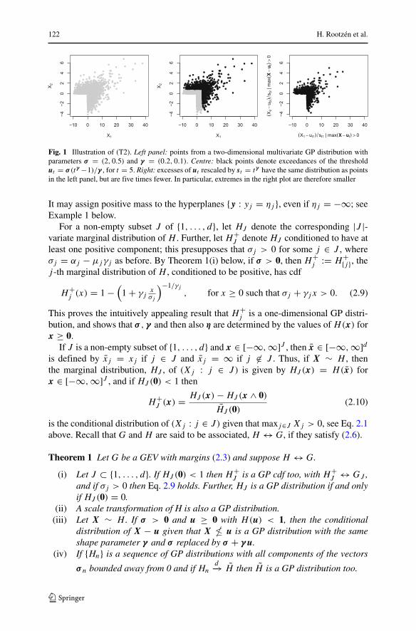
Fig. 1 Illustration of (T2). Left panel: points from a two-dimensional multivariate GP distribution withparameters σ = (2, 0.5) and γ = (0.2, 0.1). Centre: black points denote exceedances of the thresholdut = σ (tγ −1)/γ , for t = 5. Right: excesses of ut rescaled by st = tγ have the same distribution as pointsin the left panel, but are five times fewer. In particular, extremes in the right plot are therefore smaller

It may assign positive mass to the hyperplanes {y : yj = ηj }, even if ηj = −∞; seeExample 1 below.

For a non-empty subset J of {1, . . . , d}, let HJ denote the corresponding |J |-variate marginal distribution of H . Further, let H+

J denote HJ conditioned to have atleast one positive component; this presupposes that σj > 0 for some j ∈ J , whereσj = αj − μjγj as before. By Theorem 1(i) below, if σ > 0, then H+

j := H+{j}, the

j -th marginal distribution of H , conditioned to be positive, has cdf

H+j (x) = 1 −

(1 + γj

xσj

)−1/γj

, for x ≥ 0 such that σj + γjx > 0. (2.9)

This proves the intuitively appealing result that H+j is a one-dimensional GP distri-

bution, and shows that σ , γ and then also η are determined by the values of H(x) forx ≥ 0.

If J is a non-empty subset of {1, . . . , d} and x ∈ [−∞, ∞]J , then x ∈ [−∞, ∞]dis defined by xj = xj if j ∈ J and xj = ∞ if j ∈ J . Thus, if X ∼ H , thenthe marginal distribution, HJ , of (Xj : j ∈ J ) is given by HJ (x) = H(x) forx ∈ [−∞, ∞]J , and if HJ (0) < 1 then

H+J (x) = HJ (x) − HJ (x ∧ 0)

HJ (0)(2.10)

is the conditional distribution of (Xj : j ∈ J ) given that maxj∈J Xj > 0, see Eq. 2.1above. Recall that G and H are said to be associated, H ↔ G, if they satisfy (2.6).

Theorem 1 Let G be a GEV with margins (2.3) and suppose H ↔ G.

(i) Let J ⊂ {1, . . . , d}. If HJ (0) < 1 then H+J is a GP cdf too, with H+

J ↔ GJ ,and if σj > 0 then Eq. 2.9 holds. Further, HJ is a GP distribution if and onlyif HJ (0) = 0.

(ii) A scale transformation of H is also a GP distribution.(iii) Let X ∼ H . If σ > 0 and u ≥ 0 with H(u) < 1, then the conditional

distribution of X − u given that X � u is a GP distribution with the sameshape parameter γ and σ replaced by σ + γu.

(iv) If {Hn} is a sequence of GP distributions with all components of the vectors

σ n bounded away from 0 and if Hnd−→ H then H is a GP distribution too.


(v) A finite or infinite mixture of GP distributions with the same σ and γ is a GPdistribution.

(vi) We have H ↔ Gt for all t > 0. Conversely, if H ↔ G∗ for some G∗ and ifσ > 0 then G∗ = Gt1 for some t1 > 0.

(vii) If G(0) = e−v then G(x) = exp{−vH (x)}, x ≥ 0, and if σ > 0 thisdetermines G.

(viii) If σ > 0, the scaling and threshold functions in the (T2) characterization ofGP distributions may be taken as st = tγ and ut = σ (tγ − 1)/γ , for t ≥ 1.

(ix) The parameters γ and σ are identifiable from H .

In words, Theorem 1(i) says that conditional margins of GP distributions are GP,but that marginal distributions of GP distribution are typically not GP. For instance,if H is a two-dimensional GP cdf, then H+

1 is a one-dimensional GP cdf (given by(2.9)), but typically H1 is not. Intuitively, the reason is that the conditioning eventimplicit in H1(x) also includes the possibility that it is the second component, ratherthan the first one, that exceeds its threshold. Theorem 1 (ii)−(v) also establish closureproperties of the class of GP distributions. By (vi) and (vii) a GEV distribution speci-fies the associated GP distribution and conversely a GP distribution specifies a curveof associated GEV distributions in the space of distribution functions. Regarding(vii), note that a GEV distribution G such that 0 < Gj(0) < 1 for all j is determinedby its values for x ≥ 0 (proof in the Appendix). Finally, (viii) identifies the affinetransformations which leave H unchanged, and (ix) establishes identifiability of themarginal parameters.

Proof (i) Let 0 denote x for the special case when x = 0 ∈ (−∞, ∞)J and letGJ (x) = G(x) be the marginal distribution of G. Clearly x∧0 = (x ∧ 0)∧0and hence, for x > η,

HJ (x) − HJ (x ∧ 0)

= 1

logG(0)log

(G(x ∧ 0)

G(x)

)

− 1

logG(0)log

(G((x ∧ 0) ∧ 0)

G(x ∧ 0)

)

= 1

logG(0)log

(GJ (x ∧ 0)

GJ (x)

)

and

HJ (0) = 1 − 1

logG(0)log

(G(0 ∧ 0)

G(0)

)

= logGJ (0)logG(0)

,

so that

H+J (x) = 1

logGJ (0)log

(GJ (x ∧ 0)

GJ (x)

)

.

Inserting (2.3) into the equation above for J = {j} together with straight-forward calculation proves (2.9), and hence completes the proof of the firstassertion.

If HJ (0) = 0, then HJ = H+J and it follows from the first assertion that

HJ is a GP distribution function. Further, GP distributions are supported by


{y; y � 0} and hence if HJ (0) > 0 then HJ is not a GP cdf. This proves thesecond assertion.

(ii) If G is a GEV cdf then, for s > 0, the map x �→ G(x/s) is a GEV cdf too,and the result then follows from

H(x/s)= 1

logG(0)log

(G((x/s) ∧ 0)logG(x/s)

)

= 1

logG(0/s)log

(G((x ∧ 0)/s)

G(x/s)

)

.

(iii) Proceeding as in the proof of (i), but in the first step instead using that (x +u) ∧ 0 = (x ∧ 0 + u) ∧ 0, shows that the conditional distribution of X − u

given that X � u is

H(x + u) − H(x ∧ 0 + u)

H (u)= 1

logG(u)log

(G(x ∧ 0 + u)

G(x + u)

)

.

The map x �→ G(x) = G(x + u) is also a GEV cdf, but with the vectorσ = α − γμ replaced by σ = α − γ (μ − u) = σ + γu.

(iv) Convergence in distribution in Rd implies convergence of the marginal dis-

tributions, and using standard converging subsequence arguments it followsfrom marginal convergence that there exist σ > 0 and γ such that σ n → σ

and γ n → γ . Define un,t and sn,t from Hn as in Eq. 2.8 (vi). Then, sinceHn is a GP cdf we have, using first (T2) and (viii), and then the continuousmapping theorem, that

Hn(x) = Hn(x/sn,t + un,t ) − Hn((x/sn,t ) ∧ 0 + un,t )

Hn(un,t )

d→ H (x/st + ut ) − H ((x/st ) ∧ 0 + ut )

¯H(ut )

, as n → ∞.

Since Hnd→ H it follows that H satisfies (T2) and hence is a GP cdf.

(v) We only prove that a mixture of two GP cdf-s with the same σ and γ is aGP cdf too, using Theorem 4 below (the proof of that theorem does not usethe result we are proving now). The proof for arbitrary finite mixtures is thesame, and the result for infinite mixtures then follows by taking limits of finitemixtures and using (iv). Let H1 and H2 be GP cdf-s with the same marginalparameters σ , γ and let p ∈ (0, 1). By Theorem 4 and Eq. 4.2 there exists cdf-s Fi = FRi such that Hi(x) = ci

∫∞0 {Fi(t

γ (x + σγ))−Fi(t

γ (x ∧ 0+ σγ))} dt

with ci = 1/∫∞0 Fi(t

γ σγ) dt , and with the convention that if γi = 0 then

tγi (xi + σi

γi) is interpreted to mean xi +σi log t . Writing F = pc1

pc1+(1−p)c2F1+

(1−p)c2pc1+(1−p)c2

F2 it follows that

H (x) := pH1(x) + (1 − p)H2(x)

= [pc1 + (1 − p)c2]∫ ∞

0

{F(tγ (x+ σ

γ))−F

(tγ (x ∧ 0 + σ

γ))}

dt.

Straightforward calculation shows that pc1 + (1 − p)c2 = 1/∫∞0 F (tγ σ

γ) dt

so that H (x) satisfies Eq. 4.2 and hence is a GP cdf.


(vi) The first assertion follows from Eq. 2.6. Choose t1 so that − logG(0)t1 =− logG∗(0). Then H ↔ G and H ↔ G∗ imply together that

G(x ∧ 0)t1

G(x)t1= G∗(x ∧ 0)

G∗(x),

and in particular, that G(x)t1 = G∗(x) for x ≥ 0. Since a GEV cdf withσ > 0 is determined by its values for x ≥ 0, see the Appendix, this completesthe proof.

(vii) The first part follows from Eq. 2.6, and that this determines G again followsfrom the appendix.

(viii) By the proofs of (iii) and (vi) the conditional distribution of s−1t (X − ut )

given that X � ut is associated with G(stx + ut ) = G(x)1/t , and the resultfollows from (vii).

(ix) For t > 0, let (γj (t), μj (t), αj (t)) ∈ R×R× (0, ∞) be the parameter vectorof Gt

j , and let σj (t) = αj (t) − γj (t) μj (t). By assertion (vi), the GPD H

determines the curve of GEV-s Gt for t > 0. It suffices to show that γj (t)

and σj (t) do not depend on t . But this follows by straightforward calculationsfrom the max-stability property G(x)t = G(a−1

t (x − bt )) with at and bt asin Eq. 2.5.

Example 1 below exhibits two-dimensional GP distributions with positive masson certain lines, and the first part of Example 2 provides a cdf where the secondassertion in (i) of Theorem 1 comes into play. In contrast to scale transformations,it seems likely that if σ > 0 then a non-trivial location transformation of a GP cdfnever is a GP cdf. The second part of Example 2 shows one of the exceptional caseswhere the support of one of the components is contained in (−∞, 0) and where alocation transformation of a GP distribution does give another GP distribution.

Example 1 This example rectifies the one on pages 1726–1727 in Ferreira and deHaan (2014). Let G(x, y) = exp{−1/(x+1)−1/(y+1)} for (x, y) ∈ (−1, ∞)2, thedistribution of two independent unit Frechet random variables with lower endpointsα1 = α2 = −1. The corresponding multivariate generalized Pareto distribution isgiven by

H(x, y) =

⎧⎪⎪⎪⎪⎪⎨

⎪⎪⎪⎪⎪⎩

12

(1 − 1

x+1 + 1 − 1y+1

)if (x, y) ∈ [0, ∞)2,

12

(1 − 1

x+1

)if (x, y) ∈ [0, ∞) × [−1, 0],

12

(1 − 1

y+1

)if (x, y) ∈ [−1, 0] × [0, ∞),

0 otherwise.

(2.11)

We conclude that H is the distribution function of the random vector (X, Y ) given by

(X, Y ) ={

(−1, T ) with probability 1/2,(T , −1) with probability 1/2,


where T is generalized Pareto, P(T ≤ t) = 1 − 1/(t + 1) for t ≥ 0. Hence H issupported by the union of the two lines {−1}× (0, ∞) and (0, ∞)×{−1}, see Fig. 2,left panel.

If we modify the example by choosing Gumbel rather than Frechet margins, sothat G(x, y) = exp(−e−x − e−y) for (x, y) ∈ R

2, then the GP cdf H is the cdf ofthe vector

(X, Y ) ={

(−∞, T ) with probability 1/2,(T , −∞) with probability 1/2,

where T is a unit exponential random variable, P(T ≤ t) = 1 − e−t for t ∈ [0, ∞).The support of H is the union of two lines {−∞} × (0, ∞) and (0, ∞) × {−∞}through −∞.

Example 2 Let G(x, y) = exp[−1/{(x ∧ y)+ 1}] for (x, y) ≥ −1, the cdf of (Z, Z)

for Z unit Frechet with lower endpoint −1. The corresponding GP cdf is

H(x, y) ={1 − 1

(x∧y)+1 if (x, y) ∈ [0, ∞)2,

0 otherwise.(2.12)

We identify H as the distribution of the random pair (T , T ), where P(T ≤ t) =1 − 1/(t + 1) for t ∈ [0, ∞). The support of H is the diagonal {(t, t) : 0 < t < ∞},see Fig. 2, middle panel. It follows that, e.g., H1(0) = 0 and hence in this exampleH1 = H+

1 .As a variation of the example let G(x, y) = exp[−e−x∧(y+μ)] be the cdf of

(Z, Z − μ), with Z standard Gumbel and μ > 0. The corresponding GP cdf is

H(x, y) = e−(x∧0)∧(y∧0+μ) − e−x∧(y+μ) = e−(x∧0)∧(y+μ) − e−x∧(y+μ), (2.13)

and H is the cdf of (T , T − μ) with T standard exponential. Now, for −μ < ν thelocation transformed cdf H(x, y + ν) equals e−(x∧0)∧(y+ν+μ) − e−x∧(y+ν+μ), whichis the same as in Eq. 2.13, but with μ replaced by ν +μ > 0. Hence also H(x, y +ν)

is a GP cdf. The support of H is shown in the right-hand panel of Fig. 2.

Fig. 2 Supports (solid lines) of the GP distributions H in Eqs. 2.11 (left), 2.12 (middle) and 2.13 (right)


3 Point processes of extreme episodes

The first step in our program for PoT inference is to specify a point process modelfor extreme episodes. This model exhibits extreme episodes as a product processobtained by multiplying a random vector, the “shape” vector, with a random quan-tity, the “intensity” of the episode. (For γ = 0, the model instead is a sum.) Thisis parallel to models commonly used for max-stable processes, see e.g. Schlather(2002). In Section 4 below we obtain basic and physically interpretable representa-tions of the GP distributions by conditioning the product process of extreme episodeson threshold exceedance.

In this and subsequent sections we assume that σ > 0. Let X1, X2, . . . be i.i.d.random vectors with cdf F and marginal cdf-s F1, . . . , Fd , and let an, bn be as inEq. 2.2. Further, let η be the vector of lower endpoints of the limiting GEV distri-bution, see Eq. 2.4 and the sentences right below it. We consider weak limits of thepoint processes

Nn =n∑

i=1

δa−1

n (Xi−bn),

where δx denotes a point mass at x. Define Ij = [−σj/γj , ∞) or [−∞, ∞) or[−∞, −σj/γj ) according to whether γj > 0 or γj = 0 or γj < 0, and set

Sγ = I1 × · · · × Id and Sγ = Sγ \ {η}.The limit point process is specified as follows: Let 0 < T1 < T2 < . . . be the pointsof a Poisson process on [0, ∞) with unit intensity and let (Ri )i≥1 be independentcopies of a random vector R which satisfies Condition 2 below. Further assume thatthe vectors (Ri )i≥1 are independent of (Ti)i≥1, and define the point process

Pr =∑

i≥1

δ(Ri /Tγi −σ/γ ), (3.1)

where, by convention, Ri,j /T0i − σj/0 is interpreted to mean Ri,j − σj log T . The

condition on R is as follows.

Condition 2 The components of the random vector R satisfy Rj ∈ [0, ∞) if γj > 0,Rj ∈ [−∞, ∞) if γj = 0, and Rj ∈ [−∞, 0) if γj < 0, and furthermore 0 <

E[|Rj |1/γj ] < ∞ if γj = 0 and E[exp(Rj/σj )] < ∞ if γj = 0, for j = 1, . . . , d .

Let FR be the cdf of R. For γj = 0, the moment restriction in Condition 2can be seen to be equivalent to requiring that 0 <

∫∞0 P(Rj > tγj xj ) dt < ∞,

if xj ∈ (0, ∞) and γj > 0 or if xj ∈ (−∞, 0) and γj < 0. For γj = 0, themoment condition is instead equivalent to 0 <

∫∞0 P(Rj > σj log t + xj ) dt < ∞,

for xj ∈ (−∞, ∞). For example, if γj < 0, then∫∞0 P(Rj > tγj xj ) dt =

∫∞0 P(|Rj |1/γj > t) dt |xj |−1/γj = E(|Rj |1/γj ) |xj |−1/γj . Since P(Rj > tγj xj ) ≤

FR(tγ x) ≤∑di=1 P(Ri > tγi xi), it in turn follows that the moment condition implies

that 0 <∫∞0 FR(tγ (x + σ/γ )) dt < ∞, if the components xj of x are as above,

and where we have used the convention that t0(xj + σj/0) should be replaced byσj log t + xj .


Theorem 3 Suppose F satisfies (2.2). Then, for some R which satisfies Condition 2,

Nnd→ Pr on Sγ , as n → ∞. (3.2)

Conversely, for any Pr given by Eq. 3.1 there exist a GEV cdf G and an > 0 and bn,with 0 < Gj(bn,j ) < 1 and Gj(bn,j ) → 1 for j = 1, . . . , d , such that Eq. 3.2 holdsfor F = G.

Proof Let Y ∼ G and define Y ∗ by Y ∗j = (1 + γj

αj(Yj − μj ))

1/γj if γj = 0 and

Y ∗j = exp{(Yj − μj )/αj } if γj = 0, for μ, α, γ given by Eq. 2.3 so that the marginal

cdf-s of Y ∗ are standard Frechet. It follows as in Theorem 5 of Penrose (1992) (seealso (de Haan and Ferreira 2006) and Schlather (2002)) that there exists a randomvector R∗ ∈ [0, ∞)d with E(R∗

j ) < ∞ such that Y ∗ has the same distribution assupi≥1 R∗

i /Ti where the random vectors R∗i are i.i.d. copies of R∗ and independent

of the unit rate Poisson process (Ti)i≥1. Reversing the transformation which led fromY to Y ∗, it follows that Y has the same distribution as supi≥1(

αγ(R∗

i )γ /T

γi − σ

γ).

Setting R = αγ(R∗)γ it follow that Y has the same distribution as supi≥1(Ri/T

γi −

σγ) with the Ri satisfying Condition 2, and where throughout expressions should be

interpreted as specified after Eq. 3.1 for γj = 0.For ν the intensity measure of Pr , we have G(x) = exp{−ν({y : y � x})}. By

standard reasoning, convergence in distribution of a−1n (∨n

i=1 Xi − bn) is equivalentto n P[a−1

n (X1 − bn) � x] → − logG(x) = ν({y : y � x}), which implies thatn P[a−1

n (X1−bn) ∈ · ] converges vaguely to ν( · ) on Sγ . By Theorem 5.3 of Resnick(2007) this proves (3.2).

Conversely, given Pr , define the cdf G by G(x) = P[supi≥1(Ri/Tγi − σ

γ) ≤

x]. Straightforward calculation as in Schlather (2002, Theorem 2) show that G ismax-stable. Hence there exist sequences an and bn with the stated properties suchthat for independent random vectors X1, X2, . . . with common distribution G, thedistribution of a−1

n (∨n

i=1 Xi − bn) is equal to G too. By the first part of the proof,this proves (3.2).

In the proof of Theorem 3 we obtained part of the following result, which werecord here for completeness.

Corollary 1 Suppose R satisfies Condition 2. Then G(x) = P[supi≥1(Ri/Tγi −

σγ) ≤ x] is a GEV cdf and

G(x) = exp

{

−∫ ∞

0FR

(tγ(x + σ

γ

))dt

}

for x ∈ Sγ , (3.3)

and to any GEV cdf there exists an R which satisfies this equation. Here we use theconvention that t0(xj + σj/0) should be replaced by σj log t + xj .

Proof Writing ν for the intensity measure of Pr we have ν({y; y � x}) =∫∞0 FR(tγ (x + σ

γ)) dt . The right-hand side of Eq. 3.3 is therefore equal to the


probability that Pr has no points in the set {y; y � x}. The result now follows fromthe proof of Theorem 3.

4 Representations of multivariate GP distributions

This section contains the second step in the program for PoT inference. We show howconditioning on threshold exceedances in the point process (3.1) gives four widelyuseful representations of the class of multivariate GP distributions. The first represen-tation, (R) is on the real scale and corresponds to the point process Pr in Eq. 3.1 withpoints obtained as products of shape vectors and intensity variables. In the secondrepresentation, (U), the basic model is constructed on a standard scale and then trans-formed to the real scale. The third representation, (S), is equivalent to the spectralrepresentation in Ferreira and de Haan (2014). A fourth representation, (T ), which isa variation of the (S) representation, is introduced in Section 5.

In the literature the standard scale is chosen as one of the following: Pareto scale,γ = 1, uniform scale, γ = −1, or exponential scale, γ = 0. Here we choosethe γ = 0 scale because of the simple additive structure it leads to. For all fourrepresentations, it is straightforward to switch from one scale to another one.

To understand the GP representation (R) we first approximate Pr by a trun-cated point process Pr where {Ti} is replaced by a unit rate Poisson process {Ti}on a bounded interval [0, K]. Recalling the representation of {Ti} as a Poisson dis-tributed number of Unif [0, K] variables, Pr consists of a Poisson number of vectorsR/T γ − σ

γwith T ∼ Unif [0, K]. Thus, for large n, a point a−1

n (X − bn) in Nn has

approximately the same distribution as R/T γ − σγ. Hence, by Eq. 2.1,

P[a−1n (X − bn) ≤ x | X − bn � 0] ≈ P[R/T γ − σ

γ≤ x | R/T γ − σ

γ� 0]

=1K

∫ K

0 {FR(tγ (x + σγ)) − FR(tγ (x ∧ 0 + σ

γ))} dt

1K

∫ K

0 FR(tγ σγ) dt

=∫ K

0 {FR(tγ (x + σγ)) − FR(tγ (x ∧ 0 + σ

γ))} dt

∫ K

0 FR(tγ σγ) dt

. (4.1)

By the assumptions in Condition 2, the limit as K → ∞ of this expression,

HR(x) =∫∞0 {FR(tγ (x + σ

γ)) − FR(tγ (x ∧ 0 + σ

γ))} dt

∫∞0 FR(tγ σ

γ) dt

, (4.2)

exists (cf the discussion just before Theorem 3), and it is also immediate thatHR(∞) = 1, so that HR is a cdf on [−∞, ∞)d . If γi = 0 then tγi (xi + σi

γi) should be

interpreted to mean xi + σi log t . We write GPR(σ , γ , FR) for the cdf (4.2) and callit the (R) representation. Theorem 4 shows that the class of such cdf-s is the same asthe class of all GP cdf-s with σ > 0.

Heuristically, for simplicity assuming that γj = 0, j = 1, . . . d , the calculationsabove proceed by equating a−1

n (X − bn) with R/T γ − σγso that extremes of X


asymptotically have the form anR/T γ +bn −anσγ. Setting b = bn −an

σγand noting

that R satisfies Condition 2 if and only if anR satisfies Condition 2, the intuition isthat, asymptotically, extremes of X have the form

X∞ = R/T γ + b, (4.3)

for some constant b and a random vector R which satisfies Condition 2. The interpre-tation is that the vector R is the shape of the extreme episode, say a storm, and thatT −γ is the intensity of the storm. Here T represents a pseudo random variable withan improper uniform distribution on (0, ∞). Although such a X∞ therefore does nothave a proper distribution, one can verify that the cdf HR in Eq. 4.2 is derived as ifit were the conditional distribution of X∞ − u, given that X∞

� u, for σγ

= u − b,

i.e., as the formal conditional distribution of R/T γ − σγgiven that R/T γ − σ

γ� 0.

In statistical application one would assume that u is large enough to make it possibleto use the cdf HR as a model for threshold excesses. The parameters of R and theparameters σ and γ are then estimated from the observed threshold excesses. Theheuristic interpretation in case one or more of the γj equals 0 is the same, one onlyhas to write Rj − σj log T instead of Rj/T 0 − σj/0.

Figure 3 illustrates how the multivariate GP distribution is derived from the Pois-son process representation. Each realization of the Poisson process (3.1) yields asmall, Poisson distributed, number of points in the region {x; x � 0}. The expectednumber of such points is E[∨d

j=1(γjRj/σj )1/γj ], where if γj = 0 the component

is to be interpreted as eRj /σj , and thus depends on the distribution of R and theparameters σ , γ .

Defining U by σγeγU = R, where we use the convention that if γj = 0 then the

j -th component is given by σjUj = Rj , we can write (4.2) as

HU(x)=∫∞0

{FU

( 1γlog( γ

σx + 1) + log t

)− FU

( 1γlog( γ

σ(x ∧ 0) + 1) + log t

)}dt

∫∞0 FU (log t) dt

,

(4.4)

Fig. 3 Deriving the GP from the Poisson process representation. Left: two-dimensional illustrations of“shape vectors” R and the 1000 largest “intensities” T −γ for γ = (0.3, 0.4). Centre: points X = R/T γ −σ/γ , where σ = (0.5, 0.5) against index, with a horizontal line at zero. Right: points X2 versus X1 withexceedances of zero in at least one coordinate highlighted


for x such that γσx + 1 > 0, and where FU is the cdf of U . Here we assume that

0 < E(eUj ) < ∞ for j = 1, . . . , d , which is equivalent to assuming that R sat-isfies Condition 2. We write GPU (σ , γ , FU ) for the cdf defined by Eq. 4.4 and callit the (U) representation. The intuition parallel to Eq. 4.3 is that HU is the formalconditional distribution of

σeγ (U−log T ) − 1

γ

given that σγ(eγ (U−log T ) − 1) � 0 or, equivalently, given that U − log T � 0.

For later use we note that a GPU (1, 0, FU ) vector X0 has the cdf

HU(x) =∫∞0 {FU (x + log t) − FU (x ∧ 0 + log t)} dt


, (4.5)

and that a general GPU vector X is obtained from X0 through the transformation

X = σeγX0 − 1

γ. (4.6)

Suppose now that U = S where S satisfies∨d

j=1 Sj = 0 and that σ = 1. Itis straightforward to see that if t > 0 then FS(x + log t) − FS(x ∧ 0 + log t) =1{0<t<1} FS(x + log t), and, in particular, that FS(log t) = 1{0<t<1}. Inserting thisinto Eq. 4.5 then gives the cdf

HS(x) =∫ 1

0FS(x + log t) dt =

∫ ∞

0FS(x − v) e−v dv, (4.7)

where the second equality follows from the change of variable log t = −v. Further,using the transformation (4.6) which connects (4.5) with Eq. 4.4, it follows moregenerally that ifU = S, where

∨dj=1 Sj = 0, then for general σ , γ one obtains the cdf

HS(x)=∫ 1

0FS

(1γlog( γ

σx+1

)+ log t)dt =

∫ ∞

0FS

(1γlog( γ

σx+1

)− v)

e−v ds.

(4.8)We write GPS(σ , γ , FS) for the cdf (4.8), and call it the (S) representation.

The last expression in Eq. 4.7 can be given an interpretation in terms of randomvariables: it is the cdf of S + E, where E is a standard exponential variable which isindependent of S, and then Eq. 4.8 is the cdf of σ

γ

(eγ (S+E) − 1

). This is the Ferreira

and de Haan (2014) spectral representation transformed to the exponential scale.

Theorem 4 Suppose σ > 0. The GPR(σ , γ , FR), GPU (σ , γ , FU ), and GPS(σ , γ ,

FS) classes defined by Eqs. 4.2, 4.4, and 4.8, are all equal to the class of all GPdistributions with σ > 0. For each class the conditional marginal distributions aregiven by Eq. 2.9.

Proof The assertion for the GPR(σ , γ , FR) distributions follows from combiningEq. 3.3 with Eq. 2.6.

By definition, the class of GPU (σ , γ , FU ) cdf-s is the same as the class ofGPR(σ , γ , FR) cdf-s, and thus the same conclusion holds for the GPU (σ , γ , FU )


cdf-s. Since GPS(σ , γ , FS) cdf-s are GPU (σ , γ , FU ) cdf-s, it follows that they areGP distributions.

To prove the full statement about the class GPS(σ , γ , FS) we first note that by theconstruction of the GPS(σ , γ , FS) cdf-s, it is enough to prove that the statement holdsfor GP distributions with γ = 0 and σ = 1. However, then the result follows bycombining (T2) with the discrete version of de Haan and Ferreira (2006), Theorem2.1, translated to the exponential scale (i.e., with theirW replaced by eS+E), and withω0 = 1.

The last assertion follows by straightforward calculation. As an example we proveit for the GPR(σ , γ , FR) class for the case γj = 0; j = 1, . . . , d . Let Fj be themarginal distribution of the j -th component of R. It follows from Eqs. 2.10 and 4.2that H+

j , the distribution of the j -th component of HR conditioned to be positive, isgiven by

H+j (x) = 1 −

∫∞0 Fj (t

γj (x + σj

γj)) dt

∫∞0 Fj (t

γjσj

γj) dt

= 1 − (1 + γj

σjx)−1/γj ,

where the second equality follows from making a change of variables from t (γj

σjx +

1)1/γj to t in the numerator.

It may be noted that since FR , FU , and FS are cdf-s then also HR , HU , andHS are cdf-s, so that in contrast to Eq. 2.6 the Eqs. 4.2, 4.4, and 4.8 hold forall x ∈ [−∞, ∞)d , subject to the provision that Eqs. 4.4 and 4.5 only apply forγ x + σ > 0.

The distributions of the random vectors R and U are not uniquely determined bythe corresponding GP distributions HR and HU in Eqs. 4.2 and 4.4, respectively. Thenext proposition is a generalization of Theorem 1 (vi).

Proposition 1 Suppose that the random variable Z is strictly positive, has finitemean and is independent of R or U . Then GPR(σ , γ , FZγ R) = GPR(σ , γ , FR) andGPU(σ , γ , FU+logZ) = GPU(σ , γ , FU ), where Zγj Rj should be interpreted tomean Rj + σj logZ if γj = 0.

Proof We only prove the assertion for R, since the one for U follows from it.Replacing FR by FZγ R in the numerator and denominator of Eq. 4.2 yields, after anapplication of Fubini’s theorem and a change of variables, a factor E(Z) coming outin front the integrals both in the numerator and denominator. Upon simplification,the random variable Z is seen to have had no effect on HR .

Usually one would let the model for U include free location parameters for eachcomponent, and the model for R a free scale parameter for each component, in orderto let data determine the relative sizes of the components. However, as one conse-quence of the proposition, one should then, e.g., fix the location parameter for one ofthe components of U , or fix the sum of the components, to ensure parameter iden-tifiability. Similarly, if γj = 0 for j = 1, . . . , d and if the model for R includes afree scale parameter for each component, then one should, e.g., fix one of these scaleparameters.


5 Densities, likelihoods, and censored likelihoods

5.1 Densities

To find the densities for the (R) and (U) representations, we assume thatR andU havedensities with respect to Lebesgue measure on R

d . For the (S) representation, wemake the assumption that S is obtained from a vector T by setting S = T −∨d

j=1 Tj .We write GPT (σ , γ , FT ) for these distributions, write HT for the cdf-s, and callit the (T ) representation. Clearly, the class of GPT distributions is the same as theclass of GPS distributions, and hence is equal to the class of all GP distributionswith σ > 0. The densities for the (R) and (U) representations are just as would beobtained if the R and U cdf-s were continuously differentiable and interchange ofdifferentiation and integration was allowed. However, they, in fact, do not requireany assumptions beyond absolute continuity with respect to d-dimensional Lebesguemeasure.

The support of the vector T −∨dj=1 Tj is contained in the (d − 1)-dimensional

set {x;∨dj=1 xj = 0} and hence T −∨d

j=1 Tj does not have a density with respectto Lebesgue measure on R

d . Nevertheless, the density of HT exists and can becomputed if T has a density with respect to Lebesgue measure on Rd .

Theorem 5 Suppose σ > 0. If FR has a density fR on Rd , then HR has the density

hR given below, if FU has density fU on Rd , then HU has the density hU below, andif FT has density fT on Rd , then HT has density hT below:

hR(x) = 1{x�0}1

∫∞0 FR(tγ σ

γ) dt

∫ ∞

0t∑d

j=1 γj fR(tγ (x + σγ)) dt, (5.1)

hU(x) = 1{x�0}

∏dj=1(γj xj + σj )

−1


∫ ∞

0fU ( 1

γlog( γ

σx+1) + log t) dt, (5.2)

hT (x) = 1{x�0}

∏dj=1(γj xj +σj )

−1

∨dj=1(

γj

σjxj +1)1/γj

∫ ∞

0t−1fT ( 1

γlog( γ

σx+1)+log t)dt, (5.3)

for γ x + σ > 0, and where the densities are 0 otherwise. If γj = 0 then for hR

the expressions tγj (xj + σj

γj) should be replaced by xj + σj log t . For hU and hT , if

γj = 0, the expressions 1γj

log(γj

σjxj + 1) should be replaced by their limits xj/σj .

Proof We first prove (5.1) for the special case when σ = γ = 1, and for x � 0, x+1 > 0. The change of variables y = t (z + 1) shows that for this case

FR(t (x + 1)) − FR(t (x ∧ 0 + 1)) =∫

1{y≤t (x+1), y�t (x∧0+1)}fR(y) dy

=∫

1{z≤x, z�x∧0}tdfR(t (z + 1)) dz.


Hence, by Eq. 4.2, and using Fubini’s theorem,

HR(x) =∫∞t=0

∫1{z≤x, z�x∧0}tdfR(t (z + 1)) dzdt

∫∞0 FR(t1) dt

=∫

1{z≤x, z�x∧0}

∫∞t=0 tdfR(t (z + 1)) dt∫∞0 FR(t1) dt

dz

=∫

(−∞,x]1{z�0}

∫∞t=0 tdfR(t (z + 1)) dt∫∞0 FR(t1) dt

dz.

We conclude that Eq. 5.1 holds for σ = γ = 1. The proof of the general form ofEq. 5.1 only differs from this case in bookkeeping details, and is omitted.

To prove (5.2), recall that HU = HR if γ = 0, σ = 1, so that, by (5.1),

hU(x) = 1{x�0}

∫∞t=0 fU (x + log t) dt∫∞0 FU (log t) dt

.

Writing H for the corresponding cdf, the general cdf HU is obtained as HU(x) =H ( 1

γlog( γ

σx + 1)) and Eq. 5.2 then follows by a chain rule type argument.

We again only prove (5.3) for the case σ = 1, γ = 0, and with x � 0. Also hereextension to the general case is a chain rule argument. It follows from Eq. 4.7 that

HT (x) =∫ 1

t=0F

T −∨dj=1 Tj

(x + log t)=∫ ∞

t=0

∫

s

1{0≤t≤1, s−∨dj=0sj ≤x+log t}fT (s)ds dt.

Hence, using first Fubini’s theorem, then a change of variables from te∨d

j=1 sj to t andFubini’s theorem, and finally a change of variables from s to s + log t and Fubini’stheorem,

HT (x) =∫

s

∫ ∞

t=0e−∨d

j=1 sj1{0≤te

−∨dj=1 sj ≤1, s≤x+log(t)}

fT (s) dt ds

=∫ ∞

t=0

∫

s

e−∨d

j=1 sj t−11{e−∨d

j=1 sj ≤1, s≤x}fT (s + log t) ds dt

=∫ x

−∞1{s�0} e

−∨dj=1 sj

∫ ∞

t=0t−1fT (s + log t) dt ds.

This proves that Eq. 5.3 holds for γ = 0 and σ = 1.

In some cases, the integrals in Eqs. 5.1, 5.2 and 5.3 can be computed explicitly; seethe examples below. Otherwise the one-dimensional integrals allow for fast numerical


computation as soon as one can compute densities and distribution functions of R

or U efficiently. Either way, this can make full likelihood inference possible, also inhigh dimensions.

5.2 Censored likelihood

Sometimes one does not trust the GP distribution to fit the excesses well on the entireset x � 0. Then, instead of using a full likelihood obtained as a product of the densi-ties in Theorem 5, one can use a censored likelihood which is based on the values ofthe excesses which are larger than some censoring threshold v = (v1, . . . , vd). Thisidea was introduced for multivariate extremes in Smith et al. (1997), and has sincebecome a standard approach to inference. Huser et al. (2015) explore the merits ofthis and other approaches via simulation.

WriteD = {1, . . . , d}, and letC ⊂ D be the set of indices which correspond to thecomponents which are censored, i.e., which do not exceed their censoring thresholdvi . Then, using the notation xA = {xj ; j ∈ A} and writing h for hR, hU or hT , thelikelihood contribution of a censored observation is

hC(xD\C) =∫

{xj ∈(−∞,vj ]; j∈C}h(x) dxC. (5.4)

For certain models, the |C|−dimensional integral in Eq. 5.4 can be avoided, whichis advantageous from a practical perspective.

Example 3 The simplest situation is when the components of the shape vector R aremutually independent. This could e.g. be a model for windspeeds over a small area,perhaps a wind farm, with T −γ representing the intensity of the average geostrophicwind and with the components of R representing random wind variations caused bylocal turbulence.

Let fj be the density function of Rj , the j th component of R, let Fj be the corre-sponding cdf, write yj = xj + σj/γj , and assume that vj ≤ 0, j ∈ C. The integralwhich appears in the numerator in Eq. 5.4 for h = hR in Eq. 5.1 can then be writtenas

1{xD\C�0}∫ ∞

0t∑

j∈D\C γj∏

j∈C

Fj (tγj vj )

∏

j∈D\Cfj (t

γj yj ) dt

and the integral in the denominator equals∫∞0 {1 − ∏d

j=1 Fj (tγj σj /γj )} dt . Here

quick numerical computation of both integrals is typically possible.Sometimes these integrals can also be computed analytically, and similarly for the

corresponding integrals for hU and hT . As a simple example, consider (5.3) withγ = 0 and σ = 1 and with the components of T having independent standardGumbel distributions with cdf exp{−e−x}. Then, with c the number of elements in


C, i.e., the number of censored components, and abbreviating 1{xD\C�0} to 1D\C , weobtain that

hC(xD\C) = 1D\C e−∨d

j=1 xj

∫ ∞

0

∏

j∈D\Ce−xj −log t exp{−e−xj −log t }

∏

j∈C

exp{−e−vj −log t } dt

= 1D\C e−∨d

j=1 xj −∑j∈D\C xj

∫ ∞

0t−(d−c) exp

⎧⎨

⎩−t−1

⎛

⎝∑

j∈D\Ce−xj +

∑

j∈C

e−vj

⎞

⎠

⎫⎬

⎭dt

= 1D\C (d − c − 2)! e−∨dj=1 xj −∑j∈D\C xj

⎛

⎝∑

j∈D\Ce−xj +

∑

j∈C

e−vj

⎞

⎠

−(d−c)+1

.

Whilst the previous example is a theoretical illustration, the class of GP distribu-tions obtained by letting R (or U ) have independent components with parametrizedmarginal distributions does make for a large and flexible class of models. It includes,for example, the GP distributions associated to the commonly used logistic and neg-ative logistic max-stable distributions. For this and further examples, see Kiriliouket al. (2016).

5.3 Further examples

We illustrate two further constructions with tractable densities. The first is a toyexample to exhibit the idea of building process knowledge into a model. The secondis a variation on existing extreme value models based on lognormal distributions.

Example 4 An extreme flow episode in a river network consisting of two tributarieswhich join to form the main river could be modeled as R/T γ = (R1/T γ , R2/T γ ,

(R1 + R2 + E)/T γ ), with γ > 0, so that R3 = R1 + R2 + E. Here the firstcomponent corresponds to flow in tributary number one, the second component toflow in tributary number two, and the third component to flow in the main river. Thesimplest model is that R1, R2, E are independent and have a standard exponentialdistribution. Then,

∫ ∞

0t3γ fR(tγ y) dt = 1{0≤y, y1+y2≤y3}

∫ ∞

0t3γ e−tγ y3 dt

= 1{0≤y, y1+y2≤y3} γ −1(3 + 1/γ ) y−3−1/γ3 . (5.5)

Assuming in addition that σ = (σ, σ, σ ), we have

∫ ∞

0FR(tγ σ/γ ) dt = E[∨3

j=1(Rj γ /σ)1/γ ]

= (γ /σ)1/γ E[R1/γ3 ]

= (γ /σ)1/γ (3 + 1/γ )/2,


since R3 is a sum of three exponential variables, and thus has a gamma distribution.It follows from Eqs. 5.1 and 5.5 with y = x + σ

γthat

hR(x) = 1{x�0,−σ/γ≤x, x1+x2≤x3} γ −12(σ/γ )1/γ (x3 + σ/γ )−3−1/γ .

Example 5 Lognormal distributions have been used in max-stable modelling, e.g.,in Huser and Davison (2013), and as point process models in Wadsworth and Tawn(2014), and are an important class of models. As an example, in the (R) represen-tation, suppose that 0 ≤ γ and that FR(x) = �(log x), where � is the cdf of ad-dimensional normal distribution with mean μ and nonsingular covariance matrix�. Write φ for the corresponding density and let A = �−1 be the precision matrix.Then, writing y = log(x + σ

γ) − μ, we have

∫ ∞

0t∑d

j=1 γj fR

(tγ (x + σ

γ))dt = 1

∏dj=1(xj + σj

γj)

∫ ∞

0φ(γ log t + log(x + σ

γ))dt

= 1∏d

j=1(xj + σj

γj)

|A|1/2(2π)d/2

∫ ∞

0exp

(− 1

2 (γ log t + y)A(γ log t + y)′)dt.

Making the change of variables from log t to t and completing the square, we canevaluate the integral, finding

hR(x)=1{x�0}|A|1/2

[(2π)(d−1) γAγ ′]1/21

∏dj=1(xj + σj

γj)

exp[− 1

2

(yAy′− (γAy′−1)2

γAγ ′)]

∫∞0 � (γ log(t)+log(σ/γ )) dt

.

The integral in the denominator can be expressed as a sum of d components, eachof which involves a (d − 1)-dimensional normal cdf, see Huser and Davison (2013).However, if d is large then this expression is cumbersome. Inference methods forsimilar high-dimensional models are explored in de Fondeville and Davison (2016).

6 Probabilities and conditional probabilities

Equations 4.2, 4.4, and 4.8 give probabilities of rectangles for GP distributions, on thereal scale. In this section they are generalized to expressions for probabilities of gen-eral sets and for conditional probabilities. Below, we only consider GPR models. Itis straightforward to derive the corresponding formulas for the other representations.

Let F = {y; y � 0}, set A = {y; y ≤ x}, and for a, b ∈ Rd and a set B ⊂ R

d

write a(B + b) for the set {a(y + b); y ∈ B}. As is easily checked,

HR(x) = HR(A) =∫∞0 P[R ∈ tγ (A ∩ F + σ/γ )] dt∫∞0 P[R ∈ tγ (F + σ/γ )] dt . (6.1)


Now, if in the derivation of Eq. 4.2 the special set A defined above is replaced by ageneral set A ⊂ R

d , the result still is the same,

HR(A) =∫∞0 P[R ∈ tγ (A ∩ F + σ/γ )] dt∫∞0 P[R ∈ tγ (F + σ/γ )] dt =

∫∞0 P[R/tγ − σ/γ ∈ A ∩ F ] dt∫∞0 P[R/tγ − σ/γ ∈ F ] dt .

(6.2)A proof that Eq. 6.2 holds for any set A is immediate: using Fubini’s theorem it isseen that the right-hand side of the equation is a probability distribution as functionof A, and since it agrees with the distribution HR on sets of the form {y; y ≤ x}, thetwo distributions are equal. The intuition is that HR(A) is the (formal) conditionalprobability of the event {R/T γ − σ/γ ∈ A} given the event {R/T γ − σ/γ � 0}.

Let the random vector X have the distribution HR in Eq. 4.2. Then P[X ∈ A |X ∈ B] = HR(A ∩ B)/HR(B), and hence (6.2) can also be used to find conditionalprobabilities. Further, assuming continuity, Eq. 5.1 determines the conditional den-sities. For instance, writing f|X1=x for the conditional density of (X2, . . . Xd) giventhat X1 = x, we find, for x > 0,

f|X1=x(x2, . . . xd) =∫∞0 t

∑dj=1 γj fR

(tγ ((x, x2, . . . xd) + σ

γ))dt

∫∞0 tγ1fR1

(tγ1(x + σ1

γ1))dt

. (6.3)

By further integration, it follows that

P[X ∈ A | X1 = x]

=∫∞0 tγ1fR1

(tγ1 (x + σ1

γ1))P[(x, R2, . . . Rd)/tγ − σ

γ∈ A | R1 = tγ1 (x + σ1

γ1)] dt

∫∞0 tγ1fR1

(tγ1 (x + σ1

γ1))dt

. (6.4)

Example 6 In Example 4, extreme flow episodes in the two river tributaries aremodelled using (R1/T γ , R2/T γ ) with R1 and R2 independent standard exponentialvariables and with γ > 0. Suppose X ∼ H where H is the GP distribution obtainedfrom (R1/T γ , R2/T γ ) and let s > 0. Since R1 + R2 has a gamma distribution, it isstraightforward to evaluate (6.2) to find the distribution of the sum of the flows in thetwo tributaries:

P[X1 + X2 > s] = c1

(1 + γ

σ1+σ2s)−1/γ

, (6.5)

with c1 = γ −1(1 + γ )(σ1 + σ2)−1/γ /[σ−1/γ

1 + σ−1/γ2 − (σ1 + σ2)

−1/γ ].Similar computations using Eq. 6.3 show that for x1, x2 > 0

f|X1=x1(x2) = c2

(

1 + γ /(1 + γ )

(γ x1 + σ1 + σ2)/(1 + γ )x2

)−1−1/[γ /(1+γ )]


and

P[X2 > x2 | X1 = x1] = c3

(

1 + γ /(1 + γ )

(γ x1 + σ1 + σ2)/(1 + γ )x2

)−1/[γ /(1+γ )],

for c2 = (1 + γ )(x1 + σ1/γ )1+1/γ (γ x1 + σ1 + σ2)−2−1/γ and c3 = (x1 +

σ1/γ )1+1/γ (γ x1 + σ1 + σ2)−1−1/γ . Hence, dividing (6.5) with the same expression

with s set to zero, we find that the sum conditioned to be positive has a GP distributionwith the same shape parameter as the marginal distributions but with a larger scaleparameter. The conditional distribution of X2 given that X1 = x > 0, conditioned tobe positive, has a GP distribution with a smaller shape parameter, γ /(1 + γ ).

Many of the results in Example 6 hold more generally. For instance, the con-ditional GP distribution of sums holds as soon as the marginals have the sameshape parameter. The intuition is simple: Suppose the GPR distribution has beenobtained from the vector (R1/T γ − σ1/γ, . . . , Rd/T γ − σd/γ ) by (formal) con-ditioning on at least one of the components being positive. Then a weightedsum of the components equals R/T γ − σ/γ , for R = ∑d

j=1 ajRj and σ =∑d

j=1 ajσj , with coefficients a1, . . . , ad . According to the GPR representation, pro-vided a1, . . . , ad ≥ 0, the distribution of R/T γ − σ/γ conditioned to be positiveis a one-dimensional GP distribution with parameters γ and σ . Further, that a sumis positive implies that at least one component is positive, and hence first condi-tioning on at least one component being positive, and then conditioning on the sumbeing positive gives the same result as conditioning directly on the sum being pos-itive. Thus the one-dimensional GP distribution holds for component sums in GPdistributions. Similar reasoning can be applied to, e.g., joint distributions of severalweighted sums and several components. Here, we only prove the one-dimensionalresult.

Proposition 2 Let X be a GP random vector with common shape parameter γ forall d margins and with scale parameter σ > 0, and if γ ≤ 0 additionally assumethat P[∑d

j=1 ajXj > 0] > 0. Then, for a ∈ [0, ∞) \ {0}, the conditional distributionof the weighted sum

∑dj=1 ajXj given that it is positive is generalized Pareto with

shape parameter γ and scale parameter σ =∑dj=1 ajσj .

Proof Since P[∑dj=1 ajXj > 0] > 0 holds automatically if γ > 0 and σ > 0, this

condition is satisfied for all values of γ . Let Ax = {y ∈ Rd | ∑d

j=1 ajyj > x} andas above define R = ∑d

j=1 ajRj . Then, for x > 0 and with F = {y; y � 0}, asabove, Ax ∩ F = Ax , and [for γ = 0 using the convention that t0(x + σ/0) meansx + σ log t] the numerator in Eq. 6.1 for A = Ax is

∫ ∞

0P[R/tγ − σ/γ ∈ Ax] dt =

∫ ∞

0P[R/tγ − σ/γ > x] dt,


and hence by Eq. 6.1

P[∑d

j=1 ajXj > x

∣∣∣∑d

j=1 ajXj > 0]

= HR(Ax)

HR(A0)=∫∞0 P[R/tγ − σ/γ > x] dt∫∞0 P[R/tγ − σ/γ > 0] dt

= (1 + γσx)−1/γ ,

where the last equality follows from making the change of variables from t (1 +x/σ)1/γ to t in the numerator.

Example 1 exhibits a situation where the component sum in a GP distribution isidentically equal to −∞ and hence the assumption P[X1 + X2 > 0] > 0 is notsatisfied.

7 Simulation

In this section we outline four methods for sampling from multivariate GP distribu-tions. For Methods 1 to 3 we focus on simulation of a GP vector X0 with σ = 1 andγ = 0, since a vector X with general σ and γ is obtained at once from the vectorX0 through (4.6). Furthermore, using the connection between GPU and GPR distri-butions, GPR vectors may be obtained by simulating GPU vectors, and vice versa.Throughout we assume that simulation of U from FU and T from FT is possible.Recall the relation S = T −∨d

j=1 Tj which was used to define the (T ) representation.The first method follows immediately from Eq. 4.7.

Method 1: simulation from the (T ) representation. Simulate a vector T ∼ FT andan independent variable E ∼ Exp(1) and set X0 = E + T − max1≤j≤d Tj .

Simulation from the (R) and (U) representations is less direct. We propose threemethods: rejection sampling, MCMC sampling, and approximate simulation using(4.1). The idea in Methods 2 and 3 is to use an appropriate change of measure so thatMethod 1 can be used to simulate from the (T ) representation. The GPT (1, 0, FT )density is

hT (x) = 1{x�0} e−∨d

j=1 xj

∫ ∞

0t−1fT (x + log t) dt.

If in this equation one replaces T by T 0 where T 0 has density

fT 0(x) = e∨d

j=1 xj fU (x)∫∞0 FU (log t) dt

(7.1)

then

hT (x) = 1{x�0}e−∨d

j=1 xj∫∞0 t−1e

∨dj=1(xj +log t)

fU (x + log t) dt∫∞0 FU (log t) dt

= 1{x�0}

∫∞0 fU (x + log t) dt∫∞0 FU (log t) dt

= hU(x).


Thus, if one can simulate T 0 vectors, then these give GPU (1, 0, FU ) vectors viaMethod 1.

Method 2: simulation of T 0 via rejection sampling. Let ϕ be a probability den-sity function which satisfies fT 0(x) ≤ Kϕ(x), for some constant K > 0.Draw a candidate vector T c

0 from ϕ and accept the candidate with probabilityfT 0(T

c0)/[Kϕ(tc

0)], and repeat otherwise. Use the accepted vector as input T inMethod 1.

The acceptance probability is 1/K , and thus it is advantageous to find a ϕ suchthat K is not too large. In high dimensions however, such a ϕ might be difficult tofind.

Method 3: simulation of T 0 via MCMC. Use a standard Metropolis–Hastingsalgorithm to simulate from a Markov chain with stationary distribution (7.1). Atiteration i, draw a candidate vector T c

0 from the density fT and accept the candi-

date with probability min{1, exp(∨dj=1 T c

0,j − ∨dj=1 T i−1

0,j )}, where T i−10 is the

current state of the chain. If the candidate is not accepted, then the previous stateof the chain is repeated. After a suitable burn-in time, values of the chain shouldrepresent dependent samples from Eq. 7.1; the draws can be thinned to produceapproximately independent replicates. Use the simulated values of the chain asinputs T to Method 1.

Alternative proposal distributions could be used with appropriate modification ofthe acceptance probability; for details see e.g. Chib and Greenberg (1995).

By Eq. 4.1, an approximate way to simulate X ∼ GPR(σ , γ , FR) is as follows.

Method 4: approximate simulation from the (R) representation.Choose a largeK > 0.Simulate T ∼ Unif [0, K] and an independent R ∼ FR . If R/T γ

� σ/γ setX = R/T γ − σ/γ , and repeat otherwise.

In this algorithm, the probability to keep a simulated R/T γ value is

1

K

∫ K

0FR(tγ σ

γ) dt ≈ 1

K

∫ ∞

0FR(tγ σ

γ) dt,

so one has to simulate approximately K/∫∞0 FR(tγ σ

γ) dt values of R/T γ to get one

X-value. Hence a large K, which ensures that the approximating distribution H(K) isclose to H, leads to longer computation times, and a compromise has to be made. Asa guide to the compromise, it is often, e.g. for Gaussian or log-Gaussian processes,possible to compute, analytically or numerically, sharp bounds for the approximationerrors.

To summarize, Method 1 is simplest, but only produces GPT (σ , γ , FT ) vectors.Method 2 and Method 3 provide ways to simulate vectors T 0 from distribution (7.1),which can then be inserted into Method 1 to simulate from the GPU (σ , γ , FU ) andGPR(σ , γ , FR) distributions. Method 4 is as simple to program as Method 1 andproduces i.i.d. vectors, but, similarly to Method 3, only approximates the targetdistribution.


8 Conclusion

This paper studies the probability theory underlying peaks over thresholds modellingof multivariate data using generalized Pareto distributions. We first derive basic prop-erties of the multivariate GP distribution, including behaviour under conditioning;scale change; convergence in distribution; mixing; and connections with general-ized extreme value distributions. The main results are a point process limit resultwhich gives a general and concrete description of the behaviour of extreme episodes;new representations of the cdf-s of multivariate GP distributions, motivated by andderived from the point process result; expressions for likelihoods and censored like-lihoods; formulas for probabilities and conditional probabilities of general sets; andalgorithms for random sampling from multivariate GP distributions. Throughout, theresults are illustrated by examples.

We provided four different representations of GP distributions, labelled (R), (S),(T ), and (U). Computationally, the (T ) densities are simplest, and simulation fromthe (T ) representation also is simpler than simulation from the other representations.On the other hand, it seems impractical to use the (T ) representation for predictionor spatial modelling, since taking lower-dimensional margins of it do not simply leadto the proper lower-dimensional (T ) representations, and since a d-dimensional (T )

representation does not include any prescription for how to extend it to a (d + 1)-dimensional one. The (S), (T ) and (U) representations allow for smooth transitionsfrom positive to negative γj , in contrast to the (R) representation. In some situations,however, requirements of realistic physical modelling can nevertheless lead to theuse of the (R) representation.

Peaks over thresholds modelling of extremes of a random vector Y first selects asuitable level u and then models the distribution of the over- and undershoots, X =Y − u, conditional on the occurrence of at least one overshoot, by a GP distribution.Of course, this GP model also models the conditional distribution of the originalvector Y , since Y = X + u. Modelling issues which are not treated include choiceof the level u, perhaps as a function of covariates like time, and modelling of thePoisson process which governs the occurrence of extreme episodes.

A further practical issue, which is outside the scope of the current paper, is thatof asymptotic independence of extremes. In the event that the limiting probabilityof joint occurrence of extremes, conditional upon at least one extreme component,is zero, multivariate GP distributions will typically not represent the best models.Asymptotic independence is usually manifested in practice by the threshold stabilityproperties of multivariate GP distributions not holding. Diagnostics based on thesestability properties are presented in Kiriliouk et al. (2016).

The paper gives a basis for understanding and modelling of extreme episodes. Webelieve it will contribute to the solution of many different and important risk handlingproblems. However, it still is an early excursion into new territory, and much researchremains to be done. Important challenges include incorporating temporal dependenceand developing methods for prediction of the unfolding of extreme episodes.

Acknowledgments Anna Kiriliouk has throughout participated in the discussions leading to this paper.We thank her and two referees for many helpful comments. Research supported by the Knut and Alice


Wallenberg foundation. Johan Segers was funded by contract “Projet d’Actions de Recherche Concertees”No. 12/17-045 of the “Communaute francaise de Belgique” and by IAP research network Grant P7/06 ofthe Belgian government.

Open Access This article is distributed under the terms of the Creative Commons Attribution 4.0International License (http://creativecommons.org/licenses/by/4.0/), which permits unrestricted use, dis-tribution, and reproduction in any medium, provided you give appropriate credit to the original author(s)and the source, provide a link to the Creative Commons license, and indicate if changes were made.

Appendix

Proof of Eq. 2.6 If xj < ηj for some j ∈ {1, . . . , d}, then ν({y; y ≤ x}) = 0, sothat H(x) = 0 too. Let x > η. We have

{y ; y ≤ 0, y ≤ x} = {y ; ∃j, yj > 0; ∀j, yj ≤ xj }= {y ; ∃j, yj > xj ∧ 0; ∀j, yj ≤ xj }= {y ; y ≤ x ∧ 0, y ≤ x}.

As a consequence,

H(x) = ν({y; y ≤ 0, y ≤ x})ν({y; y ≤ 0})

= ν({y; y ≤ x ∧ 0, y ≤ x})ν({y; y ≤ 0})

= (− logG(x ∧ 0)) − (− logG(x))

− logG(0)= 1

logG(0)log

(G(x ∧ 0)

G(x)

)

,

as required.

The following property was used in the course of the proof of Theorem 1(vi).

Proof: a GEV cdf G with σ > 0 is determined by its values for x ≥ 0 Since σ > 0the margins of G has the form (2.3), and hence σ and γ are determined by the valuesof G(x) for x > 0. Further, by max-stability we have that G(atx + bt )

t = G(x)

and hence G(x) is determined for all values of x such that atx + bt ≥ 0 i.e. forx ≥ −a−1

t bt . Using Eq. 2.5, it is seen that if γi > 0 then −a−1t,i bt,i → −σi/γi = ηi

and if γi = 0 then −a−1t,i bt,i → −∞ = ηi as t → ∞. Further, if γi < 0 then

−a−1t,i bt,i → −∞ = ηi as t → 0. Thus G(x) is determined for all values in the

support of G, and this in turn determines G(x) for all values of x.

References

Andersen, C.F., et al.: The New Orleans Hurricane Protection System: What Went Wrong and Why. AReport by the ASCE Hurricane Katrina External Review Panel. American Society of Civil Engineers(2007)

Aulbach, S., Bayer, V., Falk, M., et al.: A multivariate piecing-together approach with an application tooperational loss data. Bernoulli 18(2), 455–475 (2012)

http://creativecommons.org/licenses/by/4.0/


Balkema, A.A., de Haan, L.: Residual life time at great age. Ann. Probab. 2(5), 792–804 (1974)Beirlant, J., Goegebeur, Y., Segers, J., Teugels, J.: Statistics of Extremes: Theory and Applications. John

Wiley & Sons (2004)Brodin, E., Rootzen, H.: Univariate and bivariate GPD methods for predicting extreme wind storm losses.

Insurance: Math. Econ. 44(3), 345–356 (2009)Chib, S., Greenberg, E.: Understanding the Metropolis-Hastings algorithm. Am. Stat. 49(4), 327–335

(1995)Coles, S.G.: An Introduction to Statistical Modeling of Extreme Values. Springer (2001)Coles, S.G., Tawn, J.A.: Modelling extreme multivariate events. J. R. Stat. Soc. Ser. B (Stat Methodol.)

53(2), 377–392 (1991)Davison, A.C., Padoan, S.A., Ribatet, M.: Statistical modeling of spatial extremes. Stat. Sci. 27(2), 161–

186 (2012)Davison, A.C., Smith, R.L.: Models for exceedances over high thresholds. J. R. Stat. Soc. Ser. B (Stat

Methodol.) 52(3), 393–442 (1990)de Fondeville, R., Davison, A.C.: High-dimensional peaks-over-threshold inference for the Brown–

Resnick process. arXiv:1605.08558 (2016)de Haan, L., Ferreira, A.: Extreme Value Theory: An Introduction. Springer (2006)de Haan, L., Neves, C., Peng, L.: Parametric tail copula estimation and model testing. J. Multivar. Anal.

99(6), 1260–1275 (2008)Dey, D.K., Yan, J., Extreme Value Modeling and Risk Analysis: Methods and Applications. Chapman and

Hall/CRC (2015)Einmahl, J., Kiriliouk, A., Krajina, A., Segers, J.: An M-estimator of spatial tail dependence. J. R. Stat.

Soc. Ser. B (Stat Methodol.) 78(1), 275–298 (2016)Einmahl, J.H.J., Krajina, A., Segers, J.: An M-estimator for tail dependence in arbitrary dimensions. Ann.

Stat. 40(3), 1764–1793 (2012)Falk, M., Husler, J., Reiss, R.-D.: Laws of Small Numbers: Extremes and Rare Events. Springer Science

& Business Media (2010)Ferreira, A., de Haan, L.: The generalized Pareto process; with a view towards application and simulation.

Bernoulli 20(4), 1717–1737 (2014)Grynszpan, D.: Lessons from the french heatwave. Lancet 362, 1169–1170 (2003)Guzzetti, F., Peruccacci, S., Rossi, M., Stark, C.: Rainfall thresholds for the initiation of landslides in

Central and Southern Europe. Meteorol. Atmos. Phys., 239–267 (2007)Huser, R., Davison, A.: Composite likelihood estimation for the Brown–Resnick process. Biometrika

100(2), 511–518 (2013)Huser, R., Davison, A.C., Genton, M.G.: Likelihood estimators for multivariate extremes. Extremes 19(1),

79–103 (2015)Joe, H., Smith, R.L., Weissman, I.: Bivariate threshold methods for extremes. J. R. Stat. Soc. Ser. B

Methodol. 54(1), 171–183 (1992)Katz, R.W., Parlange, M.B., Naveau, P.: Statistics of extremes in hydrology. Adv. Water Resour. 25(1),

1287–1304 (2002)Kiriliouk, A., Rootzen, H., Segers, J., Wadsworth, J.: Peaks over thresholds modelling with multivariate

generalized Pareto distributions. arXiv:1612.01773 (2016)Kysely, J., Picek, J., Beranova, R.: Estimating extremes in climate change simulations using the peaks-

over-threshold method with a non-stationary threshold. Global Planet. Change 72(1–2), 55–68 (2010)Marshall, A.W., Olkin, I.: Domains of attraction of multivariate extreme value distributions. Ann. Probab.

11(1), 168–177 (1983)McNeil, A.J., Frey, R., Embrechts, P.: Quantitative Risk Management: Concepts Techniques and Tools.

Princeton University Press, Princeton (2015)Michel, R.: Parametric estimation procedures in multivariate generalized Pareto models. Scand. J. Stat.

36(1), 60–75 (2009)NERC: Flood Studies Report. Natural Environment Research Council, London (1975)Penrose, M.D.: Semi-minstable processes. Ann. Probab. 20(3), 1450–1463 (1992)Pickands, J.I.: Statistical inference using extreme order statistics. Ann. Stat. 3(1), 119–131 (1975)Resnick, S.I.: Extreme Values, Regular Variation, and Point Processes. Springer (1987)Resnick, S.I.: Heavy-Tail Phenomena, Probabilistic and Statistical Modelling. Springer (2007)Rootzen, H., Tajvidi, N.: Multivariate generalized Pareto distributions. Bernoulli 12(5), 917–930 (2006)Schlather, M.: Models for stationary max-stable fields. Extremes 5(1), 61–82 (2002)

https://arxiv.org/abs/1605.08558

https://arxiv.org/abs/1612.01773


Smith, R.L.: Threshold methods for sample extremes. In: de Oliveira, J.T. (ed.) Statistical extremes andapplications, pp. 621–638. D. Reidl, Dordrecht (1984)

Smith, R.L., Tawn, J.A., Coles, S.G.: Markov chain models for threshold exceedances. Biometrika 84(2),249–268 (1997)

Tajvidi, N.: Characterisation and Some Statistical Aspects of Univariate and Multivariate GeneralizedPareto Distributions. Ph. D. thesis Department of Mathematics. Chalmers University of Technology,Goteborg (1996)

Wadsworth, J., Tawn, J.: Efficient inference for spatial extreme value processes associated to log-Gaussianrandom functions. Biometrika 101(1), 1–15 (2014)

Multivariate peaks over thresholds models - Springer · Multivariate peaks over thresholds models...

Documents

Transcript of Multivariate peaks over thresholds models - Springer · Multivariate peaks over thresholds models...