BIOlite NG plus: The more reliable Multispectral Biometric Access & Attendance Systems
Graduate Theses, Dissertations, and Problem Reports
2012
Multispectral scleral patterns for ocular biometric recognition Multispectral scleral patterns for ocular biometric recognition
Simona G. Crihalmeanu West Virginia University
Follow this and additional works at: https://researchrepository.wvu.edu/etd
Recommended Citation Recommended Citation Crihalmeanu, Simona G., "Multispectral scleral patterns for ocular biometric recognition" (2012). Graduate Theses, Dissertations, and Problem Reports. 4843. https://researchrepository.wvu.edu/etd/4843
This Dissertation is protected by copyright and/or related rights. It has been brought to you by the The Research Repository @ WVU with permission from the rights-holder(s). You are free to use this Dissertation in any way that is permitted by the copyright and related rights legislation that applies to your use. For other uses you must obtain permission from the rights-holder(s) directly, unless additional rights are indicated by a Creative Commons license in the record and/ or on the work itself. This Dissertation has been accepted for inclusion in WVU Graduate Theses, Dissertations, and Problem Reports collection by an authorized administrator of The Research Repository @ WVU. For more information, please contact [email protected].

MULTISPECTRAL SCLERAL PATTERNSFOR OCULAR BIOMETRIC RECOGNITION
Simona G. Crihalmeanu
Dissertation submitted to theBenjamin M. Statler College of Engineering and Mineral Resources
at West Virginia Universityin partial fulfillment of the requirements
for the degree of
Doctor of Philosophyin
Electrical Engineering
Arun Ross, Ph.D., ChairLawrence Hornak, Ph.D.Donald Adjeroh, Ph.D.
Xin Li, Ph.D.Vernon Odom, Ph.D.
Lane Department of Computer Science and Electrical Engineering
Morgantown, West Virginia2012
ABSTRACT
MULTISPECTRAL SCLERAL PATTERNS
FOR OCULAR BIOMETRIC RECOGNITION
Simona G. Crihalmeanu
Biometrics is the science of recognizing people based on their physical or be-
havioral traits such as face, fingerprints, iris, and voice. Among the various
traits studied in the literature, ocular biometrics has gained popularity due
to the significant progress made in iris recognition. However, iris recognition
is unfavorably influenced by the non-frontal gaze direction of the eye with
respect to the acquisition device. In such scenarios, additional parts of the
eye, such as the sclera (the white of the eye) may be of significance. In this
dissertation, we investigate the use of the sclera texture and the vasculature
patterns evident in the sclera as potential biometric cues. Iris patterns are bet-
ter discerned in the near infrared spectrum (NIR) while vasculature patterns
are better discerned in the visible spectrum (RGB). Therefore, multispectral
images of the eye, consisting of both NIR and RGB channels, were used in
this work in order to ensure that both the iris and the vasculature patterns
are successfully imaged.
The contributions of this work include the following. Firstly, a multispec-
tral ocular database was assembled by collecting high-resolution color infrared
images of the left and right eyes of 103 subjects using the DuncanTech MS

3100 multispectral camera. Secondly, a novel segmentation algorithm was de-
signed to localize the spacial extent of the iris, sclera and pupil in the ocular
images. The proposed segmentation algorithm is a combination of region-
based and edge-based schemes that exploits the multispectral information.
Thirdly, different feature extraction and matching method were used to deter-
mine the potential of utilizing the sclera and the accompanying vasculature
pattern as biometric cues. The three specific matching methods considered
in this work were keypoint-based matching, direct correlation matching, and
minutiae matching based on blood vessel bifurcations. Fourthly, the potential
of designing a bimodal ocular system that combines the sclera biometric with
the iris biometric was explored.
Experiments convey the efficacy of the proposed segmentation algorithm
in localizing the sclera and the iris. The use of keypoint-based matching was
observed to result in the best recognition performance for the scleral patterns.
Finally, the possibility of utilizing the scleral patterns in conjunction with the
iris for recognizing ocular images exhibiting non-frontal gaze directions was
established.

ACKNOWLEDGMENTS
I wish to express my gratitude to my advisor Dr. Arun Ross for his guid-
ance, knowledge and invaluable assistance throughout my research work. He
has made available his support whenever I needed it. I owe my deepest grat-
itude to my supervisor, Dr. Lawrence Hornak for his support during the
duration of my studies. Special thank you to the members of the supervisory
committee Dr. Donald Adjeroh, Dr. Xin Li and Dr. Odom Vernon that con-
tributes to the success of this study.
I would also like to thank my husband Musat, and my children, Irina and
Tudor, for their love and support.

Contents
Table of Contents v
List of Figures viii
1 Introduction 11.1 Iris recognition . . . . . . . . . . . . . . . . . . . . . . . . . . . . . . 31.2 Retina recognition . . . . . . . . . . . . . . . . . . . . . . . . . . . . 41.3 Periocular region . . . . . . . . . . . . . . . . . . . . . . . . . . . . . 61.4 Sclera region . . . . . . . . . . . . . . . . . . . . . . . . . . . . . . . . 61.5 Perceived challenges in scleral patterns processing . . . . . . . . . . . 81.6 Summary . . . . . . . . . . . . . . . . . . . . . . . . . . . . . . . . . 12
2 Methods for sclera patterns matching using high resolution multi-spectral images 142.1 Image acquisition . . . . . . . . . . . . . . . . . . . . . . . . . . . . . 15
2.1.1 From Bayer mosaic pattern to RGB . . . . . . . . . . . . . . . 212.2 Image denoising . . . . . . . . . . . . . . . . . . . . . . . . . . . . . . 232.3 Specular reflection detection and removal . . . . . . . . . . . . . . . . 252.4 Sclera Region Segmentation . . . . . . . . . . . . . . . . . . . . . . . 25
2.4.1 Coarse sclera region segmentation: The sclera-eyelid boundary 262.4.2 Pupil region segmentation . . . . . . . . . . . . . . . . . . . . 302.4.3 Fine sclera region segmentation: The sclera-iris boundary . . . 33
2.5 Enhancement of blood vessels observed on the sclera . . . . . . . . . 372.6 Image registration . . . . . . . . . . . . . . . . . . . . . . . . . . . . . 392.7 Feature extraction and matching . . . . . . . . . . . . . . . . . . . . 40
2.7.1 Speeded Up Robust Features (SURF) . . . . . . . . . . . . . . 422.7.2 Minutiae detection . . . . . . . . . . . . . . . . . . . . . . . . 432.7.3 Direct correlation . . . . . . . . . . . . . . . . . . . . . . . . . 46
2.8 Results . . . . . . . . . . . . . . . . . . . . . . . . . . . . . . . . . . . 472.8.1 SURF . . . . . . . . . . . . . . . . . . . . . . . . . . . . . . . 472.8.2 Minutiae points . . . . . . . . . . . . . . . . . . . . . . . . . . 492.8.3 Direct correlation . . . . . . . . . . . . . . . . . . . . . . . . . 49
2.9 Score-level Fusion . . . . . . . . . . . . . . . . . . . . . . . . . . . . . 50
v

CONTENTS
2.10 Summary . . . . . . . . . . . . . . . . . . . . . . . . . . . . . . . . . 51
3 Fusion of iris patterns with scleral patterns 543.1 Specular reflection detection and removal . . . . . . . . . . . . . . . . 563.2 Ocular Region Segmentation . . . . . . . . . . . . . . . . . . . . . . . 57
3.2.1 The Sclera-Eyelid Boundary . . . . . . . . . . . . . . . . . . . 583.2.2 Pupil Region Segmentation . . . . . . . . . . . . . . . . . . . 613.2.3 The Sclera-Iris Boundary . . . . . . . . . . . . . . . . . . . . . 653.2.4 Iris Region Segmentation . . . . . . . . . . . . . . . . . . . . . 653.2.5 Final Sclera Region Segmentation . . . . . . . . . . . . . . . . 72
3.3 Iris Feature Extraction . . . . . . . . . . . . . . . . . . . . . . . . . . 733.3.1 Iris Normalization . . . . . . . . . . . . . . . . . . . . . . . . . 733.3.2 Gabor Wavelets . . . . . . . . . . . . . . . . . . . . . . . . . . 75
3.4 Iris Encoding and Matching . . . . . . . . . . . . . . . . . . . . . . . 763.5 Sclera Feature Extraction and Matching . . . . . . . . . . . . . . . . 773.6 Results . . . . . . . . . . . . . . . . . . . . . . . . . . . . . . . . . . . 773.7 Summary . . . . . . . . . . . . . . . . . . . . . . . . . . . . . . . . . 80
4 Impact of intra-class variation 814.1 Results . . . . . . . . . . . . . . . . . . . . . . . . . . . . . . . . . . . 834.2 Summary . . . . . . . . . . . . . . . . . . . . . . . . . . . . . . . . . 86
5 Sclera recognition using low resolution visible spectrum images 885.1 Visible spectrum data set . . . . . . . . . . . . . . . . . . . . . . . . 885.2 Sclera region segmentation . . . . . . . . . . . . . . . . . . . . . . . . 895.3 Specular reflection . . . . . . . . . . . . . . . . . . . . . . . . . . . . 91
5.3.1 General considerations . . . . . . . . . . . . . . . . . . . . . . 915.3.2 Detection of specular reflection . . . . . . . . . . . . . . . . . 92
5.4 Segmented sclera image without specular reflection . . . . . . . . . . 945.5 Image Pre-processing . . . . . . . . . . . . . . . . . . . . . . . . . . . 955.6 Matching Results . . . . . . . . . . . . . . . . . . . . . . . . . . . . . 965.7 Summary . . . . . . . . . . . . . . . . . . . . . . . . . . . . . . . . . 97
6 Discussions and Conclusions 986.1 Future work . . . . . . . . . . . . . . . . . . . . . . . . . . . . . . . . 103
A Methods for sclera patterns matching. The ROC and the distribu-tion of scores. Data Collection 1 105
B Fusion of iris patterns with scleral patterns. The ROC and thedistribution of scores. Data Collection 1 120
C Impact of intra-class variation. The ROC and the distribution ofscores. Data collection 2. 127
vi

CONTENTS
Bibliography 141
Index 147
vii

List of Figures
1.1 Cross-sectional view of the human eye . . . . . . . . . . . . . . . . . 21.2 View of the frontal iris . . . . . . . . . . . . . . . . . . . . . . . . . . 41.3 Illustration of blood vessels in the retina (Adapted from en.wikipedia.org). 51.4 Periocular region . . . . . . . . . . . . . . . . . . . . . . . . . . . . . 61.5 Frontal view of the eye . . . . . . . . . . . . . . . . . . . . . . . . . . 8
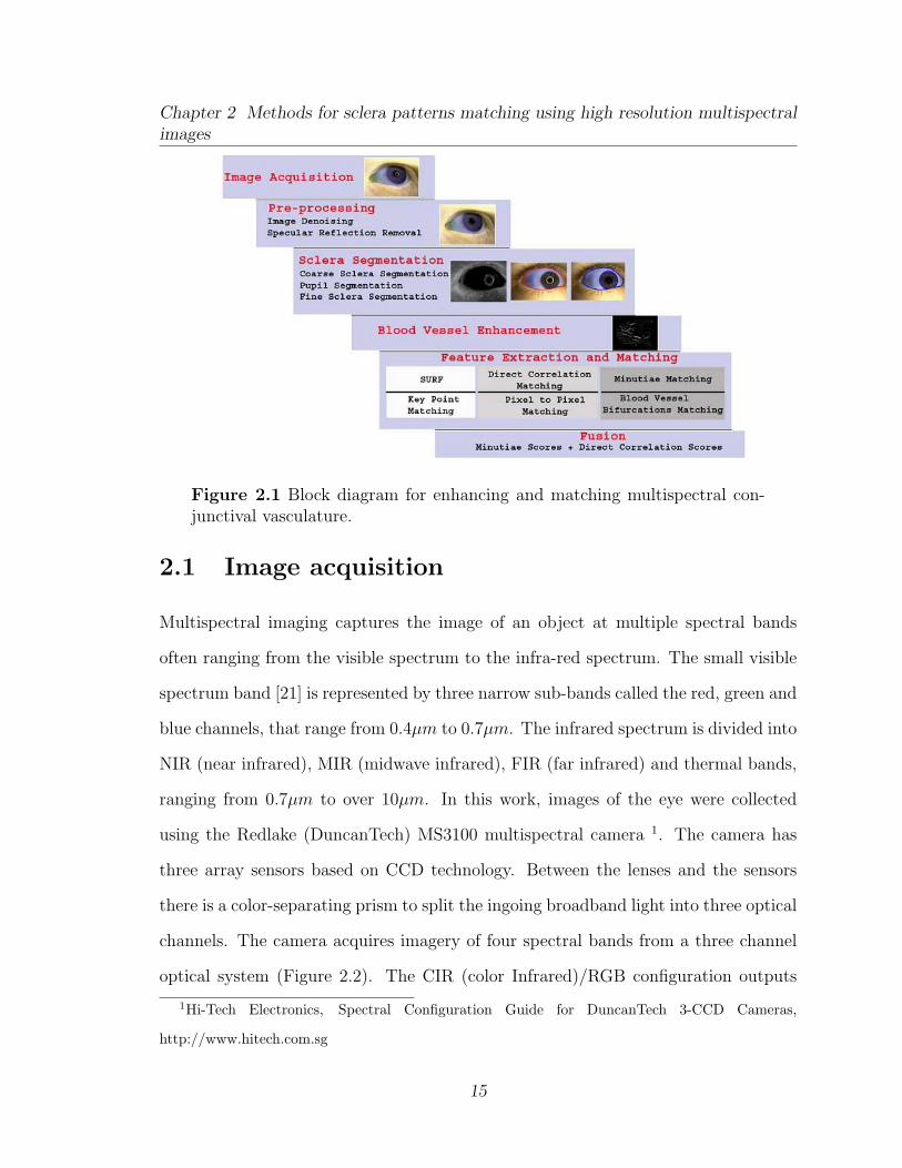
2.1 Block diagram for enhancing and matching multispectral conjunctivalvasculature. . . . . . . . . . . . . . . . . . . . . . . . . . . . . . . . . 15
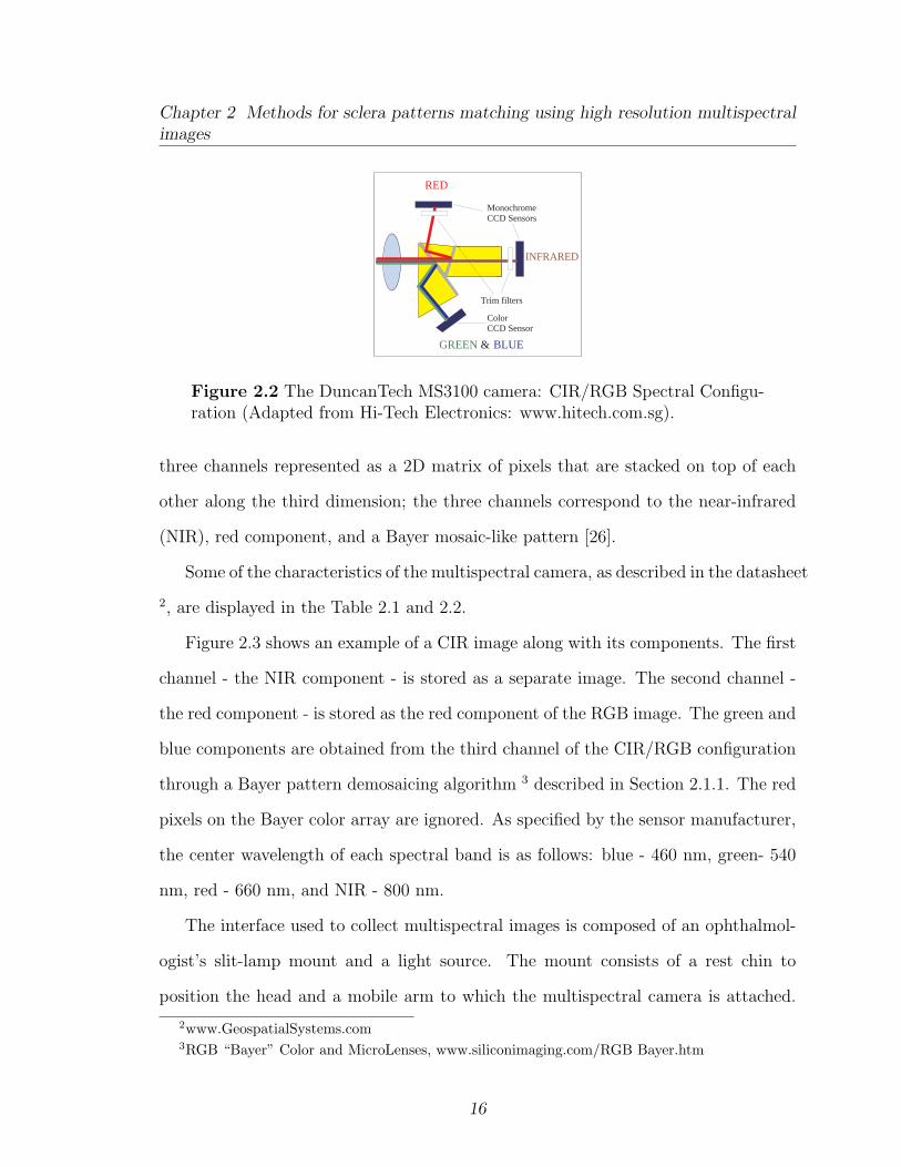
2.2 The DuncanTech MS3100 camera: CIR/RGB Spectral Configuration(Adapted from Hi-Tech Electronics: www.hitech.com.sg). . . . . . . . 16
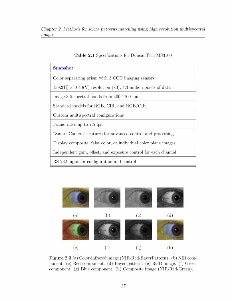
2.3 (a) Color-infrared image (NIR-Red-BayerPattern). (b) NIR compo-nent. (c) Red component. (d) Bayer pattern. (e) RGB image. (f)Green component. (g) Blue component. (h) Composite image (NIR-Red-Green). . . . . . . . . . . . . . . . . . . . . . . . . . . . . . . . . 17
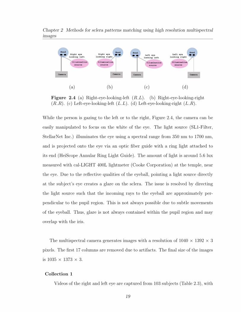
2.4 (a) Right-eye-looking-left (R L). (b) Right-eye-looking-right (R R).(c) Left-eye-looking-left (L L). (d) Left-eye-looking-right (L R). . . . 19
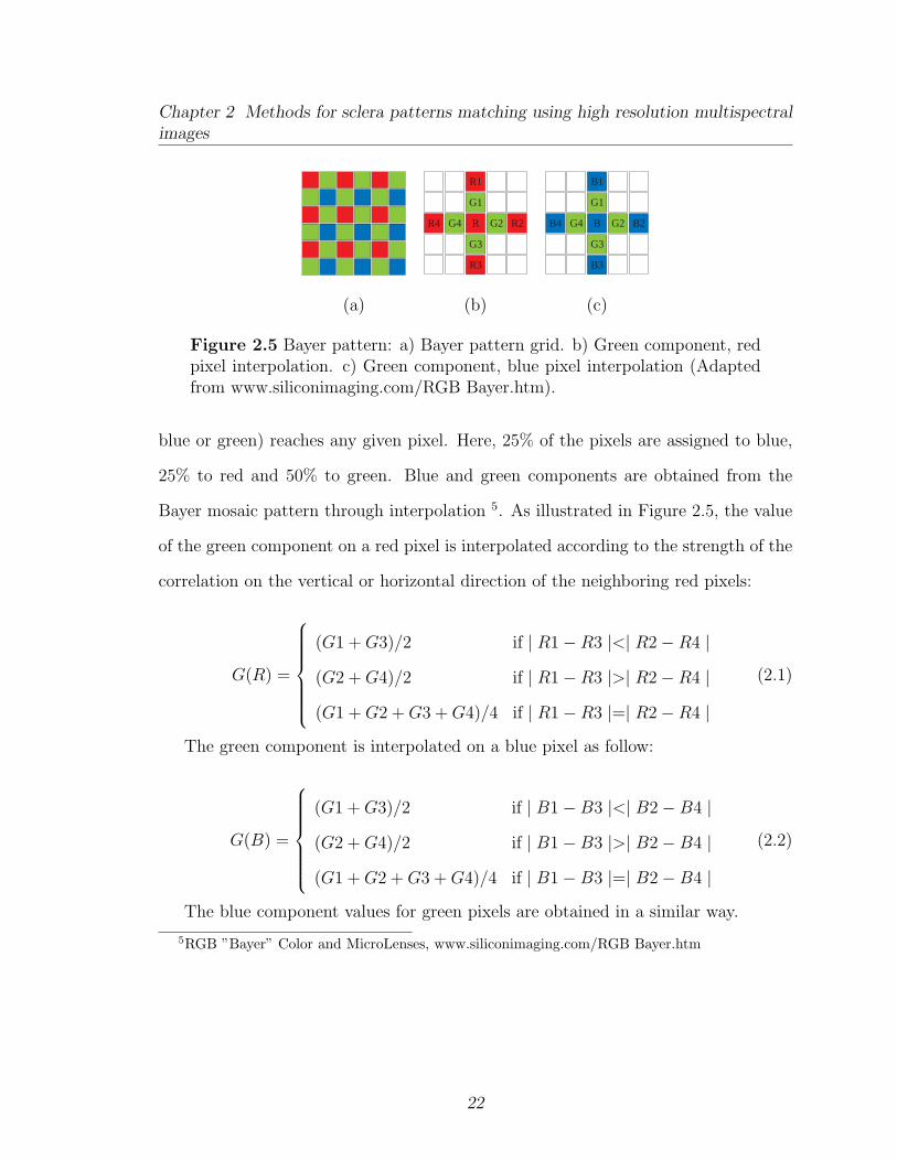
2.5 Bayer pattern: a) Bayer pattern grid. b) Green component, red pixelinterpolation. c) Green component, blue pixel interpolation (Adaptedfrom www.siliconimaging.com/RGB Bayer.htm). . . . . . . . . . . . . 22
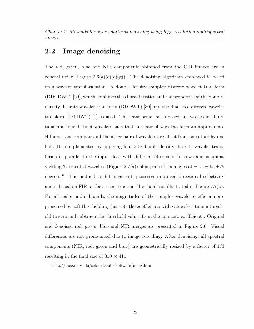
2.6 Denoising with Double Density Complex Discrete Wavelet Transform.a) Original NIR. b) Denoised NIR. c) Original red component. d)Denoised red component. e) Original green component. f) Denoisedgreen component. g) Original blue component. h) Denoised blue com-ponent. Visual differences between original and denoised images arenot pronounced due to image rescaling. . . . . . . . . . . . . . . . . . 24
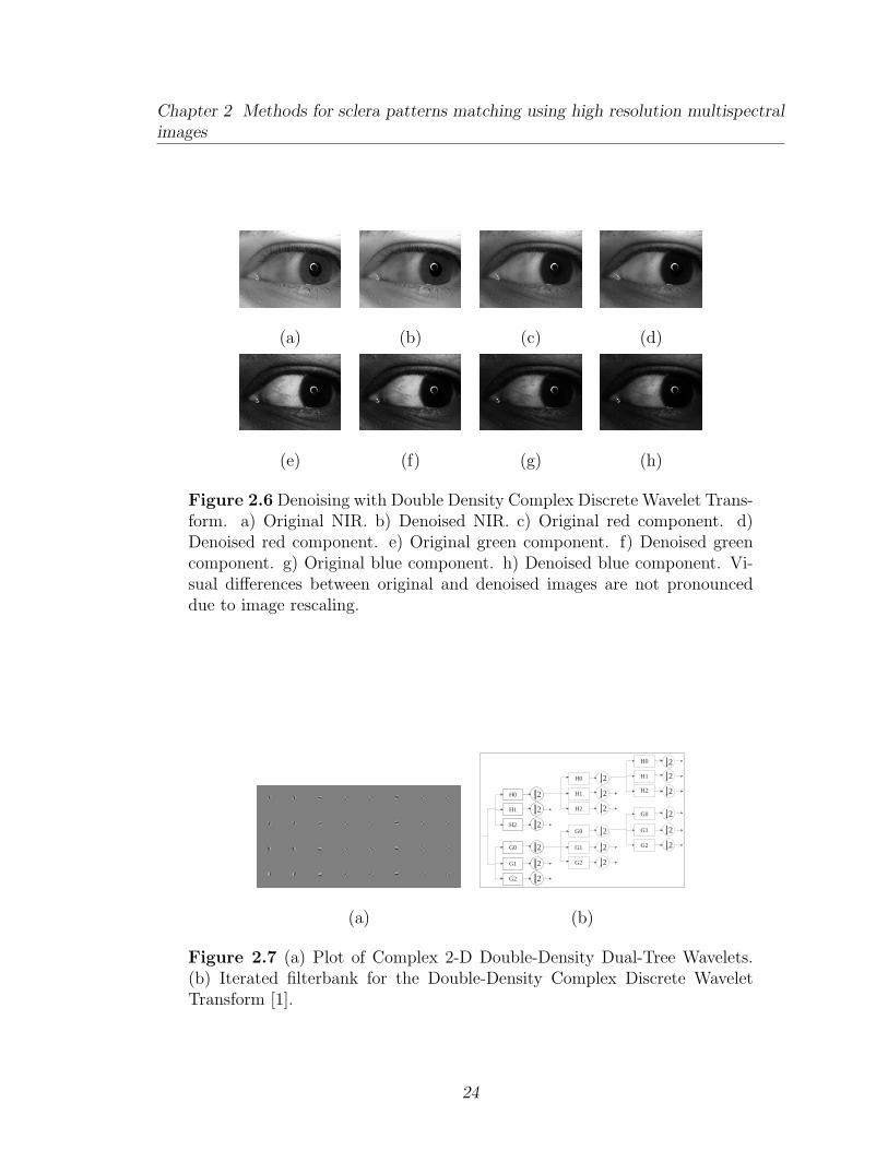
2.7 (a) Plot of Complex 2-D Double-Density Dual-Tree Wavelets. (b) It-erated filterbank for the Double-Density Complex Discrete WaveletTransform [1]. . . . . . . . . . . . . . . . . . . . . . . . . . . . . . . . 24
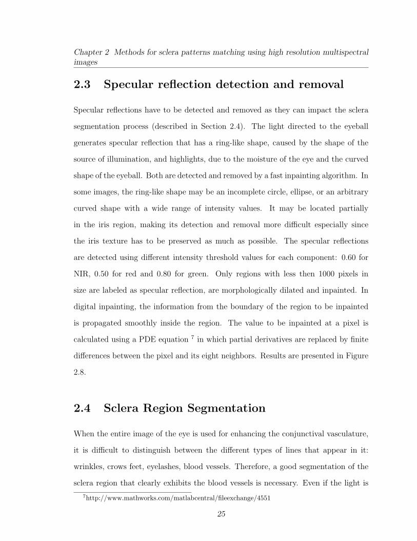
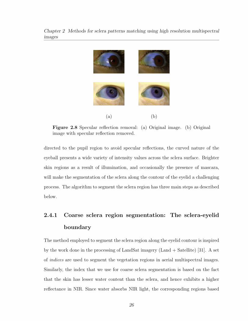
2.8 Specular reflection removal: (a) Original image. (b) Original imagewith specular reflection removed. . . . . . . . . . . . . . . . . . . . . 26
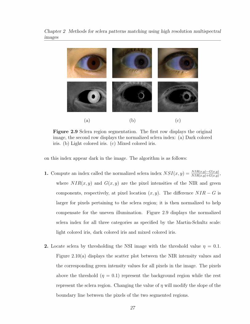
2.9 Sclera region segmentation. The first row displays the original image,the second row displays the normalized sclera index: (a) Dark colorediris. (b) Light colored iris. (c) Mixed colored iris. . . . . . . . . . . . 27
viii

LIST OF FIGURES
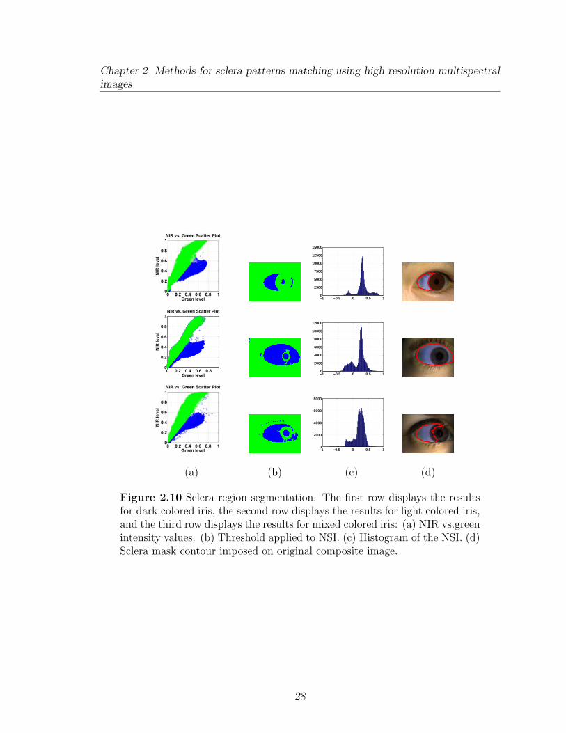
2.10 Sclera region segmentation. The first row displays the results for darkcolored iris, the second row displays the results for light colored iris,and the third row displays the results for mixed colored iris: (a) NIRvs.green intensity values. (b) Threshold applied to NSI. (c) Histogramof the NSI. (d) Sclera mask contour imposed on original composite image. 28
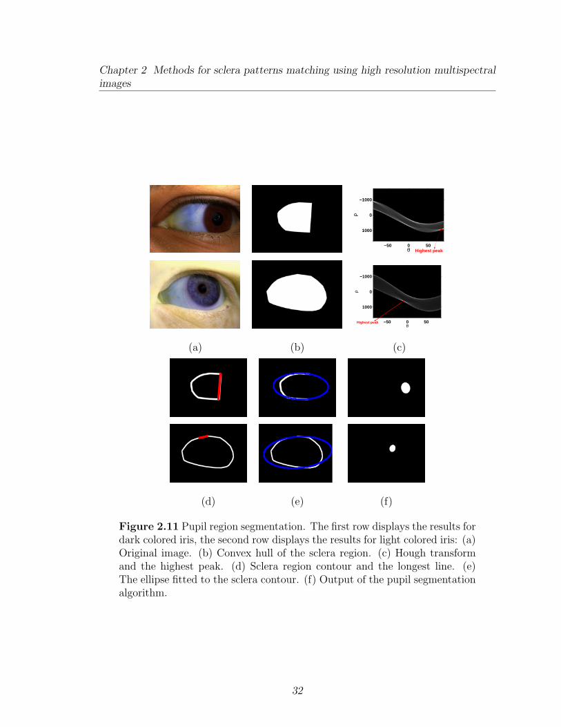
2.11 Pupil region segmentation. The first row displays the results for darkcolored iris, the second row displays the results for light colored iris:(a) Original image. (b) Convex hull of the sclera region. (c) Houghtransform and the highest peak. (d) Sclera region contour and thelongest line. (e) The ellipse fitted to the sclera contour. (f) Output ofthe pupil segmentation algorithm. . . . . . . . . . . . . . . . . . . . . 32
2.12 Sclera region segmentation.The first row displays the contour of thesclera cluster and pupil mask, the second row displays the Contour ofthe convex hull of the sclera cluster and pupil mask imposed on thecomposite image ISIP . (a) Dark colored iris. (b) Light colored iris. (c)Mixed colored iris. . . . . . . . . . . . . . . . . . . . . . . . . . . . . 33
2.13 Sclera region segmentation. The first row displays the results for darkcolored iris, the second row displays the results for light colored iris,and the third row displays the results for mixed colored iris: (a) Greencomponent. (b) Red Component. (c) Proportion of sclera in northdirection p↑(x, y). (d) Proportion of sclera in south direction p↓(x, y).(e) The proportion of sclera in east direction p←(x, y) for left gazedirection. . . . . . . . . . . . . . . . . . . . . . . . . . . . . . . . . . 34
2.14 Sclera region segmentation. The first row displays the K-means output,the second row displays Contour of the segmented sclera mask imposedon the composite image: (a) Dark colored iris. (b) Light colored iris.(c)Mixed colored iris. . . . . . . . . . . . . . . . . . . . . . . . . . . . . 36
2.15 Example of eye images with: (a) Plenty of mascara. (b) Improperillumination. . . . . . . . . . . . . . . . . . . . . . . . . . . . . . . . . 36
2.16 Failure to remove the proper line using Hough transform: (a) Correctdetection of the longest line. (b) Incorrect detection of the longest line. 37
2.17 Blood vessel enhancement on the segmented sclera region. (a) Greencomponent of the segmented sclera. (b) Result of the enhancement ofblood vessels. (c) The complement image of the enhanced blood vessels 38
2.18 Image registration of the sclera region from images of the same eye. a)Source image. b) Target image. c) Registered source. d) Flow imagedepicting the warping process. e) Estimated contrast map . . . . . . 40
2.19 Image registration of the sclera region from two different eyes. a)Source image. b) Target image. c) Registered source. d) Flow im-age depicting the warping process. e) Estimated contrast map. . . . . 41
ix
LIST OF FIGURES
2.20 The output of the SURF algorithm when applied to enhanced bloodvessel images of the same eye (The complement of the enhanced bloodvessel images are displayed for better visualization). The number ofinterest points: 112 and 108. (a) The first 10 pairs of correspondinginterest points. (b) All the pairs of corresponding interest points. . . 43
2.21 The output of the SURF algorithm when applied to enhanced bloodvessel images of different eyes (The complement of the enhanced bloodvessel images are displayed for better visualization). Number of interestpoints: 112 and 64. (a) The first 10 pairs of corresponding interestpoints. (b) All the pairs of corresponding interest points. . . . . . . . 44
2.22 The centerline of the segmented blood vessels imposed on the greencomponent of two images. . . . . . . . . . . . . . . . . . . . . . . . . 45
2.23 Detection of minutiae points. (a) Enhanced blood vessels image. (b)Centerline of the detected blood vessels. (c) Minutiae points: bifurca-tions (red) and endings (green). . . . . . . . . . . . . . . . . . . . . . 46
2.24 Failure to detect minutiae points. (a) Enhanced blood vessels image.(b) The detected vasculature without ramifications and intersections(Morphological operations such as dilation is applied to the blood ves-sels for a better visualization). . . . . . . . . . . . . . . . . . . . . . . 46
2.25 The histogram (25 bins) of the detected number of interest points forimages of the eye (data collection 1). (a) Left-eye-looking-left (L L).(b) Left-eye-looking-right (L R). (c) Right-eye-looking-right (R L). (d)Right-eye-looking-right (R R) . . . . . . . . . . . . . . . . . . . . . . 48
3.1 Block Diagram . . . . . . . . . . . . . . . . . . . . . . . . . . . . . . 553.2 The sclera-eyelid boundary. The first row displays the results for dark
colored iris, the second row displays the results for light colored iris,and the third row displays the results for mix colored iris: (a) originalcomposite image. (b) The normalized sclera index (NSI). (c) The out-put of the K-means clustering algorithm. (d) Sclera-eyelid boundaryimposed on original composite image. . . . . . . . . . . . . . . . . . . 59
3.3 The sclera-eyelid boundary errors. First row represents the errors inimages with strong uneven illumination. Second row represents theerrors in images with large specular reflections on the skin. (a) Originalcomposite image. (b) Normalized sclera index. (c) The output of thek-means algorithm. . . . . . . . . . . . . . . . . . . . . . . . . . . . . 61
3.4 Pupil region segmentation. Filling the holes at the iris-pupil boundarydue to inpainting of the specular reflection that results in higher pixelvalue than the pupil pixel value. . . . . . . . . . . . . . . . . . . . . . 62
x
LIST OF FIGURES
3.5 Pupil region segmentation. (a) The metric M for the thresholds 0.04,0.1, and 0.16. (b) Thresholding result (the contour) imposed on thecomposite image, thresholds 0.04, 0.1, and 0.16. (c) The metric Mfor the thresholds 0.18, 0.2, and 0.24. (d) Thresholding result (thecontour) imposed on the composite image, for thresholds 0.18, 0.2,and 0.24. . . . . . . . . . . . . . . . . . . . . . . . . . . . . . . . . . . 64
3.6 Pupil region segmentation. Examples. . . . . . . . . . . . . . . . . . . 643.7 Ocular images with a greater amount of melanin around the iris region. 653.8 Iris segmentation. Elliptical unwrapping based on the pupil parame-
ters: (a)Dark colored iris . (b) Light colored iris . (c) Mixed colorediris. . . . . . . . . . . . . . . . . . . . . . . . . . . . . . . . . . . . . . 69
3.9 Iris segmentation.The first row displays the results for dark colored iris,the second row displays the results for light colored iris, and the thirdrow displays the results for mix colored iris: (a) Pupil mask unwrapped.(b) Sclera mask unwrapped. . . . . . . . . . . . . . . . . . . . . . . . 69
3.10 Iris segmentation. Contour of the two ellipses, Ellipsemin and Ellipsemax,and their tilt imposed on the composite image. . . . . . . . . . . . . . 70
3.11 Iris segmentation: (a) Color gradient on composite image. (b) Thethreshold and Ellipsemax ellipse mask imposed on color gradient imageColorGradTh. . . . . . . . . . . . . . . . . . . . . . . . . . . . . . . . 70
3.12 Iris segmentation. Image ColorGradTh unwrapped along with the twolines Boundarysimin (red color) and Boundarysimax (blue color). . . . 71
3.13 Examples of segmented irides: (a) Dark colored iris. (b) Light colorediris. (c) Mixed colored iris. . . . . . . . . . . . . . . . . . . . . . . . . 71
3.14 Examples of correct eye image segmentation. . . . . . . . . . . . . . . 723.15 Examples of correct eye image segmentation. . . . . . . . . . . . . . . 723.16 Iris normalization: Daugman rubber sheet model. . . . . . . . . . . . 743.17 Examples for iris normalization: (a) Normalized iris. (b) The mask for
occlusions. . . . . . . . . . . . . . . . . . . . . . . . . . . . . . . . . . 743.18 Gabor wavelet . . . . . . . . . . . . . . . . . . . . . . . . . . . . . . . 753.19 Phase quantization: (a) Four levels represented by the sign of the Im
and Re for every quadrant (0 - negative, 1 - positive). (b) Example ofiris template. . . . . . . . . . . . . . . . . . . . . . . . . . . . . . . . 76
4.1 Block Diagram . . . . . . . . . . . . . . . . . . . . . . . . . . . . . . 82
5.1 Near images of the eye where the subject is: a) looking straight ahead,b) looking up, c) looking left, d) looking right. . . . . . . . . . . . . . 89
5.2 Segmenting the sclera from two different eye images, displayed by col-umn: a) Original image, b) Segmented sclera region based on RGBvalues (red = sclera region, blue = iris region, black = the background)c) Convex hull of the sclera (blue+red) containing a portion of the iris(blue) . . . . . . . . . . . . . . . . . . . . . . . . . . . . . . . . . . . 90
xi

LIST OF FIGURES
5.3 Segmenting the sclera of two different eye images: a) Original image,b) Sclera mask, c) Segmented sclera region. . . . . . . . . . . . . . . . 90
5.4 Plots of the equation 5.1 for various values of γ; c = 1 in all cases . . 925.5 Detection of specularities. Examples for γ = 3: (a) Illumination com-
ponent of HSI sclera image; (b) Histogram of the illumination compo-nent; (c) Filtered envelop of the histogram . . . . . . . . . . . . . . . 94
5.6 Example of threshold values for different values of γ . . . . . . . . . . 945.7 Detecting specularities: a) Original image, b) Threshold values for
1 ≤ γ ≤ 10 c) Specular reflection mask . . . . . . . . . . . . . . . . . 945.8 Segmenting the sclera after removing specularities: a) Original image,
b) Specular reflection mask c) Segmented sclera without specular re-flection . . . . . . . . . . . . . . . . . . . . . . . . . . . . . . . . . . . 95
5.9 Image Enhancement:(a) Original sclera vein image, (b) Enhanced scleravein image. . . . . . . . . . . . . . . . . . . . . . . . . . . . . . . . . 96
5.10 Example of pre-processed sclera vein image. . . . . . . . . . . . . . . 965.11 ROC curve indicating the results of matching . . . . . . . . . . . . . 97
A.1 Data collection 1. The ROC and the distribution of scores for theSURF technique. . . . . . . . . . . . . . . . . . . . . . . . . . . . . . 106
A.2 Data collection 1. The ROC and the distribution of scores for theminutiae-based matching technique. . . . . . . . . . . . . . . . . . . . 107
A.3 Data collection 1. The ROC and the distribution of scores for thecorrelation technique. . . . . . . . . . . . . . . . . . . . . . . . . . . . 108
A.4 Data collection 1. The ROC and the distribution of scores for themutual information technique. . . . . . . . . . . . . . . . . . . . . . . 109
A.5 Data collection 1. The ROC and the distribution of scores for thenormalized mutual information technique. . . . . . . . . . . . . . . . 110
A.6 Data collection 1. The ROC and the distribution of scores for theratio-image uniformity technique. . . . . . . . . . . . . . . . . . . . . 111
A.7 Data collection 1. The ROC and the distribution of scores for the rootmean square error technique. . . . . . . . . . . . . . . . . . . . . . . . 112
A.8 Data collection 1. The ROC and the distribution of scores for thestructural similarity index technique. . . . . . . . . . . . . . . . . . . 113
A.9 Data collection 1. The ROC and the distribution of scores for thefusion of minutiae and correlation technique. . . . . . . . . . . . . . . 114
A.10 Data collection 1. The ROC and the distribution of scores for thefusion of minutiae and mutual information technique. . . . . . . . . . 115
A.11 Data collection 1. The ROC and the distribution of scores for thefusion of minutiae and normalized mutual information technique. . . 116
A.12 Data collection 1. The ROC and the distribution of scores for thefusion of minutiae and ratio-image uniformity technique. . . . . . . . 117
A.13 Data collection 1. The ROC and the distribution of scores for thefusion of minutiae and root mean square error technique. . . . . . . . 118
xii

LIST OF FIGURES
A.14 Data collection 1. The ROC and the distribution of scores for thefusion of minutiae and structural similarity index technique. . . . . . 119
B.1 Data collection 1. The ROC and the distribution of scores for theSURF technique (automatic sclera segmentation). . . . . . . . . . . . 121
B.2 Data collection 1. The ROC and the distribution of scores for theHamming distance. . . . . . . . . . . . . . . . . . . . . . . . . . . . . 122
B.3 Data collection 1. Fusion of iris patterns and sclera patterns. The ROCand the distribution of scores for L L, simple sum rule, maximum rule,minimum rule. . . . . . . . . . . . . . . . . . . . . . . . . . . . . . . . 123
B.4 Data collection 1. Fusion of iris patterns and sclera patterns. The ROCand the distribution of scores for L R, simple sum rule, maximum rule,minimum rule. . . . . . . . . . . . . . . . . . . . . . . . . . . . . . . . 124
B.5 Data collection 1. Fusion of iris patterns and sclera patterns. The ROCand the distribution of scores for R L, simple sum rule, maximum rule,minimum rule. . . . . . . . . . . . . . . . . . . . . . . . . . . . . . . . 125
B.6 Data collection 1. Fusion of iris patterns and sclera patterns. The ROCand the distribution of scores for R R, simple sum rule, maximum rule,minimum rule. . . . . . . . . . . . . . . . . . . . . . . . . . . . . . . . 126
C.1 Data collection 2. The ROC and the distribution of scores for theSURF technique. . . . . . . . . . . . . . . . . . . . . . . . . . . . . . 128
C.2 Data collection 2. The ROC and the distribution of scores for theminutiae-based matching technique. . . . . . . . . . . . . . . . . . . . 129
C.3 Data collection 2. The ROC and the distribution of scores for thecorrelation technique. . . . . . . . . . . . . . . . . . . . . . . . . . . . 130
C.4 Data collection 2. The ROC and the distribution of scores for themutual information technique. . . . . . . . . . . . . . . . . . . . . . . 131
C.5 Data collection 2. The ROC and the distribution of scores for thenormalized mutual information technique. . . . . . . . . . . . . . . . 132
C.6 Data collection 2. The ROC and the distribution of scores for theratio-image uniformity technique. . . . . . . . . . . . . . . . . . . . . 133
C.7 Data collection 2. The ROC and the distribution of scores for the rootmean square error technique. . . . . . . . . . . . . . . . . . . . . . . . 134
C.8 Data collection 2. The ROC and the distribution of scores for thestructural similarity index technique. . . . . . . . . . . . . . . . . . . 135
C.9 Data collection 2. The ROC and the distribution of scores for theHamming distance. . . . . . . . . . . . . . . . . . . . . . . . . . . . . 136
C.10 Data collection 2. The fusion of iris and sclera patterns for left-eye-looking-left. The ROC and the distribution of scores. . . . . . . . . . 137
C.11 Data collection 2. The fusion of iris and sclera patterns for left-eye-looking-right. The ROC and the distribution of scores. . . . . . . . . 138
xiii

LIST OF FIGURES
C.12 Data collection 2. The fusion of iris and sclera patterns for right-eye-looking-left. The ROC and the distribution of scores. . . . . . . . . . 139
C.13 Data collection 2. The fusion of iris and sclera patterns for right-eye-looking-right. The ROC and the distribution of scores. . . . . . . . . 140
xiv
List of Tables
2.1 Specifications for DuncanTech MS3100 . . . . . . . . . . . . . . . . . 172.2 Performance specifications for DuncanTech MS3100 . . . . . . . . . . 182.3 High resolution multispectral database . . . . . . . . . . . . . . . . . 212.4 The EER (%) results when using SURF. . . . . . . . . . . . . . . . . 492.5 The average number of detected interest points for data collection 1 . 492.6 The EER (%) results when using minutiae points. . . . . . . . . . . . 492.7 The EER (%) results when using different correlation methods. . . . 502.8 The EER (%) results of the fusion of minutiae scores with different
correlation measures. . . . . . . . . . . . . . . . . . . . . . . . . . . . 52
3.1 The EER (%) results for iris patterns using Hamming distance. . . . 783.2 The EER (%) results for scleral patterns when using SURF. . . . . . 783.3 The EER (%) results of the fusion of iris patterns (Hamming distance)
and scleral patterns (SURF). . . . . . . . . . . . . . . . . . . . . . . . 793.4 Average computation times . . . . . . . . . . . . . . . . . . . . . . . 79
4.1 The EER (%) results for scleral patterns when using SURF. . . . . . 844.2 The EER (%) results for scleral patterns when using minutiae points. 844.3 The EER (%) results for scleral patterns when using different correla-
tion methods. . . . . . . . . . . . . . . . . . . . . . . . . . . . . . . . 854.4 The EER (%) results for iris patterns using Hamming distance. . . . 864.5 The EER (%) results of the fusion of iris patterns (Hamming distance)
and scleral patterns (SURF). . . . . . . . . . . . . . . . . . . . . . . . 86
5.1 Manual correction statistics of segmented sclera . . . . . . . . . . . . 91
xv

Chapter 1
Introduction
Biometrics is the science of recognizing a person based on physical traits such as face,
fingerprint, and iris or behavioral characteristics such as gait, keystroke dynamics,
and signature [2]. Conventional techniques to authenticate an individual are based
on identification cards (something that you carry) and passwords or PINs (something
that you know). An issue associated with these ways of authentication is that the
cards, passwords and PINs can be stolen, lost, or simply forgotten. The need to
reliably determine and verify the identity of a person in a convenient, easy, and
accessible way has stimulated intense research in the field of biometric authentication.
Rooted in the latin word oculus that means eye, the term ocular biometrics is
used to bring together all the biometric modalities associated with the eye and its
surrounding region. Defined as an organ of sight, a specialized light-sensitive sensory
structure, the eye allow us to observe and learn about the surrounding world. A
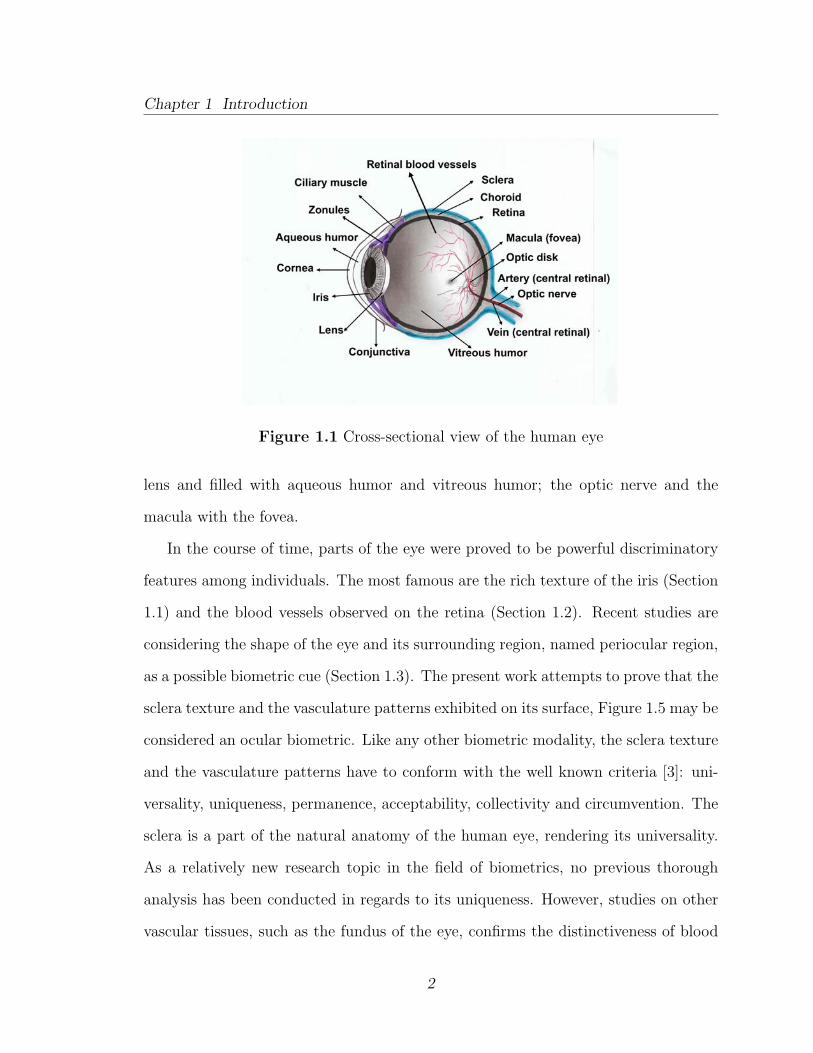
cross section (Figure 1.1) reveals the main parts of the eye: the extraocular muscles
that controls the movement of the eyeball within the eye socket; the three layers
surrounding the eyeball, the sclera, the choroid and the retina with the cornea, the
iris and conjunctiva in front; the anterior and posterior chambers separated by the
1
Chapter 1 Introduction
Figure 1.1 Cross-sectional view of the human eye
lens and filled with aqueous humor and vitreous humor; the optic nerve and the
macula with the fovea.
In the course of time, parts of the eye were proved to be powerful discriminatory
features among individuals. The most famous are the rich texture of the iris (Section
1.1) and the blood vessels observed on the retina (Section 1.2). Recent studies are
considering the shape of the eye and its surrounding region, named periocular region,
as a possible biometric cue (Section 1.3). The present work attempts to prove that the
sclera texture and the vasculature patterns exhibited on its surface, Figure 1.5 may be
considered an ocular biometric. Like any other biometric modality, the sclera texture
and the vasculature patterns have to conform with the well known criteria [3]: uni-
versality, uniqueness, permanence, acceptability, collectivity and circumvention. The
sclera is a part of the natural anatomy of the human eye, rendering its universality.
As a relatively new research topic in the field of biometrics, no previous thorough
analysis has been conducted in regards to its uniqueness. However, studies on other
vascular tissues, such as the fundus of the eye, confirms the distinctiveness of blood
2
Chapter 1 Introduction
vessel patterns, has provided evidence of the long lasting form of the vessels and their
durability through the years as age progresses. Outside factors such as exposure to
chemicals, physical trauma, and some diseases may influence the appearance of the
sclera region. Images of the sclera region are easily collected with commercial digital
cameras when a proper amount of light is directed towards the eye, and therefore it
can be easily photographed without intrusion and discomfort to the subject. Staring
at a specific point is not required, and only a fraction of a second is needed to capture
the image of the eye; the subject is not obligated to be stationary for long periods
of time. Reproducing the rich texture of the sclera region is difficult, making this
modality invulnerable to imitation and tampering.
1.1 Iris recognition
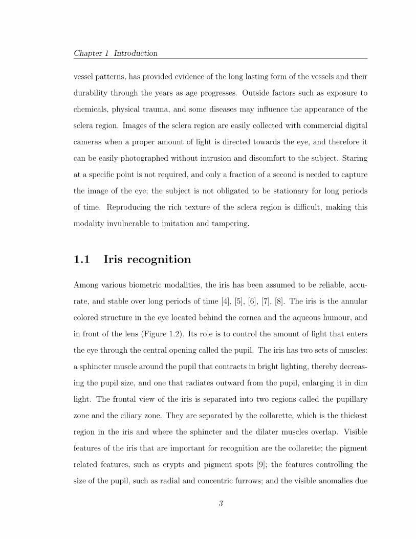
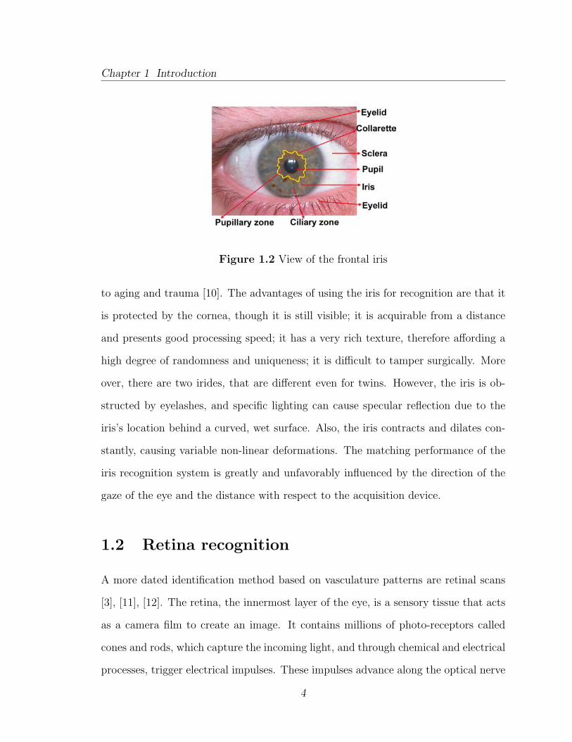
Among various biometric modalities, the iris has been assumed to be reliable, accu-
rate, and stable over long periods of time [4], [5], [6], [7], [8]. The iris is the annular
colored structure in the eye located behind the cornea and the aqueous humour, and
in front of the lens (Figure 1.2). Its role is to control the amount of light that enters
the eye through the central opening called the pupil. The iris has two sets of muscles:
a sphincter muscle around the pupil that contracts in bright lighting, thereby decreas-
ing the pupil size, and one that radiates outward from the pupil, enlarging it in dim
light. The frontal view of the iris is separated into two regions called the pupillary
zone and the ciliary zone. They are separated by the collarette, which is the thickest
region in the iris and where the sphincter and the dilater muscles overlap. Visible
features of the iris that are important for recognition are the collarette; the pigment
related features, such as crypts and pigment spots [9]; the features controlling the
size of the pupil, such as radial and concentric furrows; and the visible anomalies due
3
Chapter 1 Introduction
Figure 1.2 View of the frontal iris
to aging and trauma [10]. The advantages of using the iris for recognition are that it
is protected by the cornea, though it is still visible; it is acquirable from a distance
and presents good processing speed; it has a very rich texture, therefore affording a
high degree of randomness and uniqueness; it is difficult to tamper surgically. More
over, there are two irides, that are different even for twins. However, the iris is ob-
structed by eyelashes, and specific lighting can cause specular reflection due to the
iris’s location behind a curved, wet surface. Also, the iris contracts and dilates con-
stantly, causing variable non-linear deformations. The matching performance of the
iris recognition system is greatly and unfavorably influenced by the direction of the
gaze of the eye and the distance with respect to the acquisition device.
1.2 Retina recognition
A more dated identification method based on vasculature patterns are retinal scans
[3], [11], [12]. The retina, the innermost layer of the eye, is a sensory tissue that acts
as a camera film to create an image. It contains millions of photo-receptors called
cones and rods, which capture the incoming light, and through chemical and electrical
processes, trigger electrical impulses. These impulses advance along the optical nerve
4
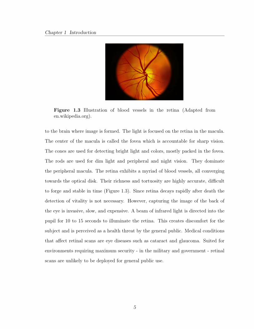
Chapter 1 Introduction
Figure 1.3 Illustration of blood vessels in the retina (Adapted fromen.wikipedia.org).
to the brain where image is formed. The light is focused on the retina in the macula.
The center of the macula is called the fovea which is accountable for sharp vision.
The cones are used for detecting bright light and colors, mostly packed in the fovea.
The rods are used for dim light and peripheral and night vision. They dominate
the peripheral macula. The retina exhibits a myriad of blood vessels, all converging
towards the optical disk. Their richness and tortuosity are highly accurate, difficult
to forge and stable in time (Figure 1.3). Since retina decays rapidly after death the
detection of vitality is not necessary. However, capturing the image of the back of
the eye is invasive, slow, and expensive. A beam of infrared light is directed into the
pupil for 10 to 15 seconds to illuminate the retina. This creates discomfort for the
subject and is perceived as a health threat by the general public. Medical conditions
that affect retinal scans are eye diseases such as cataract and glaucoma. Suited for
environments requiring maximum security - in the military and government - retinal
scans are unlikely to be deployed for general public use.
5

Chapter 1 Introduction
Figure 1.4 Periocular region
1.3 Periocular region
Recently, researchers explored the feasibility of using the periocular region, defined
as the region surrounding the eye, Figure 1.4, as a biometric cue [13], [14], [15]. The
periocular region’s role is significant when the eye is occluded (e.g., due to blinking).
Its advantages are that it can be captured without strict viewing angle and distance
constraints, and it does not necessarily require the subject’s cooperation. Eye shape
and skin texture encoded by local or global features can be used as soft biometrics [14].
A limitation of the periocular region is that the features are not as distinguishable as
iris, resulting in lower accuracy.
1.4 Sclera region
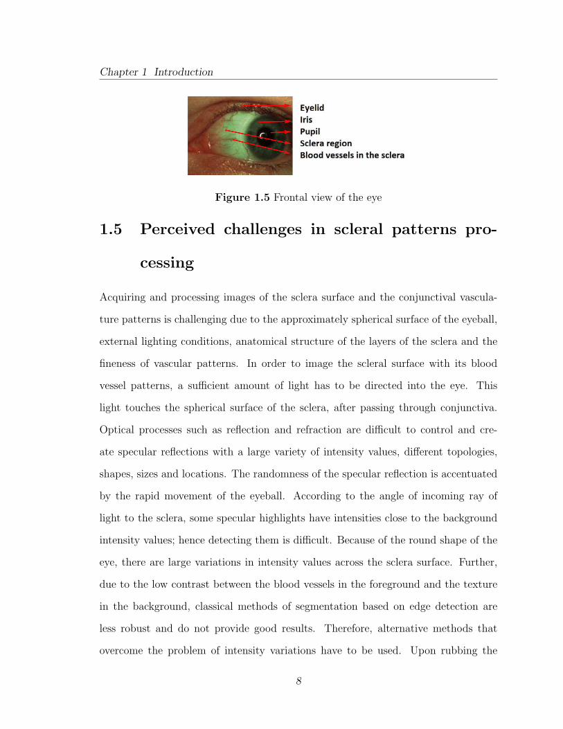
In contrast, visible on the sclera (the white of the eye), a structure of fine blood vessels
may be imaged without discomfort for the subject (Figure 1.5). These patterns,
composed of more or less prominent veins, are visible at all times, except when the
gaze direction is downward and the eye is covered by the eyelid. Their richness
is increased in non-frontal eye images, thus allowing the sclera region to be used
in addition to iris recognition for more complete and accurate identification. The
sclera [16], [17] is the external layer of the eye, a protective coat serving to maintain
6
Chapter 1 Introduction
the form of the eyeball under the pressure of the eye’s internal liquids. It also provides
an attachment for ligaments and the six extraocular muscles which rotate the eyeball
in the eye socket. It is a firm, dense membrane with thickness that varies from 0.8mm
to 0.3mm, containing collagen and elastic fibers. The sclera is organized in four layers
(from outermost to innermost): episclera, stroma, lamina fusca, and endothelium.
The sclera is generally avascular; only its outer surface, the episclera, contains the
blood vessels that nourish it. In the back of the eye, the sclera is continued with the
dural sheath of the optic nerve, and anterior sclera is completed by the cornea (a clear
and transparent layer at the center of the eye, located in front of the iris, and whose
main purpose is to focus the light as it enters the eye). The anterior part of the sclera,
up to the edge of the cornea (the sclero-corneal junction), and the inside of the eyelid,
are covered by the conjunctival membrane. The conjunctival membrane is a thin
layer containing secretory epithelium that helps lubricate the eye for eyelid closure
and protects the ocular surface from bacterial and viral infections. The part of the
conjunctiva that covers the inner lining of the eyelids is called palpebral conjunctiva.
The part of the conjunctiva that covers the outer surface of the eyeball is called bulbar
conjunctiva and the area where palpebral conjunctiva becomes the bulbar conjunctiva
is called the conjunctival fornix. The conjunctiva is semitransparent, colorless, and
contains blood vessels. Anatomically, the blood vessels in bulbar conjunctiva can be
differentiated from those of the episclera. While the conjunctival blood vessels can
slightly move with the conjunctival membrane, those in episclera will not [18]. The
rich vasculature patterns revealed in the episclera and conjunctival membrane are
together referred to as conjunctival vasculature in this study.
7
Chapter 1 Introduction
Figure 1.5 Frontal view of the eye
1.5 Perceived challenges in scleral patterns pro-
cessing
Acquiring and processing images of the sclera surface and the conjunctival vascula-
ture patterns is challenging due to the approximately spherical surface of the eyeball,
external lighting conditions, anatomical structure of the layers of the sclera and the
fineness of vascular patterns. In order to image the scleral surface with its blood
vessel patterns, a sufficient amount of light has to be directed into the eye. This
light touches the spherical surface of the sclera, after passing through conjunctiva.
Optical processes such as reflection and refraction are difficult to control and cre-
ate specular reflections with a large variety of intensity values, different topologies,
shapes, sizes and locations. The randomness of the specular reflection is accentuated
by the rapid movement of the eyeball. According to the angle of incoming ray of
light to the sclera, some specular highlights have intensities close to the background
intensity values; hence detecting them is difficult. Because of the round shape of the
eye, there are large variations in intensity values across the sclera surface. Further,
due to the low contrast between the blood vessels in the foreground and the texture
in the background, classical methods of segmentation based on edge detection are
less robust and do not provide good results. Therefore, alternative methods that
overcome the problem of intensity variations have to be used. Upon rubbing the
8
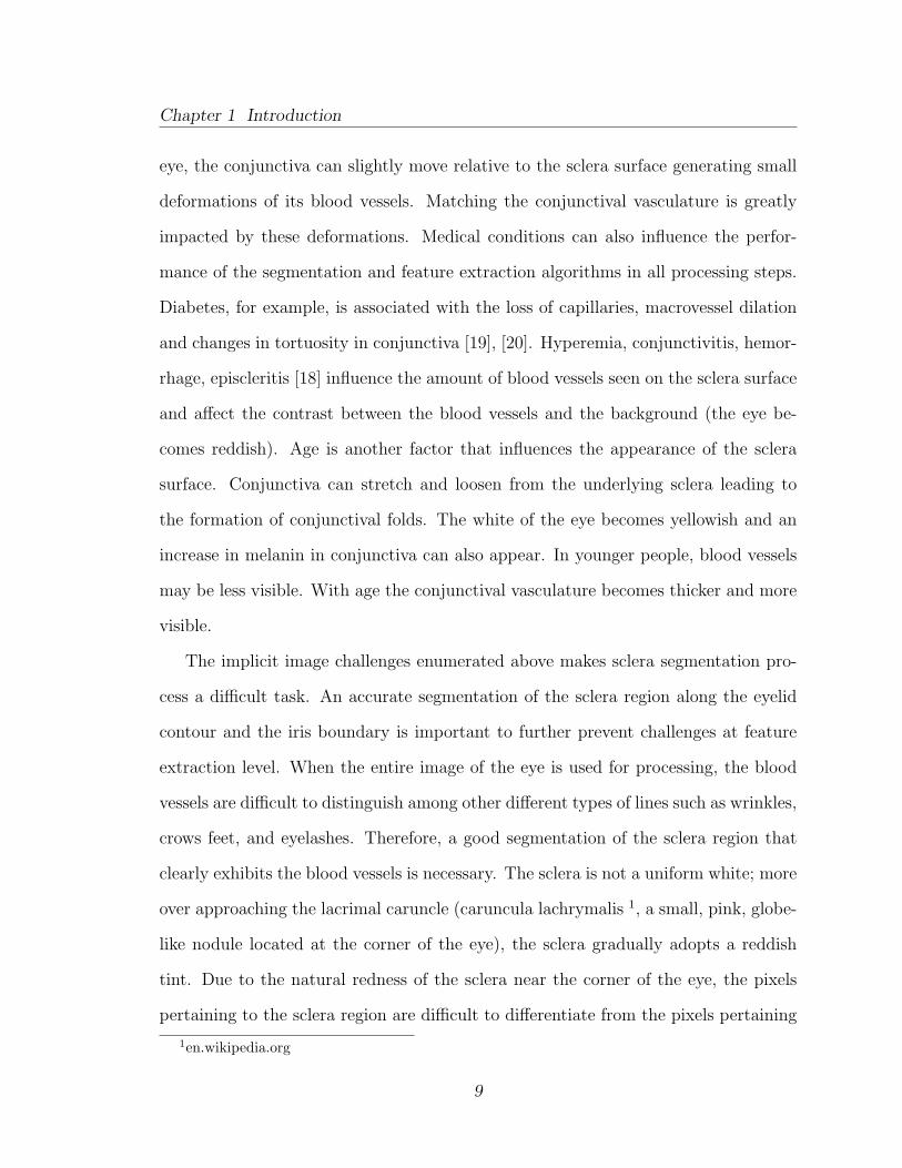
Chapter 1 Introduction
eye, the conjunctiva can slightly move relative to the sclera surface generating small
deformations of its blood vessels. Matching the conjunctival vasculature is greatly
impacted by these deformations. Medical conditions can also influence the perfor-
mance of the segmentation and feature extraction algorithms in all processing steps.
Diabetes, for example, is associated with the loss of capillaries, macrovessel dilation
and changes in tortuosity in conjunctiva [19], [20]. Hyperemia, conjunctivitis, hemor-
rhage, episcleritis [18] influence the amount of blood vessels seen on the sclera surface
and affect the contrast between the blood vessels and the background (the eye be-
comes reddish). Age is another factor that influences the appearance of the sclera
surface. Conjunctiva can stretch and loosen from the underlying sclera leading to
the formation of conjunctival folds. The white of the eye becomes yellowish and an
increase in melanin in conjunctiva can also appear. In younger people, blood vessels
may be less visible. With age the conjunctival vasculature becomes thicker and more
visible.
The implicit image challenges enumerated above makes sclera segmentation pro-
cess a difficult task. An accurate segmentation of the sclera region along the eyelid
contour and the iris boundary is important to further prevent challenges at feature
extraction level. When the entire image of the eye is used for processing, the blood
vessels are difficult to distinguish among other different types of lines such as wrinkles,
crows feet, and eyelashes. Therefore, a good segmentation of the sclera region that
clearly exhibits the blood vessels is necessary. The sclera is not a uniform white; more
over approaching the lacrimal caruncle (caruncula lachrymalis 1, a small, pink, globe-
like nodule located at the corner of the eye), the sclera gradually adopts a reddish
tint. Due to the natural redness of the sclera near the corner of the eye, the pixels
pertaining to the sclera region are difficult to differentiate from the pixels pertaining
1en.wikipedia.org
9

Chapter 1 Introduction
to the skin. Also, an improper illumination of the curved surface of the eye, may
result in darker regions in the corner of the eye opposite to lacrimal caruncle. These
issues create problems for the segmentation process.
The thresholding and clustering methods (k-means) for segmentation are employed
in the presented work with some degree of performance. The key in thresholding
method is to select the proper threshold [21]. A common threshold that is optimal
for the segmentation of the sclera in all the images is difficult to find. When the
clustering method k-means is used, the final solution depends largely on the initial
set of clusters. The algorithm is fast but does not guarantee a good sclera-eyelid
contour detection.
The histogram-based segmentation method [22] consists of finding the peaks and
valleys in the chart in order to locate clusters. The image of the eye is divided in
four regions of interest: the iris; the sclera; the skin and the pupil, eyelashes included.
This method is fast; it takes one pass to read the intensity value of the pixels and
to create the histogram. However, it is difficult to identify which peaks (clusters)
and valleys (the boundaries between the regions of interest) are significant. The four
clusters often overlap, meaning they are undistinguishable.
Boundaries between regions that are to be segmented are characterized by changes
in the intensity value of pixels. They are known as edges. There are many different
ways in which edges can be detected [23], [21], [22]. Unfortunately, these methods
result in a multitude of disconnected segments from which it is difficult to select the
proper boundaries of the sclera region. It is also challenging and problematic to con-
tinue the gaps along the contour between the sclera and the eyelids.
Region growing, and split-and merge methods [21] were employed without satis-
factory results due to the large variation is intensity values across the sclera region.
There are other algorithms that could potentially be used to segment the sclera region
10
Chapter 1 Introduction
such as partial differential equations (level set), graph partitioning and many others.
The image of the iris is better discerned in near infrared (NIR) spectrum, while
vasculature patterns are better observed in the visible spectrum (RGB). Therefore,
multispectral images of the eye (Section 2.1), consisting of both NIR and RGB chan-
nels, were used in this work in order to ensure that both the iris and the vasculature
patterns are successfully imaged. This dissertation is the first extensive work and
first attempt to demonstrate the validity of using the sclera texture and the con-
junctival vasculature visible on its surface as a new biometric modality. This idea
came to reality with the submission of Dr. R. Derakhshani’s and Dr. Arun Ross’
patent [24]. This work include the following enumerated contributions. Firstly, a
multispectral ocular database (2 collections of 103 and 31 subjects) was assembled
by collecting high-resolution color infrared images of the left and right eye using the
DuncanTech MS3100 multispectral camera under constrained conditions (Chapter 2).
Secondly, a novel segmentation algorithm was designed to localize the spatial extent
of the iris, sclera and pupil in the ocular images. The proposed segmentation al-
gorithm is a combination of region-based and edge-based schemes that exploits the
multispectral information (Chapter 2, 3). Thirdly, different feature extraction and
matching methods were used to determine the potential of utilizing the sclera and
the accompanying vasculature pattern as biometric cues. The three specific matching
methods considered in this work were keypoint-based matching, direct correlation
matching, and minutiae based on blood vessel bifurcations (Chapter 2, 4). Fourthly,
the potential of designing a bimodal ocular system that combines the sclera biometric
with the iris biometric was explored (Chapter 3, 4). It is well demonstrated that iris
recognition performance is greatly and negatively influenced by the occlusions, the
lighting conditions and by the direction of the gaze of the eye with respect to the
acquisition device [25]. The more the gaze direction deviates from the frontal pose,
11
Chapter 1 Introduction
the more information from the iris texture is lost and the more information from the
sclera region is gained. Depending on the richness and locality of the conjunctival
vasculature exposed on the surface of the sclera, prominent veins may be visible when
iris is occluded. More over, the combined sclera and the iris texture may be used in
non-cooperative recognition. In the attempt to establish the utility of the sclera re-
gion as a biometric cue, the analysis of the sclera surface is also considered in low
resolution, visible spectrum, unconstrained images. The purpose is to evaluate the
matching performance of the sclera texture and the blood vessels in each case and
to compare their performances when moving from high to low resolution images, and
changing the lighting conditions, acquiring distances and viewing angles (Chapter 5).
1.6 Summary
This chapter is an introduction to biometrics as a discipline. It presents the ocu-
lar biometric modalities, each with its advantages and disadvantages. Among these
modalities, iris recognition gained popularity in the last decade due to its reliability,
stability for long period of times and accuracy. However, the matching performance
of the iris recognition system is greatly and unfavorably influenced by the direction
of the gaze of the eye with respect to the acquisition device. To compensate the loss
of information in non-frontal images, the sclera texture and the blood vessels seen on
its surface are proposed as a new biometric modality to be combined with the iris
patterns. An anatomical introduction of the sclera is presented along with the per-
ceived challenges in scleral pattern processing. General segmentation methods used
with some degree of success to localize the sclera region are presented. The chapter
ends by enumerating the contributions of this work to initiate research in this field,
mainly to investigate the use of sclera texture and the conjunctival vasculature as a
12

Chapter 1 Introduction
biometric cue and the potential of designing a bimodal ocular system that combines
the scleral patterns with the iris patterns is proposed.
13
Chapter 2
Methods for sclera patterns
matching using high resolution
multispectral images
In order to prove the feasibility of using the sclera surface in an ocular biometric
system, it is essential to determine what features could be exploited for identifica-
tion, how powerful is their discriminatory potential, and what methods are the most
effective to characterize this biometric. In this dissertation, the design of three differ-
ent feature extraction and matching methods is presented. The first one is based on
interest-point detection and utilizes the entire sclera region including the vasculature
pattern; the second is based on minutiae points on the vasculature structure; and the
third is based on direct correlation. The block diagram of the proposed system is
shown in Figure 2.1. In this approach the multispectral collection 1 is used.
14
Chapter 2 Methods for sclera patterns matching using high resolution multispectralimages
Figure 2.1 Block diagram for enhancing and matching multispectral con-junctival vasculature.
2.1 Image acquisition
Multispectral imaging captures the image of an object at multiple spectral bands
often ranging from the visible spectrum to the infra-red spectrum. The small visible
spectrum band [21] is represented by three narrow sub-bands called the red, green and
blue channels, that range from 0.4µm to 0.7µm. The infrared spectrum is divided into
NIR (near infrared), MIR (midwave infrared), FIR (far infrared) and thermal bands,
ranging from 0.7µm to over 10µm. In this work, images of the eye were collected
using the Redlake (DuncanTech) MS3100 multispectral camera 1. The camera has
three array sensors based on CCD technology. Between the lenses and the sensors
there is a color-separating prism to split the ingoing broadband light into three optical
channels. The camera acquires imagery of four spectral bands from a three channel
optical system (Figure 2.2). The CIR (color Infrared)/RGB configuration outputs
1Hi-Tech Electronics, Spectral Configuration Guide for DuncanTech 3-CCD Cameras,
http://www.hitech.com.sg
15
Chapter 2 Methods for sclera patterns matching using high resolution multispectralimages
BLUE
Trim filters
Monochrome CCD Sensors
Color CCD Sensor
RED
INFRARED
GREEN &
Figure 2.2 The DuncanTech MS3100 camera: CIR/RGB Spectral Configu-ration (Adapted from Hi-Tech Electronics: www.hitech.com.sg).
three channels represented as a 2D matrix of pixels that are stacked on top of each
other along the third dimension; the three channels correspond to the near-infrared
(NIR), red component, and a Bayer mosaic-like pattern [26].
Some of the characteristics of the multispectral camera, as described in the datasheet
2, are displayed in the Table 2.1 and 2.2.
Figure 2.3 shows an example of a CIR image along with its components. The first
channel - the NIR component - is stored as a separate image. The second channel -
the red component - is stored as the red component of the RGB image. The green and
blue components are obtained from the third channel of the CIR/RGB configuration
through a Bayer pattern demosaicing algorithm 3 described in Section 2.1.1. The red
pixels on the Bayer color array are ignored. As specified by the sensor manufacturer,
the center wavelength of each spectral band is as follows: blue - 460 nm, green- 540
nm, red - 660 nm, and NIR - 800 nm.
The interface used to collect multispectral images is composed of an ophthalmol-
ogist’s slit-lamp mount and a light source. The mount consists of a rest chin to
position the head and a mobile arm to which the multispectral camera is attached.
2www.GeospatialSystems.com3RGB “Bayer” Color and MicroLenses, www.siliconimaging.com/RGB Bayer.htm
16
Chapter 2 Methods for sclera patterns matching using high resolution multispectralimages
Table 2.1 Specifications for DuncanTech MS3100
Snapshot
Color separating prism with 3 CCD imaging sensors
1392(H) x 1040(V) resolution (x3), 4.3 million pixels of data
Image 3-5 spectral bands from 400-1100 nm
Standard models for RGB, CIR, and RGB/CIR
Custom multispectral configurations
Frame rates up to 7.5 fps
”Smart Camera” features for advanced control and processing
Display composite, false color, or individual color plane images
Independent gain, offset, and exposure control for each channel
RS-232 input for configuration and control
(a) (b) (c) (d)
(e) (f) (g) (h)
Figure 2.3 (a) Color-infrared image (NIR-Red-BayerPattern). (b) NIR com-ponent. (c) Red component. (d) Bayer pattern. (e) RGB image. (f) Greencomponent. (g) Blue component. (h) Composite image (NIR-Red-Green).
17
Chapter 2 Methods for sclera patterns matching using high resolution multispectralimages
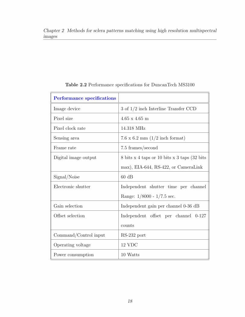
Table 2.2 Performance specifications for DuncanTech MS3100
Performance specifications
Image device 3 of 1/2 inch Interline Transfer CCD
Pixel size 4.65 x 4.65 m
Pixel clock rate 14.318 MHz
Sensing area 7.6 x 6.2 mm (1/2 inch format)
Frame rate 7.5 frames/second
Digital image output 8 bits x 4 taps or 10 bits x 3 taps (32 bits
max), EIA-644, RS-422, or CameraLink
Signal/Noise 60 dB
Electronic shutter Independent shutter time per channel
Range: 1/8000 - 1/7.5 sec.
Gain selection Independent gain per channel 0-36 dB
Offset selection Independent offset per channel 0-127
counts
Command/Control input RS-232 port
Operating voltage 12 VDC
Power consumption 10 Watts
18
Chapter 2 Methods for sclera patterns matching using high resolution multispectralimages
(a) (b) (c) (d)
Figure 2.4 (a) Right-eye-looking-left (R L). (b) Right-eye-looking-right(R R). (c) Left-eye-looking-left (L L). (d) Left-eye-looking-right (L R).
While the person is gazing to the left or to the right, Figure 2.4, the camera can be
easily manipulated to focus on the white of the eye. The light source (SL1-Filter,
StellarNet Inc.) illuminates the eye using a spectral range from 350 nm to 1700 nm,
and is projected onto the eye via an optic fiber guide with a ring light attached to
its end (HeiScope Annular Ring Light Guide). The amount of light is around 5.6 lux
measured with cal-LIGHT 400L lightmeter (Cooke Corporation) at the temple, near
the eye. Due to the reflective qualities of the eyeball, pointing a light source directly
at the subject’s eye creates a glare on the sclera. The issue is resolved by directing
the light source such that the incoming rays to the eyeball are approximately per-
pendicular to the pupil region. This is not always possible due to subtle movements
of the eyeball. Thus, glare is not always contained within the pupil region and may
overlap with the iris.
The multispectral camera generates images with a resolution of 1040 × 1392 × 3
pixels. The first 17 columns are removed due to artifacts. The final size of the images
is 1035 × 1373 × 3.
Collection 1
Videos of the right and left eye are captured from 103 subjects (Table 2.3), with
19

Chapter 2 Methods for sclera patterns matching using high resolution multispectralimages
each eye gazing to the right or to the left. Eight images per eye per gaze direc-
tion are selected from the video, based on a proper illumination, less specular
reflection and in focus images. The total number of images is 3280. For one
subject, only data from the right eye was collected due to medical issues. Work-
ing with images from the same video allows us to bypass some of the challenges
encountered by Crihalmeanu et al. [27] primarily due to viewing angle. The
process of frame selection ensures that there is no remarkable change in pose.
The camera is focused on the sclera region. Similarly the light is directed as
much as possible towards the sclera region with the specular reflection as much
as possible on the pupil. As a result in some images, mostly for left eye looking
right (L R) and right-eye-looking-left (R L) the iris is less illuminated in the
area close to the nose region.
Collection 2
Videos of the right and left eye are captured from 31 subjects (Table 2.3), with
each eye gazing to the right or to the left. To increase the intra-class variation,
the participant is asked to keep the head still and alternate the gaze direction
between looking at the ring of lights (left or right side direction) and looking
to the camera (frontal gaze direction) as illustrated in Figure 2.4. While gazing
to the left or to the right, the subject is asked to look at a mark located on
the ring of lights. Four images per eye per gaze direction are selected from the
video when looking left or looking right, after each change in gaze direction
from frontal to the side. The total number of images is 496. The multispectral
camera and the light are focused on the iris region. Due to the movement of
the eye and the selection process of the frames, the four ocular images/eye/gaze
have variations in viewing angle. Since the light is directed to the iris and due
to the curvature of the eyeball, some images have sclera region less illuminated
20
Chapter 2 Methods for sclera patterns matching using high resolution multispectralimages
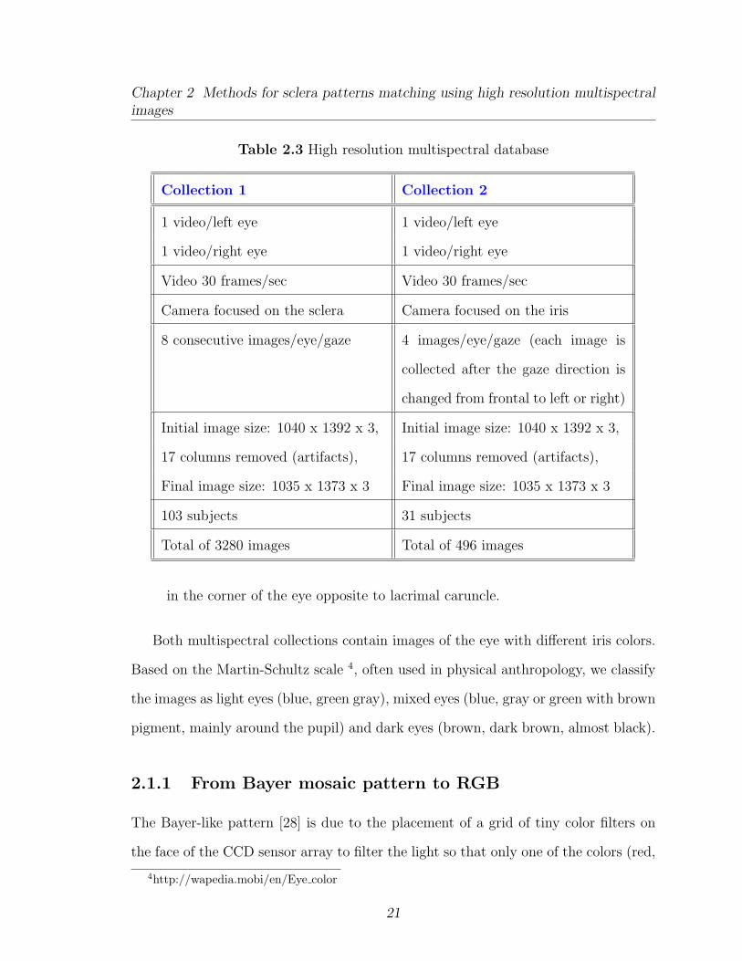
Table 2.3 High resolution multispectral database
Collection 1 Collection 2
1 video/left eye 1 video/left eye
1 video/right eye 1 video/right eye
Video 30 frames/sec Video 30 frames/sec
Camera focused on the sclera Camera focused on the iris
8 consecutive images/eye/gaze 4 images/eye/gaze (each image is
collected after the gaze direction is
changed from frontal to left or right)
Initial image size: 1040 x 1392 x 3, Initial image size: 1040 x 1392 x 3,
17 columns removed (artifacts), 17 columns removed (artifacts),
Final image size: 1035 x 1373 x 3 Final image size: 1035 x 1373 x 3
103 subjects 31 subjects
Total of 3280 images Total of 496 images
in the corner of the eye opposite to lacrimal caruncle.
Both multispectral collections contain images of the eye with different iris colors.
Based on the Martin-Schultz scale 4, often used in physical anthropology, we classify
the images as light eyes (blue, green gray), mixed eyes (blue, gray or green with brown
pigment, mainly around the pupil) and dark eyes (brown, dark brown, almost black).
2.1.1 From Bayer mosaic pattern to RGB
The Bayer-like pattern [28] is due to the placement of a grid of tiny color filters on
the face of the CCD sensor array to filter the light so that only one of the colors (red,
4http://wapedia.mobi/en/Eye color
21
Chapter 2 Methods for sclera patterns matching using high resolution multispectralimages
G4
G3
G1
G2
R1
R4
R3
R2 R G4
G3
G1
G2
B1
B4
B3
B2 B
(a) (b) (c)
Figure 2.5 Bayer pattern: a) Bayer pattern grid. b) Green component, redpixel interpolation. c) Green component, blue pixel interpolation (Adaptedfrom www.siliconimaging.com/RGB Bayer.htm).
blue or green) reaches any given pixel. Here, 25% of the pixels are assigned to blue,
25% to red and 50% to green. Blue and green components are obtained from the
Bayer mosaic pattern through interpolation 5. As illustrated in Figure 2.5, the value
of the green component on a red pixel is interpolated according to the strength of the
correlation on the vertical or horizontal direction of the neighboring red pixels:
G(R) =
(G1 +G3)/2 if | R1−R3 |<| R2−R4 |
(G2 +G4)/2 if | R1−R3 |>| R2−R4 |
(G1 +G2 +G3 +G4)/4 if | R1−R3 |=| R2−R4 |
(2.1)
The green component is interpolated on a blue pixel as follow:
G(B) =
(G1 +G3)/2 if | B1−B3 |<| B2−B4 |
(G2 +G4)/2 if | B1−B3 |>| B2−B4 |
(G1 +G2 +G3 +G4)/4 if | B1−B3 |=| B2−B4 |
(2.2)
The blue component values for green pixels are obtained in a similar way.
5RGB ”Bayer” Color and MicroLenses, www.siliconimaging.com/RGB Bayer.htm
22
Chapter 2 Methods for sclera patterns matching using high resolution multispectralimages
2.2 Image denoising
The red, green, blue and NIR components obtained from the CIR images are in
general noisy (Figure 2.6(a)(c)(e)(g)). The denoising algorithm employed is based
on a wavelet transformation. A double-density complex discrete wavelet transform
(DDCDWT) [29], which combines the characteristics and the properties of the double-
density discrete wavelet transform (DDDWT) [30] and the dual-tree discrete wavelet
transform (DTDWT) [1], is used. The transformation is based on two scaling func-
tions and four distinct wavelets such that one pair of wavelets form an approximate
Hilbert transform pair and the other pair of wavelets are offset from one other by one
half. It is implemented by applying four 2-D double density discrete wavelet trans-
forms in parallel to the input data with different filter sets for rows and columns,
yielding 32 oriented wavelets (Figure 2.7(a)) along one of six angles at ±15,±45,±75
degrees 6. The method is shift-invariant, possesses improved directional selectivity
and is based on FIR perfect reconstruction filter banks as illustrated in Figure 2.7(b).
For all scales and subbands, the magnitudes of the complex wavelet coefficients are
processed by soft thresholding that sets the coefficients with values less than a thresh-
old to zero and subtracts the threshold values from the non-zero coefficients. Original
and denoised red, green, blue and NIR images are presented in Figure 2.6. Visual
differences are not pronounced due to image rescaling. After denoising, all spectral
components (NIR, red, green and blue) are geometrically resized by a factor of 1/3
resulting in the final size of 310 × 411.
6http://taco.poly.edu/selesi/DoubleSoftware/index.html
23
Chapter 2 Methods for sclera patterns matching using high resolution multispectralimages
(a) (b) (c) (d)
(e) (f) (g) (h)
Figure 2.6 Denoising with Double Density Complex Discrete Wavelet Trans-form. a) Original NIR. b) Denoised NIR. c) Original red component. d)Denoised red component. e) Original green component. f) Denoised greencomponent. g) Original blue component. h) Denoised blue component. Vi-sual differences between original and denoised images are not pronounceddue to image rescaling.
2
2
2
H0
H1
H2
G0
G1
G2
2
2
2
H0
H1
H2
2
2
2
H0
H1
H2
2
2
2
2
2
2
G0
G1
G2
2
2
2
G0
G1
G2
(a) (b)
Figure 2.7 (a) Plot of Complex 2-D Double-Density Dual-Tree Wavelets.(b) Iterated filterbank for the Double-Density Complex Discrete WaveletTransform [1].
24
Chapter 2 Methods for sclera patterns matching using high resolution multispectralimages
2.3 Specular reflection detection and removal
Specular reflections have to be detected and removed as they can impact the sclera
segmentation process (described in Section 2.4). The light directed to the eyeball
generates specular reflection that has a ring-like shape, caused by the shape of the
source of illumination, and highlights, due to the moisture of the eye and the curved
shape of the eyeball. Both are detected and removed by a fast inpainting algorithm. In
some images, the ring-like shape may be an incomplete circle, ellipse, or an arbitrary
curved shape with a wide range of intensity values. It may be located partially
in the iris region, making its detection and removal more difficult especially since
the iris texture has to be preserved as much as possible. The specular reflections
are detected using different intensity threshold values for each component: 0.60 for
NIR, 0.50 for red and 0.80 for green. Only regions with less then 1000 pixels in
size are labeled as specular reflection, are morphologically dilated and inpainted. In
digital inpainting, the information from the boundary of the region to be inpainted
is propagated smoothly inside the region. The value to be inpainted at a pixel is
calculated using a PDE equation 7 in which partial derivatives are replaced by finite
differences between the pixel and its eight neighbors. Results are presented in Figure
2.8.
2.4 Sclera Region Segmentation
When the entire image of the eye is used for enhancing the conjunctival vasculature,
it is difficult to distinguish between the different types of lines that appear in it:
wrinkles, crows feet, eyelashes, blood vessels. Therefore, a good segmentation of the
sclera region that clearly exhibits the blood vessels is necessary. Even if the light is
7http://www.mathworks.com/matlabcentral/fileexchange/4551
25
Chapter 2 Methods for sclera patterns matching using high resolution multispectralimages
(a) (b)
Figure 2.8 Specular reflection removal: (a) Original image. (b) Originalimage with specular reflection removed.
directed to the pupil region to avoid specular reflections, the curved nature of the
eyeball presents a wide variety of intensity values across the sclera surface. Brighter
skin regions as a result of illumination, and occasionally the presence of mascara,
will make the segmentation of the sclera along the contour of the eyelid a challenging
process. The algorithm to segment the sclera region has three main steps as described
below.
2.4.1 Coarse sclera region segmentation: The sclera-eyelid
boundary
The method employed to segment the sclera region along the eyelid contour is inspired
by the work done in the processing of LandSat imagery (Land + Satellite) [31]. A set
of indices are used to segment the vegetation regions in aerial multispectral images.
Similarly, the index that we use for coarse sclera segmentation is based on the fact
that the skin has lesser water content than the sclera, and hence exhibits a higher
reflectance in NIR. Since water absorbs NIR light, the corresponding regions based
26
Chapter 2 Methods for sclera patterns matching using high resolution multispectralimages
(a) (b) (c)
Figure 2.9 Sclera region segmentation. The first row displays the originalimage, the second row displays the normalized sclera index: (a) Dark colorediris. (b) Light colored iris. (c) Mixed colored iris.
on this index appear dark in the image. The algorithm is as follows:
1. Compute an index called the normalized sclera index NSI(x, y) = NIR(x,y)−G(x,y)NIR(x,y)+G(x,y)
,
where NIR(x, y) and G(x, y) are the pixel intensities of the NIR and green
components, respectively, at pixel location (x, y). The difference NIR − G is
larger for pixels pertaining to the sclera region; it is then normalized to help
compensate for the uneven illumination. Figure 2.9 displays the normalized
sclera index for all three categories as specified by the Martin-Schultz scale:
light colored iris, dark colored iris and mixed colored iris.
2. Locate sclera by thresholding the NSI image with the threshold value η = 0.1.
Figure 2.10(a) displays the scatter plot between the NIR intensity values and
the corresponding green intensity values for all pixels in the image. The pixels
above the threshold (η = 0.1) represent the background region while the rest
represent the sclera region. Changing the value of η will modify the slope of the
boundary line between the pixels of the two segmented regions.
27
Chapter 2 Methods for sclera patterns matching using high resolution multispectralimages
−1 −0.5 0 0.5 10
2500
5000
7500
10000
12500
15000
0 0.2 0.4 0.6 0.8 10
0.2
0.4
0.6
0.8
1
Green level
NIR
leve
l
NIR vs. Green Scatter Plot
−1 −0.5 0 0.5 10
2000
4000
6000
8000
10000
12000
−1 −0.5 0 0.5 10
2000
4000
6000
8000
(a) (b) (c) (d)
Figure 2.10 Sclera region segmentation. The first row displays the resultsfor dark colored iris, the second row displays the results for light colored iris,and the third row displays the results for mixed colored iris: (a) NIR vs.greenintensity values. (b) Threshold applied to NSI. (c) Histogram of the NSI. (d)Sclera mask contour imposed on original composite image.
28

Chapter 2 Methods for sclera patterns matching using high resolution multispectralimages
The output of the thresholding operation is a binary image 8, Figure 2.10(b).
For each category in the Martin-Schultz classification, the largest connected
region in the binary image is composed of sclera region only; or the sclera and
the iris; or the sclera and a portion of the iris. For dark irides (brown and
dark brown), the sclera region excluding the iris is localized (Figure 2.10(d) the
first row, referred henceforth as IS). Thus, in this case, further segmentation
of the sclera and iris is not required. For light irides (blue, green, etc.), regions
pertaining to both the sclera and iris are segmented (Figure 2.10(d) the second
row, referred henceforth as IS). Here, further separation of the sclera and iris is
needed. For mixed irides (blue or green with brown around pupil), the region of
the sclera and the light colored portion of the iris are segmented as one region
(referred henceforth as IS). The dark portion of the iris (brown) is not included
(Figure 2.10(d) the third row). Here, further separation of the sclera and the
portion of the iris is needed. To finalize the segmentation of the sclera, i.e.,
to find the boundary between the sclera and the iris regardless of the color of
the iris, the pupil is detected. The convex hull of the segmented region IS and
the pupil region will contain the sclera, the pupil, and the iris or the portion of
the iris. This region is referred to as ISIP and is further processed. Since the
proposed algorithm does not deduce the color of the iris, it is applicable to all
images irrespective of the eye color. As seen in Figure 2.10(b), the location of
the pupil is also visible either as a dark region that does not overlap the sclera
region (in dark and mixed irides) or as a lighter disk within the sclera region
(in light irides). This information can be exploited only if the color of the iris
is known in advance. Therefore, in Section 2.4.2 we present an automatic way
8MathWorks, Image Processing Toolbox, Finding Vegetation in a Multispectral Image,
http://www.mathworks.com/products/image/demos.html
29

Chapter 2 Methods for sclera patterns matching using high resolution multispectralimages
of finding the pupil location regardless of the color of the iris.
2.4.2 Pupil region segmentation
The location of the pupil is needed to determine ISIP and to find the boundary
between the sclera and the iris regardless of the color of the eye. Hence, the accurate
determination of its boundary is not necessary. In NIR images, the pupil region is
characterized by very low intensity values and, by employing a simple threshold, the
pupil region is obtained. However, this isolates the eyelashes as well. In order to
isolate only the pupil, the following steps are undertaken:
1. Geometrically resize the NIR component by a factor of 1/3 and apply power-law
transformation [21] to its pixels: IPL = c ∗ IxI , where c = 1 is a constant, IPL is
the output image, II is the input NIR image and x = 0.7.
2. Threshold IPL with a value of 0.1. The resulting binary image, IBW , has the pupil
and eyelashes denoted by 1.
3. Find the contour of the convex hull of the sclera region as segmented in Section
2.4.1, ISCH , Figure 2.11 (b), (d).
4. Use Hough transform for line detection. Select and remove the highest peak cor-
responding to the longest line, Figure 2.11 (c), (d).
5. Fit an ellipse to the remaining sclera contour points, E(a, b, (x0, y0), θ), where a,
b, (x0, y0) and θ correspond to the length of the semi-major axes, length of
the semi-minor axes, the center of the ellipse, and its orientation, respectively
Figure 2.11 (e). Define an elliptical mask (to detect the pupil region) to extract
the pixels located within the ellipse.
30

Chapter 2 Methods for sclera patterns matching using high resolution multispectralimages
6. Impose the ellipse mask on the binary image IBW obtained in step 2. The result
is a binary image that will contain the pupil, and possibly eyelashes, as logical
1 pixels, IP .
7. Count the number of connected objects N in IP . If N > 1, through an iterative
process, decrease the ellipse’s semi-major and semi-minor axis (by 2%) and
construct new elliptical masks that when imposed on the binary image IBW will
render a smaller value for N. The connected object for N = 1 will correspond
to the location of the pupil.
while N > 1 do
a = a− 2100
× a,
b = b− 2100
× b,
EMASK = E(a, b, (x0, y0), θ)
IP = IBW ∩ EMASK
find N in IP
end while
8. Fit a new ellipse E to the dilated region corresponding to the location of the
pupil. Compute IP = IBW ∩ EMASK . Even if low intensity regions in the iris
are inadvertently selected, the pupil region has by far the largest area among
all connected objects.
9. Fit an ellipse to the pixels pertaining to the pupil region to find the pupil mask,
PMASK . Resize the pupil mask to the original NIR image size Figure 2.11 (f).
The procedure described above is applied to all the images regardless of the color
of the iris. For 15 images, the algorithm failed to correctly segment the pupil.
31
Chapter 2 Methods for sclera patterns matching using high resolution multispectralimages
θ
ρ
−50 0 50
−1000
0
1000
Highest peak
θ
ρ
−50 0 50
−1000
0
1000
Highest peak
(a) (b) (c)
(d) (e) (f)
Figure 2.11 Pupil region segmentation. The first row displays the results fordark colored iris, the second row displays the results for light colored iris: (a)Original image. (b) Convex hull of the sclera region. (c) Hough transformand the highest peak. (d) Sclera region contour and the longest line. (e)The ellipse fitted to the sclera contour. (f) Output of the pupil segmentationalgorithm.
32
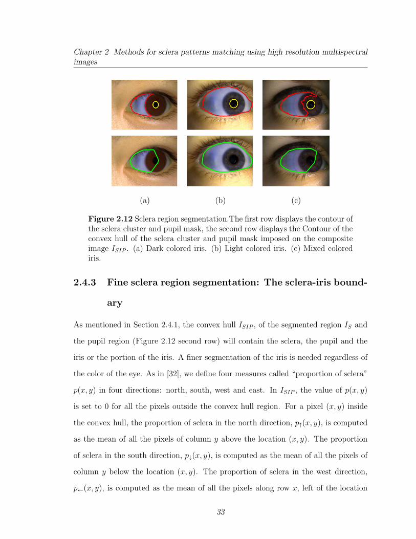
Chapter 2 Methods for sclera patterns matching using high resolution multispectralimages
(a) (b) (c)
Figure 2.12 Sclera region segmentation.The first row displays the contour ofthe sclera cluster and pupil mask, the second row displays the Contour of theconvex hull of the sclera cluster and pupil mask imposed on the compositeimage ISIP . (a) Dark colored iris. (b) Light colored iris. (c) Mixed colorediris.
2.4.3 Fine sclera region segmentation: The sclera-iris bound-
ary
As mentioned in Section 2.4.1, the convex hull ISIP , of the segmented region IS and
the pupil region (Figure 2.12 second row) will contain the sclera, the pupil and the
iris or the portion of the iris. A finer segmentation of the iris is needed regardless of
the color of the eye. As in [32], we define four measures called “proportion of sclera”
p(x, y) in four directions: north, south, west and east. In ISIP , the value of p(x, y)
is set to 0 for all the pixels outside the convex hull region. For a pixel (x, y) inside
the convex hull, the proportion of sclera in the north direction, p↑(x, y), is computed
as the mean of all the pixels of column y above the location (x, y). The proportion
of sclera in the south direction, p↓(x, y), is computed as the mean of all the pixels of
column y below the location (x, y). The proportion of sclera in the west direction,
p←(x, y), is computed as the mean of all the pixels along row x, left of the location
33
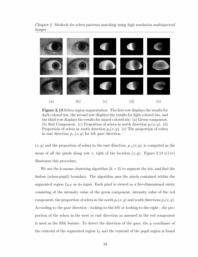
Chapter 2 Methods for sclera patterns matching using high resolution multispectralimages
(a) (b) (c) (d) (e)
Figure 2.13 Sclera region segmentation. The first row displays the results fordark colored iris, the second row displays the results for light colored iris, andthe third row displays the results for mixed colored iris: (a) Green component.(b) Red Component. (c) Proportion of sclera in north direction p↑(x, y). (d)Proportion of sclera in south direction p↓(x, y). (e) The proportion of sclerain east direction p←(x, y) for left gaze direction.
(x, y) and the proportion of sclera in the east direction, p→(x, y), is computed as the
mean of all the pixels along row x, right of the location (x, y). Figure 2.13 (c)-(e)
illustrates this procedure.
We use the k-means clustering algorithm (k = 2) to segment the iris, and find the
limbus (sclera-pupil) boundary. The algorithm uses the pixels contained within the
segmented region ISIP as its input. Each pixel is viewed as a five-dimensional entity
consisting of the intensity value of the green component, intensity value of the red
component, the proportion of sclera in the north p↑(x, y) and south directions p↓(x, y).
According to the gaze direction - looking-to-the-left or looking-to-the-right - the pro-
portion of the sclera in the west or east direction as assessed in the red component
is used as the fifth feature. To detect the direction of the gaze, the y coordinate of
the centroid of the segmented region IS and the centroid of the pupil region is found
34

Chapter 2 Methods for sclera patterns matching using high resolution multispectralimages
and compared. For the left gaze direction ypupil > ysclera and proportion of sclera in
the east direction is used; for the right gaze direction ypupil < ysclera and the propor-
tion of sclera in the west direction is used. Euclidean distances between the origin
of the coordinate system and the centroid of each cluster are computed in order to
determine the label of the two clusters (the label can be ‘sclera’ or ‘iris’). The largest
distance is associated with the sclera cluster; this is the white region in Figure 2.14
first row. The smallest distance is associated with the iris cluster; this is the black
region in Figure 2.14 first row. Two binary images, a mask for the sclera region and
a mask for the iris region represent the output. On examining the two binary masks,
we observe that in some images, the k-means algorithm erroneously labels portion of
the sclera as being the iris (mainly the corners of the sclera that are less illuminated
and have lower intensity values). To address this issue, if the iris mask has more than
one connected region, the region in the iris mask that overlaps with the pupil mask
is assumed to be the iris region, and is subtracted from the convex hull ISIP .
The algorithm failed to segment the sclera region properly for a total number of
151 images. This is due to improper illumination and plenty of mascara (Figure 2.15)
present in some images. The pupil segmentation algorithm finds the convex hull of
the sclera region. This method creates straight lines along the contour of the sclera.
For dark colored irides and mix colored irides, the longest induced line that is to be
removed using Hough transform (Section 2.4.2) connects the highest point with the
lowest point on the curved boundary of the iris and sclera (Figure 2.16 (a), the red
line). It may happen that the longest line induced by the convex hull is not the proper
one, but one that is located along the sclera contour (Figure 2.16 (b)). As a result,
after removal of the line with Hough transform, the fitted ellipse to the contour of
the sclera will no longer generate the elliptical mask needed.
35
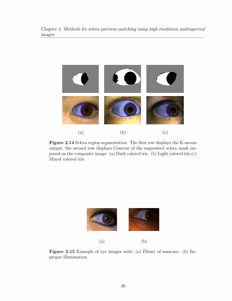
Chapter 2 Methods for sclera patterns matching using high resolution multispectralimages
(a) (b) (c)
Figure 2.14 Sclera region segmentation. The first row displays the K-meansoutput, the second row displays Contour of the segmented sclera mask im-posed on the composite image: (a) Dark colored iris. (b) Light colored iris.(c)Mixed colored iris.
(a) (b)
Figure 2.15 Example of eye images with: (a) Plenty of mascara. (b) Im-proper illumination.
36
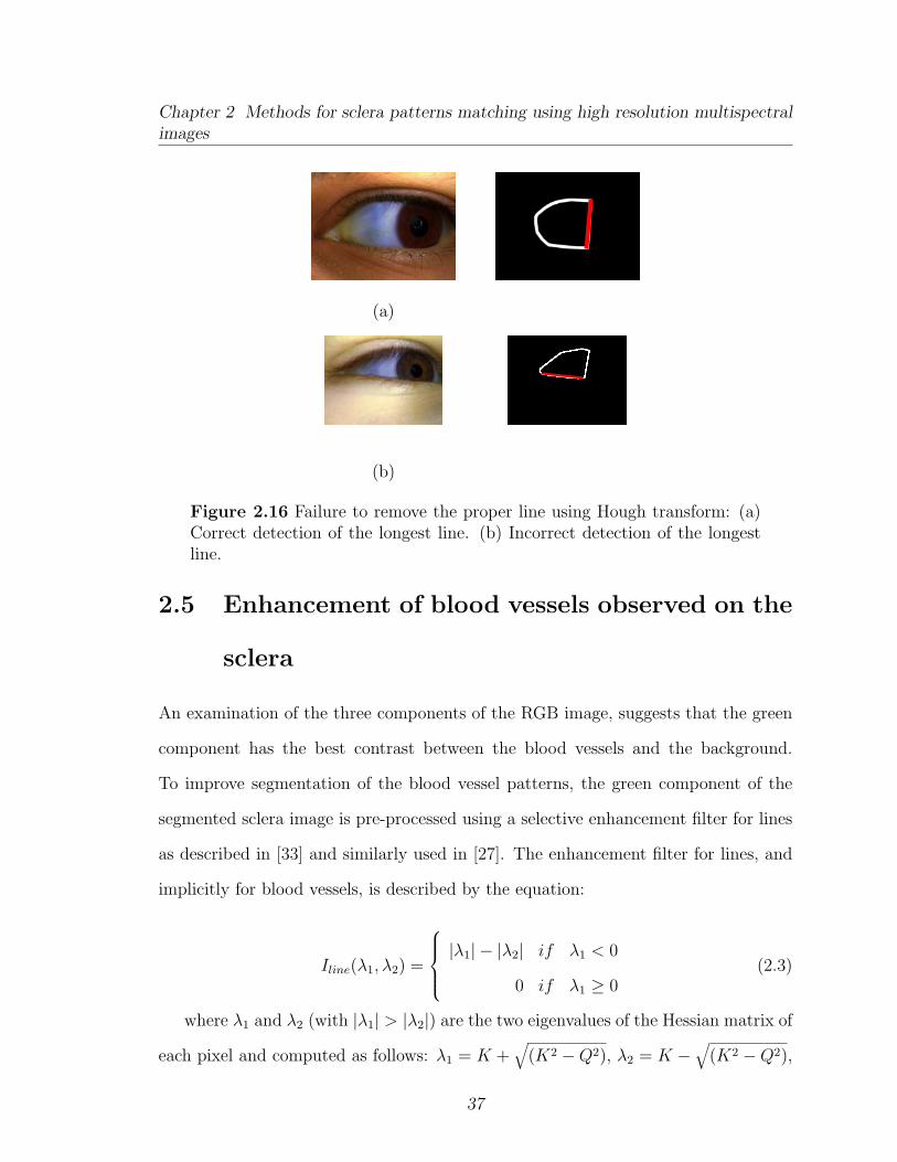
Chapter 2 Methods for sclera patterns matching using high resolution multispectralimages
(a)
(b)
Figure 2.16 Failure to remove the proper line using Hough transform: (a)Correct detection of the longest line. (b) Incorrect detection of the longestline.
2.5 Enhancement of blood vessels observed on the
sclera
An examination of the three components of the RGB image, suggests that the green
component has the best contrast between the blood vessels and the background.
To improve segmentation of the blood vessel patterns, the green component of the
segmented sclera image is pre-processed using a selective enhancement filter for lines
as described in [33] and similarly used in [27]. The enhancement filter for lines, and
implicitly for blood vessels, is described by the equation:
Iline(λ1, λ2) =
|λ1| − |λ2| if λ1 < 0
0 if λ1 ≥ 0(2.3)
where λ1 and λ2 (with |λ1| > |λ2|) are the two eigenvalues of the Hessian matrix of
each pixel and computed as follows: λ1 = K +√(K2 −Q2), λ2 = K −
√(K2 −Q2),
37
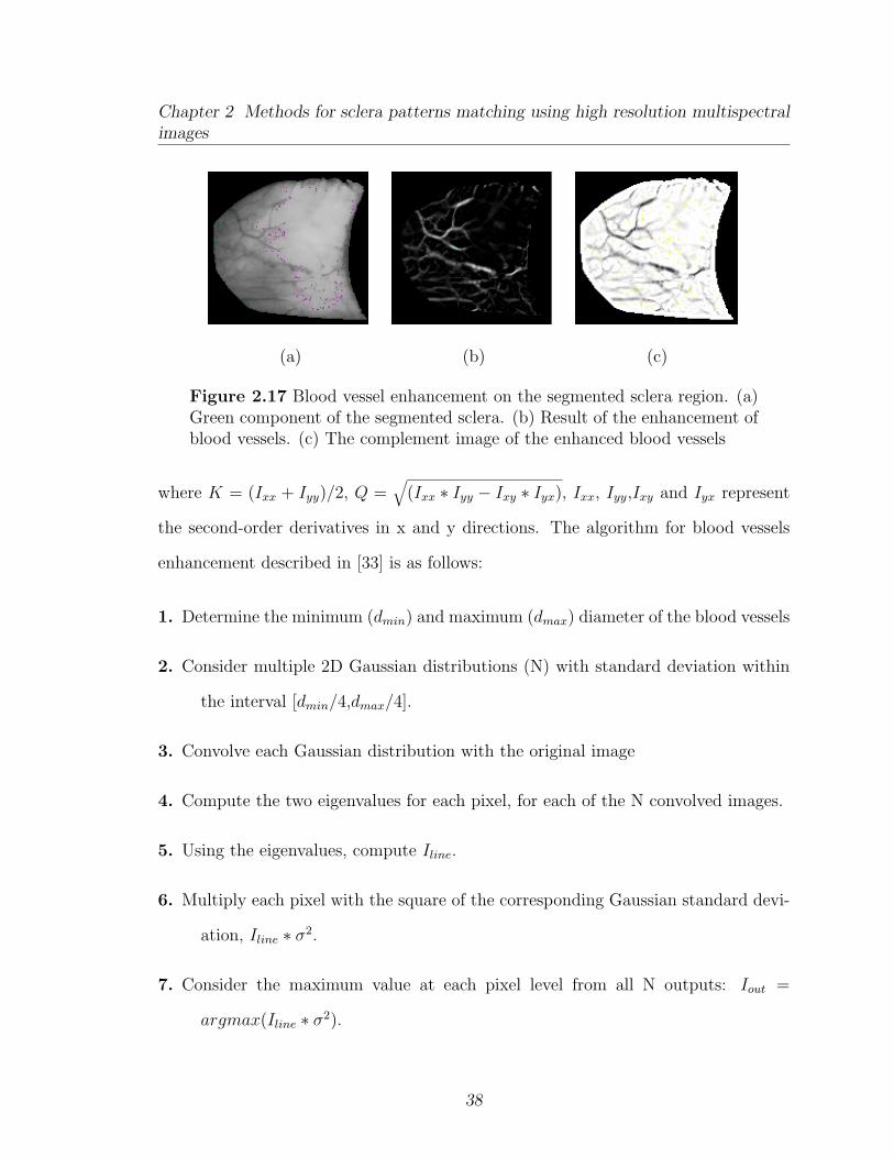
Chapter 2 Methods for sclera patterns matching using high resolution multispectralimages
(a) (b) (c)
Figure 2.17 Blood vessel enhancement on the segmented sclera region. (a)Green component of the segmented sclera. (b) Result of the enhancement ofblood vessels. (c) The complement image of the enhanced blood vessels
where K = (Ixx + Iyy)/2, Q =√(Ixx ∗ Iyy − Ixy ∗ Iyx), Ixx, Iyy,Ixy and Iyx represent
the second-order derivatives in x and y directions. The algorithm for blood vessels
enhancement described in [33] is as follows:
1. Determine the minimum (dmin) and maximum (dmax) diameter of the blood vessels
2. Consider multiple 2D Gaussian distributions (N) with standard deviation within
the interval [dmin/4,dmax/4].
3. Convolve each Gaussian distribution with the original image
4. Compute the two eigenvalues for each pixel, for each of the N convolved images.
5. Using the eigenvalues, compute Iline.
6. Multiply each pixel with the square of the corresponding Gaussian standard devi-
ation, Iline ∗ σ2.
7. Consider the maximum value at each pixel level from all N outputs: Iout =
argmax(Iline ∗ σ2).
38

Chapter 2 Methods for sclera patterns matching using high resolution multispectralimages
2.6 Image registration
In this method, the two images to be compared are first registered using an im-
age alignment scheme, and a direct correlation between corresponding pixels is then
used to determine their similarity. Image registration is the process of finding a
transformation that aligns one image with another. The regions of the sclera in
the two images that are to be registered are cropped, and the images are padded
to the same size. The image with the smaller height is padded up and down with
an equal number of rows. If the gaze direction of the eye is to the left, the im-
age with the smaller width is padded to the right. If the gaze direction of the eye
is to the right, the image with the smaller width is padded to the left. To detect
the direction of the gaze, the y coordinate of the centroid of the sclera region and
the centroid of the pupil region is found and compared. This process results in a
better overlap of the two sclera regions. The registration method used here, de-
scribed in [34], models a local affine and a global smooth transformation. It also
accounts for contrast and brightness variations between the two images that are to be
registered. The registration between two images, the source I(x, y, t) and the target
I(x, y, t−1), is modeled by the transformation m = (m1,m2,m3,m4,m5,m6,m7,m8):
m7I(x, y, t)+m8 = I(m1x+m2y+m5,m3x+m4y+m6, t−1), wherem1,m2,m3, and m4
are the linear affine parameters, m5,m6 are the translation parameters, and m7,m8
are the contrast and brightness parameters. A multi-scale approach is employed by
using a Gaussian pyramid to downsample the images to be registered. From a coarse-
to-fine level, the transformation m is determined globally at each level, and then
locally, and the estimated parameters are used to warp the source image. Using the
linear affine parameters m1,m2,m3, and m4, and the translation parameters m5,m6,
the sclera mask of the source image is also registered. Figure 2.18 shows results for
39
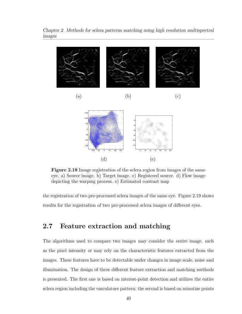
Chapter 2 Methods for sclera patterns matching using high resolution multispectralimages
(a) (b) (c)
−100 −50 0 50 100 150
−150
−100
−50
0
50
100
150
20 40 60 80 100 120 140
20
40
60
80
100
120
(d) (e)
Figure 2.18 Image registration of the sclera region from images of the sameeye. a) Source image. b) Target image. c) Registered source. d) Flow imagedepicting the warping process. e) Estimated contrast map
the registration of two pre-processed sclera images of the same eye. Figure 2.19 shows
results for the registration of two pre-processed sclera images of different eyes.
2.7 Feature extraction and matching
The algorithms used to compare two images may consider the entire image, such
as the pixel intensity or may rely on the characteristic features extracted from the
images. These features have to be detectable under changes in image scale, noise and
illumination. The design of three different feature extraction and matching methods
is presented. The first one is based on interest-point detection and utilizes the entire
sclera region including the vasculature pattern; the second is based on minutiae points
40
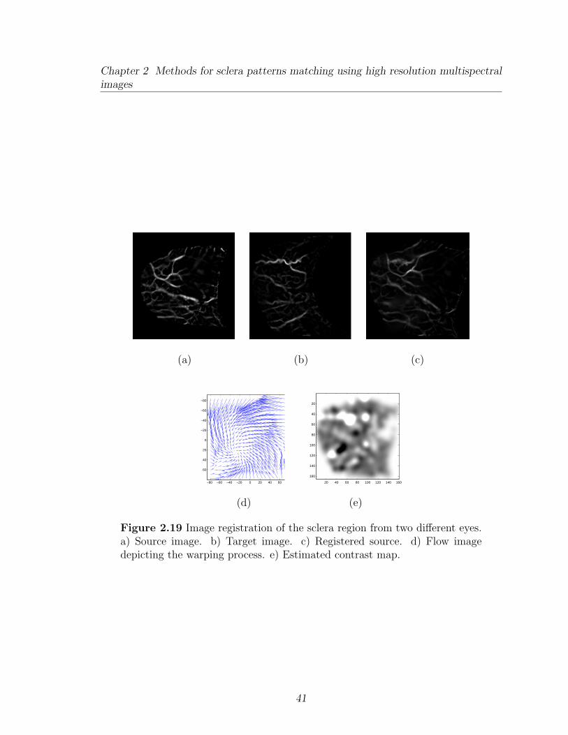
Chapter 2 Methods for sclera patterns matching using high resolution multispectralimages
(a) (b) (c)
−80 −60 −40 −20 0 20 40 60
−80
−60
−40
−20
0
20
40
60
20 40 60 80 100 120 140 160
20
40
60
80
100
120
140
160
(d) (e)
Figure 2.19 Image registration of the sclera region from two different eyes.a) Source image. b) Target image. c) Registered source. d) Flow imagedepicting the warping process. e) Estimated contrast map.
41
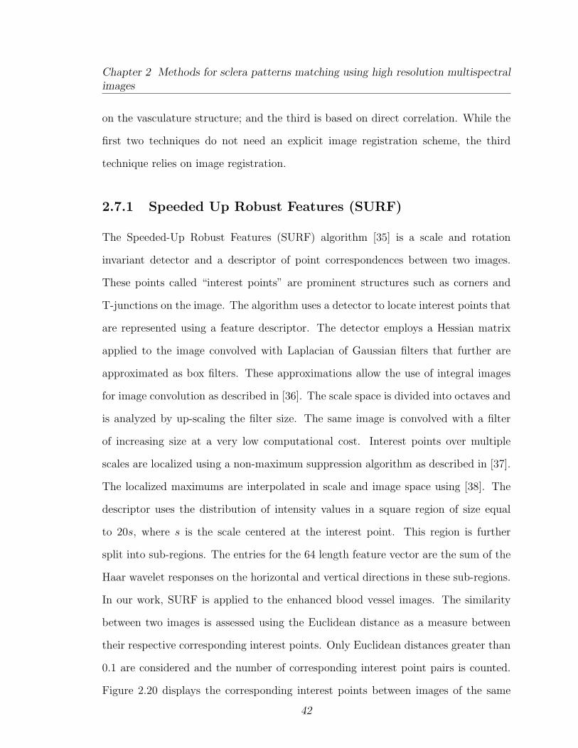
Chapter 2 Methods for sclera patterns matching using high resolution multispectralimages
on the vasculature structure; and the third is based on direct correlation. While the
first two techniques do not need an explicit image registration scheme, the third
technique relies on image registration.
2.7.1 Speeded Up Robust Features (SURF)
The Speeded-Up Robust Features (SURF) algorithm [35] is a scale and rotation
invariant detector and a descriptor of point correspondences between two images.
These points called “interest points” are prominent structures such as corners and
T-junctions on the image. The algorithm uses a detector to locate interest points that
are represented using a feature descriptor. The detector employs a Hessian matrix
applied to the image convolved with Laplacian of Gaussian filters that further are
approximated as box filters. These approximations allow the use of integral images
for image convolution as described in [36]. The scale space is divided into octaves and
is analyzed by up-scaling the filter size. The same image is convolved with a filter
of increasing size at a very low computational cost. Interest points over multiple
scales are localized using a non-maximum suppression algorithm as described in [37].
The localized maximums are interpolated in scale and image space using [38]. The
descriptor uses the distribution of intensity values in a square region of size equal
to 20s, where s is the scale centered at the interest point. This region is further
split into sub-regions. The entries for the 64 length feature vector are the sum of the
Haar wavelet responses on the horizontal and vertical directions in these sub-regions.
In our work, SURF is applied to the enhanced blood vessel images. The similarity
between two images is assessed using the Euclidean distance as a measure between
their respective corresponding interest points. Only Euclidean distances greater than
0.1 are considered and the number of corresponding interest point pairs is counted.
Figure 2.20 displays the corresponding interest points between images of the same
42
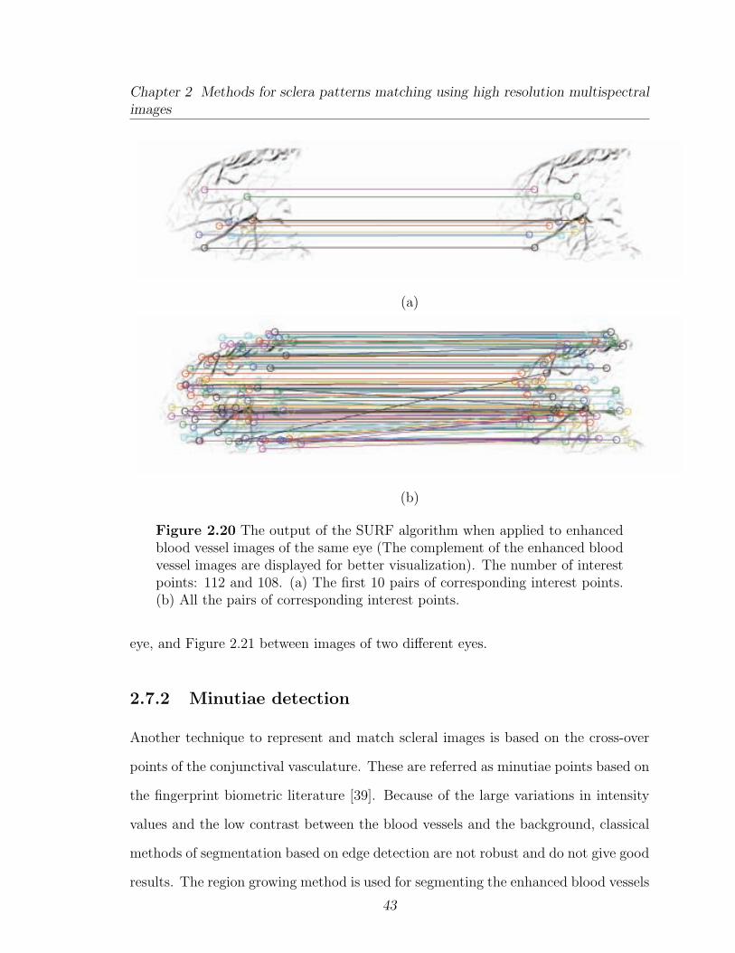
Chapter 2 Methods for sclera patterns matching using high resolution multispectralimages
(a)
(b)
Figure 2.20 The output of the SURF algorithm when applied to enhancedblood vessel images of the same eye (The complement of the enhanced bloodvessel images are displayed for better visualization). The number of interestpoints: 112 and 108. (a) The first 10 pairs of corresponding interest points.(b) All the pairs of corresponding interest points.
eye, and Figure 2.21 between images of two different eyes.
2.7.2 Minutiae detection
Another technique to represent and match scleral images is based on the cross-over
points of the conjunctival vasculature. These are referred as minutiae points based on
the fingerprint biometric literature [39]. Because of the large variations in intensity
values and the low contrast between the blood vessels and the background, classical
methods of segmentation based on edge detection are not robust and do not give good
results. The region growing method is used for segmenting the enhanced blood vessels
43
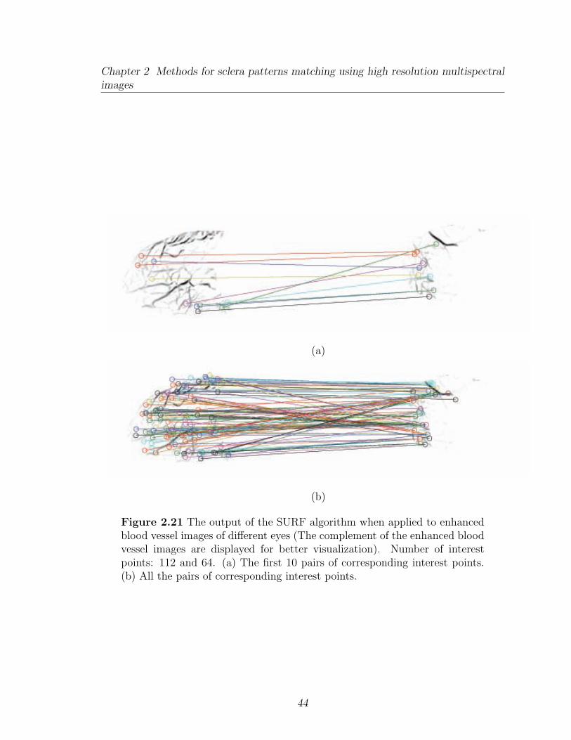
Chapter 2 Methods for sclera patterns matching using high resolution multispectralimages
(a)
(b)
Figure 2.21 The output of the SURF algorithm when applied to enhancedblood vessel images of different eyes (The complement of the enhanced bloodvessel images are displayed for better visualization). Number of interestpoints: 112 and 64. (a) The first 10 pairs of corresponding interest points.(b) All the pairs of corresponding interest points.
44
Chapter 2 Methods for sclera patterns matching using high resolution multispectralimages
(a) (b)
Figure 2.22 The centerline of the segmented blood vessels imposed on thegreen component of two images.
based on the algorithm described in [40]. The labeling of each pixel as pertaining to
the conjunctival vasculature or background, is based on the information provided by
the intensity value and the magnitude of the gradient of the pre-processed image.
The result of conjunctival vasculature segmentation using region growing is a binary
image, that is subjected to morphological operations, mainly a thinning procedure
through which the blood vessel thickness is reduced to one pixel (Figure 2.23 (b)).
The minutiae points, in this work, correspond to the bifurcations of the center-
line of the blood vessels (Figure 2.23 (c). Each blood vessel ramification has to
be as least 4 pixels in length. A point matching algorithm is used to compare the
points extracted from two images where each point is characterized as a (x, y) lo-
cation. The matching algorithm consists of finding an alignment between the two
sets of points that will result in the maximum overlap of minutiae pairs from the
two images. For two minutiae sets, A = {a1, a2, a3, ...am}, ai = (xi, yi), i = 1..m
and B = {b1, b2, b3, ...bn}, bj = (xj, yj), j = 1..n, where m and n are the number of
minutiae in A and B, minutiae ai is said to be in correspondence with a minutiae
bj if the Euclidean distance (E) between them is smaller than a given tolerance t ,
i.e., E(ai, bj) =√((xj − xi)2 + (yj − yi)2) ≤ t. The match score is computed as the
square of the number of corresponding minutiae points divided by the product mn.
The algorithm failed to detect minutiae points on 28 images. This is due to the de-
45

Chapter 2 Methods for sclera patterns matching using high resolution multispectralimages
(a) (b) (c)
Figure 2.23Detection of minutiae points. (a) Enhanced blood vessels image.(b) Centerline of the detected blood vessels. (c) Minutiae points: bifurcations(red) and endings (green).
(a) (b)
Figure 2.24 Failure to detect minutiae points. (a) Enhanced blood vesselsimage. (b) The detected vasculature without ramifications and intersections(Morphological operations such as dilation is applied to the blood vessels fora better visualization).
tection of blood vessels without ramifications and blood vessels that do not intersect
(Figure 2.24).
2.7.3 Direct correlation
Different measures are used to compare two registered sclera images. These measures
provide a quantitative score that describes the degree of similarity or conversely the
degree of error/distortion between two images. To generate genuine scores, the mea-
sure is computed between pairs of images pertaining to the same subject; to generate
impostor scores, the measure is computed between the first image (from the set of
46
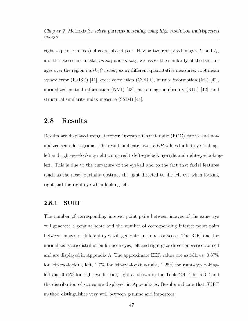
Chapter 2 Methods for sclera patterns matching using high resolution multispectralimages
eight sequence images) of each subject pair. Having two registered images I1 and I2,
and the two sclera masks, mask1 and mask2, we assess the similarity of the two im-
ages over the region mask1∩mask2 using different quantitative measures: root mean
square error (RMSE) [41], cross-correlation (CORR), mutual information (MI) [42],
normalized mutual information (NMI) [43], ratio-image uniformity (RIU) [42], and
structural similarity index measure (SSIM) [44].
2.8 Results
Results are displayed using Receiver Operator Charateristic (ROC) curves and nor-
malized score histograms. The results indicate lower EER values for left-eye-looking-
left and right-eye-looking-right compared to left-eye-looking-right and right-eye-looking-
left. This is due to the curvature of the eyeball and to the fact that facial features
(such as the nose) partially obstruct the light directed to the left eye when looking
right and the right eye when looking left.
2.8.1 SURF
The number of corresponding interest point pairs between images of the same eye
will generate a genuine score and the number of corresponding interest point pairs
between images of different eyes will generate an impostor score. The ROC and the
normalized score distribution for both eyes, left and right gaze direction were obtained
and are displayed in Appendix A. The approximate EER values are as follows: 0.37%
for left-eye-looking left, 1.7% for left-eye-looking-right, 1.25% for right-eye-looking-
left and 0.75% for right-eye-looking-right as shown in the Table 2.4. The ROC and
the distribution of scores are displayed in Appendix A. Results indicate that SURF
method distinguishes very well between genuine and impostors.
47
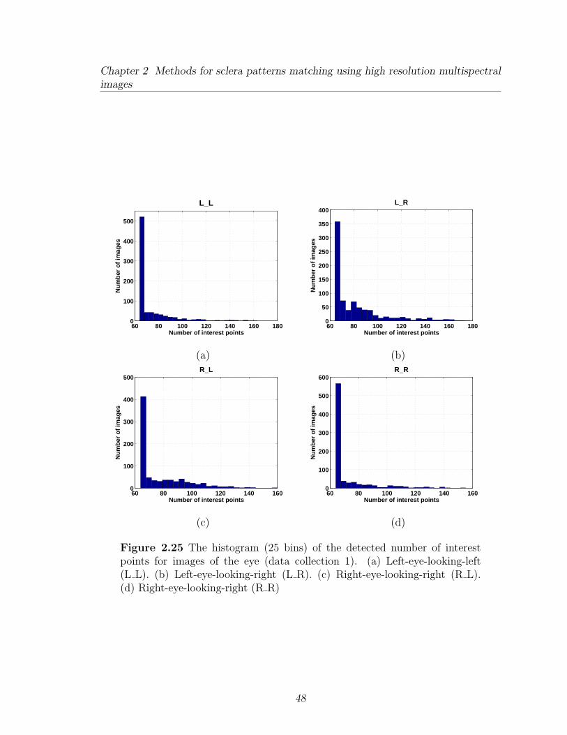
Chapter 2 Methods for sclera patterns matching using high resolution multispectralimages
60 80 100 120 140 160 1800
100
200
300
400
500
L_L
Number of interest points
Nu
mb
er o
f im
ages
60 80 100 120 140 160 1800
50
100
150
200
250
300
350
400L_R
Number of interest points
Nu
mb
er o
f im
ages
(a) (b)
60 80 100 120 140 1600
100
200
300
400
500R_L
Number of interest points
Nu
mb
er o
f im
ages
60 80 100 120 140 1600
100
200
300
400
500
600
Number of interest points
Nu
mb
er o
f im
ages
R_R
(c) (d)
Figure 2.25 The histogram (25 bins) of the detected number of interestpoints for images of the eye (data collection 1). (a) Left-eye-looking-left(L L). (b) Left-eye-looking-right (L R). (c) Right-eye-looking-right (R L).(d) Right-eye-looking-right (R R)
48
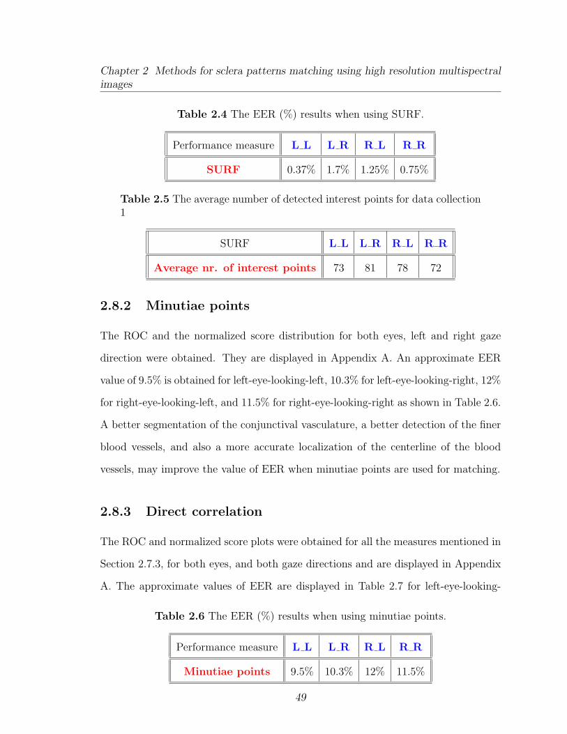
Chapter 2 Methods for sclera patterns matching using high resolution multispectralimages
Table 2.4 The EER (%) results when using SURF.
Performance measure L L L R R L R R
SURF 0.37% 1.7% 1.25% 0.75%
Table 2.5 The average number of detected interest points for data collection1
SURF L L L R R L R R
Average nr. of interest points 73 81 78 72
2.8.2 Minutiae points
The ROC and the normalized score distribution for both eyes, left and right gaze
direction were obtained. They are displayed in Appendix A. An approximate EER
value of 9.5% is obtained for left-eye-looking-left, 10.3% for left-eye-looking-right, 12%
for right-eye-looking-left, and 11.5% for right-eye-looking-right as shown in Table 2.6.
A better segmentation of the conjunctival vasculature, a better detection of the finer
blood vessels, and also a more accurate localization of the centerline of the blood
vessels, may improve the value of EER when minutiae points are used for matching.
2.8.3 Direct correlation
The ROC and normalized score plots were obtained for all the measures mentioned in
Section 2.7.3, for both eyes, and both gaze directions and are displayed in Appendix
A. The approximate values of EER are displayed in Table 2.7 for left-eye-looking-
Table 2.6 The EER (%) results when using minutiae points.
Performance measure L L L R R L R R
Minutiae points 9.5% 10.3% 12% 11.5%
49
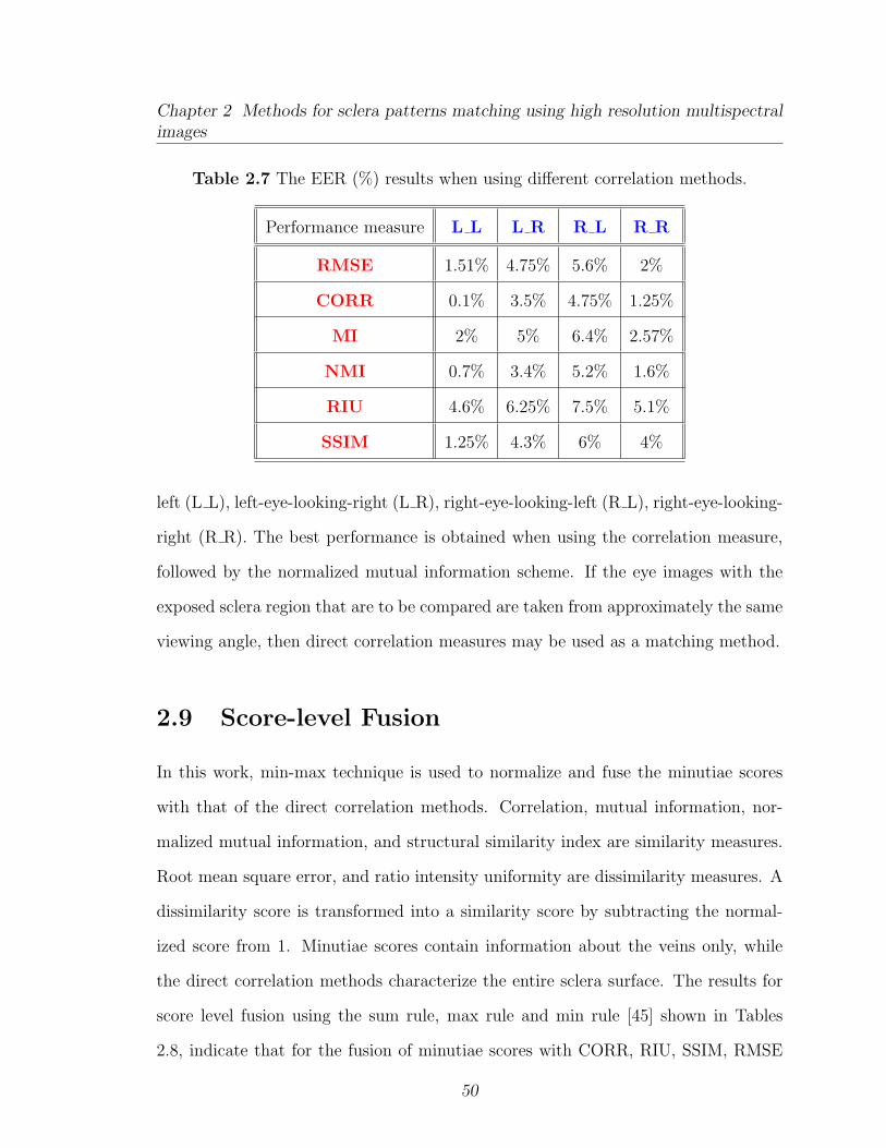
Chapter 2 Methods for sclera patterns matching using high resolution multispectralimages
Table 2.7 The EER (%) results when using different correlation methods.
Performance measure L L L R R L R R
RMSE 1.51% 4.75% 5.6% 2%
CORR 0.1% 3.5% 4.75% 1.25%
MI 2% 5% 6.4% 2.57%
NMI 0.7% 3.4% 5.2% 1.6%
RIU 4.6% 6.25% 7.5% 5.1%
SSIM 1.25% 4.3% 6% 4%
left (L L), left-eye-looking-right (L R), right-eye-looking-left (R L), right-eye-looking-
right (R R). The best performance is obtained when using the correlation measure,
followed by the normalized mutual information scheme. If the eye images with the
exposed sclera region that are to be compared are taken from approximately the same
viewing angle, then direct correlation measures may be used as a matching method.
2.9 Score-level Fusion
In this work, min-max technique is used to normalize and fuse the minutiae scores
with that of the direct correlation methods. Correlation, mutual information, nor-
malized mutual information, and structural similarity index are similarity measures.
Root mean square error, and ratio intensity uniformity are dissimilarity measures. A
dissimilarity score is transformed into a similarity score by subtracting the normal-
ized score from 1. Minutiae scores contain information about the veins only, while
the direct correlation methods characterize the entire sclera surface. The results for
score level fusion using the sum rule, max rule and min rule [45] shown in Tables
2.8, indicate that for the fusion of minutiae scores with CORR, RIU, SSIM, RMSE
50
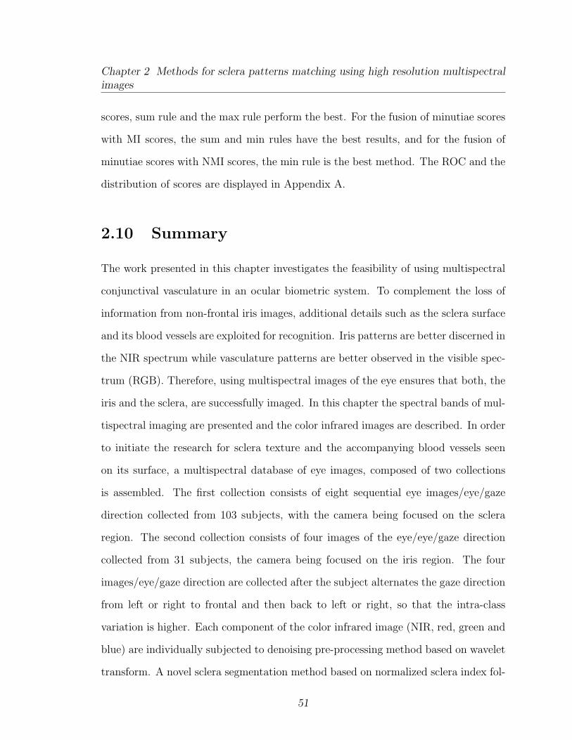
Chapter 2 Methods for sclera patterns matching using high resolution multispectralimages
scores, sum rule and the max rule perform the best. For the fusion of minutiae scores
with MI scores, the sum and min rules have the best results, and for the fusion of
minutiae scores with NMI scores, the min rule is the best method. The ROC and the
distribution of scores are displayed in Appendix A.
2.10 Summary
The work presented in this chapter investigates the feasibility of using multispectral
conjunctival vasculature in an ocular biometric system. To complement the loss of
information from non-frontal iris images, additional details such as the sclera surface
and its blood vessels are exploited for recognition. Iris patterns are better discerned in
the NIR spectrum while vasculature patterns are better observed in the visible spec-
trum (RGB). Therefore, using multispectral images of the eye ensures that both, the
iris and the sclera, are successfully imaged. In this chapter the spectral bands of mul-
tispectral imaging are presented and the color infrared images are described. In order
to initiate the research for sclera texture and the accompanying blood vessels seen
on its surface, a multispectral database of eye images, composed of two collections
is assembled. The first collection consists of eight sequential eye images/eye/gaze
direction collected from 103 subjects, with the camera being focused on the sclera
region. The second collection consists of four images of the eye/eye/gaze direction
collected from 31 subjects, the camera being focused on the iris region. The four
images/eye/gaze direction are collected after the subject alternates the gaze direction
from left or right to frontal and then back to left or right, so that the intra-class
variation is higher. Each component of the color infrared image (NIR, red, green and
blue) are individually subjected to denoising pre-processing method based on wavelet
transform. A novel sclera segmentation method based on normalized sclera index fol-
51
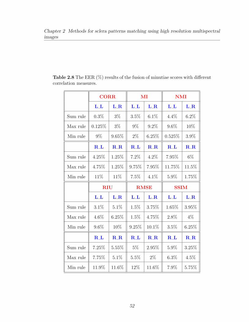
Chapter 2 Methods for sclera patterns matching using high resolution multispectralimages
Table 2.8 The EER (%) results of the fusion of minutiae scores with differentcorrelation measures.
CORR MI NMI
L L L R L L L R L L L R
Sum rule 0.3% 3% 3.5% 6.1% 4.4% 6.2%
Max rule 0.125% 3% 9% 9.2% 9.6% 10%
Min rule 9% 9.65% 2% 6.25% 0.525% 3.9%
R L R R R L R R R L R R
Sum rule 4.25% 1.25% 7.2% 4.2% 7.95% 6%
Max rule 4.75% 1.25% 9.75% 7.95% 11.75% 11.5%
Min rule 11% 11% 7.5% 4.1% 5.9% 1.75%
RIU RMSE SSIM
L L L R L L L R L L L R
Sum rule 3.1% 5.1% 1.5% 3.75% 1.65% 3.95%
Max rule 4.6% 6.25% 1.5% 4.75% 2.8% 4%
Min rule 9.6% 10% 9.25% 10.1% 3.5% 6.25%
R L R R R L R R R L R R
Sum rule 7.25% 5.55% 5% 2.95% 5.9% 3.25%
Max rule 7.75% 5.1% 5.5% 2% 6.3% 4.5%
Min rule 11.9% 11.6% 12% 11.6% 7.9% 5.75%
52
Chapter 2 Methods for sclera patterns matching using high resolution multispectralimages
lowed by thresholding is applied to the first collection of the multispectral database.
The pupil region segmentation based on power law transformation and multiple fitted
ellipses is described. Processing techniques such as vasculature enhancement using
a selective enhancement filter for lines, and implicitly for blood vessels is presented.
Further, the images of the eye are registered with a global smooth and a local affine
transformation based on intensity values. The design of three different feature ex-
traction and matching methods is presented. The first one is based on interest-point
detection and utilizes the entire sclera region including the vasculature pattern; the
second is based on minutiae points on the vasculature structure; and the third is based
on direct correlation. While the first two techniques do not need an explicit image
registration scheme, the third technique relies on image registration. The results
demonstrate the validity of using the sclera surface and the conjunctival vasculature
for recognition and support further investigation in this area of research.
53
Chapter 3
Fusion of iris patterns with scleral
patterns
Iris recognition performance is greatly and negatively influenced by the occlusions,
the lighting conditions and the direction of the gaze of the eye with respect to the
acquisition device. The use of the sclera as a biometric may be significant in the
context of iris recognition, when changes in the gaze angle of the eye can result in
non-frontal iris images that cannot be easily recognized. The more the gaze direction
deviates from the frontal pose, the more information from the iris texture is lost and
the more information from the sclera region is gained. The combined sclera and the
iris texture may be used in non-cooperative recognition when the probability of non-
ideal iris occurrence is greatly increased. By utilizing the texture of the sclera along
with the vascular patterns evident on it, the performance of an iris recognition system
can potentially be improved. The block diagram of the proposed system is shown in
Figure 3.1. In this approach the multispectral collection 1 is used. Image acquisition
and image denoising were presented in Chapter 2.
54
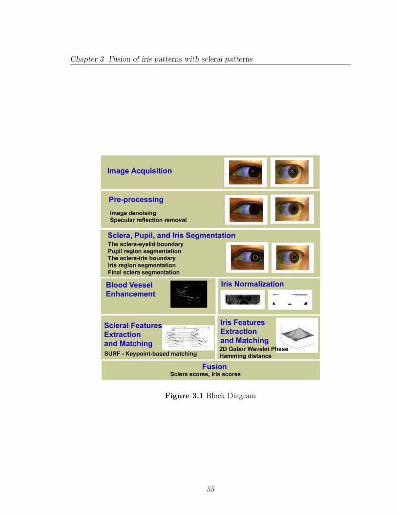
Chapter 3 Fusion of iris patterns with scleral patterns
Figure 3.1 Block Diagram
55
Chapter 3 Fusion of iris patterns with scleral patterns
3.1 Specular reflection detection and removal
The specular reflection (the ring-like shape and the highlights due to the moisture
of the eye) is detected in a two step algorithm and removed by a fast inpainting
procedure. In some images, the ring-like shape may be an incomplete circle, ellipse,
or an arbitrary curved shape with a wide range of intensity values. It may be located
partially in the iris region, its precise detection and removal being more important
especially since the iris texture has to be preserved as much as possible. In the first
step of the algorithm, a good detection of the ring-like shape specular reflection is
accomplished by converting the RGB image into L*a*b color scheme followed by a
range filtering through which every pixel in the image is replaced with the difference
between the maximum and minimum value in a 3− by − 3 neighborhood around the
corresponding pixel. The ring-like shape specular reflection is obtain by applying
a threshold of value th = 30 to the luminance component and it is removed by
morphological dilation and inpainting. The high value of the threshold isolates the
ring-like shape specular reflection from the other highlights. The remaining specular
reflections are detected using different intensity threshold values for each component:
0.8 for NIR, 0.7 for red and 0.8 for green. Only regions with less then 1000 pixels in
size are labeled as specular reflection, are morphologically dilated and inpainted. In
digital inpainting, the information from the boundary of the region to be inpainted
is propagated smoothly inside the region. The value to be inpainted at a pixel is
calculated using a PDE equation 1 in which partial derivatives are replaced by finite
differences between the pixel and its eight neighbors. The final specular reflection
mask consists of the logical OR operation between the masks obtained in two steps.
1http://www.mathworks.com/matlabcentral/fileexchange/4551
56

Chapter 3 Fusion of iris patterns with scleral patterns
3.2 Ocular Region Segmentation
The color image segmentation is a challenging process. It is influenced by illumination,
and the image texture as a result of the saturation, hue and blending of the colors.
Since the scope of the algorithm is to fuse the information provided from the iris and
the sclera, an accurate labeling of pixels pertaining to both regions is very important.
Uneven illumination, the wide variety of intensity values across the eye surface caused
by the curved shape of the eyeball, reflections of the light on the skin surface and
occasionally the presence of plenty of mascara, will make the segmentation of the iris
and the sclera regions a difficult process and even more problematic to achieve in non-
frontal images of the eye. Exposed on the sclera surface, the conjunctival vasculature
appears as dark curved lines, of different thickness that intersect in a random way.
Through the segmentation process they will be distinguished from wrinkles, crows
feet, and eyelashes. It is also important to have an accurate sclera contour along the
eyelids, since the blood vessels may be located on the margins of the sclera. Regardless
of the color of the iris, the algorithm to segment the sclera, the iris and the pupil has
five steps as described below.
1. The sclera-eyelid boundary
2. Pupil region segmentation
3. The sclera-iris boundary
4. Iris region segmentation
5. Final sclera region segmentation
57
Chapter 3 Fusion of iris patterns with scleral patterns
3.2.1 The Sclera-Eyelid Boundary
The algorithm to segment the sclera region presented in Chapter 2 and used in [46]
uses the threshold 0.1 to delineate the pixels pertaining to the sclera region and the
background. The threshold value depends on the illumination of the eye and doesn’t
represent the optimal choice for all the images of the eye. Therefore an improved
automatic segmentation of the sclera region free of thresholds is necessary. The
method employed to segment the sclera region along the eyelid contour is inspired
by the work done in the processing of LandSat imagery (Land + Satellite) [31].
A set of indices, are used to segment the vegetation regions in aerial multispectral
images based on a different absorbtion of the NIR wavelength by regions with different
saturation in water content. Similarly, the index that it’s used for coarse sclera
segmentation is based on the fact that the skin has lesser water content than the
sclera, and hence exhibits a higher reflectance in NIR. Since water absorbs NIR light,
the corresponding regions appear dark in the image and, hence, the sclera appears
darker in the image. The algorithm is as follows:
1. Geometrically resize the near-infrared and green component by a factor of 1/2.
2. Compute an index called the normalized sclera index NSI(x, y) = NIR(x,y)−G(x,y)NIR(x,y)+G(x,y)
,
where NIR(x, y) and G(x, y) are the pixel intensities of the NIR and green
components, respectively, at pixel location (x, y). The difference NIR(x, y) −
G(x, y) is larger for pixels pertaining to the sclera region; it is then normalized
to help compensate for the uneven illumination. Figure 3.2 (b) displays the
normalized sclera index for all three categories as specified by the Martin-Schultz
scale: light colored iris, dark colored iris and mix colored iris.
5. Using the integral image as explained in [36], for each pixel of (x, y) of NSI
compute the mean µ and the standard deviation σ for a neighborhood of radii
58
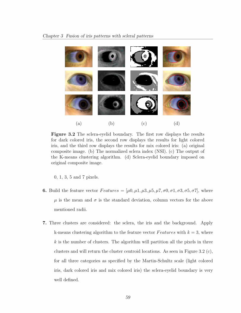
Chapter 3 Fusion of iris patterns with scleral patterns
(a) (b) (c) (d)
Figure 3.2 The sclera-eyelid boundary. The first row displays the resultsfor dark colored iris, the second row displays the results for light colorediris, and the third row displays the results for mix colored iris: (a) originalcomposite image. (b) The normalized sclera index (NSI). (c) The output ofthe K-means clustering algorithm. (d) Sclera-eyelid boundary imposed onoriginal composite image.
0, 1, 3, 5 and 7 pixels.
6. Build the feature vector Features = [µ0, µ1, µ3, µ5, µ7, σ0, σ1, σ3, σ5, σ7], where
µ is the mean and σ is the standard deviation, column vectors for the above
mentioned radii.
7. Three clusters are considered: the sclera, the iris and the background. Apply
k-means clustering algorithm to the feature vector Features with k = 3, where
k is the number of clusters. The algorithm will partition all the pixels in three
clusters and will return the cluster centroid locations. As seen in Figure 3.2 (c),
for all three categories as specified by the Martin-Schultz scale (light colored
iris, dark colored iris and mix colored iris) the sclera-eyelid boundary is very
well defined.
59

Chapter 3 Fusion of iris patterns with scleral patterns
8. For each cluster compute the mean value of all the pixels from NSI image. The
cluster with the lowest mean represents the sclera region. For all three categories
as specified by the Martin-Schultz scale (light colored iris, dark colored iris and
mix colored iris), the sclera cluster exhibits a good segmentation along the
sclera-eyelid boundary, but differs in regard of sclera-iris boundary. For dark
irides (brown and dark brown), the sclera region excluding the iris is localized
(Figure 3.2(d) the first row, referred henceforth as IS). Thus, in this case, the
sclera-iris boundary is detected, and further segmentation of the sclera and iris
is not required. For light irides (blue, green, etc.), regions pertaining to both the
sclera and iris are segmented (Figure 3.2 (d) the second row, referred henceforth
as IS). Here, further separation of the sclera and iris is needed. For mixed irides
(blue or green with brown around pupil), the region of the sclera and the light
colored portion of the iris are segmented as one region (referred henceforth as
IS). The dark portion of the iris (brown) is not included (Figure 3.2(d) the third
row). Here, further separation of the sclera and the portion of the iris is needed.
To find the boundary between the sclera and the iris regardless of the color of
the iris, the pupil is detected. The convex hull of the segmented region IS and
the pupil region will contain the sclera, the pupil, and the iris or the portion of
the iris. This region is referred to as ISIP and is further processed. Since the
proposed algorithm does not deduce the color of the iris, it is applicable to all
images irrespective of the eye color. As seen in Figures 3.2 (c), the location of
the pupil is also visible as part of the sclera cluster in dark and mixed irides, or
as a lighter disk within the sclera region in light irides. This information can be
exploited only if the color of the iris is known in advance. Therefore, in Section
3.2.2 we present an automatic way of finding the pupil location regardless of
the color of the iris.
60
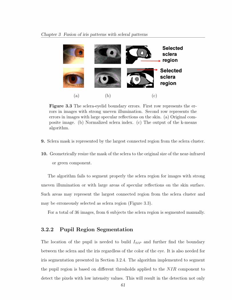
Chapter 3 Fusion of iris patterns with scleral patterns
(a) (b) (c)
Figure 3.3 The sclera-eyelid boundary errors. First row represents the er-rors in images with strong uneven illumination. Second row represents theerrors in images with large specular reflections on the skin. (a) Original com-posite image. (b) Normalized sclera index. (c) The output of the k-meansalgorithm.
9. Sclera mask is represented by the largest connected region from the sclera cluster.
10. Geometrically resize the mask of the sclera to the original size of the near-infrared
or green component.
The algorithm fails to segment properly the sclera region for images with strong
uneven illumination or with large areas of specular reflections on the skin surface.
Such areas may represent the largest connected region from the sclera cluster and
may be erroneously selected as sclera region (Figure 3.3).
For a total of 36 images, from 6 subjects the sclera region is segmented manually.
3.2.2 Pupil Region Segmentation
The location of the pupil is needed to build ISIP and further find the boundary
between the sclera and the iris regardless of the color of the eye. It is also needed for
iris segmentation presented in Section 3.2.4. The algorithm implemented to segment
the pupil region is based on different thresholds applied to the NIR component to
detect the pixels with low intensity values. This will result in the detection not only
61
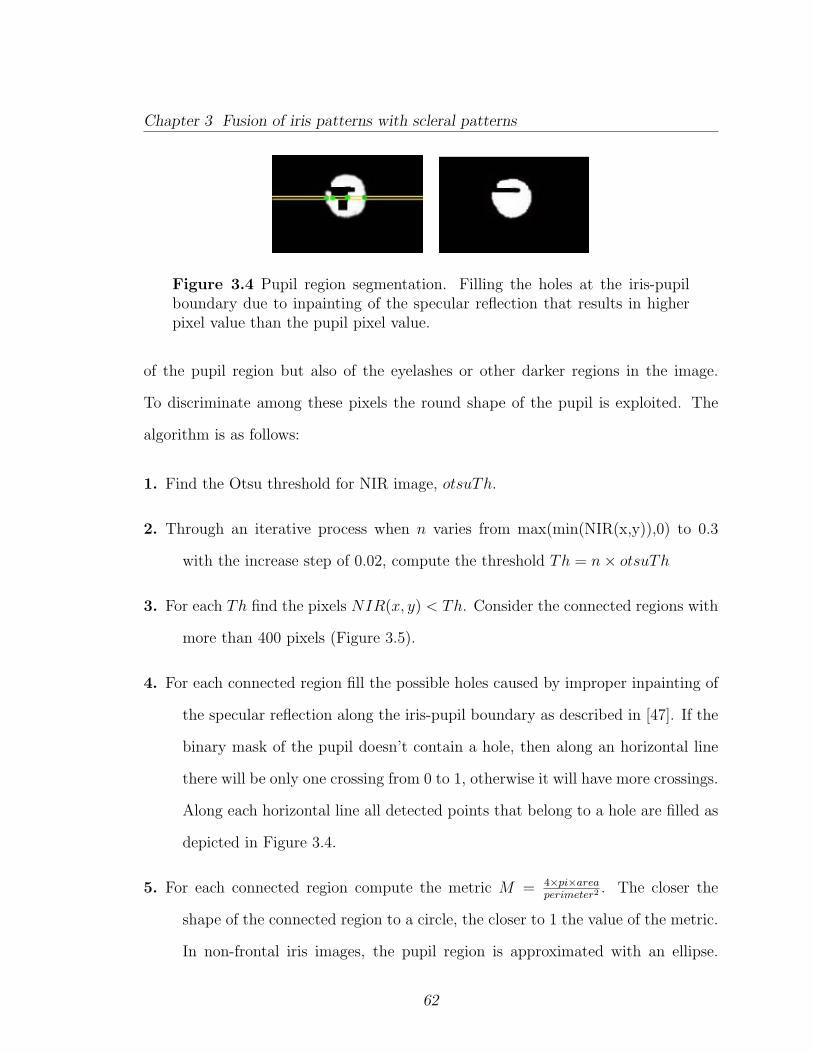
Chapter 3 Fusion of iris patterns with scleral patterns
Figure 3.4 Pupil region segmentation. Filling the holes at the iris-pupilboundary due to inpainting of the specular reflection that results in higherpixel value than the pupil pixel value.
of the pupil region but also of the eyelashes or other darker regions in the image.
To discriminate among these pixels the round shape of the pupil is exploited. The
algorithm is as follows:
1. Find the Otsu threshold for NIR image, otsuTh.
2. Through an iterative process when n varies from max(min(NIR(x,y)),0) to 0.3
with the increase step of 0.02, compute the threshold Th = n× otsuTh
3. For each Th find the pixels NIR(x, y) < Th. Consider the connected regions with
more than 400 pixels (Figure 3.5).
4. For each connected region fill the possible holes caused by improper inpainting of
the specular reflection along the iris-pupil boundary as described in [47]. If the
binary mask of the pupil doesn’t contain a hole, then along an horizontal line
there will be only one crossing from 0 to 1, otherwise it will have more crossings.
Along each horizontal line all detected points that belong to a hole are filled as
depicted in Figure 3.4.
5. For each connected region compute the metric M = 4×pi×areaperimeter2
. The closer the
shape of the connected region to a circle, the closer to 1 the value of the metric.
In non-frontal iris images, the pupil region is approximated with an ellipse.
62

Chapter 3 Fusion of iris patterns with scleral patterns
Since the pupil is not a very elongated ellipse, the metric M will have a value
close to 1.
6. Choose the connected region with the highest value of the metric M . This rep-
resents the contour of the pupil region. Find its contour and fit an ellipse
Epupil(xp, yp,Mp,mp, θp) where (xp, yp) represents the center coordinates of the
ellipse, Mp,mp represents the major and minor axes and θp represents the tilt
of the ellipse.
Since the value of the metric M is based on the area and perimeter values, the
algorithm fails to properly segment the pupil region if by inpainting a large specu-
lar reflection area located at the boundary between the pupil and the iris, changes
drastically the elliptical contour of the pupil. In such cases the failure to segment
properly the pupil region is accentuated by heavy mascara on the eyelashes. To solve
this problem, constraints on pupil location may be added to the algorithm to improve
the segmentation performance such as considering only half the image, according to
the gaze direction or locate the pupil region in the ellipse mask fitted to the sclera
region as described in Chapter 2 and used in [48] (The contour of the convex hull of
the sclera region is detected. Using Hough transform for line detection, the highest
peak corresponding to the longest line is selected and removed. An ellipse is fitted
to the remaining contour pixels. The search for the pupil region is constraint among
the pixels located within the fitted ellipse).
Example of images with segmented pupil region are displayed in Figure 3.6
For a total of 19 images pertaining to 6 subjects, the pupil is segmented automat-
ically.
63
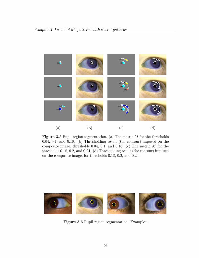
Chapter 3 Fusion of iris patterns with scleral patterns
0.44
0.18
0.84
0.55
0.83
0.22
0.84
0.49
0.23
0.78
0.55 0.14
0.88
(a) (b) (c) (d)
Figure 3.5 Pupil region segmentation. (a) The metric M for the thresholds0.04, 0.1, and 0.16. (b) Thresholding result (the contour) imposed on thecomposite image, thresholds 0.04, 0.1, and 0.16. (c) The metric M for thethresholds 0.18, 0.2, and 0.24. (d) Thresholding result (the contour) imposedon the composite image, for thresholds 0.18, 0.2, and 0.24.
Figure 3.6 Pupil region segmentation. Examples.
64
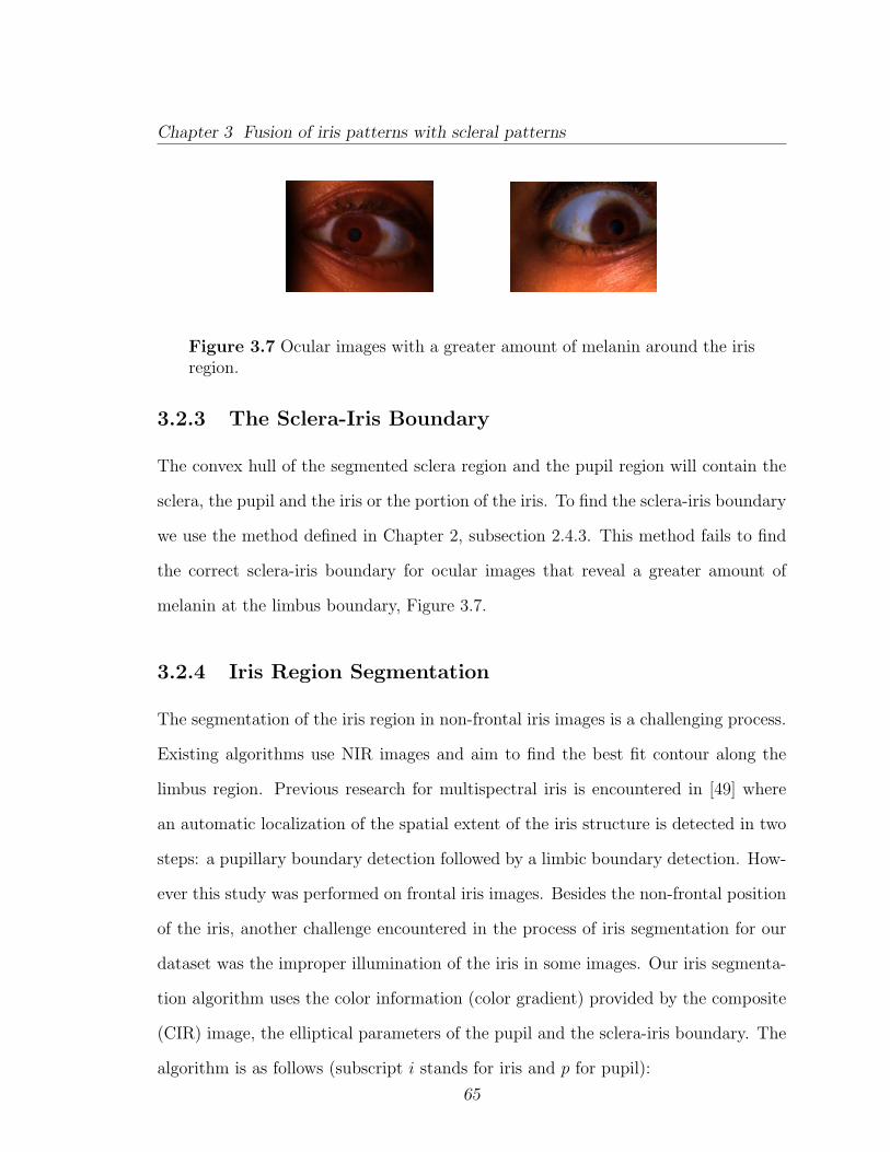
Chapter 3 Fusion of iris patterns with scleral patterns
Figure 3.7 Ocular images with a greater amount of melanin around the irisregion.
3.2.3 The Sclera-Iris Boundary
The convex hull of the segmented sclera region and the pupil region will contain the
sclera, the pupil and the iris or the portion of the iris. To find the sclera-iris boundary
we use the method defined in Chapter 2, subsection 2.4.3. This method fails to find
the correct sclera-iris boundary for ocular images that reveal a greater amount of
melanin at the limbus boundary, Figure 3.7.
3.2.4 Iris Region Segmentation
The segmentation of the iris region in non-frontal iris images is a challenging process.
Existing algorithms use NIR images and aim to find the best fit contour along the
limbus region. Previous research for multispectral iris is encountered in [49] where
an automatic localization of the spatial extent of the iris structure is detected in two
steps: a pupillary boundary detection followed by a limbic boundary detection. How-
ever this study was performed on frontal iris images. Besides the non-frontal position
of the iris, another challenge encountered in the process of iris segmentation for our
dataset was the improper illumination of the iris in some images. Our iris segmenta-
tion algorithm uses the color information (color gradient) provided by the composite
(CIR) image, the elliptical parameters of the pupil and the sclera-iris boundary. The
algorithm is as follows (subscript i stands for iris and p for pupil):
65

Chapter 3 Fusion of iris patterns with scleral patterns
1. Using the parameters of the ellipse that fit the contour of the pupil, unwrap the
sclera mask. The angular resolution is ang res = 360 and the radial resolution is
rad res = radius/res where res = 120 and radius is of variable size according
to the dilation of the pupil. To detect the best radial resolution, through an
iterative process and starting with the value radius = 3, the radius is increased
by 1 and sclera mask unwrapped for each iteration. The number of pixels
pertaining to the unwrapped sclera mask along the lines is computed and the
maximum value is detected. The iterative process stops when the location of
the maximum value is greater then res − 10. This is based on the fact that
as the sclera mask is unwrapped, the shape of the unwrapped sclera can be
approximated with that of a trapezoid with the larger base up. The value of
the resolution rad res is very important for the ratios calculated in the next
steps. The results are depicted in Figure 3.9 (b). The sclera region is represented
by the white region. To better visualize the location of the iris, pupil, and sclera
region in the unwrapped sclera mask and pupil mask, the composite images from
Figure 3.2 (a), representing the three categories in the Martin-Schultz scale, are
unwrapped and displayed in Figure 3.8.
2. Using the parameters of the ellipse that fit the contour of the pupil, elliptical
unwrap the pupil mask with the determined angular and the radial resolutions.
The results are depicted in Figure 3.9 (a). The pupil region is represented by
the gray region. Since the pupil parameters are used to unwrap the pupil mask,
the iris-pupil boundary is represented by a straight line. Find the pupil-iris
boundary Bpi.
3. Since the pupil parameters are used to unwrap the sclera mask, the sclera-iris
boundary is represented by a a curved line as displayed with yellow color in
66

Chapter 3 Fusion of iris patterns with scleral patterns
Figure 3.9 (b). Find two lines Bsimin (red color) and Bsimax (blue color) corre-
sponding to the minimum and the maximum position of the sclera-iris boundary
(the yellow line). Two ratios are calculated Rmin and Rmax, in order to find the
parameters of two ellipses, Emin and Emax, used to approximate the contour of
the iris region.
Rmin = Bsimin
Bpi,
Rmax = Bsimax
Bpi
(3.1)
4. Keeping the tilt angle and the center coordinates of the pupil, based on the two
ratios and the pupil’s major and minor axis values, calculate the major and
minor axis of two ellipses Ellipsemin and Ellipsemax, as follows:
Rp = Mp/mp,
mi max = Rmax ×mp,
mi min = Rmin ×mp,
Mi min = Rp ×mi min,
Mi max = Rp ×mi max
(3.2)
The resulting ellipses Emin(xi, yi,Mi min,mi min, θi) and Emax(xi, yi,Mi max,mi max, θi)
, where (xi, yi) = (xp, yp) , and θi = θp, are depicted in Figure 3.10. As it can be
observed, the sclera-iris boundary is in between the two ellipses. The remaining
steps are considered for a more accurate ellipse fitting to the contour of the iris.
5. Build an elliptical mask comprised of all the pixels inside the Emax.
6. Apply the color gradient algorithm to the composite image, Figure 3.11 (a) and
threshold it with Th = 0.1. Impose the elliptical mask on the resulting image.
Results, ImCG, are displayed in Figure 3.11 (b).
67

Chapter 3 Fusion of iris patterns with scleral patterns
7. Using the parameters that fit the contour of the pupil, unwrap the image ImCG
obtained in the previous step.
8. Calculate the sum of all the pixels along the rows and find the maximum value in
between the two lines Bsimin (red color) and Bsimax (blue color).
9. Recalculate the ratios from step 4 and find the major and minor axis for an ellipse
that will best fit the contour of the iris. Build an elliptical mask comprised of
all the pixels inside the ellipse.
10. Find the convex hull of the sclera cluster and the elliptical mask and apply the
hole filling algorithm as used in Section 3.2.2.
11. Similar to the algorithm presented in Chapter 2, Section 2.4.3, apply K-means
algorithm with k = 2 (the sclera and iris clusters) to the pixels inside the convex
hull. Two binary images, a mask for the sclera region and a mask for the iris
region represent the output.
12. Pixels pertaining to the sclera region, mostly those along the upper eyelid con-
tour, may be labeled as iris pixels. Therefore, from the center of the pupil,
build a set of rays to the contour of the iris mask and consider always the first
intersection of the ray with the iris contour. This will provide the final iris
contour. Fit an ellipse to this contour.
13. Find the maximum and minimum values along the x coordinate of the sclera
mask and limit the iris mask in between these to values.
Examples of images with segmented iris are displayed in Figure 3.13.
The algorithm returns error to segment the iris in 12 images. For these images,
the iris is segmented manually. Approximately 85% of the times the generated ellipse
will fit the boundary region of the iris for both eyes both gaze directions.
68
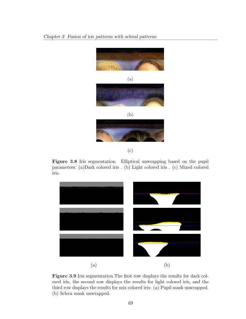
Chapter 3 Fusion of iris patterns with scleral patterns
(a)
(b)
(c)
Figure 3.8 Iris segmentation. Elliptical unwrapping based on the pupilparameters: (a)Dark colored iris . (b) Light colored iris . (c) Mixed colorediris.
(a) (b)
Figure 3.9 Iris segmentation.The first row displays the results for dark col-ored iris, the second row displays the results for light colored iris, and thethird row displays the results for mix colored iris: (a) Pupil mask unwrapped.(b) Sclera mask unwrapped.
69
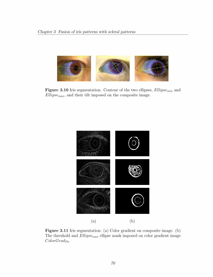
Chapter 3 Fusion of iris patterns with scleral patterns
Figure 3.10 Iris segmentation. Contour of the two ellipses, Ellipsemin andEllipsemax, and their tilt imposed on the composite image.
(a) (b)
Figure 3.11 Iris segmentation: (a) Color gradient on composite image. (b)The threshold and Ellipsemax ellipse mask imposed on color gradient imageColorGradTh.
70
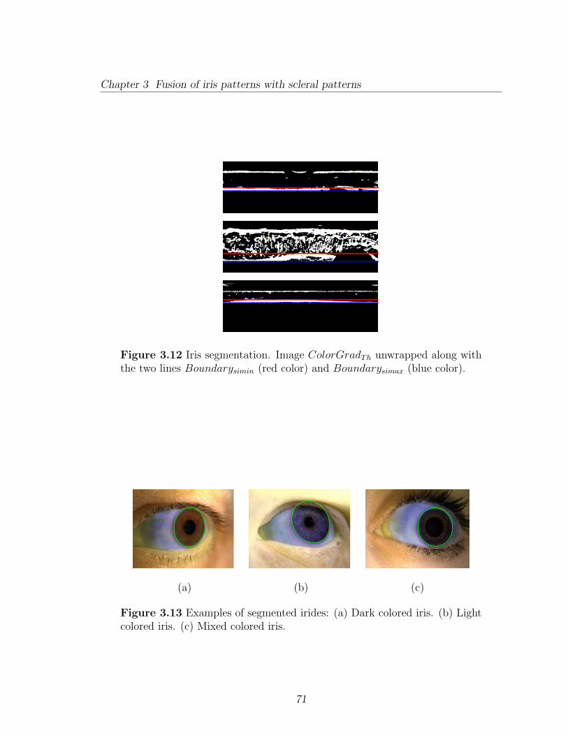
Chapter 3 Fusion of iris patterns with scleral patterns
Figure 3.12 Iris segmentation. Image ColorGradTh unwrapped along withthe two lines Boundarysimin (red color) and Boundarysimax (blue color).
(a) (b) (c)
Figure 3.13 Examples of segmented irides: (a) Dark colored iris. (b) Lightcolored iris. (c) Mixed colored iris.
71
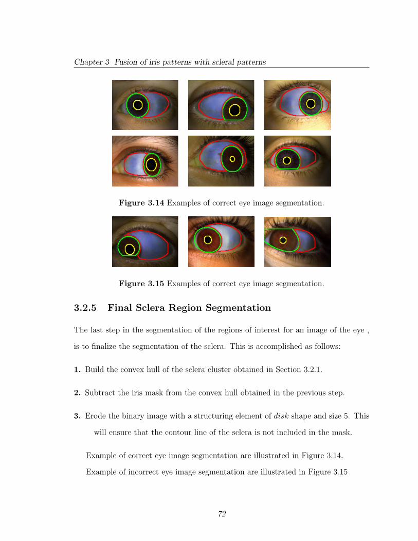
Chapter 3 Fusion of iris patterns with scleral patterns
Figure 3.14 Examples of correct eye image segmentation.
Figure 3.15 Examples of correct eye image segmentation.
3.2.5 Final Sclera Region Segmentation
The last step in the segmentation of the regions of interest for an image of the eye ,
is to finalize the segmentation of the sclera. This is accomplished as follows:
1. Build the convex hull of the sclera cluster obtained in Section 3.2.1.
2. Subtract the iris mask from the convex hull obtained in the previous step.
3. Erode the binary image with a structuring element of disk shape and size 5. This
will ensure that the contour line of the sclera is not included in the mask.
Example of correct eye image segmentation are illustrated in Figure 3.14.
Example of incorrect eye image segmentation are illustrated in Figure 3.15
72
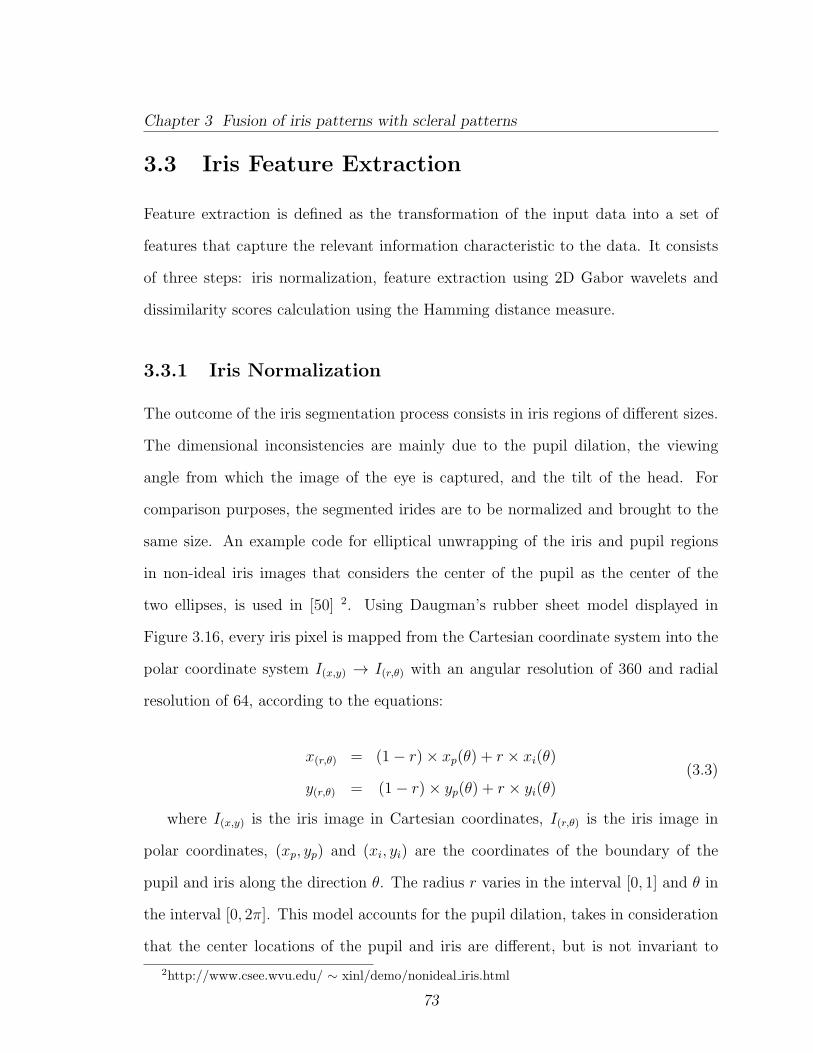
Chapter 3 Fusion of iris patterns with scleral patterns
3.3 Iris Feature Extraction
Feature extraction is defined as the transformation of the input data into a set of
features that capture the relevant information characteristic to the data. It consists
of three steps: iris normalization, feature extraction using 2D Gabor wavelets and
dissimilarity scores calculation using the Hamming distance measure.
3.3.1 Iris Normalization
The outcome of the iris segmentation process consists in iris regions of different sizes.
The dimensional inconsistencies are mainly due to the pupil dilation, the viewing
angle from which the image of the eye is captured, and the tilt of the head. For
comparison purposes, the segmented irides are to be normalized and brought to the
same size. An example code for elliptical unwrapping of the iris and pupil regions
in non-ideal iris images that considers the center of the pupil as the center of the
two ellipses, is used in [50] 2. Using Daugman’s rubber sheet model displayed in
Figure 3.16, every iris pixel is mapped from the Cartesian coordinate system into the
polar coordinate system I(x,y) → I(r,θ) with an angular resolution of 360 and radial
resolution of 64, according to the equations:
x(r,θ) = (1− r)× xp(θ) + r × xi(θ)
y(r,θ) = (1− r)× yp(θ) + r × yi(θ)(3.3)
where I(x,y) is the iris image in Cartesian coordinates, I(r,θ) is the iris image in
polar coordinates, (xp, yp) and (xi, yi) are the coordinates of the boundary of the
pupil and iris along the direction θ. The radius r varies in the interval [0, 1] and θ in
the interval [0, 2π]. This model accounts for the pupil dilation, takes in consideration
that the center locations of the pupil and iris are different, but is not invariant to
2http://www.csee.wvu.edu/ ∼ xinl/demo/nonideal iris.html
73
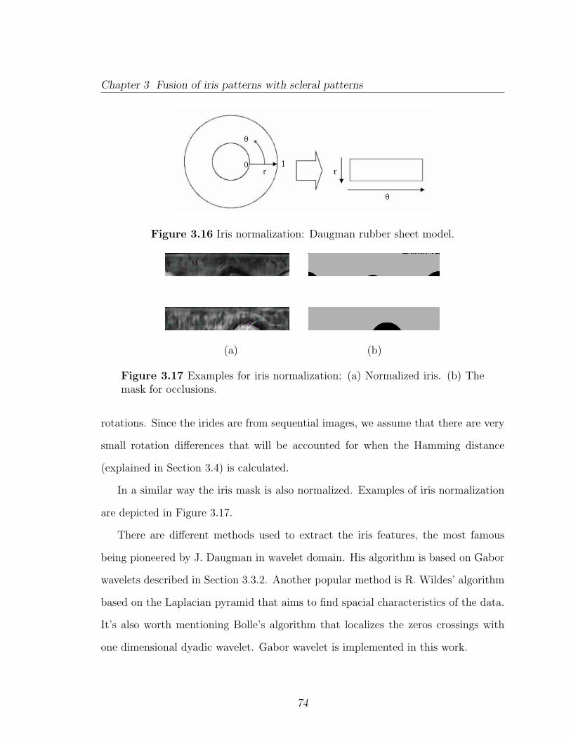
Chapter 3 Fusion of iris patterns with scleral patterns
Figure 3.16 Iris normalization: Daugman rubber sheet model.
(a) (b)
Figure 3.17 Examples for iris normalization: (a) Normalized iris. (b) Themask for occlusions.
rotations. Since the irides are from sequential images, we assume that there are very
small rotation differences that will be accounted for when the Hamming distance
(explained in Section 3.4) is calculated.
In a similar way the iris mask is also normalized. Examples of iris normalization
are depicted in Figure 3.17.
There are different methods used to extract the iris features, the most famous
being pioneered by J. Daugman in wavelet domain. His algorithm is based on Gabor
wavelets described in Section 3.3.2. Another popular method is R. Wildes’ algorithm
based on the Laplacian pyramid that aims to find spacial characteristics of the data.
It’s also worth mentioning Bolle’s algorithm that localizes the zeros crossings with
one dimensional dyadic wavelet. Gabor wavelet is implemented in this work.
74
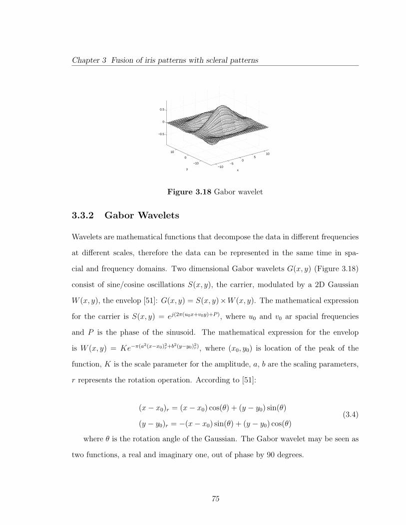
Chapter 3 Fusion of iris patterns with scleral patterns
−10−5
05
10
−10
0
10
−0.5
0
0.5
xy
Figure 3.18 Gabor wavelet
3.3.2 Gabor Wavelets
Wavelets are mathematical functions that decompose the data in different frequencies
at different scales, therefore the data can be represented in the same time in spa-
cial and frequency domains. Two dimensional Gabor wavelets G(x, y) (Figure 3.18)
consist of sine/cosine oscillations S(x, y), the carrier, modulated by a 2D Gaussian
W (x, y), the envelop [51]: G(x, y) = S(x, y)×W (x, y). The mathematical expression
for the carrier is S(x, y) = ej(2π(u0x+v0y)+P ), where u0 and v0 ar spacial frequencies
and P is the phase of the sinusoid. The mathematical expression for the envelop
is W (x, y) = Ke−π(a2(x−x0)2r+b2(y−y0)2r), where (x0, y0) is location of the peak of the
function, K is the scale parameter for the amplitude, a, b are the scaling parameters,
r represents the rotation operation. According to [51]:
(x− x0)r = (x− x0) cos(θ) + (y − y0) sin(θ)
(y − y0)r = −(x− x0) sin(θ) + (y − y0) cos(θ)(3.4)
where θ is the rotation angle of the Gaussian. The Gabor wavelet may be seen as
two functions, a real and imaginary one, out of phase by 90 degrees.
75
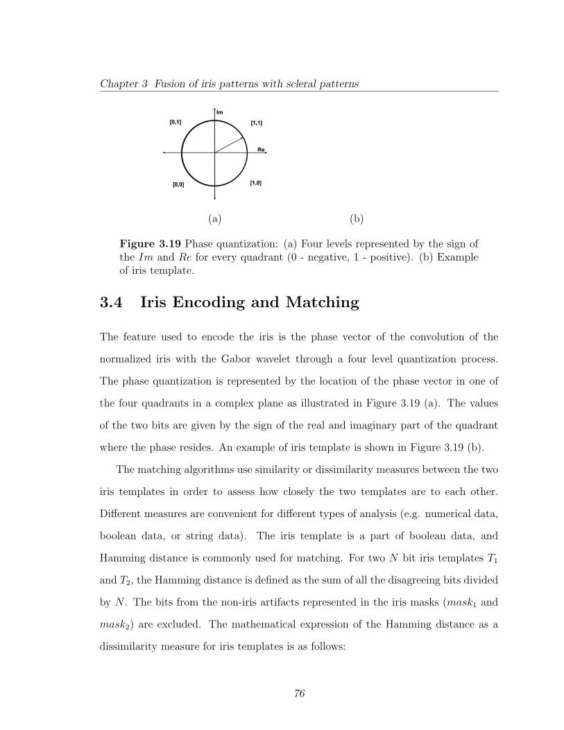
Chapter 3 Fusion of iris patterns with scleral patterns
(a) (b)
Figure 3.19 Phase quantization: (a) Four levels represented by the sign ofthe Im and Re for every quadrant (0 - negative, 1 - positive). (b) Exampleof iris template.
3.4 Iris Encoding and Matching
The feature used to encode the iris is the phase vector of the convolution of the
normalized iris with the Gabor wavelet through a four level quantization process.
The phase quantization is represented by the location of the phase vector in one of
the four quadrants in a complex plane as illustrated in Figure 3.19 (a). The values
of the two bits are given by the sign of the real and imaginary part of the quadrant
where the phase resides. An example of iris template is shown in Figure 3.19 (b).
The matching algorithms use similarity or dissimilarity measures between the two
iris templates in order to assess how closely the two templates are to each other.
Different measures are convenient for different types of analysis (e.g. numerical data,
boolean data, or string data). The iris template is a part of boolean data, and
Hamming distance is commonly used for matching. For two N bit iris templates T1
and T2, the Hamming distance is defined as the sum of all the disagreeing bits divided
by N . The bits from the non-iris artifacts represented in the iris masks (mask1 and
mask2) are excluded. The mathematical expression of the Hamming distance as a
dissimilarity measure for iris templates is as follows:
76

Chapter 3 Fusion of iris patterns with scleral patterns
HD =
∑Ni=1(T1i ⊕ T2i ∩mask1i ∩mask2i)
N(3.5)
3.5 Sclera Feature Extraction and Matching
The conjunctival vasculature displayed on the sclera surface is enhanced using selec-
tive enhancement filter for lines. The algorithm is described in Chapter 2, Section
2.5. The use of keypoint-based matching method (SURF) described in Chapter 2,
Section 2.7.1 was observed to result in the best recognition performance for the scleral
patterns. Therefore this method is further used to combine the iris patterns with the
sclera patterns.
3.6 Results
The ROC and the distribution of scores for all methods employed in this chapter
such as SURF, Hamming distance and the score level fusion of iris patterns and
scleral patterns, for left and right eye, both gaze directions are depicted in Appendix
B. Table 3.1 shows the results of the Hamming distance dissimilarity measure. The
best performance of iris recognition is obtained for left-eye-looking-left (L L) and
right-eye-looking-right (R R) with EER values of less then 1%. In the case of left-eye-
looking right (L R) and right-eye-looking-left (R L) where the light that reaches the
eye is obstructed by the facial structure (the nose) and is directed as much as possible
towards the sclera region, the EER values of 3.5% show a decrease is performance for
iris recognition.
Table 3.2 displays the results for interest point matching SURF applied to the
pre-processed images of the sclera. The results are promising; the EER values are in
77
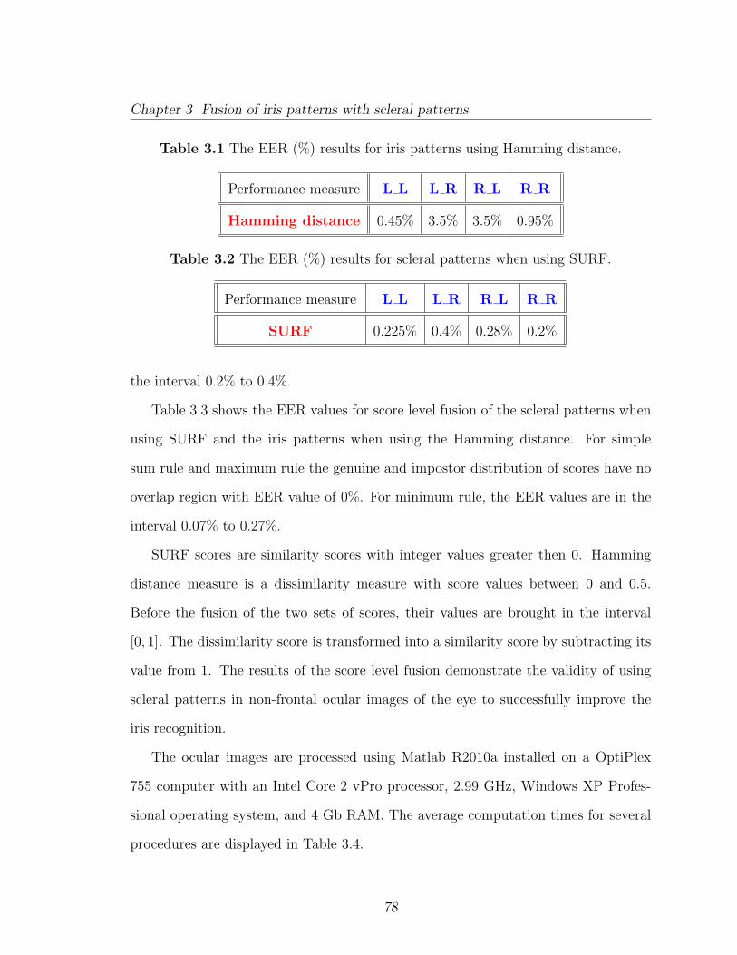
Chapter 3 Fusion of iris patterns with scleral patterns
Table 3.1 The EER (%) results for iris patterns using Hamming distance.
Performance measure L L L R R L R R
Hamming distance 0.45% 3.5% 3.5% 0.95%
Table 3.2 The EER (%) results for scleral patterns when using SURF.
Performance measure L L L R R L R R
SURF 0.225% 0.4% 0.28% 0.2%
the interval 0.2% to 0.4%.
Table 3.3 shows the EER values for score level fusion of the scleral patterns when
using SURF and the iris patterns when using the Hamming distance. For simple
sum rule and maximum rule the genuine and impostor distribution of scores have no
overlap region with EER value of 0%. For minimum rule, the EER values are in the
interval 0.07% to 0.27%.
SURF scores are similarity scores with integer values greater then 0. Hamming
distance measure is a dissimilarity measure with score values between 0 and 0.5.
Before the fusion of the two sets of scores, their values are brought in the interval
[0, 1]. The dissimilarity score is transformed into a similarity score by subtracting its
value from 1. The results of the score level fusion demonstrate the validity of using
scleral patterns in non-frontal ocular images of the eye to successfully improve the
iris recognition.
The ocular images are processed using Matlab R2010a installed on a OptiPlex
755 computer with an Intel Core 2 vPro processor, 2.99 GHz, Windows XP Profes-
sional operating system, and 4 Gb RAM. The average computation times for several
procedures are displayed in Table 3.4.
78
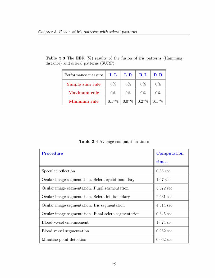
Chapter 3 Fusion of iris patterns with scleral patterns
Table 3.3 The EER (%) results of the fusion of iris patterns (Hammingdistance) and scleral patterns (SURF).
Performance measure L L L R R L R R
Simple sum rule 0% 0% 0% 0%
Maximum rule 0% 0% 0% 0%
Minimum rule 0.17% 0.07% 0.27% 0.17%
Table 3.4 Average computation times
Procedure Computation
times
Specular reflection 0.65 sec
Ocular image segmentation. Sclera-eyelid boundary 1.67 sec
Ocular image segmentation. Pupil segmentation 3.672 sec
Ocular image segmentation. Sclera-iris boundary 2.631 sec
Ocular image segmentation. Iris segmentation 4.314 sec
Ocular image segmentation. Final sclera segmentation 0.645 sec
Blood vessel enhancement 1.674 sec
Blood vessel segmentation 0.952 sec
Minutiae point detection 0.062 sec
79
Chapter 3 Fusion of iris patterns with scleral patterns
3.7 Summary
The work presented in this chapter aims to demonstrate the potential of designing a
bimodal ocular system that combines sclera biometric with the iris biometric. The
ocular images of the first collection of the multispectral database are denoised and
further pre-processed to detect and remove the specular reflections. An automatic
sclera region segmentation was designed to localize the spatial extent of the iris, sclera
and pupil regions in the ocular images. The proposed segmentation algorithm is a
combination of region-based and edge-based schemes that exploits the multispectral
information. The use of keypoint-based matching was observed to result in the best
recognition performance for the scleral patterns. Therefore, Speeded Up Robust
Features is used to asses the performance of scleral patterns as biometric cue. Using
elliptical unwrapping, the segmented iris is normalized and encoded using 2D Gabor
filters. Hamming distance is used as a dissimilarity measure to asses the performance
of iris recognition. The sclera scores and the iris scores are combined at a score
level using three fusion rules: simple sum rule, maximum rule and minimum rule.
The results show an improvement of the EER mainly for the simple sum rule and
maximum rule when the genuine and impostor distribution scores are totaly non-
overlapping. This suggests that when looking to the left or looking to the right,
the information gained from the exposed sclera texture may be used to improve the
performance of non-frontal iris recognition.
80
Chapter 4
Impact of intra-class variation
The previous approaches demonstrate the validity of using the sclera texture and the
conjunctival vasculature exhibited on its surface as a biometric cue and the benefit
gained from the fusion of iris patterns with sclera patterns in non-ideal images of the
eye. The ocular images were obtained in a constraint environment, with controlled
lighting conditions and distance to the camera. The selection of eight consecutive
frames ensured that the viewing angle is approximately the same for all eight images.
The results are promising and suggest further insight into addressing the remaining
challenges. However, the selection of the consecutive frames resulted in less intra-
class variation. The work in this chapter investigates the potential of using the sclera
texture and the blood vessels as a biometric cue for ocular images with increased
intra-class variation. This is accomplished by using the ocular images of the second
collection from the multispectral database presented in Chapter 2, Section 2.1.
The block diagram of the proposed system is shown in Figure 4.1.
After acquisition presented in Chapter 2, Section 2.1, the ocular images are de-
noised using wavelet transform as presented in Chapter 2, Section 2.2. The specular
reflection is detected and removed with the two step algorithm presented in Chapter 3,
81
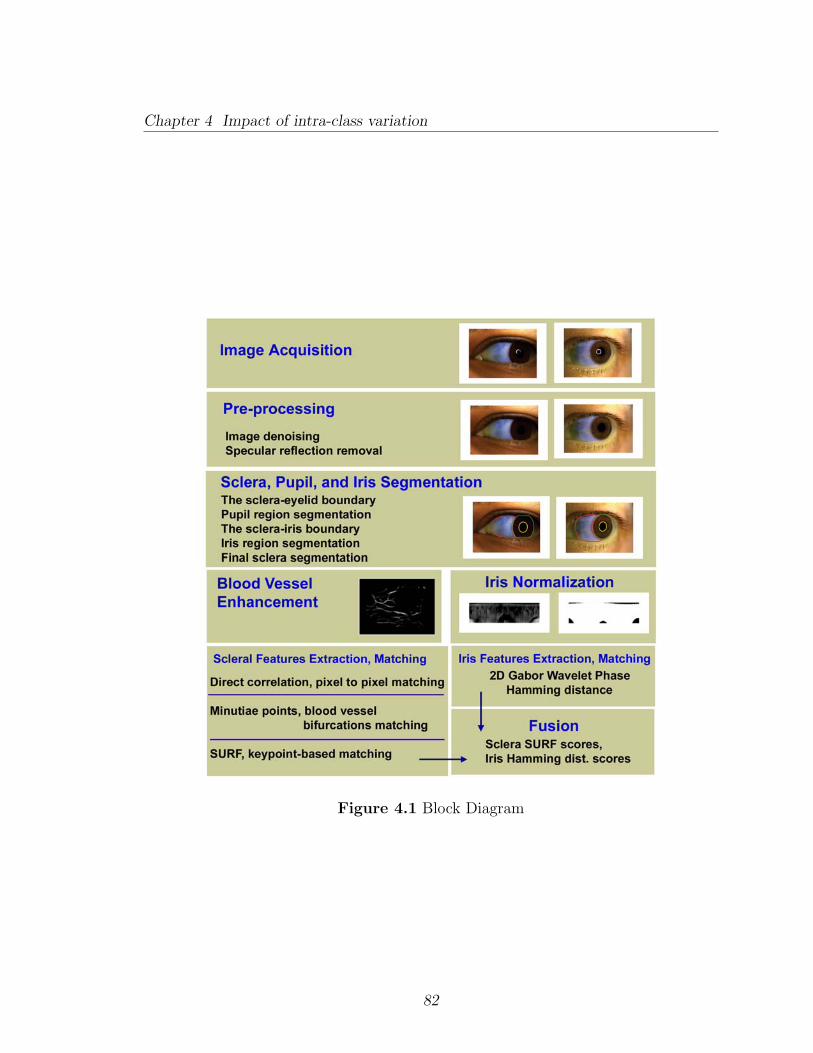
Chapter 4 Impact of intra-class variation
Figure 4.1 Block Diagram
82

Chapter 4 Impact of intra-class variation
Section 3.1. The sclera, the pupil and the iris are segmented using the automatic
segmentation algorithm, a combination of region-based and edge-based schemes as
described in Chapter 3, Section 3.2. The conjunctival vasculature seen on the seg-
mented sclera region is enhanced using the selective enhancement filter for lines as
in Chapter 2, Section 2.5 and the pre-processed images are registered as described in
Chapter 2, Section 2.6. The three feature extraction and matching techniques men-
tioned in Chapter 2, Section 2.7, the keypoint-based matching (SURF), pixel to pixel
matching (direct correlation matching - CORR, MI, NMI, RMSE, RIU, SSIM) and
the bifurcations of the blood vessels matching (minutiae points) are applied to the
pre-processed or registered images of the sclera region. Based on elliptical unwrapping
algorithm mentioned in Chapter 3, Section 3.3.1, the iris is normalized, and then en-
coded using 2D Gabor wavelet as in Section 3.3.2 and 3.4. Hamming distance is used
to assess the performance of iris recognition. As observed in the previous chapters the
keypoint-based matching was observed to result in the best recognition performance
for scleral patterns. Therefore the fusion of the iris patterns with the sclera patterns
is realized by combining the sclera scores obtained with Speeded Up Robust Features
(SURF) and the iris scores obtained with Hamming distance dissimilarity measure.
4.1 Results
The ROC and the distribution of scores for all the methods used in this chapter are
depicted in Appendix C. As observed from the Table 4.1, for ocular images of the
eye with increased intra-class variation there is little change in performance when
using keypoint-based matching (SURF) technique. The values of EER are slightly
increased from 0.2% to 0.8% for right-eye-looking-right (R R), but slightly decreased
from around 0.2% to 0.1% for left-eye-looking-left (L L) and right-eye-looking-left
83
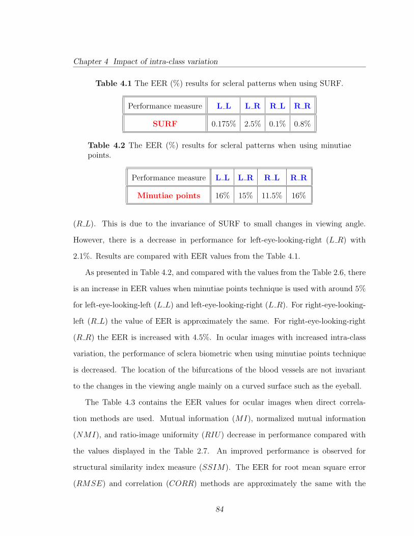
Chapter 4 Impact of intra-class variation
Table 4.1 The EER (%) results for scleral patterns when using SURF.
Performance measure L L L R R L R R
SURF 0.175% 2.5% 0.1% 0.8%
Table 4.2 The EER (%) results for scleral patterns when using minutiaepoints.
Performance measure L L L R R L R R
Minutiae points 16% 15% 11.5% 16%
(R L). This is due to the invariance of SURF to small changes in viewing angle.
However, there is a decrease in performance for left-eye-looking-right (L R) with
2.1%. Results are compared with EER values from the Table 4.1.
As presented in Table 4.2, and compared with the values from the Table 2.6, there
is an increase in EER values when minutiae points technique is used with around 5%
for left-eye-looking-left (L L) and left-eye-looking-right (L R). For right-eye-looking-
left (R L) the value of EER is approximately the same. For right-eye-looking-right
(R R) the EER is increased with 4.5%. In ocular images with increased intra-class
variation, the performance of sclera biometric when using minutiae points technique
is decreased. The location of the bifurcations of the blood vessels are not invariant
to the changes in the viewing angle mainly on a curved surface such as the eyeball.
The Table 4.3 contains the EER values for ocular images when direct correla-
tion methods are used. Mutual information (MI), normalized mutual information
(NMI), and ratio-image uniformity (RIU) decrease in performance compared with
the values displayed in the Table 2.7. An improved performance is observed for
structural similarity index measure (SSIM). The EER for root mean square error
(RMSE) and correlation (CORR) methods are approximately the same with the
84
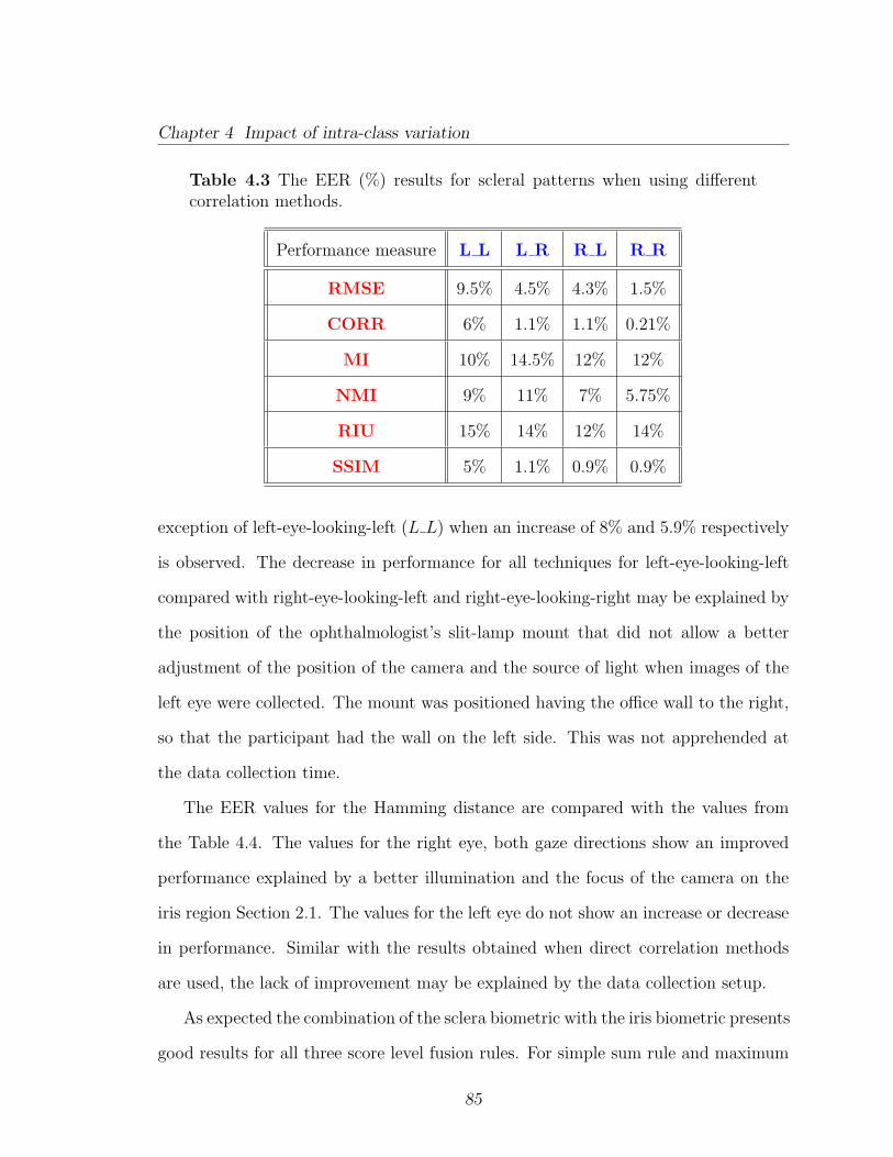
Chapter 4 Impact of intra-class variation
Table 4.3 The EER (%) results for scleral patterns when using differentcorrelation methods.
Performance measure L L L R R L R R
RMSE 9.5% 4.5% 4.3% 1.5%
CORR 6% 1.1% 1.1% 0.21%
MI 10% 14.5% 12% 12%
NMI 9% 11% 7% 5.75%
RIU 15% 14% 12% 14%
SSIM 5% 1.1% 0.9% 0.9%
exception of left-eye-looking-left (L L) when an increase of 8% and 5.9% respectively
is observed. The decrease in performance for all techniques for left-eye-looking-left
compared with right-eye-looking-left and right-eye-looking-right may be explained by
the position of the ophthalmologist’s slit-lamp mount that did not allow a better
adjustment of the position of the camera and the source of light when images of the
left eye were collected. The mount was positioned having the office wall to the right,
so that the participant had the wall on the left side. This was not apprehended at
the data collection time.
The EER values for the Hamming distance are compared with the values from
the Table 4.4. The values for the right eye, both gaze directions show an improved
performance explained by a better illumination and the focus of the camera on the
iris region Section 2.1. The values for the left eye do not show an increase or decrease
in performance. Similar with the results obtained when direct correlation methods
are used, the lack of improvement may be explained by the data collection setup.
As expected the combination of the sclera biometric with the iris biometric presents
good results for all three score level fusion rules. For simple sum rule and maximum
85
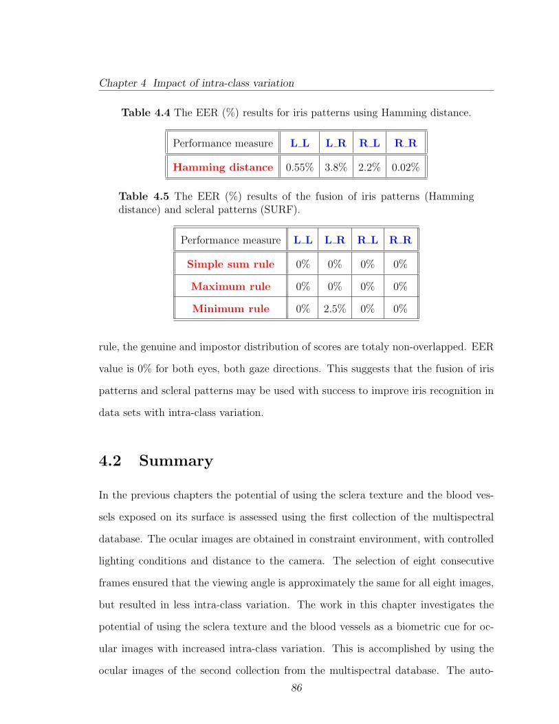
Chapter 4 Impact of intra-class variation
Table 4.4 The EER (%) results for iris patterns using Hamming distance.
Performance measure L L L R R L R R
Hamming distance 0.55% 3.8% 2.2% 0.02%
Table 4.5 The EER (%) results of the fusion of iris patterns (Hammingdistance) and scleral patterns (SURF).
Performance measure L L L R R L R R
Simple sum rule 0% 0% 0% 0%
Maximum rule 0% 0% 0% 0%
Minimum rule 0% 2.5% 0% 0%
rule, the genuine and impostor distribution of scores are totaly non-overlapped. EER
value is 0% for both eyes, both gaze directions. This suggests that the fusion of iris
patterns and scleral patterns may be used with success to improve iris recognition in
data sets with intra-class variation.
4.2 Summary
In the previous chapters the potential of using the sclera texture and the blood ves-
sels exposed on its surface is assessed using the first collection of the multispectral
database. The ocular images are obtained in constraint environment, with controlled
lighting conditions and distance to the camera. The selection of eight consecutive
frames ensured that the viewing angle is approximately the same for all eight images,
but resulted in less intra-class variation. The work in this chapter investigates the
potential of using the sclera texture and the blood vessels as a biometric cue for oc-
ular images with increased intra-class variation. This is accomplished by using the
ocular images of the second collection from the multispectral database. The auto-
86
Chapter 4 Impact of intra-class variation
matic segmentation algorithm is used to localize the iris, sclera and pupil regions.
Conjunctival vasculature is enhanced using the selective line enhancement filters for
lines and pre-processed images of the sclera are registered as described in previous
chapters. The three feature extraction methods, keypoint-based matching, direct cor-
relation methods and minutiae points are applied to the pre-processed images of the
sclera. The results demonstrate an increase of EER for direct correlation methods
and minutiae points method. This is explained by the variance of these methods
to changes in the viewing angle. On the other hand, keypoint-based method SURF
exhibits the same good results. This is explained by the fact that SURF is invariant
to small changes in the viewing angle. Further the score level fusion of scleral pat-
terns and iris patterns when using SURF and Hamming distance, presents the same
good results, proving that the use of scleral patterns combined with iris patterns may
improve the iris recognition in non-frontal images of the eye.
87
Chapter 5
Sclera recognition using low
resolution visible spectrum images
5.1 Visible spectrum data set
The SONY CyberShot DSC F717 (5 megapixels) was used to capture color images of
the eye 1. Each subject was asked to move their eyes in the following manner with
respect to the optical axis of the camera: frontal, upward, to the left and to the right.
Thus different regions of the sclera where represented in the ensuing pictures. These
color images (RGB) were collected in two sessions. The first session had 2400 images
from 50 subjects, and the second session had 816 images from 17 of the original 50
subjects. Images were captured from both eyes at three different distances: 1 foot
considered as near distance images, 9 feet as medium distance images, and 12 feet as
far distance images. For each eye, 2 images were collected per gaze at each distance.
Figure 5.1 displays the four gaze directions for near distance.
1Collected at University of Missouri, Kansas City
88
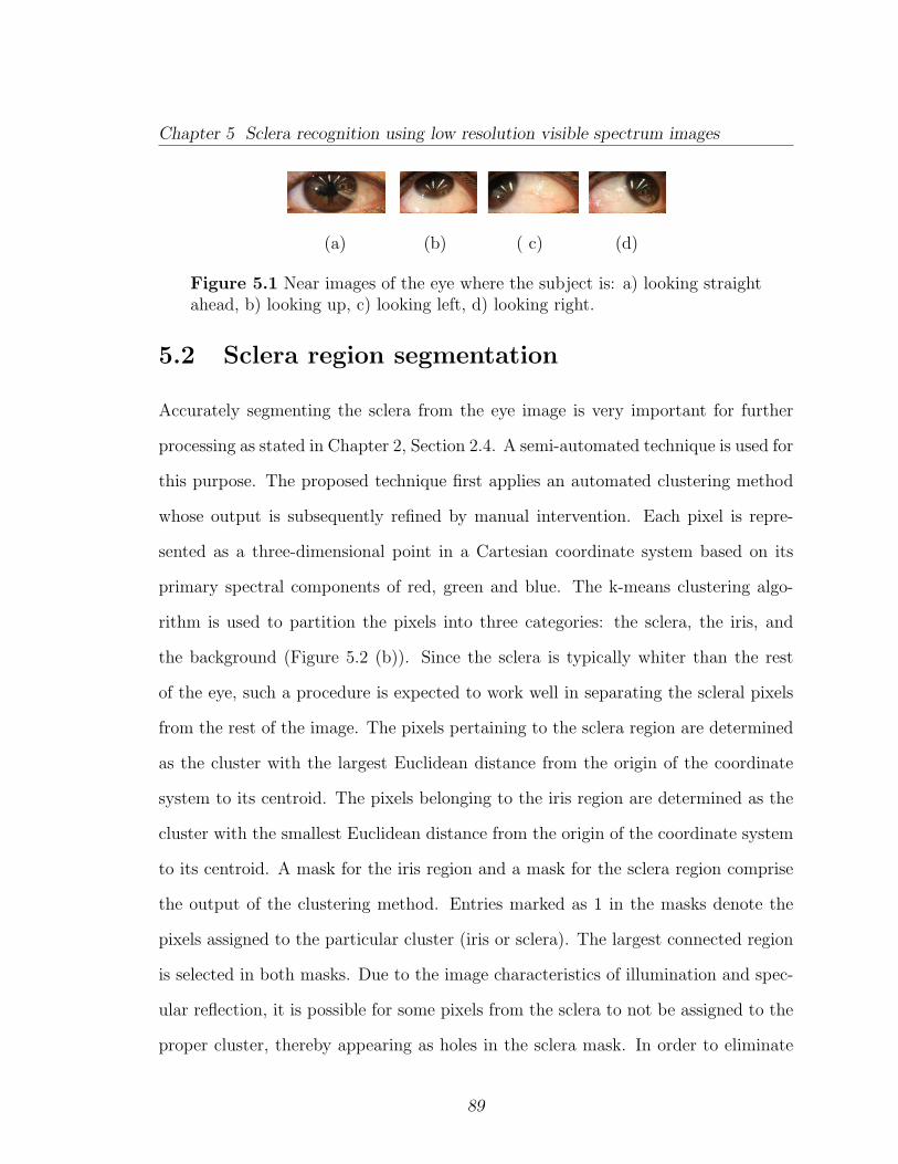
Chapter 5 Sclera recognition using low resolution visible spectrum images
(a) (b) ( c) (d)
Figure 5.1 Near images of the eye where the subject is: a) looking straightahead, b) looking up, c) looking left, d) looking right.
5.2 Sclera region segmentation
Accurately segmenting the sclera from the eye image is very important for further
processing as stated in Chapter 2, Section 2.4. A semi-automated technique is used for
this purpose. The proposed technique first applies an automated clustering method
whose output is subsequently refined by manual intervention. Each pixel is repre-
sented as a three-dimensional point in a Cartesian coordinate system based on its
primary spectral components of red, green and blue. The k-means clustering algo-
rithm is used to partition the pixels into three categories: the sclera, the iris, and
the background (Figure 5.2 (b)). Since the sclera is typically whiter than the rest
of the eye, such a procedure is expected to work well in separating the scleral pixels
from the rest of the image. The pixels pertaining to the sclera region are determined
as the cluster with the largest Euclidean distance from the origin of the coordinate
system to its centroid. The pixels belonging to the iris region are determined as the
cluster with the smallest Euclidean distance from the origin of the coordinate system
to its centroid. A mask for the iris region and a mask for the sclera region comprise
the output of the clustering method. Entries marked as 1 in the masks denote the
pixels assigned to the particular cluster (iris or sclera). The largest connected region
is selected in both masks. Due to the image characteristics of illumination and spec-
ular reflection, it is possible for some pixels from the sclera to not be assigned to the
proper cluster, thereby appearing as holes in the sclera mask. In order to eliminate
89
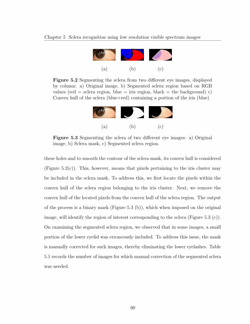
Chapter 5 Sclera recognition using low resolution visible spectrum images
Cluster Data
(a) (b) (c)
Figure 5.2 Segmenting the sclera from two different eye images, displayedby column: a) Original image, b) Segmented sclera region based on RGBvalues (red = sclera region, blue = iris region, black = the background) c)Convex hull of the sclera (blue+red) containing a portion of the iris (blue)
(a) (b) (c)
Figure 5.3 Segmenting the sclera of two different eye images: a) Originalimage, b) Sclera mask, c) Segmented sclera region.
these holes and to smooth the contour of the sclera mask, its convex hull is considered
(Figure 5.2(c)). This, however, means that pixels pertaining to the iris cluster may
be included in the sclera mask. To address this, we first locate the pixels within the
convex hull of the sclera region belonging to the iris cluster. Next, we remove the
convex hull of the located pixels from the convex hull of the sclera region. The output
of the process is a binary mask (Figure 5.3 (b)), which when imposed on the original
image, will identify the region of interest corresponding to the sclera (Figure 5.3 (c)).
On examining the segmented sclera region, we observed that in some images, a small
portion of the lower eyelid was erroneously included. To address this issue, the mask
is manually corrected for such images, thereby eliminating the lower eyelashes. Table
5.1 records the number of images for which manual correction of the segmented sclera
was needed.
90
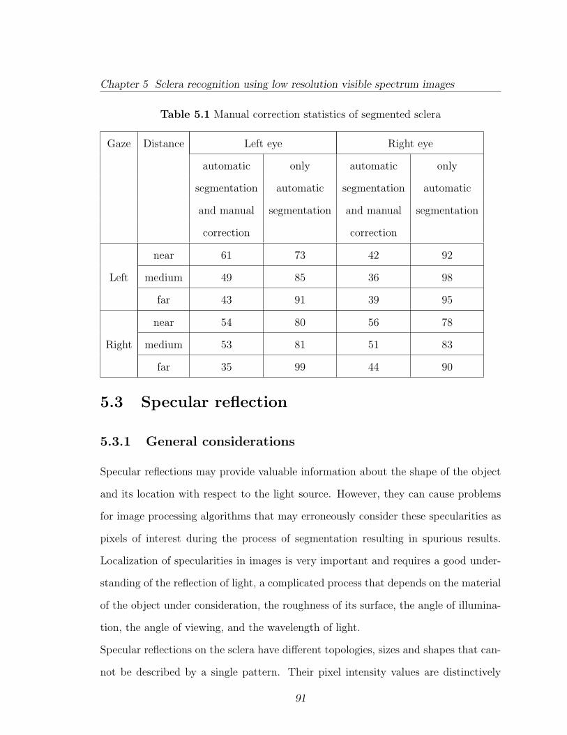
Chapter 5 Sclera recognition using low resolution visible spectrum images
Table 5.1 Manual correction statistics of segmented sclera
Gaze Distance Left eye Right eye
automatic only automatic only
segmentation automatic segmentation automatic
and manual segmentation and manual segmentation
correction correction
Left
near 61 73 42 92
medium 49 85 36 98
far 43 91 39 95
Right
near 54 80 56 78
medium 53 81 51 83
far 35 99 44 90
5.3 Specular reflection
5.3.1 General considerations
Specular reflections may provide valuable information about the shape of the object
and its location with respect to the light source. However, they can cause problems
for image processing algorithms that may erroneously consider these specularities as
pixels of interest during the process of segmentation resulting in spurious results.
Localization of specularities in images is very important and requires a good under-
standing of the reflection of light, a complicated process that depends on the material
of the object under consideration, the roughness of its surface, the angle of illumina-
tion, the angle of viewing, and the wavelength of light.
Specular reflections on the sclera have different topologies, sizes and shapes that can-
not be described by a single pattern. Their pixel intensity values are distinctively
91
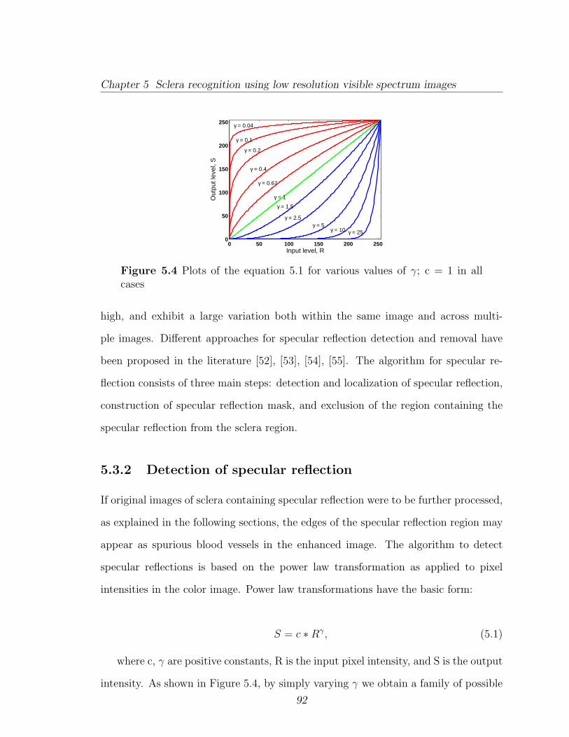
Chapter 5 Sclera recognition using low resolution visible spectrum images
0 50 100 150 200 2500
50
100
150
200
250
Input level, R
Out
put l
evel
, S
γ = 0.04
γ = 0.1
γ = 0.2
γ = 0.4
γ = 0.67
γ = 1
γ = 1.5
γ = 2.5γ = 5
γ = 10 γ = 25
Figure 5.4 Plots of the equation 5.1 for various values of γ; c = 1 in allcases
high, and exhibit a large variation both within the same image and across multi-
ple images. Different approaches for specular reflection detection and removal have
been proposed in the literature [52], [53], [54], [55]. The algorithm for specular re-
flection consists of three main steps: detection and localization of specular reflection,
construction of specular reflection mask, and exclusion of the region containing the
specular reflection from the sclera region.
5.3.2 Detection of specular reflection
If original images of sclera containing specular reflection were to be further processed,
as explained in the following sections, the edges of the specular reflection region may
appear as spurious blood vessels in the enhanced image. The algorithm to detect
specular reflections is based on the power law transformation as applied to pixel
intensities in the color image. Power law transformations have the basic form:
S = c ∗Rγ, (5.1)
where c, γ are positive constants, R is the input pixel intensity, and S is the output
intensity. As shown in Figure 5.4, by simply varying γ we obtain a family of possible
92

Chapter 5 Sclera recognition using low resolution visible spectrum images
transformation curves. For γ > 1, the power - law curves map a narrow range of light
input values into a wider range of output values. For γ < 1, the power - law curves
map a narrow range of dark input values into a wider range of output values. In order
to detect specularities, we consider γ an integer in the range [1, 10]. The detection of
the specular reflection is as follows.
1. Convert the RGB image to the HSI (hue, saturation, illumination) color space.
2. Consider the illumination component of the HSI space as the input image R in
equation 5.1.
3. Compute the output image S for different γ values using equation 5.1. Fig. 5.5
(a) displays results for gamma = 3.
4. Compute the histogram for each image S as seen in Fig. 5.5 (b).
5. Compute the filtered histogram for each image S using the moving average [1/3
1/3 1/3] filter as seen in Fig. 5.5 (c).
6. Compute the slope θ of the filtered histogram.
7. For the filtered histogram corresponding to each γ, find the first negative θ (θγ)
and its corresponding intensity value, Sγ, as a potential threshold value for
detecting specular reflection.
8. Examine the distribution of θγ as a function of γ to select γopt, γopt = arg max (|
θγ − θγ−1 |). Figure 5.6 shows γopt = 5 ; for near distance images, the threshold
to detect specular reflection is selected as the mean of all thresholds values
found for γ, 5 ≤ γ ≤ 10.
9. Use the threshold value found to obtain a binary mask for isolating specular re-
flection.
93
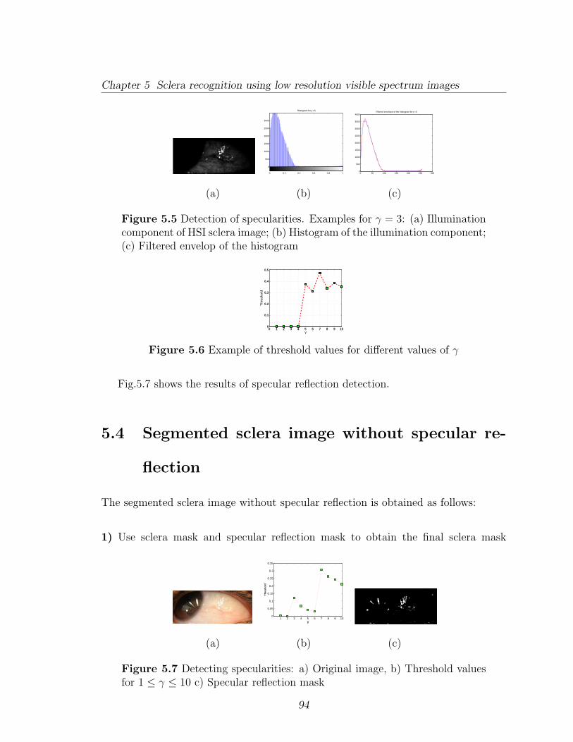
Chapter 5 Sclera recognition using low resolution visible spectrum images
0 0.2 0.4 0.6 0.8 1
0
500
1000
1500
2000
2500
3000
Histogram for γ =3
0 50 100 150 200 250 3000
500
1000
1500
2000
2500
3000
3500
4000Filtered envelope of the histogram for γ =3
(a) (b) (c)
Figure 5.5 Detection of specularities. Examples for γ = 3: (a) Illuminationcomponent of HSI sclera image; (b) Histogram of the illumination component;(c) Filtered envelop of the histogram
0 1 2 3 4 5 6 7 8 9 100
0.1
0.2
0.3
0.4
0.5
γ
Thr
esho
ld
Figure 5.6 Example of threshold values for different values of γ
Fig.5.7 shows the results of specular reflection detection.
5.4 Segmented sclera image without specular re-
flection
The segmented sclera image without specular reflection is obtained as follows:
1) Use sclera mask and specular reflection mask to obtain the final sclera mask
1 2 3 4 5 6 7 8 9 100
0.05
0.1
0.15
0.2
0.25
0.3
0.35
γ
Th
resh
old
(a) (b) (c)
Figure 5.7 Detecting specularities: a) Original image, b) Threshold valuesfor 1 ≤ γ ≤ 10 c) Specular reflection mask
94
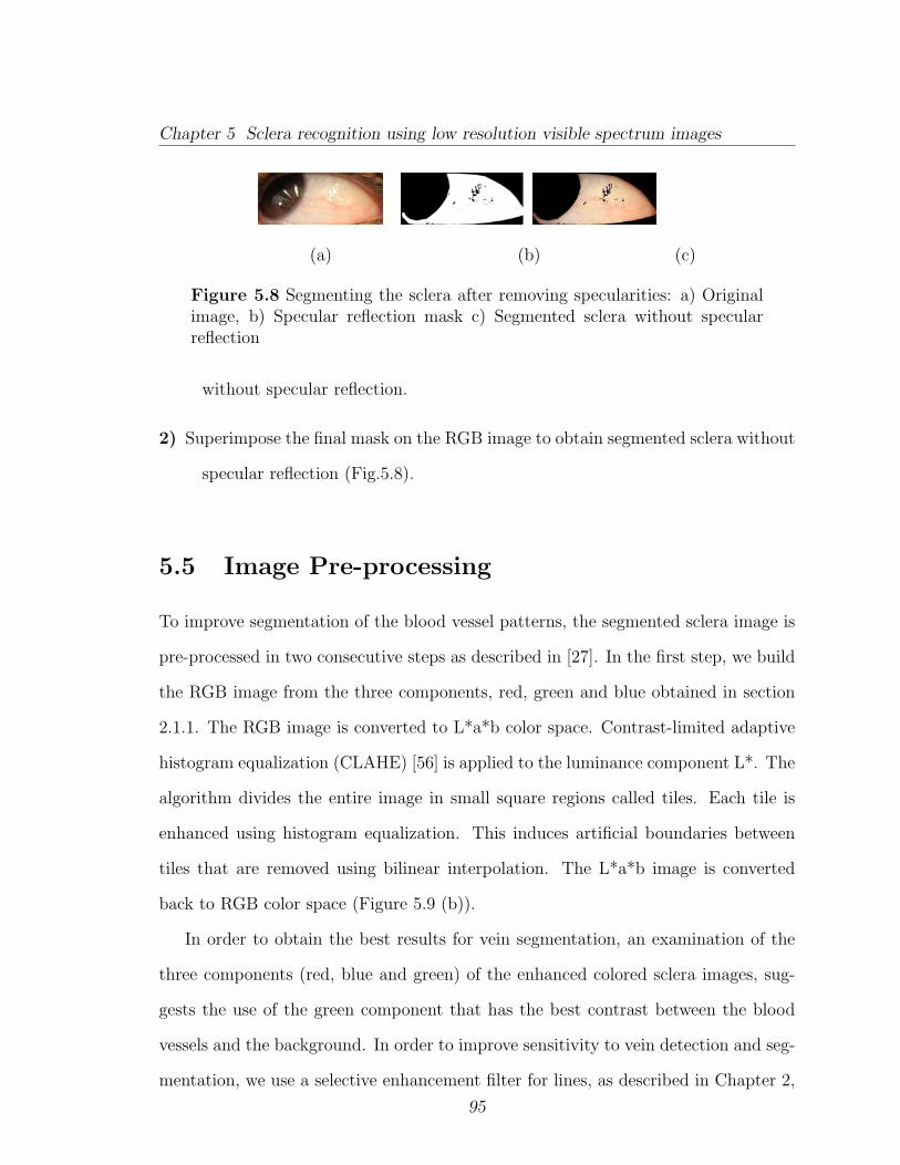
Chapter 5 Sclera recognition using low resolution visible spectrum images
(a) (b) (c)
Figure 5.8 Segmenting the sclera after removing specularities: a) Originalimage, b) Specular reflection mask c) Segmented sclera without specularreflection
without specular reflection.
2) Superimpose the final mask on the RGB image to obtain segmented sclera without
specular reflection (Fig.5.8).
5.5 Image Pre-processing
To improve segmentation of the blood vessel patterns, the segmented sclera image is
pre-processed in two consecutive steps as described in [27]. In the first step, we build
the RGB image from the three components, red, green and blue obtained in section
2.1.1. The RGB image is converted to L*a*b color space. Contrast-limited adaptive
histogram equalization (CLAHE) [56] is applied to the luminance component L*. The
algorithm divides the entire image in small square regions called tiles. Each tile is
enhanced using histogram equalization. This induces artificial boundaries between
tiles that are removed using bilinear interpolation. The L*a*b image is converted
back to RGB color space (Figure 5.9 (b)).
In order to obtain the best results for vein segmentation, an examination of the
three components (red, blue and green) of the enhanced colored sclera images, sug-
gests the use of the green component that has the best contrast between the blood
vessels and the background. In order to improve sensitivity to vein detection and seg-
mentation, we use a selective enhancement filter for lines, as described in Chapter 2,
95

Chapter 5 Sclera recognition using low resolution visible spectrum images
(a) (b)
Figure 5.9 Image Enhancement:(a) Original sclera vein image, (b) Enhancedsclera vein image.
Figure 5.10 Example of pre-processed sclera vein image.
Section 2.5. Results are displayed in Figure 5.10.
After enhancement, images are registered using the algorithm presented in Chap-
ter 2, Section 2.6.
5.6 Matching Results
The similarity between two sclera images is assessed using cross-correlation between
regions of the sclera that do not include the specular reflections from both images.
Results are displayed in Figure 5.11. In the case of low resolution, unconstrained
images, the initial analysis indicates that an EER of ∼ 25% has been obtained on
a subset of images belonging to the left-eye-looking-left, near-distance category. An
assessment of the results suggests that the large intra-class variation is caused by the
following factors: (a) the curved surface of the eye that cannot be modeled using a
linear surface; (b) the large range of viewing angles; (c) the glossy surface of the sclera
that reflects light; (d) eyelashes that obstruct the sclera region and can be incorrectly
perceived as vasculature patterns; and (e) the presence of less prominent veins that
can degrade performance.
96
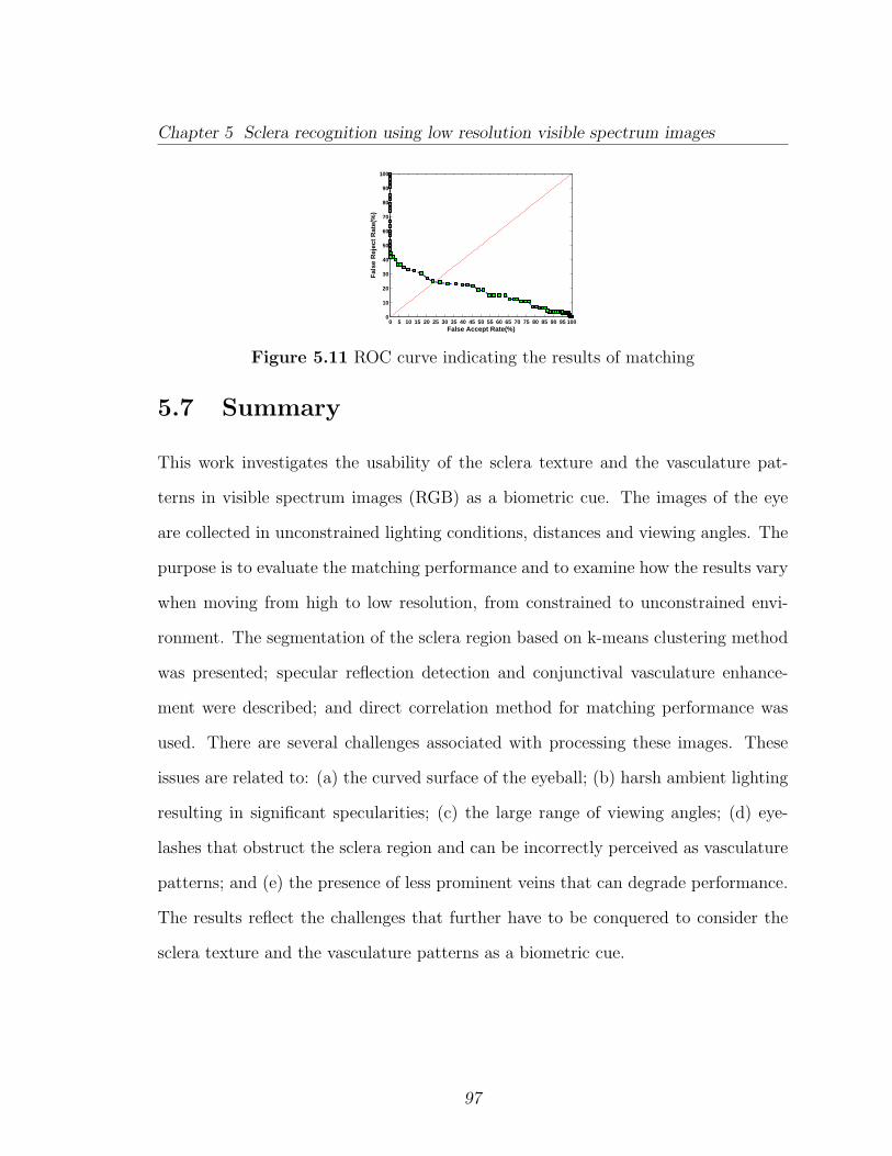
Chapter 5 Sclera recognition using low resolution visible spectrum images
0 5 10 15 20 25 30 35 40 45 50 55 60 65 70 75 80 85 90 95 1000
10
20
30
40
50
60
70
80
90
100
False Accept Rate(%)
Fal
se R
ejec
t R
ate(
%)
Figure 5.11 ROC curve indicating the results of matching
5.7 Summary
This work investigates the usability of the sclera texture and the vasculature pat-
terns in visible spectrum images (RGB) as a biometric cue. The images of the eye
are collected in unconstrained lighting conditions, distances and viewing angles. The
purpose is to evaluate the matching performance and to examine how the results vary
when moving from high to low resolution, from constrained to unconstrained envi-
ronment. The segmentation of the sclera region based on k-means clustering method
was presented; specular reflection detection and conjunctival vasculature enhance-
ment were described; and direct correlation method for matching performance was
used. There are several challenges associated with processing these images. These
issues are related to: (a) the curved surface of the eyeball; (b) harsh ambient lighting
resulting in significant specularities; (c) the large range of viewing angles; (d) eye-
lashes that obstruct the sclera region and can be incorrectly perceived as vasculature
patterns; and (e) the presence of less prominent veins that can degrade performance.
The results reflect the challenges that further have to be conquered to consider the
sclera texture and the vasculature patterns as a biometric cue.
97

Chapter 6
Discussions and Conclusions
Among different biometric modalities, iris recognition has gained popularity in the
last decade due to its reliability, accuracy, and stability over long periods of time.
However, it has been noted that when the gaze direction is non-frontal in regards to
the imaging device, the performance of iris recognition degrades considerably. The
idea of using the sclera surface as a biometric modality was developed to compensate
the loss of information in non-frontal images of the iris. There is an academic interest
in sclera biometrics as an individual and independent component of biometric science.
Based on the patent [24] approved in 2008, the work in this dissertation investigates
the novel use of the sclera texture and blood vessels seen on its surface as a biometric
cue. This new modality is presented as a potential part of the ocular biometric entity
that reunites all the biometric modalities related to the eye and its surrounding re-
gion. Iris patterns are better observed in the NIR spectrum, while the blood vessels
exposed on the sclera surface are better discerned in the visible spectrum. Therefore,
multispectral images of the eye are used to ensure that both the iris and the sclera
region are successfully imaged. A high resolution multispectral database consisting of
two different collections - the first of 103 subjects and the second of 31 subjects - was
98
Chapter 6 Discussions and Conclusions
assembled to initiate the research in this field. The images were collected within spe-
cific constraints that included stable lighting, consistent distance, and similar viewing
angles. The pre-processing and post-processing of the ocular images required image
denoising; specular reflection detection and removal; automatic segmentation of the
sclera, the iris, and the pupil;blood vessel enhancement; and image registration. To
evaluate and assess the performance of the sclera texture as a biometric modality,
first we had to find the feature extraction methods and matching algorithms that
better characterized this biometric. The study of the sclera texture as a biometric
modality was accomplished through four approaches.
1. The performance of sclera texture is evaluated by using three feature extraction
and matching schemes: SURF, a keypoint-based matching method; direct cor-
relation methods such as correlation, mutual information, normalized mutual
information, root mean square error, structural similarity index measure, and
ratio-image uniformity, such as pixel to pixel matching; and minutiae point
matching, which mark the locations of bifurcations of blood vessels visible on
the sclera region. The score level fusion of minutiae with each of the direct
correlation methods is evaluated using the simple sum rule, maximum rule, and
minimum rule (Chapter 3).
2. After establishing the potential use of sclera as a biometric cue, the matching
performance of the fusion of sclera patterns (scores obtained with SURF tech-
nique) with iris patterns (scores obtained with Hamming distance) is evaluated
by using three score level fusion rules: simple sum rule, maximum rule, and
minimum rule (Chapter 4).
3. The matching performance of the sclera texture as a potential biometric modality
is evaluated for data sets with intra-class variation. The methods used for
99
Chapter 6 Discussions and Conclusions
feature extraction and matching schemes are the ones used in the first approach.
The performance of the fusion of the sclera biometric (using SURF technique)
and the iris biometric (using Hamming distance) is also evaluated (Chapter 5).
4. The evaluation of sclera texture as a biometric in unconstrained, low resolution
visible spectrum images. (Chapter 6).
The first approach investigated the feasibility of using multispectral conjunctival
vasculature in an ocular biometric system. Due to its relative novelty as a research
topic, this paper mainly covers the challenges imposed when acquiring and processing
sclera images and should therefore be treated as a gateway to further exploration of
the sclera veins as a biometric modality. A new sclera segmentation method was pre-
sented and different feature extraction and matching techniques were used to represent
this biometric. The matching results using all the methods indicate lower values of
EER for left-eye-looking-left (L L) and right-eye-looking-right (R R) compared with
right-eye-looking-left (R L) and left-eye-looking-right (L R). This is because the fa-
cial features (such as the nose) partially obstruct the light directed to the left eye
when looking right and to the right eye when looking left. In such cases the EER
is improved using fusion methods. The best accuracy (EER < 0.8% for L L, R R,
and EER < 1.8% for L R, R L) is obtained when interest-point detection (SURF)
is used. This is because SURF utilizes the entire sclera region, including the vascu-
lature patterns; further it is not sensitive to small variations in the viewing angle,
affine deformations, and the color shades. Direct correlation measures also provide
good results, mainly when correlation (EER < 1.3% for L L, R R, and EER < 4.8%
for L R, R L) and normalized mutual information (EER < 1.7% for L L, R R, and
EER < 5.3% for L R, R L) are used. Like the SURF method, direct correlation
measures use the entire sclera surface including the conjunctival vasculature, but in
100
Chapter 6 Discussions and Conclusions
contrast are sensitive to changes in the viewing angle and illumination. Results could
be improved with a better blood vessel enhancement method. The minutiae based
method presents an EER in the range [9.5%, 12%] for both eyes and both gaze direc-
tions. The performance is greatly impacted by the presence of more or less prominent
veins, by the percentage of successfully segmented blood vessels and the accuracy with
which the centerline of the blood vessels is found. The perceived shape and tortuosity
of the blood vessels are influenced by the small changes in the viewing angle. This
method can be improved by accurately segmenting the blood vessels resulting in a
higher percentage of segmented blood vessels containing finer veins. The fusion of
direct correlation measure scores with minutiae scores is performed in an attempt to
boost the matching performance. In the case of left-eye-looking-right and right-eye-
looking-left, where the light that reaches the eye is obstructed by the facial structure
and the curvature of the eyeball, the EER is lowered when the sum rule is used for
fusing minutiae based scores with each of the direct correlation scores, except when
using mutual information and normalized mutual information.
The second approach investigated the benefits of combining the iris biometric with
the sclera biometric. The first approach demonstrated that SURF technique resulted
in the best recognition performance for scleral patterns. Therefore, this technique
was used to further combine the sclera patterns with iris patterns. Among differ-
ent evaluation techniques for iris biometric, Hamming distance is one of the most
popular. Three techniques were used to fuse the SURF scores with the Hamming dis-
tance scores: the simple sum rule, maximum rule, and minimum rule. As observed,
the combination of the two biometric modalities resulted in improved iris recognition
performance, especially when the simple sum rule or maximum rule was used. The
EER had the value of 0% for both eyes and both gaze directions, and there was no
overlap between the genuine and impostor distribution of scores. The performance of
101
Chapter 6 Discussions and Conclusions
iris recognition was also improved when using the minimum rule. The values of the
EER, which were obtained using Hamming distance, were between 0.45% and 3.5%.
After the fusion of the iris and the sclera patterns, the EER values were limited to
the interval 0.2% to 0.4%. The results suggested that iris recognition performance
would be improved by the fusion with sclera recognition.
The third approach investigated the potential of using the sclera patterns as a
biometric cue in the presence of intra-class variation. However, sclera recognition
exhibited the same performance with or without the presence of intra-class variation
when keypoint-based method SURF was used. The EER values were contained within
the interval 0.1% to 0.8% for left-eye-looking-left, right-eye-looking-right, and right-
eye-looking-left. Only the value of EER for the left-eye-looking-right was slightly
higher, at 2.5%. SURF technique is invariant to small changes in the viewing an-
gle. By comparison, the direct correlation techniques and minutiae points method
are not invariant to the changes in the viewing angle. Therefore, a decrease in the
performance of sclera recognition was observed when the variant methods were used.
The EER values for minutiae points were constrained to the interval 11.5% to 16%,
which were also higher values when compared with those from the Table 2.6. The
performance of iris recognition in this approach was more positive than when com-
pared with the values of EER obtained in the second approach. This is explained
by a better illumination of the eye and the focus of the camera on the iris region.
Similarly, the iris recognition performance for ocular images with intra-class variation
was increased as a result of the fusion of iris patterns with sclera patterns.
The fourth and the last approach investigated the usability of the sclera texture
and the vasculature patterns in visible spectrum images (RGB) as a biometric cue.
The images collected in an unconstrained environment exhibited a large range of
viewing angles, specular reflections of different sizes, topologies, and locations. The
102

Chapter 6 Discussions and Conclusions
correlation was used for matching performance. For near distance, left-eye-looking-
left, the EER is 25%. A future step is to address the challenges encountered when
acquiring and processing images of the sclera collected in unconstrained environment.
The following publications were generated as a consequence of this research:
1. S. Crihalmeanu, A. Ross,Multispectral Scleral Patterns for Ocular Biometric
Recognition, Pattern Recognition Letters, In press 2012, http://dx.doi.org./10.1016/j.patrec.2011.11.006
2. S. Crihalmeanu and A. Ross, On the Use of Multispectral Conjunctival Vascula-
ture as a Soft Biometric, WACV, Kona USA, January 2011
3. S. Tankasala, P.Doynov, R. Derakhshani, A. Ross and S. Crihalmeanu, Classifi-
cation of Conjunctival Vasculature using GLCM Features, ICIIP, Shimla India,
November 2011
4. S. Crihalmeanu, A. Ross and R. Derakhshani, Enhancement and Registration
Schemes for Matching Conjunctival Vasculature, ICB, Alghero Italy, June 2009
5. R. Derakhshani, A. Ross and S. Crihalmeanu, A new Biometric Modality Based
On Conjunctival Vasculature, ANNIE, Saint Louis USA, November 2006
6.1 Future work
The results obtained in the four approaches described in this dissertation demonstrate
the potential of using the sclera surface and the conjunctival vasculature for recog-
nition and reflect the challenges that further have to be conquered to consider the
sclera texture and the vasculature patterns as a biometric cue. The results suggest
that more work is needed in this area, such as evaluating the sclera in non-frontal
103
Chapter 6 Discussions and Conclusions
images of the eye using texture analysis techniques described in [57]: color texture
analysis, random texture analysis, hierarchical texture, etc. Another approach could
be the study of segmented blood vessels as open curves, their tortuosity and thickness
(more or less prominent blood vessels), and the changes that occur with an incon-
sistent viewing angle. The detection of the eyelashes may help improve the sclera
region segmentation. Other issues that may be addressed are related to lessening
the constrains of the environment; for example, by evaluating the sclera surface in
ocular images with the entire sclera exposed (wide open eye) or partially occluded
sclera region, and evaluating the matching performance of the sclera texture under
different lighting conditions and different viewing angles. The age of the subject and
the chemicals the eye has come in contact with both greatly influence the appear-
ance of the sclera texture. These changes may have a significant effect not only on
the matching performance, but also on the segmentation process. It is well known
that an improper segmentation will also influence the performance matching. Little
research for iris recognition using multispectral images is published. A more in depth
exploitation of the multispectral information may support a more accurate segmen-
tation of the iris and sclera region, and feature extraction and matching algorithms.
The answers to all these issues lead to the innovative idea of customizing imaging
systems for sclera. As for any other biometric system, a quality measure has to be
found in order to address the problem of failure to acquire.
In this dissertation the possibility of utilizing the scleral patterns in conjunction
with the iris for recognizing ocular images exhibiting non-frontal gaze directions was
established.
104
Appendix A
Methods for sclera patterns
matching. The ROC and the
distribution of scores. Data
Collection 1
105
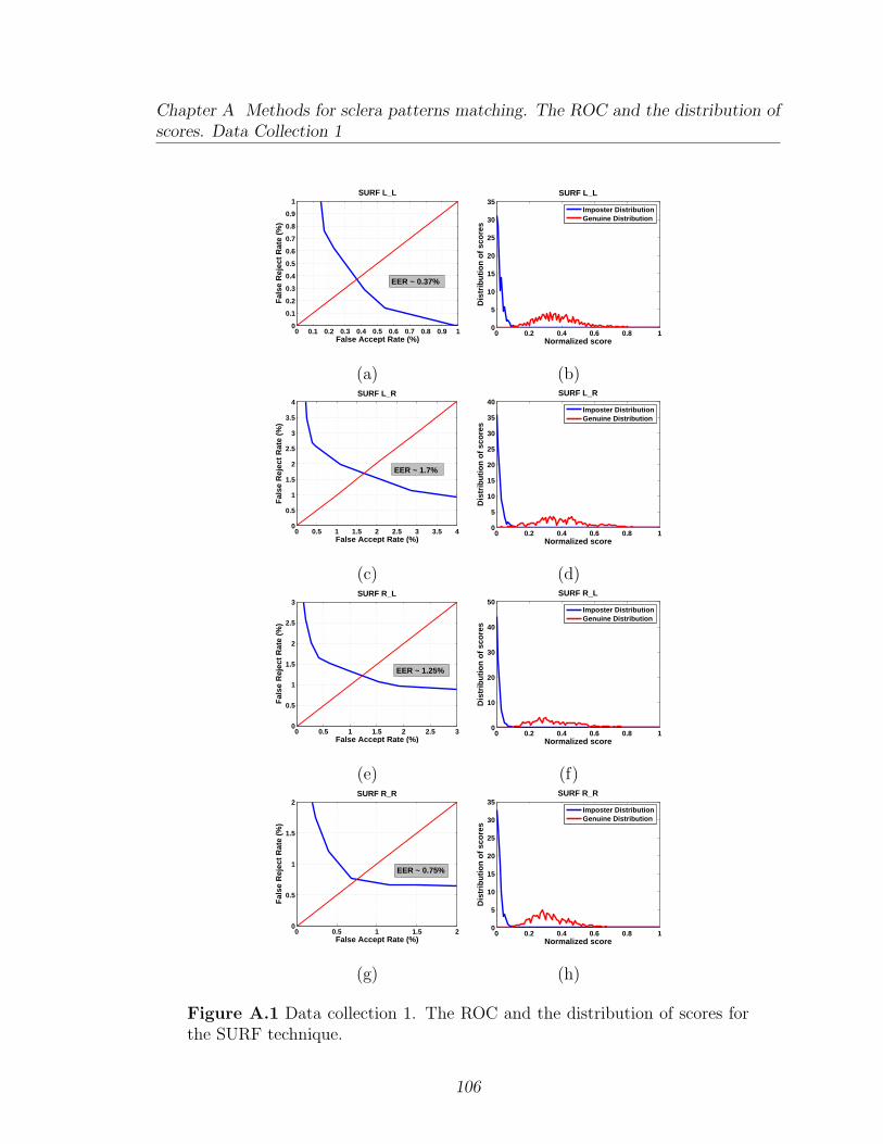
Chapter A Methods for sclera patterns matching. The ROC and the distribution ofscores. Data Collection 1
0 0.1 0.2 0.3 0.4 0.5 0.6 0.7 0.8 0.9 10
0.1
0.2
0.3
0.4
0.5
0.6
0.7
0.8
0.9
1SURF L_L
False Accept Rate (%)
Fal
se R
ejec
t R
ate
(%)
EER ~ 0.37%
0 0.2 0.4 0.6 0.8 10
5
10
15
20
25
30
35
Normalized score
Dis
trib
uti
on
of
sco
res
SURF L_L
Imposter DistributionGenuine Distribution
(a) (b)
0 0.5 1 1.5 2 2.5 3 3.5 40
0.5
1
1.5
2
2.5
3
3.5
4SURF L_R
False Accept Rate (%)
Fal
se R
ejec
t R
ate
(%)
EER ~ 1.7%
0 0.2 0.4 0.6 0.8 10
5
10
15
20
25
30
35
40
Normalized score
Dis
trib
uti
on
of
sco
res
SURF L_R
Imposter DistributionGenuine Distribution
(c) (d)
0 0.5 1 1.5 2 2.5 30
0.5
1
1.5
2
2.5
3SURF R_L
False Accept Rate (%)
Fal
se R
ejec
t R
ate
(%)
EER ~ 1.25%
0 0.2 0.4 0.6 0.8 10
10
20
30
40
50
Normalized score
Dis
trib
uti
on
of
sco
res
SURF R_L
Imposter DistributionGenuine Distribution
(e) (f)
0 0.5 1 1.5 20
0.5
1
1.5
2SURF R_R
False Accept Rate (%)
Fal
se R
ejec
t R
ate
(%)
EER ~ 0.75%
0 0.2 0.4 0.6 0.8 10
5
10
15
20
25
30
35
Normalized score
Dis
trib
uti
on
of
sco
res
SURF R_R
Imposter DistributionGenuine Distribution
(g) (h)
Figure A.1 Data collection 1. The ROC and the distribution of scores forthe SURF technique.
106
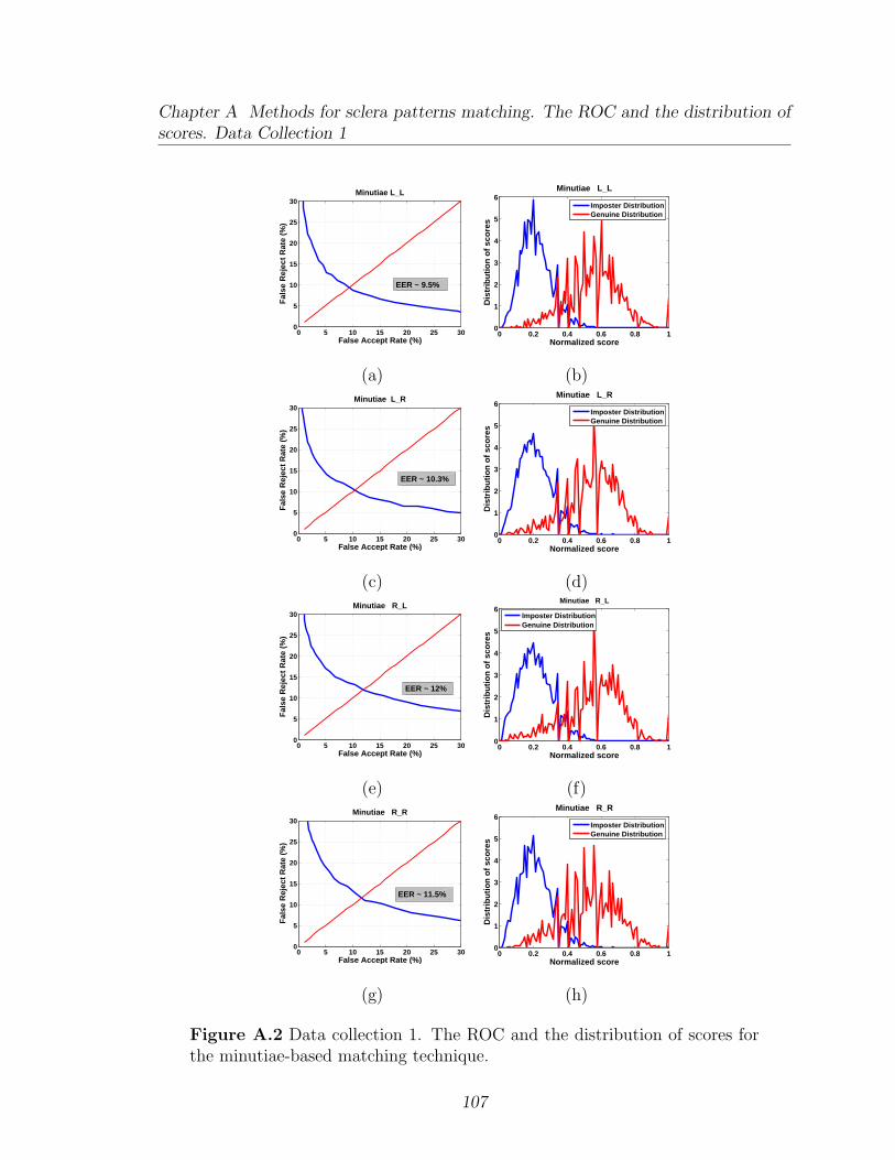
Chapter A Methods for sclera patterns matching. The ROC and the distribution ofscores. Data Collection 1
0 5 10 15 20 25 300
5
10
15
20
25
30
False Accept Rate (%)
Fal
se R
ejec
t R
ate
(%)
Minutiae L_L
EER ~ 9.5%
0 0.2 0.4 0.6 0.8 10
1
2
3
4
5
6
Normalized score
Dis
trib
uti
on
of
sco
res
Minutiae L_L
Imposter DistributionGenuine Distribution
(a) (b)
0 5 10 15 20 25 300
5
10
15
20
25
30
False Accept Rate (%)
Fal
se R
ejec
t R
ate
(%)
Minutiae L_R
EER ~ 10.3%
0 0.2 0.4 0.6 0.8 10
1
2
3
4
5
6
Normalized score
Dis
trib
uti
on
of
sco
res
Minutiae L_R
Imposter DistributionGenuine Distribution
(c) (d)
0 5 10 15 20 25 300
5
10
15
20
25
30
False Accept Rate (%)
Fal
se R
ejec
t R
ate
(%)
Minutiae R_L
EER ~ 12%
0 0.2 0.4 0.6 0.8 10
1
2
3
4
5
6
Normalized score
Dis
trib
uti
on
of
sco
res
Minutiae R_L
Imposter DistributionGenuine Distribution
(e) (f)
0 5 10 15 20 25 300
5
10
15
20
25
30
False Accept Rate (%)
Fal
se R
ejec
t R
ate
(%)
Minutiae R_R
EER ~ 11.5%
0 0.2 0.4 0.6 0.8 10
1
2
3
4
5
6
Normalized score
Dis
trib
uti
on
of
sco
res
Minutiae R_R
Imposter DistributionGenuine Distribution
(g) (h)
Figure A.2 Data collection 1. The ROC and the distribution of scores forthe minutiae-based matching technique.
107
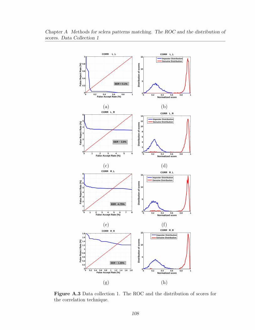
Chapter A Methods for sclera patterns matching. The ROC and the distribution ofscores. Data Collection 1
0 0.2 0.4 0.6 0.8 10
0.2
0.4
0.6
0.8
1
False Accept Rate (%)
Fal
se R
ejec
t R
ate
(%)
CORR L_L
EER = 0.1%
0 0.2 0.4 0.6 0.8 10
5
10
15
Normalized score
Dis
trib
uti
on
of
sco
res
CORR L_L
Imposter DistributionGenuine Distribution
(a) (b)
0 1 2 3 4 5 60
1
2
3
4
5
6
False Accept Rate (%)
Fal
se R
ejec
t R
ate
(%)
CORR L_R
EER ~ 3.5%
0 0.2 0.4 0.6 0.8 10
2
4
6
8
10
12
14
Normalized score
Dis
trib
uti
on
of
sco
res
CORR L_R
Imposter DistributionGenuine Distribution
(c) (d)
0 1 2 3 4 5 6 7 80
1
2
3
4
5
6
7
8
False Accept Rate (%)
Fal
se R
ejec
t R
ate
(%)
CORR R_L
EER ~4.75%
0 0.2 0.4 0.6 0.8 10
5
10
15
Normalized score
Dis
trib
uti
on
of
sco
res
CORR R_L
Imposter DistributionGenuine Distribution
(e) (f)
0 0.2 0.4 0.6 0.8 1 1.2 1.4 1.6 1.80
0.2
0.4
0.6
0.8
1
1.2
1.4
1.6
1.8
False Accept Rate (%)
Fal
se R
ejec
t R
ate
(%)
CORR R_R
EER ~ 1.25%
0 0.2 0.4 0.6 0.8 10
5
10
15
Normalized score
Dis
trib
uti
on
of
sco
res
CORR R_R
Imposter DistributionGenuine Distribution
(g) (h)
Figure A.3 Data collection 1. The ROC and the distribution of scores forthe correlation technique.
108
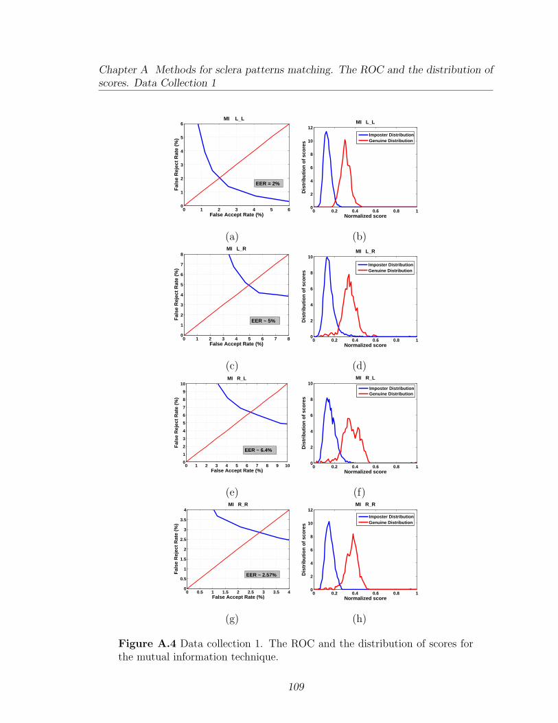
Chapter A Methods for sclera patterns matching. The ROC and the distribution ofscores. Data Collection 1
0 1 2 3 4 5 60
1
2
3
4
5
6
False Accept Rate (%)
Fal
se R
ejec
t R
ate
(%)
MI L_L
EER = 2%
0 0.2 0.4 0.6 0.8 10
2
4
6
8
10
12
Normalized score
Dis
trib
uti
on
of
sco
res
MI L_L
Imposter DistributionGenuine Distribution
(a) (b)
0 1 2 3 4 5 6 7 80
1
2
3
4
5
6
7
8
False Accept Rate (%)
Fal
se R
ejec
t R
ate
(%)
MI L_R
EER ~ 5%
0 0.2 0.4 0.6 0.8 10
2
4
6
8
10
Normalized score
Dis
trib
uti
on
of
sco
res
MI L_R
Imposter DistributionGenuine Distribution
(c) (d)
0 1 2 3 4 5 6 7 8 9 100
1
2
3
4
5
6
7
8
9
10
False Accept Rate (%)
Fal
se R
ejec
t R
ate
(%)
MI R_L
EER ~ 6.4%
0 0.2 0.4 0.6 0.8 10
2
4
6
8
10
Normalized score
Dis
trib
uti
on
of
sco
res
MI R_L
Imposter DistributionGenuine Distribution
(e) (f)
0 0.5 1 1.5 2 2.5 3 3.5 40
0.5
1
1.5
2
2.5
3
3.5
4
False Accept Rate (%)
Fal
se R
ejec
t R
ate
(%)
MI R_R
EER ~ 2.57%
0 0.2 0.4 0.6 0.8 10
2
4
6
8
10
12
Normalized score
Dis
trib
uti
on
of
sco
res
MI R_R
Imposter DistributionGenuine Distribution
(g) (h)
Figure A.4 Data collection 1. The ROC and the distribution of scores forthe mutual information technique.
109
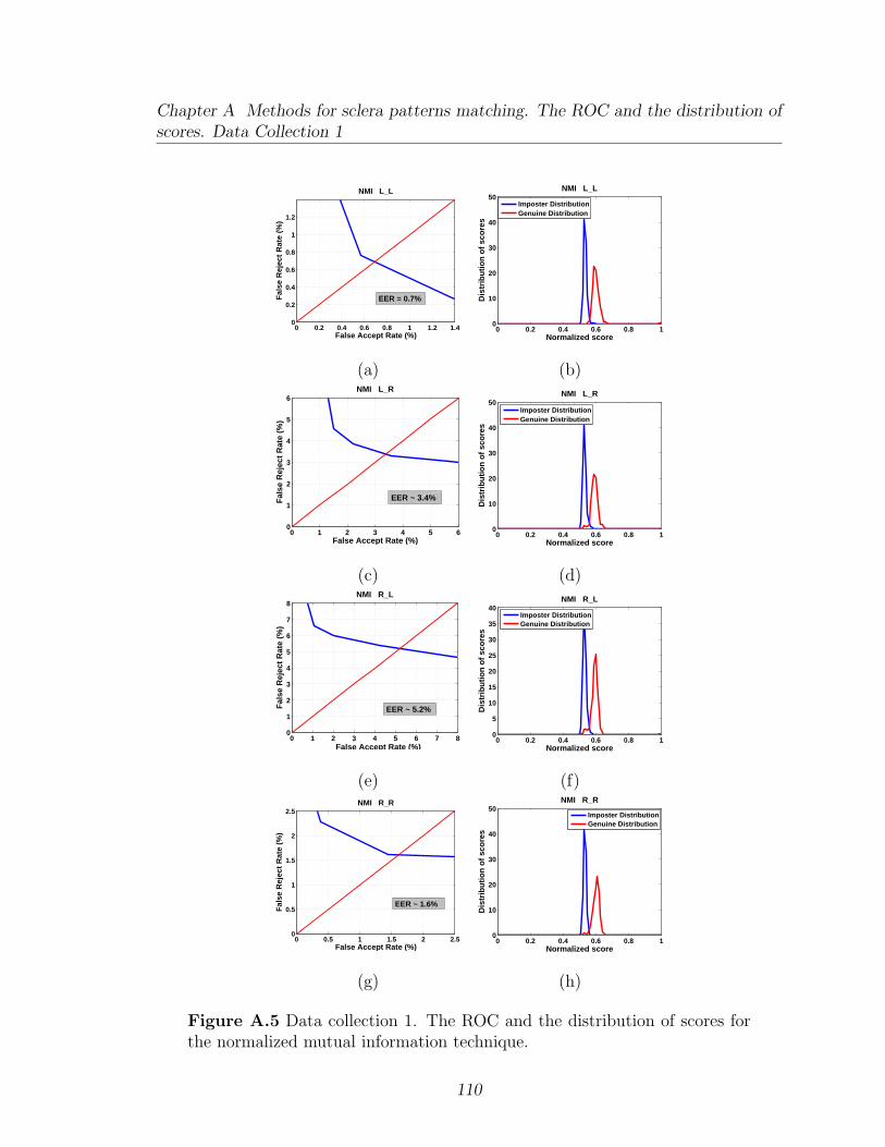
Chapter A Methods for sclera patterns matching. The ROC and the distribution ofscores. Data Collection 1
0 0.2 0.4 0.6 0.8 1 1.2 1.40
0.2
0.4
0.6
0.8
1
1.2
False Accept Rate (%)
Fal
se R
ejec
t R
ate
(%)
NMI L_L
EER = 0.7%
0 0.2 0.4 0.6 0.8 10
10
20
30
40
50
Normalized score
Dis
trib
uti
on
of
sco
res
NMI L_L
Imposter DistributionGenuine Distribution
(a) (b)
0 1 2 3 4 5 60
1
2
3
4
5
6
False Accept Rate (%)
Fal
se R
ejec
t R
ate
(%)
NMI L_R
EER ~ 3.4%
0 0.2 0.4 0.6 0.8 10
10
20
30
40
50
Normalized score
Dis
trib
uti
on
of
sco
res
NMI L_R
Imposter DistributionGenuine Distribution
(c) (d)
0 1 2 3 4 5 6 7 80
1
2
3
4
5
6
7
8
False Accept Rate (%)
Fal
se R
ejec
t R
ate
(%)
NMI R_L
EER ~ 5.2%
0 0.2 0.4 0.6 0.8 10
5
10
15
20
25
30
35
40
Normalized score
Dis
trib
uti
on
of
sco
res
NMI R_L
Imposter DistributionGenuine Distribution
(e) (f)
0 0.5 1 1.5 2 2.50
0.5
1
1.5
2
2.5
False Accept Rate (%)
Fal
se R
ejec
t R
ate
(%)
NMI R_R
EER ~ 1.6%
0 0.2 0.4 0.6 0.8 10
10
20
30
40
50
Normalized score
Dis
trib
uti
on
of
sco
res
NMI R_R
Imposter DistributionGenuine Distribution
(g) (h)
Figure A.5 Data collection 1. The ROC and the distribution of scores forthe normalized mutual information technique.
110
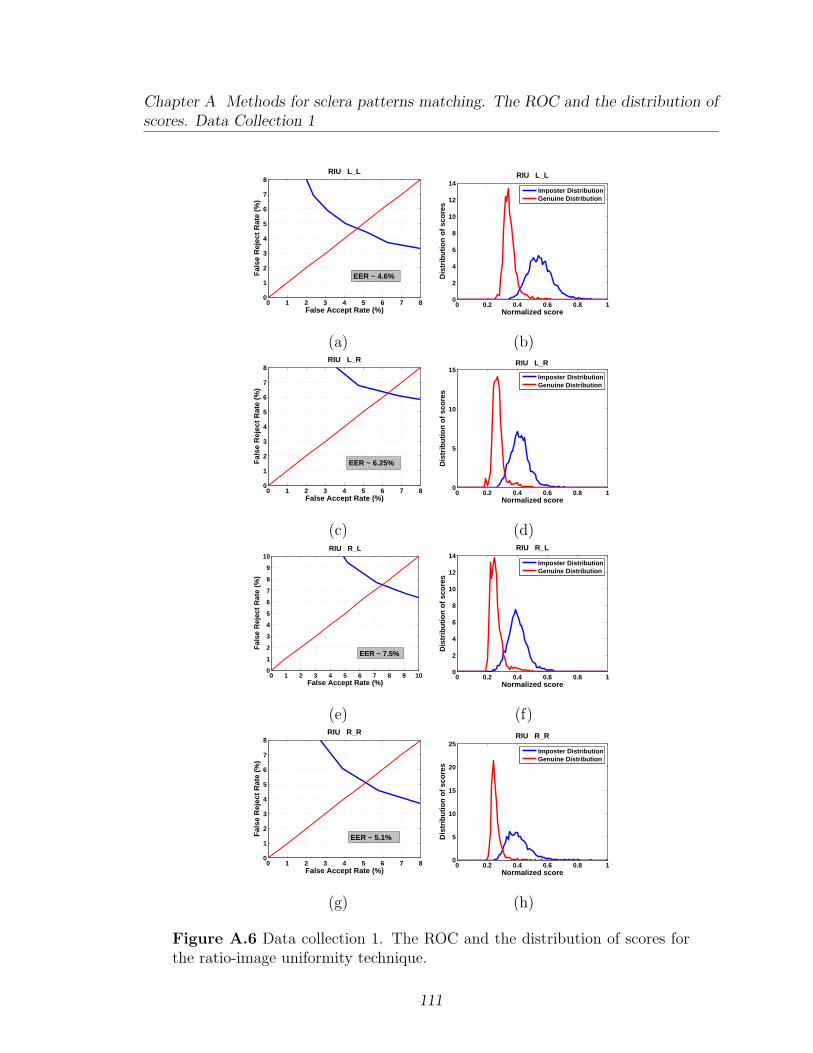
Chapter A Methods for sclera patterns matching. The ROC and the distribution ofscores. Data Collection 1
0 1 2 3 4 5 6 7 80
1
2
3
4
5
6
7
8
False Accept Rate (%)
Fal
se R
ejec
t R
ate
(%)
RIU L_L
EER ~ 4.6%
0 0.2 0.4 0.6 0.8 10
2
4
6
8
10
12
14
Normalized score
Dis
trib
uti
on
of
sco
res
RIU L_L
Imposter DistributionGenuine Distribution
(a) (b)
0 1 2 3 4 5 6 7 80
1
2
3
4
5
6
7
8
False Accept Rate (%)
Fal
se R
ejec
t R
ate
(%)
RIU L_R
EER ~ 6.25%
0 0.2 0.4 0.6 0.8 10
5
10
15
Normalized score
Dis
trib
uti
on
of
sco
res
RIU L_R
Imposter DistributionGenuine Distribution
(c) (d)
0 1 2 3 4 5 6 7 8 9 100
1
2
3
4
5
6
7
8
9
10
False Accept Rate (%)
Fal
se R
ejec
t R
ate
(%)
RIU R_L
EER ~ 7.5%
0 0.2 0.4 0.6 0.8 10
2
4
6
8
10
12
14
Normalized score
Dis
trib
uti
on
of
sco
res
RIU R_L
Imposter DistributionGenuine Distribution
(e) (f)
0 1 2 3 4 5 6 7 80
1
2
3
4
5
6
7
8
False Accept Rate (%)
Fal
se R
ejec
t R
ate
(%)
RIU R_R
EER ~ 5.1%
0 0.2 0.4 0.6 0.8 10
5
10
15
20
25
Normalized score
Dis
trib
uti
on
of
sco
res
RIU R_R
Imposter DistributionGenuine Distribution
(g) (h)
Figure A.6 Data collection 1. The ROC and the distribution of scores forthe ratio-image uniformity technique.
111
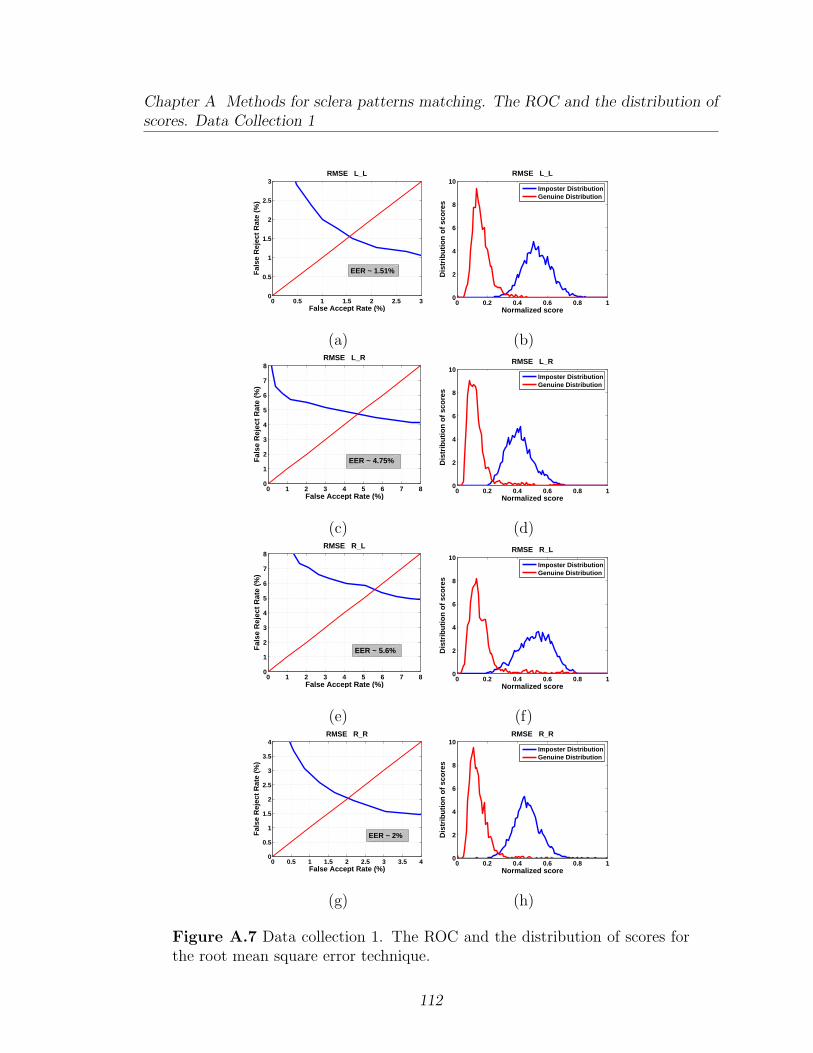
Chapter A Methods for sclera patterns matching. The ROC and the distribution ofscores. Data Collection 1
0 0.5 1 1.5 2 2.5 30
0.5
1
1.5
2
2.5
3
False Accept Rate (%)
Fal
se R
ejec
t R
ate
(%)
RMSE L_L
EER ~ 1.51%
0 0.2 0.4 0.6 0.8 10
2
4
6
8
10
Normalized score
Dis
trib
uti
on
of
sco
res
RMSE L_L
Imposter DistributionGenuine Distribution
(a) (b)
0 1 2 3 4 5 6 7 80
1
2
3
4
5
6
7
8
False Accept Rate (%)
Fal
se R
ejec
t R
ate
(%)
RMSE L_R
EER ~ 4.75%
0 0.2 0.4 0.6 0.8 10
2
4
6
8
10
Normalized score
Dis
trib
uti
on
of
sco
res
RMSE L_R
Imposter DistributionGenuine Distribution
(c) (d)
0 1 2 3 4 5 6 7 80
1
2
3
4
5
6
7
8
False Accept Rate (%)
Fal
se R
ejec
t R
ate
(%)
RMSE R_L
EER ~ 5.6%
0 0.2 0.4 0.6 0.8 10
2
4
6
8
10
Normalized score
Dis
trib
uti
on
of
sco
res
RMSE R_L
Imposter DistributionGenuine Distribution
(e) (f)
0 0.5 1 1.5 2 2.5 3 3.5 40
0.5
1
1.5
2
2.5
3
3.5
4
False Accept Rate (%)
Fal
se R
ejec
t R
ate
(%)
RMSE R_R
EER ~ 2%
0 0.2 0.4 0.6 0.8 10
2
4
6
8
10
Normalized score
Dis
trib
uti
on
of
sco
res
RMSE R_R
Imposter DistributionGenuine Distribution
(g) (h)
Figure A.7 Data collection 1. The ROC and the distribution of scores forthe root mean square error technique.
112
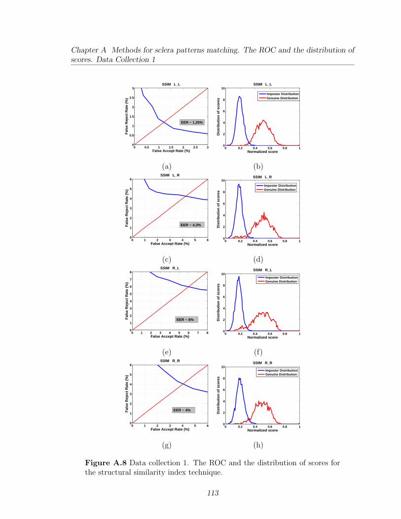
Chapter A Methods for sclera patterns matching. The ROC and the distribution ofscores. Data Collection 1
0 0.5 1 1.5 2 2.5 30
0.5
1
1.5
2
2.5
3
False Accept Rate (%)
Fal
se R
ejec
t R
ate
(%)
SSIM L_L
EER ~ 1.25%
0 0.2 0.4 0.6 0.8 10
2
4
6
8
10
Normalized score
Dis
trib
uti
on
of
sco
res
SSIM L_L
Imposter DistributionGenuine Distribution
(a) (b)
0 1 2 3 4 5 60
1
2
3
4
5
6
False Accept Rate (%)
Fal
se R
ejec
t R
ate
(%)
SSIM L_R
EER ~ 4.3%
0 0.2 0.4 0.6 0.8 10
2
4
6
8
10
Normalized score
Dis
trib
uti
on
of
sco
res
SSIM L_R
Imposter DistributionGenuine Distribution
(c) (d)
0 1 2 3 4 5 6 7 80
1
2
3
4
5
6
7
8
False Accept Rate (%)
Fal
se R
ejec
t R
ate
(%)
SSIM R_L
EER ~ 6%
0 0.2 0.4 0.6 0.8 10
2
4
6
8
10
Normalized score
Dis
trib
uti
on
of
sco
res
SSIM R_L
Imposter DistributionGenuine Distribution
(e) (f)
0 1 2 3 4 5 60
1
2
3
4
5
6
False Accept Rate (%)
Fal
se R
ejec
t R
ate
(%)
SSIM R_R
EER ~ 4%
0 0.2 0.4 0.6 0.8 10
2
4
6
8
10
Normalized score
Dis
trib
uti
on
of
sco
res
SSIM R_R
Imposter DistributionGenuine Distribution
(g) (h)
Figure A.8 Data collection 1. The ROC and the distribution of scores forthe structural similarity index technique.
113
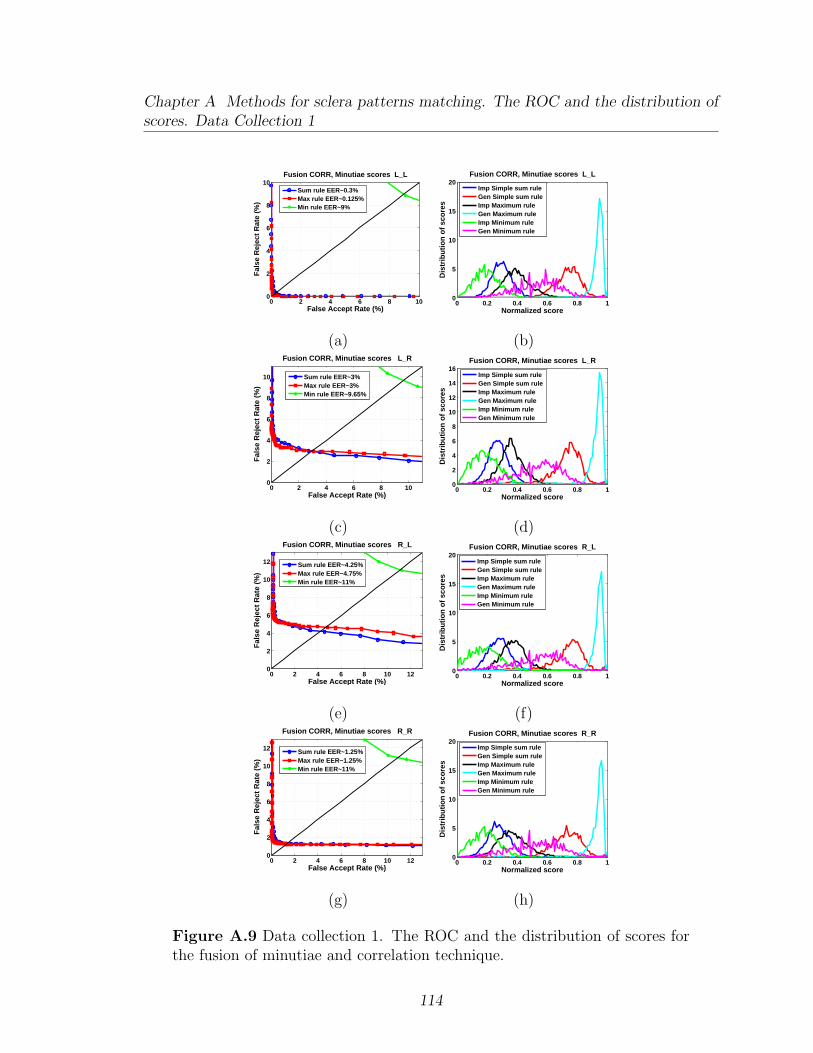
Chapter A Methods for sclera patterns matching. The ROC and the distribution ofscores. Data Collection 1
0 2 4 6 8 100
2
4
6
8
10Fusion CORR, Minutiae scores L_L
False Accept Rate (%)
Fal
se R
ejec
t R
ate
(%)
Sum rule EER~0.3%Max rule EER~0.125%Min rule EER~9%
0 0.2 0.4 0.6 0.8 10
5
10
15
20
Normalized score
Dis
trib
uti
on
of
sco
res
Fusion CORR, Minutiae scores L_L
Imp Simple sum ruleGen Simple sum ruleImp Maximum ruleGen Maximum ruleImp Minimum ruleGen Minimum rule
(a) (b)
0 2 4 6 8 100
2
4
6
8
10
Fusion CORR, Minutiae scores L_R
False Accept Rate (%)
Fal
se R
ejec
t R
ate
(%)
Sum rule EER~3%Max rule EER~3%Min rule EER~9.65%
0 0.2 0.4 0.6 0.8 10
2
4
6
8
10
12
14
16
Normalized score
Dis
trib
uti
on
of
sco
res
Fusion CORR, Minutiae scores L_R
Imp Simple sum ruleGen Simple sum ruleImp Maximum ruleGen Maximum ruleImp Minimum ruleGen Minimum rule
(c) (d)
0 2 4 6 8 10 120
2
4
6
8
10
12
Fusion CORR, Minutiae scores R_L
False Accept Rate (%)
Fal
se R
ejec
t R
ate
(%)
Sum rule EER~4.25%Max rule EER~4.75%Min rule EER~11%
0 0.2 0.4 0.6 0.8 10
5
10
15
20
Normalized score
Dis
trib
uti
on
of
sco
res
Fusion CORR, Minutiae scores R_L
Imp Simple sum ruleGen Simple sum ruleImp Maximum ruleGen Maximum ruleImp Minimum ruleGen Minimum rule
(e) (f)
0 2 4 6 8 10 120
2
4
6
8
10
12
Fusion CORR, Minutiae scores R_R
False Accept Rate (%)
Fal
se R
ejec
t R
ate
(%)
Sum rule EER~1.25%Max rule EER~1.25%Min rule EER~11%
0 0.2 0.4 0.6 0.8 10
5
10
15
20
Normalized score
Dis
trib
uti
on
of
sco
res
Fusion CORR, Minutiae scores R_R
Imp Simple sum ruleGen Simple sum ruleImp Maximum ruleGen Maximum ruleImp Minimum ruleGen Minimum rule
(g) (h)
Figure A.9 Data collection 1. The ROC and the distribution of scores forthe fusion of minutiae and correlation technique.
114
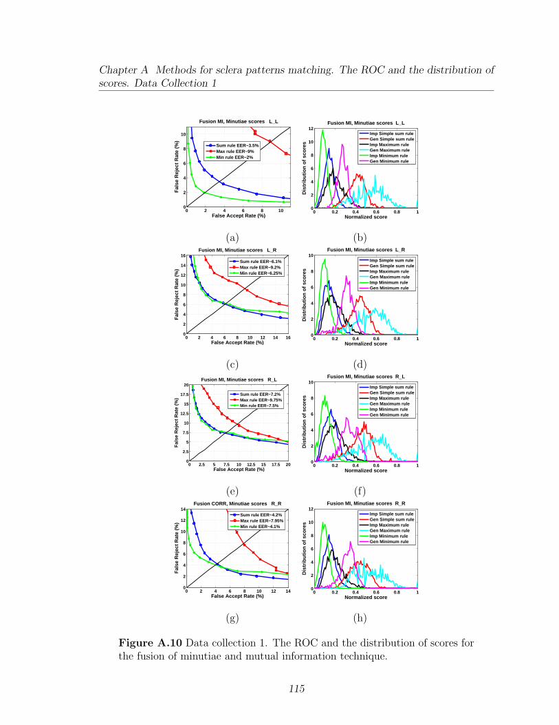
Chapter A Methods for sclera patterns matching. The ROC and the distribution ofscores. Data Collection 1
0 2 4 6 8 100
2
4
6
8
10
Fusion MI, Minutiae scores L_L
False Accept Rate (%)
Fal
se R
ejec
t R
ate
(%)
Sum rule EER~3.5%Max rule EER~9%Min rule EER~2%
0 0.2 0.4 0.6 0.8 10
2
4
6
8
10
12
Normalized score
Dis
trib
uti
on
of
sco
res
Fusion MI, Minutiae scores L_L
Imp Simple sum ruleGen Simple sum ruleImp Maximum ruleGen Maximum ruleImp Minimum ruleGen Minimum rule
(a) (b)
0 2 4 6 8 10 12 14 160
2
4
6
8
10
12
14
16Fusion MI, Minutiae scores L_R
False Accept Rate (%)
Fal
se R
ejec
t R
ate
(%)
Sum rule EER~6.1%Max rule EER~9.2%Min rule EER~6.25%
0 0.2 0.4 0.6 0.8 10
2
4
6
8
10
Normalized score
Dis
trib
uti
on
of
sco
res
Fusion MI, Minutiae scores L_R
Imp Simple sum ruleGen Simple sum ruleImp Maximum ruleGen Maximum ruleImp Minimum ruleGen Minimum rule
(c) (d)
0 2.5 5 7.5 10 12.5 15 17.5 200
2.5
5
7.5
10
12.5
15
17.5
20Fusion MI, Minutiae scores R_L
False Accept Rate (%)
Fal
se R
ejec
t R
ate
(%)
Sum rule EER~7.2%Max rule EER~9.75%Min rule EER~7.5%
0 0.2 0.4 0.6 0.8 10
2
4
6
8
10
Normalized score
Dis
trib
uti
on
of
sco
res
Fusion MI, Minutiae scores R_L
Imp Simple sum ruleGen Simple sum ruleImp Maximum ruleGen Maximum ruleImp Minimum ruleGen Minimum rule
(e) (f)
0 2 4 6 8 10 12 140
2
4
6
8
10
12
14Fusion CORR, Minutiae scores R_R
False Accept Rate (%)
Fal
se R
ejec
t R
ate
(%)
Sum rule EER~4.2%Max rule EER~7.95%Min rule EER~4.1%
0 0.2 0.4 0.6 0.8 10
2
4
6
8
10
12
Normalized score
Dis
trib
uti
on
of
sco
res
Fusion MI, Minutiae scores R_R
Imp Simple sum ruleGen Simple sum ruleImp Maximum ruleGen Maximum ruleImp Minimum ruleGen Minimum rule
(g) (h)
Figure A.10 Data collection 1. The ROC and the distribution of scores forthe fusion of minutiae and mutual information technique.
115
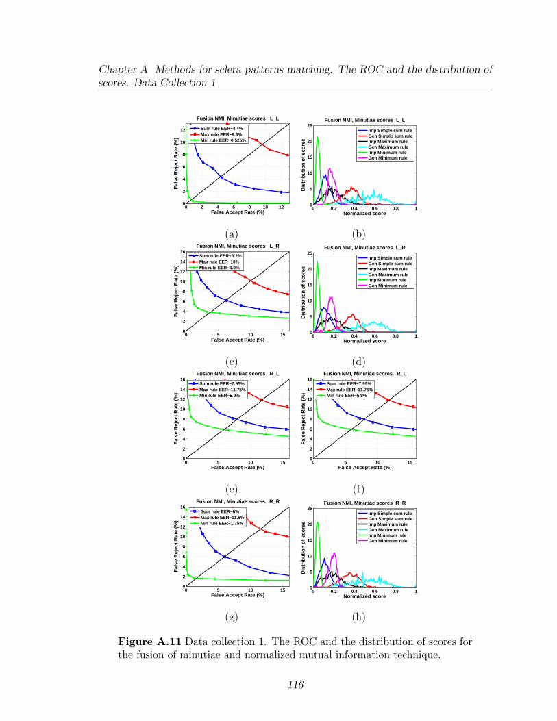
Chapter A Methods for sclera patterns matching. The ROC and the distribution ofscores. Data Collection 1
0 2 4 6 8 10 120
2
4
6
8
10
12
Fusion NMI, Minutiae scores L_L
False Accept Rate (%)
Fal
se R
ejec
t R
ate
(%)
Sum rule EER~4.4%Max rule EER~9.6%Min rule EER~0.525%
0 0.2 0.4 0.6 0.8 10
5
10
15
20
25
Normalized score
Dis
trib
uti
on
of
sco
res
Fusion NMI, Minutiae scores L_L
Imp Simple sum ruleGen Simple sum ruleImp Maximum ruleGen Maximum ruleImp Minimum ruleGen Minimum rule
(a) (b)
0 5 10 150
2
4
6
8
10
12
14
16Fusion NMI, Minutiae scores L_R
False Accept Rate (%)
Fal
se R
ejec
t R
ate
(%)
Sum rule EER~6.2%Max rule EER~10%Min rule EER~3.9%
0 0.2 0.4 0.6 0.8 10
5
10
15
20
25
Normalized score
Dis
trib
uti
on
of
sco
res
Fusion NMI, Minutiae scores L_R
Imp Simple sum ruleGen Simple sum ruleImp Maximum ruleGen Maximum ruleImp Minimum ruleGen Minimum rule
(c) (d)
0 5 10 150
2
4
6
8
10
12
14
16Fusion NMI, Minutiae scores R_L
False Accept Rate (%)
Fal
se R
ejec
t R
ate
(%)
Sum rule EER~7.95%Max rule EER~11.75%Min rule EER~5.9%
0 5 10 150
2
4
6
8
10
12
14
16Fusion NMI, Minutiae scores R_L
False Accept Rate (%)
Fal
se R
ejec
t R
ate
(%)
Sum rule EER~7.95%Max rule EER~11.75%Min rule EER~5.9%
(e) (f)
0 5 10 150
2
4
6
8
10
12
14
16Fusion NMI, Minutiae scores R_R
False Accept Rate (%)
Fal
se R
ejec
t R
ate
(%)
Sum rule EER~6%Max rule EER~11.5%Min rule EER~1.75%
0 0.2 0.4 0.6 0.8 10
5
10
15
20
25
Normalized score
Dis
trib
uti
on
of
sco
res
Fusion NMI, Minutiae scores R_R
Imp Simple sum ruleGen Simple sum ruleImp Maximum ruleGen Maximum ruleImp Minimum ruleGen Minimum rule
(g) (h)
Figure A.11 Data collection 1. The ROC and the distribution of scores forthe fusion of minutiae and normalized mutual information technique.
116
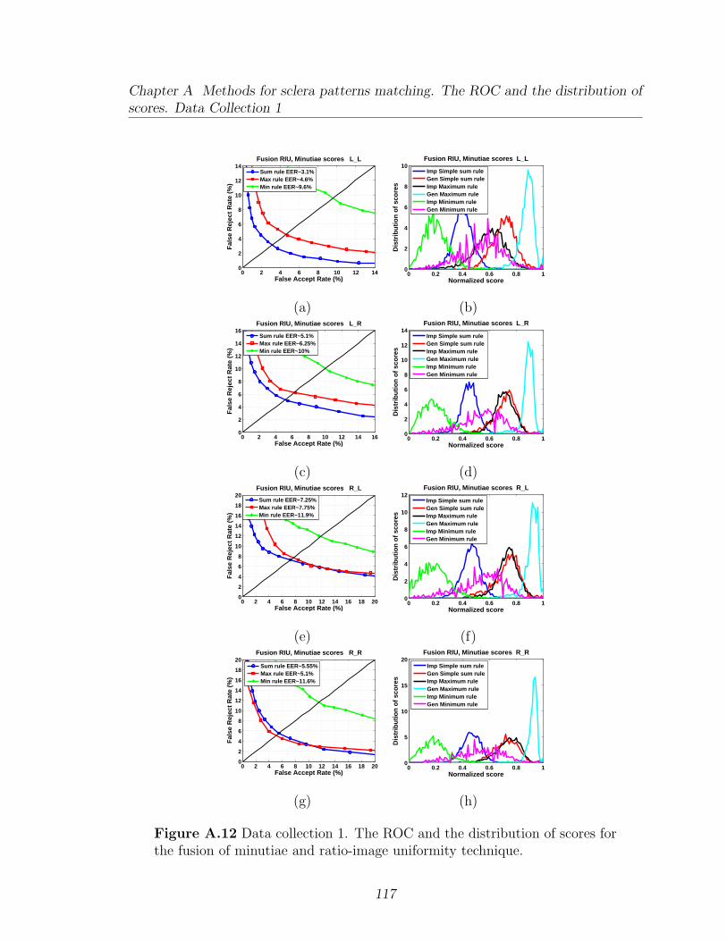
Chapter A Methods for sclera patterns matching. The ROC and the distribution ofscores. Data Collection 1
0 2 4 6 8 10 12 140
2
4
6
8
10
12
14Fusion RIU, Minutiae scores L_L
False Accept Rate (%)
Fal
se R
ejec
t R
ate
(%)
Sum rule EER~3.1%Max rule EER~4.6%Min rule EER~9.6%
0 0.2 0.4 0.6 0.8 10
2
4
6
8
10
Normalized score
Dis
trib
uti
on
of
sco
res
Fusion RIU, Minutiae scores L_L
Imp Simple sum ruleGen Simple sum ruleImp Maximum ruleGen Maximum ruleImp Minimum ruleGen Minimum rule
(a) (b)
0 2 4 6 8 10 12 14 160
2
4
6
8
10
12
14
16Fusion RIU, Minutiae scores L_R
False Accept Rate (%)
Fal
se R
ejec
t R
ate
(%)
Sum rule EER~5.1%Max rule EER~6.25%Min rule EER~10%
0 0.2 0.4 0.6 0.8 10
2
4
6
8
10
12
14
Normalized score
Dis
trib
uti
on
of
sco
res
Fusion RIU, Minutiae scores L_R
Imp Simple sum ruleGen Simple sum ruleImp Maximum ruleGen Maximum ruleImp Minimum ruleGen Minimum rule
(c) (d)
0 2 4 6 8 10 12 14 16 18 200
2
4
6
8
10
12
14
16
18
20Fusion RIU, Minutiae scores R_L
False Accept Rate (%)
Fal
se R
ejec
t R
ate
(%)
Sum rule EER~7.25%Max rule EER~7.75%Min rule EER~11.9%
0 0.2 0.4 0.6 0.8 10
2
4
6
8
10
12
Normalized score
Dis
trib
uti
on
of
sco
res
Fusion RIU, Minutiae scores R_L
Imp Simple sum ruleGen Simple sum ruleImp Maximum ruleGen Maximum ruleImp Minimum ruleGen Minimum rule
(e) (f)
0 2 4 6 8 10 12 14 16 18 200
2
4
6
8
10
12
14
16
18
20Fusion RIU, Minutiae scores R_R
False Accept Rate (%)
Fal
se R
ejec
t R
ate
(%)
Sum rule EER~5.55%Max rule EER~5.1%Min rule EER~11.6%
0 0.2 0.4 0.6 0.8 10
5
10
15
20
Normalized score
Dis
trib
uti
on
of
sco
res
Fusion RIU, Minutiae scores R_R
Imp Simple sum ruleGen Simple sum ruleImp Maximum ruleGen Maximum ruleImp Minimum ruleGen Minimum rule
(g) (h)
Figure A.12 Data collection 1. The ROC and the distribution of scores forthe fusion of minutiae and ratio-image uniformity technique.
117

Chapter A Methods for sclera patterns matching. The ROC and the distribution ofscores. Data Collection 1
0 1 2 3 4 5 6 7 8 9 10 110
1
2
3
4
5
6
7
8
9
10
11Fusion RMSE, Minutiae scores L_L
False Accept Rate (%)
Fal
se R
ejec
t R
ate
(%)
Sum rule EER~1.5%Max rule EER~1.5%Min rule EER~9.25%
0 0.2 0.4 0.6 0.8 10
2
4
6
8
10
Normalized score
Dis
trib
uti
on
of
sco
res
Fusion RMSE, Minutiae scores L_L
Imp Simple sum ruleGen Simple sum ruleImp Maximum ruleGen Maximum ruleImp Minimum ruleGen Minimum rule
(a) (b)
0 2 4 6 8 10 12 14 160
2
4
6
8
10
12
14
16Fusion RMSE, Minutiae scores L_R
False Accept Rate (%)
Fal
se R
ejec
t R
ate
(%)
Sum rule EER~3.75%Max rule EER~4.75%Min rule EER~10.1%
0 0.2 0.4 0.6 0.8 10
2
4
6
8
10
Normalized score
Dis
trib
uti
on
of
sco
res
Fusion RMSE, Minutiae scores L_R
Imp Simple sum ruleGen Simple sum ruleImp Maximum ruleGen Maximum ruleImp Minimum ruleGen Minimum rule
(c) (d)
0 2 4 6 8 10 12 14 16 18 200
2
4
6
8
10
12
14
16
18
20Fusion RMSE, Minutiae scores R_L
False Accept Rate (%)
Fal
se R
ejec
t R
ate
(%)
Sum rule EER~5%Max rule EER~5.5%Min rule EER~12%
0 0.2 0.4 0.6 0.8 10
1
2
3
4
5
6
7
8
Normalized score
Dis
trib
uti
on
of
sco
res
Fusion RMSE, Minutiae scores R_L
Imp Simple sum ruleGen Simple sum ruleImp Maximum ruleGen Maximum ruleImp Minimum ruleGen Minimum rule
(e) (f)
0 2 4 6 8 10 12 14 160
2
4
6
8
10
12
14
16Fusion RMSE, Minutiae scores R_R
False Accept Rate (%)
Fal
se R
ejec
t R
ate
(%)
Sum rule EER~2.95%Max rule EER~2%Min rule EER~11.6%
0 0.2 0.4 0.6 0.8 10
2
4
6
8
10
Normalized score
Dis
trib
uti
on
of
sco
res
Fusion RMSE, Minutiae scores R_R
Imp Simple sum ruleGen Simple sum ruleImp Maximum ruleGen Maximum ruleImp Minimum ruleGen Minimum rule
(g) (h)
Figure A.13 Data collection 1. The ROC and the distribution of scores forthe fusion of minutiae and root mean square error technique.
118
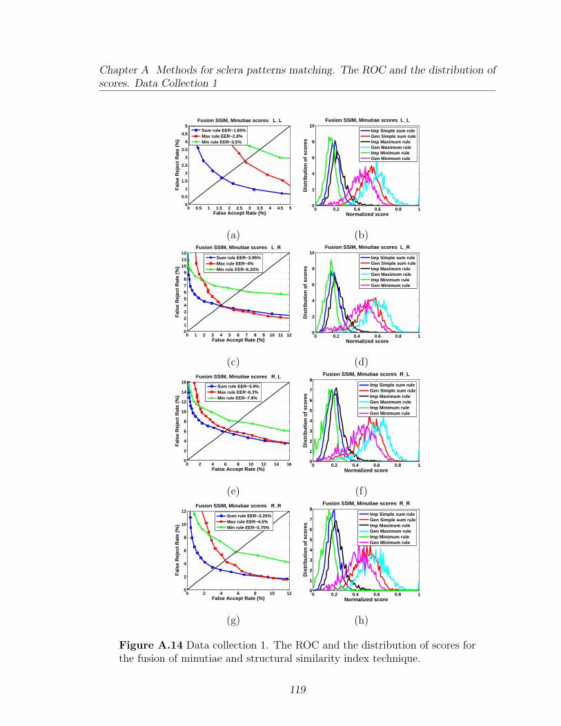
Chapter A Methods for sclera patterns matching. The ROC and the distribution ofscores. Data Collection 1
0 0.5 1 1.5 2 2.5 3 3.5 4 4.5 50
0.5
1
1.5
2
2.5
3
3.5
4
4.5
5Fusion SSIM, Minutiae scores L_L
False Accept Rate (%)
Fal
se R
ejec
t R
ate
(%)
Sum rule EER~1.65%Max rule EER~2.8%Min rule EER~3.5%
0 0.2 0.4 0.6 0.8 10
2
4
6
8
10
Normalized score
Dis
trib
uti
on
of
sco
res
Fusion SSIM, Minutiae scores L_L
Imp Simple sum ruleGen Simple sum ruleImp Maximum ruleGen Maximum ruleImp Minimum ruleGen Minimum rule
(a) (b)
0 1 2 3 4 5 6 7 8 9 10 11 120
123
456
789
101112
Fusion SSIM, Minutiae scores L_R
False Accept Rate (%)
Fal
se R
ejec
t R
ate
(%)
Sum rule EER~3.95%Max rule EER~4%Min rule EER~6.25%
0 0.2 0.4 0.6 0.8 10
2
4
6
8
10
Normalized score
Dis
trib
uti
on
of
sco
res
Fusion SSIM, Minutiae scores L_R
Imp Simple sum ruleGen Simple sum ruleImp Maximum ruleGen Maximum ruleImp Minimum ruleGen Minimum rule
(c) (d)
0 2 4 6 8 10 12 14 160
2
4
6
8
10
12
14
16Fusion SSIM, Minutiae scores R_L
False Accept Rate (%)
Fal
se R
ejec
t R
ate
(%)
Sum rule EER~5.9%Max rule EER~6.3%Min rule EER~7.9%
0 0.2 0.4 0.6 0.8 10
1
2
3
4
5
6
7
8
Normalized score
Dis
trib
uti
on
of
sco
res
Fusion SSIM, Minutiae scores R_L
Imp Simple sum ruleGen Simple sum ruleImp Maximum ruleGen Maximum ruleImp Minimum ruleGen Minimum rule
(e) (f)
0 2 4 6 8 10 120
2
4
6
8
10
12Fusion SSIM, Minutiae scores R_R
False Accept Rate (%)
Fal
se R
ejec
t R
ate
(%)
Sum rule EER~3.25%Max rule EER~4.5%Min rule EER~5.75%
0 0.2 0.4 0.6 0.8 10
1
2
3
4
5
6
7
8
Normalized score
Dis
trib
uti
on
of
sco
res
Fusion SSIM, Minutiae scores R_R
Imp Simple sum ruleGen Simple sum ruleImp Maximum ruleGen Maximum ruleImp Minimum ruleGen Minimum rule
(g) (h)
Figure A.14 Data collection 1. The ROC and the distribution of scores forthe fusion of minutiae and structural similarity index technique.
119
Appendix B
Fusion of iris patterns with scleral
patterns. The ROC and the
distribution of scores. Data
Collection 1
120
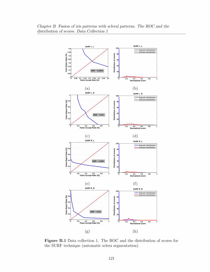
Chapter B Fusion of iris patterns with scleral patterns. The ROC and thedistribution of scores. Data Collection 1
0 0.05 0.1 0.15 0.2 0.25 0.3 0.35 0.40
0.05
0.1
0.15
0.2
0.25
0.3
0.35
0.4SURF L_L
False Accept Rate (%)
Fal
se R
ejec
t R
ate
(%)
EER ~ 0.225%
0 0.2 0.4 0.6 0.8 10
20
40
60
80
100
Normalized score
Dis
trib
uti
on
of
sco
res
SURF L_L
Imposter DistributionGenuine Distribution
(a) (b)
0 0.2 0.4 0.6 0.8 10
0.2
0.4
0.6
0.8
1SURF L_R
False Accept Rate (%)
Fal
se R
ejec
t R
ate
(%)
EER ~ 0.4%
0 0.2 0.4 0.6 0.8 10
20
40
60
80
100
Normalized score
Dis
trib
uti
on
of
sco
res
SURF L_R
Imposter DistributionGenuine Distribution
(c) (d)
0 0.2 0.4 0.6 0.8 10
0.2
0.4
0.6
0.8
1SURF R_L
False Accept Rate (%)
Fal
se R
ejec
t R
ate
(%)
EER ~ 0.28%
0 0.2 0.4 0.6 0.8 10
20
40
60
80
100
Normalized score
Dis
trib
uti
on
of
sco
res
SURF R_L
Imposter DistributionGenuine Distribution
(e) (f)
0 0.2 0.4 0.6 0.8 10
0.2
0.4
0.6
0.8
1SURF R_R
False Accept Rate (%)
Fal
se R
ejec
t R
ate
(%)
EER ~ 0.2%
0 0.2 0.4 0.6 0.8 10
20
40
60
80
100
Normalized score
Dis
trib
uti
on
of
sco
res
SURF R_R
Imposter DistributionGenuine Distribution
(g) (h)
Figure B.1 Data collection 1. The ROC and the distribution of scores forthe SURF technique (automatic sclera segmentation).
121
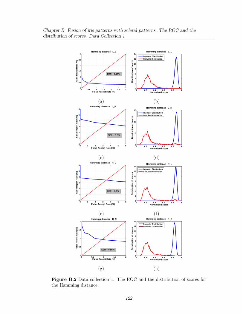
Chapter B Fusion of iris patterns with scleral patterns. The ROC and thedistribution of scores. Data Collection 1
0 0.5 1 1.5 2 2.5 30
0.5
1
1.5
2
2.5
3Hamming distance L_L
False Accept Rate (%)
Fal
se R
ejec
t R
ate
(%)
EER ~ 0.45%
0 0.2 0.4 0.6 0.8 10
2
4
6
8
10
12
14
Normalized score
Dis
trib
uti
on
of
sco
res
Hamming distance L_L
Imposter DistributionGenuine Distribution
(a) (b)
0 1 2 3 4 5 60
1
2
3
4
5
6Hamming distance L_R
False Accept Rate (%)
Fal
se R
ejec
t R
ate
(%)
EER ~ 3.5%
0 0.2 0.4 0.6 0.8 10
5
10
15
Normalized score
Dis
trib
uti
on
of
sco
res
Hamming distance L_R
Imposter DistributionGenuine Distribution
(c) (d)
0 1 2 3 4 5 60
1
2
3
4
5
6Hamming distance R_L
False Accept Rate (%)
Fal
se R
ejec
t R
ate
(%)
EER ~ 3.5%
0 0.2 0.4 0.6 0.8 10
2
4
6
8
10
12
14
Normalized score
Dis
trib
uti
on
of
sco
res
Hamming distance R_L
Imposter DistributionGenuine Distribution
(e) (f)
0 0.5 1 1.5 20
0.5
1
1.5
2Hamming distance R_R
False Accept Rate (%)
Fal
se R
ejec
t R
ate
(%)
EER ~ 0.95%
0 0.2 0.4 0.6 0.8 10
2
4
6
8
10
12
14
Normalized score
Dis
trib
uti
on
of
sco
res
Hamming distance R_R
Imposter DistributionGenuine Distribution
(g) (h)
Figure B.2 Data collection 1. The ROC and the distribution of scores forthe Hamming distance.
122
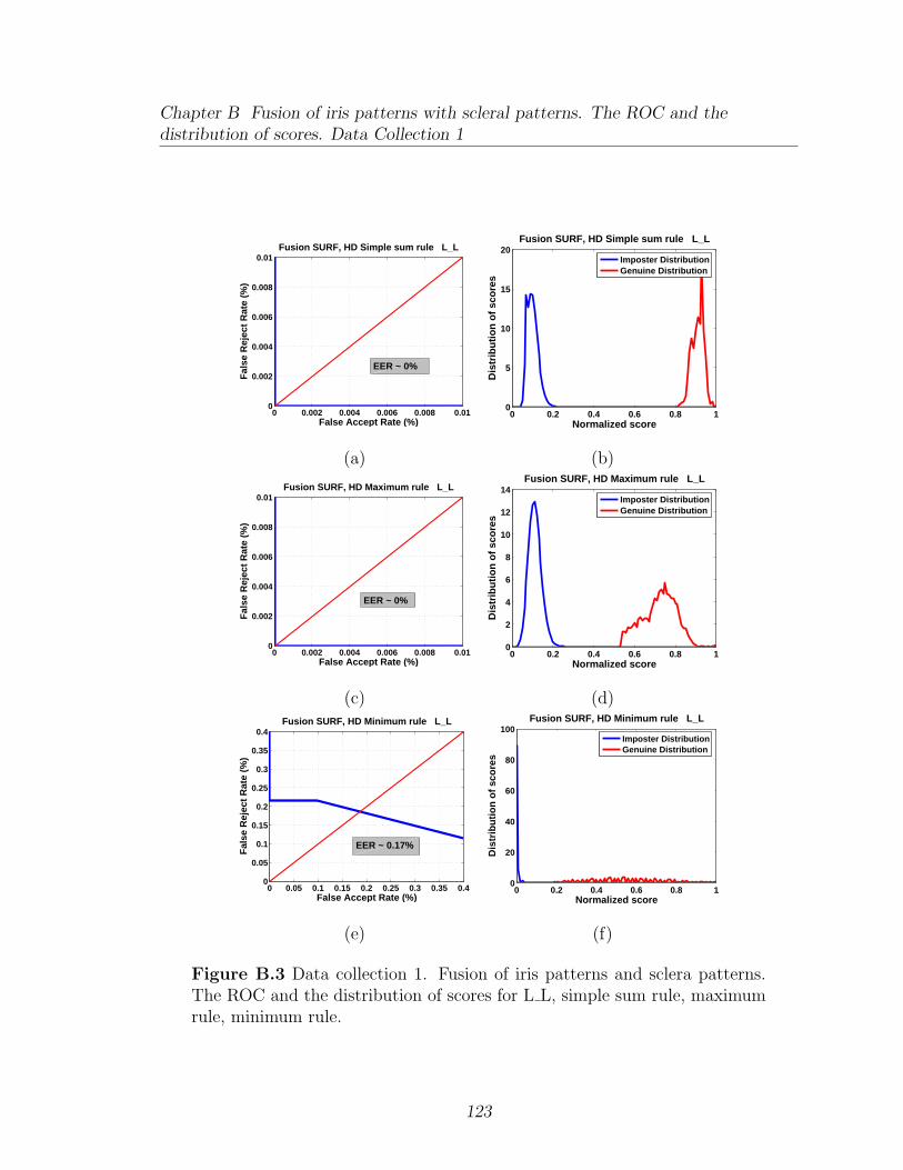
Chapter B Fusion of iris patterns with scleral patterns. The ROC and thedistribution of scores. Data Collection 1
0 0.002 0.004 0.006 0.008 0.010
0.002
0.004
0.006
0.008
0.01Fusion SURF, HD Simple sum rule L_L
False Accept Rate (%)
Fal
se R
ejec
t R
ate
(%)
EER ~ 0%
0 0.2 0.4 0.6 0.8 10
5
10
15
20
Normalized score
Dis
trib
uti
on
of
sco
res
Fusion SURF, HD Simple sum rule L_L
Imposter DistributionGenuine Distribution
(a) (b)
0 0.002 0.004 0.006 0.008 0.010
0.002
0.004
0.006
0.008
0.01Fusion SURF, HD Maximum rule L_L
False Accept Rate (%)
Fal
se R
ejec
t R
ate
(%)
EER ~ 0%
0 0.2 0.4 0.6 0.8 10
2
4
6
8
10
12
14
Normalized score
Dis
trib
uti
on
of
sco
res
Fusion SURF, HD Maximum rule L_L
Imposter DistributionGenuine Distribution
(c) (d)
0 0.05 0.1 0.15 0.2 0.25 0.3 0.35 0.40
0.05
0.1
0.15
0.2
0.25
0.3
0.35
0.4Fusion SURF, HD Minimum rule L_L
False Accept Rate (%)
Fal
se R
ejec
t R
ate
(%)
EER ~ 0.17%
0 0.2 0.4 0.6 0.8 10
20
40
60
80
100
Normalized score
Dis
trib
uti
on
of
sco
res
Fusion SURF, HD Minimum rule L_L
Imposter DistributionGenuine Distribution
(e) (f)
Figure B.3 Data collection 1. Fusion of iris patterns and sclera patterns.The ROC and the distribution of scores for L L, simple sum rule, maximumrule, minimum rule.
123
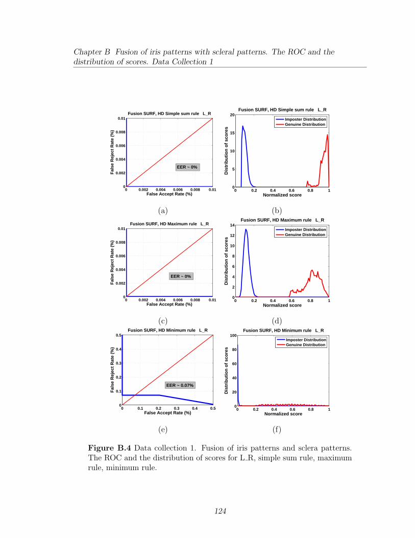
Chapter B Fusion of iris patterns with scleral patterns. The ROC and thedistribution of scores. Data Collection 1
0 0.002 0.004 0.006 0.008 0.010
0.002
0.004
0.006
0.008
0.01Fusion SURF, HD Simple sum rule L_R
False Accept Rate (%)
Fal
se R
ejec
t R
ate
(%)
EER ~ 0%
0 0.2 0.4 0.6 0.8 10
5
10
15
20
Normalized score
Dis
trib
uti
on
of
sco
res
Fusion SURF, HD Simple sum rule L_R
Imposter DistributionGenuine Distribution
(a) (b)
0 0.002 0.004 0.006 0.008 0.010
0.002
0.004
0.006
0.008
0.01Fusion SURF, HD Maximum rule L_R
False Accept Rate (%)
Fal
se R
ejec
t R
ate
(%)
EER ~ 0%
0 0.2 0.4 0.6 0.8 10
2
4
6
8
10
12
14
Normalized score
Dis
trib
uti
on
of
sco
res
Fusion SURF, HD Maximum rule L_R
Imposter DistributionGenuine Distribution
(c) (d)
0 0.1 0.2 0.3 0.4 0.50
0.1
0.2
0.3
0.4
0.5Fusion SURF, HD Minimum rule L_R
False Accept Rate (%)
Fal
se R
ejec
t R
ate
(%)
EER ~ 0.07%
0 0.2 0.4 0.6 0.8 10
20
40
60
80
100
Normalized score
Dis
trib
uti
on
of
sco
res
Fusion SURF, HD Minimum rule L_R
Imposter DistributionGenuine Distribution
(e) (f)
Figure B.4 Data collection 1. Fusion of iris patterns and sclera patterns.The ROC and the distribution of scores for L R, simple sum rule, maximumrule, minimum rule.
124
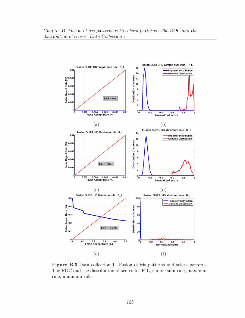
Chapter B Fusion of iris patterns with scleral patterns. The ROC and thedistribution of scores. Data Collection 1
0 0.002 0.004 0.006 0.008 0.010
0.002
0.004
0.006
0.008
0.01Fusion SURF, HD Simple sum rule R_L
False Accept Rate (%)
Fal
se R
ejec
t R
ate
(%)
EER ~ 0%
0 0.2 0.4 0.6 0.8 10
2
4
6
8
10
12
14
16
Normalized score
Dis
trib
uti
on
of
sco
res
Fusion SURF, HD Simple sum rule R_L
Imposter DistributionGenuine Distribution
(a) (b)
0 0.002 0.004 0.006 0.008 0.010
0.002
0.004
0.006
0.008
0.01Fusion SURF, HD Maximum rule R_L
False Accept Rate (%)
Fal
se R
ejec
t R
ate
(%)
EER ~ 0%
0 0.2 0.4 0.6 0.8 10
2
4
6
8
10
12
14
Normalized score
Dis
trib
uti
on
of
sco
res
Fusion SURF, HD Maximum rule R_L
Imposter DistributionGenuine Distribution
(c) (d)
0 0.1 0.2 0.3 0.4 0.50
0.1
0.2
0.3
0.4
0.5Fusion SURF, HD Minimum rule R_L
False Accept Rate (%)
Fal
se R
ejec
t R
ate
(%)
EER ~ 0.27%
0 0.2 0.4 0.6 0.8 10
20
40
60
80
100
Normalized score
Dis
trib
uti
on
of
sco
res
Fusion SURF, HD Minimum rule R_L
Imposter DistributionGenuine Distribution
(e) (f)
Figure B.5 Data collection 1. Fusion of iris patterns and sclera patterns.The ROC and the distribution of scores for R L, simple sum rule, maximumrule, minimum rule.
125
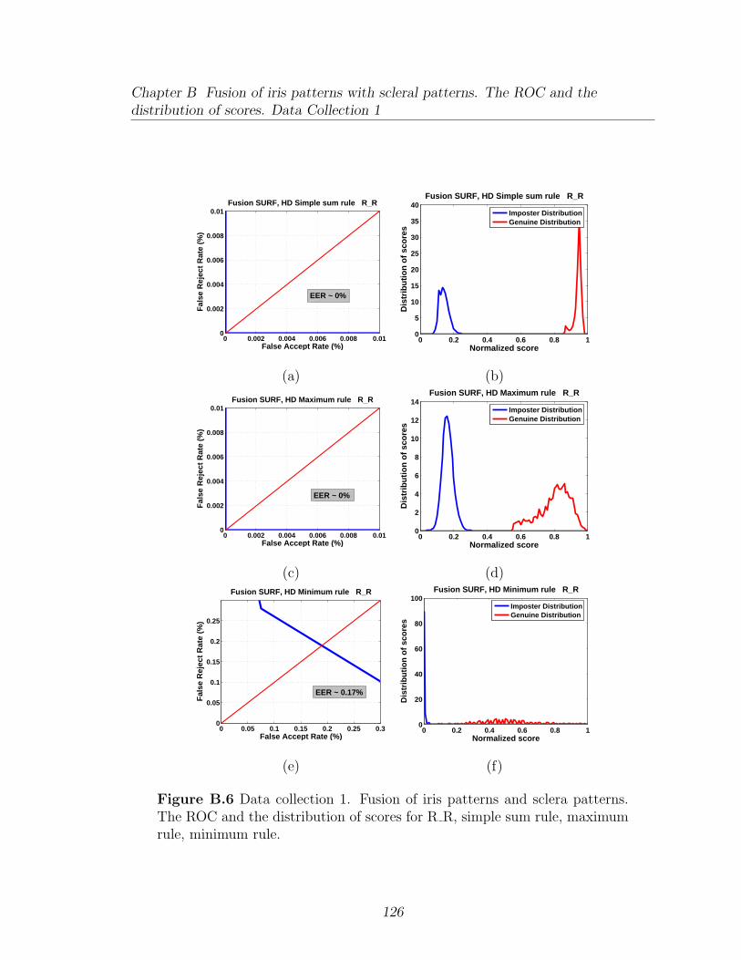
Chapter B Fusion of iris patterns with scleral patterns. The ROC and thedistribution of scores. Data Collection 1
0 0.002 0.004 0.006 0.008 0.010
0.002
0.004
0.006
0.008
0.01Fusion SURF, HD Simple sum rule R_R
False Accept Rate (%)
Fal
se R
ejec
t R
ate
(%)
EER ~ 0%
0 0.2 0.4 0.6 0.8 10
5
10
15
20
25
30
35
40
Normalized score
Dis
trib
uti
on
of
sco
res
Fusion SURF, HD Simple sum rule R_R
Imposter DistributionGenuine Distribution
(a) (b)
0 0.002 0.004 0.006 0.008 0.010
0.002
0.004
0.006
0.008
0.01Fusion SURF, HD Maximum rule R_R
False Accept Rate (%)
Fal
se R
ejec
t R
ate
(%)
EER ~ 0%
0 0.2 0.4 0.6 0.8 10
2
4
6
8
10
12
14
Normalized score
Dis
trib
uti
on
of
sco
res
Fusion SURF, HD Maximum rule R_R
Imposter DistributionGenuine Distribution
(c) (d)
0 0.05 0.1 0.15 0.2 0.25 0.30
0.05
0.1
0.15
0.2
0.25
Fusion SURF, HD Minimum rule R_R
False Accept Rate (%)
Fal
se R
ejec
t R
ate
(%)
EER ~ 0.17%
0 0.2 0.4 0.6 0.8 10
20
40
60
80
100
Normalized score
Dis
trib
uti
on
of
sco
res
Fusion SURF, HD Minimum rule R_R
Imposter DistributionGenuine Distribution
(e) (f)
Figure B.6 Data collection 1. Fusion of iris patterns and sclera patterns.The ROC and the distribution of scores for R R, simple sum rule, maximumrule, minimum rule.
126
Appendix C
Impact of intra-class variation.
The ROC and the distribution of
scores. Data collection 2.
127
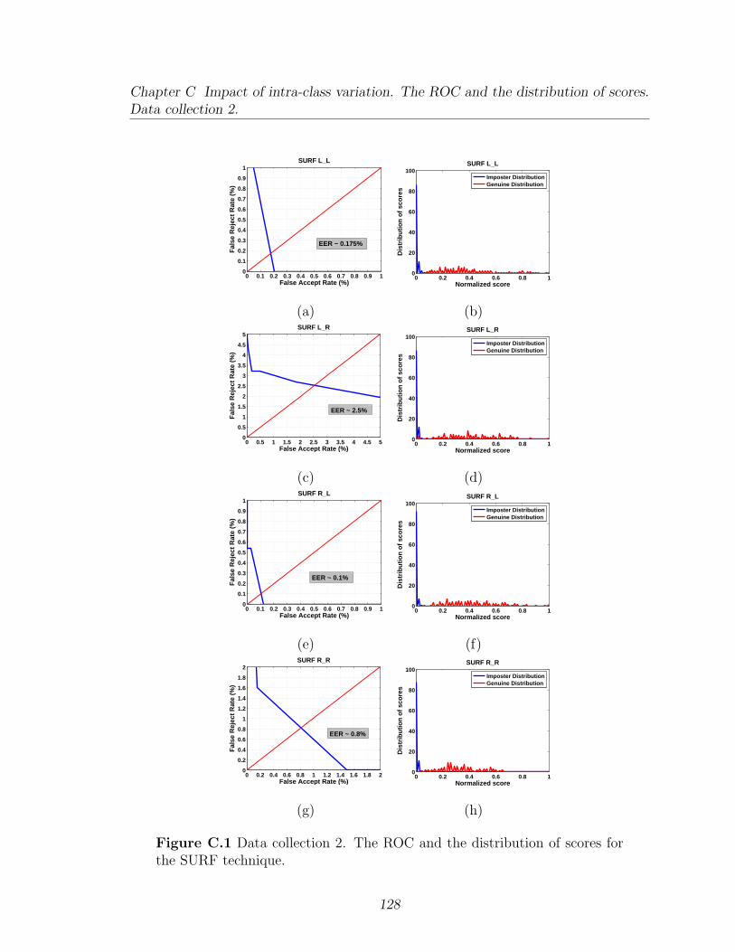
Chapter C Impact of intra-class variation. The ROC and the distribution of scores.Data collection 2.
0 0.1 0.2 0.3 0.4 0.5 0.6 0.7 0.8 0.9 10
0.1
0.2
0.3
0.4
0.5
0.6
0.7
0.8
0.9
1SURF L_L
False Accept Rate (%)
Fal
se R
ejec
t R
ate
(%)
EER ~ 0.175%
0 0.2 0.4 0.6 0.8 10
20
40
60
80
100
Normalized score
Dis
trib
uti
on
of
sco
res
SURF L_L
Imposter DistributionGenuine Distribution
(a) (b)
0 0.5 1 1.5 2 2.5 3 3.5 4 4.5 50
0.5
1
1.5
2
2.5
3
3.5
4
4.5
5SURF L_R
False Accept Rate (%)
Fal
se R
ejec
t R
ate
(%)
EER ~ 2.5%
0 0.2 0.4 0.6 0.8 10
20
40
60
80
100
Normalized score
Dis
trib
uti
on
of
sco
res
SURF L_R
Imposter DistributionGenuine Distribution
(c) (d)
0 0.1 0.2 0.3 0.4 0.5 0.6 0.7 0.8 0.9 10
0.1
0.2
0.3
0.4
0.5
0.6
0.7
0.8
0.9
1SURF R_L
False Accept Rate (%)
Fal
se R
ejec
t R
ate
(%)
EER ~ 0.1%
0 0.2 0.4 0.6 0.8 10
20
40
60
80
100
Normalized score
Dis
trib
uti
on
of
sco
res
SURF R_L
Imposter DistributionGenuine Distribution
(e) (f)
0 0.2 0.4 0.6 0.8 1 1.2 1.4 1.6 1.8 20
0.2
0.4
0.6
0.8
1
1.2
1.4
1.6
1.8
2SURF R_R
False Accept Rate (%)
Fal
se R
ejec
t R
ate
(%)
EER ~ 0.8%
0 0.2 0.4 0.6 0.8 10
20
40
60
80
100
Normalized score
Dis
trib
uti
on
of
sco
res
SURF R_R
Imposter DistributionGenuine Distribution
(g) (h)
Figure C.1 Data collection 2. The ROC and the distribution of scores forthe SURF technique.
128
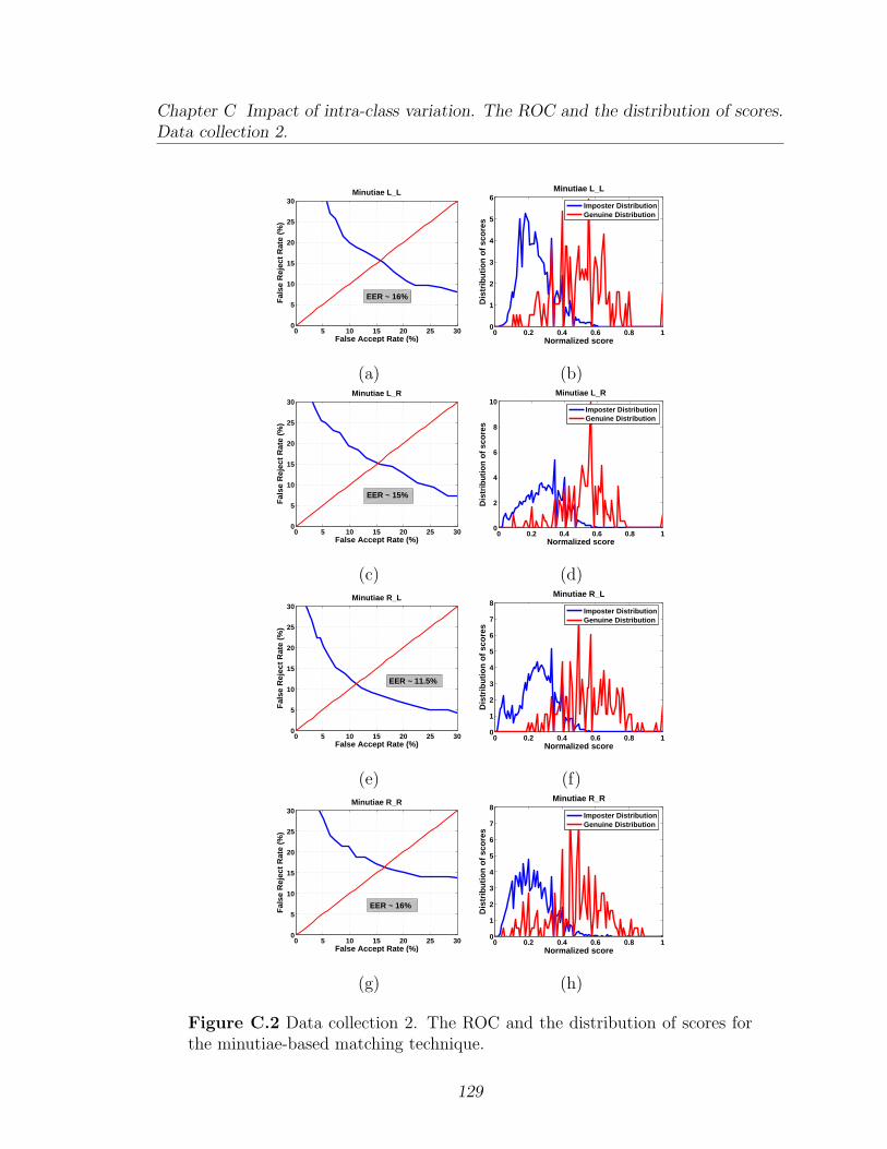
Chapter C Impact of intra-class variation. The ROC and the distribution of scores.Data collection 2.
0 5 10 15 20 25 300
5
10
15
20
25
30Minutiae L_L
False Accept Rate (%)
Fal
se R
ejec
t R
ate
(%)
EER ~ 16%
0 0.2 0.4 0.6 0.8 10
1
2
3
4
5
6
Normalized score
Dis
trib
uti
on
of
sco
res
Minutiae L_L
Imposter DistributionGenuine Distribution
(a) (b)
0 5 10 15 20 25 300
5
10
15
20
25
30Minutiae L_R
False Accept Rate (%)
Fal
se R
ejec
t R
ate
(%)
EER ~ 15%
0 0.2 0.4 0.6 0.8 10
2
4
6
8
10
Normalized score
Dis
trib
uti
on
of
sco
res
Minutiae L_R
Imposter DistributionGenuine Distribution
(c) (d)
0 5 10 15 20 25 300
5
10
15
20
25
30Minutiae R_L
False Accept Rate (%)
Fal
se R
ejec
t R
ate
(%)
EER ~ 11.5%
0 0.2 0.4 0.6 0.8 10
1
2
3
4
5
6
7
8
Normalized score
Dis
trib
uti
on
of
sco
res
Minutiae R_L
Imposter DistributionGenuine Distribution
(e) (f)
0 5 10 15 20 25 300
5
10
15
20
25
30Minutiae R_R
False Accept Rate (%)
Fal
se R
ejec
t R
ate
(%)
EER ~ 16%
0 0.2 0.4 0.6 0.8 10
1
2
3
4
5
6
7
8
Normalized score
Dis
trib
uti
on
of
sco
res
Minutiae R_R
Imposter DistributionGenuine Distribution
(g) (h)
Figure C.2 Data collection 2. The ROC and the distribution of scores forthe minutiae-based matching technique.
129
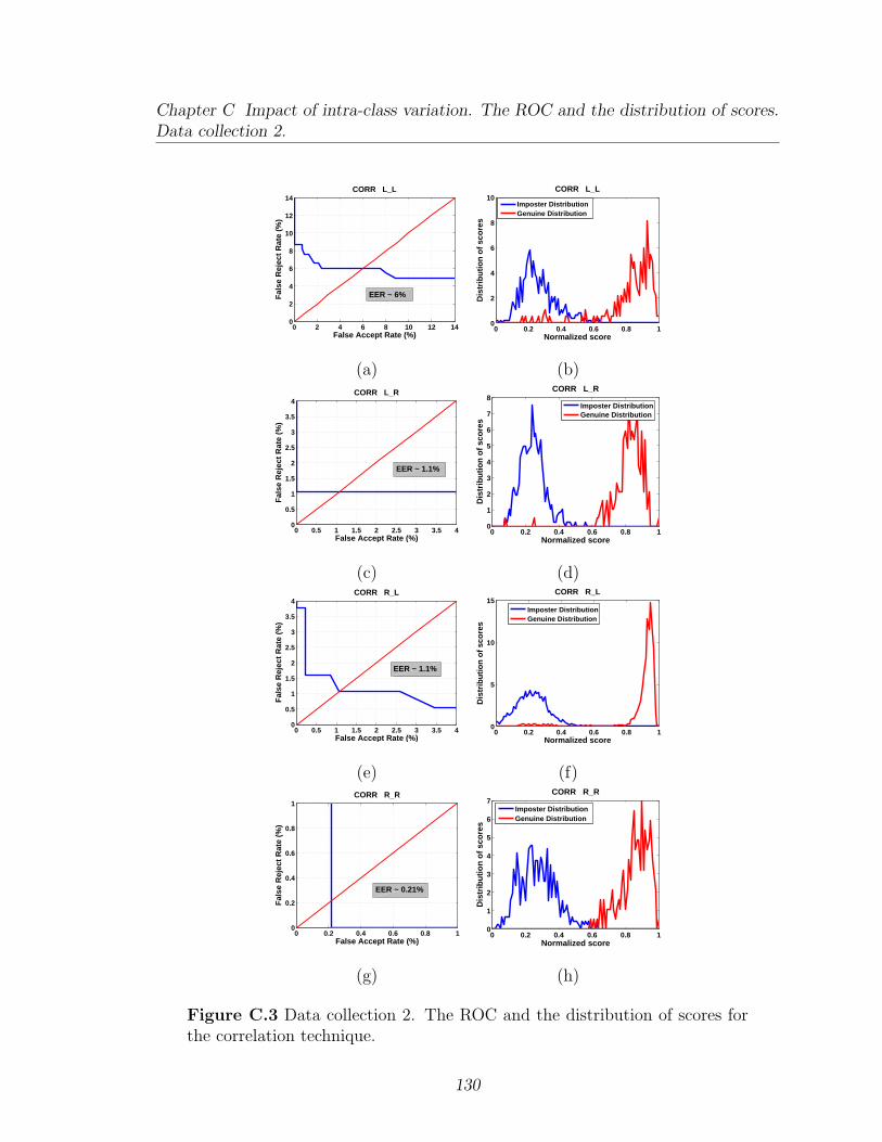
Chapter C Impact of intra-class variation. The ROC and the distribution of scores.Data collection 2.
0 2 4 6 8 10 12 140
2
4
6
8
10
12
14CORR L_L
False Accept Rate (%)
Fal
se R
ejec
t R
ate
(%)
EER ~ 6%
0 0.2 0.4 0.6 0.8 10
2
4
6
8
10
Normalized score
Dis
trib
uti
on
of
sco
res
CORR L_L
Imposter DistributionGenuine Distribution
(a) (b)
0 0.5 1 1.5 2 2.5 3 3.5 40
0.5
1
1.5
2
2.5
3
3.5
4CORR L_R
False Accept Rate (%)
Fal
se R
ejec
t R
ate
(%)
EER ~ 1.1%
0 0.2 0.4 0.6 0.8 10
1
2
3
4
5
6
7
8
Normalized score
Dis
trib
uti
on
of
sco
res
CORR L_R
Imposter DistributionGenuine Distribution
(c) (d)
0 0.5 1 1.5 2 2.5 3 3.5 40
0.5
1
1.5
2
2.5
3
3.5
4CORR R_L
False Accept Rate (%)
Fal
se R
ejec
t R
ate
(%)
EER ~ 1.1%
0 0.2 0.4 0.6 0.8 10
5
10
15
Normalized score
Dis
trib
uti
on
of
sco
res
CORR R_L
Imposter DistributionGenuine Distribution
(e) (f)
0 0.2 0.4 0.6 0.8 10
0.2
0.4
0.6
0.8
1CORR R_R
False Accept Rate (%)
Fal
se R
ejec
t R
ate
(%)
EER ~ 0.21%
0 0.2 0.4 0.6 0.8 10
1
2
3
4
5
6
7
Normalized score
Dis
trib
uti
on
of
sco
res
CORR R_R
Imposter DistributionGenuine Distribution
(g) (h)
Figure C.3 Data collection 2. The ROC and the distribution of scores forthe correlation technique.
130
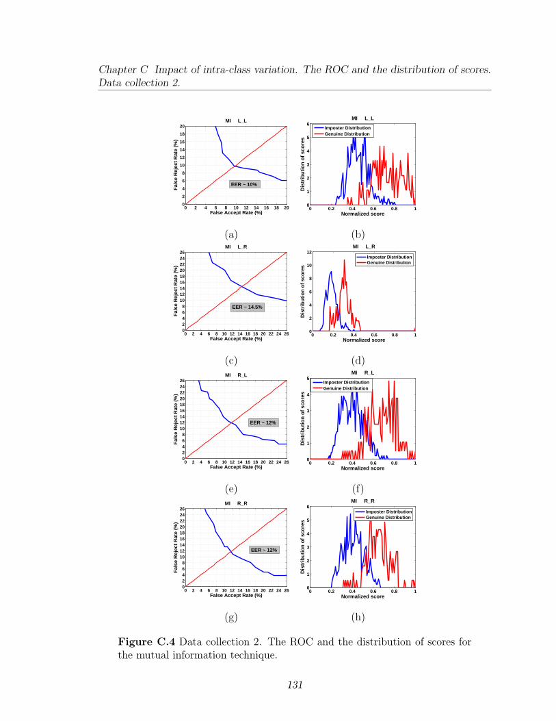
Chapter C Impact of intra-class variation. The ROC and the distribution of scores.Data collection 2.
0 2 4 6 8 10 12 14 16 18 200
2
4
6
8
10
12
14
16
18
20MI L_L
False Accept Rate (%)
Fal
se R
ejec
t R
ate
(%)
EER ~ 10%
0 0.2 0.4 0.6 0.8 10
1
2
3
4
5
6
Normalized score
Dis
trib
uti
on
of
sco
res
MI L_L
Imposter DistributionGenuine Distribution
(a) (b)
0 2 4 6 8 10 12 14 16 18 20 22 24 2602468
101214161820222426
MI L_R
False Accept Rate (%)
Fal
se R
ejec
t R
ate
(%)
EER ~ 14.5%
0 0.2 0.4 0.6 0.8 10
2
4
6
8
10
12
Normalized score
Dis
trib
uti
on
of
sco
res
MI L_R
Imposter DistributionGenuine Distribution
(c) (d)
0 2 4 6 8 10 12 14 16 18 20 22 24 2602468
101214161820222426
MI R_L
False Accept Rate (%)
Fal
se R
ejec
t R
ate
(%)
EER ~ 12%
0 0.2 0.4 0.6 0.8 10
1
2
3
4
5
Normalized score
Dis
trib
uti
on
of
sco
res
MI R_L
Imposter DistributionGenuine Distribution
(e) (f)
0 2 4 6 8 10 12 14 16 18 20 22 24 2602468
101214161820222426
MI R_R
False Accept Rate (%)
Fal
se R
ejec
t R
ate
(%)
EER ~ 12%
0 0.2 0.4 0.6 0.8 10
1
2
3
4
5
6
Normalized score
Dis
trib
uti
on
of
sco
res
MI R_R
Imposter DistributionGenuine Distribution
(g) (h)
Figure C.4 Data collection 2. The ROC and the distribution of scores forthe mutual information technique.
131
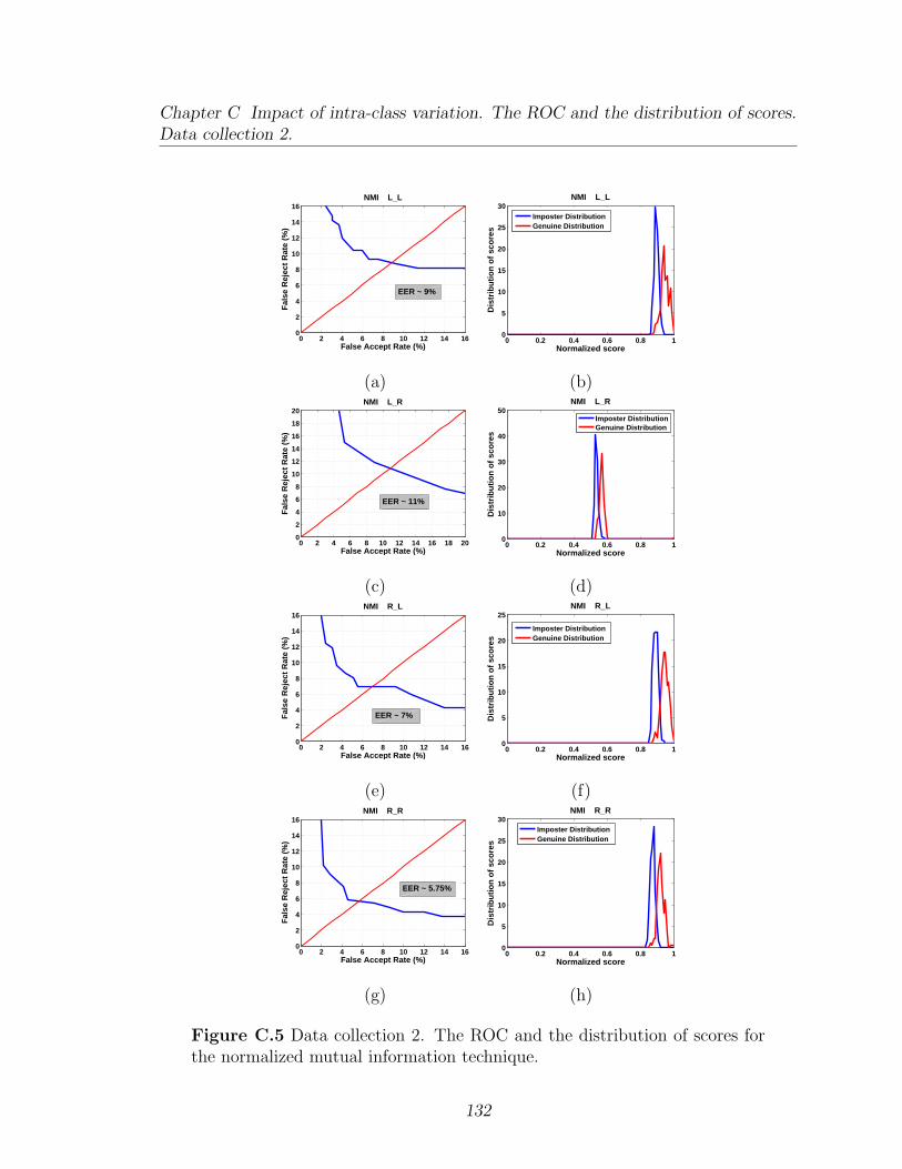
Chapter C Impact of intra-class variation. The ROC and the distribution of scores.Data collection 2.
0 2 4 6 8 10 12 14 160
2
4
6
8
10
12
14
16NMI L_L
False Accept Rate (%)
Fal
se R
ejec
t R
ate
(%)
EER ~ 9%
0 0.2 0.4 0.6 0.8 10
5
10
15
20
25
30
Normalized score
Dis
trib
uti
on
of
sco
res
NMI L_L
Imposter DistributionGenuine Distribution
(a) (b)
0 2 4 6 8 10 12 14 16 18 200
2
4
6
8
10
12
14
16
18
20NMI L_R
False Accept Rate (%)
Fal
se R
ejec
t R
ate
(%)
EER ~ 11%
0 0.2 0.4 0.6 0.8 10
10
20
30
40
50
Normalized score
Dis
trib
uti
on
of
sco
res
NMI L_R
Imposter DistributionGenuine Distribution
(c) (d)
0 2 4 6 8 10 12 14 160
2
4
6
8
10
12
14
16NMI R_L
False Accept Rate (%)
Fal
se R
ejec
t R
ate
(%)
EER ~ 7%
0 0.2 0.4 0.6 0.8 10
5
10
15
20
25
Normalized score
Dis
trib
uti
on
of
sco
res
NMI R_L
Imposter DistributionGenuine Distribution
(e) (f)
0 2 4 6 8 10 12 14 160
2
4
6
8
10
12
14
16NMI R_R
False Accept Rate (%)
Fal
se R
ejec
t R
ate
(%)
EER ~ 5.75%
0 0.2 0.4 0.6 0.8 10
5
10
15
20
25
30
Normalized score
Dis
trib
uti
on
of
sco
res
NMI R_R
Imposter DistributionGenuine Distribution
(g) (h)
Figure C.5 Data collection 2. The ROC and the distribution of scores forthe normalized mutual information technique.
132
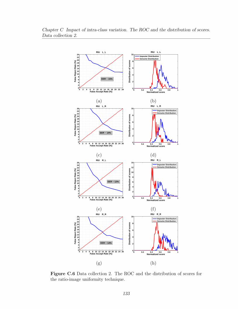
Chapter C Impact of intra-class variation. The ROC and the distribution of scores.Data collection 2.
0 2 4 6 8 10 12 14 16 18 20 22 240
246
81012
141618
202224
RIU L_L
False Accept Rate (%)
Fal
se R
ejec
t R
ate
(%)
EER ~ 15%
0 0.2 0.4 0.6 0.8 10
2
4
6
8
10
Normalized score
Dis
trib
uti
on
of
sco
res
RIU L_L
Imposter DistributionGenuine Distribution
(a) (b)
0 2 4 6 8 10 12 14 16 18 20 22 24 2602468
101214161820222426
RIU L_R
False Accept Rate (%)
Fal
se R
ejec
t R
ate
(%)
EER ~ 14%
0 0.2 0.4 0.6 0.8 10
2
4
6
8
10
Normalized score
Dis
trib
uti
on
of
sco
res
RIU L_R
Imposter DistributionGenuine Distribution
(c) (d)
0 2 4 6 8 10 12 14 16 18 20 22 24 2602468
101214161820222426
RIU R_L
False Accept Rate (%)
Fal
se R
ejec
t R
ate
(%)
EER ~ 12%
0 0.2 0.4 0.6 0.8 10
2
4
6
8
10
12
14
Normalized score
Dis
trib
uti
on
of
sco
res
RIU R_L
Imposter DistributionGenuine Distribution
(e) (f)
0 2 4 6 8 10 12 14 16 18 20 22 24 2602468
101214161820222426
RIU R_R
False Accept Rate (%)
Fal
se R
ejec
t R
ate
(%)
EER ~ 14%
0 0.2 0.4 0.6 0.8 10
2
4
6
8
10
Normalized score
Dis
trib
uti
on
of
sco
res
RIU R_R
Imposter DistributionGenuine Distribution
(g) (h)
Figure C.6 Data collection 2. The ROC and the distribution of scores forthe ratio-image uniformity technique.
133
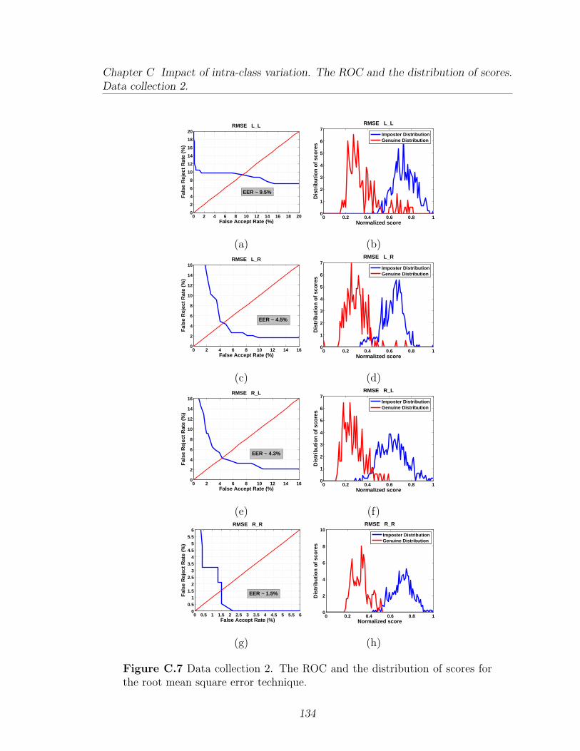
Chapter C Impact of intra-class variation. The ROC and the distribution of scores.Data collection 2.
0 2 4 6 8 10 12 14 16 18 200
2
4
6
8
10
12
14
16
18
20RMSE L_L
False Accept Rate (%)
Fal
se R
ejec
t R
ate
(%)
EER ~ 9.5%
0 0.2 0.4 0.6 0.8 10
1
2
3
4
5
6
7
Normalized score
Dis
trib
uti
on
of
sco
res
RMSE L_L
Imposter DistributionGenuine Distribution
(a) (b)
0 2 4 6 8 10 12 14 160
2
4
6
8
10
12
14
16RMSE L_R
False Accept Rate (%)
Fal
se R
ejec
t R
ate
(%)
EER ~ 4.5%
0 0.2 0.4 0.6 0.8 10
1
2
3
4
5
6
7
Normalized score
Dis
trib
uti
on
of
sco
res
RMSE L_R
Imposter DistributionGenuine Distribution
(c) (d)
0 2 4 6 8 10 12 14 160
2
4
6
8
10
12
14
16RMSE R_L
False Accept Rate (%)
Fal
se R
ejec
t R
ate
(%)
EER ~ 4.3%
0 0.2 0.4 0.6 0.8 10
1
2
3
4
5
6
7
Normalized score
Dis
trib
uti
on
of
sco
res
RMSE R_L
Imposter DistributionGenuine Distribution
(e) (f)
0 0.5 1 1.5 2 2.5 3 3.5 4 4.5 5 5.5 60
0.51
1.5
22.5
3
3.54
4.5
55.5
6RMSE R_R
False Accept Rate (%)
Fal
se R
ejec
t R
ate
(%)
EER ~ 1.5%
0 0.2 0.4 0.6 0.8 10
2
4
6
8
10
Normalized score
Dis
trib
uti
on
of
sco
res
RMSE R_R
Imposter DistributionGenuine Distribution
(g) (h)
Figure C.7 Data collection 2. The ROC and the distribution of scores forthe root mean square error technique.
134
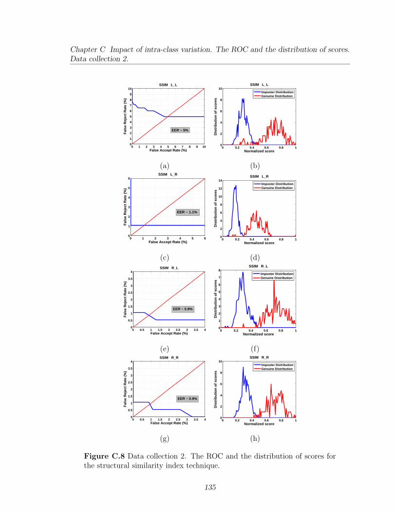
Chapter C Impact of intra-class variation. The ROC and the distribution of scores.Data collection 2.
0 1 2 3 4 5 6 7 8 9 100
1
2
3
4
5
6
7
8
9
10SSIM L_L
False Accept Rate (%)
Fal
se R
ejec
t R
ate
(%)
EER ~ 5%
0 0.2 0.4 0.6 0.8 10
2
4
6
8
10
Normalized score
Dis
trib
uti
on
of
sco
res
SSIM L_L
Imposter DistributionGenuine Distribution
(a) (b)
0 1 2 3 4 5 60
1
2
3
4
5
6SSIM L_R
False Accept Rate (%)
Fal
se R
ejec
t R
ate
(%)
EER ~ 1.1%
0 0.2 0.4 0.6 0.8 10
2
4
6
8
10
12
14
Normalized score
Dis
trib
uti
on
of
sco
res
SSIM L_R
Imposter DistributionGenuine Distribution
(c) (d)
0 0.5 1 1.5 2 2.5 3 3.5 40
0.5
1
1.5
2
2.5
3
3.5
4SSIM R_L
False Accept Rate (%)
Fal
se R
ejec
t R
ate
(%)
EER ~ 0.9%
0 0.2 0.4 0.6 0.8 10
1
2
3
4
5
6
7
8
Normalized score
Dis
trib
uti
on
of
sco
res
SSIM R_L
Imposter DistributionGenuine Distribution
(e) (f)
0 0.5 1 1.5 2 2.5 3 3.5 40
0.5
1
1.5
2
2.5
3
3.5
4SSIM R_R
False Accept Rate (%)
Fal
se R
ejec
t R
ate
(%)
EER ~ 0.9%
0 0.2 0.4 0.6 0.8 10
2
4
6
8
10
Normalized score
Dis
trib
uti
on
of
sco
res
SSIM R_R
Imposter DistributionGenuine Distribution
(g) (h)
Figure C.8 Data collection 2. The ROC and the distribution of scores forthe structural similarity index technique.
135
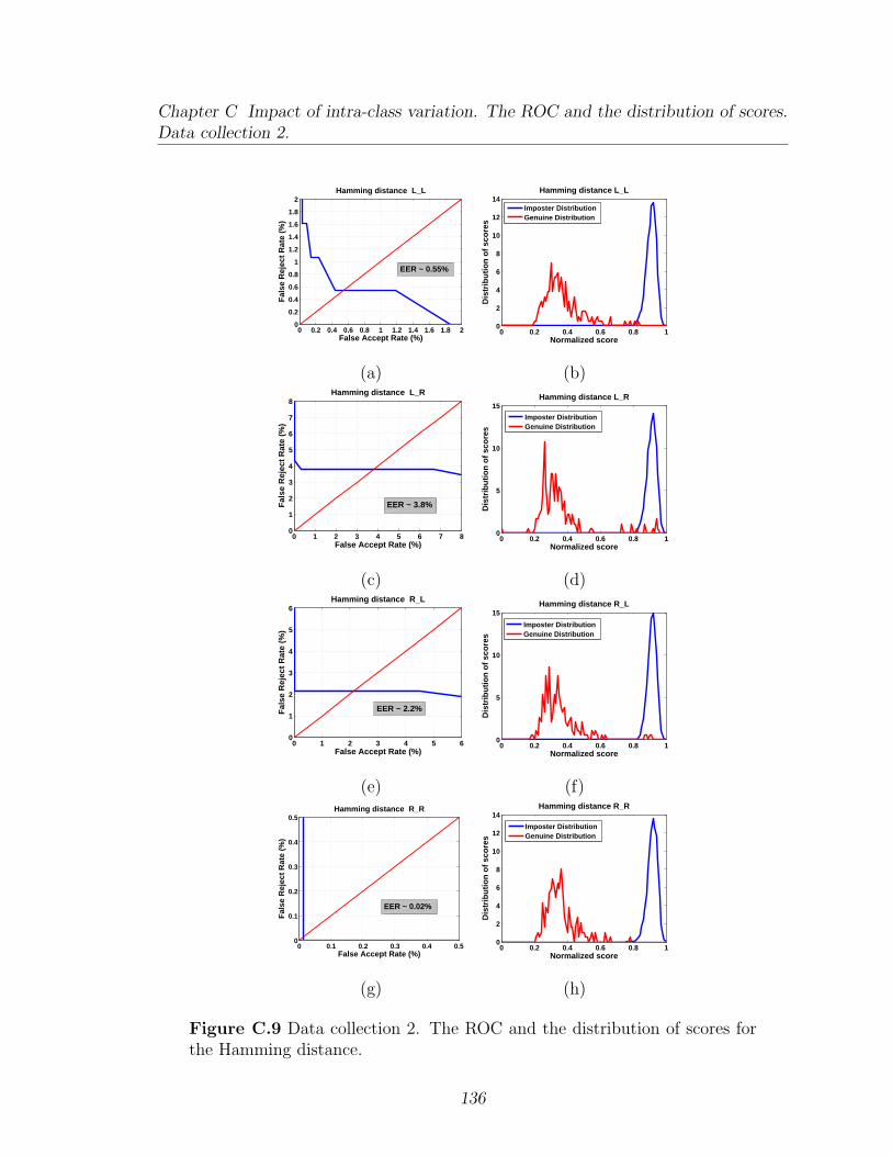
Chapter C Impact of intra-class variation. The ROC and the distribution of scores.Data collection 2.
0 0.2 0.4 0.6 0.8 1 1.2 1.4 1.6 1.8 20
0.2
0.4
0.6
0.8
1
1.2
1.4
1.6
1.8
2Hamming distance L_L
False Accept Rate (%)
Fal
se R
ejec
t R
ate
(%)
EER ~ 0.55%
0 0.2 0.4 0.6 0.8 10
2
4
6
8
10
12
14
Normalized score
Dis
trib
uti
on
of
sco
res
Hamming distance L_L
Imposter DistributionGenuine Distribution
(a) (b)
0 1 2 3 4 5 6 7 80
1
2
3
4
5
6
7
8Hamming distance L_R
False Accept Rate (%)
Fal
se R
ejec
t R
ate
(%)
EER ~ 3.8%
0 0.2 0.4 0.6 0.8 10
5
10
15
Normalized score
Dis
trib
uti
on
of
sco
res
Hamming distance L_R
Imposter DistributionGenuine Distribution
(c) (d)
0 1 2 3 4 5 60
1
2
3
4
5
6Hamming distance R_L
False Accept Rate (%)
Fal
se R
ejec
t R
ate
(%)
EER ~ 2.2%
0 0.2 0.4 0.6 0.8 10
5
10
15
Normalized score
Dis
trib
uti
on
of
sco
res
Hamming distance R_L
Imposter DistributionGenuine Distribution
(e) (f)
0 0.1 0.2 0.3 0.4 0.50
0.1
0.2
0.3
0.4
0.5Hamming distance R_R
False Accept Rate (%)
Fal
se R
ejec
t R
ate
(%)
EER ~ 0.02%
0 0.2 0.4 0.6 0.8 10
2
4
6
8
10
12
14
Normalized score
Dis
trib
uti
on
of
sco
res
Hamming distance R_R
Imposter DistributionGenuine Distribution
(g) (h)
Figure C.9 Data collection 2. The ROC and the distribution of scores forthe Hamming distance.
136
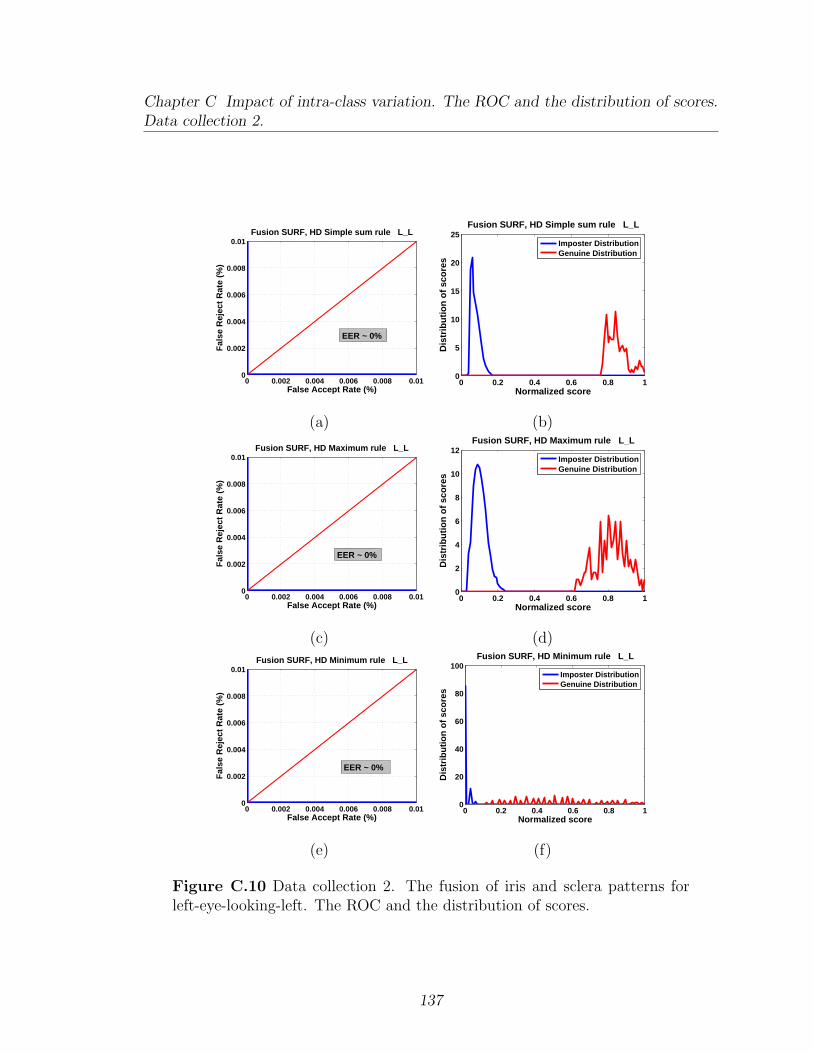
Chapter C Impact of intra-class variation. The ROC and the distribution of scores.Data collection 2.
0 0.002 0.004 0.006 0.008 0.010
0.002
0.004
0.006
0.008
0.01Fusion SURF, HD Simple sum rule L_L
False Accept Rate (%)
Fal
se R
ejec
t R
ate
(%)
EER ~ 0%
0 0.2 0.4 0.6 0.8 10
5
10
15
20
25
Normalized score
Dis
trib
uti
on
of
sco
res
Fusion SURF, HD Simple sum rule L_L
Imposter DistributionGenuine Distribution
(a) (b)
0 0.002 0.004 0.006 0.008 0.010
0.002
0.004
0.006
0.008
0.01Fusion SURF, HD Maximum rule L_L
False Accept Rate (%)
Fal
se R
ejec
t R
ate
(%)
EER ~ 0%
0 0.2 0.4 0.6 0.8 10
2
4
6
8
10
12
Normalized score
Dis
trib
uti
on
of
sco
res
Fusion SURF, HD Maximum rule L_L
Imposter DistributionGenuine Distribution
(c) (d)
0 0.002 0.004 0.006 0.008 0.010
0.002
0.004
0.006
0.008
0.01Fusion SURF, HD Minimum rule L_L
False Accept Rate (%)
Fal
se R
ejec
t R
ate
(%)
EER ~ 0%
0 0.2 0.4 0.6 0.8 10
20
40
60
80
100
Normalized score
Dis
trib
uti
on
of
sco
res
Fusion SURF, HD Minimum rule L_L
Imposter DistributionGenuine Distribution
(e) (f)
Figure C.10 Data collection 2. The fusion of iris and sclera patterns forleft-eye-looking-left. The ROC and the distribution of scores.
137
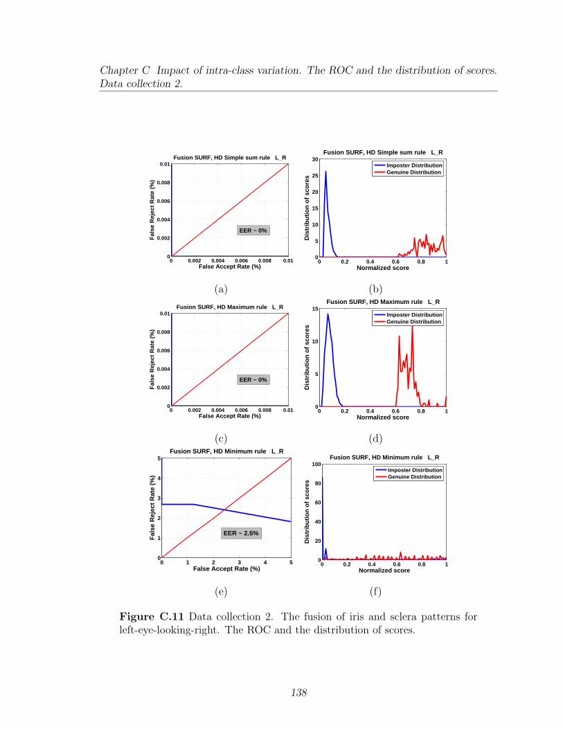
Chapter C Impact of intra-class variation. The ROC and the distribution of scores.Data collection 2.
0 0.002 0.004 0.006 0.008 0.010
0.002
0.004
0.006
0.008
0.01Fusion SURF, HD Simple sum rule L_R
False Accept Rate (%)
Fal
se R
ejec
t R
ate
(%)
EER ~ 0%
0 0.2 0.4 0.6 0.8 10
5
10
15
20
25
30
Normalized score
Dis
trib
uti
on
of
sco
res
Fusion SURF, HD Simple sum rule L_R
Imposter DistributionGenuine Distribution
(a) (b)
0 0.002 0.004 0.006 0.008 0.010
0.002
0.004
0.006
0.008
0.01Fusion SURF, HD Maximum rule L_R
False Accept Rate (%)
Fal
se R
ejec
t R
ate
(%)
EER ~ 0%
0 0.2 0.4 0.6 0.8 10
5
10
15
Normalized score
Dis
trib
uti
on
of
sco
res
Fusion SURF, HD Maximum rule L_R
Imposter DistributionGenuine Distribution
(c) (d)
0 1 2 3 4 50
1
2
3
4
5Fusion SURF, HD Minimum rule L_R
False Accept Rate (%)
Fal
se R
ejec
t R
ate
(%)
EER ~ 2.5%
0 0.2 0.4 0.6 0.8 10
20
40
60
80
100
Normalized score
Dis
trib
uti
on
of
sco
res
Fusion SURF, HD Minimum rule L_R
Imposter DistributionGenuine Distribution
(e) (f)
Figure C.11 Data collection 2. The fusion of iris and sclera patterns forleft-eye-looking-right. The ROC and the distribution of scores.
138
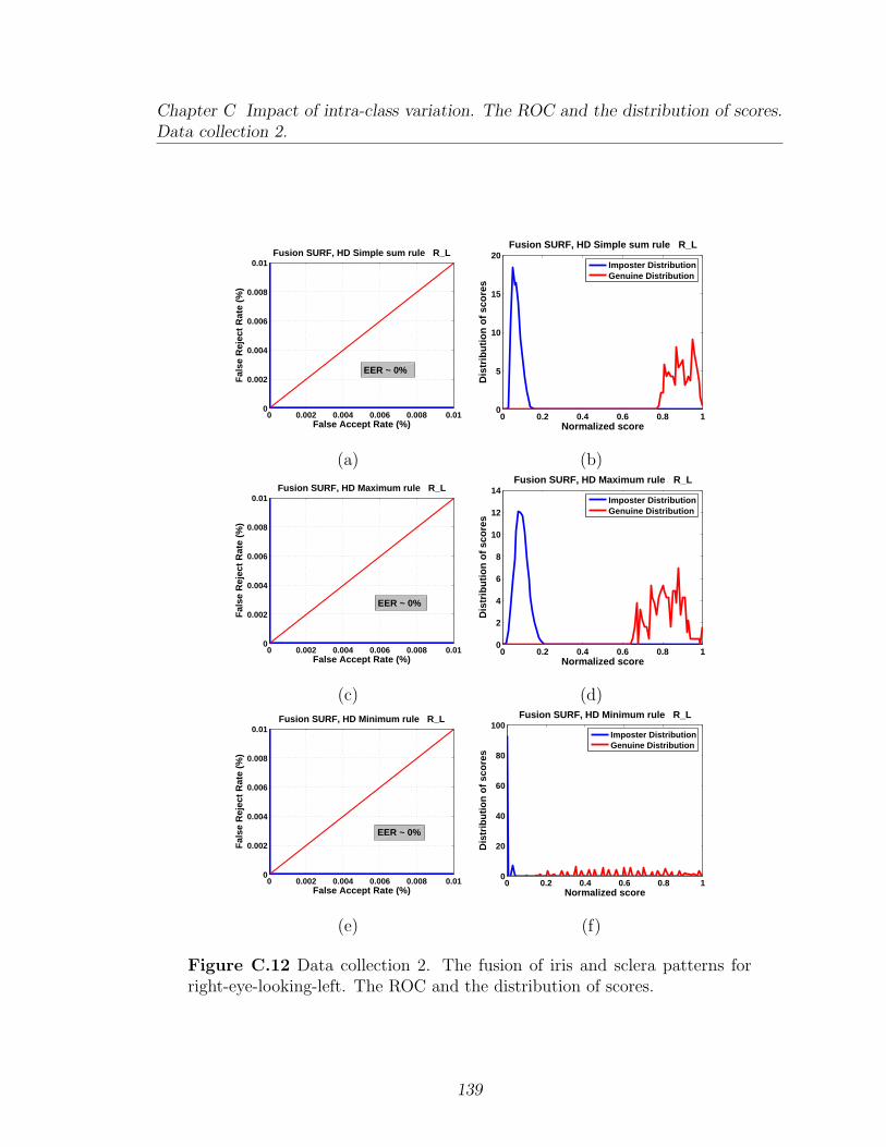
Chapter C Impact of intra-class variation. The ROC and the distribution of scores.Data collection 2.
0 0.002 0.004 0.006 0.008 0.010
0.002
0.004
0.006
0.008
0.01Fusion SURF, HD Simple sum rule R_L
False Accept Rate (%)
Fal
se R
ejec
t R
ate
(%)
EER ~ 0%
0 0.2 0.4 0.6 0.8 10
5
10
15
20
Normalized score
Dis
trib
uti
on
of
sco
res
Fusion SURF, HD Simple sum rule R_L
Imposter DistributionGenuine Distribution
(a) (b)
0 0.002 0.004 0.006 0.008 0.010
0.002
0.004
0.006
0.008
0.01Fusion SURF, HD Maximum rule R_L
False Accept Rate (%)
Fal
se R
ejec
t R
ate
(%)
EER ~ 0%
0 0.2 0.4 0.6 0.8 10
2
4
6
8
10
12
14
Normalized score
Dis
trib
uti
on
of
sco
res
Fusion SURF, HD Maximum rule R_L
Imposter DistributionGenuine Distribution
(c) (d)
0 0.002 0.004 0.006 0.008 0.010
0.002
0.004
0.006
0.008
0.01Fusion SURF, HD Minimum rule R_L
False Accept Rate (%)
Fal
se R
ejec
t R
ate
(%)
EER ~ 0%
0 0.2 0.4 0.6 0.8 10
20
40
60
80
100
Normalized score
Dis
trib
uti
on
of
sco
res
Fusion SURF, HD Minimum rule R_L
Imposter DistributionGenuine Distribution
(e) (f)
Figure C.12 Data collection 2. The fusion of iris and sclera patterns forright-eye-looking-left. The ROC and the distribution of scores.
139
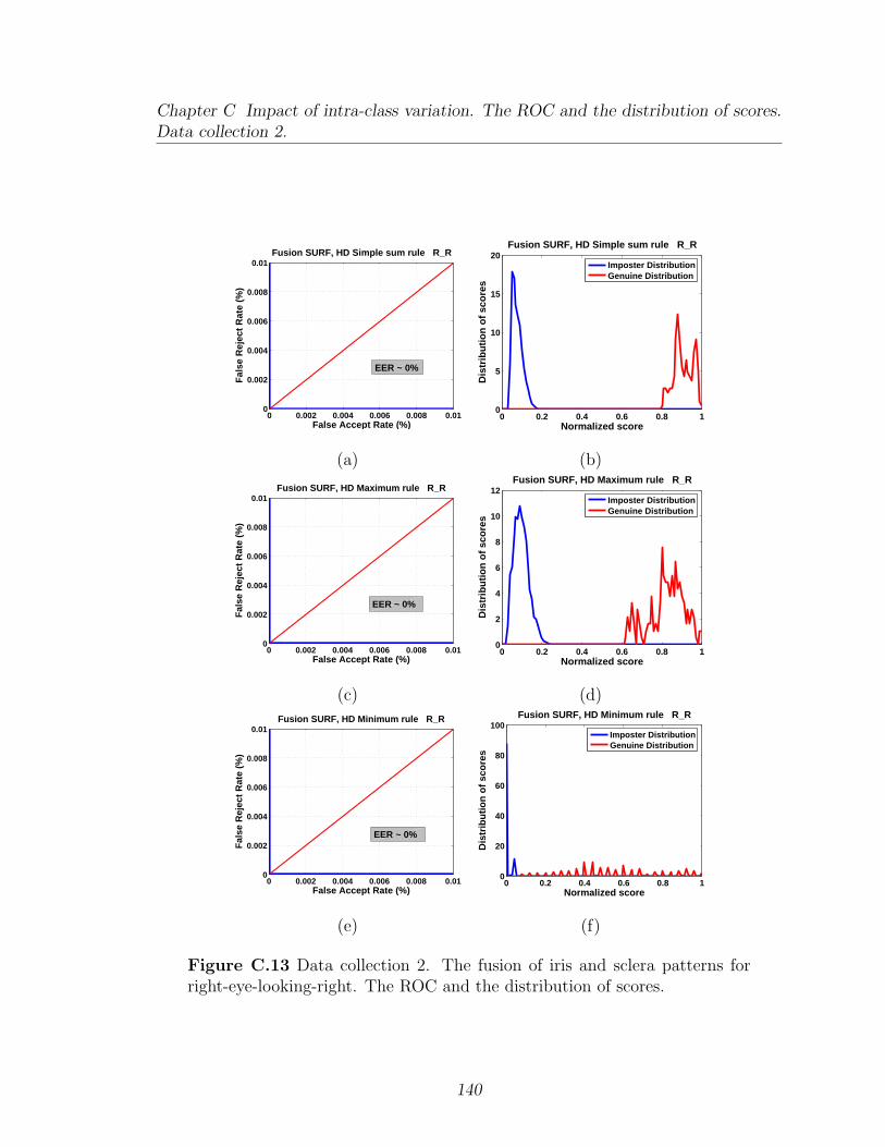
Chapter C Impact of intra-class variation. The ROC and the distribution of scores.Data collection 2.
0 0.002 0.004 0.006 0.008 0.010
0.002
0.004
0.006
0.008
0.01Fusion SURF, HD Simple sum rule R_R
False Accept Rate (%)
Fal
se R
ejec
t R
ate
(%)
EER ~ 0%
0 0.2 0.4 0.6 0.8 10
5
10
15
20
Normalized score
Dis
trib
uti
on
of
sco
res
Fusion SURF, HD Simple sum rule R_R
Imposter DistributionGenuine Distribution
(a) (b)
0 0.002 0.004 0.006 0.008 0.010
0.002
0.004
0.006
0.008
0.01Fusion SURF, HD Maximum rule R_R
False Accept Rate (%)
Fal
se R
ejec
t R
ate
(%)
EER ~ 0%
0 0.2 0.4 0.6 0.8 10
2
4
6
8
10
12
Normalized score
Dis
trib
uti
on
of
sco
res
Fusion SURF, HD Maximum rule R_R
Imposter DistributionGenuine Distribution
(c) (d)
0 0.002 0.004 0.006 0.008 0.010
0.002
0.004
0.006
0.008
0.01Fusion SURF, HD Minimum rule R_R
False Accept Rate (%)
Fal
se R
ejec
t R
ate
(%)
EER ~ 0%
0 0.2 0.4 0.6 0.8 10
20
40
60
80
100
Normalized score
Dis
trib
uti
on
of
sco
res
Fusion SURF, HD Minimum rule R_R
Imposter DistributionGenuine Distribution
(e) (f)
Figure C.13 Data collection 2. The fusion of iris and sclera patterns forright-eye-looking-right. The ROC and the distribution of scores.
140

Bibliography
[1] I. W. Selenick, “The Double-Density Dual-Tree DWT,” IEEE Transactions on
Signal Processing 52, 1304–1314 (2004).
[2] A. Jain, A. Ross, and S. Prabhakar, “An Introduction to Biometric Recogni-
tion,” IEEE Transactions on Circuits and Systems for Video Technology 14,
4–20 (2004).
[3] A. Jain, R. Bolle, and S. Pankanti, in Biometrics personal Identification in Net-
worked Society (Kluwer Academic, 2001), Chap. Retina Identification by Robert
Hill, pp. 123–141.
[4] J. Daugman, “How Iris Recognition Works,” IEEE Transactions on Circuit and
Systems for Video Technology 14, 21–30 (2004).
[5] J. G. Daugman, “The importance of being random: statistical principles of iris
recognition,” Pattern Recognition 36, 279291 (2003).
[6] J. Daugman, “NewMethods in Iris Recognition,” IEEE Transactions on Systems,
Man, and Cybernetics- Part B, Cybernetics 37, 1167–1175 (2007).
[7] A. Ross, “Iris Recognition: The Path Forward,” IEEE Computer pp. 30–35
(2010).
141
BIBLIOGRAPHY
[8] K. W. Bowyer, K. Hollingsworth, and P. J. Flynn, “Image understanding for iris
biometrics: A survey,” Computer Vision and Image Understanding 110, 281–307
(2008).
[9] M. S. Hosseini, B. N. Araabi, and H. Soltanian-Zadeh, “Pigment Melanin: Pat-
tern for Iris Recognition,” IEEE Transactions on Instrumentation and Measure-
ment 59, 792804 (2010).
[10] A. Muron and J. Pospisil, “The human iris structure and its usages,” Acta Univ.
Palacki. Olomuc. Fac. Rerum Nat. Phys. 39, 87–95 (2000).
[11] H. Borgen, P. Bours, and S.D.Wolthusen, “Visible-Spectrum Biometric retina
Recognition,” International Conference on Intelligent Information Hiding and
Multimedia Signal Processing pp. 1056–1062 (2008).
[12] M. A. Amin and H. Yan, “Phase congruency based retinal vessel segmentation,”
Machine Learning and Cybernetics 4, 2458–2462 (2009).
[13] U. Park, R. Jillela, A. Ross, and A. K. Jain, “Periocular Biometrics in the Visible
Spectrum,” IEEE Transactions on Information Forensics and Security (TIFS) 6,
96–106 (2011).
[14] D. Woodard, S. Pundlik, P. Miller, R. Jillela, and A. Ross, “On the Use of Perioc-
ular and Iris Biometrics in Non-ideal Imagery,” Proc. of International Conference
on Pattern Recognition (ICPR) pp. 201–204 (2010), , Istanbul, Turkey.
[15] P. E. Miller, A. W. Rawls, S. J. Pundlik, and D. L. Woodard, “Personal Identi-
fication using Periocular Skin Texture,” Proceedings ACM 25th Symp. applied
Computing pp. 1496–1500 (2010), aCM Press.
142

BIBLIOGRAPHY
[16] K. Trier, in Advances in organ biology. The biology of the eye (Elsevier Inc, 2006),
Vol. 10, Chap. The Sclera, pp. 353–373.
[17] J. J. Kanski, Clinical Ophthalmology: A Systematic Approach (Elsevier Science
Limited, 2003).
[18] G. Heath, “The episclera, sclera and conjunctiva,” Optometry today. Differential
Diagnosis of Ocular Disease 9, 36–42 (2006).
[19] C. G. Owen, R. S. B. Newsom, A. R. Rudnicka, T. J. Ellis, and E. G. Woodward,
“Vascular Response of the Bulbar Conjunctiva to Diabetes and Elevated Blood
Pressure,” Ophthalmology 112, 1801–1808 (2005).
[20] C. G. Owen, R. S. B. Newsom, A. R. Rudnicka, S. Barman, T. J. Ellis, and E. G.
Woodward, “Diabetes and the Tortuosity of Vessels of the Bulbar Conjunctiva,”
Ophthalmology 115, e27–e32 (2008).
[21] R. C. Gonzales and R. E. Woods, Digital Image Processing, 2 ed. (Tom Robbins,
Upper Saddle River, New Jersey, 07458, 2001).
[22] m. Nixon and A. Aguado, Feature Extraction and Image Processing, 2nd ed.
(Elsevier Ltd., 84 Theobald’s Road, London, WC1X 8RR, UK, 2008).
[23] A. K. Jain, Fundamentals of digital image processing, 1 ed. (Prentice Hall, Inc.,
Upper Saddle River, NJ 07458, 1989).
[24] R. Derakhshani and A. Ross, “Conjunctival Scans for Personal Identification,”
United States Patent, 7327860 (2008).
[25] N. D. Kalka, J. Zuo, N. A. Schmid, and B. Cukic, “Estimating and Fusing
Quality Factors for Iris Biometric Images,” IEEE Transactions on Systems, Man
and Cybernetics, Part A: Systems and Humans 40, 509–524 (2010).
143
BIBLIOGRAPHY
[26] B. E. Bayer, “Color imaging array,” U.S.Patent 3 971 065 (1976).
[27] S. Crihalmeanu, A. Ross, and R. Derakhshani, “Enhancement and Registration
Schemes for Matching Conjunctival Vasculature,” Proc. of International Confer-
ence on Biometrics, Alghero, Italy pp. 1240–1249 (2009).
[28] X. Li, “Demosaicing by Successive Approximation,” IEEE Transactions on Image
Processing 14, 370–379 (2005).
[29] I. W. Selenick, “A New Complex-Directional Wavelet Transform and its Appli-
cation to Image Denoising,” IEEE International Conference on Image Processing
3, 573–576 (2002).
[30] I. W. Selenick, in Wavelets in Signal And Image Analysis: from Theory to Prac-
tice (Kluwer Academic Publishers, 2001), Chap. The double density DWT, pp.
39–69.
[31] C. J. Tucker, “Red and Photographic Infrared Linear Combinations for Moni-
toring Vegetation,” Remote Sensing Environment 8, 127–150 (1979).
[32] H. Proenca, “Iris Recognition: On the Segmentation of Degraded Images Ac-
quired in the Visible Wavelength,” IEEE Transaction on Pattern Analysis and
Machine Intelligence 32, 1502–1516 (2010).
[33] L. Qiang, S. Shusuke, and D. Kunio, “Selective Enhancement Filters for Nodules,
Vessels, and Airway Walls in Two or Three Dimentional CT Scans,” Medical
Physics 30 (2003).
[34] S. Periaswamy and H. Farid, “Elastic Registration in the Presence of Inten-
sity Variations,” IEEE Transactions on Medical Imaging 22, 865–874 (2003),
http://www.cs.dartmouth.edu/farid/research/registration.html.
144
BIBLIOGRAPHY
[35] H. Bay, A. Ess, T. Tuyleraars, and L. V. Gool, “Speeded-Up Robust Features,”
Computer Vision and Image Understanding (CVIU) 110, 346–359 (2008).
[36] P. A. Viola and M. J. Jones, “Rapid object detection using a boosted cascade of
simple features,” Computer Vision and Pattern Recognition pp. 511–518 (2001).
[37] A. Neubeck and L. V. Gool, “Efficient non-maximum suppresion,” Proceedings
of the 18th International Conference in Pattern Recognition (ICPR) 3, 850–855
(2006).
[38] M. Brown and D. Lowe, “Invariant features from interest point groups,” British
Machine Vision Conference pp. 656–665 (2002).
[39] D. Maltoni, D. Maio, A. Jain, and S. Prabhakar, Handbook of fingerprint recog-
nition, 1 ed. (Springer Science + Business Media, Inc., 233 Spring Street, New
York, NY 10013, USA, 2003).
[40] E. M. Perez, A. D. Hughes, A. V. Stanton, S. A. Tom, A. A. Bharath, and K. H.
Parker, “Segmentation of Retinal Blood Vessels Based on the Second Directional
Derivative and Region Growing,” International Conference on Image Processing
(ICIP) 2, 173–176 (1999).
[41] Z. Wang and A. C. Bovik, “Mean Squared Error: Love It or Leave It?,” IEEE
Signal Processing Magazine pp. 98–117 (2009).
[42] M. Sonka and J. M. Fitzpatrick, in Handbook of Medical Imaging. Medical Im-
age Processing and Analysis (The International Society for Optical Engineering
(SPIE), 2004), Vol. 2, Chap. Image registration, pp. 487–497.
145
BIBLIOGRAPHY
[43] F. Maes, A. Collignon, D. Vandermeulen, G. Marchal, and P. Suetens, “Mul-
timodality Image Registration by maximization of Mutual Information,” IEEE
Transactions on Medical Imaging 16, 187–198 (1997).
[44] Z. Wang, A. C. Bovik, H. R. Sheikh, and E. P. Simoncelli, “Image Quality Assess-
ment: From Error Measurement to Structural Similarity,” IEEE Transactions on
Image Processing 13, 600–612 (2004).
[45] A. Ross, K. Nandakumar, and A. K. Jain, Handbook of Multibiometrics (Springer
Publishers, 2006).
[46] S. Crihalmeanu and A. Ross, “Multispectral Scleral Patterns for Ocular Biomet-
ric Recognition,” Pattern Recognition Letters (BIOCON) (2012), accepted / To
appear in 2012.
[47] I. Guarneri, M. Guarnera, G. Messina, and V. Tomaselli, “A signature analysis
based method for elliptical shape,” Proc. SPIE 7537 (2010).
[48] S. Crihalmeanu and A. Ross, “On the Use of Multispectral Conjunctival Vascu-
lature as a Soft Biometric,” IEEE Workshop on Applications of Computer Vision
(WACV) pp. 204–211 (2011).
[49] C. Boyce, A. Ross, M. Monaco, L. Hornak, and X. Li, “Multispectral Iris Analy-
sis: A Preliminary Study,” Proceedings of Computer Vision and Pattern Recog-
nition Workshop on Biometrics (CVPRW) (2006).
[50] X. Li, “Modeling Intra-class Variation for Non-ideal Iris Recognition,” In In
Springer LNCS 3832: Int. Conf. on Biometrics, pp. 419–427 (2006).
[51] J. R. Movellan, “Tutorial on Gabor Filters,” Technical Report pp. 1–23 (2002).
146
BIBLIOGRAPHY
[52] R. T. Tan, K. Nishino, and K. Ikeuchi, “Illumination Chromaticity Estima-
tion using Inverse-Intensity Chromaticity Space,” Computer Vision and Pattern
Recognition 1, 673–680 (2003).
[53] R. T. Tan and K. Ikeuchi, “Separating Reflection Components of Textured Sur-
faces using a Single Image,” IEEE PAMI 27, 178–193 (2005).
[54] D. Stoyanov and G. Z. Yang, “Removing Specular Reflection Components for
Robotic Assisted Laparoscopic Surgery,” IEEE International Conference in Im-
age Processing 3, 632–635 (2005).
[55] J. B. Park, “Detection of Specular Highlights in Color Images using a New Color
Space Transformation,” International Conference on Robotics and Biomimetics
(ICRB) pp. 737–741 (2004).
[56] K. Zuiderveld, in Contrast limited adaptive histogram equalization. (Academic
Press Professional, San Diego, CA, USA, 1994), Chap. In P. S. Heckbert, Graph-
ics gems IV, pp. 474–485.
[57] M. Mirmehdi, X. Xie, and J. Suri, Handbook of Texture Anlysis, 1 ed. (Imperial
College Press, 57 Shelton Street, Covent Garden, London WC2H 9HE, 2008).
147