Multispectral and Hyperspectral Image Fusion by MS/HS...
10
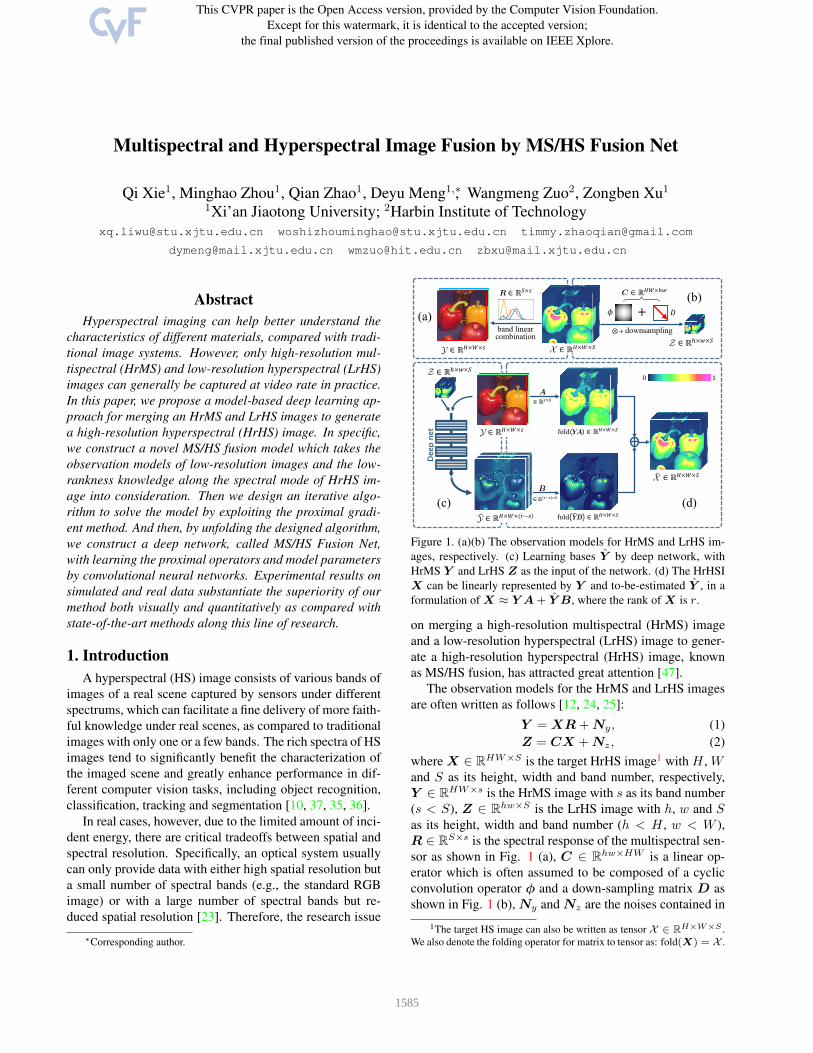
Multispectral and Hyperspectral Image Fusion by MS/HS Fusion Net Qi Xie 1 , Minghao Zhou 1 , Qian Zhao 1 , Deyu Meng 1, * , Wangmeng Zuo 2 , Zongben Xu 1 1 Xi’an Jiaotong University; 2 Harbin Institute of Technology [email protected] [email protected] [email protected] [email protected] [email protected] [email protected] Abstract Hyperspectral imaging can help better understand the characteristics of different materials, compared with tradi- tional image systems. However, only high-resolution mul- tispectral (HrMS) and low-resolution hyperspectral (LrHS) images can generally be captured at video rate in practice. In this paper, we propose a model-based deep learning ap- proach for merging an HrMS and LrHS images to generate a high-resolution hyperspectral (HrHS) image. In specific, we construct a novel MS/HS fusion model which takes the observation models of low-resolution images and the low- rankness knowledge along the spectral mode of HrHS im- age into consideration. Then we design an iterative algo- rithm to solve the model by exploiting the proximal gradi- ent method. And then, by unfolding the designed algorithm, we construct a deep network, called MS/HS Fusion Net, with learning the proximal operators and model parameters by convolutional neural networks. Experimental results on simulated and real data substantiate the superiority of our method both visually and quantitatively as compared with state-of-the-art methods along this line of research. 1. Introduction A hyperspectral (HS) image consists of various bands of images of a real scene captured by sensors under different spectrums, which can facilitate a fine delivery of more faith- ful knowledge under real scenes, as compared to traditional images with only one or a few bands. The rich spectra of HS images tend to significantly benefit the characterization of the imaged scene and greatly enhance performance in dif- ferent computer vision tasks, including object recognition, classification, tracking and segmentation [10, 37, 35, 36]. In real cases, however, due to the limited amount of inci- dent energy, there are critical tradeoffs between spatial and spectral resolution. Specifically, an optical system usually can only provide data with either high spatial resolution but a small number of spectral bands (e.g., the standard RGB image) or with a large number of spectral bands but re- duced spatial resolution [23]. Therefore, the research issue * Corresponding author. + Z Z X Y R Deep net ∈ℝ × × × ∈ℝ × fold ∈ℝ × × ∈ℝ × (c) (d) ℝ − × ∈ ∈ℝ × ×( − ) fold ∈ℝ × × × ∈ℝ × ∈ℝ × × (a) (b) ⊗+ downsampling band linear combination ∈ ℝ × Y Y X A YA YB B ∈ℝ × C Figure 1. (a)(b) The observation models for HrMS and LrHS im- ages, respectively. (c) Learning bases ˆ Y by deep network, with HrMS Y and LrHS Z as the input of the network. (d) The HrHSI X can be linearly represented by Y and to-be-estimated ˆ Y , in a formulation of X ≈ YA + ˆ YB, where the rank of X is r. on merging a high-resolution multispectral (HrMS) image and a low-resolution hyperspectral (LrHS) image to gener- ate a high-resolution hyperspectral (HrHS) image, known as MS/HS fusion, has attracted great attention [47]. The observation models for the HrMS and LrHS images are often written as follows [12, 24, 25]: Y = XR + N y , (1) Z = CX + N z , (2) where X ∈ R HW×S is the target HrHS image 1 with H, W and S as its height, width and band number, respectively, Y ∈ R HW×s is the HrMS image with s as its band number (s<S), Z ∈ R hw×S is the LrHS image with h, w and S as its height, width and band number (h<H, w<W ), R ∈ R S×s is the spectral response of the multispectral sen- sor as shown in Fig. 1 (a), C ∈ R hw×HW is a linear op- erator which is often assumed to be composed of a cyclic convolution operator φ and a down-sampling matrix D as shown in Fig. 1 (b), N y and N z are the noises contained in 1 The target HS image can also be written as tensor X∈ R H×W×S . We also denote the folding operator for matrix to tensor as: fold(X)= X . 1585
Transcript of Multispectral and Hyperspectral Image Fusion by MS/HS...
Multispectral and Hyperspectral Image Fusion by MS/HS Fusion Net
Qi Xie1, Minghao Zhou1, Qian Zhao1, Deyu Meng1,∗, Wangmeng Zuo2, Zongben Xu1
1Xi’an Jiaotong University; 2Harbin Institute of Technology
[email protected] [email protected] [email protected]
[email protected] [email protected] [email protected]
Abstract
Hyperspectral imaging can help better understand the
characteristics of different materials, compared with tradi-
tional image systems. However, only high-resolution mul-
tispectral (HrMS) and low-resolution hyperspectral (LrHS)
images can generally be captured at video rate in practice.
In this paper, we propose a model-based deep learning ap-
proach for merging an HrMS and LrHS images to generate
a high-resolution hyperspectral (HrHS) image. In specific,
we construct a novel MS/HS fusion model which takes the
observation models of low-resolution images and the low-
rankness knowledge along the spectral mode of HrHS im-
age into consideration. Then we design an iterative algo-
rithm to solve the model by exploiting the proximal gradi-
ent method. And then, by unfolding the designed algorithm,
we construct a deep network, called MS/HS Fusion Net,
with learning the proximal operators and model parameters
by convolutional neural networks. Experimental results on
simulated and real data substantiate the superiority of our
method both visually and quantitatively as compared with
state-of-the-art methods along this line of research.
1. Introduction
A hyperspectral (HS) image consists of various bands of
images of a real scene captured by sensors under different
spectrums, which can facilitate a fine delivery of more faith-
ful knowledge under real scenes, as compared to traditional
images with only one or a few bands. The rich spectra of HS
images tend to significantly benefit the characterization of
the imaged scene and greatly enhance performance in dif-
ferent computer vision tasks, including object recognition,
classification, tracking and segmentation [10, 37, 35, 36].
In real cases, however, due to the limited amount of inci-
dent energy, there are critical tradeoffs between spatial and
spectral resolution. Specifically, an optical system usually
can only provide data with either high spatial resolution but
a small number of spectral bands (e.g., the standard RGB
image) or with a large number of spectral bands but re-
duced spatial resolution [23]. Therefore, the research issue
∗Corresponding author.
+
Z
ZXY
R
Deep
net
∈ ℝ × ×
×∈ ℝ × fold ∈ ℝ × ×
∈ ℝ ×
(c) (d)ℝ − ×∈∈ ℝ × ×( − ) fold ∈ ℝ × ×
×∈ ℝ × ∈ ℝ × ×
(a)
(b)
⊗+ downsamplingband linearcombination
∈ ℝ ×
Y
Y
X
A
YA
YB
B
∈ ℝ ×C
Figure 1. (a)(b) The observation models for HrMS and LrHS im-
ages, respectively. (c) Learning bases Y by deep network, with
HrMS Y and LrHS Z as the input of the network. (d) The HrHSI
X can be linearly represented by Y and to-be-estimated Y , in a
formulation of X ≈ Y A+ Y B, where the rank of X is r.
on merging a high-resolution multispectral (HrMS) image
and a low-resolution hyperspectral (LrHS) image to gener-
ate a high-resolution hyperspectral (HrHS) image, known
as MS/HS fusion, has attracted great attention [47].
The observation models for the HrMS and LrHS images
are often written as follows [12, 24, 25]:
Y = XR+Ny, (1)
Z = CX +Nz, (2)
where X ∈ RHW×S is the target HrHS image1 with H , W
and S as its height, width and band number, respectively,
Y ∈ RHW×s is the HrMS image with s as its band number
(s < S), Z ∈ Rhw×S is the LrHS image with h, w and S
as its height, width and band number (h < H , w < W ),
R ∈ RS×s is the spectral response of the multispectral sen-
sor as shown in Fig. 1 (a), C ∈ Rhw×HW is a linear op-
erator which is often assumed to be composed of a cyclic
convolution operator φ and a down-sampling matrix D as
shown in Fig. 1 (b), Ny and Nz are the noises contained in
1The target HS image can also be written as tensor X ∈ RH×W×S .
We also denote the folding operator for matrix to tensor as: fold(X) = X .
1585
HrMS and LrHS images, respectively. Many methods have
been designed based on (1) and (2), and achieved good per-
formance [40, 14, 24, 25].
Since directly recovering the HrHS image X is an ill-
posed inverse problem, many techniques have been ex-
ploited to recover X by assuming certain priors on it. For
example, [54, 2, 11] utilize the prior knowledge of HrHS
that its spatial information could be sparsely represented un-
der a dictionary trained from HrMS. Besides, [27] assumes
the local spatial smoothness prior on the HrHS image and
uses total variation regularization to encode it in their opti-
mization model. Instead of exploring spatial prior knowl-
edge from HrHS, [52] and [26] assume more intrinsic spec-
tral correlation prior on HrHS, and use low-rank techniques
to encode such prior along the spectrum to reduce spectral
distortions. Albeit effective for some applications, the ratio-
nality of these techniques relies on the subjective prior as-
sumptions imposed on the unknown HrHS to be recovered.
An HrHS image collected from real scenes, however, could
possess highly diverse configurations both along space and
across spectrum. Such conventional learning regimes thus
could not always flexibly adapt different HS image struc-
tures and still have room for performance improvement.
Methods based on Deep Learning (DL) have outper-
formed traditional approaches in many computer vision
tasks [34] in the past decade, and have been introduced to
HS/MS fusion problem very recently [28, 30]. As com-
pared with conventional methods, these DL based ones are
superior in that they need fewer assumptions on the prior
knowledge of the to-be-recovered HrHS, while can be di-
rectly trained on a set of paired training data simulating the
network inputs (LrHS&HrMS images) and outputs (HrHS
images). The most commonly employed network structures
include CNN [7], 3D CNN [28], and residual net [30]. Like
other image restoration tasks where DL is successfully ap-
plied to, these DL-based methods have also achieved good
resolution performance for MS/MS fusion task.
However, the current DL-based MS/HS fusion meth-
ods still have evident drawbacks. The most critical one is
that these methods use general frameworks for other tasks,
which are not specifically designed for MS/HS fusion. This
makes them lack interpretability specific to the problem.
In particular, they totally neglect the observation models
(1) and (2) [28, 30], especially the operators R and C,
which facilitate an understanding of how LrHS and HrMs
are generated from the HrHS. Such understanding, how-
ever, should be useful for calculating HrHS images. Besides
this generalization issue, current DL methods also neglect
the general prior structures of HS images, such as spectral
low-rankness. Such priors are intrinsically possessed by all
meaningful HS images, which implies that DL-based meth-
ods still have room for further enhancement.
In this paper, we propose a novel deep learning-based
method that integrates the observation models and image
prior learning into a single network architecture. This work
mainly contains the following three-fold contributions:
Firstly, we propose a novel MS/HS fusion model, which
not only takes the observation models (1) and (2) into con-
sideration but also exploits the approximate low-rankness
prior structure along the spectral mode of the HrHS im-
age to reduce spectral distortions [52, 26]. Specifically, we
prove that if and only if observation model (1) can be sat-
isfied, the matrix of HrHS image X can be linearly rep-
resented by the columns in HrMS matrix Y and a to-be-
estimated matrix Y , i.e., X = Y A+ Y B with coefficient
matrices A and B. One can see Fig. 1 (d) for easy under-
standing. We then construct a concise model by combining
the observation model (2) and the linear representation of
X . We also exploit the proximal gradient method [3] to
design an iterative algorithm to solve the proposed model.
Secondly, we unfold this iterative algorithm into a deep
network architecture, called MS/HS Fusion Net or MHF-
net, to implicitly learn the to-be-estimated Y , as shown in
Fig. 1 (c). After obtaining Y , we can then easily achieve X
with Y and Y . To the best of our knowledge, this is the first
deep-learning-based MS/HS fusion method that fully con-
siders the intrinsic mechanism of the MS/HS fusion prob-
lem. Moreover, all the parameters involved in the model can
be automatically learned from training data in an end-to-end
manner. This means that the spatial and spectral responses
(R and C) no longer need to be estimated beforehand as
most of the traditional non-DL methods did, nor to be fully
neglected as current DL methods did.
Thirdly, we have collected or realized current state-of-
the-art algorithms for the investigated MS/HS fusion task,
and compared their performance on a series of synthetic and
real problems. The experimental results comprehensively
substantiate the superiority of the proposed method, both
quantitatively and visually.
In this paper, we denote scalar, vector, matrix and ten-
sor in non-bold case, bold lower case, bold upper case and
calligraphic upper case letters, respectively.
2. Related work
2.1. Traditional methods
The pansharpening technique in remote sensing is
closely related to the investigated MS/HS problem. This
task aims to obtain a high spatial resolution MS image by
the fusion of a MS image and a wide-band panchromatic
image. A heuristic approach to perform MS/HS fusion is to
treat it as a number of pansharpening sub-problems, where
each band of the HrMS image plays the role of a panchro-
matic image. There are mainly two categories of pansharp-
ening methods: component substitution (CS) [5, 17, 1] and
multiresolution analysis (MRA) [20, 21, 4, 33, 6]. These
methods always suffer from the high spectral distortion,
1586
since a single panchromatic image contains little spectral
information as compared with the expected HS image.
In the last few years, machine learning based meth-
ods have gained much attention on MS/HS fusion problem
[54, 2, 11, 14, 52, 48, 26, 40]. Some of these methods used
sparse coding technique to learn a dictionary on the patches
across a HrMS image, which delivers spatial knowledge of
HrHS to a certain extent, and then learn a coefficient ma-
trix from LrHS to fully represent the HrHS [54, 2, 11, 40].
Some other methods, such as [14], use the sparse matrix fac-
torization to learn a spectral dictionary for LrHS images and
then construct HrMS images by exploiting both the spectral
dictionary and HrMS images. The low-rankness of HS im-
ages can also be exploited with non-negative matrix factor-
ization, which helps to reduce spectral distortions and en-
hances the MS/HS fusion performance [52, 48, 26]. The
main drawback of these methods is that they are mainly de-
signed based on human observations and strong prior as-
sumptions, which may not be very accurate and would not
always hold for diverse real world images.
2.2. Deep learning based methods
Recently, a number of DL-based pansharpening meth-
ods were proposed by exploiting different network struc-
tures [15, 22, 42, 43, 29, 30, 32]. These methods can be
easily adapted to MS/HS fusion problem. For example,
very recently, [28] proposed a 3D-CNN based MS/HS fu-
sion method by using PCA to reduce the computational
cost. This method is usually trained with prepared train-
ing data. The network inputs are set as the combination
of HrMS/panchromatic images and LrHS/multispectral im-
ages (which is usually interpolated to the same spatial size
as HrMS/panchromatic images in advance), and the outputs
are the corresponding HrHS images. The current DL-based
methods have been verified to be able to attain good per-
formance. They, however, just employ networks assembled
with some off-the-shelf components in current deep learn-
ing toolkits, which are not specifically designed against the
investigated problem. Thus the main drawback of this tech-
nique is the lack of interpretability to this particular MS/HS
fusion task. In specific, both the intrinsic observation model
(1), (2) and the evident prior structures, like the spectral cor-
relation property, possessed by HS images have been ne-
glected by such kinds of “black-box” deep model.
3. MS/HS fusion model
In this section, we demonstrate the proposed MS/HS fu-
sion model in detail.
3.1. Model formulation
We first introduce an equivalent formulation for observa-
tion model (1). Specifically, we have following theorem2.
2All proofs are presented in supplementary material.
Theorem 1. For any X ∈ RHW×S and Y ∈ R
HW×s, if
rank(X) = r > s and rank(Y ) = s, then the following two
statements are equivalent to each other:
(a) There exists an R ∈ RS×s, subject to,
Y = XR. (3)
(b) There exist A ∈ Rs×S , B ∈ R
(r−s)×S and Y ∈R
HW×(r−s), subject to,
X = Y A+ Y B. (4)
In reality, the band number of an HrMS image is usually
not large, which makes it full rank along spectral mode. For
example, the most commonly used HrMS images, RGB im-
ages, contain three bands, and their rank along the spectral
mode is usually also three. Thus, by letting Y = Y −Ny
where Y is the observed HrMS in (1), it is easy to find that
Y and X satisfy the conditions in Theorem 1. Then the
observation model (1) is equivalent3 to
X = Y A+ Y B +Nx, (5)
where Nx = −NyA is caused by the noise contained in the
HrMS image. In (5), [Y , Y ] can be viewed as r bases that
represent columns in X with coefficients matrix [A;B] ∈
Rr×S , where only the r − s bases in Y are unknown. In
addition, we can derive the following corollary:
Corollary 1. For any Y ∈ RHW×s, Z ∈ R
hw×S , C ∈Rhw×HW , if rank(Y ) = s and rank(Z) = r > s, then the
following two statements are equivalent to each other:
(a) There exist X ∈ RHW×S and R ∈ R
S×s, subject to,
Y = XR, Z = CX, rank(X) = r. (6)
(b) There exist A ∈ Rs×S , r > s, B ∈ R
(r−s)×S and
Y ∈ RHW×(r−s), subject to,
Z = C(
Y A+ Y B)
. (7)
Let Z = Z −Nz , where Z is the observed LrHS image
in (2). It is easy to find that, when being viewed as equations
of the to-be-estimated X , R and C, the observation model
(1) and model (2) are equivalent to the following equation
of Y , A, B and C:
Z = C(
Y A+ Y B)
+N , (8)
where N = Nz − CNyA denotes the noise contained in
HrMS and LrHS image. Then, we can design the following
MS/HS fusion model:
minY
∥
∥
∥C
(
Y A+ Y B)
−Z
∥
∥
∥
2
F+ λf
(
Y)
, (9)
3We say two equation are equivalent to each other if the solution of
one equation can easily achieve by solving the other one
1587
where λ is a trade-off parameter, and f(·) is a regularization
function. We adopt regularization on the to-be-estimated
bases in Y , rather than on X as in conventional, to facil-
itate an entire preservation of spatial details4 contained in
the known HrMS bases (Y ) for representing X .
It should be noted that for data obtained with the same
sensors, A, B and C are fixed. This means that they can be
learned from the training data. In the later sections we will
show how to learn them with a deep network.
3.2. Model optimization
We now solve (9) using a proximal gradient algorithm
[3], which iteratively updates Y by calculating
Y (k+1) = argminY
Q(
Y , Y (k))
, (10)
where Y (k) is the updating result after k−1 iterations, k =1, 2, · · · ,K, and Q(Y , Y (k)) is a quadratic approximation
[3] defined as:
Q(
Y , Y (k))
=g(
Y (k))
+⟨
Y − Y (k),∇g(
Y (k))⟩
+1
2η
∥
∥
∥Y − Y (k)
∥
∥
∥
2
F+ λf
(
Y)
,(11)
where g(Y (k)) = ‖C(Y A+ Y (k)B)− Z‖2F and η plays
the role of stepsize.
It is easy to prove that the problem (10) is equivalent to:
minY
1
2
∥
∥
∥Y −
(
Y (k)−η∇g(
Y (k)))
∥
∥
∥
2
F+ληf
(
Y)
. (12)
For many kinds of regularization terms, the solution of Eq.
(12) is usually in closed-form [8], written as:
Y (k+1) = proxλη
(
Y (k)−η∇g(
Y (k)))
, (13)
where proxλη(·) is a proximal operator dependent on f(·).
Since ∇g(Y (k)) = CT (C(Y A + Y (k)B) − Z)BT , we
can obtain the final updating rule for Y :
Y(k+1)=proxλη
(
Y(k)
−ηCT(
C
(
YA+ Y(k)B
)
−Z
)
BT)
.
(14)
We can then unfold this algorithm into a deep network.
4. MS/HS fusion net
Based on the above algorithm, we build a deep neural
network for MS/HS fusion by unfolding all steps of the al-
gorithm as network layers. This technique has been widely
utilized in various computer vision tasks and has been sub-
stantiated to be effective in compressed sensing, dehazing,
deconvolution, etc. [44, 45, 53]. The proposed network is a
4 Directly imposing regularization terms on X , e.g., TV norm, will
lead to losing of details like the sharp edge and lines in X .
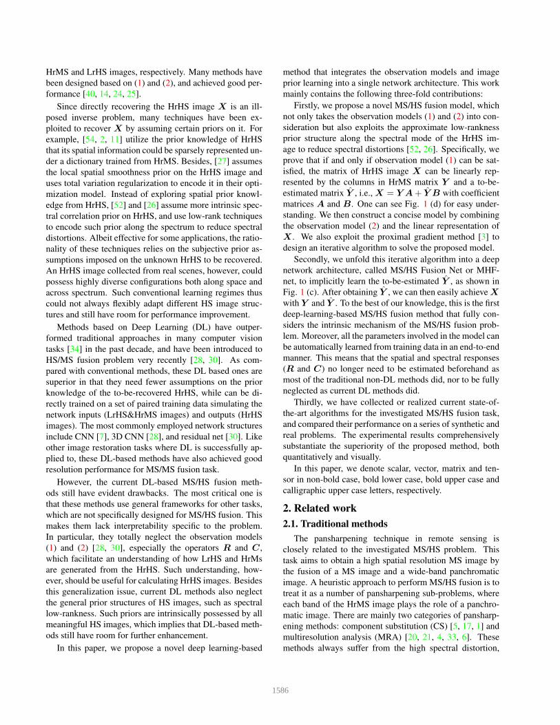
For 𝑘𝑘 = 1:𝐾𝐾 do: In stage 𝑘𝑘 = 1:𝐾𝐾 of the network do:
Iterative optimization algorithm Network design
𝒳𝒳 𝑘𝑘 = 𝒴𝒴 ×3 𝑨𝑨𝑻𝑻 + �𝒴𝒴(𝑘𝑘) ×3 𝑩𝑩𝑻𝑻𝑿𝑿 𝑘𝑘 = 𝒀𝒀𝑨𝑨+ �𝒀𝒀(𝑘𝑘)𝑩𝑩 ℰ 𝑘𝑘 = downSample𝜃𝜃𝑑𝑑𝑘𝑘 𝒳𝒳 𝑘𝑘 − 𝒵𝒵𝑬𝑬(𝑘𝑘) = 𝑪𝑪𝑿𝑿 𝑘𝑘 − 𝒁𝒁 𝒢𝒢 𝑘𝑘 = 𝜂𝜂 ⋅ upSample𝜃𝜃𝑑𝑑𝑘𝑘 ℰ 𝑘𝑘 ×3 𝑩𝑩𝑮𝑮 𝑘𝑘 = 𝜂𝜂𝑪𝑪𝑇𝑇𝑬𝑬(𝑘𝑘)𝑩𝑩𝑇𝑇 �𝒴𝒴 𝑘𝑘+1 = proxNet𝜃𝜃𝑝𝑝𝑘𝑘 �𝒴𝒴 𝑘𝑘 − 𝒢𝒢 𝑘𝑘𝒀𝒀 𝑘𝑘+1 = prox𝜆𝜆𝜆𝜆 �𝒀𝒀(𝑘𝑘) − 𝑮𝑮 𝒌𝒌Figure 2. An illustration of relationship between the algorithm
with matrix form and the network structure with tensor form.
structure of K stages, corresponding to K iterations in the
iterative algorithm for solving Eq. (9), as shown in Fig. 3
(a) and (b). Each stage takes the HrMS image Y , LrHS im-
age Z, and the output of the previous stage Y , as inputs,
and outputs an updated Y to be the input of next layer.
4.1. Network design
Algorithm unfolding. We first decompose the updating
rule (14) into the following equivalent four sequential parts:
X(k) = Y A+ Y (k)B, (15)
E(k) = CX(k) −Z, (16)
G(k) = ηCTE(k)BT , (17)
Y (k+1) = proxλη
(
Y (k) −G(k))
. (18)
In the network framework, we use the images with their
tensor formulations (X ∈ RH×W×S , Y ∈ R
H×W×s and
Z ∈ Rh×w×S) instead of their matrix forms to protect their
spatial structure knowledge and make the network structure
(in tensor form) easily designed. We then design a network
to approximately perform the above operations in tensor
version. Refer to Fig. 2 for easy understanding.
In tensor version, Eq. (15) can be easily performed by
the two multiplications between a tensor and a matrix along
the 3rd mode of the tensor. Specifically, in the TensorFlow5
framework, multiplying a tensor with an matrix in Rm×n
along the channel mode can be easily performed by using
the 2D convolution function with a associated 1×1×m×n
tensor. Thus, we can perform the tensor version of (15) by:
X (k) = Y ×3 AT + Y(k) ×3 B
T , (19)
where ×3 denotes the mode-3 multiplication for tensor6.
In Eq. (16), the matrix C represents the spatial down-
sampling operator, which can be decomposed into 2D con-
volutions and down-sampling operators [12, 24, 25]. Thus,
we perform the tensor version of (16) by:
E(k) = downSampleθ(k)d
(
X (k))
−Z, (20)
5https://tensorflow.google.cn/6For a tensor U ∈ R
I×J×K with uijk as its elements, and V ∈
RK×L with vkl as its elements, let W = U ×3V , the elements of W are
wijl =∑K
k=1 uijkvlk . Besides, W = U ×3 V ⇔ W = UVT .
1588
AT
+−
+1)
+
+
+− +−
X (k)E(k)
G(k) Y (k
Z
(d)
(c)
×3Y Y
×3 X (k)BY (k) Y (k)
Y X (1)
E(1)
G(1) Y (2)×3Y A
X (1)
Z
+
+
+− Lo
ss F
un
ctio
n
Y
X (K)×3BY (K)Y (K)
E (K)X (k
X
(e)
(b)X
(a)
ZY
ZY
ZY
ZY
Z
A
B B
A
B
A TB
T T
T
T
T
X (k) = Y ×3AT+ Y(k)×3B
T
G(k) = η · upSampleθ(k)u
(
E(k))
×3 B
E(k) = downSampleθ(k)d
X (k)( )
−Z
Y(k+1) = proxNetθ(k)p
(
Y(k) − G(k))
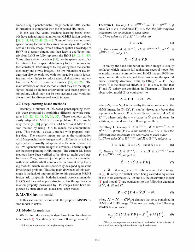
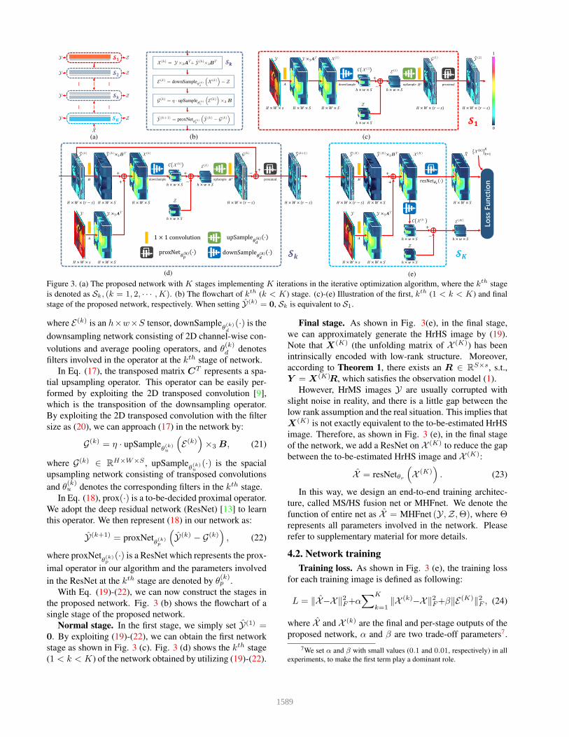
Figure 3. (a) The proposed network with K stages implementing K iterations in the iterative optimization algorithm, where the kth stage
is denoted as Sk, (k = 1, 2, · · · ,K). (b) The flowchart of kth (k < K) stage. (c)-(e) Illustration of the first, kth (1 < k < K) and final
stage of the proposed network, respectively. When setting Y(k) = 0, Sk is equivalent to S1.
where E(k) is an h×w×S tensor, downSampleθ(k)d
(·) is the
downsampling network consisting of 2D channel-wise con-
volutions and average pooling operators, and θ(k)d denotes
filters involved in the operator at the kth stage of network.
In Eq. (17), the transposed matrix CT represents a spa-
tial upsampling operator. This operator can be easily per-
formed by exploiting the 2D transposed convolution [9],
which is the transposition of the downsampling operator.
By exploiting the 2D transposed convolution with the filter
size as (20), we can approach (17) in the network by:
G(k) = η · upSampleθ(k)u
(
E(k))
×3 B, (21)
where G(k) ∈ RH×W×S , upSample
θ(k)u
(·) is the spacial
upsampling network consisting of transposed convolutions
and θ(k)u denotes the corresponding filters in the kth stage.
In Eq. (18), prox(·) is a to-be-decided proximal operator.
We adopt the deep residual network (ResNet) [13] to learn
this operator. We then represent (18) in our network as:
Y(k+1) = proxNetθ(k)p
(
Y(k) − G(k))
, (22)
where proxNetθ(k)p
(·) is a ResNet which represents the prox-
imal operator in our algorithm and the parameters involved
in the ResNet at the kth stage are denoted by θ(k)p .
With Eq. (19)-(22), we can now construct the stages in
the proposed network. Fig. 3 (b) shows the flowchart of a
single stage of the proposed network.
Normal stage. In the first stage, we simply set Y(1) =0. By exploiting (19)-(22), we can obtain the first network
stage as shown in Fig. 3 (c). Fig. 3 (d) shows the kth stage
(1 < k < K) of the network obtained by utilizing (19)-(22).
Final stage. As shown in Fig. 3(e), in the final stage,
we can approximately generate the HrHS image by (19).
Note that X(K) (the unfolding matrix of X (K)) has been
intrinsically encoded with low-rank structure. Moreover,
according to Theorem 1, there exists an R ∈ RS×s, s.t.,
Y = X(K)R, which satisfies the observation model (1).
However, HrMS images Y are usually corrupted with
slight noise in reality, and there is a little gap between the
low rank assumption and the real situation. This implies that
X(K) is not exactly equivalent to the to-be-estimated HrHS
image. Therefore, as shown in Fig. 3 (e), in the final stage
of the network, we add a ResNet on X (K) to reduce the gap
between the to-be-estimated HrHS image and X (K):
X = resNetθr
(
X (K))
. (23)
In this way, we design an end-to-end training architec-
ture, called MS/HS fusion net or MHFnet. We denote the
function of entire net as X = MHFnet (Y,Z,Θ), where Θrepresents all parameters involved in the network. Please
refer to supplementary material for more details.
4.2. Network training
Training loss. As shown in Fig. 3 (e), the training loss
for each training image is defined as following:
L = ‖X−X‖2F+α∑K
k=1‖X (k)−X‖2F+β‖E
(K)‖2F , (24)
where X and X (k) are the final and per-stage outputs of the
proposed network, α and β are two trade-off parameters7.
7We set α and β with small values (0.1 and 0.01, respectively) in all
experiments, to make the first term play a dominant role.
1589
Down
sampling
Down
sampling
X
Z
YInputsamples
Referencesamples
Training sample Training dataEstimate down sampling operator
Original data Original sample
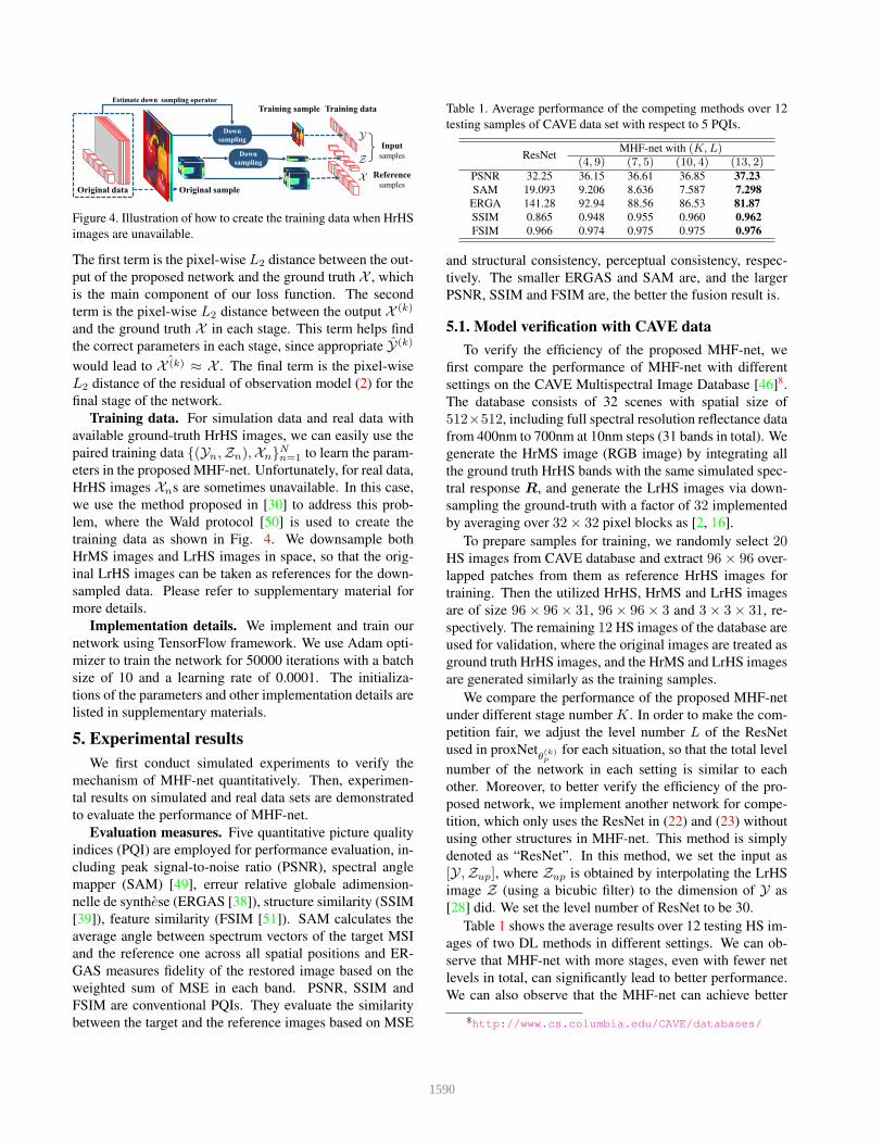
Figure 4. Illustration of how to create the training data when HrHS
images are unavailable.
The first term is the pixel-wise L2 distance between the out-
put of the proposed network and the ground truth X , which
is the main component of our loss function. The second
term is the pixel-wise L2 distance between the output X (k)
and the ground truth X in each stage. This term helps find
the correct parameters in each stage, since appropriate Y(k)
would lead to ˆX (k) ≈ X . The final term is the pixel-wise
L2 distance of the residual of observation model (2) for the
final stage of the network.
Training data. For simulation data and real data with
available ground-truth HrHS images, we can easily use the
paired training data {(Yn,Zn),Xn}Nn=1 to learn the param-
eters in the proposed MHF-net. Unfortunately, for real data,
HrHS images Xns are sometimes unavailable. In this case,
we use the method proposed in [30] to address this prob-
lem, where the Wald protocol [50] is used to create the
training data as shown in Fig. 4. We downsample both
HrMS images and LrHS images in space, so that the orig-
inal LrHS images can be taken as references for the down-
sampled data. Please refer to supplementary material for
more details.
Implementation details. We implement and train our
network using TensorFlow framework. We use Adam opti-
mizer to train the network for 50000 iterations with a batch
size of 10 and a learning rate of 0.0001. The initializa-
tions of the parameters and other implementation details are
listed in supplementary materials.
5. Experimental results
We first conduct simulated experiments to verify the
mechanism of MHF-net quantitatively. Then, experimen-
tal results on simulated and real data sets are demonstrated
to evaluate the performance of MHF-net.
Evaluation measures. Five quantitative picture quality
indices (PQI) are employed for performance evaluation, in-
cluding peak signal-to-noise ratio (PSNR), spectral angle
mapper (SAM) [49], erreur relative globale adimension-
nelle de synthese (ERGAS [38]), structure similarity (SSIM
[39]), feature similarity (FSIM [51]). SAM calculates the
average angle between spectrum vectors of the target MSI
and the reference one across all spatial positions and ER-
GAS measures fidelity of the restored image based on the
weighted sum of MSE in each band. PSNR, SSIM and
FSIM are conventional PQIs. They evaluate the similarity
between the target and the reference images based on MSE
Table 1. Average performance of the competing methods over 12
testing samples of CAVE data set with respect to 5 PQIs.
ResNetMHF-net with (K,L)
(4, 9) (7, 5) (10, 4) (13, 2)PSNR 32.25 36.15 36.61 36.85 37.23
SAM 19.093 9.206 8.636 7.587 7.298
ERGA 141.28 92.94 88.56 86.53 81.87
SSIM 0.865 0.948 0.955 0.960 0.962
FSIM 0.966 0.974 0.975 0.975 0.976
and structural consistency, perceptual consistency, respec-
tively. The smaller ERGAS and SAM are, and the larger
PSNR, SSIM and FSIM are, the better the fusion result is.
5.1. Model verification with CAVE data
To verify the efficiency of the proposed MHF-net, we
first compare the performance of MHF-net with different
settings on the CAVE Multispectral Image Database [46]8.
The database consists of 32 scenes with spatial size of
512×512, including full spectral resolution reflectance data
from 400nm to 700nm at 10nm steps (31 bands in total). We
generate the HrMS image (RGB image) by integrating all
the ground truth HrHS bands with the same simulated spec-
tral response R, and generate the LrHS images via down-
sampling the ground-truth with a factor of 32 implemented
by averaging over 32× 32 pixel blocks as [2, 16].
To prepare samples for training, we randomly select 20HS images from CAVE database and extract 96 × 96 over-
lapped patches from them as reference HrHS images for
training. Then the utilized HrHS, HrMS and LrHS images
are of size 96× 96× 31, 96× 96× 3 and 3× 3× 31, re-
spectively. The remaining 12 HS images of the database are
used for validation, where the original images are treated as
ground truth HrHS images, and the HrMS and LrHS images
are generated similarly as the training samples.
We compare the performance of the proposed MHF-net
under different stage number K. In order to make the com-
petition fair, we adjust the level number L of the ResNet
used in proxNetθ(k)p
for each situation, so that the total level
number of the network in each setting is similar to each
other. Moreover, to better verify the efficiency of the pro-
posed network, we implement another network for compe-
tition, which only uses the ResNet in (22) and (23) without
using other structures in MHF-net. This method is simply
denoted as “ResNet”. In this method, we set the input as
[Y,Zup], where Zup is obtained by interpolating the LrHS
image Z (using a bicubic filter) to the dimension of Y as
[28] did. We set the level number of ResNet to be 30.
Table 1 shows the average results over 12 testing HS im-
ages of two DL methods in different settings. We can ob-
serve that MHF-net with more stages, even with fewer net
levels in total, can significantly lead to better performance.
We can also observe that the MHF-net can achieve better
8http://www.cs.columbia.edu/CAVE/databases/
1590
(n) MHF-net
(g) GSA
(i) M-FUSE
(b) Ground truth
(j) SAMF
(c) FUSE
(m) ResNet
(f) SFIM-HS
0
1
(h) CNMF
(a) RGB & LrHS (e) GLP-HS
(l) 3D-CNN
(d) ICCV2015
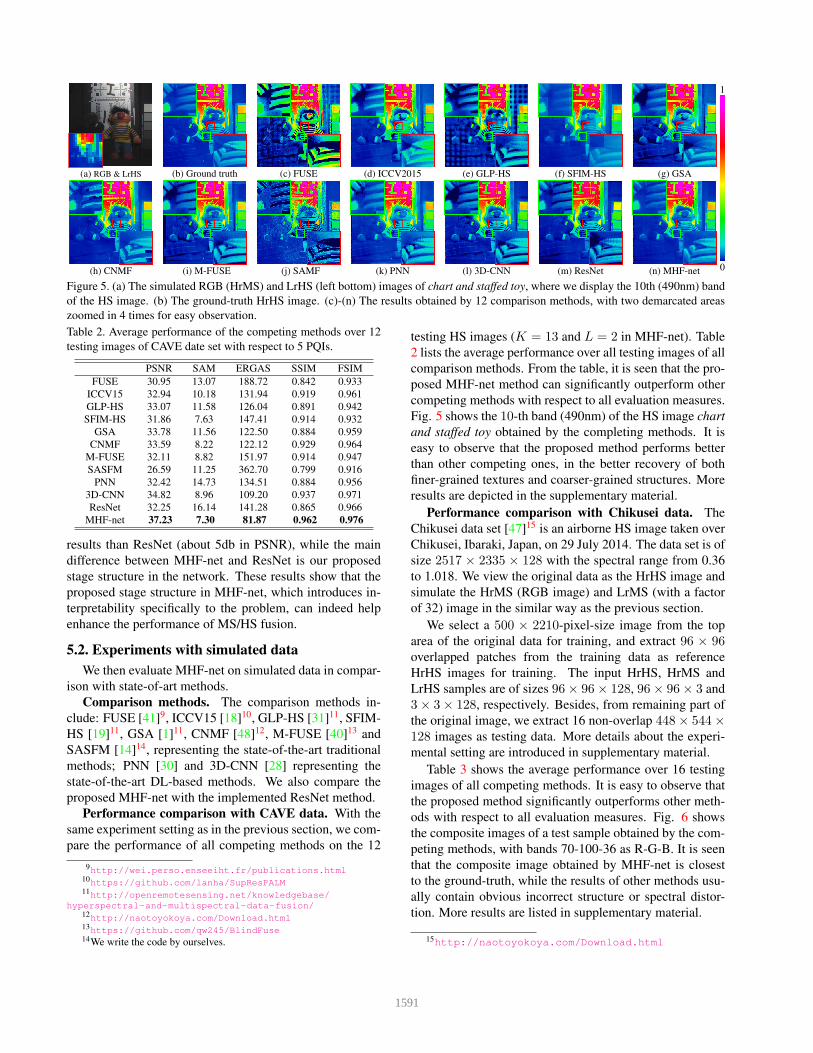
(k) PNNFigure 5. (a) The simulated RGB (HrMS) and LrHS (left bottom) images of chart and staffed toy, where we display the 10th (490nm) band
of the HS image. (b) The ground-truth HrHS image. (c)-(n) The results obtained by 12 comparison methods, with two demarcated areas
zoomed in 4 times for easy observation.
Table 2. Average performance of the competing methods over 12
testing images of CAVE date set with respect to 5 PQIs.
PSNR SAM ERGAS SSIM FSIM
FUSE 30.95 13.07 188.72 0.842 0.933
ICCV15 32.94 10.18 131.94 0.919 0.961
GLP-HS 33.07 11.58 126.04 0.891 0.942
SFIM-HS 31.86 7.63 147.41 0.914 0.932
GSA 33.78 11.56 122.50 0.884 0.959
CNMF 33.59 8.22 122.12 0.929 0.964
M-FUSE 32.11 8.82 151.97 0.914 0.947
SASFM 26.59 11.25 362.70 0.799 0.916
PNN 32.42 14.73 134.51 0.884 0.956
3D-CNN 34.82 8.96 109.20 0.937 0.971
ResNet 32.25 16.14 141.28 0.865 0.966
MHF-net 37.23 7.30 81.87 0.962 0.976
results than ResNet (about 5db in PSNR), while the main
difference between MHF-net and ResNet is our proposed
stage structure in the network. These results show that the
proposed stage structure in MHF-net, which introduces in-
terpretability specifically to the problem, can indeed help
enhance the performance of MS/HS fusion.
5.2. Experiments with simulated data
We then evaluate MHF-net on simulated data in compar-
ison with state-of-art methods.
Comparison methods. The comparison methods in-
clude: FUSE [41]9, ICCV15 [18]10, GLP-HS [31]11, SFIM-
HS [19]11, GSA [1]11, CNMF [48]12, M-FUSE [40]13 and
SASFM [14]14, representing the state-of-the-art traditional
methods; PNN [30] and 3D-CNN [28] representing the
state-of-the-art DL-based methods. We also compare the
proposed MHF-net with the implemented ResNet method.
Performance comparison with CAVE data. With the
same experiment setting as in the previous section, we com-
pare the performance of all competing methods on the 12
9http://wei.perso.enseeiht.fr/publications.html10https://github.com/lanha/SupResPALM11http://openremotesensing.net/knowledgebase/
hyperspectral-and-multispectral-data-fusion/12http://naotoyokoya.com/Download.html13https://github.com/qw245/BlindFuse14We write the code by ourselves.
testing HS images (K = 13 and L = 2 in MHF-net). Table
2 lists the average performance over all testing images of all
comparison methods. From the table, it is seen that the pro-
posed MHF-net method can significantly outperform other
competing methods with respect to all evaluation measures.
Fig. 5 shows the 10-th band (490nm) of the HS image chart
and staffed toy obtained by the completing methods. It is
easy to observe that the proposed method performs better
than other competing ones, in the better recovery of both
finer-grained textures and coarser-grained structures. More
results are depicted in the supplementary material.
Performance comparison with Chikusei data. The
Chikusei data set [47]15 is an airborne HS image taken over
Chikusei, Ibaraki, Japan, on 29 July 2014. The data set is of
size 2517 × 2335 × 128 with the spectral range from 0.36
to 1.018. We view the original data as the HrHS image and
simulate the HrMS (RGB image) and LrMS (with a factor
of 32) image in the similar way as the previous section.
We select a 500 × 2210-pixel-size image from the top
area of the original data for training, and extract 96 × 96overlapped patches from the training data as reference
HrHS images for training. The input HrHS, HrMS and
LrHS samples are of sizes 96× 96× 128, 96× 96× 3 and
3× 3× 128, respectively. Besides, from remaining part of
the original image, we extract 16 non-overlap 448× 544×128 images as testing data. More details about the experi-
mental setting are introduced in supplementary material.
Table 3 shows the average performance over 16 testing
images of all competing methods. It is easy to observe that
the proposed method significantly outperforms other meth-
ods with respect to all evaluation measures. Fig. 6 shows
the composite images of a test sample obtained by the com-
peting methods, with bands 70-100-36 as R-G-B. It is seen
that the composite image obtained by MHF-net is closest
to the ground-truth, while the results of other methods usu-
ally contain obvious incorrect structure or spectral distor-
tion. More results are listed in supplementary material.
15http://naotoyokoya.com/Download.html
1591
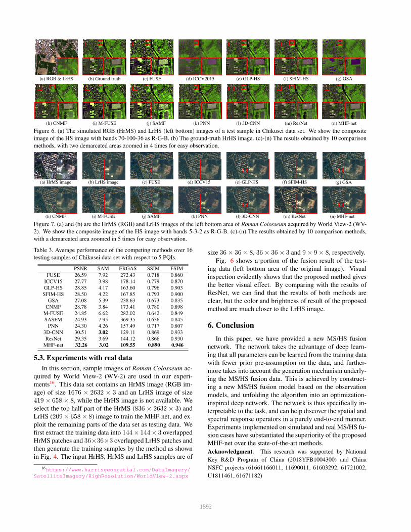
(b) Ground truth
(i) M-FUSE
(c) FUSE
(j) SAMF (m) ResNet
(f) SFIM-HS
(n) MHF-net
(g) GSA
(h) CNMF
(a) RGB & LrHS (e) GLP-HS
(l) 3D-CNN
(d) ICCV2015
(k) PNNFigure 6. (a) The simulated RGB (HrMS) and LrHS (left bottom) images of a test sample in Chikusei data set. We show the composite
image of the HS image with bands 70-100-36 as R-G-B. (b) The ground-truth HrHS image. (c)-(n) The results obtained by 10 comparison
methods, with two demarcated areas zoomed in 4 times for easy observation.
(b) LrHS image
(i) M-FUSE
(c) FUSE
(j) SAMF (m) ResNet
(f) SFIM-HS
(n) MHF-net
(g) GSA
(h) CNMF
(a) HrMS image (e) GLP-HS
(l) 3D-CNN
(d) ICCV15
(k) PNN
Figure 7. (a) and (b) are the HrMS (RGB) and LrHS images of the left bottom area of Roman Colosseum acquired by World View-2 (WV-
2). We show the composite image of the HS image with bands 5-3-2 as R-G-B. (c)-(n) The results obtained by 10 comparison methods,
with a demarcated area zoomed in 5 times for easy observation.
Table 3. Average performance of the competing methods over 16
testing samples of Chikusei data set with respect to 5 PQIs.
PSNR SAM ERGAS SSIM FSIM
FUSE 26.59 7.92 272.43 0.718 0.860
ICCV15 27.77 3.98 178.14 0.779 0.870
GLP-HS 28.85 4.17 163.60 0.796 0.903
SFIM-HS 28.50 4.22 167.85 0.793 0.900
GSA 27.08 5.39 238.63 0.673 0.835
CNMF 28.78 3.84 173.41 0.780 0.898
M-FUSE 24.85 6.62 282.02 0.642 0.849
SASFM 24.93 7.95 369.35 0.636 0.845
PNN 24.30 4.26 157.49 0.717 0.807
3D-CNN 30.51 3.02 129.11 0.869 0.933
ResNet 29.35 3.69 144.12 0.866 0.930
MHF-net 32.26 3.02 109.55 0.890 0.946
5.3. Experiments with real data
In this section, sample images of Roman Colosseum ac-
quired by World View-2 (WV-2) are used in our experi-
ments16. This data set contains an HrMS image (RGB im-
age) of size 1676 × 2632 × 3 and an LrHS image of size
419× 658× 8, while the HrHS image is not available. We
select the top half part of the HrMS (836 × 2632 × 3) and
LrHS (209× 658× 8) image to train the MHF-net, and ex-
ploit the remaining parts of the data set as testing data. We
first extract the training data into 144× 144× 3 overlapped
HrMS patches and 36×36×3 overlapped LrHS patches and
then generate the training samples by the method as shown
in Fig. 4. The input HrHS, HrMS and LrHS samples are of
16https://www.harrisgeospatial.com/DataImagery/
SatelliteImagery/HighResolution/WorldView-2.aspx
size 36× 36× 8, 36× 36× 3 and 9× 9× 8, respectively.
Fig. 6 shows a portion of the fusion result of the test-
ing data (left bottom area of the original image). Visual
inspection evidently shows that the proposed method gives
the better visual effect. By comparing with the results of
ResNet, we can find that the results of both methods are
clear, but the color and brightness of result of the proposed
method are much closer to the LrHS image.
6. Conclusion
In this paper, we have provided a new MS/HS fusion
network. The network takes the advantage of deep learn-
ing that all parameters can be learned from the training data
with fewer prior pre-assumption on the data, and further-
more takes into account the generation mechanism underly-
ing the MS/HS fusion data. This is achieved by construct-
ing a new MS/HS fusion model based on the observation
models, and unfolding the algorithm into an optimization-
inspired deep network. The network is thus specifically in-
terpretable to the task, and can help discover the spatial and
spectral response operators in a purely end-to-end manner.
Experiments implemented on simulated and real MS/HS fu-
sion cases have substantiated the superiority of the proposed
MHF-net over the state-of-the-art methods.
Acknowledgment. This research was supported by National
Key R&D Program of China (2018YFB1004300) and China
NSFC projects (61661166011, 11690011, 61603292, 61721002,
U1811461, 61671182)
1592
References
[1] B. Aiazzi, S. Baronti, and M. Selva. Improving component
substitution pansharpening through multivariate regression
of ms + pan data. IEEE Transactions on Geoscience and
Remote Sensing, 45(10):3230–3239, 2007. 2, 7
[2] N. Akhtar, F. Shafait, and A. Mian. Sparse spatio-spectral
representation for hyperspectral image super-resolution. In
European Conference on Computer Vision, pages 63–78.
Springer, 2014. 2, 3, 6
[3] A. Beck and M. Teboulle. A fast iterative shrinkage-
thresholding algorithm for linear inverse problems. SIAM
journal on imaging sciences, 2(1):183–202, 2009. 2, 4
[4] P. J. Burt and E. H. Adelson. The laplacian pyramid as a
compact image code. In Readings in Computer Vision, pages
671–679. Elsevier, 1987. 2
[5] P. Chavez, S. C. Sides, J. A. Anderson, et al. Compari-
son of three different methods to merge multiresolution and
multispectral data- landsat tm and spot panchromatic. Pho-
togrammetric Engineering and remote sensing, 57(3):295–
303, 1991. 2
[6] M. N. Do and M. Vetterli. The contourlet transform: an effi-
cient directional multiresolution image representation. IEEE
Transactions on image processing, 14(12):2091–2106, 2005.
2
[7] C. Dong, C. C. Loy, K. He, and X. Tang. Image
super-resolution using deep convolutional networks. IEEE
transactions on pattern analysis and machine intelligence,
38(2):295–307, 2016. 2
[8] D. L. Donoho. De-noising by soft-thresholding. IEEE trans-
actions on information theory, 41(3):613–627, 1995. 4
[9] V. Dumoulin and F. Visin. A guide to convolution arithmetic
for deep learning. arXiv preprint arXiv:1603.07285, 2016. 5
[10] M. Fauvel, Y. Tarabalka, J. A. Benediktsson, J. Chanussot,
and J. C. Tilton. Advances in spectral-spatial classification of
hyperspectral images. Proceedings of the IEEE, 101(3):652–
675, 2013. 1
[11] C. Grohnfeldt, X. Zhu, and R. Bamler. Jointly sparse fu-
sion of hyperspectral and multispectral imagery. In IGARSS,
pages 4090–4093, 2013. 2, 3
[12] R. C. Hardie, M. T. Eismann, and G. L. Wilson. Map estima-
tion for hyperspectral image resolution enhancement using
an auxiliary sensor. IEEE Transactions on Image Process-
ing, 13(9):1174–1184, 2004. 1, 4
[13] K. He, X. Zhang, S. Ren, and J. Sun. Deep residual learn-
ing for image recognition. In Proceedings of the IEEE con-
ference on computer vision and pattern recognition, pages
770–778, 2016. 5
[14] B. Huang, H. Song, H. Cui, J. Peng, and Z. Xu. Spa-
tial and spectral image fusion using sparse matrix factoriza-
tion. IEEE Transactions on Geoscience and Remote Sensing,
52(3):1693–1704, 2014. 2, 3, 7
[15] W. Huang, L. Xiao, Z. Wei, H. Liu, and S. Tang. A new
pan-sharpening method with deep neural networks. IEEE
Geoscience and Remote Sensing Letters, 12(5):1037–1041,
2015. 3
[16] R. Kawakami, Y. Matsushita, J. Wright, M. Ben-Ezra, Y.-
W. Tai, and K. Ikeuchi. High-resolution hyperspectral imag-
ing via matrix factorization. In Computer Vision and Pat-
tern Recognition (CVPR), 2011 IEEE Conference on, pages
2329–2336. IEEE, 2011. 6
[17] C. A. Laben and B. V. Brower. Process for enhancing
the spatial resolution of multispectral imagery using pan-
sharpening, Jan. 4 2000. US Patent 6,011,875. 2
[18] C. Lanaras, E. Baltsavias, and K. Schindler. Hyperspectral
super-resolution by coupled spectral unmixing. In Proceed-
ings of the IEEE International Conference on Computer Vi-
sion, pages 3586–3594, 2015. 7
[19] J. Liu. Smoothing filter-based intensity modulation: A
spectral preserve image fusion technique for improving
spatial details. International Journal of Remote Sensing,
21(18):3461–3472, 2000. 7
[20] L. Loncan, L. B. Almeida, J. M. Bioucas-Dias, X. Briottet,
J. Chanussot, N. Dobigeon, S. Fabre, W. Liao, G. A. Lic-
ciardi, M. Simoes, et al. Hyperspectral pansharpening: A
review. arXiv preprint arXiv:1504.04531, 2015. 2
[21] S. G. Mallat. A theory for multiresolution signal decom-
position: the wavelet representation. IEEE transactions on
pattern analysis and machine intelligence, 11(7):674–693,
1989. 2
[22] G. Masi, D. Cozzolino, L. Verdoliva, and G. Scarpa. Pan-
sharpening by convolutional neural networks. Remote Sens-
ing, 8(7):594, 2016. 3
[23] S. Michel, M.-J. LEFEVRE-FONOLLOSA, and S. HOS-
FORD. Hypxim–a hyperspectral satellite defined for science,
security and defence users. PAN, 400(800):400, 2011. 1
[24] R. Molina, A. K. Katsaggelos, and J. Mateos. Bayesian and
regularization methods for hyperparameter estimation in im-
age restoration. IEEE Transactions on Image Processing,
8(2):231–246, 1999. 1, 2, 4
[25] R. Molina, M. Vega, J. Mateos, and A. K. Katsaggelos. Vari-
ational posterior distribution approximation in bayesian su-
per resolution reconstruction of multispectral images. Ap-
plied and Computational Harmonic Analysis, 24(2):251–
267, 2008. 1, 2, 4
[26] Z. H. Nezhad, A. Karami, R. Heylen, and P. Scheunders. Fu-
sion of hyperspectral and multispectral images using spec-
tral unmixing and sparse coding. IEEE Journal of Selected
Topics in Applied Earth Observations and Remote Sensing,
9(6):2377–2389, 2016. 2, 3
[27] F. Palsson, J. R. Sveinsson, and M. O. Ulfarsson. A new pan-
sharpening algorithm based on total variation. IEEE Geo-
science and Remote Sensing Letters, 11(1):318–322, 2014.
2
[28] F. Palsson, J. R. Sveinsson, and M. O. Ulfarsson. Mul-
tispectral and hyperspectral image fusion using a 3-D-
convolutional neural network. IEEE Geoscience and Remote
Sensing Letters, 14(5):639–643, 2017. 2, 3, 6, 7
[29] Y. Rao, L. He, and J. Zhu. A residual convolutional neural
network for pan-shaprening. In Remote Sensing with Intel-
ligent Processing (RSIP), 2017 International Workshop on,
pages 1–4. IEEE, 2017. 3
1593
[30] G. Scarpa, S. Vitale, and D. Cozzolino. Target-adaptive cnn-
based pansharpening. IEEE Transactions on Geoscience and
Remote Sensing, (99):1–15, 2018. 2, 3, 6, 7
[31] M. Selva, B. Aiazzi, F. Butera, L. Chiarantini, and S. Baronti.
Hyper-sharpening: A first approach on sim-ga data. IEEE
Journal of Selected Topics in Applied Earth Observations
and Remote Sensing, 8(6):3008–3024, 2015. 7
[32] Z. Shao and J. Cai. Remote sensing image fusion with deep
convolutional neural network. IEEE Journal of Selected
Topics in Applied Earth Observations and Remote Sensing,
11(5):1656–1669, 2018. 3
[33] J.-L. Starck, J. Fadili, and F. Murtagh. The undecimated
wavelet decomposition and its reconstruction. IEEE Trans-
actions on Image Processing, 16(2):297–309, 2007. 2
[34] C. Szegedy, W. Liu, Y. Jia, P. Sermanet, S. Reed,
D. Anguelov, D. Erhan, V. Vanhoucke, and A. Rabinovich.
Going deeper with convolutions. In Proceedings of the
IEEE conference on computer vision and pattern recogni-
tion, pages 1–9, 2015. 2
[35] Y. Tarabalka, J. Chanussot, and J. A. Benediktsson. Seg-
mentation and classification of hyperspectral images using
minimum spanning forest grown from automatically selected
markers. IEEE Transactions on Systems, Man, and Cyber-
netics, Part B (Cybernetics), 40(5):1267–1279, 2010. 1
[36] M. Uzair, A. Mahmood, and A. S. Mian. Hyperspectral face
recognition using 3d-dct and partial least squares. In BMVC,
2013. 1
[37] H. Van Nguyen, A. Banerjee, and R. Chellappa. Track-
ing via object reflectance using a hyperspectral video cam-
era. In Computer Vision and Pattern Recognition Work-
shops (CVPRW), 2010 IEEE Computer Society Conference
on, pages 44–51. IEEE, 2010. 1
[38] L. Wald. Data Fusion: Definitions and Architectures: Fu-
sion of Images of Different Spatial Resolutions. Presses des
lEcole MINES, 2002. 6
[39] Z. Wang, A. C. Bovik, H. R. Sheikh, and E. P. Simoncelli.
Image quality assessment: from error visibility to structural
similarity. IEEE Trans. Image Processing, 13(4):600–612,
2004. 6
[40] Q. Wei, J. Bioucas-Dias, N. Dobigeon, J.-Y. Tourneret, and
S. Godsill. Blind model-based fusion of multi-band and
panchromatic images. In Multisensor Fusion and Integra-
tion for Intelligent Systems (MFI), 2016 IEEE International
Conference on, pages 21–25. IEEE, 2016. 2, 3, 7
[41] Q. Wei, N. Dobigeon, and J.-Y. Tourneret. Fast fusion of
multi-band images based on solving a sylvester equation.
IEEE Transactions on Image Processing, 24(11):4109–4121,
2015. 7
[42] Y. Wei and Q. Yuan. Deep residual learning for remote
sensed imagery pansharpening. In Remote Sensing with In-
telligent Processing (RSIP), 2017 International Workshop
on, pages 1–4. IEEE, 2017. 3
[43] Y. Wei, Q. Yuan, H. Shen, and L. Zhang. Boosting the ac-
curacy of multispectral image pansharpening by learning a
deep residual network. IEEE Geosci. Remote Sens. Lett,
14(10):1795–1799, 2017. 3
[44] D. Yang and J. Sun. Proximal dehaze-net: A prior learning-
based deep network for single image dehazing. In Pro-
ceedings of the European Conference on Computer Vision
(ECCV), pages 702–717, 2018. 4
[45] Y. Yang, J. Sun, H. Li, and Z. Xu. Admm-net: A deep learn-
ing approach for compressive sensing mri. arXiv preprint
arXiv:1705.06869, 2017. 4
[46] F. Yasuma, T. Mitsunaga, D. Iso, and S. K. Nayar. General-
ized assorted pixel camera: postcapture control of resolution,
dynamic range, and spectrum. IEEE transactions on image
processing, 19(9):2241–2253, 2010. 6
[47] N. Yokoya, C. Grohnfeldt, and J. Chanussot. Hyperspec-
tral and multispectral data fusion: A comparative review of
the recent literature. IEEE Geoscience and Remote Sensing
Magazine, 5(2):29–56, 2017. 1, 7
[48] N. Yokoya, T. Yairi, and A. Iwasaki. Coupled non-negative
matrix factorization (CNMF) for hyperspectral and multi-
spectral data fusion: Application to pasture classification. In
Geoscience and Remote Sensing Symposium (IGARSS), 2011
IEEE International, pages 1779–1782. IEEE, 2011. 3, 7
[49] R. H. Yuhas, J. W. Boardman, and A. F. Goetz. Determina-
tion of semi-arid landscape endmembers and seasonal trends
using convex geometry spectral unmixing techniques. 1993.
6
[50] Y. Zeng, W. Huang, M. Liu, H. Zhang, and B. Zou. Fusion
of satellite images in urban area: Assessing the quality of re-
sulting images. In Geoinformatics, 2010 18th International
Conference on, pages 1–4. IEEE, 2010. 6
[51] L. Zhang, L. Zhang, X. Mou, and D. Zhang. Fsim: a feature
similarity index for image quality assessment. IEEE Trans.
Image Processing, 20(8):2378–2386, 2011. 6
[52] Y. Zhang, Y. Wang, Y. Liu, C. Zhang, M. He, and S. Mei. Hy-
perspectral and multispectral image fusion using CNMF with
minimum endmember simplex volume and abundance spar-
sity constraints. In Geoscience and Remote Sensing Sympo-
sium (IGARSS), 2015 IEEE International, pages 1929–1932.
IEEE, 2015. 2, 3
[53] J. Zhang13, J. Pan, W.-S. Lai, R. W. Lau, and M.-H. Yang.
Learning fully convolutional networks for iterative non-blind
deconvolution. 2017. 4
[54] Y. Zhao, J. Yang, Q. Zhang, L. Song, Y. Cheng, and Q. Pan.
Hyperspectral imagery super-resolution by sparse represen-
tation and spectral regularization. EURASIP Journal on Ad-
vances in Signal Processing, 2011(1):87, 2011. 2, 3
1594


![HYPERSPECTRAL AND MULTISPECTRAL IMAGE FUSION USING … Hyperspectral and... · band. Also, HS and MS image fusion is a type of HS super-resolution problem [5]. *Corresponding Author.](https://static.fdocuments.net/doc/165x107/5fa998b7ac0b64005f09776a/hyperspectral-and-multispectral-image-fusion-using-hyperspectral-and-band.jpg)