Multiscale Optimization in VLSI Physical Design Automation
67
Multiscale Optimization in VLSI Physical Design Automation Tony F. Chan 1 , Jason Cong 2 , Joseph R. Shinnerl 2 , Kenton Sze 1 , Min Xie 2 , and Yan Zhang 2 1 UCLA Mathematics Department, Los Angeles, California 90095-1555, USA. {chan,nksze}@math.ucla.edu 2 UCLA Computer Science Department, Los Angeles, California 90095-1596, USA. {cong,shinnerl,xie,zhangyan}@cs.ucla.edu Summary. The enormous size and complexity of current and future integrated cir- cuits (IC’s) presents a host of challenging global, combinatorial optimization prob- lems. As IC’s enter the nanometer scale, there is increased demand for scalable and adaptable algorithms for VLSI physical design : the transformation of a logical- temporal circuit specification into a spatially explicit one. There are several key problems in physical design. We review recent advances in multiscale algorithms for three of them: partitioning, placement, and routing. Key words: VLSI, VLSICAD, layout, physical design, design automation, scalable algorithms, combinatorial optimization, multiscale, multilevel 1 Introduction In the computer-aided design of very-large-scale integrated circuits (VLSI- CAD), physical design is concerned with the computation of a precise, spa- tially explicit, geometrical layout of circuit modules and wires from a given logical and temporal circuit specification. Mathematically, the various stages of physical design generally amount to extremely challenging mixed integer-- nonlinear-programming problems, including large numbers of both continuous and discrete constraints. The numbers of variables, nonconvex constraints, and discrete constraints range into the tens of millions and beyond. Viewed dis- cretely, the solution space grows combinatorially with the number of variables. Viewed continuously, the number of local extrema grows combinatorially. The principal goals of algorithms for physical design are (i) speed and scalability; (ii) the ability to accurately model and satisfy complex physical constraints; and (iii) the ability to attain states with low objective values subject to (i) and (ii).
-
Upload
truongkien -
Category
Documents
-
view
230 -
download
2
Transcript of Multiscale Optimization in VLSI Physical Design Automation
Multiscale Optimization in VLSI PhysicalDesign Automation
Tony F. Chan1, Jason Cong2, Joseph R. Shinnerl2, Kenton Sze1, Min Xie2,and Yan Zhang2
1 UCLA Mathematics Department, Los Angeles, California 90095-1555, USA.{chan,nksze}@math.ucla.edu
2 UCLA Computer Science Department, Los Angeles, California 90095-1596, USA.{cong,shinnerl,xie,zhangyan}@cs.ucla.edu
Summary. The enormous size and complexity of current and future integrated cir-cuits (IC’s) presents a host of challenging global, combinatorial optimization prob-lems. As IC’s enter the nanometer scale, there is increased demand for scalableand adaptable algorithms for VLSI physical design: the transformation of a logical-temporal circuit specification into a spatially explicit one. There are several keyproblems in physical design. We review recent advances in multiscale algorithms forthree of them: partitioning, placement, and routing.
Key words: VLSI, VLSICAD, layout, physical design, design automation,scalable algorithms, combinatorial optimization, multiscale, multilevel
1 Introduction
In the computer-aided design of very-large-scale integrated circuits (VLSI-CAD), physical design is concerned with the computation of a precise, spa-tially explicit, geometrical layout of circuit modules and wires from a givenlogical and temporal circuit specification. Mathematically, the various stagesof physical design generally amount to extremely challenging mixed integer--nonlinear-programming problems, including large numbers of both continuousand discrete constraints. The numbers of variables, nonconvex constraints, anddiscrete constraints range into the tens of millions and beyond. Viewed dis-cretely, the solution space grows combinatorially with the number of variables.Viewed continuously, the number of local extrema grows combinatorially. Theprincipal goals of algorithms for physical design are (i) speed and scalability;(ii) the ability to accurately model and satisfy complex physical constraints;and (iii) the ability to attain states with low objective values subject to (i)and (ii).
4 Tony F. Chan et al.
Highly successful multiscale algorithms for circuit partitioning first ap-peared in the 1990s [CS93, KAKS97, CAM00]. Since then, multiscale meta-heuristics for VLSICAD physical design have steadily gained ground. Todaythey are among the leading methods for the most critical problems, includ-ing partitioning, placement and routing. Recent experiments strongly suggest,however, that the gap between optimal and attainable solutions remains quitesubstantial, despite the burst of progress in the last decade. Thus, an improvedunderstanding of the application of multiscale methods to the large-scale com-binatorial optimization problems of physical design is widely sought [CS03].
A brief survey of some leading multiscale algorithms for the principalstages of physical design — partitioning, placement, and routing — is pre-sented here. First, the role of physical design in VLSICAD is briefly described,and recent experiments revealing a large optimality gap in the results pro-duced by leading placement algorithms are reviewed.
1.1 Overview of VLSI Design
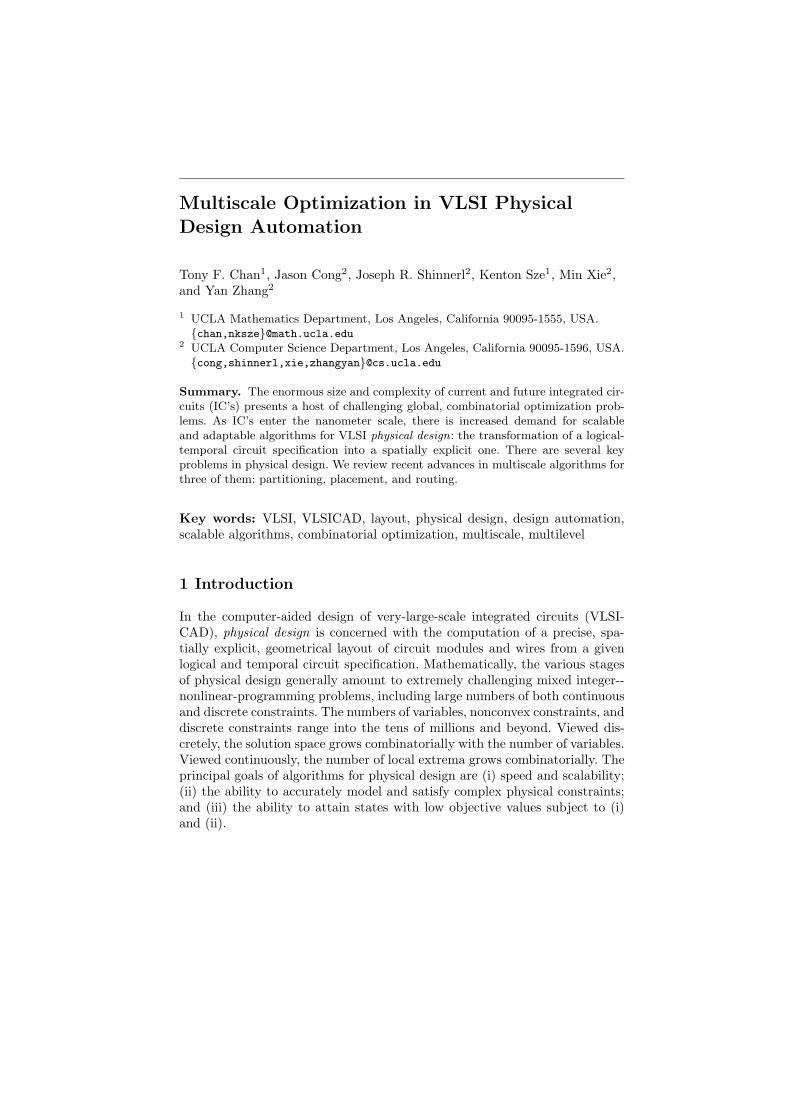
As illustrated in Figure 1, VLSI design can be divided into the followingsteps: system modeling, architectual synthesis, logic synthesis, physical design,fabrication, packaging.
• System modeling. The concepts in the designer’s mind are captured as a setof computational operations and data dependencies subject to constraintson timing, chip area, etc.
• Functional Design. The resources that can implement the system’s op-erations are identified, and the operations are scheduled. As a result, thecontrol logic and datapath interconnections are also identified. Functionaldesign is also called high-level synthesis.
• Logic synthesis. The high-level specification is transformed into an inter-connection of gate-level boolean primitives — nand, xor, etc. The circuitcomponents that can best realize the functions derived in functional de-sign are assembled. Circuit delay and power consumption are considered atthis step. The output description of the interconnection between differentgate-level primitives is usually called a netlist (Section 1.2).
• Physical design. The actual spatial layout of circuit components on thechip is determined. The objectives during this step usually include to-tal wirelength, maximum signal propogation time (“performance”), etc.Physical design can be further divided into steps including partitioning,floorplanning, placement, and routing; these are described in Section 1.2below.
• Fabrication. Fabrication involves the deposition and diffusion of materialonto a silicon wafer to achieve desired electronic circuit properties. Sincedesigns will make use of several layers of metal for wiring, masks mirroringthe layout on each metal layer will be applied in turn to produce therequired interconnection pattern by photolithography.
Multiscale Optimization in VLSI Physical Design Automation 5
System Modeling
Functional Design
Logic Synthesis
Fabrication
Packaging
Physical Design
Fig. 1. VLSI design includes system specification, functional design, logic design,physical design, fabrication, and packaging.
• Packaging. The wafer is diced into individual chips, which are then pack-aged and tested.
As the fundamental physical barriers to continued transistor miniaturiza-tion begin to take shape, efforts in synthesis and physical design have intensi-fied. The main component stages of physical design are reviewed next in moredetail.
1.2 Overview of VLSI Physical Design
At the physical level, an integrated circuit is a collection of rectangular mod-ules connected by rectangular wires. The wires are arranged in parallel, hori-zontal layers stacked along the z axis; the wires in each layer are also parallel.Each module has one face in a prescribed rectangle in the xy-plane known asthe placement region. However, different modules may intersect with differ-ent numbers of metal wiring layers. After logic synthesis, most modules are
6 Tony F. Chan et al.
Cell
multipin net
row
chip
Pin
two-pin net
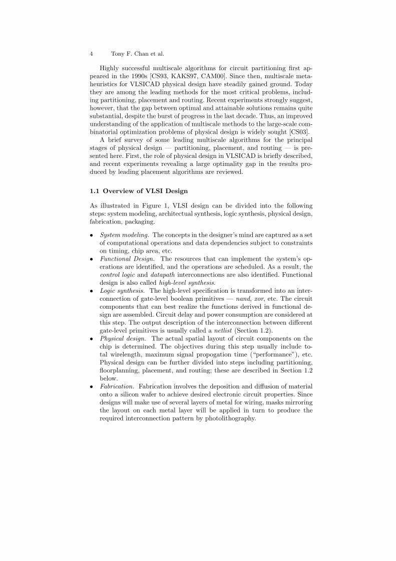
Fig. 2. A 2-D illustration of the physical elements of an integrated circuit. Therouting layers have been superimposed.
selected from a cell library and assigned to logic elements as part of a pro-cess known as technology mapping. These modules are called standard cells orsimply cells. Their widths (x-direction) may vary freely, but their heights (y-direction) are taken from a small, discrete set. Other, larger modules may rep-resent separately designed elements known as IP blocks (intellectual-propertyblocks) or macros; the heights of these larger blocks typically do not fall withinthe standard-cell heights or their integer multiples. The area of a module refersto the area of its cross-sections in the xy-plane.
A signal may propagate from a source point on a module to any number ofsinks on other modules. The source and sinks together define a net. At steadystate, a net is an equipotential of the circuit. A connection point between anet and a module is called a pin. Hence, a net may be abstracted as either aset of pins, or, less precisely, as the set of modules to which these pins belong.The netlist specifies the nets of a circuit as lists of pins and is a product oflogic synthesis (Section 1.1). The physical elements of an IC are illustrated inFigure 2.
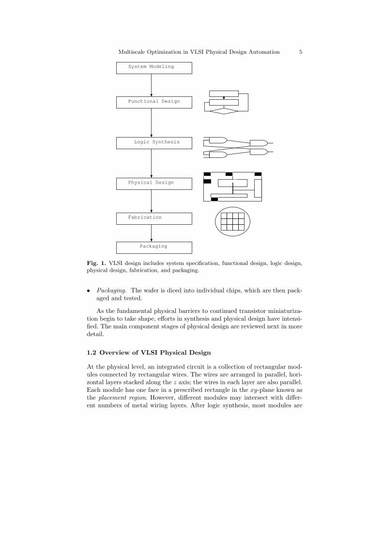
As illustrated in Figure 3, VLSI physical design proceeds through severalstages, including partitioning, floorplanning, placement, routing, and com-paction [DiM94, She99].
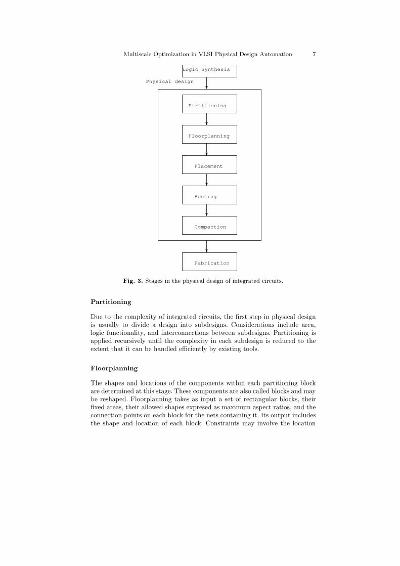
Multiscale Optimization in VLSI Physical Design Automation 7
Partitioning
Floorplanning
Placement
Routing
Compaction
Physical design
Fabrication
Logic Synthesis
Fig. 3. Stages in the physical design of integrated circuits.
Partitioning
Due to the complexity of integrated circuits, the first step in physical designis usually to divide a design into subdesigns. Considerations include area,logic functionality, and interconnections between subdesigns. Partitioning isapplied recursively until the complexity in each subdesign is reduced to theextent that it can be handled efficiently by existing tools.
Floorplanning
The shapes and locations of the components within each partitioning blockare determined at this stage. These components are also called blocks and maybe reshaped. Floorplanning takes as input a set of rectangular blocks, theirfixed areas, their allowed shapes expresed as maximum aspect ratios, and theconnection points on each block for the nets containing it. Its output includesthe shape and location of each block. Constraints may involve the location
8 Tony F. Chan et al.
of a block and/or adjacency requirements between arbitrary pairs of blocks.The blocks are not allowed to overlap. Floorplanning is typically limited toproblems with a few hundred or a few thousand blocks. As such, it is typicallyused as a means of coarse placement on a simplified circuit model, either as aprecursor to placement or as a means of guiding logic synthesis to a physicallyreasonable solution.
Placement
In contrast to floorplanning, placement treats the shapes of all blocks as fixed;i.e., it only determines the location of each block on the chip. The variablesare the xy-locations of the blocks; most blocks are standard cells (Section 1.2).The y-locations of cells are restricted to standard-cell rows, as in Figure 2.Placement instance sizes range into the tens of millions and will continue toincrease.
Placement is usually divided into two steps: global placement and detailedplacement. Global placement assigns blocks to certain subregions of the chipwithout determining the exact location of each component within its subre-gion. As a result, the blocks may still overlap. Detailed placement starts fromthe result of global placement, removes all overlap between blocks, and fur-ther optimizes the design. Placement objectives include the estimated totalwirelength needed to connect blocks in nets, the maximum expected wiringcongestion in subsequent routing, and/or the timing performance of the cir-cuit. A simplified formulation of placement is given in Section 1.5.1.
Routing
With the locations of the blocks fixed, their interconnections as specified bythe netlist must be realized. That is, the shapes and locations of the metalwires connecting the blocks must be determined. This wiring layout is per-formed not only within the placement region but also in a sequence of parallelmetal routing layers above it. Cells constitute routing obstacles in layers whichpass through them. Above the cells, all the wires in the same routing layer areparallel to the same coordinate axis, either x or y. Routing layers alternate inthe direction of their wires. Interlayer connections are called vias.
The objective of routing is to minimize the total wirelength while realizingall connections subject to wire spacing constraints within each layer. In addi-tion, the timing performance of the circuit may also be considered. Routing isusually done in two steps, global routing and detailed routing. Global-routingalgorithms determine a route for each connection in terms of the regions itpasses through, without giving the exact coordinates of the connection. Dur-ing this phase, the maximum congestion in each region must be kept below acertain limit. The goal of detailed routing is to realize a point-to-point pathfor each net following the guidance given by the global routing. It is in thisstep that the geometric location and shape of each wire is determined. Due
Multiscale Optimization in VLSI Physical Design Automation 9
to the sequential nature of most routing algorithms, a 100% completion ratemay not be obtained for many designs. An additional step called rip-up andreroute is used to remove a subset of connections already made and find alter-nate routes, so that the overall completion rate can be improved. The rip-upand reroute process works in an iterative fashion until either no improvementcan be obtained or a certain iteration limit is reached.
Compaction
Compaction is used to reduce the white space on the chip so that the chiparea can be minimized. This step involves heavy manipulation of geometricobjects. Depending on the movement these geometric objects are allowed,compaction can be categorized into 1-D compaction or 2-D compaction. How-ever, the chip area for many of the designs are given as fixed. In this case,instead of compacting the design, intelligent allocation of white space can beadopted to further optimize certain metrics, e.g., routing congestion, maxi-mum temperature, etc.
1.3 Hypergraph Circuit Model for Physical Design
An integrated circuit is abstracted more accurately as a hypergraph than asa graph, because each of its nets may connect not just a pair of nodes butrather an arbitrarily large subset of nodes. The details of the abstractiondepend on the point in the design flow where it is used. A generic definitionof the hypergraph concept is given here. In later sections, specific instances ofit are given for partitioning, placement, and routing.
A hypergraph H = {V, E} consists of a set of vertices V = {v1, v2, ...vn}and a set of hyperedges E = {e1, e2, . . . , em}. Each hyperedge ej is just somesubset of V , i.e., ej = {vj1 , vj1 , ...vjk} ⊂ V . Each hyperedge corresponds tosome net in the circuit. Each vertex vi may have weight w(vi) associated withit, e.g., area; each hyperedge ej may have weight w(ej) associated with it, e.g.,timing criticality. In either case, the hypergraph itself is said to be weighted aswell. The number of vertices contained by ej (we will also say “connected by”ej ) is called the degree of ej and is denoted |ej |. The number of hyperedgescontaining vi is called the degree of vi and is denoted |vi|.
Every hypergraph, weighted or unweighted, has a dual. The dual hyper-graph H ′ = {V ′, E′} of a given hypergraph H = {V, E} is defined as follows.First, let V ′ = E; if H is weighted, then let w(v′i) = w(ei). Second, for eachvi ∈ V , let e′i ∈ E′ be the set of ej ∈ E that contain vi. If H is weighted, thenlet w(e′i) = w(vi). It is straightforward to show that H ′′, the dual of H ′, isisomorphic to H.
1.4 The Gigascale Challenge
Since the early 1960s, the number of transistors in an integrated circuit hasdoubled roughly every 18 months. This trend, known as Moore’s Law, is ex-
10 Tony F. Chan et al.
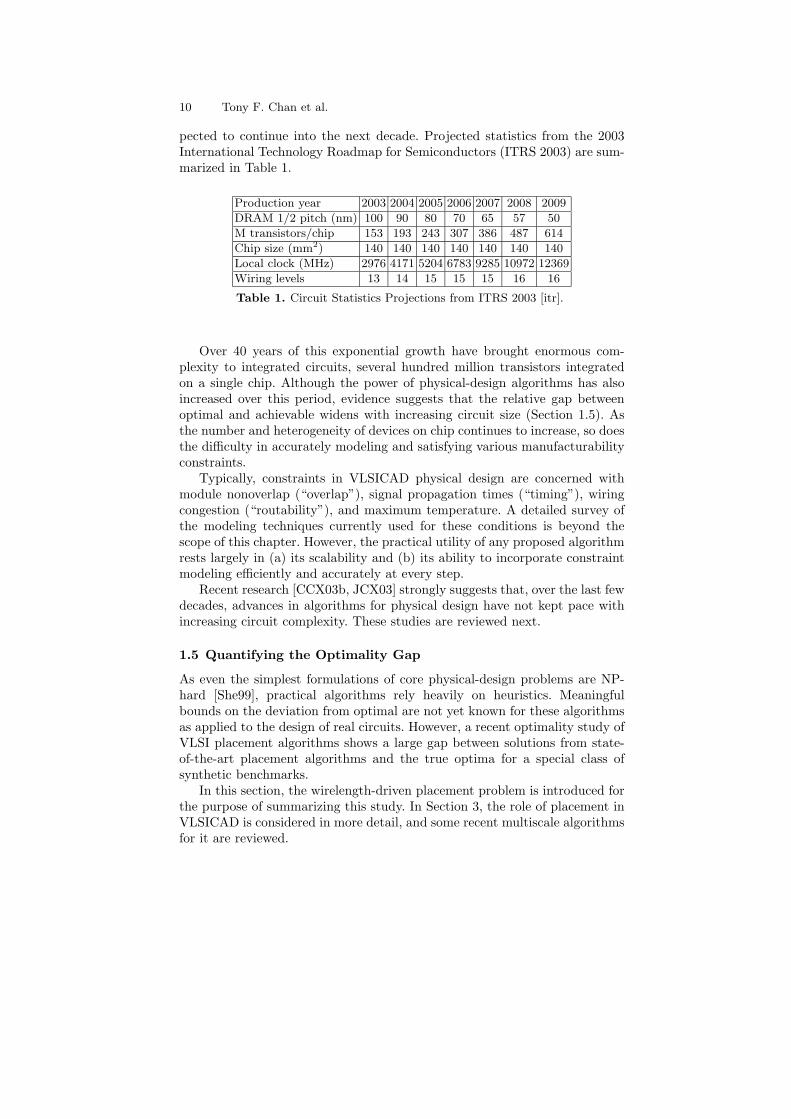
pected to continue into the next decade. Projected statistics from the 2003International Technology Roadmap for Semiconductors (ITRS 2003) are sum-marized in Table 1.
Production year 2003 2004 2005 2006 2007 2008 2009
DRAM 1/2 pitch (nm) 100 90 80 70 65 57 50
M transistors/chip 153 193 243 307 386 487 614
Chip size (mm2) 140 140 140 140 140 140 140
Local clock (MHz) 2976 4171 5204 6783 9285 10972 12369
Wiring levels 13 14 15 15 15 16 16
Table 1. Circuit Statistics Projections from ITRS 2003 [itr].
Over 40 years of this exponential growth have brought enormous com-plexity to integrated circuits, several hundred million transistors integratedon a single chip. Although the power of physical-design algorithms has alsoincreased over this period, evidence suggests that the relative gap betweenoptimal and achievable widens with increasing circuit size (Section 1.5). Asthe number and heterogeneity of devices on chip continues to increase, so doesthe difficulty in accurately modeling and satisfying various manufacturabilityconstraints.
Typically, constraints in VLSICAD physical design are concerned withmodule nonoverlap (“overlap”), signal propagation times (“timing”), wiringcongestion (“routability”), and maximum temperature. A detailed survey ofthe modeling techniques currently used for these conditions is beyond thescope of this chapter. However, the practical utility of any proposed algorithmrests largely in (a) its scalability and (b) its ability to incorporate constraintmodeling efficiently and accurately at every step.
Recent research [CCX03b, JCX03] strongly suggests that, over the last fewdecades, advances in algorithms for physical design have not kept pace withincreasing circuit complexity. These studies are reviewed next.
1.5 Quantifying the Optimality Gap
As even the simplest formulations of core physical-design problems are NP-hard [She99], practical algorithms rely heavily on heuristics. Meaningfulbounds on the deviation from optimal are not yet known for these algorithmsas applied to the design of real circuits. However, a recent optimality study ofVLSI placement algorithms shows a large gap between solutions from state-of-the-art placement algorithms and the true optima for a special class ofsynthetic benchmarks.
In this section, the wirelength-driven placement problem is introduced forthe purpose of summarizing this study. In Section 3, the role of placement inVLSICAD is considered in more detail, and some recent multiscale algorithmsfor it are reviewed.
Multiscale Optimization in VLSI Physical Design Automation 11
1.5.1 The Placement Model Problem
In the given hypergraph-netlist representation H = (V, E) of an integratedcircuit, we require for placement that each vi has a given, fixed rectangularshape. We assume given a bounded rectangle R in the plane whose boundariesare parallel to coordinate axes x and y. The orientation of each vi will also beassumed prescribed in alignment with the boundaries of R, although in somecases flipping vi across coordinate axes may be allowed. The length of vi alongthe x-axis is called its width; its length along the y-axis is called its height. Thevertices vi are typically represented at some fixed level of abstraction. Possiblelevels are, from lowest to highest, transistors, logic gates, standard cells, ormacros (cf. Section 1.2). As IC’s become more heterogeneous, the mixed-sizeproblem, in which elements from several of these levels are simultaneouslyplaced, increases in importance. The coverage in this chapter assumes theusual level of standard cells.
Interconnections among placed cells (Section 4) are ultimately made notonly within R but also in multiple routing layers above R; each routing layerhas the same x and y coordinates as R but a different z coordinate. For thisreason, the total area of all vi ∈ V may range anywhere from 50% to 98% ormore of the area of R. With multiple routing layers above placed cells, makingmetal connections between all the pins of a net can usually be accomplishedwithin the bounding box of the net. Therefore, the most commonly usedestimate of the length of wire `(ei) that will be required for routing a givennet ei = {vi1 , vi2 , . . . , vij} is simply the half-perimeter of its bounding box:
`(ei) =
(
maxk
x(vik)−minkx(vik)
)
+
(
maxk
y(vik)−minky(vik)
)
. (1)
Wirelength-Driven Model Problem
In the simplest commonly used abstraction of placement, total 2D-bounding-box wirelength is minimized subject to the pairwise nonoverlap, row-alignment,and placement-boundary constraints. Let w(R) denote the width (along thex-direction) of the placement region R, and let Y1, Y2, . . . , Ynr denote the y-coordinates of its standard-cell rows’ centers; assume every cell fits in everyrow. With (xi, yi) denoting the center of cell vi and wi denoting its width,this wirelength-driven form of placement may be expressed as
min(xi, yi)
∑
e∈E w(e)`(e) for `(e) defined in (1)
subject to yi ∈ {Y1, . . . , Ynr} all vi ∈ V0 ≤ xi ≤ w(R)− wi/2 all vi ∈ V|xi − xj | > (wi + wj)/2 or yi 6= yj all vi, vj ∈ V.
(2)
Despite its apparent simplicity, this formulation captures much of the difficultyin placement. High-quality solutions to (2) generally serve as useful starting
12 Tony F. Chan et al.
F
G J
D H
A B
E
C
I
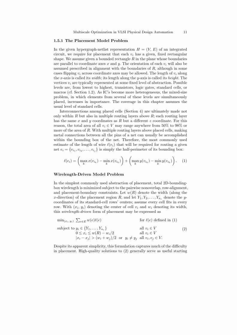
Fig. 4. PEKO generation for p = 9, D = (6,2,2).
points for more elaborate models of real circuits. The optimality gap for mostleading academic tools applied to (2) has been observed to be quite large forthe PEKO benchmarks discussed next.
1.5.2 Placement Examples with Known Optima (PEKO)
Placement algorithms have been actively studied for the past 30 years. How-ever, there is little understanding of how far computed solutions are fromoptimal. It is also not known how much the deviation from optimality islikely to grow with respect to problem size. Recently, significant progress wasmade toward answers to these questions using cleverly constructed placementexamples with known optima (PEKO) [CCX03a].
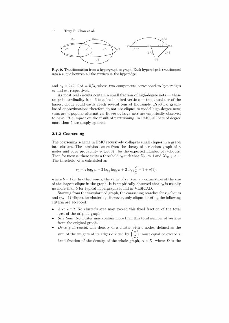
The construction of PEKO can be stated as follows. Given a netlist N , letD(N) = (d2, d3, . . . , dn) be the Net Distribution Vector (NDV ), where dk isthe total number of k-pin nets in the netlist. PEKO examples have all cellsof equal size. Given a number p and a vector D, we construct a placementexample with p placeable cells such that (i) its netlist has D as its NDV and(ii) it has a known placement of optimal half-perimeter wirelength. The cellsare first arranged in a nearly square rectangular region as a regular 2-D arrayof uniform rows and columns, except possibly the last row, which may not befilled. After that, nets are defined one by one on the cells in such a way thatthe bounding box for each net has minimal perimeter. Each k-pin net connects
cells within a region of size⌈√
k⌉
×⌈
k/⌈√
k⌉⌉
(or⌈
k/⌈√
k⌉⌉
×⌈√
k⌉
). The
wirelength for each k-pin net thus constructed is optimal. In the end, thespecific netlist is extracted from this placed configuration.
Figure 4 shows an example, where p = 9, D = (6, 2, 2). Net A is a 4-pinnet. Accordingly, it will connect four cells located in a 2×2 rectangular region.In Figure 4, it connects the four cells in the lower left corner. The other 4-pinnet, B, is placed on the lower right corner. Using the same method, the two 3-pin nets are generated as C and D respectively. This process is repeated untilthe NDV is exhausted. The total wirelength for this example is 6*1+2*2+2*2
Multiscale Optimization in VLSI Physical Design Automation 13
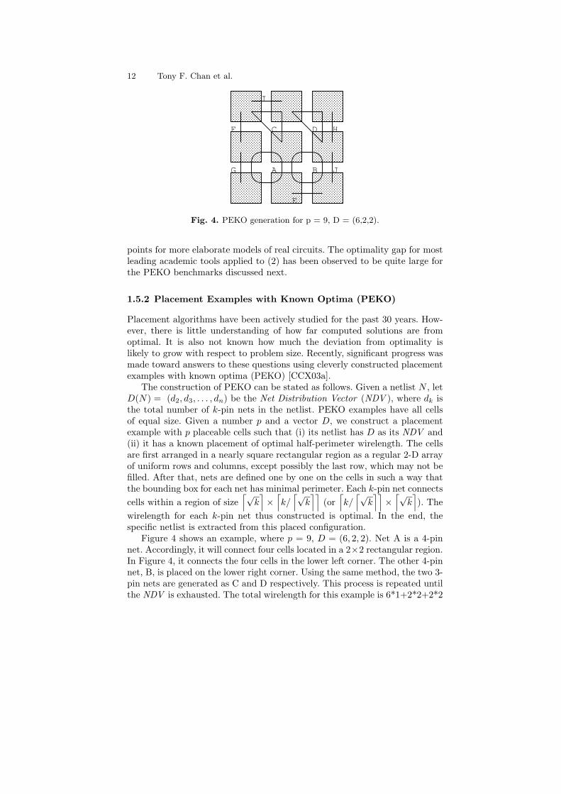
Fig. 5. An 8×8 PEKO instance.
= 14. To mimic real circuits, the NDV used in [CCX03a] to generate PEKOare extracted from real circuits [Alp98].
Another, still tiny example with a more realistic NDV is shown in Figure 5.Four state-of-the-art placers from academia including Dragon [WYS00a],
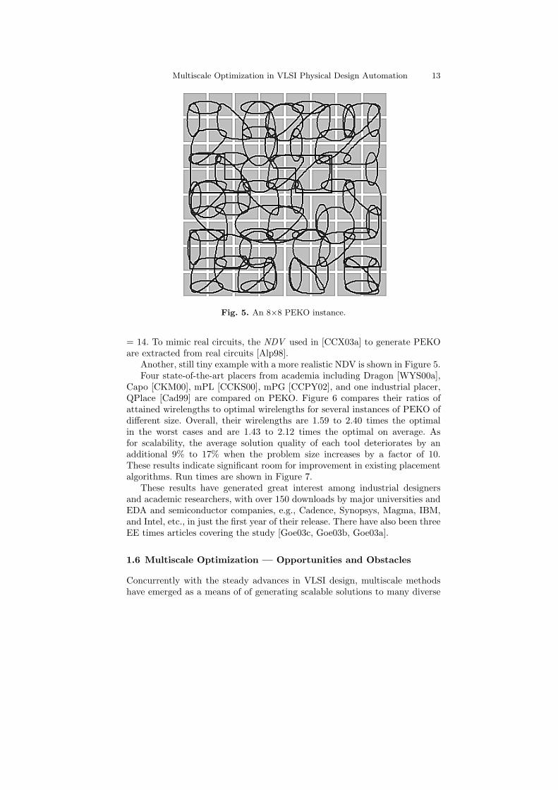
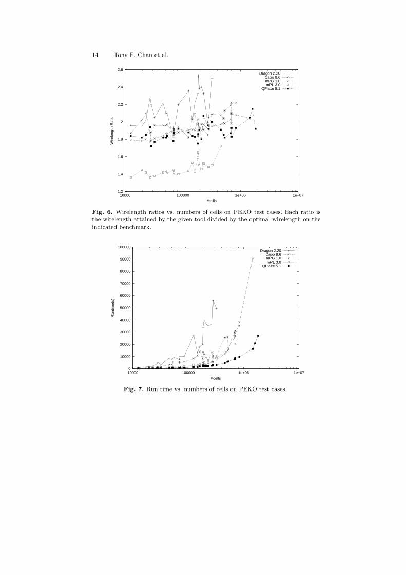
Capo [CKM00], mPL [CCKS00], mPG [CCPY02], and one industrial placer,QPlace [Cad99] are compared on PEKO. Figure 6 compares their ratios ofattained wirelengths to optimal wirelengths for several instances of PEKO ofdifferent size. Overall, their wirelengths are 1.59 to 2.40 times the optimalin the worst cases and are 1.43 to 2.12 times the optimal on average. Asfor scalability, the average solution quality of each tool deteriorates by anadditional 9% to 17% when the problem size increases by a factor of 10.These results indicate significant room for improvement in existing placementalgorithms. Run times are shown in Figure 7.
These results have generated great interest among industrial designersand academic researchers, with over 150 downloads by major universities andEDA and semiconductor companies, e.g., Cadence, Synopsys, Magma, IBM,and Intel, etc., in just the first year of their release. There have also been threeEE times articles covering the study [Goe03c, Goe03b, Goe03a].
1.6 Multiscale Optimization — Opportunities and Obstacles
Concurrently with the steady advances in VLSI design, multiscale methodshave emerged as a means of of generating scalable solutions to many diverse
14 Tony F. Chan et al.
1.2
1.4
1.6
1.8
2
2.2
2.4
2.6
10000 100000 1e+06 1e+07
Wire
leng
th R
atio
#cells
Dragon 2.20Capo 8.6mPG 1.0mPL 3.0
QPlace 5.1
Fig. 6. Wirelength ratios vs. numbers of cells on PEKO test cases. Each ratio isthe wirelength attained by the given tool divided by the optimal wirelength on theindicated benchmark.
0
10000
20000
30000
40000
50000
60000
70000
80000
90000
100000
10000 100000 1e+06 1e+07
Run
time(
s)
#cells
Dragon 2.20Capo 8.6mPG 1.0mPL 3.0
QPlace 5.1
Fig. 7. Run time vs. numbers of cells on PEKO test cases.
Multiscale Optimization in VLSI Physical Design Automation 15
mathematical problems in the gigascale range. However, multiscale methodsfor PDEs are not readily transferred to the large-scale combinatorial opti-mization problems common to VLSICAD. A lack of continuity presents oneobstacle. The presence of myriad local extrema presents another. Nevertheless,in recent years, multiscale methods have also been successfully applied to VL-SICAD [CS03]. In circuit partitioning, hMetis and MLpart [KAKS97, CAM00]produce the best cutsize minimization, and MLPR [CW02] produces the bestbalance of timing delay and cutsize. Significant progress has also been madein multiscale placement [SR99, CCK+03, SWY02, CCPY02, KW04, HMS04]and routing [CFZ01, CXZ02, CL04].
Hierarchical levels of abstraction are indispensable in the design of gi-gascale complex systems, but hierarchies must properly represent physicalrelationships, viz., interconnects, among constituent parts. The flexibility ofthe multiscale heuristic provides the opportunity both to merge previouslydistinct phases in the design flow and to simultaneously model very diverse,heterogeneous kinds of constraints.
1.7 An Operative Definition of Multiscale Optimization
The engineering complexity of VLSICAD has led researchers to a large varietyof algorithms and terminology quite distinct from what exists in other areas.In this section, we take a fairly inclusive view and try not to impose artificialdistinctions. By multiscale optimization, we mean
(i) the use of optimization at every level of a hierarchy of problem formula-tions, wherein
(ii) each variable at any given coarser level represents a subset of variables atthe adjacent finer level.
In particular, each coarse-level formulation can be viewed directly as a coarserepresentation of the original problem. Therefore, coarse-level solutions im-plicitly provide approximate solutions at the finest level as well. While manylong-standing paradigms in VLSICAD employ optimization hierarchically,multiscale algorithms as defined above are a relatively new phenomenon. Thisdistinction is considered further in Section 3.2.
The terms multilevel and multiscale are used synonomously.
Characterization of Multiscale Algorithms
1. Hierarchy Construction. Although the construction is usually from thebottom up by recursive aggregation, top-down constructions are also pos-sible, as described in Section 3.4 below.
2. Relaxation. In the combinatorial setting, the purpose of intralevel opti-mization is not generally viewed as error smoothing but rather the effi-cient, iterative exploration of the solution space at that level. Continuous,discrete, local, global, stochastic, and deterministic formulations may beused in various combinations.
16 Tony F. Chan et al.
3. Interpolation. A coarse-level solution can be transferred to and repre-sented at its adjacent finer level in a variety of ways. The simplest andmost common is simply the placement of all components of a cluster con-centrically at the cluster’s center. This choice amounts to a piecewise-constant interpolation.
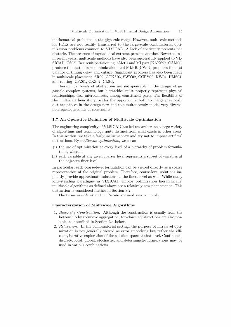
4. Iteration Flow. The levels of the hierarchy may be traversed in differentways. A single pass from the coarsest to the finest level is still the mostcommon. Alternatives include standard flows such as a single V-cycle,multiple V-cycles, W-cycles, and the full multigrid (FMG) F-cycle (seeFigure 8 on Page 16).
The forms taken by these components are usually tightly coupled with thediverse objective models and constraint models used by different algorithms.
Fig. 8. Some iteration flows for multiscale optimization.
2 Multiscale Hypergraph Partitioning
Given a hypergraph H = {V, E}, the hypergraph partitioning problem is topartition V into disjoint subsets P = {V1, V2, ..., Vk}, i.e.,
Vi ∩ Vj = φ for i 6= j, and ∪ Vi = V,
subject to certain objectives and constraints. Each block Vi of partition P isalso called a partition. The area of partition Vi is defined as
area(Vi) =∑
v∈Viarea(v)
Multiscale Optimization in VLSI Physical Design Automation 17
The objective in hypergraph partitioning is usually to minimize the cutsize,the number of hyperedges that connect vertices from two different partitionblocks.
Typical constraints in the hypergraph partitioning problem include thefollowing.
• The relative area of each partition block. E.g., li × area(V ) ≤ area(Vi) ≤ui × area(V ) for user-specified parameters li and ui.
• The number of partition blocks k. When k = 2, the problem is calledbipartitioning. When k > 2, the problem is called multiway partitioning.Multiway partitioning problems are often reduced to a recursive sequenceof bipartitioning problems.
We focus on bipartitioning algorithms for the rest of this section.
2.1 Early Multiscale Hypergraph Partitioning: FMC
An early effort to accelerate the standard Fiduccia-Mattheyses Algorithm(FM, Figure 10 on Page 19) by recursive clustering was made without anydeliberate connection to existing multiscale algorithms [CS93]. To facilitatecoarsening, a graph corresponding to the original hypergraph is constructed. Abottom-up clustering algorithm is applied to recursively collapse small cliquesinto clusters. An iterative-refinement algorithm is then applied to the clusteredhypergraph to optimize the cutsize, satisfying the area constraint at the sametime. This refinement is coupled with a recursive declustering process untilthe partitioning result on the original hypergraph is obtained. This early workis referred to as FMC (FM with clustering).
2.1.1 Hypergraph-to-graph transformation
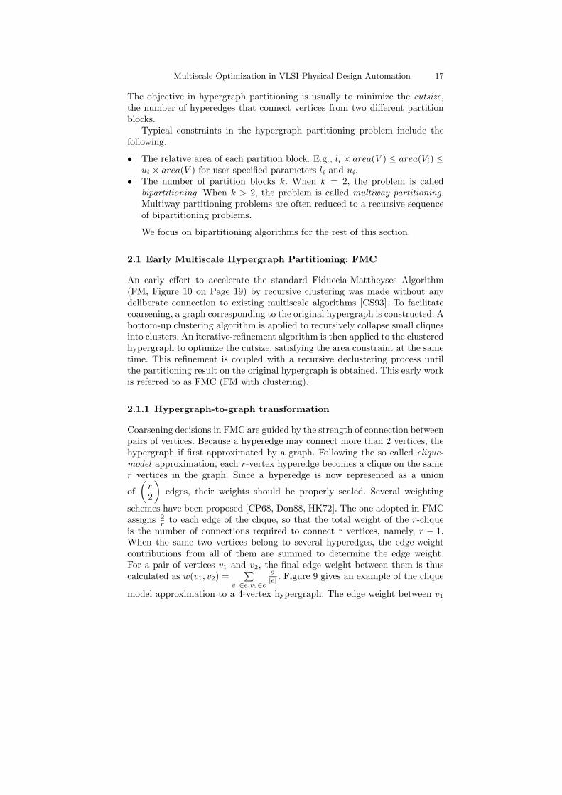
Coarsening decisions in FMC are guided by the strength of connection betweenpairs of vertices. Because a hyperedge may connect more than 2 vertices, thehypergraph if first approximated by a graph. Following the so called clique-model approximation, each r-vertex hyperedge becomes a clique on the samer vertices in the graph. Since a hyperedge is now represented as a union
of
(r2
)
edges, their weights should be properly scaled. Several weighting
schemes have been proposed [CP68, Don88, HK72]. The one adopted in FMCassigns 2
r to each edge of the clique, so that the total weight of the r-cliqueis the number of connections required to connect r vertices, namely, r − 1.When the same two vertices belong to several hyperedges, the edge-weightcontributions from all of them are summed to determine the edge weight.For a pair of vertices v1 and v2, the final edge weight between them is thuscalculated as w(v1, v2) =
∑
v1∈e,v2∈e2|e| . Figure 9 gives an example of the clique
model approximation to a 4-vertex hypergraph. The edge weight between v1
18 Tony F. Chan et al.
v1v2 v3
v4
v2 v3v1
v4
e1 e2
2/3 2/3
2/3
4/35/3e3
Fig. 9. Transformation from a hypergraph to graph. Each hyperedge is transformedinto a clique between all the vertices in the hyperedge.
and v2 is 2/2+2/3 = 5/3, whose two components correspond to hyperedgese1 and e3, respectively.
As most real circuits contain a small fraction of high-degree nets — theserange in cardinality from 6 to a few hundred vertices — the actual size of thelargest clique could easily reach several tens of thousands. Practical graph-based approximations therefore do not use cliques to model high-degree nets;stars are a popular alternative. However, large nets are empirically observedto have little impact on the result of partitioning. In FMC, all nets of degreemore than 5 are simply ignored.
2.1.2 Coarsening
The coarsening scheme in FMC recursively collapses small cliques in a graphinto clusters. The intuition comes from the theory of a random graph of nnodes and edge probability p. Let Xr be the expected number of r-cliques.Then for most n, there exists a threshold r0 such thatXr0 � 1 andXr0+1 < 1.The threshold r0 is calculated as
r0 = 2 logb n− 2 logb logb n+ 2 logbe
2+ 1 + o(1),
where b = 1/p. In other words, the value of r0 is an approximation of the sizeof the largest clique in the graph. It is empirically observed that r0 is usuallyno more than 5 for typical hypergraphs found in VLSICAD.
Starting from the transformed graph, the coarsening searches for r0-cliquesand (r0+1)-cliques for clustering. However, only cliques meeting the followingcriteria are accepted.
• Area limit. No cluster’s area may exceed this fixed fraction of the totalarea of the original graph.
• Size limit. No cluster may contain more than this total number of verticesfrom the original graph.
• Density threshold. The density of a cluster with c nodes, defined as the
sum of the weights of its edges divided by
(c2
)
, must equal or exceed a
fixed fraction of the density of the whole graph, α × D, where D is the
Multiscale Optimization in VLSI Physical Design Automation 19
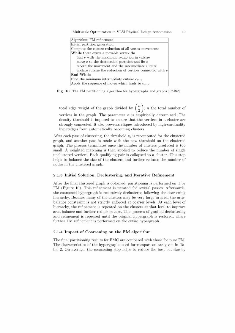
Algorithm: FM refinement
Initial partition generationCompute the cutsize reduction of all vertex movementsWhile there exists a movable vertex do
find v with the maximum reduction in cutsizemove v to the destination partition and fix vrecord the movement and the intermediate cutsizeupdate cutsize the reduction of vertices connected with v
End While
Find the minimum intermediate cutsize cminApply the sequence of moves which leads to cmin
Fig. 10. The FM partitioning algorithm for hypergraphs and graphs [FM82].
total edge weight of the graph divided by
(n2
)
, n the total number of
vertices in the graph. The parameter α is empirically determined. Thedensity threshold is imposed to ensure that the vertices in a cluster arestrongly connected. It also prevents cliques introduced by high-cardinalityhyperedges from automatically becoming clusters.
After each pass of clustering, the threshold r0 is recomputed for the clusteredgraph, and another pass is made with the new threshold on the clusteredgraph. The process terminates once the number of clusters produced is toosmall. A weighted matching is then applied to reduce the number of singleunclustered vertices. Each qualifying pair is collapsed to a cluster. This stephelps to balance the size of the clusters and further reduces the number ofnodes in the clustered graph.
2.1.3 Initial Solution, Declustering, and Iterative Refinement
After the final clustered graph is obtained, partitioning is performed on it byFM (Figure 10). This refinement is iterated for several passes. Afterwards,the coarsened hypergraph is recursively declustered following the coarseninghierarchy. Because many of the clusters may be very large in area, the area-balance constraint is not strictly enforced at coarser levels. At each level ofhierarchy, the refinement is repeated on the clusters at that level to improvearea balance and further reduce cutsize. This process of gradual declusteringand refinement is repeated until the original hypergraph is restored, wherefurther FM refinement is performed on the entire hypergraph.
2.1.4 Impact of Coarsening on the FM algorithm
The final partitioning results for FMC are compared with those for pure FM.The characteristics of the hypergraphs used for comparison are given in Ta-ble 2. On average, the coarsening step helps to reduce the best cut size by

20 Tony F. Chan et al.
hypergraph #vertices #hyperedgesBest Cut Avg. CutFM FMC FM FMC
8870 502 494 17 15 27.4 17.3
bm1 882 902 65 53 82.9 69.6
PrimGA1 733 902 48 49 69.2 64.7
PrimSC1 733 902 46 45 74 56.2
5655 921 760 54 48 67.9 62.6
Test04 1515 1658 44 44 46 48.4
Test03 1607 1618 93 64 137.9 80.1
Test02 1663 1721 121 80 181.1 105.9
Test06 1752 1674 60 64 79.9 74.8
Test05 2595 2751 42 42 61.3 57.5
19ks 2844 3282 151 129 173.7 156.1
PrimGA2 3014 3029 246 130 284 181.3
PrimSC2 3014 3029 199 130 277.2 229.1
industry2 12142 12949 458 315 812.6 402.3
Avg. 16.60% 21.20%
Table 2. Impact of coarsening on FM algorithm. On average, coarsening helps toreduce the best cut size by 16.6%. It reduces the average cut size by 21.2% [CS93].
16.6%. It reduces the average cut size by 21.2%. The impact of coarsening onthe refinement stage is obvious in this scenario. The results are very promis-ing; however, they do not demonstrate the full power of multiscale methods.There are several limitations in this work. First, the coarsening scheme onlycollapses cliques. This artificially imposed constraint will eliminate many pos-sible coarsening candidates which might lead to better final cutsize. Second,its control on the cluster size is limited. Since a whole clique is collapsed eachtime, the coarsened graph tends to become more uneven in cluster size.
To our knowledge, FMC is the first application of multiscale optimizationto circuit partitioning. Following FMC, there have been several efforts toapply multiscale methods to the hypergraph partitioning problem [AHK97,KAKS97, CLW99, CL00, CLW00, CAM00]. Among the most successful arehMetis [KAKS97] and MLpart [CAM00], described next.
2.2 hMetis
hMetis [KAKS97, Kar99, Kar02] was first proposed for bipartitioning andlater extended to multiway partitioning. Its iteration flow is a sequence of thetraditional multiscale V-cycles shown in Figure 11. It constructs a hierarchyof partitioning problems by recursive clustering, generates multiple initial-solution candidates, then recursively declusters and refines at each level. Itimproves its candidate solutions at each level of declustering by FM-basedlocal relaxation (Figure 10). A certain fraction of the poorest solution can-didates is discarded after relaxation so as not to incur excessive run-time at
Multiscale Optimization in VLSI Physical Design Automation 21
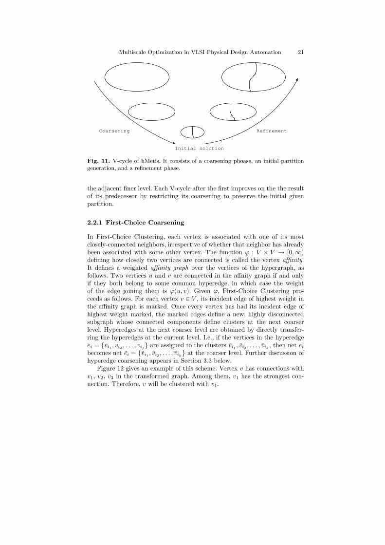
Coarsening Refinement
Initial solution
Fig. 11. V-cycle of hMetis. It consists of a coarsening phoase, an initial partitiongeneration, and a refinement phase.
the adjacent finer level. Each V-cycle after the first improves on the the resultof its predecessor by restricting its coarsening to preserve the initial givenpartition.
2.2.1 First-Choice Coarsening
In First-Choice Clustering, each vertex is associated with one of its mostclosely-connected neighbors, irrespective of whether that neighbor has alreadybeen associated with some other vertex. The function ϕ : V × V → [0,∞)defining how closely two vertices are connected is called the vertex affinity.It defines a weighted affinity graph over the vertices of the hypergraph, asfollows. Two vertices u and v are connected in the affnity graph if and onlyif they both belong to some common hyperedge, in which case the weightof the edge joining them is ϕ(u, v). Given ϕ, First-Choice Clustering pro-ceeds as follows. For each vertex v ∈ V , its incident edge of highest weight inthe affinity graph is marked. Once every vertex has had its incident edge ofhighest weight marked, the marked edges define a new, highly disconnectedsubgraph whose connected components define clusters at the next coarserlevel. Hyperedges at the next coarser level are obtained by directly transfer-ring the hyperedges at the current level. I.e., if the vertices in the hyperedgeei = {vi1 , vi2 , . . . , vij} are assigned to the clusters vi1 , vi2 , . . . , vik , then net eibecomes net ei = {vi1 , vi2 , . . . , vik} at the coarser level. Further discussion ofhyperedge coarsening appears in Section 3.3 below.
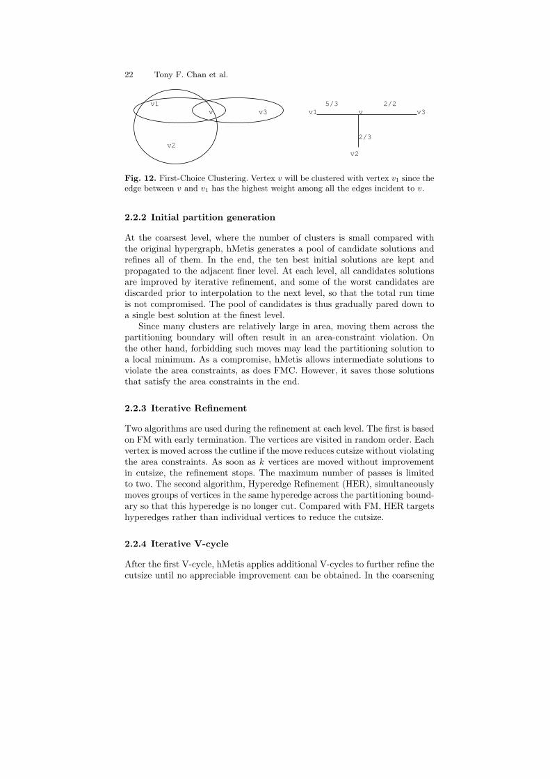
Figure 12 gives an example of this scheme. Vertex v has connections withv1, v2, v3 in the transformed graph. Among them, v1 has the strongest con-nection. Therefore, v will be clustered with v1.
22 Tony F. Chan et al.
v1
v2
v3v v v3v1
v2
2/25/3
2/3
Fig. 12. First-Choice Clustering. Vertex v will be clustered with vertex v1 since theedge between v and v1 has the highest weight among all the edges incident to v.
2.2.2 Initial partition generation
At the coarsest level, where the number of clusters is small compared withthe original hypergraph, hMetis generates a pool of candidate solutions andrefines all of them. In the end, the ten best initial solutions are kept andpropagated to the adjacent finer level. At each level, all candidates solutionsare improved by iterative refinement, and some of the worst candidates arediscarded prior to interpolation to the next level, so that the total run timeis not compromised. The pool of candidates is thus gradually pared down toa single best solution at the finest level.
Since many clusters are relatively large in area, moving them across thepartitioning boundary will often result in an area-constraint violation. Onthe other hand, forbidding such moves may lead the partitioning solution toa local minimum. As a compromise, hMetis allows intermediate solutions toviolate the area constraints, as does FMC. However, it saves those solutionsthat satisfy the area constraints in the end.
2.2.3 Iterative Refinement
Two algorithms are used during the refinement at each level. The first is basedon FM with early termination. The vertices are visited in random order. Eachvertex is moved across the cutline if the move reduces cutsize without violatingthe area constraints. As soon as k vertices are moved without improvementin cutsize, the refinement stops. The maximum number of passes is limitedto two. The second algorithm, Hyperedge Refinement (HER), simultaneouslymoves groups of vertices in the same hyperedge across the partitioning bound-ary so that this hyperedge is no longer cut. Compared with FM, HER targetshyperedges rather than individual vertices to reduce the cutsize.
2.2.4 Iterative V-cycle
After the first V-cycle, hMetis applies additional V-cycles to further refine thecutsize until no appreciable improvement can be obtained. In the coarsening
Multiscale Optimization in VLSI Physical Design Automation 23
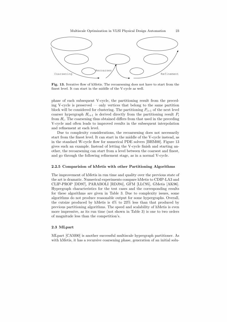
CoarseningRecoarsen
Refinement
Fig. 13. Iterative flow of hMetis. The recoarsening does not have to start from thefinest level. It can start in the middle of the V-cycle as well.
phase of each subsequent V-cycle, the partitioning result from the preced-ing V-cycle is preserved — only vertices that belong to the same partitionblock will be considered for clustering. The partitioning Pi+1 of the next levelcoarser hypergraph Hi+1 is derived directly from the partitioning result Pifrom Hi. The coarsening thus obtained differs from that used in the precedingV-cycle and often leads to improved results in the subsequent interpolationand refinement at each level.
Due to complexity considerations, the recoarsening does not necessarilystart from the finest level. It can start in the middle of the V-cycle instead, asin the standard W-cycle flow for numerical PDE solvers [BHM00]. Figure 13gives such an example. Instead of letting the V-cycle finish and starting an-other, the recoarsening can start from a level between the coarsest and finest,and go through the following refinement stage, as in a normal V-cycle.
2.2.5 Comparision of hMetis with other Partitioning Algorithms
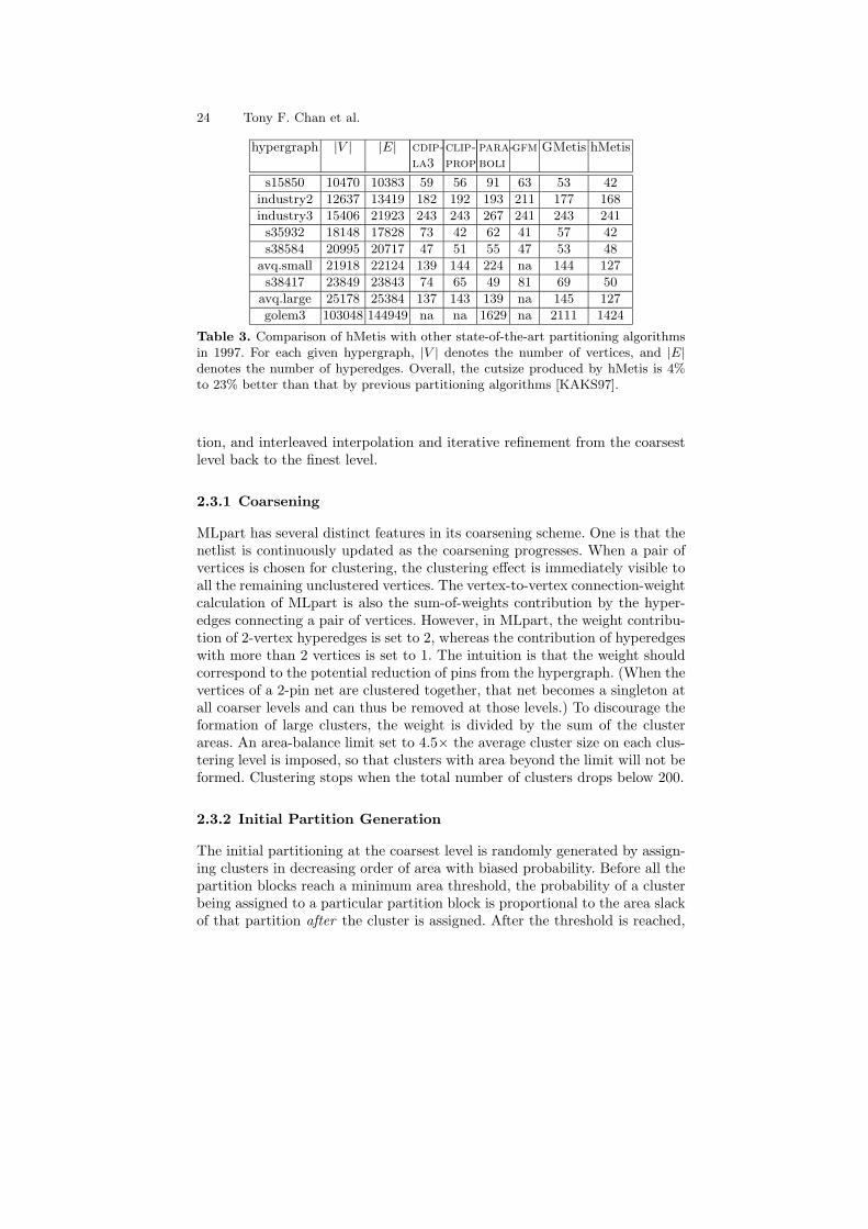
The improvement of hMetis in run time and quality over the previous state ofthe art is dramatic. Numerical experiments compare hMetis to CDIP-LA3 andCLIP-PROP [DD97], PARABOLI [RDJ94], GFM [LLC95], GMetis [AK96].Hypergraph characteristics for the test cases and the corresponding resultsfor these algorithms are given in Table 3. Due to complexity issues, somealgorithms do not produce reasonable output for some hypergraphs. Overall,the cutsize produced by hMetis is 4% to 23% less than that produced byprevious partitioning algorithms. The speed and scalability of hMetis is evenmore impressive, as its run time (not shown in Table 3) is one to two ordersof magnitude less than the competition’s.
2.3 MLpart
MLpart [CAM00] is another successful multiscale hypergraph partitioner. Aswith hMetis, it has a recursive coarsening phase, generation of an initial solu-
24 Tony F. Chan et al.
hypergraph |V | |E| cdip-la3
clip-prop
para-boli
gfm GMetis hMetis
s15850 10470 10383 59 56 91 63 53 42
industry2 12637 13419 182 192 193 211 177 168
industry3 15406 21923 243 243 267 241 243 241
s35932 18148 17828 73 42 62 41 57 42
s38584 20995 20717 47 51 55 47 53 48
avq.small 21918 22124 139 144 224 na 144 127
s38417 23849 23843 74 65 49 81 69 50
avq.large 25178 25384 137 143 139 na 145 127
golem3 103048 144949 na na 1629 na 2111 1424
Table 3. Comparison of hMetis with other state-of-the-art partitioning algorithmsin 1997. For each given hypergraph, |V | denotes the number of vertices, and |E|denotes the number of hyperedges. Overall, the cutsize produced by hMetis is 4%to 23% better than that by previous partitioning algorithms [KAKS97].
tion, and interleaved interpolation and iterative refinement from the coarsestlevel back to the finest level.
2.3.1 Coarsening
MLpart has several distinct features in its coarsening scheme. One is that thenetlist is continuously updated as the coarsening progresses. When a pair ofvertices is chosen for clustering, the clustering effect is immediately visible toall the remaining unclustered vertices. The vertex-to-vertex connection-weightcalculation of MLpart is also the sum-of-weights contribution by the hyper-edges connecting a pair of vertices. However, in MLpart, the weight contribu-tion of 2-vertex hyperedges is set to 2, whereas the contribution of hyperedgeswith more than 2 vertices is set to 1. The intuition is that the weight shouldcorrespond to the potential reduction of pins from the hypergraph. (When thevertices of a 2-pin net are clustered together, that net becomes a singleton atall coarser levels and can thus be removed at those levels.) To discourage theformation of large clusters, the weight is divided by the sum of the clusterareas. An area-balance limit set to 4.5× the average cluster size on each clus-tering level is imposed, so that clusters with area beyond the limit will not beformed. Clustering stops when the total number of clusters drops below 200.
2.3.2 Initial Partition Generation
The initial partitioning at the coarsest level is randomly generated by assign-ing clusters in decreasing order of area with biased probability. Before all thepartition blocks reach a minimum area threshold, the probability of a clusterbeing assigned to a particular partition block is proportional to the area slackof that partition after the cluster is assigned. After the threshold is reached,
Multiscale Optimization in VLSI Physical Design Automation 25
the probability is proportional to the maximum allowed area of each cluster.Following the random initial generation, FM-based refinement is applied tothe initial solution. Similar to hMetis, multiple initial solutions are generated,but only the best solution is kept and propagated to finer levels.
2.3.3 Iterative refinement
The refinement of MLpart is also based on FM. The authors also note thatstrictly satisfying the area constraint at coarser levels does not lead to thesmallest possible cutsize at the finest level. Therefore, the acceptance criteriaof a cluster movement is relaxed so that a move is accepted as long as it doesnot increase the violation of balance constraints. It is empirically observedthat, although the area-balance criterion is relaxed, the refinement can usuallyreach a legal solution with smaller cutsize after the first pass.
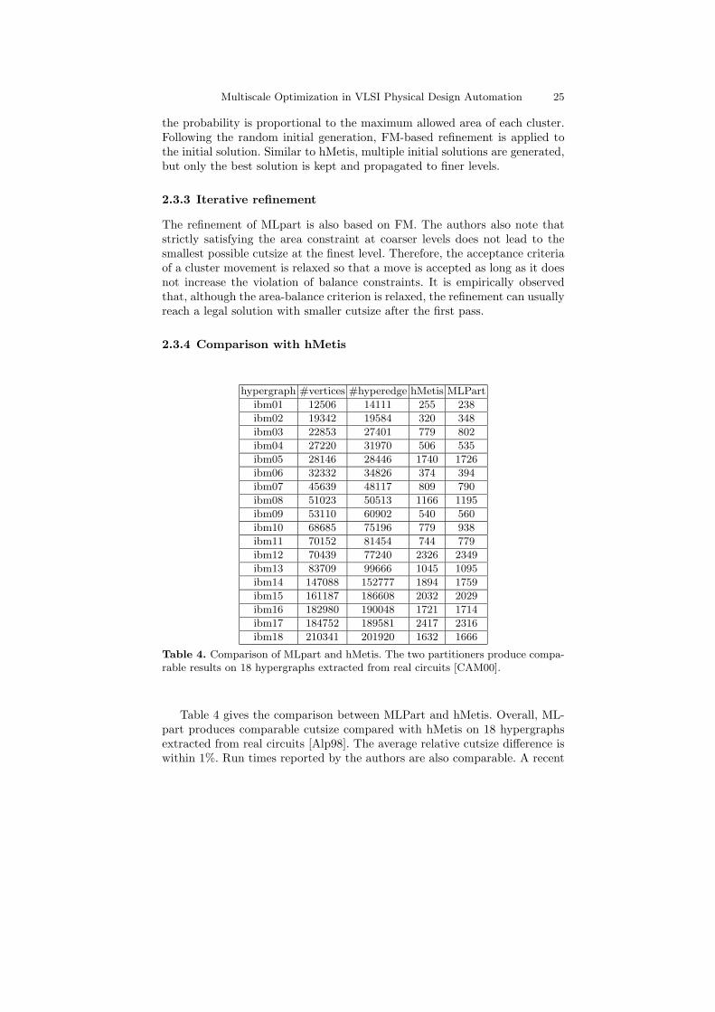
2.3.4 Comparison with hMetis
hypergraph #vertices #hyperedge hMetis MLPart
ibm01 12506 14111 255 238
ibm02 19342 19584 320 348
ibm03 22853 27401 779 802
ibm04 27220 31970 506 535
ibm05 28146 28446 1740 1726
ibm06 32332 34826 374 394
ibm07 45639 48117 809 790
ibm08 51023 50513 1166 1195
ibm09 53110 60902 540 560
ibm10 68685 75196 779 938
ibm11 70152 81454 744 779
ibm12 70439 77240 2326 2349
ibm13 83709 99666 1045 1095
ibm14 147088 152777 1894 1759
ibm15 161187 186608 2032 2029
ibm16 182980 190048 1721 1714
ibm17 184752 189581 2417 2316
ibm18 210341 201920 1632 1666
Table 4. Comparison of MLpart and hMetis. The two partitioners produce compa-rable results on 18 hypergraphs extracted from real circuits [CAM00].
Table 4 gives the comparison between MLPart and hMetis. Overall, ML-part produces comparable cutsize compared with hMetis on 18 hypergraphsextracted from real circuits [Alp98]. The average relative cutsize difference iswithin 1%. Run times reported by the authors are also comparable. A recent
26 Tony F. Chan et al.
optimality study of partitioning algorithms, however, suggests that MLpartmay be considerably more robust than hMetis. On a certain class of syntheticbipartitioning benchmarks with known upper bounds on optimal cutsize, ML-part consistently obtains cuts attaining the upper bounds, while hMetis findscuts up to 20% worse [JCX03, CCRX04].
3 Multiscale Placement
The spatial arrangement of circuit elements fundamentally constrains the lay-out of the circuit’s interconnect and, therefore, the signal timing of the inte-grated circuit. Thus, as interconnect delay continues to increase relative to de-vice delay, the importance of a good placement also increases. Rapid progressin placement has been made in the last few years independently across sev-eral different families of algorithms, with order-of-magnitude improvements inrun-time and quality. Significant challenges remain, however, particularly withrespect to the increasing size, complexity, and heterogeneity of integrated cir-cuits and the constraint models associated with their design. Recent estimatesof the gap between optimal and attainable placements (Section 1.5) stronglysuggest that design improvements alone may produce the equivalent of at leasta full technology generation’s worth of improved performance [CCX03b].
3.1 Problem Description
As described in Section 1.5, the placement problem is to assign coordinates(xi, yi) ∈ R to the vi ∈ V . The wirelength-driven problem (2) is, however, onlya generic representative of the true objectives and constraints, which includethe following.
1. Overlap. No two cells may overlap. Expressed literally, this conditionamounts to N(N − 1)/2 nonsmooth, nonconvex constraints for the place-ment of N cells.
2. Wirelength. The estimated total length of all wires forming these con-nections must be either as small as possible (an objective) or below aprescribed limit (a constraint). Prior to routing (Section 4), estimates ofthe wirelength must be used.
3. Timing Delay. The maximum propagation time of a signal along any pathin the IC should be either as small as possible (an objective) or below aspecified limit (a constraint).
4. Routing Congestion. The estimated density of wires necessary to routethe nets for the placed cells must not be so large that the spacing betweenadjacent wires falls below the limits of manufacturability.
5. Additional Considerations. Other conditions may involve total power con-sumption, maximum temperature, inductance, noise, and other complexmanufacturability criteria.
Multiscale Optimization in VLSI Physical Design Automation 27
Multiple mathematical formulations exist both for the data functions rep-resenting these conditions and the manner in which they are combined toformulate the placement problem. In practice, different formulations are oftenemployed at different stages of design. For simplicity, the discussion in thissection is limited primarily to wirelength-driven placement, however, it mustbe noted that the utility of any particular approach rests largely in its adapt-ability to more specific formulations which emphasize some subset of the aboveconditions over the others, e.g., timing-driven placement, routing-congestion-driven placement, temperature-driven placement, etc. A good placement sup-ports a good routing, and ultimately, the quality of a placement can only beaccurately judged after routing.
3.2 An Operative Definition of Multiscale Placement
A precise, universally accepted definition of multiscale placement has yetto emerge. Many long-standing [Bre77, QB79, SS95, Vyg97, KSJA91] andmore recent [CKM00, YM01, WYS00b, BR03, CCK+03, CCPY02, KW04]algorithms for placement employ optimization at every level of a recursivelyconstructed hierarchy of circuit models. None of these, however, includesall the core elements of the most successful multiscale solvers for PDEs[TOS00, Bra77, BHM00]. For example, no leading placement tool uses relax-ation during recursive coarsening as a means of either improving the choiceof coarse-level variables or reducing the error in the coarse-level solution. It isnot yet clear whether active research will bring placement algorithms closerto the “standard” multiscale metaheuristics [Bra86, Bra01, BR02].
The coverage here follows the operative definition of multiscale optimiza-tion given in Section 1.7. In particular, each variable at any given coarserlevel must represent a subset of variables at the adjacent finer level. Thisrequirement distinguishes multiscale algorithms from so called “hierarchical”methods, as explained below.
Comparison with Traditional Hierarchical Approaches
Within the placement community, the term “hierarchical” is generally usedas a synonym for top-down recursive-partitioning based approaches, in whichspatial constraints on cell movement are added recursively by top-downsubregion-and-subnetlist refinement, but the variables at every step remainessentially identical to the variables for the problem as initially given. Ini-tially, cells are partitioned into two almost-equal-area subsets such that thetotal weight of all nets containing cells in both subsets (the “cutsize”) isminimized (Section 2). The placement region is divided by a straight-linecut into two subregions, and each of the cell subsets is assigned to one ofthese subregions. Connections to fixed input-output (I/O) pads, if present,can be used as a guide in selecting the cut orientation and position as wellas the cell-subset-to-placement-subregion assignment. The cutsize-driven area
28 Tony F. Chan et al.
bipartitioning continues recursively on the subregions until these are smallenough that simple discrete branch-and-bound search heuristics can be ef-ficiently used. At each step of partitioning, connections between blocks aremodeled by terminal propagation. When the cells in block Bi are to be bi-partitioned, cells in external blocks Bj are modeled as fixed points along theboundary of Bi, when they belong to nets also containing cells in Bi. Thatis, a net containing cells in Bi and cells in Bj is modeled simply as a netcontaining the same movable cells in Bi and, for each cell in Bj , a fixed pointon the boundary of Bi.
An important variation on the top-down recursive-bisection based frame-work combines the partitioning with analytical minimization of smoothedwirelength in subtle ways. In this system, an initial layout is calculated by un-constrained minimization, typically of a weighted quadratic wirelength model,without regard to overlap.(3) This initial solution tends to knot cells togetherin an extremely dense subregion near the center of the placement region, butthe presence of I/O pads along the chip boundary gives the cells a nontrivialrelative ordering. This ordering then guides the subsequent recursive partition-ing of cells toward a final layout. In Gordian [KSJA91], cells are initially par-titioned consistently with the given relative ordering. Cutsize-driven iterativeimprovement of the partitioning is then used not to displace cells but ratherto define a recursive sequence of center-of-mass positions for the cell subsetscalculated by the partitionings. These center-of-mass positions form hierar-chical grids and are iteratively added as equality constraints to the global,weighted quadratic optimization. Eventually, the accumulation of these con-straints leads to a relatively uniform cell-area distribution achieved by globalwirelength minimization at each step. In BonnPlace [KSJA91, Vyg97, BR03],cell displacement from the analytically determined layout is minimized ratherthan cutsize. No center-of-mass or other constraints are explicitly used. In-stead, the wirelength objective is directly modified to incorporate the parti-tioning results; cell displacements to their assigned subregions are minimizedat subsequent iterations.
The multiscale framework departs significantly from the traditional top-down hierarchical placement techniques. The key distinction is that, in themultiscale setting, optimization at coarser levels is performed on aggregatesof cells, while in the traditional formulation, optimization at coarser levelsis still done on the individual cells. That is, the traditional flow employs ahierarchy of constraints but not a hierarchy of variables.
The distinction is blurred somewhat by the fact that state-of-the-art top-down placement algorithms based on recursive cutsize-driven partitioning allemploy multiscale partitioning at most if not all levels. It is not yet precisely
(3) The quadratic objective is preferred principally to support the speed and sta-bility of the numerical solvers used. It can be iteratively reweighted to betterapproximate half-perimeter wirelength [SDJ91].
Multiscale Optimization in VLSI Physical Design Automation 29
understood to what extent this use of multiscale partitioning at every level ofthe top-down flow matches or exceeds the capabilities of multiscale placement.
Classification of Multiscale Placement Algorithms
Our survey of leading multiscale placement algorithms is organized as follows.Algorithms constructing their problem hierarchies from the bottom up byrecursive aggregation are described in Section 3.3. Those constructing theirproblem hierarchies from top-down by recursive partitioning are describedin Section 3.4. Each overview of each method follows the organization out-lined in Section 1.7: (i) hierarchy construction, (ii) intralevel relaxation, (iii)interpolation, and (iv) multiscale iteration flow.
3.3 Clustering-based Methods
Among the known leading methods, clustering-based algorithms are perhapsthe closest to traditional multiscale methods in scientific computation. Localconnections among vertices at one level are used to define vertex clustersin various ways, some hypergraph-based, others graph-based. Assuming eachvertex is assigned to some nontrivial cluster of vertices, the number of clustersis at most half the number of vertices. Recursively clustering clusters andtransferring nets produces the requisite multiscale problem formulation. Forclarity, we speak of vertices at one level and clusters of vertices at its adjacent,coarser level.
Although various alternatives exist for defining the vertex clusters, con-nectivity among the clusters at a given level is generally defined by directlytransferring nets of vertices at the adjacent finer level to nets of clusters, as de-scribed in Section 2.2.1. If the vertices in the hyperedge ei = {vi1 , vi2 , . . . , vij}are assigned to the clusters vi1 , vi2 , . . . , vik , then net ei becomes net ei ={vi1 , vi2 , . . . , vik} at the coarser level. In this process, nets may be eliminatedin two ways. First, because tightly interconnected vertices at the finer level areoften clustered together at the coarser level, many low-degree nets at the finerlevel become singleton nets at the coarser level, where they are then deleted.Second, two or more distinct nets at the finer level may become identical atthe coarser level, where they can be merged.
Hyperedge degrees decrease or remain constant as hyperedges are prop-agated toward coarser levels, because k ≤ j. However, the nets eliminatedduring coarsening are mainly of low degree. Thus, the average degree of netsat coarser levels is typically about the same as that at finer levels, withsome decrease in the maximum net degree. Vertex degree, however, increasesdramatically with coarsening. Under first-choice clustering on one standardbenchmark (IBM/ISPD98 #18), the average number of nets to which eachvertex belongs jumps from 3 at the finest level to 458 at the coarsest level.
30 Tony F. Chan et al.
Alternatively, the number of nets increases relative to the number of ver-tices significantly at coarser levels. In this sense, the hypergraph model at thecoarsest level is quite different from the one at the finest level.
The accuracy of hypergraph coarsening remains, as far as we know, aheuristic and poorly understood notion. There is no generally accepted meansof comparing two different clustering rules other than to attempt them bothfor the problem at hand, e.g., partitioning, placement, or routing, and observewhether one rule consistently produces better final outcomes. Leading meth-ods generally attempt to merge vertices in a way that eliminates as manyhyperedges at the coarser level as possible. A recent study [HMS03a, HMS04]explores vertex clustering on hypergraphs in some detail for the purpose ofaccelerating a leading top-down partitioning-based placer (Capo [CKM00])by applying just one level of clustering.
3.3.1 Ultrafast VPR
Though limited use of clustering appears earlier in the placement litera-ture [SS95, HL99], to our knowledge, Ultrafast VPR [SR99] is the first pub-lished work to recursively cluster a circuit model into a hierarchy of modelsfor placement by multiscale optimization. Ultrafast VPR is used to acceler-ate the annealing-based VPR algorithm (“Versatile Packing, Placement andRouting” [BR97]) in order to reduce design times on field-programmable gatearrays (FPGAs) at some expense in placement quality. (FPGA placementquality in Ultrafast VPR is measured by the area used.) Ultrafast VPR isnot seen as a general means of improving final placement quality over VPR,when both approaches are allowed to run to normal termination. The authorsobserve, however, that when the run-time for the two algorithms is explicitlylimited to about 10 seconds, the multiscale approach does produce superiorresults.
Hierarchy construction
Designed for FPGAs, Ultrafast VPR exploits their regular geometry. It createsonly uniform, square clusters; i.e., the number of vertices per cluster at eachlevel is held fixed at a perfect square: 4, 9, 16, etc. To form a cluster, a seedvertex is randomly selected and denoted c. Each vertex b connected to thecluster is then ranked for merging with c by the value
wb = Abc +∑
{e∈E | b,c∈e}
1
|e| − 1,
where Abc denotes the number of nets containing both b and c that will beeliminated if b is merged with c. The terms in the sum indicate that a low-degree net containing vertices b and c connects them more tightly than ahigh-degree net. An efficient bucketing data structure supports fast updatesof the rankings as vertices are added to the cluster.
Multiscale Optimization in VLSI Physical Design Automation 31
Relaxation
Intralevel improvement in Ultrafast VPR proceeds in two stages: constructiveplacement followed by adaptive simulated annealing.
In the constructive phase, clusters are considered in order of their con-nectivity with I/O pads. I.e., first the I/O pads themselves are placed, thenclusters connected to output pads are placed, then clusters connected to inputpads are placed, then clusters connected to already placed clusters, and so on.Each cluster at a given level is placed as close as possible to its “optimal loca-tion,” determined as the arithmetic mean of the already placed clusters withwhich it shares connections. The initial I/O pad placement at the coarsestlevel is random; at subsequent, finer levels, pad positions are interpolated andimproved in the same way that other clusters are. At the coarsest level, onlyconnections to already placed clusters are considered in the weighted averageused to compute a given cluster’s ideal positiion. At all other levels, the meanof all clusters connected to the given cluster being placed is used, where clus-ters yet to be placed at the current level are temporarily given the position oftheir parent clusters. The solution to the constructive placement defines aninitial configuration for subsequent fast annealing-based relaxation.
High temperature annealing is used at coarser levels, low temperatureannealing at finer levels. In both VPR and Ultrafast VPR, the temperatureT is decreased by an adaptively selected factor α ∈ [0.5, 0.95] determined bythe number of moves accepted at the preceding temperature, T ← αT . InUltrafast VPR, however, α is squared to accelerate the search. The numberof moves per temperature is set to nmoves = cN4/3, where N is the numberof movable objects, and the constant c ∈ [0.01, 10] may also be decreased bythe factor α.
The starting temperature T(`)0 , number of moves nmoves, stopping temper-
ature T(`)f , and decrease factor α at each level are the key parameters charac-
terizing the annealing schedule of Ultrafast VPR. The authors consider threedifferent annealing schedules: (i) an aggressive, adaptive schedule in whichthe parameters are dynamically updated; (ii) a greedy “quench” in which no
uphill (wirelength-increasing) moves are permitted; (iii) a fixed choice of T(`)0 ,
T(`)f , and α. The quality/run-time trade-offs of these schedules are reported
in experiments for Ultrafast VPR. Overall, schedule (ii) performs best for theshortest allowed run-times (1 second or less), schedule (iii) performs best forintermediate run-times of 1–100 seconds, and schedules (i) and (iii) performcomparably after 100 seconds, on average. In general, the average results over20 circuits are not very sensitive to the choice of annealing schedule.
During the annealing, component clusters are allowed to migrate acrossthe boundaries of their parent clusters; the reported experiments indicatethat this freedom of movement significantly improves final placement quality,allowing finer-level moves to essentially correct errors in clustering not visibleat coarser levels.

32 Tony F. Chan et al.
Interpolation
Initially, each vertex inherits the position of its parent. That is, the compo-nents of each cluster are simply placed concentrically at the cluster’s center.
Iteration Flow
Only one pass from the coarsest to the finest level is used. The burden ofiterative improvement is placed entirely on the annealing process; multipleV-cycles are not attempted or even mentioned. There are no citations in theoriginal report on Ultrafast VPR to any other work on multiscale algorithms.It appears the authors arrived at their algorithm without any awareness ofexisting multiscale techniques used in other areas.
3.3.2 mPL
mPL [CCKS00, CCKS03, CCK+03] is the first clustering-based multiscaleplacement algorithm for standard-cell circuits. It evolved from an effort toapply recent advances in numerical algorithms for nonlinear programmingand particle systems to circuit placement. The initial goal was the develop-ment of a scalable nonlinear-programming formulation, possibly making use ofmultiscale preconditioning for large Newton-based linear systems of equations.Experiments showed that for problem sizes above roughly 1000, steplength re-strictions slowed progress to a crawl, as the intricacy of the O(N2) constraintslimited the utility of pointwise approximations to tiny neighborhoods of theevaluation points. Multiscale optimization was seen as a means of escapingthe complexity trap. Early numerical experiments demonstrated superb scal-ability at some loss in quality. Subsequent improvements have brought mPL’squality and scalability to a level comparable to the best available academictools.
Hierarchy construction
mPL uses first-choice clustering (FC, Section 2.2.1). The mPL-FC affinitythat vertex i has for vertex j is
rij =∑
{e∈E | i,j∈e}
w(e)
(|e| − 1)area(e), (3)
where w(e) is the weight assigned to hyperedge (net) e, area(e) denotes thesum of the areas of the vertices in e, and |e| denotes the number of vertices inhyperedge e. Dividing by the net degree promotes the elimination of small hy-peredges at coarser levels, making the coarse-level hypergraph netlists sparserand hence easier to place [Kar99, SR99, HMS03b]. The area factor in thedenominator gives greater affinity to smaller cells and thus promotes a more
Multiscale Optimization in VLSI Physical Design Automation 33
uniform distribution of areas at coarser levels; this property supports the non-linear programming and slot assignment modules discussed below. For eachvertex i at the finer level, the vertex j assigned to it for clustering is not nec-essarily of maximal mPL-FC affinity but is instead of least hyperedge degreeamong those vertices within 10% of i’s maximum FC affinity. When this choiceis not unique, a least-area vertex is selected from the least-degree candidates.Hyperedges are transferred from vertices to clusters in the usual fashion, asdescribed at the beginning of Section 3.3.
Initially, edge-separability clustering (ESC) [CL00] was used in mPL to de-fine clusters based on fast, global min-cut estimates. The first-choice strategyimproves overall quality of results by about 3% over ESC [CCK+03].
Relaxation
No relaxation is used in the recursive coarsening; the initial cluster hierar-chy is determined completely by netlist connectivity. Nonlinear programming(NLP) is used at the coarsest level to obtain an initial solution, and local re-finements on subsets are used at all other levels. Immediately after nonlinearprogramming at the coarsest level or interpolation to finer levels, the areadistribution of the placement is evened out by recursive bisection and linearassignment. Subsequent subset relaxation is accompanied by area-congestioncontrol; these area-control steps ultimately enable by local perturbations thecomplete removal of all cell overlap at the finest level prior to detailed place-ment.
By default, clustering stops when the number of clusters reaches 500 orfewer. At the coarsest level, vertices vi and vj are modeled as disks, and theirpairwise nonoverlap constraint cij(X,Y ) is directly expressed in terms of theirradii ρi and ρj :
cij(X,Y ) = (xi − xj)2 + (yi − yj)2 − (ρi + ρj) ≥ 0 for all i < j.
Quadratic wirelength is minimized subject to the pairwise nonoverlap con-straints by a customized interior-point method with a slack variable addedto the objective and the nonoverlap constraints to gradually remove overlap.Interestingly, experiments suggest that area variations among the disks can beignored without loss in solution quality. That is, the radius of each disk can beset to the average over all the disks: ρi = ρj = ρ = (1/N)
∑N1 ρk. After non-
linear programming, larger-than-average cells are chopped into average-sizefragments, and an overlap-free configuration is obtained by linear assignmenton the cells and cell fragments. Fragments of the same cell are then reunited,the area overflow incurred being removed by ripple-move cell propagationdescribed below. Discrete Goto-based swaps are then employed as describedbelow to further reduce wirelength prior to interpolation to the next level. Re-laxation at each level therefore starts from a reasonably uniform area-densitydistribution of vertices.
34 Tony F. Chan et al.
A uniform bin grid is used to monitor the area-density distribution. Thefirst four versions of mPL rely on two sweeps of relaxations on local subsetsat all levels except the coarsest. These local-subset relaxations are describedin the next two paragraphs.
The first of these sweeps allows vertices to move continuously and is calledquadratic relaxation on subsets (QRS). It orders the vertices by a simpledepth-first search (DFS) on the netlist and selects movable vertices fromthe DFS ordering in small batches, one batch at a time. For each batchthe quadratic wirelength of all nets containing at least one of the movablevertices is minimized, and the vertices in the batch are relocated. Typically,the relocation introduces additional area congestion. In order to maintain aconsistent area-density distribution, a “ripple-move” algorithm [HL00] is ap-plied to any overfull bins after QRS on each batch. Ripple-move computes amaximum-gain monotone path of vertex swaps along a chain of bins leadingfrom an overfull bin to an underfull bin. Keeping the QRS batches small facil-itates the area-congestion control; the batch size is set to three in the reportedexperiments.
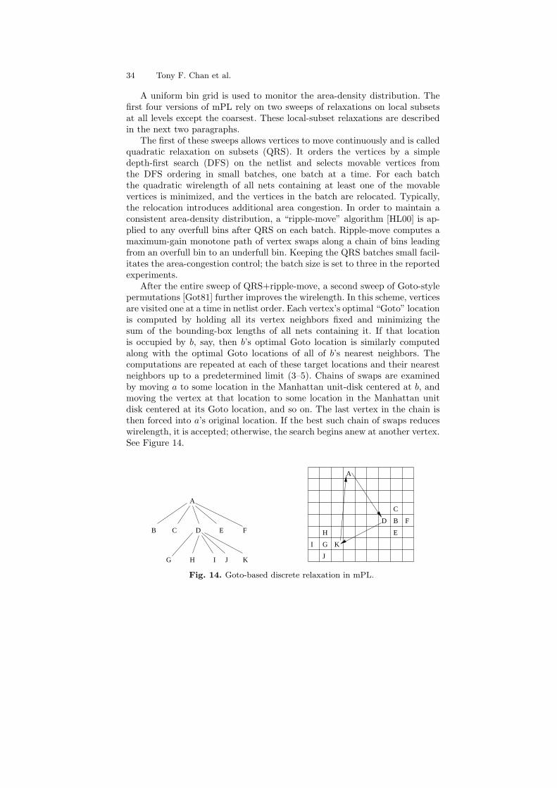
After the entire sweep of QRS+ripple-move, a second sweep of Goto-stylepermutations [Got81] further improves the wirelength. In this scheme, verticesare visited one at a time in netlist order. Each vertex’s optimal “Goto” locationis computed by holding all its vertex neighbors fixed and minimizing thesum of the bounding-box lengths of all nets containing it. If that locationis occupied by b, say, then b’s optimal Goto location is similarly computedalong with the optimal Goto locations of all of b’s nearest neighbors. Thecomputations are repeated at each of these target locations and their nearestneighbors up to a predetermined limit (3–5). Chains of swaps are examinedby moving a to some location in the Manhattan unit-disk centered at b, andmoving the vertex at that location to some location in the Manhattan unitdisk centered at its Goto location, and so on. The last vertex in the chain isthen forced into a’s original location. If the best such chain of swaps reduceswirelength, it is accepted; otherwise, the search begins anew at another vertex.See Figure 14.
A
B C D E F
G H I J K
A
B
C
D
E
F
G
H
I
J
K
Fig. 14. Goto-based discrete relaxation in mPL.
Multiscale Optimization in VLSI Physical Design Automation 35
In the most recent implementation of mPL [CCS05], global relaxations,in which all movable objects are simultaneously displaced, have been scalablyincorporated at every level of hierarchy. The redistribution of smoothed areadensity is formulated as a Helmholtz equation subject to Neumann boundaryconditions, the bins defining area-density constraints serving as a discretiza-tion. A log-sum-exp smoothing of half-perimeter wirelength defined in Section3.4.2 below is the objective. Given an initial unconstrained solution at thecoarsest level or an interpolated solution at finer levels, an Uzawa method isused to iteratively improve the configuration.
Interpolation
AMG-based weighted aggregation [BHM00], in which each vertex may befractionally assigned to several generalized aggregates rather than to just onecluster, has yet to be successfully applied in the hypergraph context. Theobstacle is that it is not known how to transfer the finer-level hyperedges,objectives, and constraints accurately to the coarser level in this case. AMG-based weighted disaggregation is simpler, however, it has been successfullyapplied to placement in mPL.
For each cluster at the coarser level, a C-point representative is selectedfrom it as the vertex largest in area among those of maximal weighted hyper-edge degree. C-points simply inherit their parent clusters’ positions and serveas fixed anchors. The remaining vertices, called F-points, are ordered by non-increasing weighted hyperedge degree and placed at the weighted average oftheir strong C-point neighbors and strong, already-placed F-point neighbors.This F-point repositioning is iterated a few times, but the C-points are heldfixed all the while.
Iteration Flow
Two backtracking V-cycles are used (Figure 8). The first follows the connect-ivity-based FC clustering hierarchy described above. The second follows asimilar FC-cluster hierarchy in which both connectivity and proximity areused to calculate vertex affinities:
rij =∑
{e∈E | i,j∈e}
w(e)
(|e| − 1)area(e)||(xi, yi)− (xj , yj)||.
During this second aggregation, positions are preserved by placing clustersat the weighted average of their component vertices’ positions. No nonlinearprogramming is used in the second cycle, because it alters the initial placementtoo much and degrades the final result.
36 Tony F. Chan et al.
3.3.3 mPG
As described in Section 4, the wires implementing netlist connections areplaced not only in the same region containing circuit cells, but also in a setof 3–12 routing layers directly above the placement region. The bottom layersclosest to the cells are used for the shortest connections. The top layers areused for global connections. These can be made faster by increasing wirewidths and wire spacing. As circuit sizes continue to increase, so do both thenumber of layers and the competition for wiring paths at the top layers. Overhalf the wires in a recent microprocessor design are over 0.5 mm in length,while only 4.1% are below 0.5 mm in length [CCPY02].
While many simple, statistical methods for estimating routing conges-tion during placement exist (topology-free congestion estimation [LTKS02])it is generally believed that, for a placement algorithm to consistently pro-duce routable results, some form of approximate routing topology mustbe explicitly constructed during placement as a guide. The principal goalof mPG [CCPY02] is to incorporate fast, constructive routing-congestionestimates, including layer assignment, into a wirelength-driven, simulated-annealing based multiscale placement engine. Compared to Gordian-L [SDJ91],mPG is 4–6.7 times faster and generates slightly better wirelength for test cir-cuits with more than 100,000 cells. In congestion-driven mode, mPG reduceswiring overflow estimates by 45%–74%, with a 5% increase in wirelength com-pared to wirelength-driven mode, but 3–7% less wirelength after global rout-ing. The results of the mPG experiments show that the multiscale placementframework is readily adapted to incorporate complex routability constraintseffectively.
Hierarchy construction
mPG uses connectivity-driven, recursive first-choice clustering (FC, Section2.2.1) to build its placement hierarchy on the netlist. The vertex affinity usedto define clusters is similar to that used by mPL, as defined in (3). However,instead of matching a given vertex to its highest-affinity neighbor, mPG selectsa neighbor at random from the those in the top 10% affinity. Moreover, themPG vertex affinity does not consider vertex area. Experiments for mPGshow that imposing explicit constraints on cluster areas in order to limitthe cluster-area variation increases run time without significantly improvingplacement quality. The strategy in mPG is instead to allow unlimited variationin cluster areas, thereby reducing the number of cluster levels and allowingmore computation time at each level.
Large variations in cluster sizes are managable in mPG due to its hier-archical area-density model. Optimization at each level of the netlist-clusterhierarchy is performed over the exact same set of regular, uniform, nestedbin-density grids. By gradually reducing the area overflow in bins at all scalesfrom the size of the smallest cells up to 1/4 the placement region, a sufficiently
Multiscale Optimization in VLSI Physical Design Automation 37
uniform distribution of cell areas is obtained for detailed placement. The samegrid hierarchy is also used to perform fast incremental, global routing, includ-ing fast layer assignment, and to estimate routing congestion in each bin.In wirelength mode, the mPG objective is simply bounding-box wirelength,as in (1). In (routability) congestion mode, the objective is equivalent to aweighted-wirelength version of (1), in which the weight of a net is propor-tional to the sum of the estimated wire usages of the bins used by that net’srectilinear Steiner-tree routing. The congestion-based objective is used onlyat finer levels of the cluster hierarchy.
Relaxation
Relaxation in mPG is by simulated annealing. Throughout the process, ver-tices are positioned only at bin centers. All vertex moves are discrete, from onebin center to another. At each step, a cluster is randomly selected. A targetlocation for the cluster is then selected either (a) randomly within some rangelimit or (b) to minimize the total bounding-box wirelength of the nets contain-ing it. The probability of selecting the target randomly is set to max{α, 0.6},where α is the “acceptance ratio.” The probability p of accepting a move withcost change ∆C is one if ∆C ≤ 0 and exp{−∆C/T} if ∆C > 0, where Tdenotes the temperature. At the coarsest level k, the starting temperature isset to approximately 20 times the standard deviation of the cost changes ofnk random moves, where ni denotes the number of clusters at level i. At otherlevels, binary search is used to estimate a temperature for which the expectedcost change is zero. These approximate “equilibrium temperatures” are usedas starting temperatures for those levels.
When accepting a move to a target location results in a density-constraintviolation, an alternative location near the target can be found efficiently, if itexists, by means of the hierarchical bin-density structure.
Annealing proceeds at a given temperature in sweeps of ni vertex movesas long as the given objective can be decreased. After a certain number ofconsecutive sweeps with net increase in the objective, the temperature is de-creased by a factor µ = µ(α), in a manner similar to that used by UltrafastVPR. The default stopping temperature is taken to be 0.005C/|E|, where Cis the objective value and |E| is the number of nets at the current level.
Interpolation
Cluster components are placed concentrically at the cluster center.
Iteration Flow
One V-cycle is used: recursive netlist coarsening followed by one recursiveinterpolation pass from the coarsest to the finest level. Relaxation is used ateach level only in the interpolation pass.
38 Tony F. Chan et al.
3.4 Partitioning-based Methods
An apparent deficiency with clustering-based hierarchies is that, while they areobserved to perform well on circuits that can be placed with mostly short, localconnections, they may be less effective for circuits that necessarily contain ahigh proportion of relative long, global connections. A bottom-up approachto placement may not work well on a design formed from the top down.
A placement hierarchy can also be constructed from the top down in aneffort to better capture the global interconnections of a design. An aggregateneed not be defined by recursive clustering; recursive circuit partitioning (Sec-tion 2) can be used instead. In this approach, the coarsest level is defined firstas just two (or perhaps four) partition blocks. Each placement level is ob-tained from its coarser neighboring level by partitioning the partition blocksat that coarser level.
Although partitioning’s use as a means of defining a hierarchy for multi-scale placement is relatively new, placement by recursive partitioning has along tradition. The average number of interconnections between subregionsis obviously correlated with total wirelength. A good placement can there-fore be viewed as one requiring as few interconnections as possible betweensubregions.
Minimizing cutsize is generally acknowledged as easier than placement,and, since the arrival of multiscale hypergraph partitioners hMetis and ML-part (Sections 2.2 and 2.3), little or no progress in partitioning tools hasbeen made. Partitioning tools are thus generally seen as more mature thanplacement tools, whose development continues to progress rapidly. Placementalgorithms based on partitioning gain some leverage from the superior perfor-mance of the state-of-the-art partitioning tools.
3.4.1 Dragon
Since its introduction in 2000 [WYS00b], Dragon has become a standardfor comparison among academic placers for the low wirelength and highroutability of the placements it generates. Dragon combines a partitioning-based cutsize-driven optimization with wirelength-driven simulated annealingon partition blocks to produce placements at each level. Like mPG and Ul-trafast VPR, Dragon relies on simulated annealing as its principal meansof intralevel iterative improvement. Unlike these algorithms, Dragon’s hier-archy is ultimately defined by top-down recursive partitioning rather thanrecursive clustering. Heavy reliance on annealing slows Dragon’s performancerelative to other techniques and may diminish its scalability somewhat (Sec-tion 1.5). The flexibility, simplicity, and power of the annealing-based ap-proach, however, makes Dragon adaptable to a variety of problem formula-tions [SWY02, XWCS03].
Multiscale Optimization in VLSI Physical Design Automation 39
Hierarchy construction
Dragon’s placement hierarchy is built from the top down. Initially, a cutsize-driven quadrisection of the circuit is computed by hMetis (Section 2.2). Eachof the four partition blocks is then viewed as an aggregate. The aggregate isgiven an area in proportion to its cell content, and the cells within each suchaggregate are placed at the aggregate’s center. Half-perimeter wirelength--driven annealing on these aggregates is then used to determine their relativelocations in the placement region. Cutsize-driven quadrisection is then ap-plied to each of the aggregates, producing 16 = 4× 4 aggregates at the nextlevel. Wirelength-driven annealing then determines positions of these new,smaller aggregates within some limited distance of their parent aggregates’locations. This sequence of cutsize-driven subregion quadrisection followed bywirelength-driven positioning continues until the number of cells in each par-titioning block is approximately 7. At that point, greedy heuristics are usedto obtain a final, overlap free placement.
When a given partition block Bi is quadrisected, the manner in whichits connections to other partition blocks Bj at the same level are modeledmay have considerable impact. In standard non-multiscale approaches, vari-ous forms of terminal propagation (Section 3.2) are the most effective knowntechnique. Experiments reported by Dragon’s authors indicate, however, thatterminal propagation is inappropriate in the multiscale setting, where en-tire partition blocks are subsequently moved. Among a variety of attemptedstrategies, the one ultimately selected for Dragon is simply to replace anynet containing cells in both Bi and other partition blocks by the cells in Bicontained by that net. Thus, during quadrisection, all connections within Biare preserved, but connections to external blocks are ignored. Connectionsbetween blocks are accurately modeled only during the relaxation phase de-scribed below.
Although hMetis is a multiscale partitioner and therefore generates its ownhierarchy by recursive clustering, Dragon makes no explicit use of hMetis’sclustering hierarchy it its top-down phase. Instead, Dragon uses the final resultof the partitioner as a means of defining a new hierarchy from the top down.It is this top-down, partitioning-based hierarchy which defines the placementproblems to which Dragon’s wirelength-driven relaxations are applied.
Relaxation
Low-temperature wirelength-driven simulated annealing is used to performpairwise swaps of nearby partition blocks. These blocks are not required toremain within the boundaries of their parent blocks. Thus, relaxation at finerlevels can to some extent correct premature decisions made at earlier, coarserlevels. However, to control the run time, the range of moves that can beconsidered must be sharply limited.
40 Tony F. Chan et al.
After the final series of quadrisections, four stages proceed to a final place-ment. First, annealing based on swapping cells between partition blocks isperformed. Second, area-density balancing linear programming [CXWS03] isused. Third, cells are spread out to remove all overlap. Finally, small permu-tations of cells are greedily considered separately along horizontal and verticaldirections from randomly selected locations.
Interpolation
The top-down hierarchy construction completely determines the manner inwhich a coarse-level solution is converted to a solution at the adjacent finerlevel. First, the cutsize-driven netlist quadrisection performed by hMetis di-vides a partition-block aggregate into four equal-area subblocks. Second, theannealing-based relaxation is used to assign each subblock to a subregion.The initial assignment of subregions to subblocks is unspecified, but, due tothe distance-limited annealing that follows, it may be taken simply as a col-lection of randomly selected 4-way assignments, each of these made locallywithin each parent aggregate’s subregion. As stated above, the ultimate sub-region selected for a subblock by the annealing need not belong to the regionassociated with its parent aggregate.
Iteration Flow
Dragon’s flow proceeds top-down directly from the coarsest level to the finestlevel. Because the multiscale hierarchy is constructed from the top down, thereis no explicit bottom-up phase and thus no notion of V-cycle etc.
3.4.2 Aplace
In VLSICAD, the word “analytical” is generally used to describe optimizationtechniques relying on smooth approximations. Among these methods, force-directed algorithms [QB79, EJ98] model the hypergraph netlist as a general-ized spring system and introduce a scalar potential field for area density. Asmooth approximations to half-perimeter wirelength (1) is minimized subjectto implicit bound constraints on area-density. Regions of high cell-area densityare sources of cell-displacement force gradients, regions of low cell-area densityare sinks. The placement problem becomes a search for equilibrium states, inwhich the tension in the spring system is balanced by the area-displacementforces.
Aplace [KW04] (the ‘A’ stands for “analytic”) is essentially a multiscaleimplementation of this approach. The wirelength model for a net t consistingof pin locations(4) t = {(xi, yi) | i = 1, . . . ,deg(t)} follows a well-known log-sum-exp approximation,
(4) A pin is a point on a cell where a net is connected to the cell.
Multiscale Optimization in VLSI Physical Design Automation 41
`exp(t) = α ·(
ln(∑
exi/α) + ln(∑
e−xi/α) + ln(∑
eyi/α) + ln(∑
e−yi/α))
,
(4)where α is a smoothing parameter. To estimate area densities, uniform gridsare used. Each subregion of a grid G is called a bin (the word “cell” is reservedfor the movable subcircuits being placed). The scalar potential field φ(x, y)used to generate area-density-balancing forces is defined as a sum over cellsand bins as follows. For a single cell v at position (xv, yv) overlapping with asingle bin b centered at (xb, yb), the potential is the bell-shaped function
φv(b) = α(v)p(|xv − xb|)p(|yv − yb|),
where α(v) is selected so that∑
b∈G φv(b) = area(v), and
p(d) ≡{
1− 2d2/r2 if 0 ≤ d ≤ r/22(d− r)2/r2 if r/2 ≤ d ≤ r, (5)
and r is the radius of the potential. The potential φ at any bin b is thendefined as the sum of the potentials φv(b) for the individual cells overlappingwith that bin. Let (X, Y ) denote all positions of all cells in the placementregion R. Let |G| denote the total number of bins in grid G. Then the targetpotential for each bin is simply φ =
∑
v∈V area(v)/|G|, and the area-densitypenalty term for a current placement (X,Y ) on grid G is defined as
ψG(X,Y ) =∑
b∈G
(φ(b)− φ
)2.
For the given area density grid G, Aplace then formulates placement as theunconstrained minimization problem
minv∈V
ρ`
(∑
e∈E`exp(e)
)
+ ρψψG(X,Y )
for appropriate, grid-dependent scalar weights ρ` and ρψ. This formulation hasbeen successfully augmented in Aplace to model routing congestion, movableI/O pads, and symmetry constraints on placed objects.
Hierarchy construction
The aggregates are defined from the top down by recursive cutsize-drivenarea bipartitioning on the hypergraph netlist. The partitioning engine usedis MLpart (Section 2.3). As in Dragon, Aplace makes no attempt to reuseMLpart’s clustering hierarchy, and Aplace’s entire hierarchy of aggregates isdefined before any relaxation begins. Thus, at the start of relaxation on thecoarsest level, all the aggregates at all levels have been defined, but none hasbeen assigned a position.
42 Tony F. Chan et al.
Relaxation
Optimization at each level of Aplace proceeds by the Polak-Ribiere variant ofnonlinear conjugate gradients [NS96] with Golden-Section linesearch [GMW81].A hard iteration limit of 100 is imposed. The grid size |G|, objective weightsρ` and ρψ, wirelength smoothing parameter α (4), and area-density potentialradius r (5) are selected and adjusted at each level to guide the convergence.Bin size and α are taken proportional to the average aggregate size at thecurrent level. The potential radius r is set to 2 on most grids but is increasedto 4 at the finest grid in order to prevent oscillations in the maximum cell-areadensity of any bin. The potential weight ρψ is fixed at one. The wirelengthweight ρ` is initially set rather large and is subsequently decreased by 0.5 toescape from local minima with too much overlap. As iterations proceed, therelative weight of the area-density penalty increases, and a relatively uniformcell-area distribution is obtained.
Interpolation
When the conjugate-gradient iterations converge, simple declustering is used.The components of each aggregate are placed concentrically at the locationof the aggregate’s center. This configuration is used as the starting point forconjugate-gradient iterations at the adjacent, finer level.
Iteration Flow
As in Dragon, there is just one pass from the coarsest to the finest level.There is no bottom-up aggregation, and there are no V-cycles. After conjugategradients at the finest level, a simple Tetris-based legalizer [Hil02] is used toremove overlap in a way that tends to preserve cells’ relative orderings.
3.5 Numerical Comparison
The results of Dragon and mPL on the IBM/ISPD98 benchmarks [Alp98]are compared(5) in Figure 15 to those of two leading representatives of thetop-down partitioning-based paradigm described in Section 3.2: Capo andFeng-Shui. To illustrate the time/quality trade-offs, the figure shows scaledrun time vs. scaled total wirelength. All values have been scaled relative tothose for mPL 4. From the figure, the following conclusions can be drawn.
(i) Dragon produces the best wirelength, by 4%, but requires the most runtime, by about 2.2×.
(ii) Capo requires the least run time (by 3×) but produces the longestwirelength (by about 9%);
(iii) mPL and Feng-Shui produce the best wirelength-to-run-time tradeoff;both are competitive with Dragon in wirelength and with Capo in run time.
(5) As this chapter goes to press, no executable for Aplace is yet publicly available.
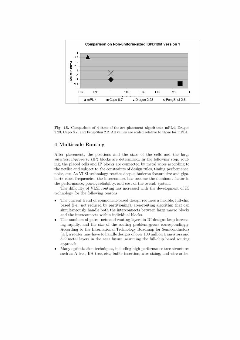
Multiscale Optimization in VLSI Physical Design Automation 43
Fig. 15. Comparison of 4 state-of-the-art placement algorithms: mPL4, Dragon2.23, Capo 8.7, and Feng-Shui 2.2. All values are scaled relative to those for mPL4.
4 Multiscale Routing
After placement, the positions and the sizes of the cells and the largeintellectual-property (IP) blocks are determined. In the following step, rout-ing, the placed cells and IP blocks are connected by metal wires according tothe netlist and subject to the constraints of design rules, timing performance,noise, etc. As VLSI technology reaches deep-submicron feature size and giga-hertz clock frequencies, the interconnect has become the dominant factor inthe performance, power, reliability, and cost of the overall system.
The difficulty of VLSI routing has increased with the development of ICtechnology for the following reasons.
• The current trend of component-based design requires a flexible, full-chipbased (i.e., not reduced by partitioning), area-routing algorithm that cansimultaneously handle both the interconnects between large macro blocksand the interconnects within individual blocks.
• The numbers of gates, nets and routing layers in IC designs keep increas-ing rapidly, and the size of the routing problem grows correspondingly.According to the International Technology Roadmap for Semiconductors[itr], a router may have to handle designs of over 100 million transistors and8–9 metal layers in the near future, assuming the full-chip based routingapproach.
• Many optimization techniques, including high-performance tree structuressuch as A-tree, BA-tree, etc.; buffer insertion; wire sizing; and wire order-
44 Tony F. Chan et al.
ing and spacing; have been proposed for high-performance circuit designs.These make the routing problem even more complicated.
In this section, we review recent efforts to apply multiscale optimizationto VLSI routing. We start with a brief introduction to the routing problemand basic techniques.
4.1 Introduction to VLSI Routing
Routing is the process of finding the geometric layouts of all the nets. Theinput of a routing problem includes the following.
routing area— the dimensions of the rectangular routing region and thenumber of available routing layers.
netlist— required interconnects as sets of connection points (“pins”) onplaced objects.
design rules— specifications of the minimum and/or maximum values al-lowed for wire width, wire spacing, via width, via spacing, etc.
pin locations— as determined by the placement or the floorplanning pro-cess.
obstacles— objects which wires cannot pass through, including placed cells,IP blocks, pads, pre-routed wires, etc.
constraint-related parameters— such as the electrical parameters (e.g.,RC constants) for performance and signal integrity constraints; thermalparameters for the thermal constraints, etc.
The constraints of a general routing process usually include connection rulesand design rules. Connection rules stipulate that (i) to prevent open circuits,wires of the same net must be connected together; and (ii) to avoid shortcircuits, wires of different nets must not overlap with each other at the samelayer. Design rules specify the sizes of the wires and vias (connections betweenlayers) and the minimum spacing between them according to the availablemanufacturing technology. The objective of the routing problem depends onthe circuit design. For general purpose chips, the objective is usually the totalwire length of all nets. For high-performance chips, the delay of the circuit isminimized. Figure 16 shows a very simple routing example with three nets.
4.2 Basic Techniques for Single Two-Pin Net Routing
In single two-pin-net routing, a path for one single net with two terminals issought. Single two-pin-net routing is a necessary component for every routingalgorithm. Basic techniques for it include maze-routing algorithms and line-probe algorithms.
The first maze-routing algorithm was proposed in 1961 by Lee [Ake67],and later on, the algorithm was improved in both time and space complex-ity [Sou78, Had75]. Lee’s basic maze-routing algorithm searches for a path
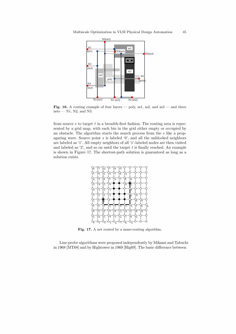
Multiscale Optimization in VLSI Physical Design Automation 45
poly
m1 N1 (m1)
N3
(m3)
N2
(m2)
N3 (m1)
N1
(poly)
m3
N3(m1)
m2
N1 (m3) N2 (m2)
N2(m2)
N2(m3)
Fig. 16. A routing example of four layers — poly, m1, m2, and m3 — and threenets — N1, N2, and N3.
from source s to target t in a breadth-first fashion. The routing area is repre-sented by a grid map, with each bin in the grid either empty or occupied byan obstacle. The algorithm starts the search process from the s like a prop-agating wave. Source point s is labeled ‘0’, and all the unblocked neighborsare labeled as ‘1’. All empty neighbors of all ‘1’-labeled nodes are then visitedand labeled as ‘2’, and so on until the target t is finally reached. An exampleis shown in Figure 17. The shortest-path solution is guaranteed as long as asolution exists.
s
t
1
1
1
1 2
2
2
2
2
2
2
3
3
3
3
3
3
3
3
3
4
4
4
4
4
4
4
4
4
4
5
5 5
5
5
5
5
5
5
5
6 6
6
6
6
6
6
6
6
6
7
7
7
7
7
7
7 7
7
7
8
8
8
8
8
8
8
8
8
8
9
9
9
9
9
9
9
9
9
9
9
Fig. 17. A net routed by a maze-routing algorithm.
Line-probe algorithms were proposed independently by Mikami and Tabuchiin 1968 [MT68] and by Hightower in 1969 [Hig69]. The basic difference between
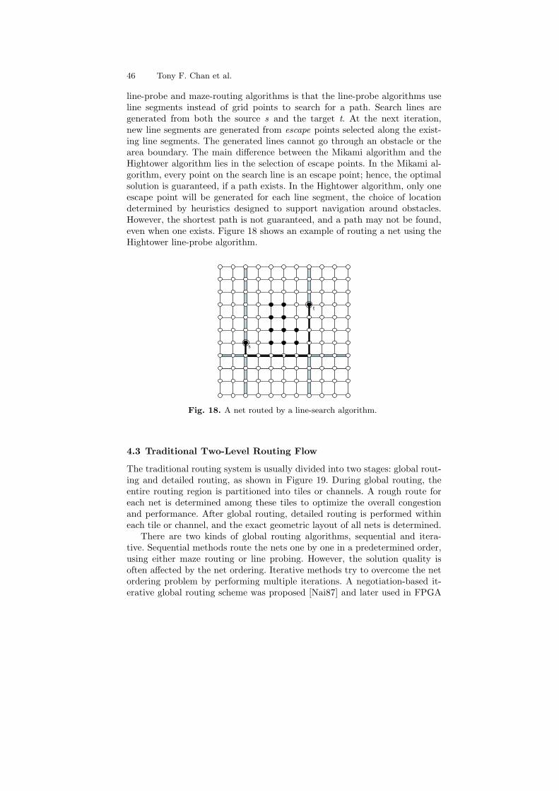
46 Tony F. Chan et al.
line-probe and maze-routing algorithms is that the line-probe algorithms useline segments instead of grid points to search for a path. Search lines aregenerated from both the source s and the target t. At the next iteration,new line segments are generated from escape points selected along the exist-ing line segments. The generated lines cannot go through an obstacle or thearea boundary. The main difference between the Mikami algorithm and theHightower algorithm lies in the selection of escape points. In the Mikami al-gorithm, every point on the search line is an escape point; hence, the optimalsolution is guaranteed, if a path exists. In the Hightower algorithm, only oneescape point will be generated for each line segment, the choice of locationdetermined by heuristics designed to support navigation around obstacles.However, the shortest path is not guaranteed, and a path may not be found,even when one exists. Figure 18 shows an example of routing a net using theHightower line-probe algorithm.
s
t
Fig. 18. A net routed by a line-search algorithm.
4.3 Traditional Two-Level Routing Flow
The traditional routing system is usually divided into two stages: global rout-ing and detailed routing, as shown in Figure 19. During global routing, theentire routing region is partitioned into tiles or channels. A rough route foreach net is determined among these tiles to optimize the overall congestionand performance. After global routing, detailed routing is performed withineach tile or channel, and the exact geometric layout of all nets is determined.
There are two kinds of global routing algorithms, sequential and itera-tive. Sequential methods route the nets one by one in a predetermined order,using either maze routing or line probing. However, the solution quality isoften affected by the net ordering. Iterative methods try to overcome the netordering problem by performing multiple iterations. A negotiation-based it-erative global routing scheme was proposed [Nai87] and later used in FPGA
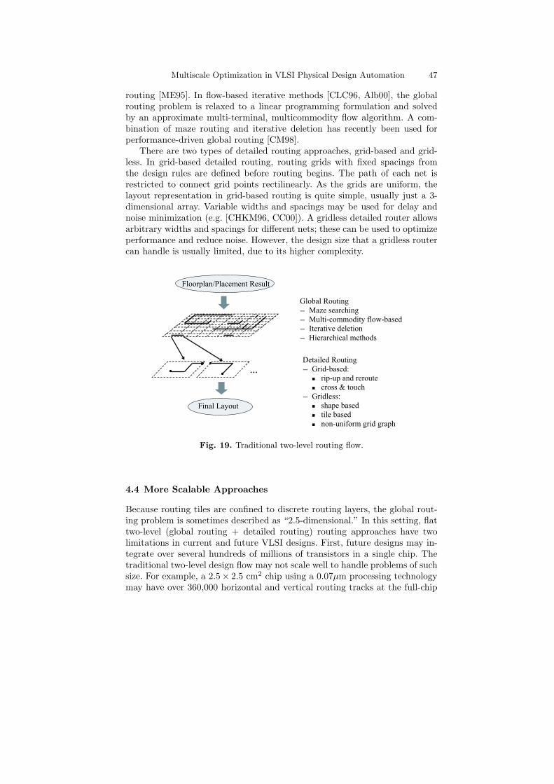
Multiscale Optimization in VLSI Physical Design Automation 47
routing [ME95]. In flow-based iterative methods [CLC96, Alb00], the globalrouting problem is relaxed to a linear programming formulation and solvedby an approximate multi-terminal, multicommodity flow algorithm. A com-bination of maze routing and iterative deletion has recently been used forperformance-driven global routing [CM98].
There are two types of detailed routing approaches, grid-based and grid-less. In grid-based detailed routing, routing grids with fixed spacings fromthe design rules are defined before routing begins. The path of each net isrestricted to connect grid points rectilinearly. As the grids are uniform, thelayout representation in grid-based routing is quite simple, usually just a 3-dimensional array. Variable widths and spacings may be used for delay andnoise minimization (e.g. [CHKM96, CC00]). A gridless detailed router allowsarbitrary widths and spacings for different nets; these can be used to optimizeperformance and reduce noise. However, the design size that a gridless routercan handle is usually limited, due to its higher complexity.
Floorplan/Placement Result
Global Routing
— Maze searching
— Multi-commodity flow-based
— Iterative deletion
— Hierarchical methods
Final Layout
…
Detailed Routing
— Grid-based:
n rip-up and reroute
n cross & touch
— Gridless:
n shape based
n tile based
n non-uniform grid graph
Fig. 19. Traditional two-level routing flow.
4.4 More Scalable Approaches
Because routing tiles are confined to discrete routing layers, the global rout-ing problem is sometimes described as “2.5-dimensional.” In this setting, flattwo-level (global routing + detailed routing) routing approaches have twolimitations in current and future VLSI designs. First, future designs may in-tegrate over several hundreds of millions of transistors in a single chip. Thetraditional two-level design flow may not scale well to handle problems of suchsize. For example, a 2.5× 2.5 cm2 chip using a 0.07µm processing technologymay have over 360,000 horizontal and vertical routing tracks at the full-chip
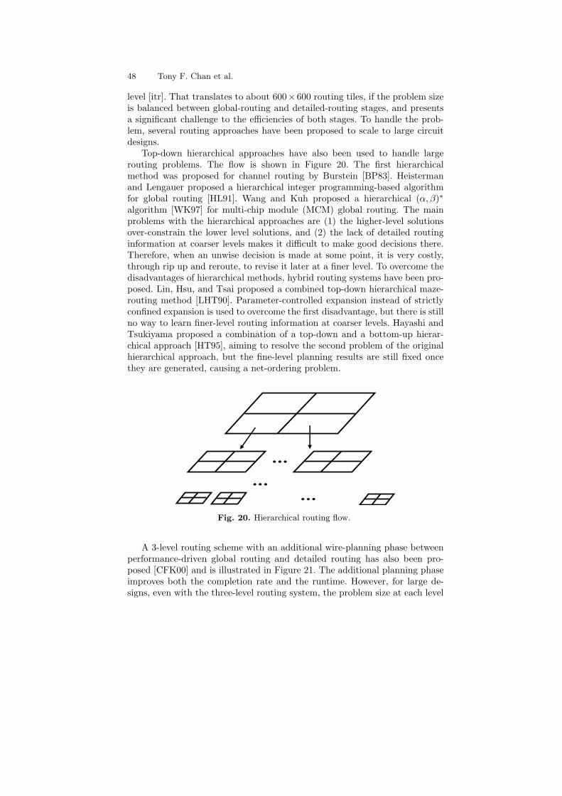
48 Tony F. Chan et al.
level [itr]. That translates to about 600×600 routing tiles, if the problem sizeis balanced between global-routing and detailed-routing stages, and presentsa significant challenge to the efficiencies of both stages. To handle the prob-lem, several routing approaches have been proposed to scale to large circuitdesigns.
Top-down hierarchical approaches have also been used to handle largerouting problems. The flow is shown in Figure 20. The first hierarchicalmethod was proposed for channel routing by Burstein [BP83]. Heistermanand Lengauer proposed a hierarchical integer programming-based algorithmfor global routing [HL91]. Wang and Kuh proposed a hierarchical (α, β)∗
algorithm [WK97] for multi-chip module (MCM) global routing. The mainproblems with the hierarchical approaches are (1) the higher-level solutionsover-constrain the lower level solutions, and (2) the lack of detailed routinginformation at coarser levels makes it difficult to make good decisions there.Therefore, when an unwise decision is made at some point, it is very costly,through rip up and reroute, to revise it later at a finer level. To overcome thedisadvantages of hierarchical methods, hybrid routing systems have been pro-posed. Lin, Hsu, and Tsai proposed a combined top-down hierarchical maze-routing method [LHT90]. Parameter-controlled expansion instead of strictlyconfined expansion is used to overcome the first disadvantage, but there is stillno way to learn finer-level routing information at coarser levels. Hayashi andTsukiyama proposed a combination of a top-down and a bottom-up hierar-chical approach [HT95], aiming to resolve the second problem of the originalhierarchical approach, but the fine-level planning results are still fixed oncethey are generated, causing a net-ordering problem.
Fig. 20. Hierarchical routing flow.
A 3-level routing scheme with an additional wire-planning phase betweenperformance-driven global routing and detailed routing has also been pro-posed [CFK00] and is illustrated in Figure 21. The additional planning phaseimproves both the completion rate and the runtime. However, for large de-signs, even with the three-level routing system, the problem size at each level
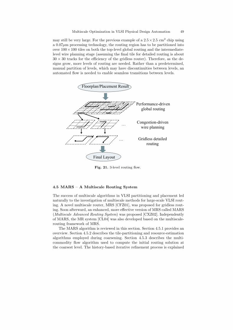
Multiscale Optimization in VLSI Physical Design Automation 49
may still be very large. For the previous example of a 2.5×2.5 cm2 chip usinga 0.07µm processing technology, the routing region has to be partitioned intoover 100×100 tiles on both the top-level global routing and the intermediate-level wire planning stage (assuming the final tile for detailed routing is about30 × 30 tracks for the efficiency of the gridless router). Therefore, as the de-signs grow, more levels of routing are needed. Rather than a predetermined,manual partition of levels, which may have discontinuities between levels, anautomated flow is needed to enable seamless transitions between levels.
Floorplan/Placement Result
Final Layout
…
…
Performance-driven
global routing
Congestion-driven
wire planning
Gridless detailed
routing
Fig. 21. 3-level routing flow.
4.5 MARS – A Multiscale Routing System
The success of multiscale algorithms in VLSI partitioning and placement lednaturally to the investigation of multiscale methods for large-scale VLSI rout-ing. A novel multiscale router, MRS [CFZ01], was proposed for gridless rout-ing. Soon afterward, an enhanced, more effective version of MRS called MARS(Multiscale Advanced Routing System) was proposed [CXZ02]. Independentlyof MARS, the MR system [CL04] was also developed based on the multiscale-routing framework of MRS.
The MARS algorithm is reviewed in this section. Section 4.5.1 provides anoverview. Section 4.5.2 describes the tile-partitioning and resource-estimationalgorithms employed during coarsening. Section 4.5.3 describes the multi-commodity flow algorithm used to compute the initial routing solution atthe coarsest level. The history-based iterative refinement process is explained
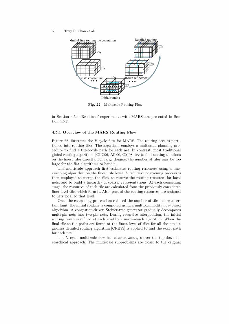
50 Tony F. Chan et al.
•Initial fine routing tile generation •Detailed routing
G1
•Tile coarsening
G0
•Route refinement
•Initial routing
Gk
Fig. 22. Multiscale Routing Flow.
in Section 4.5.4. Results of experiments with MARS are presented in Sec-tion 4.5.7.
4.5.1 Overview of the MARS Routing Flow
Figure 22 illustrates the V-cycle flow for MARS. The routing area is parti-tioned into routing tiles. The algorithm employs a multiscale planning pro-cedure to find a tile-to-tile path for each net. In contrast, most traditionalglobal-routing algorithms [CLC96, Alb00, CM98] try to find routing solutionson the finest tiles directly. For large designs, the number of tiles may be toolarge for the flat algorithms to handle.
The multiscale approach first estimates routing resources using a line-sweeping algorithm on the finest tile level. A recursive coarsening process isthen employed to merge the tiles, to reserve the routing resources for localnets, and to build a hierarchy of coarser representations. At each coarseningstage, the resources of each tile are calculated from the previously consideredfiner-level tiles which form it. Also, part of the routing resources are assignedto nets local to that level.
Once the coarsening process has reduced the number of tiles below a cer-tain limit, the initial routing is computed using a multicommodity flow-basedalgorithm. A congestion-driven Steiner-tree generator gradually decomposesmulti-pin nets into two-pin nets. During recursive interpolation, the initialrouting result is refined at each level by a maze-search algorithm. When thefinal tile-to-tile paths are found at the finest level of tiles for all the nets, agridless detailed routing algorithm [CFK99] is applied to find the exact pathfor each net.
The V-cycle multiscale flow has clear advantages over the top-down hi-erarchical approach. The multiscale subproblems are closer to the original
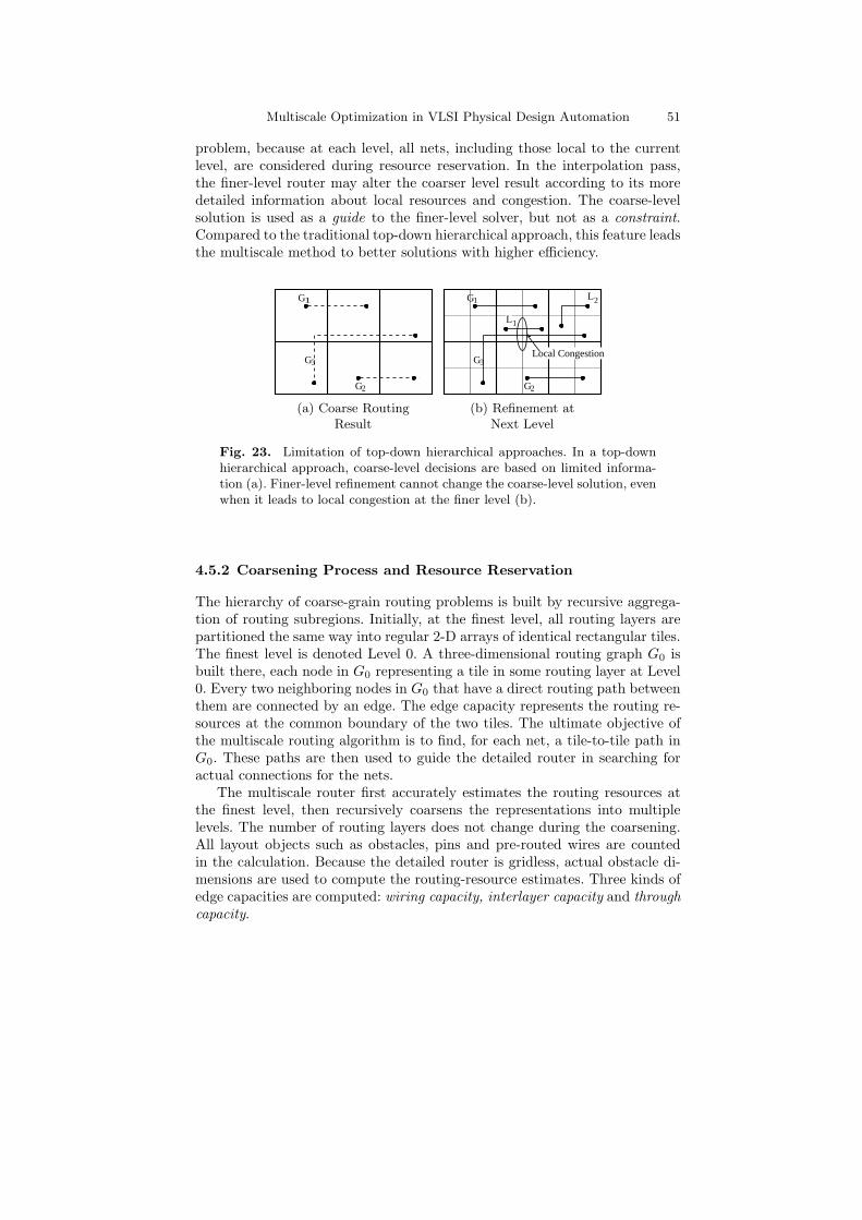
Multiscale Optimization in VLSI Physical Design Automation 51
problem, because at each level, all nets, including those local to the currentlevel, are considered during resource reservation. In the interpolation pass,the finer-level router may alter the coarser level result according to its moredetailed information about local resources and congestion. The coarse-levelsolution is used as a guide to the finer-level solver, but not as a constraint.Compared to the traditional top-down hierarchical approach, this feature leadsthe multiscale method to better solutions with higher efficiency.
G1
G3
G2
G1
G3
G2
L1
L2
Local Congestion
(a) Coarse Routing (b) Refinement atResult Next Level
Fig. 23. Limitation of top-down hierarchical approaches. In a top-downhierarchical approach, coarse-level decisions are based on limited informa-tion (a). Finer-level refinement cannot change the coarse-level solution, evenwhen it leads to local congestion at the finer level (b).
4.5.2 Coarsening Process and Resource Reservation
The hierarchy of coarse-grain routing problems is built by recursive aggrega-tion of routing subregions. Initially, at the finest level, all routing layers arepartitioned the same way into regular 2-D arrays of identical rectangular tiles.The finest level is denoted Level 0. A three-dimensional routing graph G0 isbuilt there, each node in G0 representing a tile in some routing layer at Level0. Every two neighboring nodes in G0 that have a direct routing path betweenthem are connected by an edge. The edge capacity represents the routing re-sources at the common boundary of the two tiles. The ultimate objective ofthe multiscale routing algorithm is to find, for each net, a tile-to-tile path inG0. These paths are then used to guide the detailed router in searching foractual connections for the nets.
The multiscale router first accurately estimates the routing resources atthe finest level, then recursively coarsens the representations into multiplelevels. The number of routing layers does not change during the coarsening.All layout objects such as obstacles, pins and pre-routed wires are countedin the calculation. Because the detailed router is gridless, actual obstacle di-mensions are used to compute the routing-resource estimates. Three kinds ofedge capacities are computed: wiring capacity, interlayer capacity and throughcapacity.
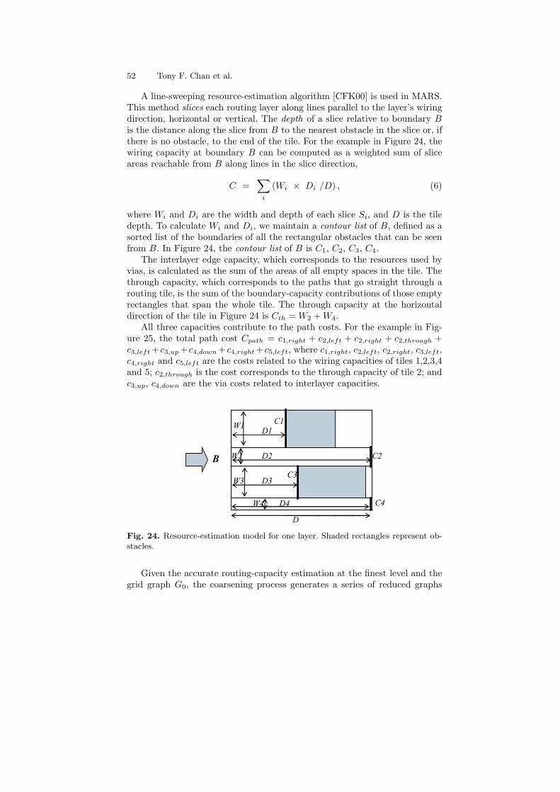
52 Tony F. Chan et al.
A line-sweeping resource-estimation algorithm [CFK00] is used in MARS.This method slices each routing layer along lines parallel to the layer’s wiringdirection, horizontal or vertical. The depth of a slice relative to boundary Bis the distance along the slice from B to the nearest obstacle in the slice or, ifthere is no obstacle, to the end of the tile. For the example in Figure 24, thewiring capacity at boundary B can be computed as a weighted sum of sliceareas reachable from B along lines in the slice direction,
C =∑
i
(Wi × Di /D) , (6)
where Wi and Di are the width and depth of each slice Si, and D is the tiledepth. To calculate Wi and Di, we maintain a contour list of B, defined as asorted list of the boundaries of all the rectangular obstacles that can be seenfrom B. In Figure 24, the contour list of B is C1, C2, C3, C4.
The interlayer edge capacity, which corresponds to the resources used byvias, is calculated as the sum of the areas of all empty spaces in the tile. Thethrough capacity, which corresponds to the paths that go straight through arouting tile, is the sum of the boundary-capacity contributions of those emptyrectangles that span the whole tile. The through capacity at the horizontaldirection of the tile in Figure 24 is Cth = W2 +W4.
All three capacities contribute to the path costs. For the example in Fig-ure 25, the total path cost Cpath = c1,right + c2,left + c2,right + c2,through +c3,left+c3,up+c4,down+c4,right+c5,left, where c1,right, c2,left, c2,right, c3,left,c4,right and c5,left are the costs related to the wiring capacities of tiles 1,2,3,4and 5; c2,through is the cost corresponds to the through capacity of tile 2; andc3,up, c4,down are the via costs related to interlayer capacities.
W1
W2
W3
D1
D2
D3
D
C1
C2
C3
B
C4 W4 D4
Fig. 24. Resource-estimation model for one layer. Shaded rectangles represent ob-stacles.
Given the accurate routing-capacity estimation at the finest level and thegrid graph G0, the coarsening process generates a series of reduced graphs
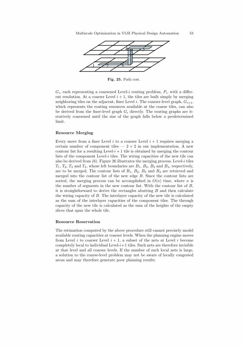
Multiscale Optimization in VLSI Physical Design Automation 53
1 2 3
4 5
Fig. 25. Path cost.
Gi, each representing a coarsened Level-i routing problem, Pi, with a differ-ent resolution. At a coarser Level i+ 1, the tiles are built simply by mergingneighboring tiles on the adjacent, finer Level i. The coarser-level graph, Gi+1,which represents the routing resources available at the coarse tiles, can alsobe derived from the finer-level graph Gi directly. The routing graphs are it-eratively coarsened until the size of the graph falls below a predeterminedlimit.
Resource Merging
Every move from a finer Level i to a coarser Level i + 1 requires merging acertain number of component tiles — 2 × 2 in our implementation. A newcontour list for a resulting Level-i+ 1 tile is obtained by merging the contourlists of the component Level-i tiles. The wiring capacities of the new tile canalso be derived from (6). Figure 26 illustrates the merging process. Level-i tilesT1, T2, T3 and T4, whose left boundaries are B1, B2, B3 and B4, respectively,are to be merged. The contour lists of B1, B2, B3 and B4 are retrieved andmerged into the contour list of the new edge B. Since the contour lists aresorted, the merging process can be accomplished in O(n) time, where n isthe number of segments in the new contour list. With the contour list of B,it is straightforward to derive the rectangles abutting B and then calculatethe wiring capacity of B. The interlayer capacity of the new tile is calculatedas the sum of the interlayer capacities of the component tiles. The throughcapacity of the new tile is calculated as the sum of the heights of the emptyslices that span the whole tile.
Resource Reservation
The estimation computed by the above procedure still cannot precisely modelavailable routing capacities at coarser levels. When the planning engine movesfrom Level i to coarser Level i + 1, a subset of the nets at Level i becomecompletely local to individual Level-i+1 tiles. Such nets are therefore invisibleat that level and all coarser levels. If the number of such local nets is large,a solution to the coarse-level problem may not be aware of locally congestedareas and may therefore generate poor planning results.
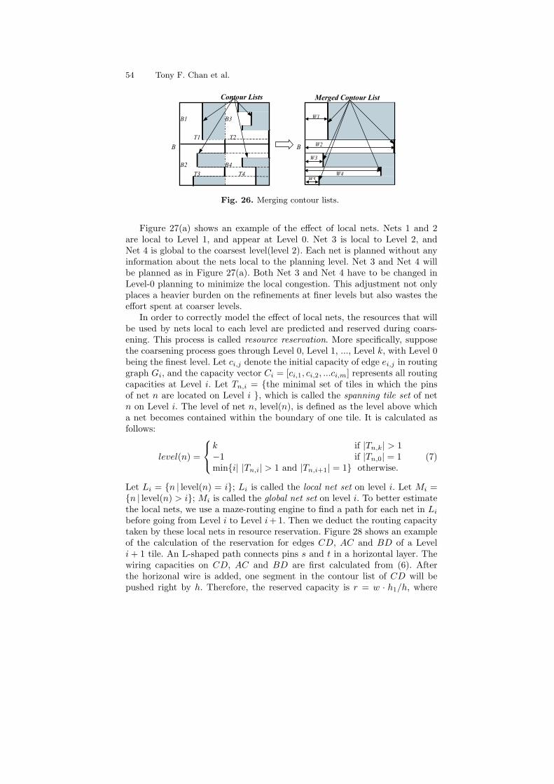
54 Tony F. Chan et al.
B4
Contour Lists
B
B1
B2
B3
T1 T2
T3 T4
B
W1
W2
W3
W4
W5
Merged Contour List
Fig. 26. Merging contour lists.
Figure 27(a) shows an example of the effect of local nets. Nets 1 and 2are local to Level 1, and appear at Level 0. Net 3 is local to Level 2, andNet 4 is global to the coarsest level(level 2). Each net is planned without anyinformation about the nets local to the planning level. Net 3 and Net 4 willbe planned as in Figure 27(a). Both Net 3 and Net 4 have to be changed inLevel-0 planning to minimize the local congestion. This adjustment not onlyplaces a heavier burden on the refinements at finer levels but also wastes theeffort spent at coarser levels.
In order to correctly model the effect of local nets, the resources that willbe used by nets local to each level are predicted and reserved during coars-ening. This process is called resource reservation. More specifically, supposethe coarsening process goes through Level 0, Level 1, ..., Level k, with Level 0being the finest level. Let ci,j denote the initial capacity of edge ei,j in routinggraph Gi, and the capacity vector Ci = [ci,1, ci,2, ...ci,m] represents all routingcapacities at Level i. Let Tn,i = {the minimal set of tiles in which the pinsof net n are located on Level i }, which is called the spanning tile set of netn on Level i. The level of net n, level(n), is defined as the level above whicha net becomes contained within the boundary of one tile. It is calculated asfollows:
level(n) =
k if |Tn,k| > 1−1 if |Tn,0| = 1min{i| |Tn,i| > 1 and |Tn,i+1| = 1} otherwise.
(7)
Let Li = {n | level(n) = i}; Li is called the local net set on level i. Let Mi ={n | level(n) > i}; Mi is called the global net set on level i. To better estimatethe local nets, we use a maze-routing engine to find a path for each net in Libefore going from Level i to Level i+ 1. Then we deduct the routing capacitytaken by these local nets in resource reservation. Figure 28 shows an exampleof the calculation of the reservation for edges CD, AC and BD of a Leveli+ 1 tile. An L-shaped path connects pins s and t in a horizontal layer. Thewiring capacities on CD, AC and BD are first calculated from (6). Afterthe horizonal wire is added, one segment in the contour list of CD will bepushed right by h. Therefore, the reserved capacity is r = w · h1/h, where
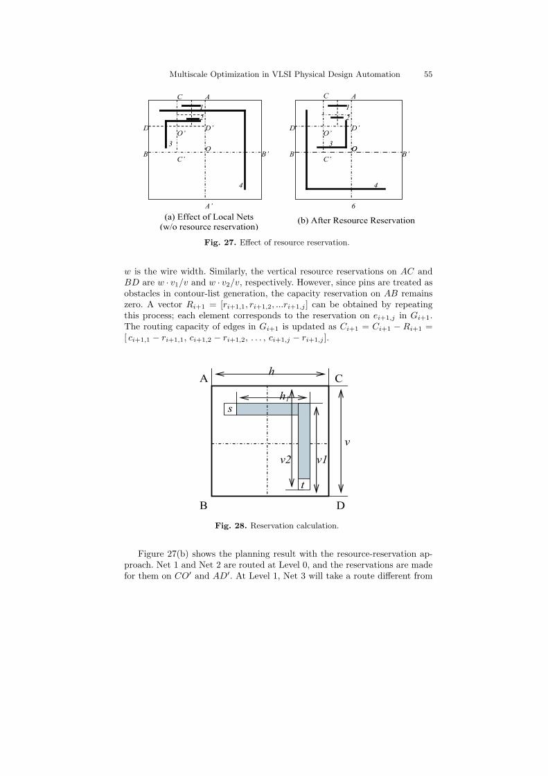
Multiscale Optimization in VLSI Physical Design Automation 55
B
D
B’
1
2
3
4
A
A’
B O
D’ D
C’
C
O’
2
3
4
1
6
A
B’ O
D’
C
C’
O’
(a) Effect of Local Nets
(w/o resource reservation) (b) After Resource Reservation
O
Fig. 27. Effect of resource reservation.
w is the wire width. Similarly, the vertical resource reservations on AC andBD are w · v1/v and w · v2/v, respectively. However, since pins are treated asobstacles in contour-list generation, the capacity reservation on AB remainszero. A vector Ri+1 = [ri+1,1, ri+1,2, ...ri+1,j ] can be obtained by repeatingthis process; each element corresponds to the reservation on ei+1,j in Gi+1.The routing capacity of edges in Gi+1 is updated as Ci+1 = Ci+1 − Ri+1 =[ ci+1,1 − ri+1,1, ci+1,2 − ri+1,2, . . . , ci+1,j − ri+1,j ].
A
h
B
h1
s
t
C
D
v
v2 v1
Fig. 28. Reservation calculation.
Figure 27(b) shows the planning result with the resource-reservation ap-proach. Net 1 and Net 2 are routed at Level 0, and the reservations are madefor them on CO′ and AD′. At Level 1, Net 3 will take a route different from
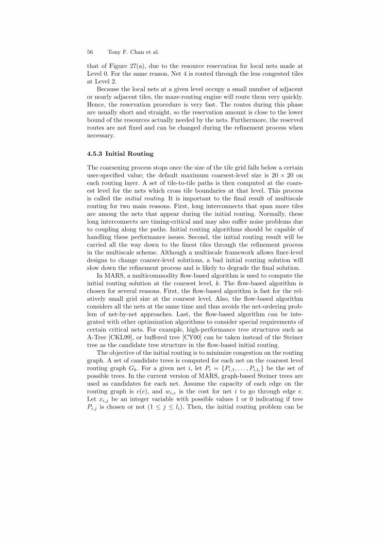
56 Tony F. Chan et al.
that of Figure 27(a), due to the resource reservation for local nets made atLevel 0. For the same reason, Net 4 is routed through the less congested tilesat Level 2.
Because the local nets at a given level occupy a small number of adjacentor nearly adjacent tiles, the maze-routing engine will route them very quickly.Hence, the reservation procedure is very fast. The routes during this phaseare usually short and straight, so the reservation amount is close to the lowerbound of the resources actually needed by the nets. Furthermore, the reservedroutes are not fixed and can be changed during the refinement process whennecessary.
4.5.3 Initial Routing
The coarsening process stops once the size of the tile grid falls below a certainuser-specified value; the default maximum coarsest-level size is 20 × 20 oneach routing layer. A set of tile-to-tile paths is then computed at the coars-est level for the nets which cross tile boundaries at that level. This processis called the initial routing. It is important to the final result of multiscalerouting for two main reasons. First, long interconnects that span more tilesare among the nets that appear during the initial routing. Normally, theselong interconnects are timing-critical and may also suffer noise problems dueto coupling along the paths. Initial routing algorithms should be capable ofhandling these performance issues. Second, the initial routing result will becarried all the way down to the finest tiles through the refinement processin the multiscale scheme. Although a multiscale framework allows finer-leveldesigns to change coarser-level solutions, a bad initial routing solution willslow down the refinement process and is likely to degrade the final solution.
In MARS, a multicommodity flow-based algorithm is used to compute theinitial routing solution at the coarsest level, k. The flow-based algorithm ischosen for several reasons. First, the flow-based algorithm is fast for the rel-atively small grid size at the coarsest level. Also, the flow-based algorithmconsiders all the nets at the same time and thus avoids the net-ordering prob-lem of net-by-net approaches. Last, the flow-based algorithm can be inte-grated with other optimization algorithms to consider special requirements ofcertain critical nets. For example, high-performance tree structures such asA-Tree [CKL99], or buffered tree [CY00] can be taken instead of the Steinertree as the candidate tree structure in the flow-based initial routing.
The objective of the initial routing is to minimize congestion on the routinggraph. A set of candidate trees is computed for each net on the coarsest levelrouting graph Gk. For a given net i, let Pi = {Pi,1, . . . , Pi,li} be the set ofpossible trees. In the current version of MARS, graph-based Steiner trees areused as candidates for each net. Assume the capacity of each edge on therouting graph is c(e), and wi,e is the cost for net i to go through edge e.Let xi,j be an integer variable with possible values 1 or 0 indicating if treePi,j is chosen or not (1 ≤ j ≤ li). Then, the initial routing problem can be
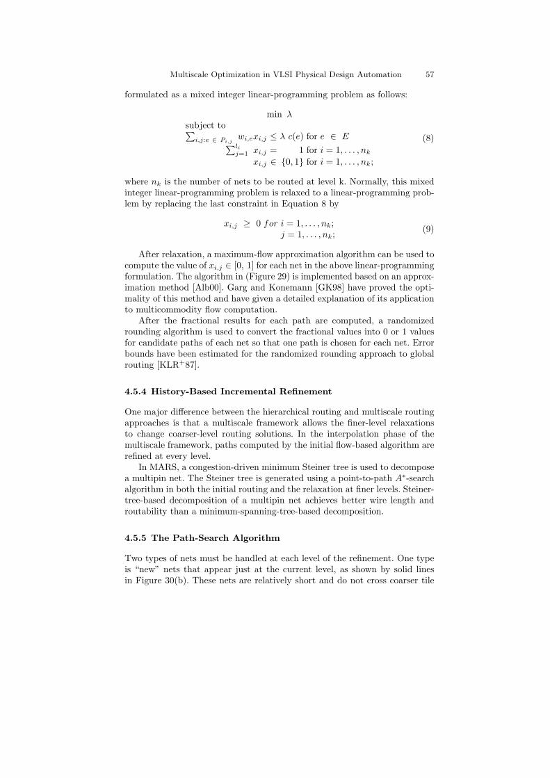
Multiscale Optimization in VLSI Physical Design Automation 57
formulated as a mixed integer linear-programming problem as follows:
min λsubject to∑
i,j:e ∈ Pi,jwi,exi,j ≤ λ c(e) for e ∈ E
∑lij=1 xi,j = 1 for i = 1, . . . , nk
xi,j ∈ {0, 1} for i = 1, . . . , nk;
(8)
where nk is the number of nets to be routed at level k. Normally, this mixedinteger linear-programming problem is relaxed to a linear-programming prob-lem by replacing the last constraint in Equation 8 by
xi,j ≥ 0 for i = 1, . . . , nk;j = 1, . . . , nk;
(9)
After relaxation, a maximum-flow approximation algorithm can be used tocompute the value of xi,j ∈ [0, 1] for each net in the above linear-programmingformulation. The algorithm in (Figure 29) is implemented based on an approx-imation method [Alb00]. Garg and Konemann [GK98] have proved the opti-mality of this method and have given a detailed explanation of its applicationto multicommodity flow computation.
After the fractional results for each path are computed, a randomizedrounding algorithm is used to convert the fractional values into 0 or 1 valuesfor candidate paths of each net so that one path is chosen for each net. Errorbounds have been estimated for the randomized rounding approach to globalrouting [KLR+87].
4.5.4 History-Based Incremental Refinement
One major difference between the hierarchical routing and multiscale routingapproaches is that a multiscale framework allows the finer-level relaxationsto change coarser-level routing solutions. In the interpolation phase of themultiscale framework, paths computed by the initial flow-based algorithm arerefined at every level.
In MARS, a congestion-driven minimum Steiner tree is used to decomposea multipin net. The Steiner tree is generated using a point-to-path A∗-searchalgorithm in both the initial routing and the relaxation at finer levels. Steiner-tree-based decomposition of a multipin net achieves better wire length androutability than a minimum-spanning-tree-based decomposition.
4.5.5 The Path-Search Algorithm
Two types of nets must be handled at each level of the refinement. One typeis “new” nets that appear just at the current level, as shown by solid linesin Figure 30(b). These nets are relatively short and do not cross coarser tile
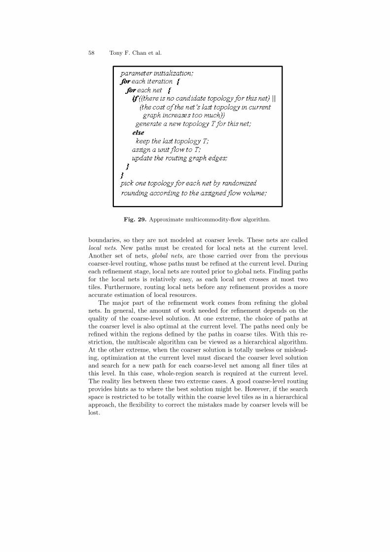
58 Tony F. Chan et al.
Fig. 29. Approximate multicommodity-flow algorithm.
boundaries, so they are not modeled at coarser levels. These nets are calledlocal nets. New paths must be created for local nets at the current level.Another set of nets, global nets, are those carried over from the previouscoarser-level routing, whose paths must be refined at the current level. Duringeach refinement stage, local nets are routed prior to global nets. Finding pathsfor the local nets is relatively easy, as each local net crosses at most twotiles. Furthermore, routing local nets before any refinement provides a moreaccurate estimation of local resources.
The major part of the refinement work comes from refining the globalnets. In general, the amount of work needed for refinement depends on thequality of the coarse-level solution. At one extreme, the choice of paths atthe coarser level is also optimal at the current level. The paths need only berefined within the regions defined by the paths in coarse tiles. With this re-striction, the multiscale algorithm can be viewed as a hierarchical algorithm.At the other extreme, when the coarser solution is totally useless or mislead-ing, optimization at the current level must discard the coarser level solutionand search for a new path for each coarse-level net among all finer tiles atthis level. In this case, whole-region search is required at the current level.The reality lies between these two extreme cases. A good coarse-level routingprovides hints as to where the best solution might be. However, if the searchspace is restricted to be totally within the coarse level tiles as in a hierarchicalapproach, the flexibility to correct the mistakes made by coarser levels will belost.
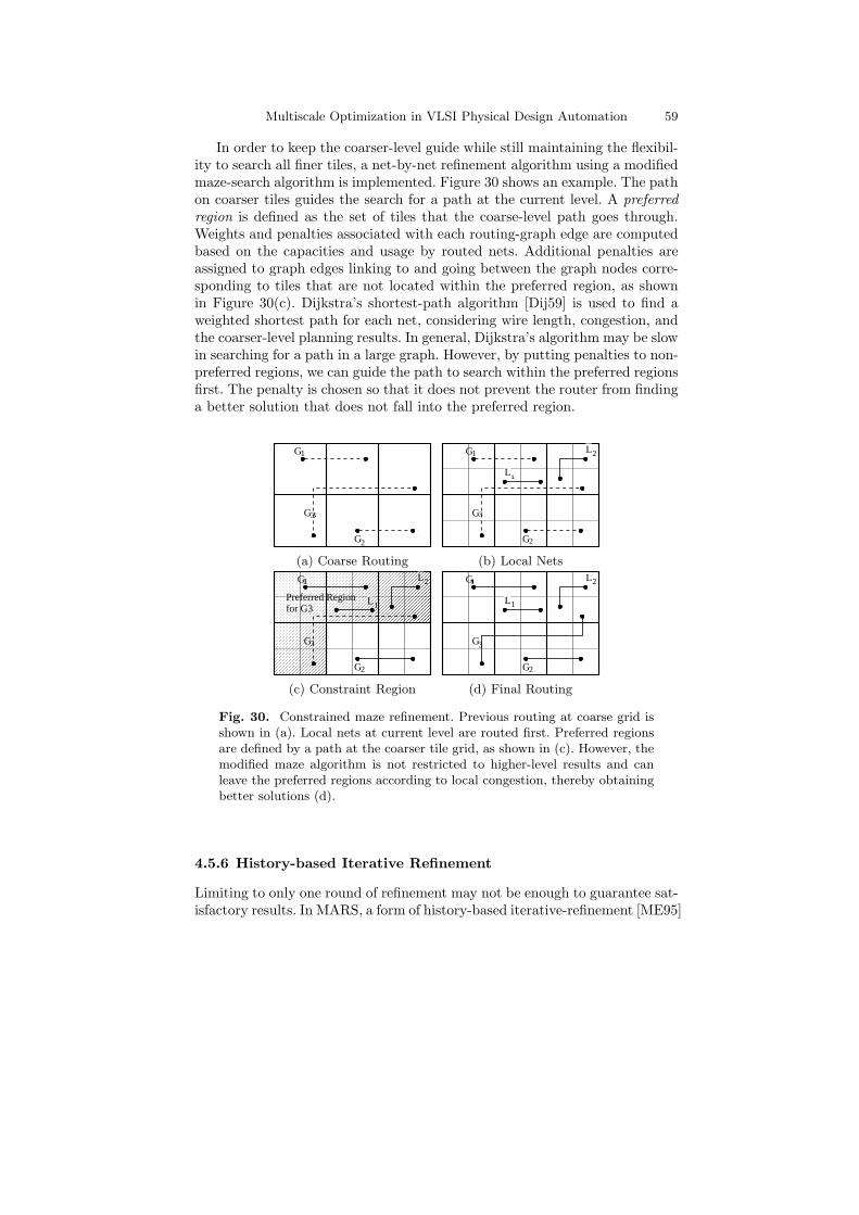
Multiscale Optimization in VLSI Physical Design Automation 59
In order to keep the coarser-level guide while still maintaining the flexibil-ity to search all finer tiles, a net-by-net refinement algorithm using a modifiedmaze-search algorithm is implemented. Figure 30 shows an example. The pathon coarser tiles guides the search for a path at the current level. A preferredregion is defined as the set of tiles that the coarse-level path goes through.Weights and penalties associated with each routing-graph edge are computedbased on the capacities and usage by routed nets. Additional penalties areassigned to graph edges linking to and going between the graph nodes corre-sponding to tiles that are not located within the preferred region, as shownin Figure 30(c). Dijkstra’s shortest-path algorithm [Dij59] is used to find aweighted shortest path for each net, considering wire length, congestion, andthe coarser-level planning results. In general, Dijkstra’s algorithm may be slowin searching for a path in a large graph. However, by putting penalties to non-preferred regions, we can guide the path to search within the preferred regionsfirst. The penalty is chosen so that it does not prevent the router from findinga better solution that does not fall into the preferred region.
G1
G3
G2
G1
G3
G2
L1
L2
(a) Coarse Routing (b) Local Nets
G1
G3
G2
L1
L2
Preferred Regionfor G3
G1
G3
G2
L1
L2
(c) Constraint Region (d) Final Routing
Fig. 30. Constrained maze refinement. Previous routing at coarse grid isshown in (a). Local nets at current level are routed first. Preferred regionsare defined by a path at the coarser tile grid, as shown in (c). However, themodified maze algorithm is not restricted to higher-level results and canleave the preferred regions according to local congestion, thereby obtainingbetter solutions (d).
4.5.6 History-based Iterative Refinement
Limiting to only one round of refinement may not be enough to guarantee sat-isfactory results. In MARS, a form of history-based iterative-refinement [ME95]
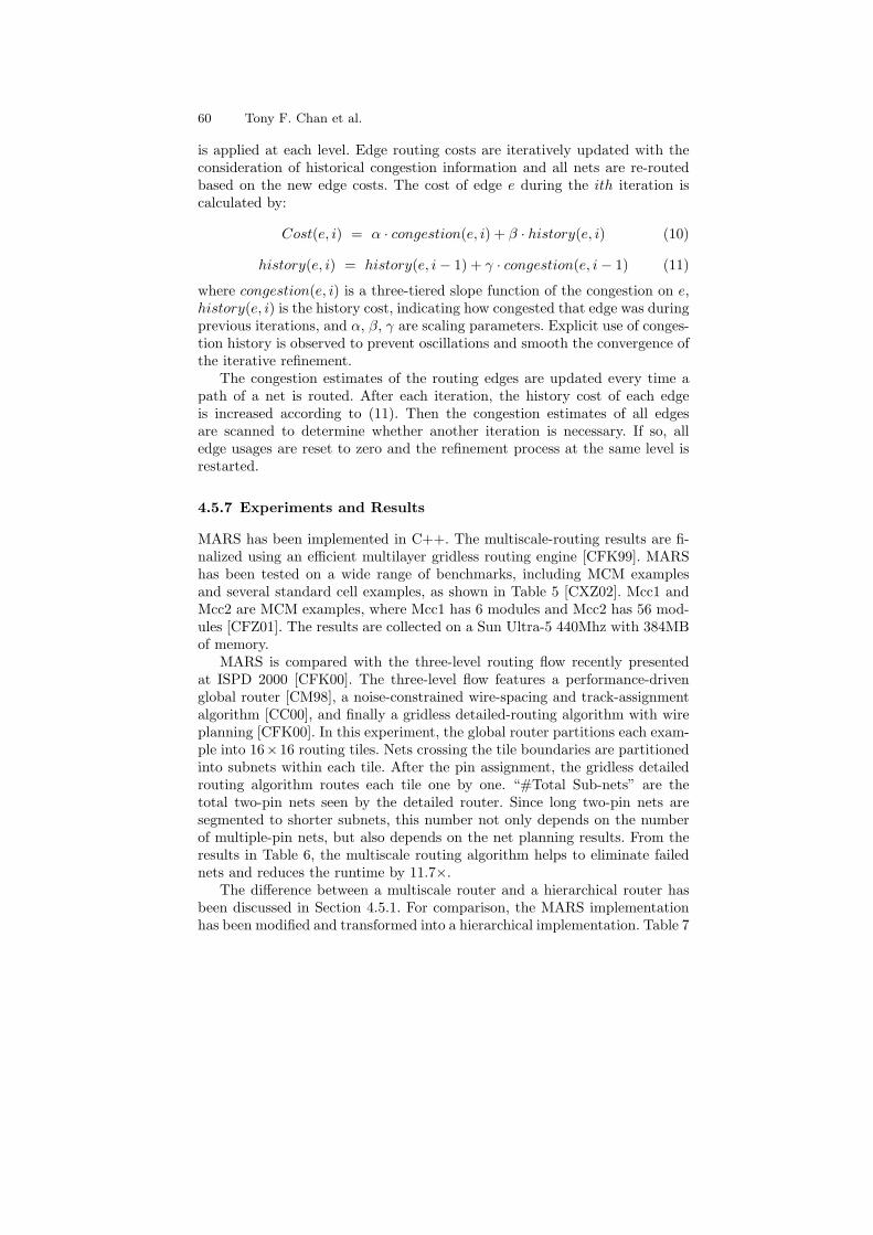
60 Tony F. Chan et al.
is applied at each level. Edge routing costs are iteratively updated with theconsideration of historical congestion information and all nets are re-routedbased on the new edge costs. The cost of edge e during the ith iteration iscalculated by:
Cost(e, i) = α · congestion(e, i) + β · history(e, i) (10)
history(e, i) = history(e, i− 1) + γ · congestion(e, i− 1) (11)
where congestion(e, i) is a three-tiered slope function of the congestion on e,history(e, i) is the history cost, indicating how congested that edge was duringprevious iterations, and α, β, γ are scaling parameters. Explicit use of conges-tion history is observed to prevent oscillations and smooth the convergence ofthe iterative refinement.
The congestion estimates of the routing edges are updated every time apath of a net is routed. After each iteration, the history cost of each edgeis increased according to (11). Then the congestion estimates of all edgesare scanned to determine whether another iteration is necessary. If so, alledge usages are reset to zero and the refinement process at the same level isrestarted.
4.5.7 Experiments and Results
MARS has been implemented in C++. The multiscale-routing results are fi-nalized using an efficient multilayer gridless routing engine [CFK99]. MARShas been tested on a wide range of benchmarks, including MCM examplesand several standard cell examples, as shown in Table 5 [CXZ02]. Mcc1 andMcc2 are MCM examples, where Mcc1 has 6 modules and Mcc2 has 56 mod-ules [CFZ01]. The results are collected on a Sun Ultra-5 440Mhz with 384MBof memory.
MARS is compared with the three-level routing flow recently presentedat ISPD 2000 [CFK00]. The three-level flow features a performance-drivenglobal router [CM98], a noise-constrained wire-spacing and track-assignmentalgorithm [CC00], and finally a gridless detailed-routing algorithm with wireplanning [CFK00]. In this experiment, the global router partitions each exam-ple into 16×16 routing tiles. Nets crossing the tile boundaries are partitionedinto subnets within each tile. After the pin assignment, the gridless detailedrouting algorithm routes each tile one by one. “#Total Sub-nets” are thetotal two-pin nets seen by the detailed router. Since long two-pin nets aresegmented to shorter subnets, this number not only depends on the numberof multiple-pin nets, but also depends on the net planning results. From theresults in Table 6, the multiscale routing algorithm helps to eliminate failednets and reduces the runtime by 11.7×.
The difference between a multiscale router and a hierarchical router hasbeen discussed in Section 4.5.1. For comparison, the MARS implementationhas been modified and transformed into a hierarchical implementation. Table 7
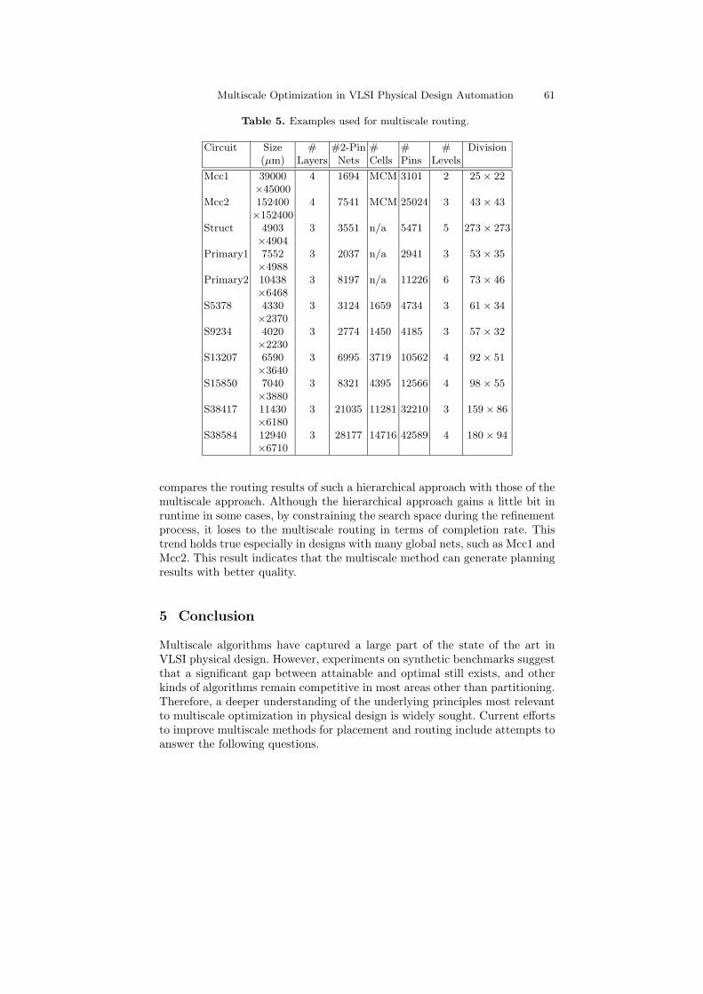
Multiscale Optimization in VLSI Physical Design Automation 61
Table 5. Examples used for multiscale routing.
Circuit Size # #2-Pin # # # Division(µm) Layers Nets Cells Pins Levels
Mcc1 39000 4 1694 MCM 3101 2 25× 22×45000
Mcc2 152400 4 7541 MCM 25024 3 43× 43×152400
Struct 4903 3 3551 n/a 5471 5 273× 273×4904
Primary1 7552 3 2037 n/a 2941 3 53× 35×4988
Primary2 10438 3 8197 n/a 11226 6 73× 46×6468
S5378 4330 3 3124 1659 4734 3 61× 34×2370
S9234 4020 3 2774 1450 4185 3 57× 32×2230
S13207 6590 3 6995 3719 10562 4 92× 51×3640
S15850 7040 3 8321 4395 12566 4 98× 55×3880
S38417 11430 3 21035 11281 32210 3 159× 86×6180
S38584 12940 3 28177 14716 42589 4 180× 94×6710
compares the routing results of such a hierarchical approach with those of themultiscale approach. Although the hierarchical approach gains a little bit inruntime in some cases, by constraining the search space during the refinementprocess, it loses to the multiscale routing in terms of completion rate. Thistrend holds true especially in designs with many global nets, such as Mcc1 andMcc2. This result indicates that the multiscale method can generate planningresults with better quality.
5 Conclusion
Multiscale algorithms have captured a large part of the state of the art inVLSI physical design. However, experiments on synthetic benchmarks suggestthat a significant gap between attainable and optimal still exists, and otherkinds of algorithms remain competitive in most areas other than partitioning.Therefore, a deeper understanding of the underlying principles most relevantto multiscale optimization in physical design is widely sought. Current effortsto improve multiscale methods for placement and routing include attempts toanswer the following questions.
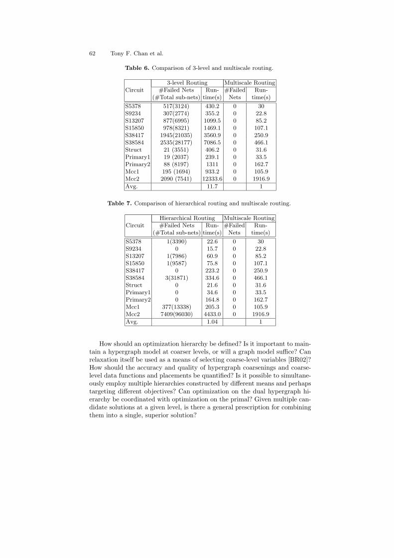
62 Tony F. Chan et al.
Table 6. Comparison of 3-level and multiscale routing.
3-level Routing Multiscale RoutingCircuit #Failed Nets Run- #Failed Run-
(#Total sub-nets) time(s) Nets time(s)
S5378 517(3124) 430.2 0 30S9234 307(2774) 355.2 0 22.8S13207 877(6995) 1099.5 0 85.2S15850 978(8321) 1469.1 0 107.1S38417 1945(21035) 3560.9 0 250.9S38584 2535(28177) 7086.5 0 466.1Struct 21 (3551) 406.2 0 31.6Primary1 19 (2037) 239.1 0 33.5Primary2 88 (8197) 1311 0 162.7Mcc1 195 (1694) 933.2 0 105.9Mcc2 2090 (7541) 12333.6 0 1916.9
Avg. 11.7 1
Table 7. Comparison of hierarchical routing and multiscale routing.
Hierarchical Routing Multiscale RoutingCircuit #Failed Nets Run- #Failed Run-
(#Total sub-nets) time(s) Nets time(s)
S5378 1(3390) 22.6 0 30S9234 0 15.7 0 22.8S13207 1(7986) 60.9 0 85.2S15850 1(9587) 75.8 0 107.1S38417 0 223.2 0 250.9S38584 3(31871) 334.6 0 466.1Struct 0 21.6 0 31.6Primary1 0 34.6 0 33.5Primary2 0 164.8 0 162.7Mcc1 377(13338) 205.3 0 105.9Mcc2 7409(96030) 4433.0 0 1916.9
Avg. 1.04 1
How should an optimization hierarchy be defined? Is it important to main-tain a hypergraph model at coarser levels, or will a graph model suffice? Canrelaxation itself be used as a means of selecting coarse-level variables [BR02]?How should the accuracy and quality of hypergraph coarsenings and coarse-level data functions and placements be quantified? Is it possible to simultane-ously employ multiple hierarchies constructed by different means and perhapstargeting different objectives? Can optimization on the dual hypergraph hi-erarchy be coordinated with optimization on the primal? Given multiple can-didate solutions at a given level, is there a general prescription for combiningthem into a single, superior solution?
Multiscale Optimization in VLSI Physical Design Automation 63
Current approaches directly optimize a coarse-level formulation of the fine-level problem. Would it be more effective at the coarser level to focus insteadon the error or displacement in the given, adjacent finer-level configuration?
Which methods of relaxation are the most effective at each level? Whatshould be the relative roles of continuous and discrete formulations? Howshould they be combined? At what point in the flow should constraints bestrictly satisfied and subsequently enforced? Are relaxations best restrictedto sequences of small subsets? How should these subsets be selected? Whenshould all variables be updated at every step?
Which is preferable: a small number of V-cycles with relatively expensiverelaxations, or a large number of V-cycles (or other hierarchy traversal) withrelatively inexpensive relaxations? Is there some underlying convergence the-ory for multiscale optimization, either to local or global solutions, that can beused to guide the practical design of the coarsening, relaxation, interpolation,and iteration flow?
As the final, physical barriers to the continuation of Moore’s Law in fab-rication technology emerge, these questions pose both a challenge and anopportunity for significant advances in VLSI physical design.
6 Acknowledgments
Funding for this work comes from Semiconductor Research Consortium Con-tracts 2003-TJ-1091 and 99-TJ-686 and National Science Foundation GrantsCCR-0096383 and CCF-0430077. The authors thank these agencies for theirsupport.
64 Tony F. Chan et al.
References
[AHK97] C. Alpert, J.-H. Huang, and A.B. Kahng. Multilevel circuit partitioning.In Proc. 34th IEEE/ACM Design Automation Conf., 1997.
[AK96] C. Alpert and A. Kahng. A hybrid multilevel/genetic approach for circuitpartitioning. In In Proceedings of the Fifth ACM/SIGDA Physical DesignWorkshop, pages 100–105, 1996.
[Ake67] S.B. Akers. A modification of Lee’s path connection algorithm. IEEETrans. on Computers, EC-16:97–98, Feb. 1967.
[Alb00] Christoph Albrecht. Provably good global routing by a new approxima-tion algorithm for multicommodity flow. In Proc. International Sympo-sium on Physical Design, pages 19–25, Mar. 2000.
[Alp98] C.J. Alpert. The ISPD98 circuit benchmark suite. In Proc. Intl Sympo-sium on Physical Design, pages 80–85, 1998.
[BHM00] W.L. Briggs, V.E. Henson, and S.F. McCormick. A Multigrid Tutorial.SIAM, Philadelphia, second edition, 2000.
[BP83] M. Burstein and R. Pelavin. Hierarchical channel router. Proc. of 20thDesign Automation Conference, pages 519–597, 1983.
[BR97] V. Betz and J. Rose. VPR: A new packing, placement, and routing toolfor FPGA research. In Proc. Intl. Workshop on FPL, pages 213–222,1997.
[BR02] A. Brandt and D. Ron. Multigrid Solvers and Multilevel OptimizationStrategies, chapter 1 of Multilevel Optimization and VLSICAD. KluwerAcademic Publishers, Boston, 2002.
[BR03] U. Brenner and A. Rohe. An effective congestion-driven placementframework. IEEE Trans. on Computer-Aided Design of Integrated Cir-cuits and Systems, 22(4):387–394, April 2003.
[Bra77] A. Brandt. Multi-level adaptive solutions to boundary value problems.Mathematics of Computation, 31(138):333–390, 1977.
[Bra86] A. Brandt. Algebraic multigrid theory: The symmetric case. Appl. Math.Comp., 19:23–56, 1986.
[Bra01] A. Brandt. Multiscale scientific computation: Review 2001. In T. Barth,R. Haimes, and T. Chan, editors, Multiscale and Multiresolution Meth-ods. Springer Verlag, 2001.
[Bre77] M.A. Breuer. Min-cut placement. J. Design Automation and Fault Tol-erant Comp., 1(4):343–362, Oct 1977.
[Cad99] Cadence Design Systems Inc. Envisia ultra placer reference.In http://www.cadence.com, QPlace version 5.1.55, compiled on10/25/1999.
[CAM00] A.E. Caldwell, A.B.Kahng, and I.L. Markov. Improved algorithms forhypergraph partitioning. In Proc. IEEE/ACM Asia South Pacific DesignAutomation Conf., 2000.
[CC00] C. Chang and J. Cong. Pseudo pin assignment with crosstalk noisecontrol. In Proc. International Symposium on Physical Design, Apr 2000.
[CCK+03] T.F. Chan, J. Cong, T. Kong, J. Shinnerl, and K. Sze. An enhancedmultilevel algorithm for circuit placement. In Proc. IEEE InternationalConference on Computer Aided Design, San Jose, CA, Nov 2003.
[CCKS00] T.F. Chan, J. Cong, T. Kong, and J. Shinnerl. Multilevel optimizationfor large-scale circuit placement. In Proc. IEEE International Conferenceon Computer Aided Design, pages 171–176, San Jose, CA, Nov 2000.
Multiscale Optimization in VLSI Physical Design Automation 65
[CCKS03] T.F. Chan, J. Cong, T. Kong, and J. Shinnerl. Multilevel Circuit Place-ment, chapter 4 of Multilevel Optimization in VLSICAD. Kluwer Aca-demic Publishers, Boston, 2003.
[CCPY02] C.C. Chang, J. Cong, Z. Pan, and X. Yuan. Physical hierarchy generationwith routing congestion control. In Proc. ACM International Symposiumon Physical Design, pages 36–41, San Diego, CA, Apr 2002.
[CCRX04] C. Chang, J. Cong, M. Romesis, and M. Xie. Optimality and scalabilitystudy of existing placement algorithms. IEEE Trans. on Computer-AidedDesign of Integrated Circuits and Systems, pages 537–549, 2004.
[CCS05] T.F. Chan, J. Cong, and K. Sze. Multilevel generalized force-directedmethod for circuit placement. In Proc. Int’l Symp. on Phys. Design,pages 185–192, 2005.
[CCX03a] C-C. Chang, J. Cong, and M. Xie. Optimality and scalability studyof existing placement algorithms. In Proc. Asia South Pacific DesignAutomation Conference, pages 621–627, 2003.
[CCX03b] C.C. Chang, J. Cong, and M. Xie. Optimality and scalability study ofexisting placement algorithms. In Asia South Pacific Design AutomationConference, pages 325–330, Kitakyushu, Japan, Jan 2003.
[CFK99] J. Cong, J. Fang, and K.Y. Khoo. An implicit connection graph mazerouting algorithm for ECO routing. In Proc. International Conferenceon Computer Aided Design, pages 163–167, Nov. 1999.
[CFK00] J. Cong, J. Fang, and K.Y. Khoo. DUNE: A multi-layer gridless rout-ing system with wire planning. In Proc. International Symposium onPhysical Design, pages 12–18, Apr. 2000.
[CFZ01] J. Cong, J. Fang, and Y. Zhang. Multilevel approach to full-chip grid-less routing. Proc. IEEE International Conference on Computer AidedDesign, pages 396–403, 2001.
[CHKM96] J. Cong, Lei He, C.-K. Koh, and P. Madden. Performance optimizationof VLSI interconnect layout. Intergration, the VLSI Journal, 21(1-2):1–94, 1996.
[CKL99] J. Cong, A.B. Kahng, and K.S. Leung. Efficient algorithms for theminimum shortest path Steiner arborescence problem with applicationsto VLSI physical design. IEEE Trans. on Computer-Aided Design,17(1):24–39, Jan. 1999.
[CKM00] A.E. Caldwell, A.B. Kahng, and I.L. Markov. Can recursive bisectionproduce routable placements? In Proc. 37th IEEE/ACM Design Au-tomation Conf., pages 477–482, 2000.
[CL00] J. Cong and S.K. Lim. Edge separability based circuit clustering withapplication to circuit partitioning. In Asia South Pacific Design Au-tomation Conference, Yokohama Japan, pages 429–434, 2000.
[CL04] Y. Chang and S. Lin. Mr: A new framework for multilevel full-chiprouting. IEEE Trans. on Computer Aided Design, 23(5), May 2004.
[CLC96] R.C. Carden, J. Li, and C.K. Cheng. A global router with a theoreticalbound on the optimal solution. IEEE Trans. Computer-Aided Design,15(2):208–216, Feb. 1996.
[CLW99] J. Cong, H. Li, and C. Wu. Simultaneous circuit partitioning/clusteringwith retiming for performance optimization. Proc. 36th ACM/IEEE De-sign Automation Conf., pages 460–465, Jun 1999.
66 Tony F. Chan et al.
[CLW00] J. Cong, S.K. Lim, and C. Wu. Performance-driven multi-level and mul-tiway partitioning with retiming. In Proceedings of Design AutomationConference, pages 274– 279, Los Angeles, California, Jun 2000.
[CM98] J. Cong and P. Madden. Performance driven multi-layer general arearouting for PCB/MCM designs. In Proc. 35th Design Automation Con-ference, pages 356–361, Jun 1998.
[CP68] H.R. Charney and D.L. Plato. Efficient partitioning of components. InIn Proc. of the 5th Annual Design Automation Workshop, pages 16–0 –16–21, 1968.
[CS93] J. Cong and M. Smith. A parallel bottom-up clustering algorithm withapplications to circuit partitioning in vlsi designs. In Proc. Design Au-tomation Conference, pages 755–760, San Jose, CA, 1993.
[CS03] J. Cong and J.R. Shinnerl, editors. Multilevel Optimization in VLSICAD.Kluwer Academic Publishers, Boston, 2003.
[CW02] J. Cong and C. Wu. Global clustering-based performance-driven circuitpartitioning. In Proc. Int. Symp. on Physical Design, pages 149–154,2002.
[CXWS03] B. Choi, H. Xu, M. Wang, and M. Sarrafzadeh. Flow-based cell movingalgorithm for desired cell distribution. Proc. IEEE International Con-ference on Computer Design, pages 218–225, Oct 2003.
[CXZ02] J. Cong, M. Xie, and Y. Zhang. An enhanced multilevel routing system.IEEE International Conference on Computer Aided Design, pages 51–58,2002.
[CY00] J. Cong and X. Yuan. Routing tree construction under fixed bufferlocations. In Proc. 37th Design Automation Conference, pages 379–384,Jun. 2000.
[DD97] Shantanu Dutt and Wenyong Deng. Vlsi circuit partitioning by cluster-removal using iterative improvement techniques. In Proc. Int’l Conf. onComputer-Aided Design, pages 194 – 200, 1997.
[Dij59] E.W. Dijkstra. A note on two problems in connexion with graphs. Nu-merische Mathematik, 1:269–271, 1959.
[DiM94] G. DiMicheli. Synthesis and Optimization of Digital Circuits. McGrawHill, 1994.
[Don88] W. E. Donath. Logic partitioning. Physical Design Automation in VLSIsystems, 1988.
[EJ98] H. Eisenmann and F.M. Johannes. Generic global placement and floor-planning. In Proc. 35th ACM/IEEE Design Automation Conference,pages 269–274, 1998.
[FM82] C. M. Fiduccia and R. M. Mattheyses. A linear-time heuristic for im-proving network partitions. In Proc. Design Automation Conference,pages 175–181, 1982.
[GK98] N. Garg and J. Konemann. Faster and simpler algorithms for multi-commodity flow and other fractional packing problems. In Proc. AnnualSymposium on Foundations of Computer Science, pages 300–309, Nov.1998.
[GMW81] P.E. Gill, W. Murray, and M.H. Wright. Practical Optimization. Aca-demic Press, London and New York, 1981. ISBN 0-12-283952-8.
[Goe03a] R. Goering. FPGA placement performs poorly, study says. EE Times,2003. http://www.eedesign.com/story/OEG20031113S0048.
Multiscale Optimization in VLSI Physical Design Automation 67
[Goe03b] R. Goering. IC placement benchmarks needed, researchers say. EETimes, 2003. http://www.eedesign.com/story/OEG20030410S0029.
[Goe03c] R. Goering. Placement tools criticized for hampering IC designs. EETimes, 2003. http://www.eedesign.com/story/OEG20030205S0014.
[Got81] S. Goto. An efficient algorithm for the two-dimensional placement prob-lem in electrical circuit layout. IEEE Trans. on Circuits and Systems,28(1):12–18, January 1981.
[Had75] F. Hadlock. Finding a maximum out of a planar graph in polynomialtime. SIAM Journal of Computing, 4(3):221–225, Sep. 1975.
[Hig69] D.W. Hightower. A solution to line routing problems on the continuousplane. In Proc. IEEE 6th Design Automation Workshop, pages 1–24,1969.
[Hil02] D. Hill. Method and system for high speed detailed placement of cellswithin an integrated circuit design. In US Patent 6370673, Apr 2002.
[HK72] M. Hannan and J.M. Kurtzberg. A review of the placement andquadratic assignment problems. SIMA, 14, 1972.
[HL91] J. Heisterman and T. Lengauer. The efficient solution of integer programsfor hierarchical global routing. IEEE Transactions on Computer-AidedDesign of Integrated Circuits and Systems, 10(6):748–753, Jun. 1991.
[HL99] S.-W. Hur and J. Lillis. Relaxation and clustering in a local searchframework: Application to linear placement. In Proc. ACM/IEEE DesignAutomation Conference, pages 360–366, New Orleans, LA, Jun 1999.
[HL00] S.-W. Hur and J. Lillis. Mongrel: Hybrid techniques for standard-cellplacement. In Proc. IEEE International Conference on Computer AidedDesign, pages 165–170, San Jose, CA, Nov 2000.
[HMS03a] B. Hu and M. Marek-Sadowska. Fine granularity clustering for large-scale placement problems. In Proc. Int’l Symp. on Physical Design, Apr.2003.
[HMS03b] B. Hu and M. Marek-Sadowska. Wire length prediction based clusteringand its application in placement. In Proc. Design Automation Confer-ence, Jun. 2003.
[HMS04] B. Hu and M. Marek-Sadowska. Fine granularity clustering based place-ment. IEEE Trans. on Computer-Aided Design of Integrated Circuitsand Systems, Apr. 2004.
[HT95] M. Hayashi and S. Tsukiyama. A hybrid hierarchical approach for multi-layer global routing. Proceedings of the 1995 European conference onDesign and Test, pages 492–496, Mar. 1995.
[itr] International Technology Roadmap for Semiconductors.http://public.itrs.net/ .
[JCX03] M. Romesis J. Cong and M. Xie. Optimality, scalability and stabilitystudy of partitioning and placement algorithms. In Proc. InternationalSymposium on Physical Design, 2003.
[KAKS97] G. Karypis, R. Aggarwal, V. Kumar, and S. Shekhar. Multilevel hy-pergraph partitioning: Application in VLSI domain. In Proc. 34thACM/IEEE Design Automation Conference, pages 526–529, 1997.
[Kar99] G. Karypis. Multilevel algorithms for multi-constraint hypergraph par-titioning. Technical Report 99-034, Department of Computer Science,University of Minnesota, Minneapolis, 1999.

68 Tony F. Chan et al.
[Kar02] G. Karypis. Multilevel Hypergraph Partitioning, chapter 3 of Multi-level Optimization and VLSICAD. Kluwer Academic Publishers, Boston,2002.
[KLR+87] R.M. Karp, F.T. Leighton, R.L. Rivest, C.D. Thompson, U.V. Vazirani,and V. V. Vazirani. Global wire routing in two-dimensional arrays. Al-gorithmica, 2:113–129, 1987.
[KSJA91] J.M. Kleinhans, G. Sigl, F.M. Johannes, and K.J. Antreich. Gordian:VLSI placement by quadratic programming and slicing optimization.IEEE Trans. on Computer-Aided Design, 10:356–365, 1991.
[KW04] A.B. Kahng and Q. Wang. Implementation and extensibility of an ana-lytic placer. In Proc. Int’l Symp. on Physical Design, pages 18–25, 2004.
[LHT90] Y. Lin, Y. Hsu, and F. Tsai. Hybrid routing. IEEE Transactions onComputer-Aided Design, 9(2):151–157, Feb. 1990.
[LLC95] J. Li, J. Lillis, and C. Cheng. Linear decomposition algorithm for vlsidesign applications. In Proc. Int’l Conf. on Computer-Aided Design,pages 223–228, 1995.
[LTKS02] J. Lou, S. Thakur, S. Krishnamoorthy, and H. Sheng. Estimating routingcongestion using probabilistic analysis. IEEE Trans. on Computer-AidedDesign of Integrated Circuits and Systems, 21(1):32–41, January 2002.
[ME95] L. McMurchie and C. Ebeling. Pathfinder: a negotiation-basedperformance-driven router for FPGAs. In Proc. of ACM Symposiumon Field-Programmable Gate Array, pages 111–117, Feb. 1995.
[MT68] K. Mikami and K. Tabuchi. A computer program for optimal routing ofprinted ciurcuit connectors. IFIPS Proc, H-47:1475–1478, 1968.
[Nai87] R. Nair. A simple yet effective technique for global wiring. IEEE Trans.on Computer-Aided Design, 6(2), 1987.
[NS96] S.G. Nash and A. Sofer. Linear and Nonlinear Programming. McGrawHill, New York, 1996.
[QB79] N. Quinn and M. Breuer. A force-directed component placement proce-dure for printed circuit boards. IEEE Trans. on Circuits and SystemsCAS, CAS-26:377–388, 1979.
[RDJ94] Bernhard M. Riess, Konrad Doll, and Frank M. Johannes. Partitioningvery large circuits using analytical placement techniques. In Proc. DesignAutomation Conference, pages 646 – 651, 1994.
[SDJ91] G. Sigl, K. Doll, and F.M. Johannes. Analytical placement: A linearor a quadratic objective function? In Proc. 28th ACM/IEEE DesignAutomation Conference, pages 427–432, 1991.
[She99] Naveed Sherwani. Algorithms for VLSI Physical Design Automation.Kluwer Academic Publishers, Boston, Dordrecht, London, third edition,1999.
[Sou78] J. Soukup. Fast maze router. In Proc. 15th Design Automation Confer-ence, pages 100–102, 1978.
[SR99] Y. Sankar and J. Rose. Trading quality for compile time: Ultra-fastplacement for FPGAs. In FPGA ‘99, ACM Symp. on FPGAs, pages157–166, 1999.
[SS95] W.-J. Sun and C. Sechen. Efficient and effective placement for very largecircuits. IEEE Trans. on Computer-Aided Design, pages 349–359, Mar1995.
[SWY02] M. Sarrafzadeh, M. Wang, and X. Yang. Modern Placement Techiques.Kluwer Academic Publishers, Boston, 2002.
Multiscale Optimization in VLSI Physical Design Automation 69
[TOS00] U. Trottenberg, C.W. Oosterlee, and A. Schuller. Multigrid. AcademicPress, London, 2000.
[Vyg97] Jens Vygen. Algorithms for large-scale flat placement. In Proc. 34thACM/IEEE Design Automation Conference, pages 746–751, 1997.
[WK97] Dongsheng Wang and E.S Kuh. A new timing-driven multilayer mcm/icrouting algorithm. In Proc. IEEE Multi-Chip Module Conference, pages89–94, Feb. 1997.
[WYS00a] M. Wang, X. Yang, and M. Sarrafzadeh. Dragon2000: Standard-cellplacement tool for large industry circuits. In Proc. International Con-ference on Computer-Aided Design, pages 260–264, 2000.
[WYS00b] M. Wang, X. Yang, and M. Sarrafzadeh. Dragon2000: Standard-cellplacement tool for large circuits. Proc. IEEE/ACM International Con-ference on Computer-Aided Design, pages 260–263, Apr 2000.
[XWCS03] H. Xu, M. Wang, B. Choi, and M. Sarrafzadeh. A trade-off ori-ented placement tool. Proc. IEEE/ACM International Conference onComputer-Aided Design, pages 467–471, Apr 2003.
[YM01] M.C. Yildiz and P.H. Madden. Improved cut sequences for partitioning-based placement. In Proc. Design Automation Conference, pages 776–779, 2001.