Submitted for publication to “Physical Review E”, code EP10271, version B

Multiple–relaxation–time Lattice Boltzmann Scheme for

Homogeneous Mixture Flows with External Force

Pietro Asinari

Department of Energetics, Politecnico di Torino,

Corso Duca degli Abruzzi 24, Torino, Italy

(Dated: March 31, 2008)

Abstract

A new LBM scheme for homogeneous mixture modeling, based on the multiple–relaxation–

time (MRT) formulation, which fully recovers Maxwell–Stefan diffusion model in the continuum

limit with (a) external force and (b) tunable Schmidt number, is developed. The proposed MRT

formulation is based on the theoretical basis of a recently proposed BGK-type kinetic model for gas

mixtures [P. Andries, K. Aoki and B. Perthame, JSP, Vol. 106, N. 5/6, 2002] and it substantially

extends the applicability of a scheme already proposed by the same author, which used only one

relaxation parameter. The recovered equations at macroscopic level are derived by an innovative

expansion technique, based on the Grad moment system. Some numerical simulations are reported

for the solvent test case with external force, aiming to find out the numerical ranges for the transport

coefficients which ensure acceptable accuracies. The numerical results prove a contraction of the

theoretical expectations, which are based on a strong separation among the characteristic scales.

PACS numbers: 47.11.-j, 05.20.Dd

1

I. INTRODUCTION

Recently, the lattice Boltzmann method (LBM) has been proposed as simple alternative

to solve simplified kinetic models. Starting from some pioneer works [1–3], the method has

reached a more systematic fashion [4, 5] by means of a better understanding of the connec-

tions with the continuous kinetic theory [6, 7] and by widening the set of applications, which

can benefit from this numerical technique. Depending on the considered LBM scheme and

the particular application, the final goal may be to solve the macroscopic equations recov-

ered in the continuum limit (in this case, LBM works as an alternative macroscopic solver)

and/or to catch rarefaction effects (which usually require larger computational stencils and

make LBM similar to kinetic discrete–velocity models).

When complex fluids are considered and the inter–particle interactions must be taken into

account, the discretized models derived by means of the lattice Boltzmann method may offer

some computational advantages over continuum based models, particularly for large parallel

computing. In order to appreciate the connection between the lattice Boltzmann method

and the conventional finite–difference techniques, it is useful to recognize that this method

can be considered a sub–class of the fully–Lagrangian methods [8, 9]. A more complete and

recent coverage of various previous contributions on LBM is beyond the purposes of the

present paper, but can be found in some review papers [10, 11] and some books [12–14].

In the present paper, the attention will be focused on the development of an LBM scheme

for homogeneous mixture modeling in the continuum limit. A lot of work has been performed

in recent years in order to produce reliable lattice Boltzmann models for this application.

See Ref. [15] and the bibliography therein for a complete discussion of this topic.

Among the most meaningful, an LBM scheme [16], which is very close to the Hamel

model approach [17, 18], has been recently proposed by means of a variational procedure

aiming to minimize a proper H function defined on the discrete lattice [16]. In particular,

this scheme [16] has the advantage to highlight that, when more than two components are

considered, the macroscopic equations, recovered by the model in the continuum limit and

ruling the mass transfer, should approach the macroscopic Maxwell–Stefan model, which

properly takes into account non-ideal effects (osmotic diffusion, reverse diffusion and diffu-

sion barrier), neglected by simpler Fick model. (a) Unfortunately this model consistently

recovers the Maxwell–Stefan diffusion equations in the continuum limit only within the

2

macroscopic mixture-averaged approximation [19], i.e. only if proper mixture-averaged dif-

fusion coefficients for each component are considered. (b) Moreover this model, like all

the previous ones strictly based on the Hamel model, can not satisfy the Indifferentiability

Principle [20] prescribing that, if a BGK-like equation for each component is assumed, this

set of equations should reduce to a single BGK-like equation, when mechanically identical

components are considered.

In order to fix both the previous problems, a new LBM scheme has been proposed [15].

As a theoretical basis for the development of the LBM scheme, a BGK-type kinetic model

for gas mixtures, recently proposed by Andries, Aoki and Perthame [21], was considered (in

the following referred as the AAP model). The main idea of the new LBM scheme is very

simple: the Maxwell–Stefan model can be obtained in LBM models by allowing momentum

exchange among different components according to the Maxwell–Stefan prescriptions. As

side effect, the obtained model satisfies the Indifferentiability Principle.

Even though the previous model [15] pointed in the in right direction, it was still effected

by the limit of the single–relaxation–time formulation. In particular, this does not allow

one to tune the kinematic viscosity independently on the diffusion transport coefficients and

consequently to tune the Schmidt number, i.e. the ratio between the kinematic viscosity of

the mixture and the diffusion coefficient of the single component. Clearly this reduces the

applicability of the model discussed in Ref. [15] to those cases where the average mixture

transport is substantially zero, or negligible in comparison with the diffusion phenomena.

Unfortunately many applications are characterized by a meaningful global transport, ruled

by the total pressure gradients inside the mixture [19].

Hence the goal of this paper is twofold:

• to design a multiple–relaxation–time (MRT) formulation of the already proposed

model [15] and to prove that the recovered equations at macroscopic level are con-

sistent with the Maxwell–Stefan model with external force, by means of an innovative

expansion technique based on the Grad moment system;

• to discuss the implementation of a generic external force in the numerical scheme, by

keeping it as general as possible, but compatible with the assumption of low Mach

number flows, as usual prescribed by the lattice Boltzmann schemes.

This paper is organized as follows. In Section II, the proposed multiple–relaxation–time

3

(MRT) LBM scheme is presented, the macroscopic equations are derived by means of an

innovative expansion based on the Grad moment system and finally some details for an

efficient implementation are discussed. Section III reports some numerical results for the

solvent test with external force: in particular, the numerical ranges for the Schmidt numbers

are obtained by discussing the desired accuracies with regards to the diffusion transport

coefficients. Finally, Section IV summarizes the main results of the paper.

II. MRT LATTICE BOLTZMANN SCHEME

A. AAP model with forcing

Numerous model equations are influenced by Maxwell’s approach to solve the Boltzmann

equation by using the properties of the Maxwell particles [22] and the linearized Boltzmann

equation. The simplest model equations for a binary mixture is that by Gross and Krook

[23], which is an extension of the single-relaxation-time model for a pure system, i.e. the

celebrated Bhatnagar-Gross-Krook (BGK) model [24]. A complete review of the BGK-type

kinetic models for mixtures can be found in Ref. [21] and, concerning the pseudo-kinetic

models for LBM schemes, in Ref. [25].

In this paper, we focus on the BGK-type model proposed by Andries, Aoki and Perthame

[21], which will be referred to in the following as AAP model, in case of isothermal flow,

which is enough to highlight the main features. A complete derivation and discussion of the

LBM scheme based on the AAP model without external forcing and with elementary single-

relaxation-time formulation can be found in Ref. [15]. The model shows some interesting

theoretical features, in particular in terms of satisfying the Indifferentiability Principle and

fully recovering the macroscopic Maxwell–Stefan model equations in the continuum limit

[15]. In this paper, (a) the external forcing implementation and (b) a MRT formulation for

this model will be developed.

The AAP model is based on only one global (i.e., taking into account all the component

ς) operator for each component σ, namely

∂fσ

∂t+ Vi

∂fσ

∂xi

= Aσ

[fσ(∗) − fσ

]+ dσ, (1)

where xi, t, and Vi are the space coordinate divided by the mean free path, the time di-

vided by the mean collision time and the discrete molecular velocity divided by the average

4

molecular speed respectively (Boltzmann scaling); (1) fσ(∗) is the equilibrium distribution

function for the component σ; (2) Aσ is the linear collisional operator, which, according to

the previous scaling, is made by constants of the order of unit; and finally (3) dσ is the

forcing term.

Since LBM does not need to give the accurate behavior of rarefied gas flows, a simplified

kinetic equation, such as the discrete velocity model of isothermal BGK equation with

constant collision frequencies is often employed as its theoretical basis. The set of considered

discrete velocities is the so-called lattice. In particular, Vi is a list of i-th components of the

velocities in the considered lattice and f = fσ(∗), fσ is a list of discrete distribution functions

corresponding to the velocities in the considered lattice. Let us consider the two dimensional

9 velocity model, which is called D2Q9. In D2Q9 model, the molecular velocity Vi has the

following 9 values:

V1 =[

0 1 0 -1 0 1 -1 -1 1]T

, (2)

V2 =[

0 0 1 0 -1 1 1 -1 -1]T

. (3)

The components of the molecular velocity V1 and V2 are the lists with 9 elements.

In the following subsections, the main elements of the scheme, i.e. (1) the definition of

the local equilibrium fσ(∗), (2) the linear collisional operator Aσ and (3) the forcing term dσ,

will be discussed.

1. Local equilibrium

Before proceeding to the definition of the local equilibrium function fσ(∗), we define the

rule of computation for the list. Let h and g be the lists defined by h = [h0, h1, h2, · · · , h8]T

and g = [g0, g1, g2, · · · , g8]T . Then, hg is the list defined by [h0g0, h1g1, h2g2, · · · , h8g8]

T .

The sum of all the elements of the list h is denoted by 〈h〉, i.e. 〈h〉 =∑8

i=0 hi. Then, the

(dimensionless) density ρσ and momentum qσi = ρσuσi are simply defined by

ρσ = 〈fσ〉, qσi = 〈Vifσ〉. (4)

Contrarily to what happens for the single fluid modeling, the previous momentum is not

used in the definition of the local equilibrium. The key idea of the AAP model is that the

5

local equilibrium is expressed as a function of a special velocity u∗σi, which depends on all

the single component velocities, namely

u∗σi = uσi +

∑ς

m2

mσmς

Bσς

Bm m

xς(uςi − uσi), (5)

where mσ and mς are the molecular weights for the component σ and ς respectively;

xς = ρσ/ρ (where ρ =∑

σ ρσ) is the mass concentration; m is the mixture averaged

molecular weight defined as 1/m =∑

σ xσ/mσ or equivalently m =∑

σ yσmσ; and finally

Bσς = B(mσ, mς) and Bm m = B(m, m) are the so-called Maxwell–Stefan diffusion resis-

tance coefficients. The latter parameters can be interpreted as a macroscopic consequence

of the interaction potential between component σ and ς and they can be computed as proper

integrals of the generic Maxwellian interaction potential (kinetic way) or in such a way to

recover the desired macroscopic transport coefficients (fluid–dynamic way). In particular

the generic resistance coefficient is a function of both the interacting component molecular

weights, i.e. Bσς = B(mσ, mς), and the equilibrium thermodynamic state, which depends

on the total mixture properties only.

Introducing the mass-averaged mixture velocity, namely

ui =∑

ς

xς uςi, (6)

the definition given by Eq. (5) can be recasted as

u∗σi = ui +

∑ς

(m2

mσmς

Bσς

Bm m

− 1

)xς(uςi − uσi

). (7)

Consequently two properties immediately follow. If mσ = m for any component σ, then

(Property 1)

u∗σi = ui +

∑ς

(m2

mm

Bmm

Bmm

− 1

)xσxς(uςi − uσi) = ui. (8)

Multiplying Eq. (5) by xσ and summing over all the component yields (Property 2)

∑σ

xσu∗σi = ui +

∑σ

∑ς

(m2

mσmς

Bσς

Bm m

− 1

)xσxς(uςi − uσi) = ui. (9)

The second property is general, while the first one is valid only for the applicability contest

of the Indifferentiability Principle.

6

By means of the previous quantities, it is possible to define the local equilibrium for the

model, namely

fσ(∗) i = ρσ wi

{sσi + 3 (V1 i u

∗σ1 + V2 i u

∗σ2) +

9

2(V1 i u

∗σ1 + V2 i u

∗σ2)

2 − 3

2[(u∗

σ1)2 + (u∗

σ2)2]

},

(10)

where

w = [4/9, 1/9, 1/9, 1/9, 1/9, 1/36, 1/36, 1/36, 1/36]T , (11)

while sσ0 = (9 − 5 ϕσ)/4 and sσi = ϕσ for 1 ≤ i ≤ 8. The parameter ϕσ is introduced

in order to take into account of different molecular weights mσ and consequently different

internal energies eσ for the components, namely eσ = pσ/ρσ = ϕσ/3. This strategy has been

already proved as effective [25] and definitively simpler than other strategies [26]. Clearly

ρσ can also be obtained as the moment of fσ(∗), but this is not the case for qσi:

ρσ = 〈fσ(∗)〉, q∗σi = 〈Vifσ(∗)〉 6= qσi = 〈Vifσ〉. (12)

2. Collisional operator

The key idea of the multiple–relaxation–time (MRT) approach [3, 14, 27–29] is to relax

differently the discrete moments associated with a given LBM scheme. Even though the

total number of linearly independent moments is fixed (equal to the number of lattice nodes

Q), the choice of the moments to be considered in the relaxation (collision) process is not

unique. This set of moments is usually defined as the “moment basis”, because it is possible

to compute by them any other high-order moment (clearly in contrast with what happens

in continuous kinetic theory). In particular, if the moment basis is selected as orthonormal,

then some nice features arise and this may increase the stability issues of the numerical

scheme and the efficiency of the computations [28, 29]. In the present paper, a simpler

approach will be preferred. For a complete discussion on how to select a proper orthonormal

basis for the MRT formulation in case of mixtures see Ref. [25].

Let us define a matrix M = [1; V1; V2; V 21 ; V 2

2 ; V1V2; V1(V2)2; (V1)

2V2; (V1)2(V2)

2]T , which

7

involves proper combinations of the lattice velocity components, namely

M =

1 1 1 1 1 1 1 1 1

0 1 0 -1 0 1 -1 -1 1

0 0 1 0 -1 1 1 -1 -1

0 1 0 1 0 1 1 1 1

0 0 1 0 1 1 1 1 1

0 0 0 0 0 1 -1 1 -1

0 0 0 0 0 1 -1 -1 1

0 0 0 0 0 1 1 -1 -1

0 0 0 0 0 1 1 1 1

. (13)

Consequently the linear collisional operator Aσ can be defined as Aσ = M−1ΛσM , where

Λσ =

0 0 0 0 0 0 0 0 0

0 λδσ 0 0 0 0 0 0 0

0 0 λδσ 0 0 0 0 0 0

0 0 0 λξσ+λν

σ

2λξ

σ−λνσ

20 0 0 0

0 0 0 λξσ−λν

σ

2λξ

σ+λνσ

20 0 0 0

0 0 0 0 0 λνσ 0 0 0

0 0 0 0 0 0 1 0 0

0 0 0 0 0 0 0 1 0

0 0 0 0 0 0 0 0 1

. (14)

As it will be clarified later on by the asymptotic expansion, λδσ is the relaxation frequency

controlling the diffusion process, while λνσ and λξ

σ are those controlling the viscous phe-

nomena. Some proper tuning strategy is defined in order to recover the desired transport

coefficients in the continuum limit. In particular,

λδσ = λδ =

p Bm m

ρ=

p B(m, m)

ρ, (15)

λνσ = λν =

1

3 ν, (16)

λξσ = λξ(2− ϕσ) =

(2− ϕσ)

3 ξ, (17)

where p =∑

σ pσ, ν is the kinematic viscosity and ξ is a numerical parameter somehow

related to the second viscosity coefficient (compressible effects are not rigorously recovered

by the considered lattice).

8

3. Forcing term

The external source dσ can be directly designed in the moment space as

dσ = M−1

[0, ρσ cσ1, ρσ cσ2,

∂(ρσ cσ1)

∂x1

,∂(ρσ cσ2)

∂x2

, 0, 0, 0, 0

]T

, (18)

where cσi = ai + bσi and ai is the acceleration due to an external field acting on all the

components in same way (for example, the gravitational acceleration), while bσi is the accel-

eration due to a second external field discriminating the nature of the component particles

(for example because of their charge). As it will be clarified later on by the asymptotic

expansion, the additional terms affecting the stress tensor components must be considered

in order to compensate the deficiencies (in terms of symmetry properties) of the considered

lattice. From the computational point of view, if the external force is not homogeneous in

space, the previous forcing term must be computed (eventually at each time step) by means

of a finite difference formula involving neighboring nodes. This goal can be achieved with

second order accuracy on the compact stencil D2Q9.

B. Asymptotic analysis of MRT formulation by Grad moment system

In this section the macroscopic equations of the MRT-LBM scheme are recovered by

means of the asymptotic analysis. Many types of asymptotic analysis for LBM exist

(Chapman–Enskog expansion, Hilbert expansion, Grad moment expansion,...), which are

substantially equivalent for the present purposes. The Chapman–Enskog expansion is still

the most popular approach to analyze LBM schemes, even though, concerning mixture

modeling, it shows some limits [30]. On the other hand, the Hilbert expansion proposed

by Ref. [31] and derived by kinetic theory [32] offers some advantages, even though all the

macroscopic moments must be expanded. Recovering macroscopic equations solved by LBM

schemes somehow shares some features in common with the much more complex problem

of recovering macroscopic equations from kinetic models. A complete review of the latter

problem is beyond the purposes of the present paper, but detailed discussions can be found

in Refs. [32, 33]. In this paper, we use a simpler approach based on (1) some proper scaling,

(2) the Grad moment system and (3) recursive substitutions. The method has been already

used in order to derive new numerical schemes [34].

9

The latter method is not new and it has some features in common with recently proposed

asymptotic methods in kinetic theory [35]. Recently the so–called Order of Magnitude Ap-

proach has been proposed in order to derive approximations to the Boltzmann equation from

its infinite set of corresponding moment equations [33, 36, 37]. This method first determines

the order of magnitude of all moments by means of a Chapman–Enskog expansion, forms

linear combinations of moments in order to have the minimum number of moments at a

given order, and then uses the information on the order of the moments to properly rescale

the moment equations. The rescaled moment equations are finally systematically reduced

by canceling terms of higher order. Moreover this method can be further simplified.

• Firstly, following Ref. [35], we will directly work on the level of the moment equations.

In this way, the key advantage in analyzing LBM schemes in comparison with truly

kinetic models is that the moment system is automatically truncated because of the

discrete degrees of freedom of the selected lattice and this automatically gives a closed

equivalent system of equations.

• This approach forces one to introduce the scales for space and time, as well as separate

scales for all variables and their gradients. Most of the terms will be characterized by

the diffusive scaling, while for the remaining terms (mainly due to forcing), a simple

rule will be adopted. The size of the force terms follows from the principle that a single

term in an equation cannot be larger in size by one or several orders of magnitude

than all other terms [35].

1. Diffusive scaling

First of all, a proper scaling must be introduced. In fact, note that the unit of space

coordinate and that of time variable in Eq. (1) are the mean free path lc and the mean

collision time Tc, respectively. Obviously, they are not appropriate as the characteristic

scales for flow field in the continuum limit. Let the characteristic length scale of the flow

field be L and let the characteristic flow speed be U . There are two factors in the limit we

are interested in. The continuum limit means lc � L and the low speed limit means U � C,

where C (= lc/Tc) is the average modulus of the particle speed. In the following asymptotic

10

analysis, we introduce the other dimensionless variables, defined by

xi = (lc/L)xi, t = (UTc/L)t. (19)

Defining the small parameter ε as ε = lc/L, which corresponds to the Knudsen number, we

have xi = εxi. Furthermore, assuming

U/C = ε, (20)

which is the key of derivation of the low Mach number limit [32], we have t = ε2t. Then,

Eq. (1) is rewritten as

ε2∂fσ

∂t+ εVi

∂fσ

∂xi

= Aσ

[fσ(∗) − fσ

]+ dσ, (21)

In this new scaling, we can assume

∂f

∂α= O(f),

∂m

∂α= O(m), (22)

where f = fσ(∗), fσ and α = t, xi and m = ρσ, qσi.

2. Grad moment system

The key point of this section is to derive the macroscopic equations and, consequently,

the definitions of the recovered transport coefficients.

The matrix M can be used to compute some equilibrium moments. Let us introduce the

general nomenclature for non-conserved equilibrium moments

Π∗11···1 22···2(

n times︷ ︸︸ ︷11 · · · 1,

m times︷ ︸︸ ︷22 · · · 2 ) = 〈V n

1 V m2 fσ(∗)〉. (23)

Recalling that the diffusive scaling implies uσi = ε uσi and u∗σi = ε u∗

σi, the moments defined

11

by means of the matrix M are

Mfσ(∗) =

Π∗0

Π∗1

Π∗2

Π∗11

Π∗22

Π∗12

Π∗221

Π∗112

Π∗1122

=

ρσ

ε ρσu∗σ1

ε ρσu∗σ2

pσ + ε2 ρσ(u∗σ1)

2

pσ + ε2 ρσ(u∗σ2)

2

ε2 ρσu∗σ1u

∗σ2

ε ρσu∗σ1/3

ε ρσu∗σ2/3

pσ/3 + ε2 ρσ(u∗σ1)

2/3 + ε2 ρσ(u∗σ2)

2/3

. (24)

The previous nomenclature can be expressed for non-conserved generic moments as well,

namely

Π11···1 22···2(

n times︷ ︸︸ ︷11 · · · 1,

m times︷ ︸︸ ︷22 · · · 2 ) = 〈V n

1 V m2 fσ〉. (25)

We can now apply the asymptotic analysis of the MRT-LBM scheme based on the Grad

moment system. Let us compute the first moments of the Eq. (21) (corresponding to the

first three rows of the matrix M), namely

∂ρσ

∂t+

∂(ρσuσi)

∂xi

= 0, (26)

ε3∂(ρσuσi)

∂t+ ε

∂Πi j

∂xj

= λδσ(Π∗

i − Πi) + ρσ cσi =

= ε λδσρσ(u∗

σi − uσi) + ρσ cσi = ε p∑

ς

Bσς yσyς(uςi − uσi) + ρσ cσi, (27)

where yσ = pσ/p is the molar concentration and the relation m xσ/mσ = yσ has been used.

In deriving the previous equations, the assumption given by Eq. (15) has been considered.

First of all, it is worth the effort to point out that the previous equations are consistent with

the macroscopic Maxwell–Stefan mass diffusion model [15]. Secondly if u∗σi − uσi ∼ O(1),

i.e. the constant U properly characterizes the order of magnitude of the diffusion velocities

too or, equivalently, the diffusion velocities are large, then necessarily cσi = εcσi, because of

the above–mentioned principle that a single term in an equation cannot be larger in size by

one or several orders of magnitude than all other terms.

12

In the momentum equation, the stress tensor appears. We now search for simplified

expressions of the stress tensor components. The equations for the stress tensor components

involve higher order moments like Πijk. According to the assumed scaling, each moment

dynamics is ruled first by its equilibrium part, in this case Π∗ijk, namely

Π∗ijk = ε/3

(δij ρσu

∗σk + δkiρσu

∗σj + δjkρσu

∗σi

). (28)

Clearly Π∗ijk ∼ O(ε), which means that the equilibrium part of these higher order moments

is of the same order of the external forces or, equivalently, that we cannot neglect the terms

due the external forces for designing a simplified expression for these higher order moments.

Consequently, the leading part of the equations for the higher order moments yields

Π∗ijk − Πijk + ε δijδkiδjkρσcσi

∼= 0, (29)

where the fact that the higher order relaxation frequencies have been assumed equal to one

is used, or, equivalently,

Πijk∼= ε/3

(δij ρσu

∗σk + δkiρσu

∗σj + δjkρσu

∗σi

)+ ε δijδkiδjkρσcσi. (30)

It is worth the effort to point out that the last term in the previous expression is an error

due to the intrinsic lattice. In fact, for the D2Q9 lattice, the argument of the moment Πiii

(for any i = 1, 2) is identical to that of the hydrodynamic moment Πi and this is an intrinsic

drawback due to the fact that all the lattice velocity components in the D2Q9 lattice have

modulus equal to one. Fortunately the second order moments of the forcing terms have

been designed in such a way to compensate the intrinsic errors of the considered lattice.

In fact, after substituting the previous simplifications, the equations for the stress tensor

components yield

ε2∂Π11

∂t+ ε

∂Π∗11 k

∂xk

+ ε2∂(ρσcσ1)

∂x1

=λξ

σ + λνσ

2(Π∗

11 − Π11) +λξ

σ − λνσ

2(Π∗

22 − Π22) + ε2∂(ρσcσ1)

∂x1

,

(31)

ε2∂Π22

∂t+ ε

∂Π∗22 k

∂xk

+ ε2∂(ρσcσ2)

∂x2

=λξ

σ − λνσ

2(Π∗

11 − Π11) +λξ

σ + λνσ

2(Π∗

22 − Π22) + ε2∂(ρσcσ2)

∂x2

,

(32)

ε2∂Π12

∂t+ ε

∂Π∗12 k

∂xk

= λνσ (Π∗

12 − Π12) , (33)

where, in the equations for the diagonal components, the terms due to the limits of the

considered lattice have been redundantly reported, even though the design of the forcing

term allows one to cancel them out.

13

Clearly from the previous equations, Πij∼= Π∗

ij∼= pσδij and this proves that pσδij is the

leading term of the stress tensor and it can be used in estimating the first term in LHS of

the previous equations. Moreover the advection terms of the LHS of the previous equations

can be approximated by Eqs. (28). Finally the previous substitutions in terms of Πij yields

Πij∼= pσδij + ε2ρσu

∗σiu

∗σj −

ε2

3 λν

[∂(ρσu

∗σi)

∂xj

+∂(ρσu

∗σj)

∂xi

]+

ε2

3

(1

λν

− 1

λξ

)∂(ρσu

∗σk)

∂xk

δij, (34)

where the assumptions given by Eqs. (16,17) have been considered. Taking the divergence

of the previous tensor yields

∂Πij

∂xj

∼=∂pσ

∂xi

+ ε2 ∂

∂xj

(ρσu∗σiu

∗σj)−

ε2

3 λν

∂2(ρσu∗σi)

∂x2j

− ε2

3 λξ

∂2(ρσu∗σk)

∂xi∂xk

(35)

Introducing Eq. (35) into Eq. (27) yields

ε2

[∂(ρσuσi)

∂t+

∂

∂xj

(ρσu∗σiu

∗σj)−

1

3 λν

∂2(ρσu∗σi)

∂x2j

− 1

3 λξ

∂2(ρσu∗σk)

∂xi∂xk

]=

= −∂pσ

∂xi

+ p∑

ς

Bσς yσyς(uςi − uσi) + ρσcσi. (36)

The previous equation allows one to discuss the proper scaling for the pressure pσ. Clearly

two sets of terms exist in the previous equation: the leading terms ∼ O(1) which describe

the mass diffusion (according to the Maxwell–Stefan model) and the terms ∼ O(ε2) which

describe the viscous phenomena. Hence the most general expression for the single component

pressure is pσ = pσ + ε2p′σ (similar considerations lead to ρσ = ρσ + ε2ρ′

σ as well). With

other words, it is possible to imagine that the single component pressure field pσ is due

to two contributions: a slow dynamics mainly driven by the diffusion process pσ and a

fast dynamics driven by the viscous phenomena p′σ. Moreover it makes sense to assume

that the external field which discriminates among the particle nature, i.e. bσi, produces a

term with the same order of magnitude of those describing the diffusion phenomenon, while

the external field constant for all the components affects the viscous phenomena only, i.e.

cσi = ε2ai+bσi. This implies that the terms depending on the spatial gradients in the forcing

definition given by Eq. (18) are required by bσi, which is the leading part. In case of ai

only, the corresponding force (in lattice units) is so small that no correction is required [31].

These considerations lead to∂ρσ

∂t+

∂(ρσuσi)

∂xi

= 0, (37)

14

∂yσ

∂xi

=∑

ς

Bσς yσyς(uςi − uσi) +ρσbσi

p, (38)

∂(ρσuσi)

∂t+

∂

∂xj

(ρσu∗σiu

∗σj) +

∂p′σ

∂xi

=1

3 λν

∂2(ρσu∗σi)

∂x2j

+1

3 λξ

∂2(ρσu∗σk)

∂xi∂xk

+ ρσai. (39)

Clearly summing Eq. (38) over all the components σ yields∑

σ ρσbσi = 0, which means

that large external fields acting at the leading diffusion level are possible, as far as their

net effect is zero (otherwise the large net effect would produce accelerations which are not

compatible with the low Mach number limit). Summing over the components yields

∂ρ

∂t+

∂(ρui)

∂xi

= 0, (40)

∂(ρui)

∂t+

∂

∂xj

∑σ

(ρσu∗σiu

∗σj) +

∂p′

∂xi

=1

3 λν

∂2(ρui)

∂x2j

+1

3 λξ

∂2(ρuk)

∂xi∂xk

+ ρai, (41)

where p′ =∑

σ p′σ and the Property 2 has been applied. Clearly there is no equation for

ρ =∑

σ ρσ, which means that this quantity is an arbitrary constant. This means that, at

the leading diffusion level, density fields characterized by large concentration gradients are

possible, as far as their net effect is a nearly constant total density field (otherwise again the

non-smooth total density field would produce accelerations which are not compatible with

the low Mach number limit). Since ρ is a constant, then the previous expressions can be

simplified as∂ui

∂xi

= 0, (42)

∂ui

∂t+

∂

∂xj

∑σ

(xσu∗σiu

∗σj) +

1

ρ

∂p′

∂xi

= ν∂2ui

∂x2j

+ ai. (43)

Clearly the previous equations are not the canonical Navier–Stokes system of equations

for the barycentric velocity ui, because of the complex advection term in the momentum

equation. This is not due to the adopted asymptotic analysis based on the Grad moment

system. The same result would be obtained by using the Hilbert expansion: see for example

Ref. [25]. If and only if the component particles have similar masses, i.e. mσ∼= m, then

u∗σi∼= ui because of Property 1 and the previous momentum equation reduces to

∂ui

∂t+ uj

∂ui

∂xj

+1

ρ

∂p′

∂xi

= ν∂2ui

∂x2j

+ ai. (44)

In this section, the macroscopic equations due to the proposed MRT-LBM scheme with

forcing were derived. The model is consistent with (a) the Maxwell–Stefan diffusion model

15

and (b), in case of particles with similar masses, it allows one to recover a Navier–Stokes

system of equations for the mixture barycentric quantities, with a tunable mixture viscosity.

Additionally (c) two types of forces are considered: the first one which produces zero net

effect at the mixture level and the second which produces a global effect which is compatible

with the low Mach number limit.

C. Efficient numerical implementation

In the previous sections, the space–time discretization has not been discussed. It is well

known that it is very convenient to discretize the LBM schemes along the characteristics,

i.e. along the lattice velocities, because they are constant and analytical known. However

the popular forward Euler integration rule can not be applied in this case because it leads to

a lack of mass conservation [25]. Consequently a more accurate scheme must be considered:

for example, the second-order Crank–Nicolson rule is enough in order to avoid this problem.

Let us use this rule to discretize Eq. (1), namely

f+σ = fσ + (1− θ) Aσ

[fσ(∗) − fσ

]+ θ A+

σ

[f+

σ(∗) − f+σ

]+ (1− θ) dσ + θ d+

σ , (45)

where the argument (t, xi) is omitted and the functions computed in (t + ε2, xi + ε Vi) are

identified by the superscript +. The Crank–Nicolson rule is recovered for θ = 1/2. The

previous formula would force one to consider quite complicated integration procedures [25].

Fortunately a simple variable transformation has been already proposed in order to simplify

this task [38], and successfully applied in case of mixtures [16]. This procedure has been

already generalized in case of the MRT formulation [39].

Let us introduce a local transformation

gσ = fσ − θ Aσ

[fσ(∗) − fσ

]− θ dσ. (46)

Substituting the transformation given by Eq. (46) into Eq. (45) yields

g+σ = gσ + Aσ (I + θ Aσ)−1 [

fσ(∗) − gσ

]+ (I + θ Aσ)−1 dσ, (47)

where it is worth the effort to remark that the local equilibrium remains unchanged. Essen-

tially the algorithm consisists of (a) appling the previous transformation fσ → gσ defined

by Eq. (46), then (b) computing the collision and streaming step gσ → g+σ by means of the

16

formula given by Eq. (47) and finally (c) coming back to the original discrete distribution

function g+σ → f+

σ . The problem, in case of mixtures, arises from the last step. In fact, the

formula required in order to perform the last task (c) is

f+σ =

(I + θ A+

σ

)−1[g+

σ + θ A+σ f+

σ(∗) + θ d+σ

]. (48)

Since dσ depends in general on spatial gradients, it may be not very simple to compute d+σ

at the new time step, because some of the neighboring values may be not available. Hence

the following assumption is considered d+σ ≈ dσ(t, xi + ε Vi) leading to the final formula

f+σ =

(I + θ A+

σ

)−1[g+

σ + θ A+σ f+

σ(∗) + θ dσ(t, xi + ε Vi)]. (49)

In order to compute both A+σ (depending on total pressure and total density) and f+

σ(∗), the

updated hydrodynamic moments, i.e. the hydrodynamic moments at the new time step, are

required. Since the single component density is conserved, recalling Eq. (46) yields

ρ+σ = 〈g+

σ 〉, (50)

consequently it is possible to compute p+σ , ρ+, p+ and finally A+

σ .

However this is not the case for the single component momentum, because this is not a

conserved quantity and hence the first order moments for g+σ and f+

σ differ [16]. Recalling

Eq. (46) and taking the first order moment of it yields

〈Vi g+σ 〉 = ρ+

σ u+σi − θ λδ+

σ ρ+σ (u∗+

σi − u+σi)− θ ρ+

σ c+σi =

= ρ+σ u+

σi − θ p+∑

ς

Bσς y+σ y+

ς (u+ςi − u+

σi)− θ ρ+σ c+

σi. (51)

It is worth the effort to point out an important property. Summing the previous equations

for all the components yields

q+i = ρ+u+

i =∑

σ

〈Vi g+σ 〉+ θ

∑σ

ρ+σ c+

σi, (52)

which means that it is possible to compute ρ+u+i directly by means of g+

σ . For this reason,

it is possible to consider a simplified procedure in case of particles with similar masses.

1. Particles with similar masses

In case of particles with similar masses, u∗+σi∼= u+

i and Eq. (51) reduces to

〈Vi g+σ 〉 ∼= ρ+

σ u+σi − θ λδ+

σ ρ+σ (u+

i − u+σi)− θ ρ+

σ c+σi, (53)

17

and equivalently, by taking into account Eq. (52),

ρ+σ u+

σi∼=〈Vi g

+σ 〉+ θ ρ+

σ c+σi + θ λδ+

σ x+σ

(∑σ〈Vi g

+σ 〉+ θ

∑σ ρ+

σ c+σi

)1 + θ λδ+

σ

. (54)

Actually the situation is even simpler, bacause the previous formula is not needed. In fact,

if u∗+σi∼= u+

i , it is enough u+i by Eq. (52) to compute f+

σ(∗) for the back transformation given

by Eq. (49).

2. Particles with different masses

In the general case, Eq. (51) can be recasted as

〈Vi g+σ 〉 = q+

σi − θ λδ+σ

∑ς

χσς (x+σ q+

ςi − x+ς q+

σi)− θ ρ+σ c+

σi, (55)

where q+σi = ρ+

σ u+σi and

χσς =m2

mσmς

Bσς

Bm m

. (56)

Clearly χσς is a symmetric matrix. Finally, grouping together common terms yields

〈Vi g+σ 〉+ θ ρ+

σ c+σi =

[1 + θ λδ+

σ

∑ς

(χσς x+ς )

]q+σi − θ λδ+

σ x+σ

∑ς

(χσς q+ςi). (57)

Clearly the previous expression defines a liner system of algebraic equations for the un-

knowns q+σi. This means that in order to compute the updated values for all q+

σi a linear

system of equations must be solved in terms of known quantities 〈Vi g+σ 〉. It is possible

to verify analytically (for few components) that the solvability condition of the previous

linear system is always ensured, for any combination of mass concentrations and Maxwell–

Stefan resistances. However a general mathematical proof for any number of components

is currently missing. Note that this eventual restriction of the discussed scheme would be

a constraint of the proposed numerical implementation and not of the kinetic model itself.

The possibility to tune θ is not available, because all the schemes for θ 6= 1/2 may imply a

lack of mass conservation.

In the degenerate case χσς = 1, i.e. particles with equal masses, Eq. (57) reduces to

〈Vi g+σ 〉+ θ ρ+

σ c+σi =

(1 + θ λδ+

σ

)q+σi − θ λδ+

σ x+σ q+

i , (58)

which is equivalent to Eq. (54).

In the next section, the results for some numerical simulations are reported.

18

III. NUMERICAL SIMULATIONS

The main improvement discussed in the present paper with regards to previous work [15]

lies in the possibility to control the higher order viscous dynamics independently on the

diffusion phenomenon. The Schmidt number, i.e. the ratio between the mixture viscosity

and the Fick diffusion coefficient Sc = ν/D, is sometimes used to characterize the relative

magnitude of the previous phenomena, in the limiting cases for which the generalized Fick

model applies. The numerical simulations reported in this section aim (1) to prove this

feature, i.e. the possibility to tune the Schmidt number, and (2) to find out the stability

and accuracy region of the proposed scheme.

First of all, it is important to point out that the Schmidt number intrinsically refers to a

Fickian diffusion regime, where a single diffusion coefficient D for a generic species can be

defined. In some limiting cases, the Maxwell–Stefan diffusion model automatically reduces

to the Fick model with a proper diffusion coefficient depending on the local concentrations.

Following [15], the solvent limiting case [40, 41] will be considered and a standard procedure

for measuring the diffusion transport coefficients [26, 42] will be adopted.

Let us consider a ternary mixture realizing a Poiseuille flow, i.e. a 2D flow between

two parallel plates oriented along the direction of the x1–axis of the reference system. The

computational domain is defined by (t, x1, x2) ∈ [0, T ]× [0, L1]× [0, L2]. The average mixture

transport of the barycentric velocity is ruled by Eqs. (42, 43), which clearly depend on the

external force. For the sake of simplicity, only the term effecting the mixture barycentric

velocity will be considered, with a1 = 0.001 and a2 = 0, while the term which discriminates

among the particle nature will be neglected, i.e. bσi = 0. Assuming u2 = 0 and p′ constant,

Eq. (43) admits, in steady state conditions, the following solution

u1(x2)− u1(0) =a1 L2

2

2 ν

x2

L2

(1− x2

L2

). (59)

It is possible to use the previous analytical solution to derive a numerical measure of the

kinematic viscosity realized by the scheme. Introducing xM = x1(L2/2) and x0 = x1(0)

yields

ν∗ =

∥∥∥∥ a1 L22

8 (uM − u0)

∥∥∥∥ , (60)

where ‖·‖ is a spatial average on the domain [0, L1] × [0, L2]. The measured kinematic

viscosity ν∗ may differ from the theoretical one ν ∈ [1, 20], because of the numerical errors.

19

Concerning the diffusion phenomenon, the molecular weights of the components in the

ternary mixture are mσ = [1, 2, 3] and consequently the corrective factors are ϕσ =

[1, 1/2, 1/3]. The theoretical Maxwell–Stefan diffusion resistance is given by

Bσς = β

(1

mσ

+1

mς

)−1/2

, (61)

where β ∈ [5, 166]. Let us suppose that in our ternary mixture the component 3 is a

solvent, i.e. its concentration is predominant in comparison with the other components of

the mixture. Hence y3∼= 1 and consequently y1

∼= 0 and y2∼= 0. Under these assumptions,

Eq. (38) reduce to

∇y1∼= B13y1y3(u3 − u1) ∼= B13y1(v − u1), (62)

∇y2∼= B23y2y3(u3 − u2) ∼= B23y2(v − u2), (63)

where the last simplification assumes v =∑

ς yςuς∼= u3. Consequently the measured diffu-

sion resistances are given by

B∗13 =

1

D∗1

=

∥∥∥∥ ∂y1/∂x

y1(v − u1)

∥∥∥∥ , (64)

B∗23 =

1

D∗2

=

∥∥∥∥ ∂y2/∂x

y2(v − u2)

∥∥∥∥ , (65)

where D∗1 = 1/B∗

13 and D∗2 = 1/B∗

23 are the measured Fick diffusion coefficients for the non-

solvent components. Combining the viscous and the diffusion phenomena, it is possible to

introduce the Schmidt numbers for the non-solvent components as well, i.e. Sc∗1 = ν∗/D∗1 =

ν∗B∗13 and Sc∗2 = ν∗/D∗

2 = ν∗B∗23.

Concerning the boundary conditions, at the inlet (x1 = 0) and outlet (x = L1) of the

computational domain, the periodic boundary conditions apply. At the wall, for sake of

simplicity, the incoming (unknown) components of the single-species distribution functions

fσ i are assumed equal to the corresponding components of the equilibrium distribution

functions with zero velocity, namely fnσ i = ρn

σ wi sσi, where the density ρnσ is extrapolated

from the bulk along the normal direction. It is well known that this simple boundary

condition produces (unphysical) numerical velocity slip at the wall. However this drawback

does not affect the accuracy of the measured transport coefficients, if the numerical slip

is properly taken into account, as reported in Eq. (60). For practical simulations, more

advanced wall boundary conditions [43, 44] should be considered.

20

The initial velocity fields are zero for all the species, i.e. uσi(0, x1, x2) = 0 for all the

species. On the other hand, the initial conditions for the partial pressures are given by

p1(0, x1, x2) = ∆p

[1 + sin

(2π

x1

L1

)]+ ps, (66)

p2(0, x1, x2) = ∆p

[1 + cos

(2π

x1

L1

)]+ ps, (67)

p3(0, x1, x2) = 1− p1(0, x1, x2)− p2(0, x1, x2), (68)

where, for the reported numerical simulations, ∆p = ps = 0.01. The parameter ps is a

small pressure shift in order to avoid divisions by zero in computing the velocity by the

corresponding momentum.

The spatial discretization step is called δx = δx1 = δx2 and the total number of grid

points is N1 = L1/δx = 60 and N2 = L2/δx = 40. Similarly the time discretization step

is selected in such a way that δt ∼ δx in order to have c = δx/δt = 1, and in particular

Nt = T/δt = 600.

In Figure 1 and 2, the iso-contours of the molar concentrations y1 and y2 at the time step

t = T = 600 δt in the domain [0, L1]× [0, L2] are reported. Clearly the mixture barycentric

velocity produces a global transport on the right (along the direction of the x1–axis), which

is maximum at the center of the gap between the two plates and minimum at the wall

(slip condition was assumed), because of the external applied force. Recalling the initial

conditions given by Eqs. (66) and checking the positions of the maximum values in the

concentration profiles, the transport at the center of the gab leads to a shift on the right

roughly equal to L1/4. Looking closer to the numerical solutions, the width of the iso-

contour corresponding to the molar concentration equal to 0.026 is clearly narrower for the

species 1 than for the species 2. This means that the value 0.026 is closer to the maximum

of y1 (0.0263) than the maximum of y2 (0.0270), or, with other words, that the diffusion

of the species 1 is proceeding faster than that of the species 2 from the common initial

value (0.030) toward the common equilibrium value (0.020). This makes sense because the

assumed transport coefficients imply B13 < B23, which means a smaller diffusion resistance

for the species 1.

Let us check the transport coefficients, effectively recovered by the numerical scheme. In

Figure 3, the comparison between the numerical kinematic viscosity and the theoretical one

is reported. Clearly the results are very good on the whole range of considered Maxwell–

Stefan diffusion resistances. This means that the diffusion phenomena are not effecting

21

much the viscous phenomena and this could suggest one that a strong separation among the

characteristic scales exist.

Unfortunately the opposite consideration is not correct. In Figure 4 and Figure 5, the

theoretical values for the Maxwell–Stefan diffusion resistances are compared with the mea-

sured values. For high values of the Maxwell–Stefan resistances, an effect of the kinematic

viscosity appears, in particular, in case of low viscosity, which means high Reynolds num-

bers. This means that, in order to reduce the numerical error on the diffusion phenomena,

the Reynolds number should be as small as possible (or the dimensionless viscosity should

be as large as possible). The situation is worst for the species 2, because ϕ2 = 1/2 < 1 has

been considered in order to take into account the proper molecular weight. The correction

works fine, but it reduces the accuracy in case of non-negligible Reynolds numbers. Finally

for small Maxwell–Stefan resistances, the situation is not clear, because of the overlapping

of the plotted curves.

For achieving a better insight of the situation, a more systematic simulation campaign

was designed. Let us consider the following sets of (logarithmically spanned) values for the

parameters ν and β respectively

Γν = {1.00, 1.17, 1.37, 1.60, 1.88, 2.20, 2.58, 3.02, 3.53, 4.13, . . .

. . . 4.84, 5.67, 6.63, 7.77, 9.09, 10.64, 12.46, 14.59, 17.08, 20.00}, (69)

Γβ = {5.00, 6.01, 7.23, 8.70, 10.46, 12.57, 15.12, 18.18, 21.87, 26.30, 31.62 . . .

. . . 38.03, 45.73, 54.99, 66.13, 79.53, 95.64, 115.01, 138.30, 166.31}, (70)

where the latter together with Eq. (61) implies

ΓB13 = {4.33, 5.21, 6.26, 7.53, 9.06, 10.89, 13.10, 15.75, 18.94, 22.77, 27.39, 32.93, . . .

. . . 39.60, 47.63, 57.27, 68.87, 82.82, 99.60, 119.77, 144.03}, (71)

ΓB23 = {5.48, 6.59, 7.92, 9.53, 11.45, 13.77, 16.56, 19.92, 23.95, 28.81, 34.64, 41.66, . . .

. . . 50.10, 60.24, 72.44, 87.12, 104.76, 125.98, 151.50, 182.19}. (72)

Let us consider a simulation campaign Γ = {ν ∈ Γν ∧ β ∈ Γβ}, which is composed by

20× 20 = 400 runs. For each numerical simulation, all the meaningful transport coefficients

22

(ν∗, B∗13, B∗

23) are measured. Clearly the larger errors are obtained for the measured Schmidt

numbers, Sc∗1 and Sc∗2, because the latter come from the product of the elementary transport

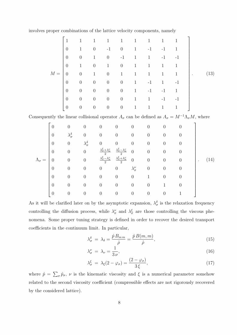
coefficients. The numerical results are reported by matrix form in Figure 6 and 7 for Sc∗1 and

Sc∗2 respectively. Every time that the numerical error is lower than 10 %, the correspoding

combination of trasport coefficients is marked as acceptable for the scheme. This constraint,

when applied to Sc∗2 is more restrictive than when applied to Sc∗1. This confirms that

taking into account different molecular weights by ϕσ < 1 may show some limits, in case

of large mass ratios. On the same plots, the theoretical values of the Schmidt numbers are

reported by some proper iso-values in the ranges Sc1 ∈ [4.3, 2880.6] and Sc2 ∈ [5.5, 3643.7]

respectively. In order to ensure the desired accuracy for both the transport coefficients for

any combination, the Schmidt numbers must be quite large: for this particular application,

they should be roughly larger than 1000.

Clearly from the numerical point of view, the separation of the characteristic scales,

which was assumed in the development of the scheme, works only asymptotically and the

stability/accuracy issues may reduce the actual applicability of scheme to a constrained

range of theoretical transport coefficients, depending on the considered application. By the

way, this situation is common to most of lattice Boltzmann schemes.

IV. CONCLUSIONS

A new LBM scheme for homogeneous mixture modeling, based on the multiple–

relaxation–time (MRT) formulation, which fully recovers Maxwell–Stefan diffusion model

in the continuum limit with (a) external force and (b) tunable Schmidt number, was de-

veloped. This formulation allows one to tune the relaxation frequencies of the collisional

matrix independently each other, and, in particular for the present application, it allows one

to tune the mixture kinematic viscosity independently on the Maxwell–Stefan diffusion resis-

tances. This is part of an on-going effort to improve existing LBM scheme for homogeneous

mixtures. The same author already proposed a new scheme based on the theoretical basis

of a recently proposed BGK-type kinetic model for gas mixtures [21], which used only one

relaxation parameter. The actual MRT formulation substantially extended the applicability

of the previous model.

The numerical simulations for the solvent test case with external force, confirmed the

23

validity of the proposed formulation and they allowed us to find out the numerical ranges

for the transport coefficients, which ensure acceptable accuracies. The numerical results

prove a contraction of the theoretical expectations, which were based on a strong separation

among the characteristic scales. Essentially the Schmidt number needs to be large enough

to ensure acceptable results.

Acknowledgments

The author would like to thank prof. Li-Shi Luo of Old Dominion University (USA) and

prof. Taku Ohwada of Kyoto University (Japan) for many enlightening discussions con-

cerning the kinetic equations for mixtures and the asymptotic analysis of kinetic equations

respectively. Moreover he would like to thank dr. Ilya Karlin of ETH-Zurich (Switzerland)

for pointing out the new results reported in Ref. [16] and Lin Zheng of Huazhong University

of Science and Technology (China) for pointing out how to select λδσ in such a way that χσς

is symmetric.

[1] G. R. McNamara and G. Zanetti, Phys. Rev. Lett. 61, 2332 (1988).

[2] F. J. Higuera and J. Jimenez, Europhys. Lett. 9, 663 (1989).

[3] F. J. Higuera, S. Succi, and R. Benzi, Europhys. Lett. 9, 345 (1989).

[4] H. Chen, S. Chen, and W. Matthaeus, Phys. Rev. A 45, R5339 (1992).

[5] Y. Qian, D. d’Humieres, and P. Lallemand, Europhys. Lett. 17, 479 (1992).

[6] X. He and L.-S. Luo, Phys. Rev. E 55, R6333 (1997).

[7] X. Shan and X. He, Phys. Rev. Lett. 80, 65 (1998).

[8] M. Ancona, J. Computat. Phys. 115, 107 (1994).

[9] M. Junk, Numer. Methods Part. Diff. Eq. 17, 383 (2001).

[10] R. Benzi, S. Succi, and M. Vergassola, Phys. Rep. 222, 145 (1992).

[11] S. Chen and G. D. Doolen, Annu. Rev. Fluid Mech. 30, 329 (1998).

[12] G. D. Doolen (Editor), ed., Lattice Gas Methods for Partial Differential Equations (Addison-

Wesley, New York, 1990).

[13] D. Wolf-Gladrow, Lattice-Gas Cellular Automata and Lattice Boltzmann Models, no. 1725 in

24

Lecture Notes in Mathematics (Springer-Verlag, Berlin, 2000), 2nd ed.

[14] S. Succi, The Lattice Boltzmann Equation for Fluid Dynamics and Beyond (Oxford University

Press, New York, 2001), 2nd ed.

[15] P. Asinari (2008), submitted to Phys. Rev. E.

[16] S. Arcidiacono, I. V. Karlin, J. Mantzaras, and C. E. Frouzakis, Phys. Rev. E 76, 046703

(2007).

[17] B. B. Hamel, Phys. Fluids 8, 418 (1965).

[18] B. B. Hamel, Phys. Fluids 9, 12 (1966).

[19] F. Williams, Combustion Theory (Benjamin/Cumming, California, 1986).

[20] V. Garzo, A. dos Santos, and J. J. Brey, Phys. Fluids A 1, 380 (1989).

[21] P. Andries, K. Aoki, and B. Perthame, J. Stat. Phys. 106, 993 (2002).

[22] J. C. Maxwell, Philos. Trans. R. Soc. 157, 26 (1866).

[23] E. P. Gross and M. Krook, Phys. Rev. 102, 593 (1956).

[24] P. L. Bhatnagar, E. P. Gross, and M. Krook, Phys. Rev. 94, 511 (1954).

[25] P. Asinari, Phys. Rev. E 73, 056705 (2006).

[26] M. E. McCracken and J. Abraham, Phys. Rev. E 71, 046704 (2005).

[27] D. d’Humieres, in Rarefied Gas Dynamics: Theory and Simulations, edited by B. D. Shizgal

and D. P. Weave (AIAA, Washington, D.C., 1992), vol. 159 of Prog. Astronaut. Aeronaut.,

pp. 450–458.

[28] P. Lallemand and L.-S. Luo, Phys. Rev. E 61, 6546 (2000).

[29] D. d’Humieres, I. Ginzburg, M. Krafczyk, P. Lallemand, and L.-S. Luo, Philos. Trans. R. Soc.

Lond. A 360, 437 (2002).

[30] P. Asinari, Phys. Fluids 17, 067102 (2005).

[31] M. Junk, A. Klar, and L.-S. Luo, J. Computat. Phys. 210, 676 (2005).

[32] Y. Sone, Kinetic Theory and Fluid Dynamics (Birkhauser, Boston, 2002), 2nd ed.

[33] H. Struchtrup, Macroscopic Transport Equations for Rarefied Gas Flows – Approximation

Methods in Kinetic Theory, Interaction ofMechanics andMathematics Series (Springer, Hei-

delberg, 2005).

[34] P. Asinari and T. Ohwada (2008), submitted to Comput. Math. Appl.

[35] H. Struchtrup, J. Stat. Phys. 125, 565 (2006).

[36] H. Struchtrup, Phys. Fluids 16, 3921 (2004).

25

[37] H. Struchtrup, Multiscale Model. Simul. 3, 211 (2004).

[38] Z. L. Guo and T. S. Zhao, Phys. Rev. E 67, 066709 (2003).

[39] A. Bardow, I. Karlin, and A. Gusev, Europhys. Lett. 75, 434 (2006).

[40] W. S. R.B. Bird and E. Lightfoot, Transport Phenomena (John Wiley & Sons, New York,

1960).

[41] C. Brennen, Fundamentals of Multiphase Flow (Cambridge University Press, United Kingdom,

2005).

[42] E. G. Flekkoy, Phys. Rev. E 47, 4247 (1993).

[43] I. Ginzburg and D. d’Humieres, Phys. Rev. E 68, 066614 (2003).

[44] M. Junk and Z. Yang, J. Stat. Phys. 121, 3 (2005).

26

FIG. 1: Iso-contours of the molar concentration y1 in the domain [0, L1]× [0, L2] at the time step

t = T = 600 δt, for the solvent test case of a ternary mixture (y3∼= 1 and consequently y1

∼= 0 and

y2∼= 0).

27

FIG. 2: Iso-contours of the molar concentration y2 in the domain [0, L1]× [0, L2] at the time step

t = T = 600 δt, for the solvent test case of a ternary mixture (y3∼= 1 and consequently y1

∼= 0 and

y2∼= 0).

28

FIG. 3: Solvent test case for a ternary mixture: y3∼= 1 and consequently y1

∼= 0 and y2∼= 0.

Comparison between theoretical kinematic viscosity ν ∈ [1, 20] and the numerical viscosity ν∗ of

the proposed scheme, measured by Eq. (60), for different values of the Maxwell–Stefan coefficients.

29

FIG. 4: Solvent test case for a ternary mixture: y3∼= 1 and consequently y1

∼= 0 and y2∼= 0.

Comparison between theoretical Maxwell–Stefan resistance coefficient for component 1, i.e. B13,

with the numerical resistance coefficient B∗13 of the proposed scheme, measured by Eq. (64), for

different values of the kinematic viscosity.

30

FIG. 5: Solvent test case for a ternary mixture: y3∼= 1 and consequently y1

∼= 0 and y2∼= 0.

Comparison between theoretical Maxwell–Stefan resistance coefficient for component 2, i.e. B23,

with the numerical resistance coefficient B∗23 of the proposed scheme, measured by Eq. (65), for

different values of the kinematic viscosity.

31

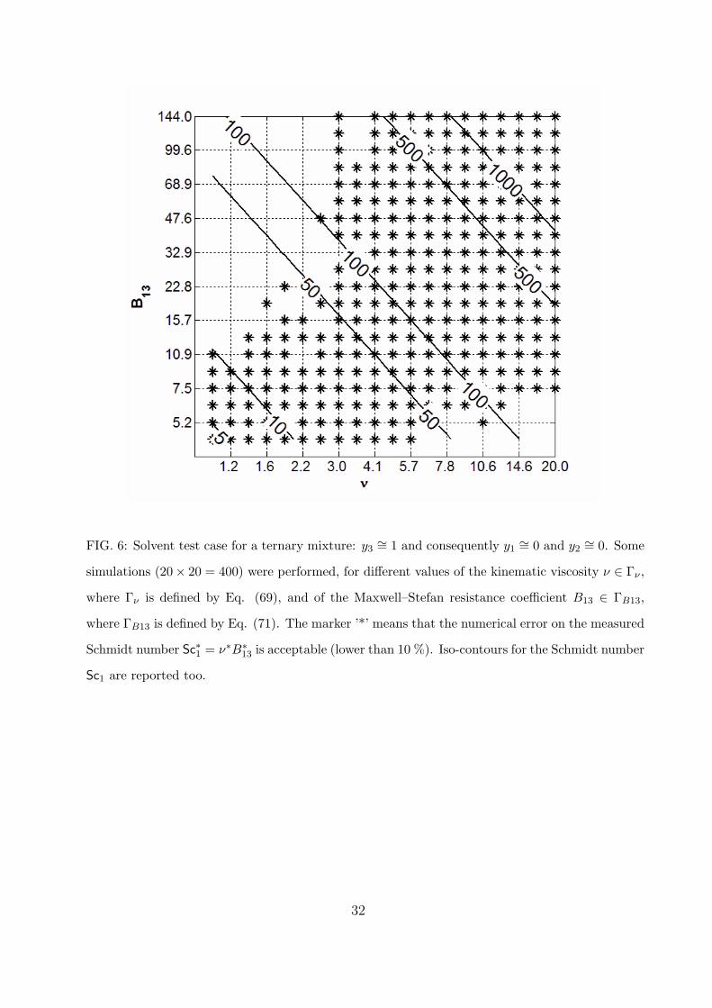
FIG. 6: Solvent test case for a ternary mixture: y3∼= 1 and consequently y1

∼= 0 and y2∼= 0. Some

simulations (20× 20 = 400) were performed, for different values of the kinematic viscosity ν ∈ Γν ,

where Γν is defined by Eq. (69), and of the Maxwell–Stefan resistance coefficient B13 ∈ ΓB13,

where ΓB13 is defined by Eq. (71). The marker ’*’ means that the numerical error on the measured

Schmidt number Sc∗1 = ν∗B∗13 is acceptable (lower than 10 %). Iso-contours for the Schmidt number

Sc1 are reported too.

32

FIG. 7: Solvent test case for a ternary mixture: y3∼= 1 and consequently y1

∼= 0 and y2∼= 0. Some

simulations (20× 20 = 400) were performed, for different values of the kinematic viscosity ν ∈ Γν ,

where Γν is defined by Eq. (69), and of the Maxwell–Stefan resistance coefficient B23 ∈ ΓB23,

where ΓB23 is defined by Eq. (72). The marker ’*’ means that the numerical error on the measured

Schmidt number Sc∗2 = ν∗B∗23 is acceptable (lower than 10 %). Iso-contours for the Schmidt number

Sc2 are reported too.

33