Multiple Step Financial Time Series Prediction with...
85
MULTIPLE STEP FINANCIAL TIME SERIES PREDICTION WITH PORTFOLIO OPTIMIZATION by David Hugo Diggs A THESIS SUBMITTED TO THE FACULTY OF THE GRADUATE SCHOOL MARQUETTE UNIVERSITY IN PARTIAL FULFILLMENT OF THE REQUIREMENTS for the degree of MASTER OF SCIENCE in Electrical and Computer Engineering Milwaukee, Wisconsin June 2004
Transcript of Multiple Step Financial Time Series Prediction with...

MULTIPLE STEP FINANCIAL TIME SERIES PREDICTION WITH
PORTFOLIO OPTIMIZATION
by
David Hugo Diggs
A THESIS SUBMITTED TO THE
FACULTY OF THE GRADUATE SCHOOL
MARQUETTE UNIVERSITY
IN PARTIAL FULFILLMENT OF THE REQUIREMENTS
for the degree of
MASTER OF SCIENCE
in Electrical and Computer Engineering
Milwaukee, Wisconsin
June 2004

ii
Acknowledgement
First and foremost, I would like to thank God, for without him none of this would
be possible. Next I would like to thank my family, especially my mom, dad, and
grandmother for all of their love a support throughout my life. I would also like to extend
a thank you to all of my friends at home, at Marquette, and in the KID lab. I greatly
appreciate the help I received from my committee members on this thesis and in class.
Last but not even close to least, I would like to extend a special thanks to Dr. Povinelli
being a role model on how to succeed in academics and for giving me a new perspective
on how to value family life.

iii
Abstract
The Time Series Data Mining framework developed by Povinelli is extended to
perform weekly multiple time-step prediction and adapted to perform weekly stock
selection from a broader market. The stock selections are combined into weekly
portfolios, and techniques from Modern Portfolio Theory and the Capital Asset Pricing
Model are adapted to optimize the portfolios. The contribution of this work is the
combination of stock selection and portfolio optimization to develop a temporal data
mining based stock trading strategy. Results show that investors can increase overall
wealth, obtain optimal weekly portfolios that maximize return for a given level of
portfolio risk, overcome trading costs associated with trading on a weekly basis, and
outperform the market over a given time range.

iv
Table of Contents
Chapter 1 Introduction………………………………………………………………...1
1.1 Motivation/Goal……………………………………………………………….1
1.2 Problem Statement…………………………………………………………….2
1.3 Thesis Outline…………………………………………………………………3 Chapter 2 Background………………………………………………………………...5
2.1 Temporal Data Mining Overview……………………………………………..5 2.2 Reconstructed Phase Space……………………………………………………6 2.3 Genetic Algorithm…………………………………………………………….9
2.4 Time Series Data Mining.…………………………………………………....13
2.4.1 Concepts and Definitions………………………………………………14
2.4.2 Time Series Data Mining Method……………………………………...20 2.5 Portfolio Background………………………………………………………...25
2.6 Portfolio Optimization……………………………………………………….26
2.6.1 Modern Portfolio Theory………………………………………………27 2.6.2 Capital Asset Pricing Model…………………………………………...32 Chapter 3 Methods…………………………………………………………………...36
3.1 Stock Selection Method……………………………………………………...37
3.2 Modified Portfolio Optimization Method……………………………………39
3.3 Time Series Data Mining Portfolio Optimization Trading Strategy…………41
Chapter 4 Evaluation…………………………………………………………………44
4.1 Stock Market Application……………………………………………………44 4.2 Transaction Cost Model……………………………………………………...45

v
4.3 Experiments………………………………………………………………….46
4.4 Results………………………………………………………………………..48
4.4.1 Portfolio Return………………………………………………………..48
4.4.2 Portfolio Risk…………………………………………………………..61
4.4.3 Prediction Accuracy……………………………………………………63
Chapter 5 Conclusions and Future Work………………………………………...67 5.1 Research Conclusions…………………………………………………...67 5.2 Future Work………………………………………………………….….69
References ……………………………………………………………………….71
Appendix………………………………………………………………..………..76

vi
Table of Figures Figure 2.1: Example Time Series…………………………………...……………………..8
Figure 2.2: Example Reconstructed Phase Space…………………..……………………..8
Figure 2.3: Chromosome Crossover…………………..…………………………………11
Figure 2.4: Genetic Algorithm Process…………………………………………………..12
Figure 2.5: Diagram of Time Series Data Mining Method…………………..………..…14
Figure 2.6: GM Stock Price Time Series………………………………………..…….…15
Figure 2.7: GM Daily Percent Change…………………………………………………..17
Figure 2.8: Reconstructed Phase Space………………………………………………….18
Figure 2.9: Augmented Phase Space…………………………………………………….19
Figure 2.10: Multi-Step Prediction……………………………………………………....23
Figure 2.11: Efficient Frontier…………………………………………………………...31
Figure 2.12: Capital Market Line………………………………………………………...34
Figure 3.1: Time Series Data Mining Portfolio Optimization Method…………………..37
Figure 3.2: Time Series Data Mining Stock Selection Method..……………..……..…...38
Figure 3.3: Model Market Portfolio……………………………………………………...41
Figure 4.1: 2002 Dow Jones 30 Portfolio Rate of Return One-step prediction………….52
Figure 4.2: 2002 Dow Jones 30 Portfolio Rate of Return Two-step prediction…………53
Figure 4.3: 2002 Dow Jones 30 Portfolio Rate of Return Three-step prediction………..54
Figure 4.4: 2002 Dow Jones 30 Portfolio Rate of Return Four-step prediction…………55
Figure 4.5: 2003 Dow Jones 30 Portfolio Rate of Return One-step prediction………….56
Figure 4.6: 2003 Dow Jones 30 Portfolio Rate of Return Two-step prediction…………57
Figure 4.7: 2003 Dow Jones 30 Portfolio Rate of Return Three-step prediction………..58

vii
Figure 4.8: 2003 Dow Jones 30 Portfolio Rate of Return Four-step prediction…………59
Figure 4.9: Observed Optimal Portfolio w/Efficient Frontier…………………………...61

viii
Table of Tables Table 2.1: Chromosome Example………………………………..……………………...10
Table 2.2: Crossover Process Example……………………………………………..…...11
Table 2.3: Mutation Example…………………………………………………………....11
Table 2.4: Phase Space Points…………………………………………………………...18
Table 4.1: Dow Jones 30 Return Performance 1/01/2002 –1/01/2003…………………..49
Table 4.2: Dow Jones 30 Return Performance 1/01/2003 –1/01/2004…………………..50
Table 4.3: Dow Jones 30 Risk Analysis 1/01/2002 – 1/01/2003………………………...63
Table 4.4: Dow Jones 30 Risk Analysis 1/01/2003 – 1/01/2004………………………...63
Table 4.5: Prediction Accuracy Analysis 1/01/2002 – 1/01/2003……………………….65
Table 4.6: Prediction Accuracy Analysis 1/01/2003 – 1/01/2004……………………….66

Chapter 1 Introduction 1
Chapter 1 Introduction 1.1 Motivation
The financial markets are perennially attractive to researchers from a wide range of
fields [1, 2]. This attraction is due to the lure of easy money, if only a method to perfectly
predict the dynamics of the market could be discovered. From a more scientific stance,
the financial markets are interesting because of their incredible complexity and time
varying dynamics. The interests of millions of investors are represented through the rise
and fall of stocks prices and the companies they represent.
The dynamics of the stock market have been modeled in many ways. Box and Jenkins
showed that the ARIMA model was a good first approximation [3, 4]. This model can be
understood as a random walk process. Further financial research has produced more
robust versions of the random walk model including the efficient market hypothesis [5].
All of these models of the market assume that all information is represented in the market
immediately and that any attempt to profit through arbitrage will fail, because the stocks
are correctly valued.
However, despite this theory, there is a never-ending attempt by technicians to model
the stock market dynamics to achieve superior returns [6, 7]. Examples of statistical
trading strategies include chart analysis, momentum or swing trading, and trend trading
[1, 6-8]. Each of theses strategies attempts to outperform market benchmarks by
providing above market returns without significantly increasing risk.
Recently, stock market research has become more attractive because of the increased
access to financial data and the ability to invest independently. Websites such as
http://finance.yahoo.com, http://esignal.com, and http://moneycentral.msn.com give

Chapter 1 Introduction 2
investors access to current and reliable financial information along with overall market
conditions for investing. Online trading sites such as TDWaterhouse.com, Etrade.com,
and Ameritrade.com, have allowed small investors to easily set up and manage their own
investments. This combination of reliable financial data access and easy online trading is
important in developing and testing an investment strategy.
The work presented in this thesis is in the nature of a technical approach. We
attempt to identify hidden patterns in the market data that are predictive of increases in a
stock price. The unique nature of this work is the combination of dynamical systems
theory with portfolio optimization techniques and the study of this approach across
different prediction horizons and market conditions [9].
1.2 Problem Statement
The goal of this research is to create a profitable trading strategy that overcomes
transaction cost and outperforms the overall market returns. The proposed trading
strategy combines stock selection, asset allocation, and risk management techniques.
Stock selection is the process of identifying assets that have desired characteristics, and
asset allocation is the process of weighting individual assets to build a portfolio. Risk
management is the process of identifying and minimizing the impact of uncertain events.
Asset allocation and risk management can be used to reduce risk by diversifying a
portfolio. Portfolio optimization is the integration of asset allocation and risk
management to create portfolios that meet specific risk and return criteria.
In this research, stock selection is accomplished using a nonlinear time series
prediction approach [3]. The approach seeks to discover hidden structures in
reconstructed phase spaces of the stock price time series to make predictions on future

Chapter 1 Introduction 3
stock price movements. The details of reconstructed phase spaces and the data mining
approach for stock selection are found in Chapter 2.
Once stock selection is completed, optimal portfolios are constructed using
techniques based on Modern Portfolio Theory and the Capital Asset Pricing Model [2, 7].
Modern Portfolio Theory, developed by Harry Markowitz, makes the assumption that
investors differ only in their expectations of return required for a particular investment
and risk tolerance. Modern Portfolio Theory provides the techniques to create a set of
portfolios that are optimal in the sense that they maximize portfolio return for a given
level of portfolio risk [2, 5, 9]. The Capital Asset Model extends Modern Portfolio
Theory by determining a method for selecting a specific optimal portfolio from a set of
optimal portfolios.
This research contributes a trading strategy that employs a temporal data mining
approach to stock selection combined with portfolio optimization. The trading strategy
trades periodic weekly portfolios, by buying the entire portfolio at the beginning of the
period and selling it at the end of the period.
1.3 Thesis Outline
This thesis consists of five chapters. Chapter 2 reviews the Time Series Data
Mining Method (TSDM), the stock selection approach used here, and traditional portfolio
optimization techniques. Chapter 3 describes the problem-specific methods used in stock
selection and portfolio optimization. It also presents the extensions and adaptations of the
TSDM method along with the adapted portfolio optimization techniques used to develop
the proposed trading strategy. Chapter 4 evaluates the proposed methods on historical
data. This chapter details the stock market data sets, performance calculations, and

Chapter 1 Introduction 4
experimental results. Chapter 5 discusses the research results, conclusions, and
suggestions for future directions.

Chapter 2 Background 5
Chapter 2 Background
The Time Series Data Mining (TSDM) framework transforms market time series
into reconstructed phase spaces (RPSs) and searches these phase spaces for temporal
structures predictive of the greatest changes in the market time series [3]. This framework
combined with portfolio optimization, which involves modifying the weights of the assets
in a portfolio to achieve a specific investor goal or set of goals, is used to formulate a
portfolio trading strategy. The portfolio optimization techniques used here are based on
Modern Portfolio Theory (MPT) and the Capital Asset Pricing Model (CAPM) [1, 5].
The chapter presents an overview of the components used in developing the proposed
trading strategy.
2.1 Temporal Data Mining Overview
A time series is an ordered sequence of real-valued elements denoted by
, 1,..., ,nx x n N= = (2.1)
where n is the current time index, and N is the number of observations. Time series
appear in many forms in a variety of fields. Domains such as medicine, speech, and
finance have applications that involve the study of temporal data [10-14]. This thesis
applies temporal data mining techniques in the area of financial time series prediction.
Temporal data mining is a sub-field of data mining that focuses primarily on
discovering relationships between sequences of real valued time series events.
Techniques common to data mining and temporal data mining are association rule
learning, classification, clustering, and prediction [15-18]. The main difference between
temporal data mining and data mining in general is in how the data is represented. Often
time series signals are noisy, non-linear, and chaotic, making patterns and data

Chapter 2 Background 6
relationships hard to detect [19]. Linear and nonlinear time series transforms such as
linear filters and time series embedding techniques are used to modify the representation
of time series data without losing valuable information about the time series. Specific
time series transformation techniques such as the Discrete Fourier Transform, which
transforms a signal from the time domain into the frequency domain, and the Discrete
Wavelet Transform, which translates a time series into the time-frequency domain, have
been used to represent data in formats suitable for data mining tasks [20].
The TSDM approach has its foundation in temporal data mining using techniques
from machine learning, artificial intelligence, and genetic algorithms. The approach uses
a time-delay embedding technique called phase space reconstruction that creates a time-
lagged version of the original signal [3, 10]. The next section presents the concept and
theoretical definition of a reconstructed phase space.
2.2 Reconstructed Phase Space
This section discusses the definition of a reconstructed phase space and the
theoretical justification for using the technique in this thesis. The reconstructed phase
space is a time-delay embedding of an original time series and has been shown to capture
nonlinear information found in complex dynamical systems that have many dimensions
[3, 10, 21]. This technique creates a time-lagged version of a signal used to discover
hidden patterns normally not detected in a linear space. This approach provides the basis
for the data mining-based stock selection process presented later in this thesis.
A reconstructed phase space (RPS) is a d-dimensional metric space in which a
time series is unfolded. Takens proved that if the dimension of the embedding space is
large enough, then the RPS is topologically equivalent to the original state space that

Chapter 2 Background 7
generated the time series [20, 22, 23]. The RPS can be formed using a time delay
embedding process, which performs a homeomorphic mapping from one topological
space to another. The embedding process creates the RPS signal, which is a time-delayed
version of the original time series signal [19, 20, 23]. It maps a set of d time series
observations taken from a time series x on to
( ) ( )( )1 1 1n n nn dx x x n dττ τ−− − = = + x …N− , (2.2)
which is a vector or point in the phase space. Together the phase space points form a
trajectory matrix
( )
( )
( )
( )
( ) ( )( )
1 1 1 11 1
2 2 2 12 1
1 1
,
dd
dd
N d NN dN N d d
x x x
x x x
x x x
τ ττ
τ ττ
ττ τ
+ + −+ −
+ + −+ −
−− − − − ×
= =
x
xX
x
(2.3)
where d is the embedding dimension, τ is the time-lag, and nx is the signal value at time
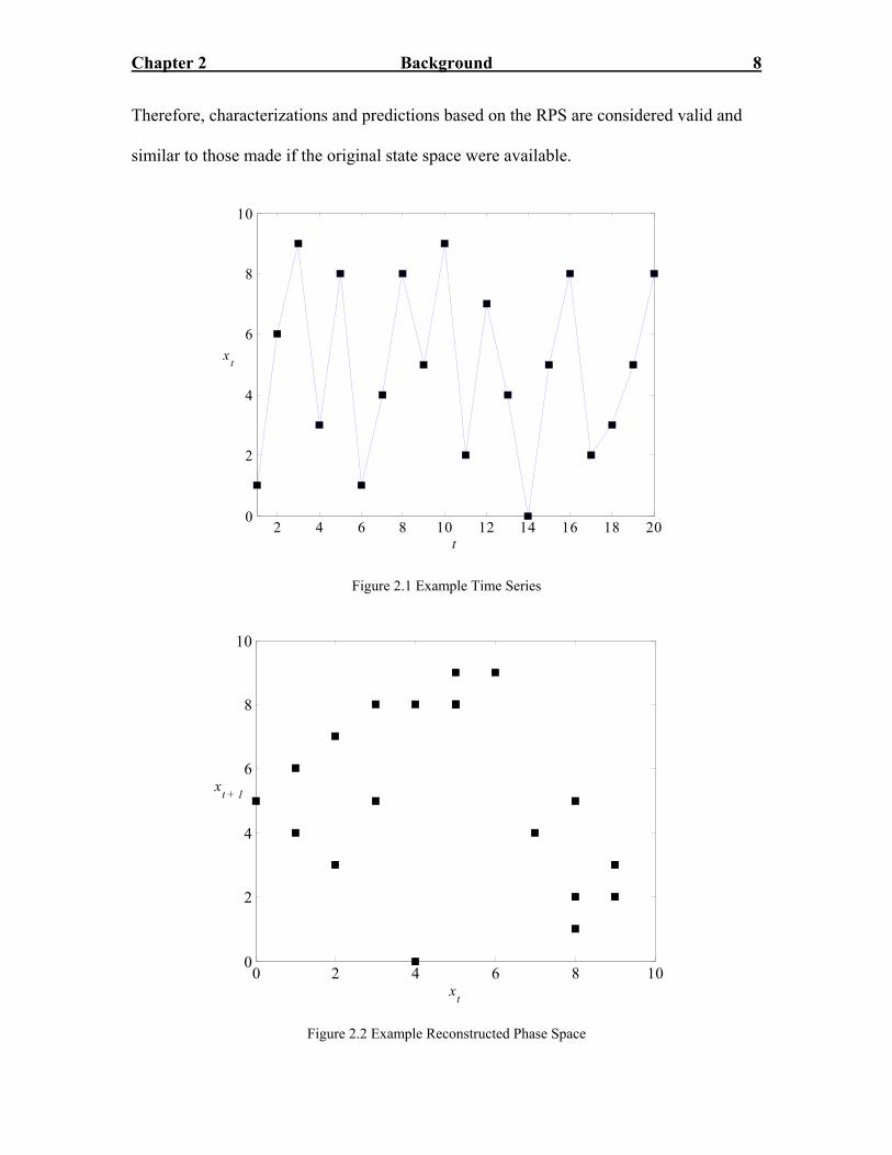
index n. Figure 2.2 shows an example of a RPS (a plot of the trajectory matrix) from a
randomly generated time series shown in Figure 2.1. The original time series is time-
delay embedded with a dimension of two to create the RPS. Equation 2.4 shows the first
five points in the trajectory matrix from Figure 2.2.
1 66 99 33 88 1
=
X (2.4)
Takens proved that if an embedding of a time series is performed correctly, then
the dynamics of the RPS are topologically equivalent to the original state space and the
RPS contains the same topological information as the original state space of system [21].
Chapter 2 Background 8
Therefore, characterizations and predictions based on the RPS are considered valid and
similar to those made if the original state space were available.
2 4 6 8 10 12 14 16 18 200
2
4
6
8
10
xt
t
Figure 2.1 Example Time Series
0 2 4 6 8 100
2
4
6
8
10
xt
xt + 1
Figure 2.2 Example Reconstructed Phase Space

Chapter 2 Background 9
2.3 Genetic Algorithm
The Time Series Data mining method uses a simple genetic algorithm as an
optimization method to discover predictive hidden patterns, with high fitness values, in
the reconstructed phase space. A genetic algorithm is a method of problem solving and
global optimization that uses computational models of evolutionary processes as elements
in design and implementation [24]. Genetic algorithms incorporate aspects of natural
selection to maintain a population of structures that evolves according to rules of
selection, recombination, mutation, and survival of the fittest. The fitness or performance
of each individual in the population determines which individuals are more likely to be
selected for reproduction, while recombination and mutation modify those individuals,
yielding potentially superior ones. This process leads to fitter populations corresponding
to better solutions to various problems. Genetic algorithms have been shown useful in
finding optimal solutions in non-linear functions [24].
The main concepts of a binary genetic algorithm are fitness, objective function,
chromosome, population, and generation [24]. A chromosome is a binary encoding of the
independent variables of the objective function. The fitness of a chromosome is the
application of the objective function to a decoded chromosome. A population is a set of
chromosomes. A generation is one iteration of the genetic algorithm, which is comprised
of the application of a set of operators to the population. The most frequently used
operators in genetic algorithms are selection, crossover, mutation, and reinsertion [24].
An objective function defines a rule for the search space where the optimizer is to
be found. A simple example of an objective function might be:
2( ) 100f x x x= + + . (2.5)

Chapter 2 Background 10
An example of a small population for a particular generation is shown in Table
2.1 with associated fitness values and chromosome lengths of eight.
Chromosome x f(x), fitness 00000000 0 100
01111111 127 16356
11111100 -4 112
Table 2.1 Chromosome Example
The first operator in a iteration of a genetic algorithm is typically selection. It is
the process of choosing chromosomes from a population based on each chromosome’s
fitness. The type of selection used in this work is roulette wheel selection in which a
chromosome is given a section of the roulette wheel based on the size of its fitness value.
The wheel is spun once, and the winning chromosome is selected for further
permutations.
The next typical operator is crossover, which is the process of combining
chromosomes in a manner similar to sexual reproduction. The crossover operator
combines segments from the encoded format of each parent to create offspring
chromosomes shown in Figure 2.3. Crossover can be accomplished using either a fixed or
a random crossover locus.

Chapter 2 Background 11
crossover locus crossover locus
1head 1tail
2head 2tail
1head
2tail
1tail
2head
crossover locus
1head
2head
2tail
1tail
Figure 2.3 Chromosome Crossover
An example of the crossover process is again showed in Table 2.2 with example
chromosomes.
Mating pair Parent 1 Parent 2 Offspring 1 Offspring 2 1 1111↑1100 0000↑0000 0000↑1100 1111↑0000
2 0000↑0000 1010↑1111 0000↑1111 1010↑0000
Table 2.2 Crossover Process Example
The mutation operator randomly changes the bits of the chromosomes as shown in
Table 2.3. The mutation operator is usually set at a specific mutation rate is used to
control an aspect of population evolution and periodically randomize the population to
avoid local minimums and maximums.
Pre-mutation Post-mutation 00001111 00011111
01010011 01011011
Table 2.3 Mutation Example
Reinsertion is the process of selecting only a small percentage of chromosomes to
bypass the operations of selection, crossover, and mutation. This technique allows the

Chapter 2 Background 12
individuals with the highest fitness to pass directly to the next generation without being
modified and ensures that elite individuals are not lost due to the stochastic nature of
selection and crossover. A genetic algorithm uses these steps, shown in Figure 2.4, to find
objective function optimizers.
Generate initial population of
solutions
Evaluation
Selection
Generate variant populations using mutation and crossover
Halting Criteria Met?
Mutation
Crossover
Reinsertion
End Yes
Figure 2.4 Genetic Algorithm Process
The simple genetic algorithm described above performs a se
phase space, generating subsequent chromosome population
met and a highly predictive temporal structure is found. The
algorithm process are:
No
arch in the reconstructed
s until a stopping criterion is
steps in the simple genetic

Chapter 2 Background 13
• Random population initialization
• Calculate fitness
• While fitness value have not converged
o Selection
o Crossover
o Mutation
o Reinsertion
2.4 Time Series Data Mining
Time Series Data Mining employs a time-delay embedding process that embeds a
time series into a reconstructed phase space (RPS), shown in Figures 2.1 and 2.2. The
RPS, discussed in Section 2.2, is topologically equivalent to the original system that
generated the time series [22, 23]. The TSDM method also uses a genetic algorithm
search, discussed in Section 2.3, to discover hidden temporal structures in a time-delay
embedded signal that are characteristic and predictive of time series events, where
temporal structures are a predictive sequence of points found in time series data that
signal future outcomes and events. The temporal structures found in the time series data
are used to predict sharp movements in a time series. Originally, the TSDM technique
was applied to making one-step time series predictions such as predicting sharp increase
in daily stock price or welding droplet release times [10, 25, 26]. Here it is applied to
make predictions on a weekly basis [27].
To better explain the TSDM method, we introduce a set of concepts. The concepts
are opportunities, events, goal function, temporal pattern, temporal structure,
reconstructed phase space, augmented phase space, average event function, and ranking

Chapter 2 Background 14
function. Figure 2.5 shows how the concepts relate to the overall Time Series Data
Mining method. As with machine learning approaches, the method is composed of a
training stage and a testing stage. The training stage defines the prediction goal and
identifies predictive structures in training signal of the embedded time series data. The
testing stage uses the predictive temporal structure found during training to predict
events.
Define goal function, ranking function and
optimization formulation
Select embedding dimension
Search phase space for predictive temporal
structures
Embed testing period time series
Predict events using selected temporal
Observed time series
Testing Stage
Training Stage
Embed training period time series
Figure 2.5 Diagram of Time Series Data Mining Method
2.4.1 Concepts and Definitions Time Series Data Mining method concepts are defined and explained with
examples for each concept. Each concept refers to a step in the TSDM method and
defines the actions taken in each step.
Events are defined as important occurrences in time. Opportunities are defined as
chances to take advantage of significant events that occur over time. Events and

Chapter 2 Background 15
opportunities are discovered in time series data such as a stock price time series shown
as,
1,..., ,nx x n N= = (2.5)
which represent the price movements of a stock over a time period with length N and
price nx . An important occurrence in the stock price time series is an increase in the stock
price. For example, the rise in a stock price, over a given period, represents an
opportunity to take action by having purchased the stock before the start of that time
period. Figure 2.6 shows the daily stock time price time series for General Motors (GM)
from 1/01/2004 to 2/01/2004.
2 4 6 8 10 12 14 16 18 2036
36.5
37
37.5
38
38.5
39
39.5
40
40.5
Day
Stoc
k Pr
ice(
$)
Figure 2.6 GM Stock Price Time Series 1/01/2004 –2/01/2004
A prediction is defined as the expectation of the future price for a stock. Predictions are
labeled to determine the value and assessment of the prediction. A goal function g,

Chapter 2 Background 16
associates a future value to predictions made at the current time index n. The goal
function provides a mapping between the temporal structures found and the events
predicted. For example, a goal function can be the one period percent change in a stock
price at time index n given as,
+1.
( n nn
n
)x xgx−
= (2.6)
A temporal pattern tp is a hidden pattern in a time series that is characteristic and
predictive of occurrences. A temporal pattern, Dtp ∈ , is defined as a vector of length D
or equivalently as a point in a D-dimensional real metric space.
A temporal structure TS is defined as the surrounding set of all points within δ of
the temporal pattern shown as,
{ : ( , )DTS a d tp a },δ= ∈ ≤ (2.7)
where d is the Euclidean distance metric defining a hyper-sphere with center tp and
radius δ. Figure 2.7 shows an example of a temporal structure used to predict an event
with the associated prediction value.

Chapter 2 Background 17
2 4 6 8 10 12 14 16 18 20
-0.04
-0.03
-0.02
-0.01
0
0.01
0.02
0.03
Figure 2.7 GM Daily Percent Change 1/01/2004 – 2/01/2004
Day
Perc
ent C
hang
ePredicted Event
Three Point Predictive Structure
A reconstructed phase space (RPS) is a d-dimensional real metric space into
which the time series is embedded as shown in Section 2.2. The reconstructed phase
space signal is a time-lagged version of the original time series signal [19, 20]. Figure
2.8 shows General Motors’ percent change time series reconstructed into the phase space.
Table 2.4 highlights the numerical mapping of the first five points in General Motors’
percent change time series to equivalent points in the phase space with an embedding
dimension of 2.

Chapter 2 Background 18
-0.05 -0.04 -0.03 -0.02 -0.01 0 0.01 0.02 0.03 0.04-0.05
-0.04
-0.03
-0.02
-0.01
0
0.01
0.02
0.03
0.04
xt
xt + 1
Figure 2.8 Reconstructed Phase Space
Original Time Series ( , )t tx y Coordinates
Reconstructed Phase Space 1( , )t tx x + Coordinates
(02-Jan-2003, 0.000) (0.000, -0.0105) (03-Jan-2003, -0.0105) (-0.0105, 0.0246) (06-Jan-2003, 0.0246) (0.0246, 0.0089) (07-Jan-2003, 0.0089) (0.0089, -0.0409)
(08-Jan-2003, -0.0409) (-0.0409, 0.0338)
Table 2.4 Phase Space Points
The augmented phase space is a d+1 dimensional space formed by extending the
phase space with the additional dimension of . The augmented phase gives
visualization to the value of the temporal structures in the reconstructed phase. The
ng

Chapter 2 Background 19
augmented phase space illustrated in Figure 2.9 represents the extension from the
reconstructed phase space in Figure 2.8.
-0.06 -0.04 -0.02 0 0.02 0.04-0.05
0
0.05-0.05
0
0.05
xtxt - 1
g
Figure 2.9 Augmented Phase Space
The average event function Mµ represents a fitness value given to a temporal
structure, TS. This function maps a structure onto the real line to allow the temporal
structures to be ranked ordered. The average value Mµ , of the points that are within a
temporal structure is
1 ,( )M n
t Mg
c Mµ
∈
= ∑ (2.8)
where c M is the cardinality of M, the set of all points that are within a temporal
structure. In contrast, the average value
( )
Mµ of the points that are not within a temporal
structure is denoted as
1 ,( ) nM
t M
gc M
µ∈
= ∑ (2.9)

Chapter 2 Background 20
where c M is the cardinality of( ) M , the set of all points not within a temporal structure.
A ranking function f, shown in Equation 2.10, is used to show structures that
determine optimal temporal structures that characterize and predict events. The ranking
function,
( ) min min( )
if ( ) ( )( ) otherewise
Mc M
M c
c M cf TS g gβ
µ βµ
>= − + X
X, (2.10)
where β is a barrier function designed to ensure a minimum number of phase space points
are within each temporal structure, is the minimum prediction event value, and
is the cardinality of all phase space points. This particular ranking function allows
the TSDM method to make predictions that have high average percent change values [3,
28].
ming
( )c X
These concepts are combined in the following TSDM method. The main goal of
the TSDM method is to find temporal structure used for predicting events. The selected
temporal structure is the structure with the highest fitness value found during the training
period. A genetic algorithm-based optimization process, described within the TSDM
method, is used to search for predictive temporal structures.
2.4.2 Time Series Data Mining Method
The steps for the Time Series Data Mining Method are listed below. These steps
refer to diagram of the TSDM method in Figure 2.5 (shown below) and the concepts
defined in Section 2.4.1. The TSDM method diagram precedes the list, and an
explanation is then provided for each step in the list.

Chapter 2 Background 21
Define goal function, ranking function and
optimization formulation
Select embedding dimension
Search phase space for optimal temporal
structures
Embed testing period time series
Predict events using selected temporal
Observed time series
Testing Stage
Training Stage
Embed training period time series
Figure 2.5 Diagram of Time Series Data Mining Method
TSDM Method Steps
1. Define the event to be predicted.
2. Define the opportunity based on the predicted events.
3. Evaluate events with the goal function.
4. Embed training signal into a reconstructed phase space (RPS).
5. Locate temporal structures and evaluate with associated fitness values.
6. Determine predictive temporal structures in the training signal by defining a
ranking function and an optimization formulation.
7. Embed testing signal into RPS.
8. Make predictions in the testing signal using the selected temporal structure.
9. Shift the window one time-step ahead and repeat steps 1-8.

Chapter 2 Background 22
The first step in applying the TSDM method to a particular problem is defining a
TSDM goal. Given an observed time series, the goal is to find otherwise hidden temporal
structures that are predictive of events in the time series. The events to be predicted are
determined by the defined TSDM goal.
With a TSDM goal clearly defined, a given time series will be observed for
predictive structures, and predictions will be made using the time series data. The TSDM
method is composed of a training stage followed by a testing stage. Here, the time series,
for which predictions are being made, is separated into a training signal and testing
signal. The training signal is defined by a training period of t weeks, starting t weeks
before the current time index n. The testing signal,
{ , ,..., } nY x n B E N B E= = < < , (2.11)
in a time series nx , is defined by the current time index n from the beginning B, through
the end of the testing signal E, where N is the end of the training period signal. The
prediction point is located at length of t prediction steps away from the current time index
n. The method makes a t-step prediction, denoted by n ng x t+= , and uses a sliding
window, which slides one time-step ahead after the training and testing stages are
completed for the current time index n. The widow size is the length of the training signal
in addition to the value of the step-size n for the given prediction denoted,
{ , ,..., } .nW x n B E t N B E= = + < < (2.12)
An example of the multi-step prediction process is shown in Figure 2.10. It provides both
a one-step prediction and a two-step prediction. The prediction step size t is chosen
before experimentation.

Chapter 2 Background 23
2 4 6 8 10 12 14 16 18 20
-0.04
-0.03
-0.02
-0.01
0
0.01
0.02
0.03
Figure 2.10 Multi-Step Prediction
Date
Perc
ent C
hang
eTwo step
Prediction Event
One step Prediction Event
Predictive Structure
The training stage begins by determining the TSDM objective in terms of the
opportunity, event, and associated goal function . The given time series is time delay
embedded into a phase space, and an associated percent change event value is given to
each time-step in the phase space. From the RPS and the associated percent change
function, we form the augmented phase space. The training stage continues with the
location of temporal structures in the reconstructed phase space. Temporal pattern
structures are defined with the n previous time series data points. After being embedded
into a reconstructed phase space, each point in the phase space is a temporal pattern. The
sphere surrounding that current point in the phase space with a Euclidean distance δ is a
temporal pattern structure. These temporal structures are evaluated using the average of
all points that lie within the temporal structure.
ng

Chapter 2 Background 24
The TSDM method then defines an objective for determining the best temporal
structure. The TSDM objective includes defining the ranking function ( )f TS , shown in
Equation 2.8, and optimization formulation. The ranking function and the optimization
are defined to determine predictive temporal patterns found in the training stage. The
ranking function ( )f TS rank orders the temporal structures, according to their fitness
values, found during the testing stage.
The temporal structure is determined by performing a search using a simple
genetic algorithm (sGA). The sGA obtains maximum fitness values by finding the
parameters that maximize the ranking function ( )f TS , denoted ,
max ( )tp
f TSδ
. The steps in
the genetic algorithm process are initialization followed by selection, fitness calculation,
crossover, mutation, and reinsertion, which are performed until a stopping criterion is
met. Monte Carlo search is used for random population initialization to determine the
number chromosomes in the genetic algorithm. The sGA performs roulette selection,
which probabilistically selects chromosomes based upon fitness value and random locus
crossover, which merges chromosomes in a manner similar to sexual reproduction, to
find predictive temporal structures [29-31]. The genetic algorithm evaluates fitness
values and continues searching until the minimum fitness values have converged to a
pre-specified convergence value. The chosen convergence value is used to halt
the genetic algorithm search when the ratio of the worst fitness value to the best
fitness value is equal to or above the convergence value. The results from the
training stage are examined and used to make predictions in the following testing stage.
During the testing stage of the method, a t-step prediction is made. For example if
t = 1, then a one-step prediction is made. The testing time series is embedded into the
phase space. The selected temporal structure from the training stage is used to predict

Chapter 2 Background 25
events at the current time index. If a sequence of embedded time series points from the
testing signal falls within the selected temporal structure, then a prediction is made. This
predicted event is evaluated using the appropriate goal function. The results of the testing
stage are evaluated, the time range window is shifted one time-step ahead, and the
process repeats starting with the training stage. The entire process of training and testing
continues, making predictions and evaluations for each time index n, until the end of the
time range T n . The following section presents portfolio background
material used to form a basis for portfolio optimization.
{ 1,..., }N= =
2.5 Portfolio Background
A portfolio is a set of stocks from the broader market that are combined and
weighted to become one investment [1, 5, 32]. Portfolios are evaluated on many criteria
such as return and risk. The return of a single asset in a portfolio is the gain or loss in that
asset’s value for a particular period, in percentage terms. The expected return is estimated
as the average of prior returns. Portfolio returns are the combined returns of all assets in a
portfolio with their associated weighting.
Risk is either the volatility of future outcomes or the probability of an adverse
outcome [2, 5]. There are two types of risk. The first is unsystematic risk or company
specific risk, which is unique to a company stock price time series. This type of risk can
be removed through diversification, which is a technique that combines a variety of
investments within a portfolio with the intention to minimize the impact of any one
security on overall portfolio performance [2]. The second is systematic or market risk,
which is variable risk caused by economic conditions [2]. Systematic risk cannot be
minimized through diversification because it is risk that all investors and companies incur

Chapter 2 Background 26
in the marketplace. Modern Portfolio Theory defines risk as the variance of expected
returns, whereas the Capital Asset Pricing Model defines risk relative to the overall
market.
Investors determine a risk vs. return trade off criterion, establishing how much
risk they are willing to take. Traditionally, low risk levels are associated with low
potential returns, and elevated risks levels are associated with higher potential returns.
This research assumes an investor is risk adverse and will only except higher risk levels
in return for a higher profit.
Diversification is a portfolio risk management technique that combines a large set
of investments within a portfolio. Diversification improves risk vs. return tradeoffs by
combining stocks with different risk and return characteristics from different sectors of
the overall market. The cross correlation and asset allocation among these assets allows
for alternate portfolios to be generated that have better risk vs. return characteristics than
any one asset by itself, thus becoming the main goal for portfolio optimization. In other
words, individual company risk or unsystematic risk can be minimized by properly
weighting the investments in a portfolio. The next sections present the concept of
portfolio optimization and the techniques used to perform it.
2.6 Portfolio Optimization
Portfolio optimization is the analysis and management of a portfolio to obtain the
maximum portfolio return for a given amount of portfolio risk. Activities such as asset
allocation, which divides the portfolio value among assets in the portfolio, and
diversification, allow an investor to meet specific investment goals or combination of
investment goals. Periodic evaluations of portfolio performance and modifications of the

Chapter 2 Background 27
weight values, also known as portfolio management, allows for various portfolio
combinations to meet various optimization criteria, such as maximizing return,
minimizing risk, and achieving diversification [7].
Efficient or optimal portfolios provide the greatest return for a given level of risk,
or equivalently, the lowest risk for a given return given the assets in a particular portfolio
[2, 5, 9, 33]. Modern Portfolio Theory provides techniques to create such efficient
portfolios. The subsequent sections present Modern Portfolio Theory and the Capital
Asset Pricing Model, providing explanations of risk, return, and optimal portfolios.
2.6.1 Modern Portfolio Theory
Modern Portfolio Theory (MPT), also known as mean-variance portfolio
optimization, was introduced by Harry Markowitz in 1952 [9]. This theory explains how
risk adverse investors can assemble portfolios that are optimal in terms of risk and
expected return. Modern Portfolio Theory maintains that risk should not be viewed in an
adverse context, but rather as a characteristic part of higher reward [7, 33]. Modern
Portfolio Theory defines risk in terms of variance of asset returns and explains how an
efficient frontier of optimal portfolios can be constructed. An efficient frontier of optimal
portfolios is a set of portfolios that maximize expected return for a given level of risk or
that minimize risk for a given level of return [2, 5]. The four main steps in MPT are:
• Security valuation
• Asset allocation
• Portfolio optimization
• Performance measurement.
The MPT operates under several assumptions about investor behavior [2, 5]:

Chapter 2 Background 28
1. Investors consider each investment alternative as being represented by a
probability distribution of expected returns over some holding period;
2. Investors maximize one-period expected utility;
3. Investors estimate the risk of the portfolio on the basis of the variability of
expected returns;
4. Investors base decisions solely on expected return and risk, so their utility curves
are functions of expected return and the variance (or standard deviation) of returns
only;
5. For a given level of risk, investors prefer higher returns to lower returns.
Similarly, for a given level of expected return, investors prefer less risk to more
risk.
These assumptions provide a basis for determining the risk and return of a portfolio,
which allow for effective diversification and the ability to obtain optimal portfolios. To
determine the risk of a portfolio, the expected return for each asset in a portfolio is
calculated as:
1( ) ( )( ),
n
i ii
E r p r=
= ∑ (2.13)
where ip is the probability of the return for an asset, and is the geometric average rate
of return for the asset. The geometric average rate of return GM for asset i is the nth root
of the product of the holding period returns for n time periods denoted by
ir ir
1/
1( ) 1,
nn
iGM i HPR
=
= ∏ − (2.14)
where HPR is the holding period return or the total return from holding an asset from
beginning to end over a finite time period. The holding period return is defined as

Chapter 2 Background 29
Ending Value of InvestmentBeginning Value of Investment
HPR = . (2.15)
A portfolio’s risk is the variance of the expected return of the assets in the portfolio. The
variance of each asset i in the portfolio is calculated as
[ ]2
2
1( ) ,
n
i i ii
r E r pσ=
= −∑ i (2.16)
where ip is the probability of the possible rate of return , and n is the number of assets.
This determines the risk of each asset in the portfolio. The expected return and total risk
or standard deviation for the entire portfolio can then be determined. For a portfolio of N
assets, the total portfolio return is the weighted average of the individual returns of the
securities in the portfolio
ir
1( ) ,
N
portfolio i ii
r n w=
= ∑ r (2.17)
where is the percent of the portfolio allocated in asset i, and is the expected rate of
return for asset i. To calculate portfolio risk, the covariance and correlation between the
assets in the portfolio is required. The covariance,
iw ir
{[ ( )][ ( )]},ij i i j jCov E r E r r E r= − − (2.18)
for two assets i and j, is the degree in which the assets in the portfolio move together
relative to their means over time [5]. Correlation is the simultaneous change in value of
two numerically valued random variables. The correlation coefficient for two assets can
be determined by
,ijij
i j
Covcf
σ σ= (2.19)

Chapter 2 Background 30
where cf is the correlation coefficient of returns, iσ is the standard deviation of at time
index n, and
ir
jσ is the standard deviation of at time n. Using the associated weights,
asset variances, resulting correlation coefficients, and covariance matrices of the assets in
the portfolio, the risk of the total portfolio can be calculated. The standard deviation for a
portfolio
jr
portfolioσ is
2 2
1 1 1
( ) ,N N N
portfolio i i i j iji i i
n w w w Coσ σ= = =
= +∑ ∑∑ v (2.20)
where is the weight of asset i in the portfolio, iw 2
iσ is the variance of returns for assets
i, and is the covariance between returns for assets i and j. ijCov
Alternate portfolios with various return and risk characteristics can be constructed
by varying the weights of the assets in the portfolios. As stated earlier, a mean-variance
efficient frontier, shown in Figure 2.11, for optimal portfolios represents the set of
portfolios that has the maximum rate of return for each level of risk, or the minimum risk
for every level of return [2, 5].

Chapter 2 Background 31
Figure 2.11 Efficient Frontier
Mean-Variance-Efficient Frontier
Risk (Standard Deviation)
Expe
cted
Ret
urn
H
LLow
Low High
High
r
The efficient frontier illustrates various optimal portfolios in terms of risk and return with
portfolio H representing the portfolio with all the weighting in the asset with the highest
return and portfolio L representing the portfolio with all the weighting in the asset with
the lowest risk. The other points inside the efficient curve represent portfolios that are not
optimal in terms of risk vs. return.
The efficient frontier is determined through a constraint maximization process discussed in detail in [2, 5, 7, 9, 34, 35] and shown as and max ( , )
portfolio
portfolio i ir wσ
,min ( , )portfolio
portfolio i i ir
w rσ σ . When the portfolio return equation is solved to obtain the
maximum return of the portfolio, the portfolio risk is held constant. On the other hand, when the portfolio risk is solved to obtain the minimum risk, the portfolio return is held constant. Once equally spaced portfolios are created, portfolios are optimized to

Chapter 2 Background 32
maximize portfolio return for a given value of portfolio risk or minimize portfolio risk for a given value of portfolio return. Portfolios with equally spaced risk or return values are created to form the alternate portfolio combinations, which form the efficient frontier. For instance, when risk is held constant, N - 2 equally spaced risk values between the risk of portfolios H and L are calculated. On the other hand when return is held constant, N – 2 equally spaced portfolio return values between the portfolio return values of portfolios H and L are calculated.
Portfolio optimization is accomplished by iteratively adjusting portfolio asset
weights. This process is repeated for each portfolio at time index n for the given time
range T. Modern Portfolio Theory implies that all investors should only select from
portfolios that are on the efficient frontier and that investors only differ in their
expectations of risk and return [5, 35]. In other words, an optimal portfolio is an efficient
frontier portfolio that has the highest utility for a given investor. The following section
explains the Capital Asset Pricing Model and specifically how an optimal portfolio is
selected.
2.6.2 Capital Asset Pricing Model
The capital asset pricing model (CAPM) is an economic model for valuing
securities by determining the relationship of risk and expected return [1, 36, 37]. The
CAPM model, extending modern portfolio theory, is based on capital market theory and
the idea that investors demand additional expected return for additional levels of risk [5,
36, 37]. The risk-free rate of return fr is a theoretical interest rate returned on an
investment that is completely free of risk. The 90-day Treasury bill, which is a United
States government-backed security, is a close approximation, since it is virtually risk-free

Chapter 2 Background 33
[5]. By introducing the risk-free asset, the CAPM allows for separation of risk from
return and a model from determining the required rate of return for assets and portfolios.
The CAPM operates under several assumptions about investor behavior. The most
important assumptions for this research are:
1. All investors are Modern Portfolio Theory investors and want portfolios that
are on the efficient frontier.
2. Investors can lend and borrow at the risk-free rate of return.
3. Capital Markets are in equilibrium, and all investments are properly priced
according to their specific risk.
The CAPM allows for further analysis of risk in assets and portfolios by introducing the
notion of beta. Beta is a quantitative measure of the volatility of a given stock or portfolio
relative to the overall market [1, 2, 5]. The beta iβ value for an asset i in a portfolio and
an entire portfolio is
( , ) ,( )i m
im
Cov r rVar r
β = (2.21)
( , )( ) ,
( )p m
portfoliom
Cov r rn
Var rβ = (2.22)
where is the return for stock i, is the vector n-period market returns, and is the
vector of n-period portfolio returns over the given time range. The market has a beta
value of one. A risk-free asset has a beta value of zero. The risk-free asset has a definite
expected return with the assumption of zero risk or zero variance of expected returns. The
risk-free asset has zero correlation of with all other risky assets and allows for an investor
to make alternative risk and return tradeoffs. By introducing the notion of beta and the
ir mr pr

Chapter 2 Background 34
risk-free asset, a new efficient frontier called the Capital Market Line is derived. The
Capital Market Line denoted by
( )portfolio f portfolio m fr r r rβ −= + (2.23)
represents a line from the y-intercept at the risk free rate of return tangent to the original
efficient frontier, shown in Figure 2.12.
Risk (Standard Deviation)
Expe
cted
Ret
urn
M'
w High
Low
High
fr Lo
Figure 2.12 Capital Market Line
The CAPM allows for various possible combinations of investing in an efficient
portfolio and the risk-free asset to be formed. This linear risk-return combination allows
us to construct of portfolios that are superior, in terms of risk vs. return, to portfolios on
the original efficient frontier. Using of this new efficient frontier, shown in Figure 2.12,
the point of tangency on the Capital Market Line is defined as the market portfolio M [1,

Chapter 2 Background 35
2, 5]. The market portfolio M refers to a theoretical portfolio that is completely
diversified containing every security available in a given market, such as stocks, bonds,
options, real estate, and other forms of investments. Due to diversification, this portfolio
completely eliminates unsystematic risk, encouraging investors to invest in this portfolio
and borrow or lend at the risk-free rate of return. The market portfolio therefore has no
unsystematic risk, which implies it only has systematic market risk or risk that cannot be
diversified away. Since the market portfolio M contains all available risky assets it has no
unsystematic risk, and it is defined as an optimal investment choice for all investors [1, 2,
5]. Defining the market portfolio M, on the CML provides a suitable way to pick an
optimal portfolio from any given efficient frontier.

Chapter 3 Method 36
Chapter 3 Methods
This chapter presents the combined Time Series Data Mining Portfolio
Optimization method of selecting and optimizing weekly stock portfolios. It explains the
adaptations of the Time Series Data Mining (TSDM) method and the modified portfolio
optimization process. The TSDM method provides a predictive method for stock
selection, and adaptations of Modern Portfolio Theory, and the Capital Asset Pricing
Model techniques are used to optimize weekly portfolios. The chapter concludes with an
overview the TSDM-Portfolio Optimization trading strategy.
Extending the Time Series Data Mining method, multiple-step weekly predictions
are made and combined into weekly portfolios. Once the securities are selected by the
TSDM method, they are combined into optimal weekly portfolios that maximize portfolio
return for a given level of portfolio risk. Techniques used in creating optimal portfolios
are adapted from Modern Portfolio Theory and the Capital Asset Pricing Model.
Combining weekly stock selection and portfolio optimization, a weekly trading strategy
is created. The trading strategy buys all stocks selected from the TSDM stock selection
method at the beginning of the trading week, with associated weight values determined
by the associated portfolio optimization techniques. The entire portfolio is sold at the end
of the trading week, and this process is repeated for each week in the given time range.
This trading strategy takes an active portfolio management approach to
optimizing portfolios. An active approach is one with frequent, in this case weekly,
trading activity. This is in contrast to a passive approach such as a buy and hold strategy.
The combined method, shown in Figure 3.1, performs stock selection, portfolio
construction, portfolio optimization, and performance calculation. Stock price time series
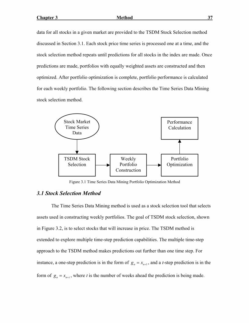
Chapter 3 Method 37
data for all stocks in a given market are provided to the TSDM Stock Selection method
discussed in Section 3.1. Each stock price time series is processed one at a time, and the
stock selection method repeats until predictions for all stocks in the index are made. Once
predictions are made, portfolios with equally weighted assets are constructed and then
optimized. After portfolio optimization is complete, portfolio performance is calculated
for each weekly portfolio. The following section describes the Time Series Data Mining
stock selection method.
Stock MarketTime Series
Data
Performance Calculation
Portfolio Optimization
Weekly Portfolio
Construction
TSDM Stock Selection
Figure 3.1 Time Series Data Mining Portfolio Optimization Method
3.1 Stock Selection Method
The Time Series Data Mining method is used as a stock selection tool that selects
assets used in constructing weekly portfolios. The goal of TSDM stock selection, shown
in Figure 3.2, is to select stocks that will increase in price. The TSDM method is
extended to explore multiple time-step prediction capabilities. The multiple time-step
approach to the TSDM method makes predictions out further than one time step. For
instance, a one-step prediction is in the form of 1n ng x += , and a t-step prediction is in the
form of , where t is the number of weeks ahead the prediction is being made. n ng x += t

Chapter 3 Method 38
TSDM Method
Stock MarketPrice Time
SeriesRepeat for all stocks in an Index
Stock Market Index Data
Predictions on each stock in
the index
Figure 3.2 Time Series Data Min
Following the steps listed in Section 2.4
with different prediction-step lengths. Each sign
patterns are defined using the previous three po
embedding dimension of 3. Events are triggered
temporal pattern in the predictive testing stage i
temporal structure found in the training stage. T
shown,
n tn
xgx
+ +=
allows for a value to be given to a multi-step pr
the Time Series Data Mining Method. This func
the training stage, with event that occur in the f
price.
Once stock selections are made, predicti
A dynamic portfolio matrix, p stocks by N week
TSDM Stock Selection
ing Stock Selection Method
.2, weekly stock predictions are made
al is embedded into a RPS. Temporal
ints of stock closing price data, with an
and opportunities are created if a
s within a region defined by the optimal
he associated percent change function
1 n t
n t
x
+
+− , (3.1)
ediction made during the testing stage of
tion links temporal structures, found in
uture, such as the desired increase in stock
ons are combined into weekly portfolios.
ly time periods, is constructed. Portfolio

Chapter 3 Method 39
assets and performance will be different for each weekly portfolio due to the active
portfolio management approach in which each portfolio is bought at the beginning of the
week and sold at the end of the week. Weekly stock predictions are made with associated
goal function values (weekly stock price percent change) that are either positive,
negative, or zero. A positive prediction value means that the stock price increased. A
negative prediction value means the stock price decreased for that week. A prediction
value of zero means no prediction was made in that week for that stock. The next section
describes the modified portfolio optimization process.
3.2 Modified Portfolio Optimization Method
Once the equal weighted portfolios are created, portfolio optimization techniques
are used to optimize the weekly portfolios. The goal of the portfolio optimization is to
maximize portfolio return for a given level of portfolio risk. As stated earlier, the risk of a
portfolio is defined as the standard deviation of expected returns of the assets in the
portfolio. Modern Portfolio Theory (MPT) provides techniques to adjust the portfolio
weights, to maximize portfolio return for each level of risk.
The efficient frontier of portfolios represents the set of optimal portfolios from
which to choose. To construct an efficient frontier from a given equally weighted
portfolio, a weight adjustment process must be conducted. The weight adjustment process
is a constrained optimization problem formulated by maximizing portfolio return for
given portfolio risk values. The predictive process uses expected returns generated from
the training period signal to create the covariance matrix of expected returns used in
calculating portfolio risk. The covariance matrix represents the variance between

Chapter 3 Method 40
expected returns for each asset in the portfolio. The method iteratively adjusts weight
values using the process listed below:
1. Calculate portfolio return ( ), 1portfolior t t = and portfolio risk ( ), 1portfolio t tσ =
with equally weighted assets.
2. Hold portfolio risk, ( )portfolio tσ , constant and adjust weights ( , to
achieve a higher portfolio return .
1,..., )nw w
( )portfolior t
3. If ∑ and 1( ,..., ) 1, 0, n nw w w= ≠ ∀ n n
t
( ) ( 1), (2,..., )portfolio portfolior t r t t> − =
Continue to adjust portfolio weights to achieve a higher return value.
4. If then ( ) ( 1)portfolio portfolior t r t≤ − max( ( ), ( 1))portfolio portfolio portfolior r t r= − .
Using the Capital Asset Pricing Model (CAPM), portfolio returns and risk can be
separated using the Capital Market Line (CML) equation. Making assumptions about the
risk-free rate of return, a line can be extended from the risk-free rate of return, tangent to
the efficient frontier, constructing the CML. Incorporating previously stated assumptions
of the CAPM, and the derived market portfolio M from the CML, a new portfolio 'M is
now introduced. The new portfolio 'M is the tangent point located on the constructed
CML extended from the risk-free rate of return. The portfolio 'M , shown in Figure 3.3,
is the equivalent, in terms of location on the CML, to the original optimal market
portfolio M, but using only the stocks selected during the Time Series Data Mining stock
selection process. This concept is essential, because it provides the criterion for selecting
an optimal portfolio from the new efficient frontier created by the CML. An optimal
portfolio, for performance calculation purposes, is defined as the optimal market portfolio
'M or the portfolio with the lowest risk if the optimal market portfolio 'M return is less

Chapter 3 Method 41
than the risk-free rate of return fr . The next section presents and explains the complete
Time Series Data Mining Portfolio Optimization Method.
Risk (Stan
Expe
cted
Ret
urn
M
w
Low
High
fr
'M
Lo
Figure 3.3 Model
3.3 Time Series Data Mining Portfol
The combined trading strategy invol
discussed in Section 3.1 to make weekly bu
given stock market index. These predictions
ahead. This prediction process takes the we
prediction using repeated experiment runs w
After the initial stock selection process, the
dard Deviation)High
Market Portfolio 'M
io Optimization Trading Strategy
ves using the TSDM Stock Selection method,
y or do nothing signals for each stock in the
are made for multiple weekly time steps
ekly stock time series data and makes a t-step
ith different prediction time-step parameters.
weekly portfolios are constructed and

Chapter 3 Method 42
optimized using the adapted portfolio optimization techniques discussed in Sections 2.6
and 3.2.
The steps to formulate a trading strategy using the Time Series Data Mining
Portfolio Optimization approach are listed below:
1. Determine entire time range for stock predictions including training period
signal length.
a. Determine portfolio strategy time period (daily, weekly, monthly,
etc.).
2. Determine desired prediction step size . 1t ≥
3. Make stock selections using TSDM stock selection method.
a. Choose stock market index for stock price data set.
b. Define goal function and ranking function.
c. Determine time series embedding and temporal pattern length.
d. Define genetic algorithms parameters (Section 2.4.2).
4. Construct portfolio matrix.
a. p stocks by N time periods.
5. Perform Mean Variance Portfolio Optimization (Sections 2.6 and 3.2).
a. Create efficient frontier.
b. Select an approximate risk-free rate of return.
c. Create Capital Market Line.
d. Select optimal portfolio.
e. Repeat for a. through d. for all weekly portfolios
6. Calculate portfolio and model performance.

Chapter 3 Method 43
Portfolio performance analysis is performed on all generated portfolios for that
time range. Weekly portfolio return performance and total performance are measured and
compared against the overall market performance as a baseline. The TSDM Stock
Selection method prediction accuracy results are compared against the market baseline
prediction accuracy measure. Portfolio performance analysis and results, including return,
risk, transaction cost, prediction accuracy, and Sharpe’s ratio are presented in Chapter 4.

Chapter 4 Evaluation 44
Chapter 4 Evaluation
This chapter presents an evaluation of the combined method discussed in Chapter
3. Historical stock market data is used to evaluate the Time Series Data Mining Portfolio
Optimization (TSDMPO) trading strategy. The data is comprised of stock price time
series of stocks in a particular market index. The chapter contains an explanation of the
TSDMPO trading method stock market application, experimental set-up, and
experimental results including a transaction cost model.
4.1 Stock Market Application
The combined Time Series Data Mining Portfolio Optimization method is used to
identify profitable trading opportunities and create wealth in an active trading
environment. The evaluation of this trading strategy is performed in a simulated market
where stocks are bought on the first trading day of the week and sold on the last trading
day of the week. In applying any trading strategy in an actual market setting, investors
must pay transaction costs in order to trade securities. The weekly trading strategy makes
weekly predictions over specific time ranges and combines the predictions into weekly
portfolios used to increase profit, outperform market return benchmarks, and overcome
transaction costs.
To simulate an active trading environment, investors are able to implement this
trading strategy using large online trading sites such as TDWaterhouse.com, Etrade.com,
and Ameritrade.com, which have allowed various types of investors to set up and easily
manage their own investments. Combining the availability of current financial data
access and the ability to independently manage investments the Time Series Data Mining
Portfolio Optimization method trading strategy is explored in a simulated market

Chapter 4 Evaluation 45
environment where transaction cost are taken into consideration. The investment strategy
takes advantage of predictive stock selection and optimal asset allocation to trade
portfolios weekly. The next section describes the transaction cost model used to
determine simulated model portfolio returns.
4.2 Transaction Cost Model
A transaction is the buying or selling of a security, and transaction costs are those
associated with trading securities [27,36]. When making trades in the stock market,
investors incur transaction costs that are paid for each transaction made. Transaction cost
can erode the total returns gained from investments. These adverse effects must be
considered to determine whether the trading strategy is able not only to increase wealth
but also overcome the associated cost with making those trades. Transaction costs have
two components. One cost is broker commissions or fees that are charges assessed by an
agent in return for arranging the purchase or sale of a security [33-35]. Another cost is the
spread, commonly referred to as bid-ask spread, which is the difference between the ask
price (the price at which an investor is willing to sell a particular security in the
secondary market) and the bid price (the price at which an investor is willing to buy a
particular security in the secondary market) [33-35].
The commission value is determined by the typical price paid to buy or sell shares
of stock at an online trading site such as TDWaterhouse.com or Etrade.com. The
commission per transaction is $10 per stock or $20 for a round trip (buy and sell). A
model for the approximate bid-ask spread was developed by Roll [36]. Assuming that the
markets are efficient and that the probability distribution of observed price changes is
stationary in short intervals, the spread is modeled by the first order covariance of

Chapter 4 Evaluation 46
successive price changes [36]. A modified version the equation is used to model bid-ask
spread and neglects the downward bias in the original equation, which makes spread
values negative [36]. The bid ask spread is modeled as:
2 cov( ( )),nBAS S x= n (4.1)
where nBAS is the bid-ask spread at time index n, and is the stock closing price
training period signal. The total transaction cost for a security at time index t is the
commissions plus the bid-ask spread shown,
( )nS x
,n nTC BAS Cn= + (4.2)
where TC is the transaction cost at time index n, n nBAS is the bid-ask spread at time
index n, and is the commission at time index n. The following section explains the
experiment set-up used in evaluating the TSDMPO trading strategy.
nC
4.3 Experiments
The experiments are divided into groups based on the prediction time-step for
each experiment. Prediction time steps 1, 2, 3, and 4 are used in exploring the multi-step
capabilities of the Time Series Data Mining Stock Selection method. Experiments are
also grouped based on the chosen model testing time range of the chosen data set.
The data set used in the experiments is obtained from http://finance.yahoo.com
and is comprised of weekly stock market data from the Dow Jones Industrial Average.
The Dow Jones Industrial Average (DJIA) is a price-weighted average of thirty large
capital stocks traded on the New York Stock Exchange. The stock listing for the Dow
Jones Industrial Average is shown in Appendix A.1. The stock market data is in the form
of weekly open price, close price, high price, low price, and trading volume. The data set

Chapter 4 Evaluation 47
spans from January 1, 2002 to January 1, 2003 and January 1, 2003 to January 1, 2004.
Theses time ranges were selected to test the method in both bull (generally rising stock
prices) and bear (generally declining stock prices) market conditions.
Time Series Data Mining Stock Selection parameters involving the training period
and genetic algorithm based optimization are held constant through each experiment. The
time series is embedded with a dimension of 3, which creates predictive structures using
the three weeks of closing price data including the current time point and the two
previous points. The initial genetic algorithm population is set to 30 to create a
population large enough for the genetic algorithm to make subsequent solution
generations. The algorithm has halting criterion set to stop the genetic algorithm search
when fitness values converge to a value set at 0.9 multiplied by the maximum fitness
value. The training period is 26 weeks and was chosen by empirically comparing results
of each market index experiment using training ranges varying form 5 weeks to 52
weeks.
Portfolio optimization parameters include the initial portfolio value and the risk-
free rate of return used in calculating model returns and determining optimal portfolio
selection. The initial portfolio value is reset to $100,000 dollars at the beginning of every
trading week to provide a basis on calculating weekly returns and adjustments for
transaction cost. The risk-free rate of return is the 90-day Treasury bill rate of return at
the beginning of the time range. The 90-day Treasury bill rate of return was 1.68 % at
January 1, 2002 and 1.19 % at Jan 1, 2003.

Chapter 4 Evaluation 48
4.4 Results
This section presents results for weekly-optimized portfolios from the Dow Jones
Industrial Average data used in experiments. Optimized portfolios or mean variance
efficient portfolios are defined Chapter 2 and further discussed Chapter 3. These
portfolios are described by the market portfolio 'M defined by the Capital Market Line
defined in Chapter 3. Results from the prediction-step experiments conducted in a stock
market index will be compared to the same complete market index as a benchmark. The
model return results from optimized portfolios generated from stock selection using the
Dow Jones Industrial Average index will be compared against the DJIA index market
rate of return and buy and hold returns. The model risk will be compared using portfolio
beta values, which measure risk relative to the overall market. The index benchmarks are
performance for the entire index, while the model portfolios are specific segments of the
market.
4.4.1 Portfolio Return
Portfolio returns are presented in this section and are defined in Chapters 2 and 3.
Portfolio returns are calculated by using the associated weight values determined from
the portfolio optimization process and described in Sections 3.2 and 3.3. A vector of
optimal portfolio returns,
[ ( ) , 1,..., ]optimal portfolior r n n N= = , (4.3)
contains the optimal portfolio returns for each week over the entire time range T.
The combined model rate of return is the geometric average of weekly portfolio returns
over the entire time range T shown as

Chapter 4 Evaluation 49
1/
1
( ) ( ) 1NN
Modeln
rr n r n=
= − ∏ . (4.4)
The adjusted model rate of return is the combined model rate of return with the average
weekly transaction cost, shown in Section 4.2, subtracted from it denoted by
* 1( ( )
( ) ( )
N
nModel Model
TC nrr n rr n
N=
) = −
∑. (4.5)
The total model return is the product of the adjusted model rate of return for the time
range,
1
( ) 1.N
Model Modeln
R rr n=
= − ∏ (4.6)
Weekly portfolio return values are calculated and then averaged to obtain an overall
performance value for the time range. The average model risk is the mean of all weekly
portfolio risk values over the time range. Tables 4.1 and 4.2 provide numerical results for
the Time Series Data Mining Portfolio Optimization model, using Dow Jones Industrial
Average stock data, with prediction steps 1, 2, 3, and 4.
Dow Jones Industrial Average
Prediction Time-Step
1/01/2002 – 1/01/2003 1 2 3 4 Model Rate of Return 1.898 % 2.112 % 1.105 % 0.894 % Adjusted Model Rate of Return 1.897% 2.111 % 1.104 % 0.893 %
Average Weekly Transaction Cost ($) 97.00 103.00 107.00 97.00
Total Model Return 151.240 % 172.757 % 67.638 % 50.588 %
Table 4.1 Dow Jones Industrial Average Return Performance 1/01/2002 –1/01/2003

Chapter 4 Evaluation 50
The model rate of return was greater than the average market rate of return in the
January 1, 2002 through January 1, 2003 time period. The average weekly market rate of
return was -0.315 % for the time period. This also led to the total model return also being
greater than the market total buy and hold return in the time period. The total market buy
and hold return was –18.070 % for this time period. Average weekly transaction cost had
little effect on overall return performance due to the small number of stocks selected on a
weekly basis and low estimated bid ask spread values.
Dow Jones Industrial Average
Prediction Time-Step
1/01/2003 – 1/01/2004 1 2 3 4 Model Rate of Return 2.249 % 1.876 % 1.704 % 2.302 % Adjusted Model Rate of Return 2.248 % 1.875 % 1.703 % 2.301 %
Average Weekly Transaction Cost($) 104.00 104.00 112.00 106.00
Total Model Return 197.324 % 144.056 % 121.256 % 178.456 %
Table 4.2 Dow Jones Industrial Average Return Performance 1/01/2003 –1/01/2004
The model rate of return was greater than the average market rate of return in the
January 1, 2003 through January 1, 2004 time period. The average weekly market rate of
return was 0.351 % for the time period. This also led to the total model return also being
greater than the market total buy and hold return in the time period. The total market buy
and hold return was 24.333 % for this time period. Average weekly transaction cost were
higher than the previous year due to the model making more selections in better bull
market conditions. However, the transaction cost still had little effect on overall return
performance.
The poor market conditions that existed from January 1, 2002 through January 1,
2003 led to an overall lower performance compared to the results for the time period

Chapter 4 Evaluation 51
spanning from January 1, 2003 through January 1, 2004. In both experiments, the
multiple step predictions were able to provide positive results by outperforming the
overall market and overcoming associated transaction costs. The overall portfolio
performance results were consistent between both experiment time ranges, by showing a
slight decrease in the rate of return as the prediction step increased, except for the
increase in rate of return for prediction step size 2 in year 2002 experiments and the
increase for rate of return in prediction step size of 4 in year 2003 experiments.
Figures 4.1 through 4.4 show the 1, 2, 3, and 4 step cumulative weekly returns for
the TSDMPO model vs. the benchmark for the year 2002. Figures 4.5 through 4.8 show
the 1, 2, 3, and 4 step cumulative weekly returns for the model vs. the benchmark for the
year 2003. The graphical representation of these results shows how the model compares
to the entire market, as a benchmark, over the given time ranges.

Chapter 4 Evaluation 52
5 10 15 20 25 30 35 40 45-50
0
50
100
150
200
Week Number
Wee
kly
Rat
e of
Ret
urn(
%)
Cumulative Weekly Return vs Benchmark
TSDMPO ModelBenchmark Index
Figure 4.1 Dow Jones Industrial Average Portfolio Rate of Return 1/01/2002 – 1/01/2003 One-step prediction
Figure 4.1 represents the one-step TSDMPO model cumulative weekly rate of
return compared with the DJIA index cumulative weekly rate of return. This plot shows
that the TSDMPO model outperforms the benchmark index over the time period. The
model rate of return is lower than the benchmark for a very brief period of weeks early in
the time period and performs very strongly later in the time period. The one-step
prediction model shows greater rate of return volatility than the market as show by Figure
4.1 with larger moves in cumulative weekly return. The model’s largest one week loss
was 18.08% during week 26, and the model’s largest one week gain was 26.63% during
week 40, for this time period.

Chapter 4 Evaluation 53
5 10 15 20 25 30 35 40 45-50
0
50
100
150
200
Week Number
Wee
kly
Rat
e of
Ret
urn(
%)
Cumulative Weekly Return vs Benchmark
TSDMPO ModelBenchmark Index
Figure 4.2 Dow Jones Industrial Average Portfolio Rate of Return
1/01/2002 – 1/01/2003 Two-step prediction
Figure 4.2 represents the two-step TSDMPO model cumulative weekly rate of
return compared with the DJIA index weekly rate of return. This plot shows that the
TSDMPO model outperforms the benchmark index over the time period. The total model
rate of return never goes lower than the rate of return benchmark index and has strong
performance in the second half of the year. The two-step prediction model shows greater
rate of return volatility than the market as show by Figure 4.2, but does not show as much
volatility as the one-step prediction model. The model’s largest one week loss was
13.56% during week 46, and the model’s largest one week gain was 26.07% during week
39, for this time period.

Chapter 4 Evaluation 54
5 10 15 20 25 30 35 40 45-50
0
50
100
150
200
Week Number
Wee
kly
Rat
e of
Ret
urn(
%)
Cumulative Weekly Return vs Benchmark
TSDMPO ModelBenchmark Index
Figure 4.3 Dow Jones Industrial Average Portfolio Rate of Return
1/01/2002 – 1/01/2003 Three-step prediction
Figure 4.3 represents the three-step TSDMPO model cumulative weekly rate of
return compared with the DJIA index weekly rate of return. This plot shows that the
TSDMPO model outperforms the benchmark index over the time period. The total model
rate of return has periods of under performance in the first half of the time period, but
performs stronger later in the time period by outperforming the market rate of return
benchmark. The three-step prediction model shows greater rate of return volatility than
the market as show by Figure 4.3, but shows less volatility than the one-step and two-step
prediction models. The model’s largest one week loss was 16.92% during week 31, and
the model’s largest one week gain was 12.80% during week 26, for this time period.
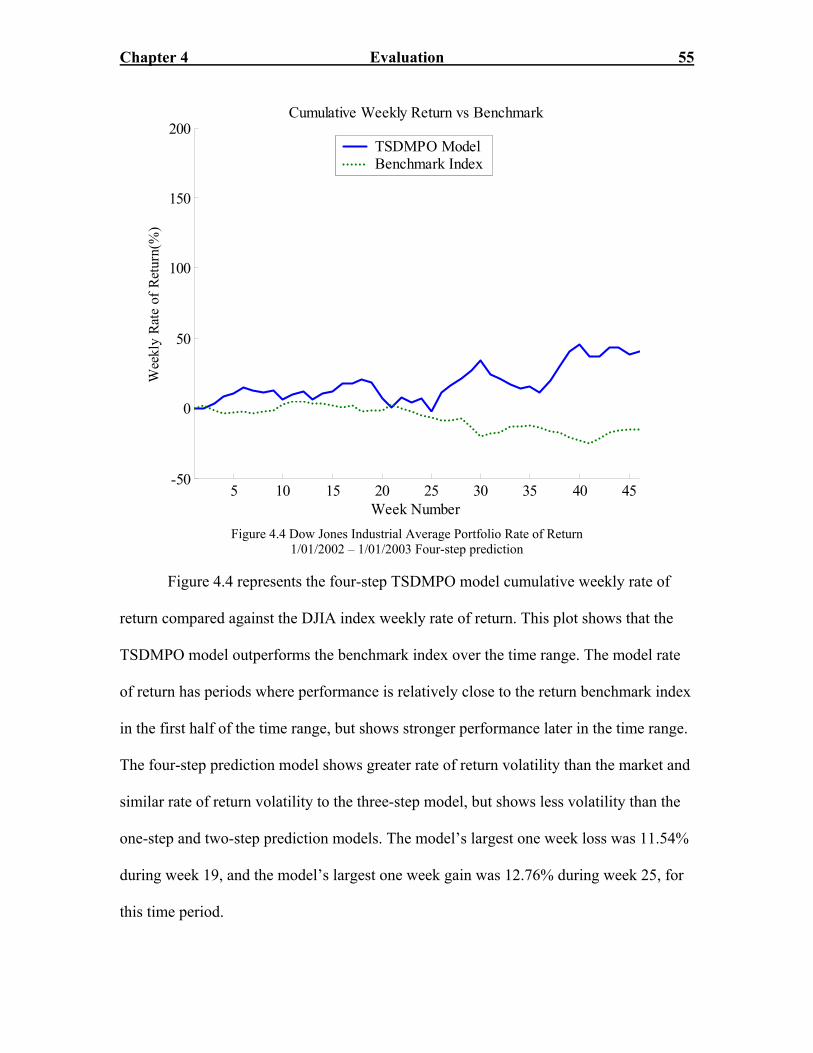
Chapter 4 Evaluation 55
5 10 15 20 25 30 35 40 45-50
0
50
100
150
200
Week Number
Wee
kly
Rate
of R
etur
n(%
)
Cumulative Weekly Return vs Benchmark
TSDMPO ModelBenchmark Index
Figure 4.4 Dow Jones Industrial Average Portfolio Rate of Return
1/01/2002 – 1/01/2003 Four-step prediction
Figure 4.4 represents the four-step TSDMPO model cumulative weekly rate of
return compared against the DJIA index weekly rate of return. This plot shows that the
TSDMPO model outperforms the benchmark index over the time range. The model rate
of return has periods where performance is relatively close to the return benchmark index
in the first half of the time range, but shows stronger performance later in the time range.
The four-step prediction model shows greater rate of return volatility than the market and
similar rate of return volatility to the three-step model, but shows less volatility than the
one-step and two-step prediction models. The model’s largest one week loss was 11.54%
during week 19, and the model’s largest one week gain was 12.76% during week 25, for
this time period.

Chapter 4 Evaluation 56
5 10 15 20 25 30 35 40 45-50
0
50
100
150
200
Week Number
Wee
kly
Rat
e of
Ret
urn(
%)
Cumulative Weekly Return vs Benchmark
TSDMPO ModelBenchmark Index
Figure 4.5 Dow Jones Industrial Average Portfolio Rate of Return
1/01/2003 – 1/01/2004 One-step prediction
Figure 4.5 represents the one-step TSDMPO model cumulative weekly rate of
return compared against the DJIA index weekly rate of return. This plot shows that the
TSDMPO model outperforms the benchmark index over the time range. The model rate
of return has periods where performance is lower that the rate of return benchmark index
early in the time range, but outperforms the benchmark significantly later in the time
range. The one-step prediction model shows greater rate of return volatility than the
market, but the majority of the volatility is in the positive direction. The model’s largest
one week loss was 6.35% during week 1, and the model’s largest one week gain was
14.90% during week 38, for this time period.

Chapter 4 Evaluation 57
5 10 15 20 25 30 35 40 45-50
0
50
100
150
200
Week Number
Wee
kly
Rate
of R
etur
n(%
)
Cumulative Weekly Return vs Benchmark
TSDMPO ModelBenchmark Index
Figure 4.6 Dow Jones Industrial Average Portfolio Rate of Return
1/01/2003 – 1/01/2004 Two-step prediction
Figure 4.6 represents the one-step TSDMPO model cumulative weekly rate of
return compared against the DJIA index weekly rate of return. This plot shows that the
TSDMPO model outperforms the benchmark index over the time range. The model rate
of return has periods where performance is slightly lower that the rate of return
benchmark index early in the time range, but then quickly outperforms the benchmark
throughout the time range. The two-step prediction model shows greater rate of return
volatility than the market and has similar volatility to the one-step prediction model. The
model’s largest one week loss was 8.30% during week 10, and the model’s largest one
week gain was 12.67% during week 47, for this time period.
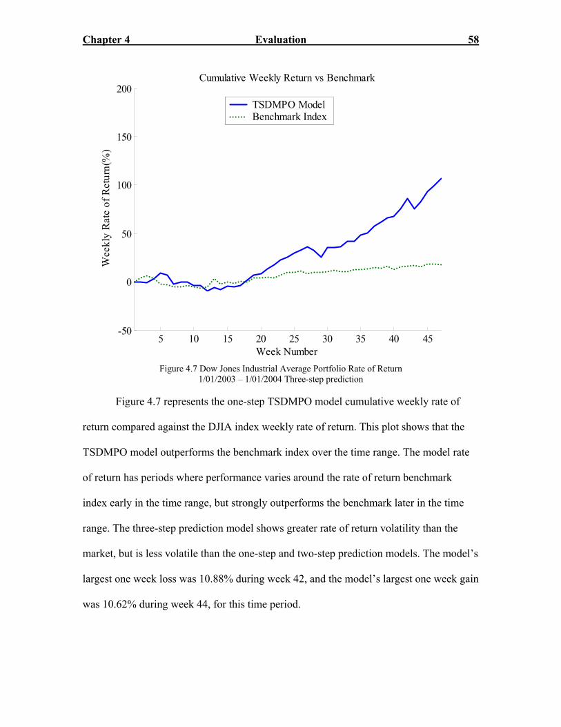
Chapter 4 Evaluation 58
5 10 15 20 25 30 35 40 45-50
0
50
100
150
200
Week Number
Wee
kly
Rat
e of
Ret
urn(
%)
Cumulative Weekly Return vs Benchmark
TSDMPO ModelBenchmark Index
Figure 4.7 Dow Jones Industrial Average Portfolio Rate of Return
1/01/2003 – 1/01/2004 Three-step prediction
Figure 4.7 represents the one-step TSDMPO model cumulative weekly rate of
return compared against the DJIA index weekly rate of return. This plot shows that the
TSDMPO model outperforms the benchmark index over the time range. The model rate
of return has periods where performance varies around the rate of return benchmark
index early in the time range, but strongly outperforms the benchmark later in the time
range. The three-step prediction model shows greater rate of return volatility than the
market, but is less volatile than the one-step and two-step prediction models. The model’s
largest one week loss was 10.88% during week 42, and the model’s largest one week gain
was 10.62% during week 44, for this time period.
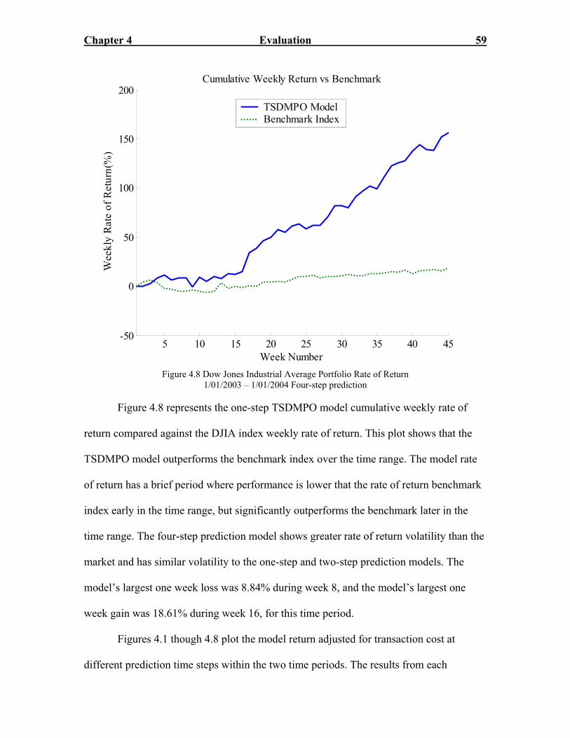
Chapter 4 Evaluation 59
5 10 15 20 25 30 35 40 45-50
0
50
100
150
200
Week Number
Wee
kly
Rat
e of
Ret
urn(
%)
Cumulative Weekly Return vs Benchmark
TSDMPO ModelBenchmark Index
Figure 4.8 Dow Jones Industrial Average Portfolio Rate of Return
1/01/2003 – 1/01/2004 Four-step prediction
Figure 4.8 represents the one-step TSDMPO model cumulative weekly rate of
return compared against the DJIA index weekly rate of return. This plot shows that the
TSDMPO model outperforms the benchmark index over the time range. The model rate
of return has a brief period where performance is lower that the rate of return benchmark
index early in the time range, but significantly outperforms the benchmark later in the
time range. The four-step prediction model shows greater rate of return volatility than the
market and has similar volatility to the one-step and two-step prediction models. The
model’s largest one week loss was 8.84% during week 8, and the model’s largest one
week gain was 18.61% during week 16, for this time period.
Figures 4.1 though 4.8 plot the model return adjusted for transaction cost at
different prediction time steps within the two time periods. The results from each

Chapter 4 Evaluation 60
experiment are consistent with numerical results and show the model outperforming the
market benchmark as time continues. From January 1, 2002 through January 1, 2003, the
return performance was positive despite negative market conditions. From January 1,
2003 through January 1, 2004, the return performance improved over the previous year’s
performance in three out of four prediction time steps.
Figure 4.9 shows an example of an observed optimal portfolio that occurred in
2003 using the TSDMPO trading strategy with a one-step prediction. This visual
representation shows the selection of an optimal portfolio, which is theoretically
explained in Section 2.6. The Optimal Risk Portfolio 'M represents the optimal portfolio
selected during experimentation. The graph also shows the Capital Market Line
extending from the risk-free rate of return, fr at 1.19 %. The next section evaluates
portfolio risk and overall model risk performance. The next section presents model
portfolio risk results.

Chapter 4 Evaluation 61
0 1 2 3 4 5 60.0115
0.012
0.0125
0.013
0.0135
0.014
0.0145Optimal Capital Allocation
Risk (Standard Deviation)
Expe
cted
Ret
urn
M'
fr
Figure 4.9 Observed Optimal Portfolio w/Efficient Frontier
4.4.2 Portfolio Risk
An evaluation of model portfolio risk is presented in this section. The risk of a
portfolio can be determined in various ways. Traditional modern portfolio theory
determines risk, a posteriori, as the variance and standard deviation of expected returns.
The Capital Asset Pricing Model determines risk in terms of beta, β. Portfolio risk,
portfolioσ , and portfolio beta, portfolioβ , are defined in Chapters 2 and 3. Other popular
measures of risk have emerged and will allow for further risk analysis of the weekly
portfolios created during the Time Series Data Mining Portfolio Optimization method.
The Sharpe’s Ratio is calculated to further analyze the risk vs. return of generated weekly
portfolios.

Chapter 4 Evaluation 62
The Sharpe’s ratio is a ratio developed by William Sharpe in 1966 to measure
risk-adjusted performance [37]. The risk adjusted return measures how much risk a
portfolio assumes to earn its returns. This is usually expressed as a number or a rating.
The Sharpe’s ratio sr is defined as,
,portfolio f
portfolio
r rsr
σ−
= (4.7)
where is the model average portfolio return, portfolior fr is the market rate of return,
and portfolioσ is the average portfolio standard deviation for the time range. The Sharpe
ratio determines whether the returns of a portfolio are because of wise investment
decisions or a result of taking excess risk. This ratio is useful in comparing portfolios and
assets in terms of volatility to return. A high Sharpe’s Ratio implies the portfolio or stock
is realizing sufficient or good returns for each unit of risk. The measure is used here to
evaluate the model average portfolio return and risk results.
Tables 4.3 and 4.4 contain model portfolio risk results. Weekly portfolio risk
values are calculated for each risk measure. These weekly values are averaged to obtain
an overall performance value for the time range. The average portfolio risk is the mean of
all weekly portfolio risk values portfolioσ over the time range. The average portfolio beta is
the mean of all beta values portfolioβ over the time range. The Shape’s Ratio is calculated
using adjusted model rate of return, risk-free rate of return and, average model risk.

Chapter 4 Evaluation 63
DJIA Prediction Time-Step 1/01/2002 – 1/01/2003
1 2 3 4
Average Portfolio Risk 3.526 3.299 2.956 3.106
Average Portfolio Beta 2.534 2.692 2.471 2.620
Model Sharpe’s Ratio
3.973 4.544 2.615 1.999
Table 4.3 Dow Jones Industrial Average Risk Analysis 1/01/2002 – 1/01/2003
DJIA Prediction Time-Step 1/01/2003 – 1/01/2004
1 2 3 4
Average Portfolio Risk 2.608 3.006 2.683 2.656
Average Portfolio Beta 2.051 2.113 1.626 2.610
Model Sharpe’s Ratio
6.152 4.443 4.515 6.18
Table 4.4 Dow Jones Industrial Average Risk Analysis 1/01/2003 – 1/01/2004
The average portfolio risk values for each prediction step are similar to each
other, with an overall model average of 3.22 in 2002 experiments and 2.74 in 2003
experiments. The average portfolio betas for each prediction step are also similar to each
other, with an overall model average of 2.58 in the 2002 experiments and 2.10 in 2003
experiments. The Sharpe’s ratio value reported is the average value over the time range,
and results do not assume that model portfolio returns must exceed the risk-free rate of
return given by the 90-day Treasury bill at the start of each period, with 1.68 % on
January 1, 2002 and 1.19 % on January 1, 2003. The average Sharpe’ ratio was 3.28 for
year 2002 experiments and 5.32 for year 2003 experiments. Sharpe’s ratio values greater
than one are good, and values greater than two are outstanding. This implies that

Chapter 4 Evaluation 64
experimental results were better than outstanding [43]. The next section shows portfolio
prediction accuracy results.
4.4.3 Prediction Accuracy
During the testing stage of the Time Series Data Mining (TSDM) method,
predictions are evaluated. Stock predictions are made and then given values that are
either positive, negative, or zero. A positive prediction value means that stock price went
up, and a negative prediction value means the stock price went down for the week. The
underlying TSDM trading objective is to find patterns that are predictive of increases in a
stock price. Determining prediction accuracy of the stock selection process is another
indicator of how much risk is taken in investing in these portfolios. If the stock selection
tool is making accurate predictions for positive trading opportunities, then there is less
inherent risk in making trades based on the model. The ratio between the number positive
trades and the number of negative trades is an important measure to determine whether
the stock selection process is accurate given any market conditions. If market conditions
are good, the stock selection should be able to select more stocks with positive gains to
add to a weekly portfolio. In contrast, if market conditions are poor, the model may select
fewer if any stocks to add to the weekly portfolios.
The prediction accuracy also plays a role in the risk of each portfolio. If the
predictions are more accurate, there is less unsystematic risk present in each weekly
portfolio. In comparison to the market baseline positive prediction accuracy, if the model
prediction accuracy is higher, there is less risk than the market in our portfolios.

Chapter 4 Evaluation 65
The prediction accuracy determines the total number of trades in a given time
index n and gives a percent value equal to the ratio between the number of positive trades
and the total number of trades made for that week. The prediction accuracy is defined as
,nn
n
PTPTN
= (4.8)
where is the number of positive trades, and TN is the total number of trades in the
current week n. The total prediction accuracy is an average of the weekly prediction
accuracies over the entire time range T denoted by
nPT n
1 .
N
nn
avg
PP
N==∑
(4.9)
The model percent accuracy is measured against a complete market baseline percent
accuracy. The market baseline percent accuracy measure incorporates all possible weekly
trades for the time period and determines the number of weekly trades that had positive
percent gains and negative percent gains. This comparison gives a baseline against which
to measure how well our prediction accuracy fares against purchasing all given assets in a
market index. Tables 4.5 and 4.6 include results on the model and market accuracy.
DJIA Prediction Time-Step 1/01/2002 – 1/01/2003
1 2 3 4
Positive Model Accuracy 0.500 % 0.445 % 0.412 % 0.383 %
Positive Market Baseline
0.452 % 0.452 % 0.452 % 0.452 %
Table 4.5 Prediction Accuracy Analysis 1/01/2002 – 1/01/2003

Chapter 4 Evaluation 66
DJIA Prediction Time-Step 1/01/2003 – 1/01/2004
1 2 3 4
Positive Model Accuracy 0.594 % 0.515 % 0.569 % 0.550 %
Positive Market Baseline
0.537 % 0.537 % 0.537 % 0.537 %
Table 4.6 Prediction Accuracy Analysis 1/01/2003 – 1/01/2004
The prediction accuracy for the model was greater than the market baseline
accuracy in the one-step prediction, with date range January 1, 2002 through January 1,
2003, experiment. In addition, this was the only experiment out of the four prediction
model experiments with date range, January 1, 2002 through January 1, 2003, that had
prediction accuracy greater than the market baseline accuracy. In contrast, three out of
the four prediction model experiments with date range, January 1, 2003 through January
1, 2004, had prediction accuracies greater than the market baseline accuracy. The next
chapter concludes the thesis, providing insights into the work and future research
directions.
Chapter 5 Conclusions and Future Work 67
Chapter 5 Conclusions and Future Work
This thesis presents a profitable stock trading strategy by combining a temporal
data mining based stock selection approach with portfolio optimization techniques. The
background information for these techniques are found in Chapter 2. The combined
method and trading strategy details are discussed in Chapter 3. Research conclusions
include comparisons and discussions of results, presented in Chapter 4, to provide an
insight and a summary of the research. Future work recommendations, to continue
progress made by this thesis, are provided at the end of this chapter.
5.1 Research Conclusions
The combined Time Series Data Mining Portfolio Optimization model was able to
overcome transaction cost and outperform the market benchmark returns in all prediction
steps for two time periods spanning from January 1, 2002 to January 1, 2003 and from
January 1, 2003 to January 1, 2004. The prediction model is capable of looking further
ahead and making predictions that are further out than one-step and achieve desired
results. This predictive ability allows investors to make longer-term decisions and
possibly avoid additional transaction cost due to fewer transactions. The success of the
multi-step approach shows the stock selection model’s predictive ability to select stocks
with positive returns over various prediction horizons.
In further evaluating the TSDM stock selection method, model prediction
accuracies also demonstrated that the stock selection method has predictive ability.
Prediction accuracy results show that the model prediction accuracy was lower in year
2002 experiments than in year 2003 experiments. The model had higher prediction
accuracy than the market baseline in four out of eight total experiments, with three of

Chapter 5 Conclusions and Future Work 68
those accuracy measurements coming in year 2003 experiments, which experienced
favorable market conditions. The stock selection model has the capability to work better
in good market conditions, while still achieving desired return performance in both good
and bad overall market conditions.
When considering prediction accuracy as a part of portfolio risk, due to an
investor’s ability to make positive or negative portfolio stock selections, the model
assumed more risk in the year 2002 experiments than it did in the year 2003 experiments,
due to the lower accuracy levels. Year 2002 experiments averaged 43.5% accuracy and
year 2003 averaged 55.7% accuracy. The year 2002 had overall bad market conditions.
These market conditions forced the combined model to take on more portfolio risk to
achieve positive returns in Chapter 4. The model also took on more risk, in a traditional
sense, shown by the portfolio beta values. The model average beta risk values were at
least two times greater (2.58 and 2.10) than the market beta, which has a beta value of 1.
The model beta values show that generated portfolios on average have a higher risk level
than the overall market. This risk is mainly due to a lack of diversification in weekly
portfolios. The generated model portfolios have fewer stocks in them than the number of
stocks in the overall benchmark index.
The returns of the initial stock portfolios are improved using the portfolio
optimization techniques discussed in Section 3.2. The process of rebalancing the portfolio
weights to achieve better risk vs. return characteristics also contributes to the overall
model return. The optimal portfolios constructed have better risk vs. return characteristics
than portfolios that are not optimized with the same set of assets. This has been
demonstrated both in theory and now in practice using the Time Series Data Mining

Chapter 5 Conclusions and Future Work 69
Portfolio Optimization trading strategy. As stated in Chapter 4, returns are calculated
based on a $100,000 portfolio value with an adjustment for the transaction cost associated
with the weekly trading strategy. Transaction cost will have more of an effect on the
overall portfolio return if the initial weekly portfolio value is lower than $100,000 and
less of an effect if the initial weekly portfolio value is higher than $100,000. Due to
higher portfolio values, more shares of each stock can be purchased and added to a
portfolio producing higher overall returns.
The combined TSDMPO model achieved all previously stated goals including
outperforming the overall market in bull (good) and bear (bad) market conditions. This
trading strategy can now be used to trade in an actual market setting using all widely
available and frequently traded stocks with sufficient data resources. Using the TSDMPO
trading strategy on a weekly basis helps overcome transaction cost associated with
trading and allows an investor to realize profits over a given time range. The results
presented here are for a one-year time period, but could be extended for longer time
periods to obtain similar results due to the adaptive nature of the stock selection method.
The next section discusses future work to continue the research presented in this thesis.
5.2 Future Work
Future work lies in the area of extending the predictive capabilities of the Time
Series Data Mining stock selection method, incorporating short selling strategies, and
investigating options data sets. The TSDM stock selection method could be extended to
use multiple predictive structures with various lengths. These multiple predictive
structures with various lengths will require higher embedding dimensions to capture
temporal patterns in the reconstructed phase space.

Chapter 5 Conclusions and Future Work 70
The use of options data should also be considered in trying to make predictions
and developing trading strategies. Using the actual options price data or the underlying
option strike price data are two possible data sets that could be used to make stock
selections from. Also return performance could be calculated using either the underlying
stock price of the option or the actual option prices.
The current work focuses on a long trading strategy. Trading long is exactly like
the trading performed in this thesis, in which a stock is bought and held to be sold later at
a higher price. Short selling is the selling of a security that an investor does not currently
own, and the transaction is completed by the purchase and delivery of a security
borrowed by the seller [5]. A short selling strategy profits from being able to buy the
stock at a lower price than the price at which they sold short. Incorporating a short selling
strategy should be investigated to see if changing the model objective can achieve results
that are similar those reported in this research.

References 71
[1] R. C. Grinold and R. N. Kahn, Active Portfolio Management, Second ed. New
York: McGraw-Hill 2000.
[2] D. R. Emery, J. D. Finnerty, and J. D. Stowe, Corporate Financial Management,
Second ed. Upper Saddle River: Pearson Education, 2004.
[3] R. J. Povinelli, "Time Series Data Mining: Identifying Temporal Patterns for
Characterization and Prediction of Time Series Events," in Electrical and
Computer Engineering. Milwaukee: Marquette University, 1999.
[4] G. E. P. Box and G. M. Jenkins, Time Series Analysis: Forecasting and Control,
Rev. ed. San Francisco: Holden-Day, 1976.
[5] F. K. Reily and K. C. Brown, Investment Analysis and Portfolio Management, 7th
ed. Mason, OH: Thomson Learning, 2003.
[6] G. Deboeck, Trading on the Edge, Canada: Wiley and Sons, 1994.
[7] F. J. Fabozzi, Handbook of Portfolio Management. New Hope: Frank J. Fabozzi
Associates, 1998.
[8] J. Richard and J. Bauer, Genetic Algorithms and Investment Strategies: Karl
Weber, 1994.
[9] H. Markowitz, "Portfolio Selection," Journal of Finance, vol. 7, pp. 77 -91, 1952.
[10] R. J. Povinelli, "Identifying Temporal Patterns for Characterization and Prediction
of Financial Time Series Events," presented at Temporal, Spatial and Spatio-
Temporal Data Mining: First International Workshop; TSDM2000, Lyon, France,
2000.
[11] F. M. Roberts, R. J. Povinelli, and K. M. Ropella, "Identification of ECG
Arrhythmias using Phase Space Reconstruction," presented at Principles and

References 72
Practice of Knowledge Discovery in Databases (PKDD'01), Freiburg, Germany,
2001.
[12] K. M. Indrebo, R. J. Povinelli, and M. T. Johnson, "A Combined Sub-band and
Reconstructed Phase Space Approach to Phoneme Classification," presented at
ISCA Tutorial and Research Workshop on Non-linear Speech Processing
(NOLISP), Le Croisic, France, 2003.
[13] M. T. Johnson, A. C. Lindgren, R. J. Povinelli, and X. Yuan, "Performance of
Nonlinear Speech Enhancement using Phase Space Reconstruction," presented at
International Conference on Acoustics, Speech and Signal Processing, Hong
Kong, 2003.
[14] M. Duan and R. J. Povinelli, "Estimating Stock Price Predictability Using Genetic
Programming," presented at Genetic and Evolutionary Computation Conference
(GECCO-2001), San Francisco, California, 2001.
[15] I. H. Witten and E. Frank, Data mining: practical machine learning tools and
techniques with Java implementations. San Francisco, California: Morgan
Kaufmann, 2000.
[16] U. Fayyad and R. Uthurusamy, "Data Mining and Knowledge Discovery in
Databases," Communications of the ACM, vol. 39, pp. 24-26, 1996.
[17] T. M. Mitchell, Machine Learning. New York: McGraw-Hill, 1997.
[18] W. Lin, M. A. Orgun, and G. J. Williams, "An Overview of Temporal Data
Mining," presented at Australasian Data Mining Conference, University House,
ANU, Canberra, 2002.
[19] H. D. I. Abarbanel, Analysis of observed chaotic data. New York: Springer, 1996.

References 73
[20] H. Kantz and T. Schreiber, Nonlinear time series analysis. Cambridge:
Cambridge University Press, 1997.
[21] F. Takens, "Detecting strange attractors in turbulence," presented at Dynamical
Systems and Turbulence, Warwick, 1980.
[22] T. Sauer, "Time series prediction using delay coordinate embedding," in Time
Series Prediction: Forecasting the Future and Understanding the Past, A. S.
Weigend and N. A. Gershenfeld, Eds.: Addison-Wesley, 1994, pp. 175-194.
[23] T. Sauer, J. A. Yorke, and M. Casdagli, "Embedology," Journal of Statistical
Physics, vol. 65, pp. 579-616, 1991.
[24] D. E. Goldberg, Genetic algorithms in search, optimization, and machine
learning. Reading, Massachusetts: Addison-Wesley, 1989.
[25] R. J. Povinelli and X. Feng, "Temporal Pattern Identification of Time Series Data
using Pattern Wavelets and Genetic Algorithms," presented at Artificial Neural
Networks in Engineering, St. Louis, Missouri, 1998.
[26] R. J. Povinelli, "Characterization and Prediction of Welding Droplet Release
using Time Series Data Mining," presented at Artificial Neural Networks in
Engineering, St. Louis, Missouri, 2000.
[27] D. Diggs, "A Temporal Pattern Approach for Predicting Weekly Financial Time
Series," presented at Artificial Neural Networks in Engineering, St. Louis,
Missouri, 2003.
[28] R. J. Povinelli and X. Feng, "A New Temporal Pattern Identification Method for
Characterization and Prediction of Complex Time Series Events," IEEE
Transactions on Knowledge & Data Engineering, vol. 15, pp. 339-352, 2003.

References 74
[29] R. J. Povinelli and X. Feng, "Improving Genetic Algorithms Performance By
Hashing Fitness Values," presented at Artificial Neural Networks in Engineering,
St. Louis, Missouri, 1999.
[30] R. J. Povinelli, "Comparing Genetic Algorithms Computational Performance
Improvement Techniques," presented at Artificial Neural Networks in
Engineering, St. Louis, Missouri, 2000.
[31] R. J. Povinelli, "Improving Computational Performance of Genetic Algorithms: A
Comparison of Techniques," presented at Genetic and Evolutionary Computation
Conference (GECCO-2000) Late Breaking Papers, Las Vegas, Nevada, 2000.
[32] H. R. Stoll, "Portfolio Trading," The Journal of Portfolio Management, pp. 20-24,
1998.
[33] H. Markowitz, "Foundations of Portfolio Theory," Journal of Finance, vol. 46,
pp. 469-477, 1991.
[34] H. Markowitz, Portfolio Selection: John Wiley & Sons, Inc., 1959.
[35] M. C. Steinbach, "Markowitz Revisited: Mean-Variance Models in Financial
Portfolio Analysis," Society for Industrial and Applied Mathematics, vol. 43, pp.
31-85, 2001.
[36] R. C. Merton, "An Intertemporal Capital Asset Pricing Model," Economertrica,
vol. 41, pp. 867-887, 1973.
[37] W. F. Sharpe, "Capital Asset Prices with and without Negative Holdings," The
Journal of Finance, vol. 46, pp. 489-509, 1991.
[38] R. Roll, "A simple Implicit Measure of the Effective Bid-Ask Spread in an
Efficient Market," The Journal of Finance, vol. 39, pp. 1127-1139, 1984.

References 75
[39] T. J. George, G. Kaul, and M. Nimalendran, "Estimation of the Bid Ask Spread
and Its Components: A New Approach," The Review of Financial Studies, vol. 4,
pp. 623-656, 1991.
[40] H. R. Stoll, "Inferring the Components of the Bid-Ask Spread: Theory and
Empirical Tests," Journal of Finance, vol. 44, pp. 115 -134, 1989.
[41] C. Klijn, "What determines the bid-ask spread? An introduction in micro structure
economics concerning trading mechanisms," 2001.
[42] W. F. Sharpe, "The Sharpe Ratio," The Journal of Portfolio Management, pp. 49-
58, 1994.
[[43] B. Fulks, "The Sharpe Ratio," investopedia.com, 1998

Appendix 76
Appendix
A.1 Dow Jones 30 Market Index Stock Listings (as of 1/01/2004)
Alcoa - AA
American Express - AXP
AT&T - T
Boeing - BA
Caterpillar - CAT
Coca-Cola - KO
Citigroup - C
Disney - DIS
DuPont - DD
Eastman Kodak - EK
Exxon Mobil - XOM
General Electric - GE
General Motors - GM
Hewlett-Packard - HWP
Home Depot - HD
Honeywell - HON
IBM - IBM
Intel - INTC
International Paper - IP
Johnson & Johnson - JNJ

Appendix 77
McDonald's - MCD
Merck - MRK
Microsoft - MSFT
3M - MMM
JP Morgan - JPM
Philip Morris - MO
Proctor & Gamble - PG
SBC Communications - SBC
United Tech - UTX
Wal-Mart - WMT