Multiple Regression

Farrokh Alemi, Ph.D.

Kashif Haqqi M.D.

Additional Reading

• For additional reading see Chapter 15 and Chapter 14 in Michael R. Middleton’s Data Analysis Using Excel, Duxbury Thompson Publishers, 2000.

• Example described in this lecture is based in part on Chapter 17 and Chapter 18 of Keller and Warrack’s Statistics for Management and Economics. Fifth Edition, Duxbury Thompson Learning Publisher, 2000.

Objectives

• To learn the assumptions behind and the interpretation of multiple variable regression.

• To use Excel to calculate multiple regression.

• To test hypothesis using multiple regression.

Multiple Regression Model

• We assume that k independent variables are potentially related to the dependent variable using the following equation:

• The objective is to find such that the difference between y and is minimized if: = b0 + b1x1 + b2x2 + … + bkxky

y

y = 0 + 1x1 + 2x2 + … + kxk + b0, b1, … bk

Similarity With Single Variable Regression

• Same method of finding best fit with data by minimizing sum of square of residuals

• Same assumptions regarding Normal distribution of residuals and constant standard deviation of residuals

• New issues related to finding optimal combination of variables that can predict response variable

Multiple Regression in Excel

• Arrange y and x variables as columns with each case as a row

• Select tools, data analysis, regression

• Enter the range for Y variable

• Enter the range for all X values

• Select output range and at a minimum select for output normal plot and residual plots

Example• Examine which variable affects the profitability

of health centers. Download data • Regress profit measure (profit divided by

revenue) on:(1) Number of visits

(2) Maximum distance among clinics in the center

(3) Number of employers in the area

(4) Percent of community enrolled in college

(5) Median income of community in thousands

(6) Distance to downtown

Regression Statistics

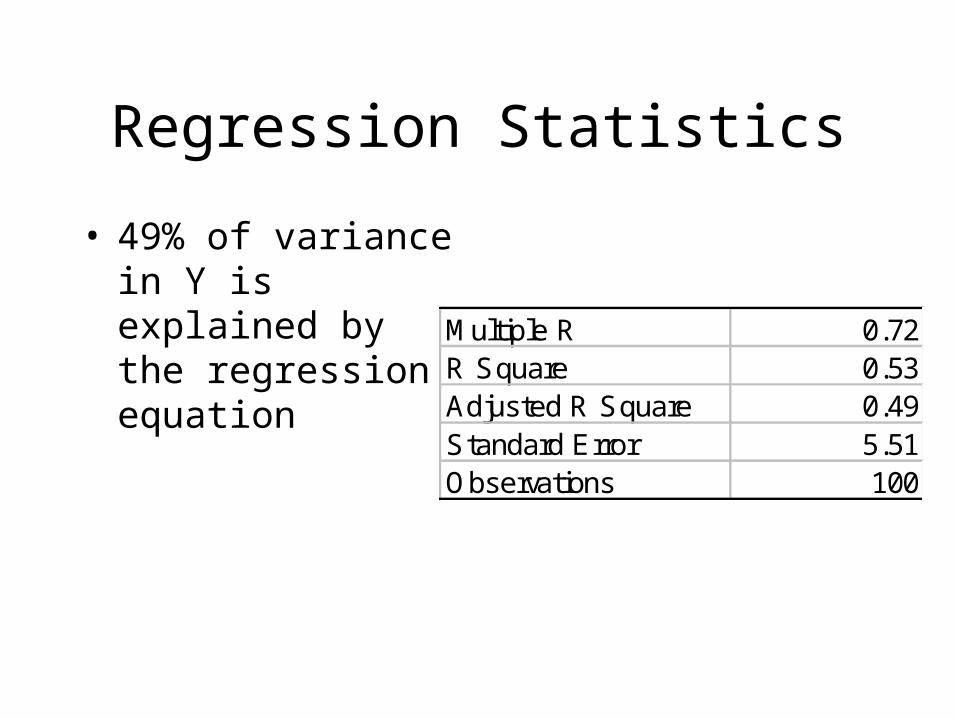
• 49% of variance in Y is explained by the regression equation Multiple R 0.72

R Square 0.53Adjusted R Square 0.49Standard Error 5.51Observations 100

ANOVA for Regression

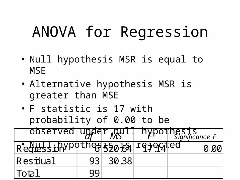
• Null hypothesis MSR is equal to MSE• Alternative hypothesis MSR is greater than

MSE• F statistic is 17 with probability of 0.00 to be

observed under null hypothesis• Null hypothesis is rejected

df MS F Significance F

Regression 6 520.64 17.14 0.00Residual 93 30.38Total 99

Analysis of Coefficients

• Null hypotheses: Coefficients are zero

• Alternative hypothesis: coefficients are different from zero

• Are P values below 0.05?

• All null hypotheses are rejected except college enrollment and distance to downtown

Coefficients t Stat P-valueIntercept 72.45 9.18 0.00Number of visits to competitors -0.01 -6.07 0.00Maximum distance among clinic offices -1.65 -2.60 0.01Number of employers in the area 0.02 5.80 0.00Percent of community enrolled in College 0.21 1.59 0.12Median income in thousands -0.41 -2.96 0.00Distance to downtown 0.23 1.26 0.21

Discussion of Direction of Coefficients

• One visit to the competitor decreases operating margin by 0.01

• One more mile distance among clinics decreases operating margin by 1.65

• One more employer in the community increases operating margin by 0.02

• One thousand dollars more income decreases operating margin by 0.41

Coefficients t Stat P-valueIntercept 72.45 9.18 0.00Number of visits to competitors -0.01 -6.07 0.00Maximum distance among clinic offices -1.65 -2.60 0.01Number of employers in the area 0.02 5.80 0.00Percent of community enrolled in College 0.21 1.59 0.12Median income in thousands -0.41 -2.96 0.00Distance to downtown 0.23 1.26 0.21

Check Assumptions

1. Does the residual have a Normal distribution?

2. Is variance of residuals is constant?

3. Are errors independent?

4. Are there observations that are inaccurate or do not belong to the target population?

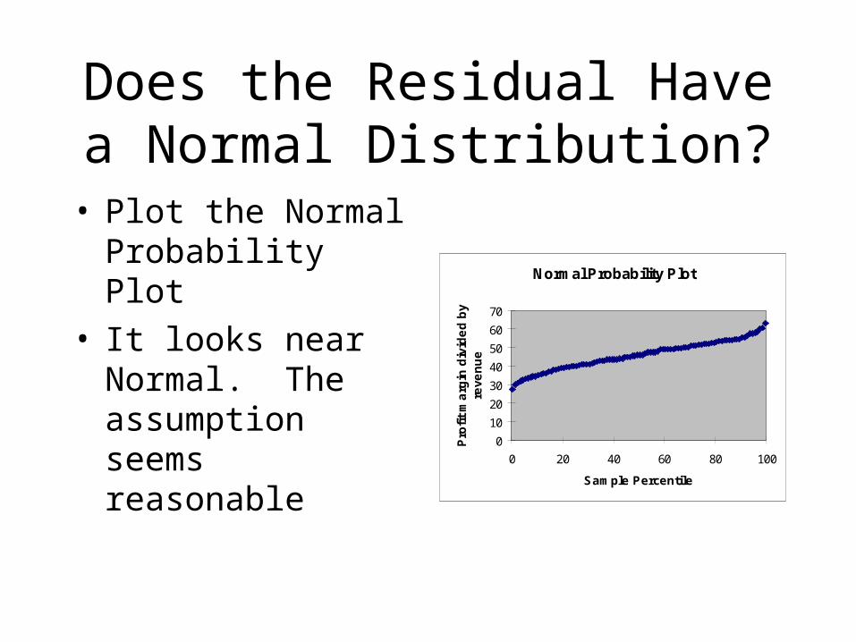
Does the Residual Have a Normal Distribution?

• Plot the Normal Probability Plot

• It looks near Normal. The assumption seems reasonable

Normal Probability Plot

0

10

20

30

40

50

60

70

0 20 40 60 80 100

Sample Percentile

Pro

fit

ma

rgin

div

ide

d b

y re

ven

ue

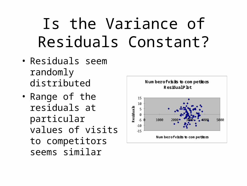
Is the Variance of Residuals Constant?

• Residuals seem randomly distributed

• Range of the residuals at particular values of visits to competitors seems similar

Number of visits to competitors Residual Plot

-15

-10

-5

0

5

10

15

0 1000 2000 3000 4000 5000

Number of visits to competitorsR

esi

du

als

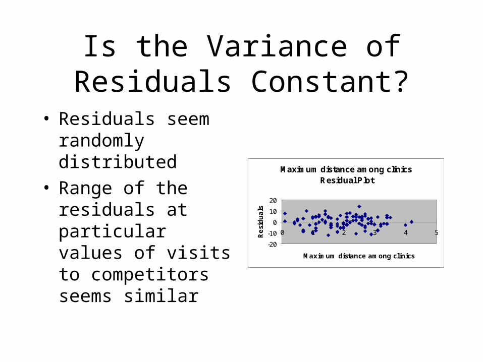
Is the Variance of Residuals Constant?

• Residuals seem randomly distributed

• Range of the residuals at particular values of visits to competitors seems similar

Maximum distance among clinics Residual Plot

-20

-10

0

10

20

0 1 2 3 4 5

Maximum distance among clinicsR

esi

du

als

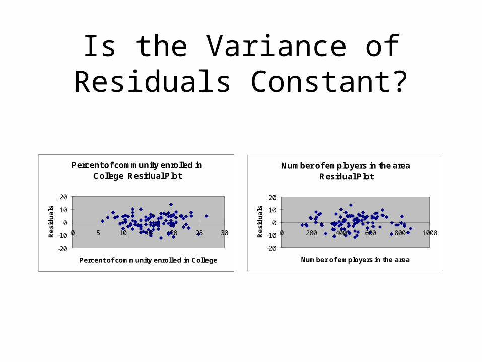
Is the Variance of Residuals Constant?

Percent of community enrolled in College Residual Plot

-20

-10

0

10

20

0 5 10 15 20 25 30

Percent of community enrolled in College

Re

sid

ua

ls

Number of employers in the area Residual Plot

-20

-10

0

10

20

0 200 400 600 800 1000

Number of employers in the areaR

esi

du

als

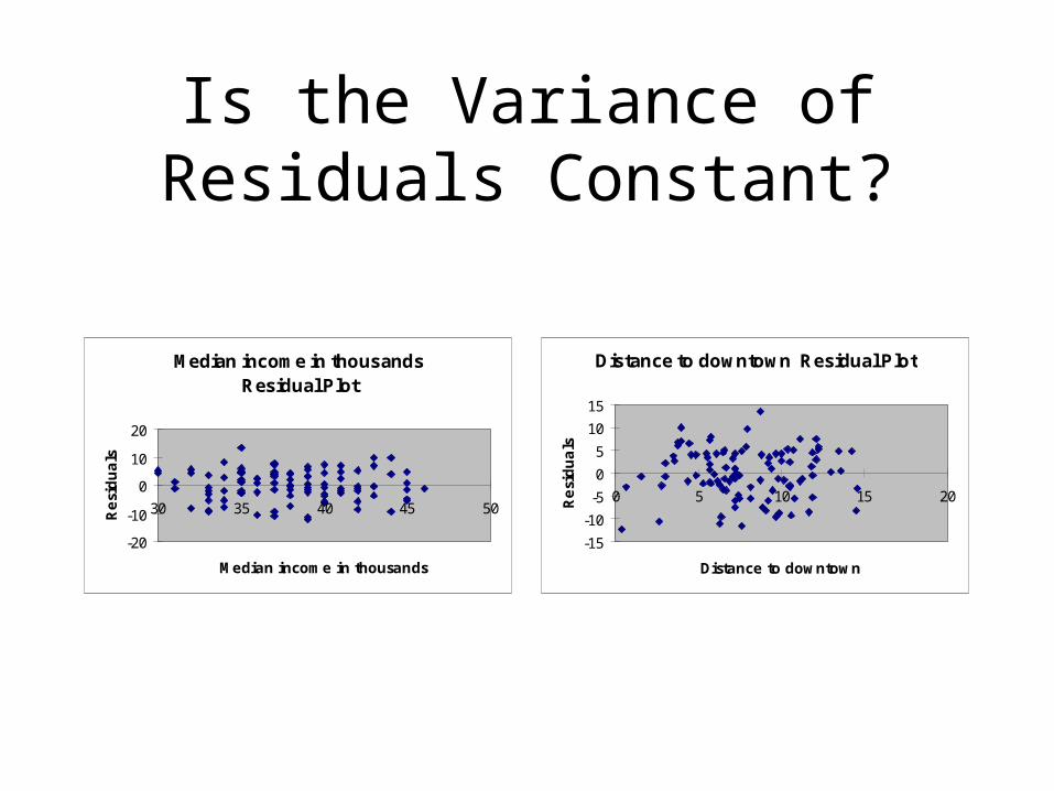
Is the Variance of Residuals Constant?

Median income in thousands Residual Plot

-20

-10

0

10

20

30 35 40 45 50

Median income in thousands

Re

sid

ua

ls

Distance to downtown Residual Plot

-15

-10

-5

0

5

10

15

0 5 10 15 20

Distance to downtownR

esi

du

als

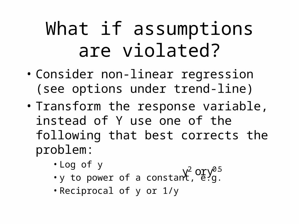
What if assumptions are violated?

• Consider non-linear regression (see options under trend-line)

• Transform the response variable, instead of Y use one of the following that best corrects the problem:

• Log of y

• y to power of a constant, e.g.

• Reciprocal of y or 1/y

y2 or y0.5

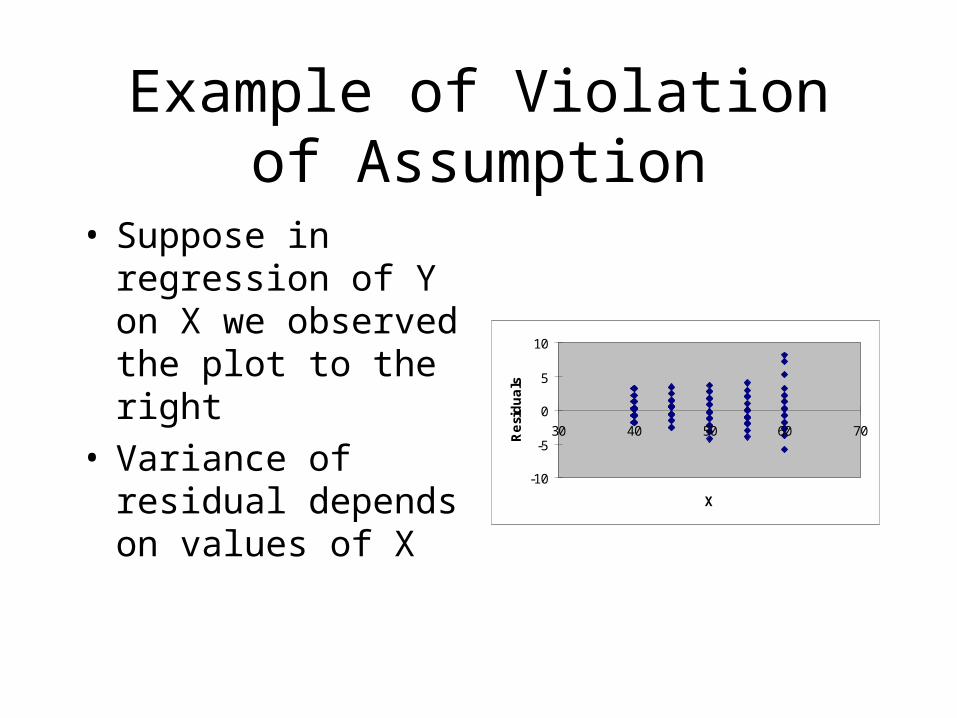
Example of Violation of Assumption

• Suppose in regression of Y on X we observed the plot to the right

• Variance of residual depends on values of X

-10

-5

0

5

10

30 40 50 60 70

XR

esi

du

als

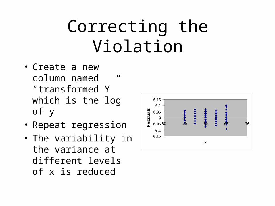
Correcting the Violation

• Create a new column named “transformed Y” which is the log of y

• Repeat regression• The variability in the

variance at different levels of x is reduced

-0.15

-0.1

-0.05

0

0.05

0.1

0.15

30 40 50 60 70

XR

esi

du

als

What to Do If Variables Are Non Linear?

• Use nonlinear regression (see trend line command)• Use Linear regression

Transform the x variable and create a new column of data. Choose transformations based on the shape of the relationship you see in the data

• Use x to power of a constant

• Use log of x

• Use reciprocal of x

Use the transformed column of data in the linear regression

Relationship Among Regression Components

SSE F Assessment

0 0 1 Perfect

Small Small Close to 1

Large Good

Large Large Close to 0

Small Poor

0 0 Useless

Number of observation is shown as n. Number of variables as k. The variation in Y is

(yi-y)2 (yi-y)2/ (n-k-1)

S R2

(yi-y)2

Multicollinearity

Problem in interpretation of regression coefficients when

independent variables are correlated

New Assumption Unique to Multiple

Regression

Sample Problem• Download data• Construct a measure of severity of substance

abuse to predict length of stay of patients in treatment programs. The more the severity the shorter the stay.

• 30 patients were followed and their length of stay as well as their scores on 10 co-morbidities were recorded. Higher score indicates more of the factor is present.

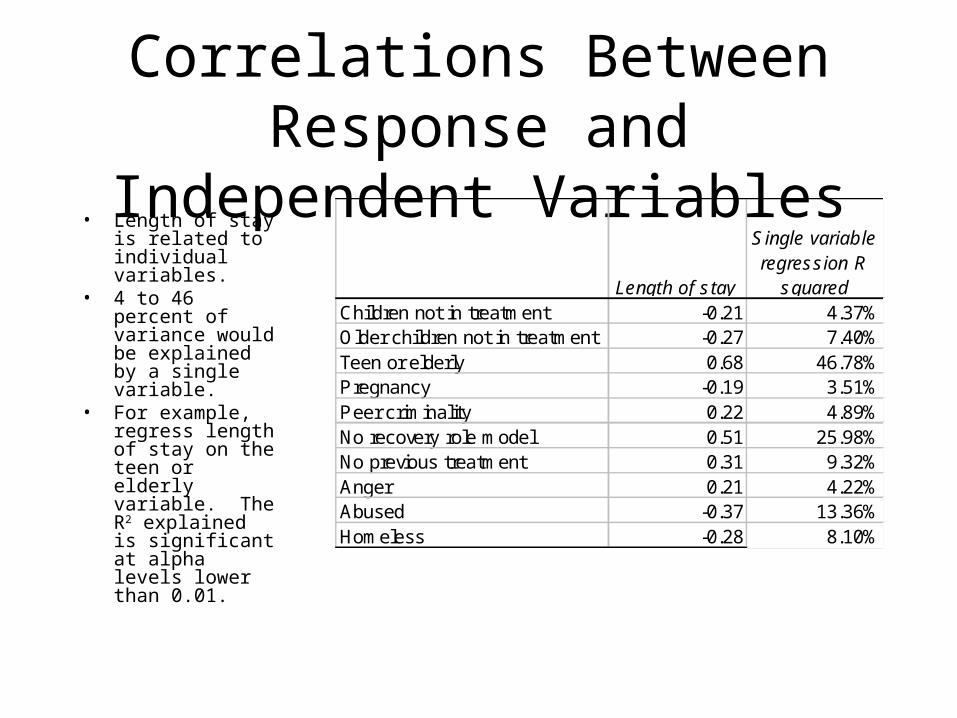
Correlations Between Response and Independent Variables

• Length of stay is related to individual variables.

• 4 to 46 percent of variance would be explained by a single variable.

• For example, regress length of stay on the teen or elderly variable. The R2 explained is significant at alpha levels lower than 0.01.

Length of stay

Single variable regression R

squaredChildren not in treatment -0.21 4.37%Older children not in treatment -0.27 7.40%Teen or elderly 0.68 46.78%Pregnancy -0.19 3.51%Peer criminality 0.22 4.89%No recovery role model 0.51 25.98%No previous treatment 0.31 9.32%Anger 0.21 4.22%Abused -0.37 13.36%Homeless -0.28 8.10%

Multiple Regression

• Note that adjusted R2 measures the percent of variance in Y (length of stay) explained.

• 31% is explained by the linear combination of the variables.

Regression StatisticsMultiple R 0.74R Square 0.55Adjusted R Square 0.31Standard Error 142.36Observations 30.00

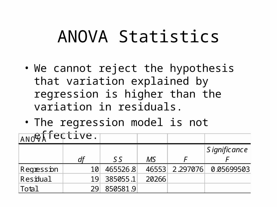
ANOVA Statistics

• We cannot reject the hypothesis that variation explained by regression is higher than the variation in residuals.

• The regression model is not effective.

ANOVA

df SS MS FSignificance

FRegression 10 465526.8 46553 2.297076 0.05699503Residual 19 385055.1 20266Total 29 850581.9

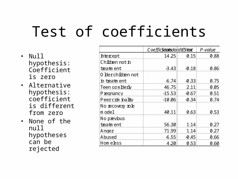
Test of coefficients

• Null hypothesis: Coefficient is zero

• Alternative hypothesis: coefficient is different from zero

• None of the null hypotheses can be rejected

CoefficientsStandard Errort Stat P-valueIntercept 14.25 0.15 0.88Children not in treatment -3.43 -0.18 0.86Older children not in treatment -6.74 -0.33 0.75Teen or elderly 46.75 2.11 0.05Pregnancy -15.53 -0.67 0.51Peer criminality -10.06 -0.34 0.74No recovery role model 40.11 0.63 0.53No previous treatment 56.30 1.14 0.27Anger 71.99 1.14 0.27Abused -6.55 -0.45 0.66Homeless 4.20 0.53 0.60

But if we look at it in single variable regressions …

• Regress length of stay on teen or elderly variable

• Coefficient is statistically significant

Coefficients t Stat P-valueIntercept 95.11 3.26 0.00Teen or elderly 64.59 4.96 0.00

Why would a single variable relationship disappear when

looking at it in a multiple regression?

Explanation of Collinearity

• Collinearity exists when independent variables are correlated

• Collinearity increases sample variability and SSE• Previously significant relationships no longer are

significant when they enter into the equation with other collinear variables

• Conceptually the percent of variance explained by colinear independent variables is shared among the independent variables

Detection of Collinearity

• Exists in almost all situation except when full factorial designs are used to set up the experiment

• The key question is how much collinearity is too much

• A heuristic is that correlations above 0.30 are problematic

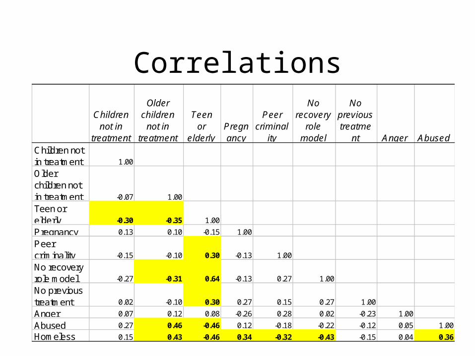
Correlations

Children not in

treatment

Older children

not in treatment

Teen or

elderlyPregnancy

Peer criminal

ity

No recovery

role model

No previous treatme

nt Anger AbusedChildren not in treatment 1.00

Older children not in treatment -0.07 1.00

Teen or elderly -0.30 -0.35 1.00

Pregnancy 0.13 0.10 -0.15 1.00

Peer criminality -0.15 -0.10 0.30 -0.13 1.00

No recovery role model -0.27 -0.31 0.64 -0.13 0.27 1.00

No previous treatment 0.02 -0.10 0.30 0.27 0.15 0.27 1.00

Anger 0.07 0.12 0.08 -0.26 0.28 0.02 -0.23 1.00

Abused 0.27 0.46 -0.46 0.12 -0.18 -0.22 -0.12 0.05 1.00

Homeless 0.15 0.43 -0.46 0.34 -0.32 -0.43 -0.15 0.04 0.36

How to Correct for Collinearity?

• Choose independent variable with low collinearity

• Use stepwise regressionA procedure in which the most correlated variable is entered into the equation first, then remaining variance in Y is explained by the next most correlated variable and so on. In this procedure the order of entry of the variables matter.

Non Interval Independent Variables

• Some time the independent variable is measured on an ordinal or nominal scale e.g., gender

• To use regression assign 0 to absence of the variable and 1 to presence and use this indicator variable in your regression analysis

• If more than two levels use multiple indicator variables one for each level except for the reference level

Example of An Indicator Variable

• Type of clinician includes the following levels: psychiatrist, psychologist, counselor, social worker

• Use 3 indicator variables:Presence of psychiatrist

Presence of psychologist

Presence of counselor

• When all three are not present then it is assumed that the clinician was a social worker

Another Example of An Indicator Variable

• Patients diagnoses may be any of the following levelsNo MI

MI

MI with complications

• Use 2 indicator variables:Presence of MI

Presence of MI with complications

• When both indicators are zero, then diagnoses is no MI

Test for Interactions

• Consider two variables x1 and x2. We had assumed

• Sometimes there are interactions in first order linear models so that we can look at

• Multiply x1 column of data with x2 column of data and put into a separate column

• y = 0 + 1x1 + 2x2 +

y = 0 + 1x1 + 2x2 + 3x1x2 +

Example

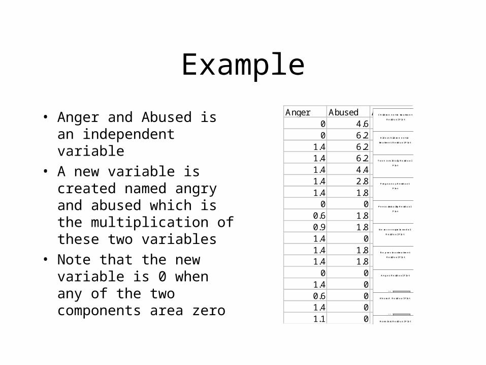
• Anger and Abused is an independent variable

• A new variable is created named angry and abused which is the multiplication of these two variables

• Note that the new variable is 0 when any of the two components area zero

Anger Abused Anger and abused0 4.6 00 6.2 0

1.4 6.2 8.681.4 6.2 8.681.4 4.4 6.161.4 2.8 3.921.4 1.8 2.52

0 0 00.6 1.8 1.080.9 1.8 1.621.4 0 01.4 1.8 2.521.4 1.8 2.52

0 0 01.4 0 00.6 0 01.4 0 01.1 0 0

C h ild re n n o t in tre a tme n t

R e sid u a l P lo t

0

0.2

0.4

0.6

0.8

1

1 .2

0 5

C h i ld re n n o t in

tre a tme n t

O ld e r c h ild re n n o t in

tre a tme n t R e sid u a l P lo t

0

0.2

0.4

0.6

0.8

1

1 .2

0 5

O ld e r c h i ld re n n o t in

tre a tme n t

T e e n o r e ld e rly R e sid u a l

P lo t

0

0.2

0.4

0.6

0.8

1

1 .2

0 5

T e e n o r e ld e rly

P re g n a n c y R e sid u a l

P lo t

0

0.2

0.4

0.6

0.8

1

1 .2

0 5

P re g n a n c y

P e e r c rimin a lity R e sid u a l

P lo t

0

0.2

0.4

0.6

0.8

1

1 .2

0 5

P e e r c rimin a l i ty

No re c o v e ry ro le mo d e l

R e sid u a l P lo t

0

0.2

0.4

0.6

0.8

1

1 .2

0 2

N o re c o v e ry ro le mo d e l

N o p re v io u s tre a tme n t

R e sid u a l P lo t

0

0.2

0.4

0.6

0.8

1

1 .2

0 2

N o p re v i o u s tre a tme n t

A n g e r R e sid u a l P lo t

0

0.2

0.4

0.6

0.8

1

1 .2

0 2

A n g e r

A b u se d R e sid u a l P lo t

0

0.2

0.4

0.6

0.8

1

1 .2

0 1 0

A b u se d

Ho me le ss R e sid u a l P lo t

0

0.2

0.4

0.6

0.8

1

1 .2

0 2

H o me l e ss

Regression with Interaction Terms

• Include the new column in the regression• Not that being abused is not related to length of

stay• Note that being angry and abused is related

Coefficients t Stat P-valueIntercept 64.92 0.77 0.45Anger 186.23 2.22 0.04Abused 8.91 0.37 0.71Anger and abused -41.56 -1.79 0.08

Test for Interactions (Continued)

• Previous example showed interaction term between two variables

• You can include interaction terms between any pair of variables

• But be careful not to have too many variables in the model

• Number of observations should be at least 3-4 times number of variables in a regression equation

Which Interactions to Include?

• Do not go fishing for interaction terms in the data by including all interactions until something significant is found

• Look at the underlying problem and think through if conceptually an interaction term makes sense

Take Home Lesson• Multiple regression is similar to single variable

regression in concept.Similar F test for regression.Similar t test for coefficients.Similar concept of .

• Test the assumptions that residuals have a Normal distribution, constant variance, and are independent.

• Test for collinearity.• Test for interactions. Test if there are non-linear

relationships

R2