Multiple Regression

STATGRAPHICS – Rev. 7/7/2009

2009 by StatPoint Technologies, Inc. Multiple Regression - 1

Multiple Regression Summary The Multiple Regression procedure is designed to construct a statistical model describing the impact of a two or more quantitative factors X on a dependent variable Y. The procedure includes an option to perform a stepwise regression, in which a subset of the X variables is selected. The fitted model may be used to make predictions, including confidence limits and/or prediction limits. Residuals may also be plotted and influential observations identified. The procedure contains additional options for transforming the data using either a Box-Cox or Cochrane-Orcutt transformation. The first option is useful for stabilizing the variability of the data, while the second is useful for handling time series data in which the residuals exhibit serial correlation. Sample StatFolio: multiple reg.sgp Sample Data: The file 93cars.sgd contains information on 26 variables for n = 93 makes and models of automobiles, taken from Lock (1993). The table below shows a partial list of 4 columns from that file: Make Model MPG

Highway Weight Horsepower Wheelbase Drivetrain

Acura Integra 31 2705 140 102 front Acura Legend 25 3560 200 115 front Audi 90 26 3375 172 102 front Audi 100 26 3405 172 106 front BMW 535i 30 3640 208 109 rear Buick Century 31 2880 110 105 front Buick LeSabre 28 3470 170 111 front Buick Roadmaster 25 4105 180 116 rear Buick Riviera 27 3495 170 108 front Cadillac DeVille 25 3620 200 114 front Cadillac Seville 25 3935 295 111 front Chevrolet Cavalier 36 2490 110 101 front

A model is desired that can predict MPG Highway from Weight, Horsepower, Wheelbase, and Drivetrain.



Data Input The data input dialog box requests the names of the columns containing the dependent variable Y and the independent variables X:

Y: numeric column containing the n observations for the dependent variable Y. X: numeric columns containing the n values for the independent variables X. Either column

names or STATGRAPHICS expressions may be entered. Select: subset selection. Weight: an optional numeric column containing weights to be applied to the squared

residuals when performing a weighted least squares fit. In the example, note the use of the expression Weight^2 to add a second-order term involving the weight of the vehicle. This was added after examining an X-Y plot that showed significant curvature with respect to Weight. The categorical factor Drivetrain has also be introduced into the model through the Boolean expression Drivetrain=”front”, which sets up an indicator variable that takes the value 1 if true and 0 if false. The model to be fit thus takes the form:

MPG Highway = 0 + 1Weight + 2Weight2 + 3Horsepower + 4Wheelbase + 5X5 (1)

where



0

15X if (2)

rearDrivetrain

frontDrivetrain

Analysis Summary The Analysis Summary shows information about the fitted model. Multiple Regression - MPG Highway Dependent variable: MPG Highway Standard T Parameter Estimate Error Statistic P-Value CONSTANT 49.8458 10.5262 4.73539 0.0000 Weight -0.0273685 0.00530942 -5.1547 0.0000 Weight^2 0.00000261405 8.383E-7 3.11827 0.0025 Horsepower 0.0145764 0.009668 1.50769 0.1353 Wheelbase 0.338687 0.103479 3.273 0.0015 Drive Train="front" 0.632343 0.73879 0.855918 0.3944

Analysis of Variance Source Sum of Squares Df Mean Square F-Ratio P-Value Model 1902.18 5 380.435 46.41 0.0000 Residual 713.136 87 8.19696 Total (Corr.) 2615.31 92

R-squared = 72.7323 percent R-squared (adjusted for d.f.) = 71.1652 percent Standard Error of Est. = 2.86303 Mean absolute error = 2.13575 Durbin-Watson statistic = 1.685 (P=0.0601) Lag 1 residual autocorrelation = 0.156111

Included in the output are: Variables: identification of the dependent variable. The general form of the model is

Y = 0 + 1X1 + 2X2 + … + kXk (3)

where k is the number of independent variables.

Coefficients: the estimated coefficients, standard errors, t-statistics, and P values. The estimates of the model coefficients can be used to write the fitted equation, which in the example is

MPG Highway = 49.8458 - 0.0273685*Weight + 0.00000261405*Weight2

+ 0.0145764*Horsepower + 0.338687*Wheelbase + 0.632343*Drive Train="front" (4)

The t-statistic tests the null hypothesis that the corresponding model parameter equals 0, based on the Type 3 sums of squares (the extra sums of squares attributable to each variable if it is entered into the model last). Large P-Values (greater than or equal to 0.05 if operating at the 5% significance level) indicate that a term can be dropped without significantly degrading the model provided all of the other variables remain in the model. In the current



case, both Horsepower and Drivetrain are not significant. Thus, either variable (but not necessarily both) could be dropped from the model without hurting its predictive power significantly.

Analysis of Variance: decomposition of the variability of the dependent variable Y into a

model sum of squares and a residual or error sum of squares. Of particular interest is the F-test and its associated P-value, which tests the statistical significance of the fitted model. A small P-Value (less than 0.05 if operating at the 5% significance level) indicates that a significant relationship of the form specified exists between Y and the independent variables. In the sample data, the model is highly significant.

Statistics: summary statistics for the fitted model, including:

R-squared - represents the percentage of the variability in Y which has been explained by the fitted regression model, ranging from 0% to 100%. For the sample data, the regression has accounted for about 72.7% of the variability in the miles per gallon. The remaining 27.3% is attributable to deviations from the model, which may be due to other factors, to measurement error, or to a failure of the current model to fit the data adequately.

Adjusted R-Squared – the R-squared statistic, adjusted for the number of coefficients in the model. This value is often used to compare models with different numbers of coefficients. Standard Error of Est. – the estimated standard deviation of the residuals (the deviations around the model). This value is used to create prediction limits for new observations. Mean Absolute Error – the average absolute value of the residuals. Durbin-Watson Statistic – a measure of serial correlation in the residuals. If the residuals vary randomly, this value should be close to 2. A small P-value indicates a non-random pattern in the residuals. For data recorded over time, a small P-value could indicate that some trend over time has not been accounted for. In the current example, the P-value is greater than 0.05, so there is not a significant correlation at the 5% significance level. Lag 1 Residual Autocorrelation – the estimated correlation between consecutive residuals, on a scale of –1 to 1. Values far from 0 indicate that significant structure remains unaccounted for by the model.



Analysis Options

Fitting Procedure – specifies the method used to fit the regression model. The options are:

o Ordinary Least Squares – fits a model using all of the independent variables. o Forward Stepwise Selection – performs a forward stepwise regression. Beginning with

a model that includes only a constant, the procedure brings in variables one at a time provided that they will be statistically significant once added. Variables may also be removed at later steps if they are no longer statistically significant.

o Backward Stepwise Selection – performs a backward stepwise regression. Beginning

with a model that includes all variables, the procedure removes variables one at a time if they are not statistically significant. Removed variables may also be added to the model at later steps if they become statistically significant.

o Box-Cox Optimization – fits a model involving all of the independent variables. The

dependent variable, however, is modified by raising it to a power. The method of Box and Cox is used to determine the optimum power. Box-Cox transformations are a way of dealing with situations in which the deviations from the regression model do not have a constant variance.

o Cochrane-Orcutt Optimization – fits a model involving all of the independent

variables. However, the least squares procedure is modified to allow for autocorrelation between successive residuals. The value of the lag 1 autocorrelation coefficient is determined using the method of Cochrane and Orcutt. The Cochrane-Orcutt transformation is a method for dealing with situations in which the model residuals are not independent.



Constant in model – If this option is not checked, the constant term 0 will be omitted from

the model. Removing the constant term allows for regression through the origin. Power – Specifies the power to which the dependent variable is raised. The default value of

1.0 implies no power transformation. Addend – Specifies an amount that is added to the dependent variable before it is raised to

the specified power. Autocorrelation – Specifies the lag 1 autocorrelation of the residuals. The default value of

0.0 implies that the residuals are assumed to be independent. If the Cochrane-Orcutt procedure is used, this value provides the starting value for the procedure.

Selection Criterion – If performing a forward or backward stepwise regression, this

specifies whether variable entry and removal should be based on the F-ratio or its associated P-value.

= F-to-Enter - In a stepwise regression, variables will be entered into the model at a given step

if their F values are greater than or equal to the F-to-Enter value specified. F-to-Remove - In a stepwise regression, variables will be removed from the model at a given

step if their F values are less than the F-to-Remove value specified. P-to-Enter - In a stepwise regression, variables will be entered into the model at a given step

if their P values are less than or equal to the P-to-Enter value specified. P-to-Remove - In a stepwise regression, variables will be removed from the model at a given

step if their P values are greater than the P-to-Remove value specified. Max Steps – maximum number of steps permitted when doing a stepwise regression. Display – whether to display the results at each step when doing a stepwise regression. Example – Stepwise Regression The model fit to the automobile data showed 2 insignificant variables. To remove them from the model, Analysis Options may be used to perform either a forward stepwise selection or a backward stepwise selection.

Forward selection – Begins with a model involving only a constant term and enters one variable at a time based on its statistical significance if added to the current model. At each step, the algorithm brings into the model the variable that will be the most statistically significant if entered. Selection of variables is based on either an F-to-enter test or a P-to-enter test In the former case, as long as the most significant variable has an F value greater or equal to that specified on the Analysis Summary dialog box, it will be brought into the model. When no variable has a large enough F value, variable selection stops. In addition, variables brought into the model early in



the procedure may be removed later if their F value falls below the F-to-remove criterion.

Backward selection – Begins with a model involving all the variables specified on the data input dialog box and removes one variable at a time based on its statistical significance in the current model. At each step, the algorithm removes from the model the variable that is the least statistically significant. Removal of variables is based on either an F-to-remove test or a P-to-enter test. In the former case, if the least significant variable has an F value less than that specified on the Analysis Summary dialog box, it will be removed from the model. When all remaining variables have large F values, the procedure stops. In addition, variables removed from the model early in the procedure may be re-entered later if their F values reach the F-to-enter criterion.

In the current example, a backwards selection procedure yields the following:

Stepwise regression Method: backward selection F-to-enter: 4.0 F-to-remove: 4.0 Step 0: 5 variables in the model. 87 d.f. for error. R-squared = 72.73% Adjusted R-squared = 71.17% MSE = 8.19696 Step 1: Removing variable Drive Train="front" with F-to-remove =0.732595 4 variables in the model. 88 d.f. for error. R-squared = 72.50% Adjusted R-squared = 71.25% MSE = 8.17206 Step 2: Removing variable Horsepower with F-to-remove =2.22011 3 variables in the model. 89 d.f. for error. R-squared = 71.81% Adjusted R-squared = 70.86% MSE = 8.28409 Final model selected.

In the first step, Drivetrain is removed since it is the least significant. At the second step, Horsepower is removed. The algorithm then stops, since all remaining variables have F-to-remove values greater than 4, and all previously removed variables have F-to-enter values less than 4. The reduced model is summarized below: Multiple Regression - MPG Highway Dependent variable: MPG Highway Independent variables: Weight Weight^2 Horsepower Wheelbase Drive Train="front" Standard T Parameter Estimate Error Statistic P-Value CONSTANT 51.8628 10.2179 5.07569 0.0000 Weight -0.0245435 0.00506191 -4.84867 0.0000 Weight^2 0.00000236841 8.25606E-7 2.86869 0.0051 Wheelbase 0.28345 0.0899993 3.14947 0.0022





NOTE: from here forward in this document, the results will be based on the reduced model without Drivetrain or Wheelbase. Example – Box-Cox Transformation If it is suspected that the variability of Y changes as its level changes, it is useful to consider performing a transformation on Y. The Box-Cox transformations are of the general form

1

2 YY (5)

in which the data is raised to a power 1 after shifting it a certain amount 2. Often, the shift parameter 2 is set equal to 0. This class includes square roots, logarithms, reciprocals, and other common transformations, depending on the power. Examples include:

Power Transformation Description = 2 2YY square = 1 YY untransformed data = 0.5 YY square root

= 0.333 3 YY cube root

= 0 )ln(YY logarithm

= -0.5

YY

1

inverse square root

= -1Y

Y1

reciprocal

Using Analysis Options, you can specify the values for 1 or 2, or specify just 2 and have the program find an optimal value for 1 using the methods proposed by Box and Cox (1964). For the sample data, a plot of the residuals versus predicted values does show some change in variability as the predicted value changes:



Residual Plot

20 25 30 35 40 45 50

predicted MPG Highway

-3.7

-1.7

0.3

2.3

4.3

Stu

dent

ized

res

idua

l

The smaller cars tend to be somewhat more variable than the larger cars. Asking the program to optimize the Box-Cox transformation yields: Multiple Regression - MPG Highway Dependent variable: MPG Highway Independent variables: Weight Weight^2 Wheelbase Box-Cox transformation applied: power = -0.440625 shift = 0.0 Standard T Parameter Estimate Error Statistic P-Value CONSTANT 230.703 9.37335 24.6126 0.0000 Weight -0.0129299 0.00464353 -2.78451 0.0065 Weight^2 6.18885E-7 7.57367E-7 0.817153 0.4160 Wheelbase 0.229684 0.0825606 2.782 0.0066



Apparently, an inverse square root of MPG Highway improves the properties of the residuals, as illustrated in the new residual plot:



Residual Plot


Stu

dent

ized

res

idua

l

20 25 30 35 40 45 50-3.6

-1.6

0.4

2.4

4.4

Note: some caution is necessary here, however, since the transformation may be heavily influenced by one or two outliers. To simplify the discussion that follows, however, the rest of this document will work with the untransformed model.

Component Effects Plot Plotting a multiple regression model is not as easy as plotting a simple regression model, since the space of the X variables is multi-dimensional. One useful way to illustrate the results is through the Component Effects Plot, which plots of the portion of the fitted regression model corresponding to any single variable.

Component+Residual Plot for MPG Highway

Wheelbase

com

pone

nt e

ffec

t

90 95 100 105 110 115 120-12

-8

-4

0

4

8

12

The line on the plot is defined by

jjj xx (6)

where is the estimated regression coefficient for variable j, xj represents the value of variable

j as plotted on the horizontal axis, and j

jx is the average value of the selected independent

variable amongst the n observations used to fit the model. You can judge the importance of a factor by noting how much the component effect changes over the range of the selected variable.



For example, as Wheelbase changes from 90 to 120, the component effect changes from about –4 to +4. This implies that differences in Wheelbase account for a swing of about 8 miles per gallon. The points on the above plot represent each of the n = 93 automobiles in the dataset. The vertical positions are equal to the component effect plus the residual from the fitted model. This allows you to gage the relative importance of a factor compared to the residuals. In the above plot, some of the residuals are as large if not larger than the effect of Wheelbase, indicating that other important factors may be missing from the model. Pane Options

Plot versus: the factor used to define the component effect.

Conditional Sums of Squares The Conditional Sums of Squares pane displays a table showing the statistical significance of each coefficient in the model as it added to the fit:

Further ANOVA for Variables in the Order Fitted Source Sum of Squares Df Mean Square F-Ratio P-Value Weight 1718.7 1 1718.7 207.47 0.0000 Weight^2 77.1615 1 77.1615 9.31 0.0030 Wheelbase 82.1713 1 82.1713 9.92 0.0022 Model 1878.03 3

The table decomposes the model sum of squares SSR into contributions due to each coefficient by showing the increase in SSR as each term is added to the model. These sums of squares are often called Type I sums of squares. The F-Ratios compare the mean square for each term to the MSE of the fitted model. These sums of squares are useful when fitting polynomial models, as discussed in the Polynomial Regression documentation. In the above table, all variables are statistically significant at the 1% significance level since their P-Values are well below 0.01.



Observed versus Predicted The Observed versus Predicted plot shows the observed values of Y on the vertical axis and the

predicted values Y on the horizontal axis.

Plot of MPG Highway

20 25 30 35 40 45 50

predicted

20

25

30

35

40

45

50

obse

rved

If the model fits well, the points should be randomly scattered around the diagonal line. Any change in variability from low values of Y to high values of Y might indicate the need to transform the dependent variable before fitting a model to the data. In the above plot, the variability appears to increase somewhat as the predicted values get large.

Residual Plots As with all statistical models, it is good practice to examine the residuals. In a regression, the residuals are defined by (7) iii yye ˆ i.e., the residuals are the differences between the observed data values and the fitted model. The Multiple Regression procedure creates 3 residual plots:

1. versus X.

2. versus predicted value Y . 3. versus row number.



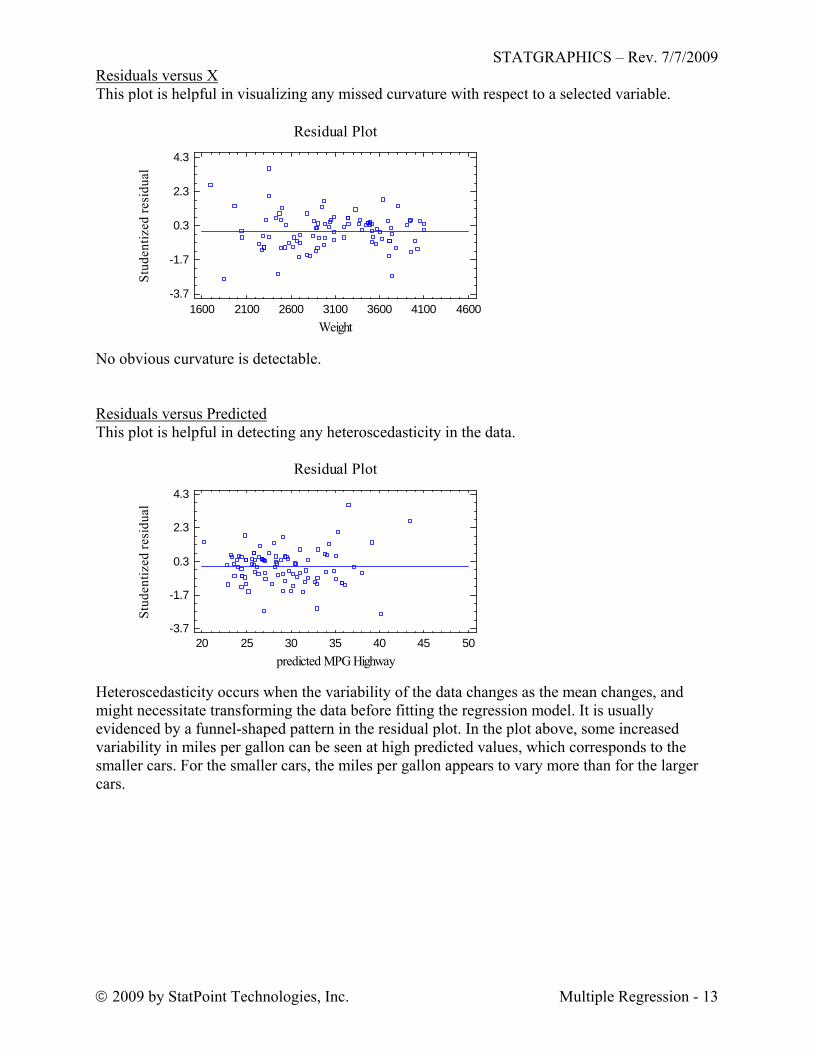
Residuals versus X This plot is helpful in visualizing any missed curvature with respect to a selected variable.

Residual Plot

Weight

Stu

dent

ized

res

idua

l

1600 2100 2600 3100 3600 4100 4600-3.7

-1.7

0.3

2.3

4.3

No obvious curvature is detectable. Residuals versus Predicted This plot is helpful in detecting any heteroscedasticity in the data.

Residual Plot


Stu

dent

ized

res

idua

l

20 25 30 35 40 45 50-3.7

-1.7

0.3

2.3

4.3

Heteroscedasticity occurs when the variability of the data changes as the mean changes, and might necessitate transforming the data before fitting the regression model. It is usually evidenced by a funnel-shaped pattern in the residual plot. In the plot above, some increased variability in miles per gallon can be seen at high predicted values, which corresponds to the smaller cars. For the smaller cars, the miles per gallon appears to vary more than for the larger cars.



Residuals versus Observation This plot shows the residuals versus row number in the datasheet:

Residual Plot

0 20 40 60 80 100

row number

-3.7

-1.7

0.3

2.3

4.3S

tude

ntiz

ed re

sidu

al

If the data are arranged in chronological order, any pattern in the data might indicate an outside influence. In the above plot, no obvious trend is present, although there is a standardized residual in excess of 3.5, indicating that it is more than 3.5 standard deviations from the fitted curve. Pane Options

Plot: The following residuals may be plotted on each residual plot:

1. Residuals – the residuals from the least squares fit. 2. Studentized residuals – the difference between the observed values yi and the predicted

values iy when the model is fit using all observations except the i-th, divided by the

estimated standard error. These residuals are sometimes called externally deleted residuals, since they measure how far each value is from the fitted model when that model is fit using all of the data except the point being considered. This is important, since a large outlier might otherwise affect the model so much that it would not appear to be unusually far away from the line.

Plot versus: the independent variable to plot on the horizontal axis, if relevant.



Unusual Residuals Once the model has been fit, it is useful to study the residuals to determine whether any outliers exist that should be removed from the data. The Unusual Residuals pane lists all observations that have Studentized residuals of 2.0 or greater in absolute value.

Unusual Residuals Predicted Studentized Row Y Y Residual Residual 31 33.0 40.1526 -7.15265 -2.81 36 20.0 26.9631 -6.96309 -2.62 39 50.0 43.4269 6.5731 2.72 42 46.0 36.4604 9.53958 3.66 60 26.0 32.8753 -6.8753 -2.50 73 41.0 35.3266 5.67338 2.04

Studentized residuals greater than 3 in absolute value correspond to points more than 3 standard deviations from the fitted model, which is a very rare event for a normal distribution. In the sample data, row #42 is more 3.5 standard deviations out. Row #42 is a Honda Civic, which was listed in the dataset as achieving 46 miles per gallon, while the model predicts less than 37. Points can be removed from the fit while examining any of the residual plots by clicking on a point and then pressing the Exclude/Include button on the analysis toolbar.

Influential Points In fitting a regression model, all observations do not have an equal influence on the parameter estimates in the fitted model. Those with unusual values of the independent variables tend to have more influence than the others. The Influential Points pane displays any observations that have high influence on the fitted model:

Influential Points Mahalanobis Row Leverage Distance DFITS 19 0.139122 13.5555 0.18502 28 0.246158 28.3994 0.685044 31 0.156066 15.6544 -1.225 36 0.0961585 8.58597 -0.849931 39 0.250016 29.0136 1.89821 60 0.0298891 1.78389 -0.463748 73 0.0352144 2.29596 0.451735 83 0.102406 9.27903 0.573505

Average leverage of single data point = 0.0434783 Points are placed on this list for one of the following reasons: Leverage – measures how distant an observation is from the mean of all n observations in

the space of the independent variables. The higher the leverage, the greater the impact of the point on the fitted values .y Points are placed on the list if their leverage is more than 3 times that of an average data point.

Mahalanobis Distance – measures the distance of a point from the center of the collection of

points in the multivariate space of the independent variables. Since this distance is related to leverage, it is not used to select points for the table.



DFITS – measures the difference between the predicted values iy when the model is fit with

and without the i-th data point. Points are placed on the list if the absolute value of DFITS

exceeds np /2 , where p is the number of coefficients in the fitted model. In the sample data, rows #28 and #39 show a leverage value of nearly 6 times that of an average data point. Rows #31 and #39 have the largest values of DFITS. Removing high influence points is not recommended on a routine basis. However, it is important to be aware of their impact on the estimated model.

Confidence Intervals The Confidence Intervals pane shows the potential estimation error associated with each coefficient in the model.

95.0% confidence intervals for coefficient estimates Standard Parameter Estimate Error Lower Limit Upper Limit CONSTANT 55.0336 9.61121 35.9333 74.1339 Weight -0.023276 0.00475462 -0.0327248 -0.0138271 Weight^2 0.00000230174 7.73643E-7 7.64284E-7 0.0000038392 Wheelbase 0.220693 0.0860352 0.0497156 0.39167

Pane Options

Confidence Level: percentage level for the confidence intervals.

Correlation Matrix The Correlation Matrix displays estimates of the correlation between the estimated coefficients.

Correlation matrix for coefficient estimates CONSTANT Weight Weight^2 Wheelbase CONSTANT 1.0000 -0.6247 0.7456 -0.6847 Weight -0.6247 1.0000 -0.9776 -0.1349 Weight^2 0.7456 -0.9776 1.0000 -0.0508 Wheelbase -0.6847 -0.1349 -0.0508 1.0000

This table can be helpful in determining how well the effects of different independent variables have been separated from each other. Note the high correlation between the coefficients of Weight and Weight2. This is normal whenever fitting a non-centered polynomial and simply means that the coefficients could change dramatically if a different order polynomial was



selected. The fact that the correlation between the coefficients of Weight and Wheelbase is small is more interesting, since it implies that there is little confounding between the estimated effects of those variables. Confounding or intermixing of the effects of two variables is a common problem when attempting to interpret models estimated from data that was not collected from a designed experiment.

Reports The Reports pane creates predictions using the fitted least squares model. By default, the table includes a line for each row in the datasheet that has complete information on the X variables and a missing value for the Y variable. This allows you to add rows to the bottom of the datasheet corresponding to levels at which you want predictions without affecting the fitted model. For example, suppose a prediction is desired for a car with a Weight of 3500 and a Wheelbase of 105. In row #94 of the datasheet, these values would be added but the MPG Highway column would be left blank. The resulting table is shown below:

Regression Results for MPG Highway Fitted Stnd. Error Lower 95.0% Upper 95.0% Lower 95.0% Upper 95.0% Row Value CL for Forecast CL for Forecast CL for Forecast CL for Mean CL for Mean 94 24.7357 2.91778 18.9381 30.5333 23.7842 25.6872

Included in the table are:

Row - the row number in the datasheet.

Fitted Value - the predicted value of the dependent variable using the fitted model.

Standard Error for Forecast - the estimated standard error for predicting a single new observation.

Confidence Limits for Forecast - prediction limits for new observations at the selected

level of confidence.

Confidence Limits for Mean - confidence limits for the mean value of Y at the selected level of confidence.

For row #94, the predicted miles per gallon is 24.7. Models with those features can be expected to achieve between 18.9 and 30.5 miles per gallon in highway driving. Using Pane Options, additional information about the predicted values and residuals for the data used to fit the model can also be included in the table.



Pane Options

You may include: Observed Y – the observed values of the dependent variable. Fitted Y – the predicted values from the fitted model. Residuals – the ordinary residuals (observed minus predicted). Studentized Residuals – the Studentized deleted residuals as described earlier. Standard Errors for Forecasts – the standard errors for new observations at values of the

independent variables corresponding to each row of the datasheet. Confidence Limits for Individual Forecasts – confidence intervals for new observations. Confidence Limits for Forecast Means – confidence intervals for the mean value of Y at

values of the independent variables corresponding to each row of the datasheet.

Interval Plots The Intervals Plots pane can create a number of interesting types of plots. The plot below shows how precisely the miles per gallon of an automobile can be predicted.

Plot of MPG Highway with Predicted Values

predicted value

MP

G H

ighw

ay

20 25 30 35 40 45 5015

20

25

30

35

40

45

50



An interval is drawn on the plot for each observation in the dataset, showing the 95% prediction limits for a new observation at the corresponding predicted value. Pane Options

Plot Limits For: type of limits to be included. Predicted Values plots prediction limits at

settings of the independent variables corresponding to each of the n observations used to fit the model. Means plots confidence limits for the mean value of Y corresponding to each of the n observations. Forecasts plots prediction limits for rows of the datasheet that have missing values for Y. Forecast Means plots confidence limits for the mean value of Y corresponding to each row in the datasheet with a missing value for Y.

Plot Versus: the value to plot on the horizontal axis. Confidence Level: the confidence percentage used for the intervals.



Autocorrelated Data When regression models are used to fit data that is recorded over time, the deviations from the fitted model are often not independent. This can lead to inefficient estimates of the underlying regression model coefficients and P-values that overstate the statistical significance of the fitted model. As an illustration, consider the following data from Neter et al. (1996), contained in the file company.sgd:

Year and quarter Company Sales ($ millions)

Industry Sales ($ millions)

1983: Q1 20.96 127.3 1983: Q2 21.40 130.0 1983: Q3 21.96 132.7 1983: Q4 21.52 129.4 1984: Q1 22.39 135.0 1984: Q2 22.76 137.1 1984: Q3 23.48 141.2 1984: Q4 23.66 142.8 1985: Q1 24.10 145.5 1985: Q2 24.01 145.3 1985: Q3 24.54 148.3 1985: Q4 24.30 146.4 1986: Q1 25.00 150.2 1986: Q2 25.64 153.1 1986: Q3 26.36 157.3 1986: Q4 26.98 160.7 1987: Q1 27.52 164.2 1987: Q2 27.78 165.6 1987: Q3 28.24 168.7 1987: Q4 28.78 171.7

Regressing company sales against industry sales resulting in a very good linear fit, with a very high R-squared:



Multiple Regression - company sales Dependent variable: company sales Independent variables: industry sales Standard T Parameter Estimate Error Statistic P-Value CONSTANT -1.45475 0.214146 -6.79326 0.0000 industry sales 0.176283 0.00144474 122.017 0.0000



However, the Durbin-Watson statistic is very significant, and the estimated lag 1 residual autocorrelation equals 0.626. A plot of the residuals versus row number shows marked swings around zero:

Residual Plot

0 4 8 12 16 20

row number

-2.3

-1.3

-0.3

0.7

1.7

2.7

Stu

dent

ized

res

idua

l

Clearly, the residuals are not randomly distributed around the regression line. To account for the autocorrelations of the deviations from the regression line, a more complicated error structure can be assumed. A logical extension of the random error model is to let the errors have a first-order autoregressive structure, in which the deviation at time t is dependent upon the deviation at time t-1 in the following manner:

ttt xy 10 (8)

ttt u 1 (9)



where || < 1 and ut are independent samples from a normal distribution with mean 0 and standard deviation . In such a case, transforming both the dependent variable and independent variable according to

1 ttt yyy (10)

1 ttt xxx (11)

leads to the model

ttt uxy 10 1 (12)

which is a linear regression with random error terms. The Analysis Options dialog box allows you to fit a model of the above form using the Cochrane-Orcutt procedure:

You may either specify the value of in the Autocorrelation field and select Ordinary Least Squares, or select Cochrane-Orcutt Optimization and let the value of will be determined iteratively using the specified value as a starting point. In the latter case, the following procedure is used:

Step 1: The model is fit using transformed values of the variables based on the initial value of . Step 2: The value of is re-estimated using the values of t obtained from the fit in Step 1.



Step 3: Steps 1 and 2 are repeated between 4 and 25 times until the change in the derived value of compared to the previous step is less than 0.01.

The results are summarized below using the sample data: Multiple Regression - company sales Dependent variable: company sales Independent variables: industry sales Cochrane-Orcutt transformation applied: autocorrelation = 0.765941 Standard T Parameter Estimate Error Statistic P-Value CONSTANT -0.64188 0.642688 -0.998744 0.3319 industry sales 0.171085 0.00408958 41.8343 0.0000


R-squared = 99.038 percent R-squared (adjusted for d.f.) = 98.9814 percent Standard Error of Est. = 0.0665133 Mean absolute error = 0.0531731 Durbin-Watson statistic = 1.7354 Lag 1 residual autocorrelation = 0.0990169

The above output shows that, at the final value of = 0.766, the Durbin-Watson statistic and the lag 1 residual autocorrelation, computed using the residuals from the regression involving the transformed variables, are much more in line with that expected if the errors are random. The model also changed somewhat.

Save Results The following results may be saved to the datasheet:

1. Predicted Values – the predicted value of Y corresponding to each of the n observations. 2. Standard Errors of Predictions – the standard errors for the n predicted values. 3. Lower Limits for Predictions – the lower prediction limits for each predicted value. 4. Upper Limits for Predictions – the upper prediction limits for each predicted value. 5. Standard Errors of Means – the standard errors for the mean value of Y at each of the n

values of X. 6. Lower Limits for Forecast Means – the lower confidence limits for the mean value of Y

at each of the n values of X. 7. Upper Limits for Forecast Means– the upper confidence limits for the mean value of Y at

each of the n values of X. 8. Residuals – the n residuals. 9. Studentized Residuals – the n Studentized residuals. 10. Leverages – the leverage values corresponding to the n values of X. 11. DFITS Statistics – the value of the DFITS statistic corresponding to the n values of X. 12. Mahalanobis Distances – the Mahalanobis distance corresponding to the n values of X.



Calculations Regression Model

kk XXXY ...22110 (13)

Error Sum of Squares

Unweighted: (14) 2

12210

ˆ...ˆˆˆ

n

ikkii xxxySSE

Weighted: (15) 2

12210

ˆ...ˆˆˆ

n

ikkiii xxxywSSE

Coefficient Estimates

WYXWXX 1 (16)

12 ˆ WXXMSEs (17)

pn

SSEMSE

(18)

where is a column vector containing the estimated regression coefficients, X is an (n, p) matrix containing a 1 in the first column (if the model contains a constant term) and the settings of the k predictor variables in the other columns, Y is a column vector with the values of the dependent variable, and W is an (n, n) diagonal matrix containing the weights wi on the diagonal for a weighted regression or 1’s on the diagonal if weights are not specified. A modified sweep algorithm is used to solve the equations after centering and rescaling of the independent variables.



Analysis of Variance With constant term: Source Sum of Squares Df Mean

Square F-Ratio

Model

n

ii

n

iii

w

yw

WYXbSSR

1

2

1

k k

SSRMSR

MSE

MSRF

Residual

WYXbWYYSSE

n-k-1 1

kn

SSEMSE

Total (corr.)

2

1

n

iii yywSSTO

n-1

Without constant term: Source Sum of Squares Df Mean

Square F-Ratio

Model

WYXbSSR

k k

SSRMSR

MSE

MSRF

Residual

WYXbWYYSSE

n-k kn

SSEMSE

Total

WYYSSTO

n

R-Squared

%1002

SSESSR

SSRR (19)

Adjusted R-Squared

%1

11002

SSESSR

SSE

pn

nRadj (20)



Stnd.Error of Est.

MSE (21) Residuals

kkoii xxye ˆ...ˆˆ11 (22)

Mean Absolute Error

n

ii

n

iii

w

ewMAE

1

1 (23)

Durbin-Watson Statistic

n

ii

n

iii

e

eeD

1

2

2

21

(24)

If n > 500, then

n

DD

/4

2* (25)

is compared to a standard normal distribution. For 100 < n ≤ 500, D/4 is compared to a beta distribution with parameters

2

1

n (26)

For smaller sample sizes, D/4 is compared to a beta distribution with parameters which are based on the trace of certain matrices related to the X matrix, as described by Durbin and Watson (1951) in section 4 of their classic paper. Lag 1 Residual Autocorrelation

n

ii

n

iii

e

eer

1

2

21

1 (27)



Leverage

iiii wXWXXXdiagh 1 (28)

n

ph (29)

Studentized Residuals

ii

iii

hMSE

wed

1 (30)

Mahalanobis Distance

1

)2(

1

/1

n

nn

h

wwhMD

i

n

iiii

i (31)

DFITS

i

i

i

ii h

h

w

dDFITS

1 (32)

Standard Error for Forecast

hhnewh XWXXXMSEYs 1)( 1 (33)

Confidence Limit for Forecast

)(,2/ˆ

newhpnh YstY

(34)

Confidence Limit for Mean

hhpnh XWXXXMSEtY 1,2/

ˆ (35)

Multiple Regression

Data & Analytics

Transcript of Multiple Regression