Multiple moving objects tracking based on random finite sets and … · 2018-02-06 · faculty of...
157
FACULTY OF ELECTRICAL ENGINEERING AND COMPUTING Josip ´ Cesi´ c MULTIPLE MOVING OBJECTS TRACKING BASED ON RANDOM FINITE SETS AND LIE GROUPS DOCTORAL THESIS Zagreb, 2017
Transcript of Multiple moving objects tracking based on random finite sets and … · 2018-02-06 · faculty of...
FACULTY OF ELECTRICAL ENGINEERING AND COMPUTING
Josip Cesic
MULTIPLE MOVING OBJECTS TRACKINGBASED ON RANDOM FINITE SETS AND
LIE GROUPS
DOCTORAL THESIS
Zagreb, 2017

FACULTY OF ELECTRICAL ENGINEERING AND COMPUTING
Josip Cesic
MULTIPLE MOVING OBJECTS TRACKINGBASED ON RANDOM FINITE SETS AND
LIE GROUPS
DOCTORAL THESIS
Supervisor: Professor Ivan Petrovic, PhD
Zagreb, 2017

FAKULTET ELEKTROTEHNIKE I RACUNARSTVA
Josip Cesic
PRACENJE VIŠE GIBAJUCIH OBJEKATAZASNOVANO NA SLUCAJNIM KONACNIM
SKUPOVIMA I LIEVIM GRUPAMA
DOKTORSKI RAD
Mentor: prof. dr. sc. Ivan Petrovic
Zagreb, 2017.

Doctoral thesis was written at the University of Zagreb, Faculty of Electrical Engineering
and Computing, Departement of Control and Computer Engineering.
Supervisor: Professor Ivan Petrović, PhD
esis contains 140 pages
esis no.:
Date of doctoral thesis defence: September 29, 2017.

Mojoj Obitelji

about the supervisor
ivan petrović received B.Sc., M.Sc. and Ph.D. degrees in electrical engineering from
the University of Zagreb, Faculty of Electrical Engineering and Computing (FER), Zagreb,
Croatia, in 1983, 1989 and 1998, respectively.
For the rst ten years aer graduation he was with the Institute of Electrical Engineering
of Končar Corporation in Zagreb, where he had beenworking as a research and development
engineer for control and automation systems of electrical drives and industrial plants. From
1994 he has been working at the Department of Control and Computer Engineering at
FER, where he is currently a Full Professor with tenure. He has actively participated as
a collaborator or principal investigator on more than 30 national and 20 international
scientic projects, where from them six are funded form FP7 and Horizon 2020 framework
programmes. He is also co-director of the Centre of Research Excellence for Data Science
and Cooperative Systems. He published more than 50 papers in scientic journals and
more than 180 papers in proceedings of international conferences in the area of control
engineering and automation applied to control mobile robots and vehicles, power systems,
electromechanical systems and other technical systems.
Professor Petrović is a member of IEEE, Croatian Academy of Engineering (HATZ),
chair of the Technical committee on Robotics of the International Federation of Automatic
Control (IFAC), a permanent board member of the European Conference on Mobile Robots,
an executive committeemember of the Federation of International Robot-soccerAssociation
(FIRA), and a foundingmember of the iSpace LaboratoryNetwork.He is also amember of the
Croatian Society for Communications, Computing, Electronics, Measurements and Control
(KoREMA) and Editor-in-Chief of the Automatika journal. He received the award "Professor
Vratislav Bedjanič" in Ljubljana for outstanding M.Sc. thesis in 1990 and silver medal "Josip
Lončar” from FER for outstanding Ph.D. thesis in 1998. For scientic achievements he
received the award "Rikard Podhorsky” from the Croatian Academy of Engineering (2008),
“National Science Award of the Republic of Croatia” (2011), the gold plaque "Josip Lončar”
(2013) and “Science Award” from FER (2015).
vi
o mentoru
ivan petrović diplomirao je, magistrirao i doktorirao u polju elektrotehnike na Sveučil-
ištu u Zagrebu Fakultetu elektrotehnike i računarstva (FER), 1983., 1989. odnosno 1998.
godine.
Prvih deset godina po završetku studija radio je na poslovima istraživanja i razvoja
sustava upravljanja i automatizacije elektromotornih pogona i industrijskih postrojenja
u Končar - Institutu za elektrotehniku. Od svibnja 1994. radi u Zavodu za automatiku i
računalno inženjerstvo FER-a, gdje je sada redoviti profesor u trajnome zvanju. Sudjelo-
vao je ili sudjeluje kao suradnik ili voditelj na više od 30 domaćih i 20 međunarodnih
znanstvenih projekata, od čega šest projekata iz programa FP7 i Obzor 2020. Nadalje, su-
voditelj je Znanstvenog centra izvrsnosti za znanost o podatcima i kooperativne sustave.
Objavio je više od 50 znanstvenih radova u časopisima i više od 180 znanstvenih radova
u zbornicima skupova u području automatskog upravljanja i estimacije s primjenom u
upravljanju mobilnim robotima i vozilima te energetskim, elektromehaničkim i drugim
tehničkim sustavima.
Prof. Petrović član je stručne udruge IEEE, Akademije tehničkih znanosti Hrvatske
(HATZ), predsjednik tehničkog odbora za robotiku međunarodne udruge IFAC, stalni član
upravnog tijela European Conference ofMobile Robots, član izvršnog odborameđunarodne
udruge FIRA, suutemeljitelj međunarodne udruge „e iSpace Laboratory Network”. Član je
i upravnog odbora Hrvatskog društva za komunikacije, računarstvo, elektroniku, mjerenja
i automatiku (KoREMA) te glavni i odgovorni urednik časopisa Automatika. Godine 1990.
primio je u Ljubljani nagradu „Prof. dr. Vratislav Bedjanič“ za posebno istaknuti magistarski
rad, 1998. srebrnu plaketu "Josip Lončar" FER-a za posebno istaknutu doktorsku disertaciju,
a za znanstvena je postignuća dobio 2008. godine nagradu „Rikard Podhorsky“ Akademije
tehničkih znanosti Hrvatske, 2011. godine „Državnu nagradu za znanost“, 2013. godine
zlatnu plaketu "Josip Lončar" FER-a te 2015. godine nagradu za znanost FER-a.
vii

zahvala
You can’t connect the dots looking forward;
you can only connect them looking backwards.
So you have to trust that the dots will somehow
connect in your future
— Steven Paul Jobs
Gledajući unatrag, putovanje kroz istraživanje koje je rezultiralo ovim doktoratom bilo
je prepuno neočekivanih puteljaka s mnoštvom točkica koje je trebalo povezati. Veliko hvala
mome mentoru Profesoru Ivanu Petroviću što mi je tijekom cijelog tog perioda, nesebično
u maniri prijatelja, ukazivao na raspored točkica prije nego što sam sâm to bio u stanju, te
što mi je pružio priliku i davao podršku u radu i razvoju u okviru LAMOR grupe.
Hvala cimeru Docentu Ivanu Markoviću na mnogobrojnim plodnim raspravama te na
njegovu neposrednom doprinosu radu koji je rezultirao ovom disertacijom.
Docent Mario Bukal pomogao mi je rušiti barijere u bespućima matematičih formal-
izama i zamršene matematičke terminologije te mu na tome hvala.
Hvala Profesorici Dani Kulić, voditeljici Adaptive Systems Laboratory grupe sa Sveučil-
išta u Waterloou, Kanada, na prilici za suradnjom i njenom osobnom doprinosu zajed-
ničkom radu.
Hvala svim prijateljima i kolegama iz LAMOR-a te sa ZARI-a na zajedničkim kavama,
ručkovima i raspravama na najrazličitije stručne i nestručne teme tijekom ovih godina. Ne
bi bilo fer ovdje ih ne spomenuti poimence; Kruno, Ivan, Mario, Igor, Fule, Juraj, Tamara,
Murky, Domagoj, Srećko, Vasko, Marija, Andrej, Goran, Luka, Petky, Borna, Branac, Vinko,
Nikola, Tomislav, Marko, Vedran, Haus, Edin, Vrano, Anita, Goca, Ðalac, Hrvoje.
Hvala mojim prijateljima Ivanu, Mati, Bruni, Domagoju i Hrvoju što godinama dijele
životne radosti samnom.
Najveće hvala mojoj supruzi, mami, tati i sestri,
bez čije ljubavi ovo ne bi bilo moguće.
U Zagrebu, 29. rujna 2017. godine.
viii

abstract
Autonomous navigation of an agent strongly relies on the capability of tracking multiple
moving objects using various on-board sensing technologies. In the thesis we rst consider
a type of application arising when multiple objects are tracked using a microphone array
as a single on-board sensor system. Both objects and measurements state space in this
application arise as directional value represented either as a vector belonging to a unit
sphere or equivalently as an angle.e thesis presents a method for multiple moving objects
tracking on the unit sphere based on the von Mises distribution dened directly on this
space of interest, and probability hypothesis density lter based on random nite sets.
e state of objects in the agent’s surrounding are typically determined with their
position and orientation which evolve on a non-Euclidean geometry.e orientation of
such object can be described using a special orthogonal group, while full pose, including
translation vector and orientation information, can be given with a special Euclidean group
employing either their 2 or 3 dimensional counterparts.e thesis further proposes several
methods for estimating motion evolving on the special Euclidean group based on the
extended Kalman lter on Lie groups, and accounting for the statistics of concentrated
Gaussian distribution. It also describes approaches for performing full body human motion
estimation using marker position measurements or inertial measurement units, accounting
for the full kinematic chain of the body.
As an alternative to the extended Kalman lter on Lie groups, the thesis proposes the
estimation method relying on an information form for states evolving on matrix Lie groups.
A trivial example of suitable application is when the number of measurements is larger than
the size of the state space, while other examples include any lter constructed such that the
information form can be exploited in terms of computational complexity.
As an extension of the multiple moving objects tracking algorithm limited exclusively
to the space of a unit circle, the thesis proposes two methods suitable for applications when
states evolve on matrix Lie groups.e rst one relies on joint integrated probabilistic data
association lter modied such that it can operate with variables on matrix Lie groups,
while the second one employs the probability hypothesis density lter on matrix Lie groups.
In the thesis we propose an approach to reduction of mixture of concentrated Gaussian
distributions, which is an essential part of the probability hypothesis density lter.
keywords: multiple moving objects tracking, Lie groups, directional statistics, concen-
trated Gaussian distribution, extended Kalman lter, extended information lter, random
nite sets, probability hypothesis density, joint integrated probabilistic data association
ix

sažetak
praćenje više gibajućih objekata zasnovano na slučajnim konačnim
skupovima i lievim grupama
Autonomna navigacija predstavlja radikalnu tehnologiju koja će zasigurno izmijeniti ljudsko
društvo transformirajući navike i djelovanje ljudi i povećavajući djelotvornost i sigurnost
izvršenja različitih vrsta poslova. Ta je tehnologija zasnovana na sposobnostima percepcije
i predikcije inherentno nepredvidljivih dinamičkih okruženja, što autonomnom objektu
omogućava dijeljenje radnoga prostora s drugim objektima. Tek pošto razumije uzorke
ponašanja i karakteristike gibanja objekata oko sebe, autonomni sustav može započeti
s autonomnom operacijom. Praćenje više gibajućih objekata u tome smislu predstavlja
fundamentalni problem. Naime, autonomni sustav akciju mora izvršiti oslanjajući se na
nesavršene senzorske podatke, a razina nesigurnosti tih podataka značajno ovisi o tipu
dinamičkog okruženja pa tako u proizvodnim pogonima ona može biti poprilično mala,
dok primjerice u prometnom sustavu ili općenito u urbanim okruženjima ona može biti
vrlo velika. Vjerojatnosni pristupi u području autonomnih sustava i navigacije mobilnih
robota koriste se već dugi niz godina u svrhu percepcije i modeliranja prostora te lokalizacije
i upravljanja gibanjem mobilnih robota, ali se sve donedavno tome problemu pristupalo
s pretpostavkom da su sve razmatrane varijable takvih sustava Euklidske te da je njihova
statistika dobro opisana Gaussovom razdiobom. Istraživanje prikazano u ovoj disertaciji
bavi se problemom praćenja više gibajućih objekata u vjerojatnosnom smislu, tako što je
gibanje pažljivo modelirano uzimajući u obzir ne-Euklidsku geometriju prostora. Varijable
stanja sustava u ovome su radu opisane Lievim grupama koje se često pojavljuju u zikalnim
znanostima i inženjerstvu.
U nastavku je obrazložen naslov disertacije. Problem praćenja više gibajućih objekata
važno je razmatrati drugačije od estimacije stanja jednoga objekta. Naime, osim potrebe za
vjerojatnosnim pristupom procjeni stanja sustava, u slučaju praćenja više gibajućih objekata
potrebno je voditi računa o njihovom promjenjivom broju tijekom vremena. Pretpostavka
ovoga rada jest da su podaci prikupljeni sa senzora obrađeni u koraku predprocesiranja,
dok algoritam praćenja kao ulazne informacije koristi skup točkastih mjerenja. Elementi
skupa mjerenja stoga mogu odgovarati mjerenjima stvarnih ili lažnih objekata, gdje lažni
objekti mogu biti uzrokovani ograničenjima senzora ili algoritma predobrade. Dakle, osim
procesnog i mjernog šuma, algoritam praćenja više gibajućih objekata mora voditi računa i
o pojavama kao što su (i) nesigurnost uzroka mjerenja, (ii) nastajanje i nestajanje objekata,
x

(iii) lažnamjerenja, (iv) propuštenamjerenja te (v) pridruživanjemjerenja objektima. Naslov
disertacije nadalje sadrži pojam slučajnih konačnih skupova koji su privukli značajnu pažnju
u području praćenja više gibajućih objekata tijekom posljednjih 15-ak godina. Razlog je taj
što su skup stanja objekata i skup mjerenja prirodno opisani kao slučajni konačni skupovi
umjesto da je svaki objekt opisan kao nezavisna varijabla.
Sljedeći važan element disertacije razmatramogućnost opisivanja prostora stanja sustava
koristeći ne-Euklidske varijable. Donedavno se u statističkim pristupima u inženjerskim
aplikacijama u pravilu zanemarivala potencijalno ne-Euklidska geometrija prostora, dok se
u posljednje vrijeme sve više tehnika bavi statističkim pristupima koji omogućavaju da se
geometrija prostora uzima u obzir. Na taj je način moguće izbjeći teorijske i implementaci-
jske probleme koji se tipično pojavljuju u primjenama u kojima se prostorna ograničenja ne
uzimaju u obzir na odgovarajući način. Najjednostavniji je primjer ne-Euklidskog prostora
stanja prostor jedinične kružnice. Primjerice, takav se prostor javlja u primjenama u kojima
se koristi polje mikrofona. Kako bi se opisalo stanje sustava u statističkom smislu, moguće je
koristiti vonMisesovu razdiobu koja je denirana izravno nad prostorom jedinične kružnice
te je kao takva u mogućnosti uzeti u obzir globalnu geometriju ovog ne-Euklidskog pros-
tora. Zbog svojih karakteristika ta se razdioba može koristiti u okviru Bayesovog ltra.
Međutim, ako se razmatra kompleksnija vrsta prostora stanja, kao što je položaj objekta u
2D ili 3D okruženju, pridruživanje nesigurnosti takvome stanju nije jednostavno provesti.
Iz toga se razloga često koristi vektorski zapis stanja te pridruživanje nesigurnosti oblika
Gaussove razdiobe. Ipak, umjesto toga moguće je koristiti pridruživanje nesigurnosti stanju
prikazanom Lievom grupom. Takav pristup omogućava veću eksibilnost u opisu nesig-
urnosti sustava, nego kada se isto opisuje elipsoidalnim Gaussovim komponentama, dok
sam zapis u prostoru Lievih grupa pruža veću robusnost algoritama te izbjegava pojavu
singulariteta. Nesigurnost je u ovome radu pridružena stanju opisanom Lievim grupama
korištenjem koncentrirane Gaussove razdiobe (engl. concentrated Gaussian distribution -
CGD), gdje je srednja vrijednost µ ∈ G opisana elementom na grupi, a nesigurnost je opisana
matricom kovarijanci Σ pridruženoj pomaku u tangencijalnom prostoru grupe. Slučajna
varijabla X koja je na taj način denirana zapisuje se kao X ∼ G(µ, Σ) te vrijedi
X = µ exp∧G(ξ) , i ξ ∼ N (0, Σ) ,
gdje je exp∧G preslikavanje iz tangencijalnog prostora grupe g, koji se često naziva Lievom
algebrom (odgovara Euklidskom prostoru), na Lievu grupu G.
Von Misesova razdioba uzima u obzir globalnu geometriju prostora, no zbog različitih
ograničavajućih elemenata za kompleksnije tipove prostora to nije uvijek moguće. S druge
strane, pristupi zasnovani na CGD-u mogu barem lokalno uzeti u obzir geometriju prostora
te tako povećati točnost i robusnost algoritama estimacije u kojima se susreće ne-Euklidska
geometrija. Primjer primjene analiziran u ovome radu praćenje je većega broja gibajućih
objekata čija stanja nisu Euklidske veličine, već su opisana Lievim grupama.
Disertacija je podijeljena u sedam poglavlja. Prvo poglavlje prikazuje uvod u disertaciju.
Drugo i treće poglavlje daju opširan pregled pozadine rada. Četvrto poglavlje prikazuje
glavne rezultate disertacije. Peto poglavlje donosi zaključak rada i pruža pregled mogućeg
budućeg istraživanja. U poglavljima šest i sedam prikazan je popis objavljenih radova koji
čine disertaciju te doprinos autora disertacije svakome od njih. Na posljetku, nakon popisa

bibliograje priloženi su radovi koji prikazuju rezultate disertacije. Disertacija je izrađena
po skandinavskom modelu te je sačinjena od po četiri časopisna i konferencijska članka. U
nastavku su ukratko prikazani i opisani glavni doprinosi disertacije.
#1 Metoda praćenja više gibajućih objekata na jediničnoj sferi na temeljumjerenja smjera
zasnovana na von Misesovoj razdiobi i slučajnim konačnim skupovima.
Većina algoritama praćenja više gibajućih objekata zasniva se na Bayesovom ltru, a s
obzirom na potrebu korištenja ne-Euklidskog stanja sustava, evaluacija Bayesove rekurzije
može biti vrlo zahtjevna. U prvom je redu izazovno riješiti Chapman-Kolmogorovu jed-
nadžbu Bayesove predikcije (konvolucijski integral) u zatvorenoj formi tako da rezultirajuća
razdioba ima isti oblik razdiobe kao i početna. Nadalje je potrebno integrirati informaciju
o mjerenju evaluirajući Bayesovo pravilo i zadržavajući se u prostoru iste razdiobe. Von
Misesova razdioba je primjer u kojemu konvolucijski integral ne rezultira egzaktno novom
von Misesovom komponentom, ali rezultirajuća razdioba može biti dobro opisana von Mis-
esovom razdiobom. S druge strane, korekcija rezultira izravno von Misesovom razdiobom
bez aproksimacija.
Disertacija se bavi problemom praćenja više gibajućih objekata na prostoru jedinične
kružnice primjenom ltra vjerojatnosti gustoće hipoteza koji predstavlja aproksimaciju
optimalnog Bayesova ltra deniranog korištenjem teorije slučajnih konačnih skupova. U
radu [Pub1] prikazan je izvod rekurzivnog ltra vjerojatnosti gustoće hipoteza korištenjem
mješavine von Misesovih razdioba te je uspoređen s ltrom vjerojatnosti gustoće hipoteza
zasnovanom na Gaussovoj razdiobi na simuliranom i stvarnom skupu podataka. Filtar
zasnovan na von Misesovoj razdiobi ostvario je smanjenje pogreške od 10, 5%, odnosno
2, 8% s obzirom na mjeru optimalnog pridruživanja uzoraka.
#2 Metoda praćenja objekta u prostoru specijalne euklidske grupe zasnovanana proširenom
Kalmanovu ltru na Lievim grupama.
Lieve su grupe prirodan prostor stanja za opis položaja i gibanja krutoga tijela. Položaj
krutoga tijela, što uključuje njegovu poziciju i orijentaciju, može se opisati korištenjem
specijalne Euklidske grupe SE(2) ili SE(3), ovisno o tome radi li se o 2D ili 3D prostoru.
Istraživanja o razdiobama koje mogu opisati nesigurnosti izravno na specijalnoj Euklidskoj
grupi vrlo su intenzivna, međutim do sada nije pronađen način na koji se to može činiti, a
da se pritom zadrže neka od svojstava razdiobe korisna za integraciju u Bayesov ltar. Iz
toga je razloga pristup estimaciji ovdje zasnovan na lokalnom pristupu korištenjem CGD-a
čiji se parametri djelomično oslanjaju na oba prostora – srednja je vrijednost denirana na
Lievoj grupi, dok je kovarijanca pridružena tangencijalnom prostoru, tj. Lieovoj algebri.
Provedena istraživanja u okviru disertacije započela su razmatranjem specijalne or-
togonalne grupe SO(2) uz korištenje modela konstantne akceleracije u okviru proširenog
Kalmanova ltra na Lievim grupama (engl. extended Kalman lter on Lie groups - LG-EKF)
u svrhu praćenja govornika poljem mikrofona [Pub2]. Zaključeno je da zbog komuta-
tivnosti grupe SO(2) njezina primjena rezultira istim odzivom kao i u slučaju korištenja
pretpostavke Euklidskog prostora uz prošireni Kalmanov ltar (engl. extended Kalman lter
- EKF) s dodanom heuristikom za zatvaranje prostora u točkama −π i π. Nadalje, razmatrano
je korištenje specijalne Euklidske grupe SE(2) uz pretpostavku svesmjernog gibanja, ko-
rištenjem modela konstantne brzine u okviru LG-EKF-a [Pub3]. Tim je pristupom moguće
inherentno uzeti u obzir spregnutost rotacije i translacije sadržane u stanju opisanom
grupom SE(2). Osim toga, pridruživanje nesigurnosti grupi SE(2) pruža veću eksibilnost,
nego što je to slučaj s izravnim pridruživanjem vektorskom zapisu. Tako, primjerice, osim
elipsoidalnih krivulja nesigurnosti ovakav opis omogućuje ostvarivanje kontura oblika ba-
nane. U radu je uspoređen predloženi ltar s nekoliko standardnih ltarskih pristupa iz čega
je vidljivo da ltar zasnovan na LG-EKF-u postiže veću točnost za slučaj svesmjernog gibanja
približno konstantne brzine. Konačno, u okviru rada razvijen je ltar za estimaciju stanja
zglobova cijeloga čovjekova tijela zasnovan na LG-EKF-u koristeći grupe SO(2), SO(3) i
SE(3), a koji se oslanja na mjerenja pozicija markera [Pub4] i inercijalnih mjernih jedinica
[Pub5]. Za oba su slučaja izvedene jednadžbe rekurzije LG-EKF-a. Izvod jednadžbi za osv-
ježavanje stanja zglobova na temelju mjerenja akcelerometra prikazan je u prilogu [*Pub5].
Usporedba performansi predloženoga algoritma s pristupom zasnovanim na Eulerovim
kutovima i EKF-u provedena je nad simuliranim i stvarnim podacima te se pokazalo da
predloženi algoritam ostvaruje manju pogrešku.
#3 Prošireni informacijski Kalmanov ltar za estimaciju stanja namatričnim Lievim gru-
pama.
Informacijski je ltar dualni ltar klasičnom Kalmanovu ltru. On se oslanja na isti skup
pretpostavki kao i Kalmanov ltar, ali koristi drukčiju parametrizaciju. Informacijski ltar
umjesto srednje vrijednosti i kovarijance koristi informacijsku matricu i informacijski
vektor. Najvažnija je prednost informacijskog ltra manja računska složenost u slučajevima
kada je broj mjerenja velik ili općenito kada struktura estimacijskog problema može biti
dobro iskorištena u takvoj alternativnoj parametrizaciji. Istodobna lokalizacija mobilnog
robota i kartiranje nepoznatog prostora (engl. simultaneous localization and mapping -
SLAM) primjer je primjene u kojoj informacijski oblik ltra može biti dobro iskorišten.
Nadalje, SLAM je također primjer primjene gdje je važno uzeti u obzir geometriju prostora u
svrhu povećanja točnosti izvođenja algoritama. Rješenja SLAM-a donedavno su bila gotovo
isključivo zasnovana na ltarskim pristupima, točnije proširenom informacijskome ltru
(engl. extended information lter - EIF). Najvažnije inačice ltara za korištenje u SLAM-u su
prošireni informacijski ltar s rijetkom strukturom (engl. sparse extended information lter
- SEIF) te egzaktno rijedak lter s odgođenim stanjem (engl. exactly sparse delayed state lter
- ESDSF).
Položaj mobilnog robota u SLAM-u najčešće je opisan elementom SE(3) pa je stoga u
novijim pristupima čest slučaj da algoritmi pokušavaju uzeti u obzir geometriju prostora.
Ipak, ti su pristupi zasnovani su na optimizacijskim metodama budući da donedavno nisu
postojali ltarski pristupi koji bi mogli uzeti u obzir geometriju prostora stanja. Kao treći
doprinos ovoga rada predložen je prošireni informacijski ltar na Lievim grupama (engl.
extended information lter on Lie groups - LG-EIF) [Pub6]. U radu je prikazana teorijska
podloga LG-EIF rekurzije i primjena predloženog ltra za praćenje orijentacije krutoga
tijela korištenjem velikog broja senzora. Provedena je i usporedba s EIF-om zasnovanim na

Eulerovim kutovima te je analizirana računska složenost s obzirom na osvježavanje stanja
ltra korištenjem velikog broja senzora. Rezultati prikazuju da predloženi ltar postiže
bolju konzistentnost performansi i manju pogrešku estimacije te da istovremeno zadržava
manju računsku složenost informacijskog oblika u slučaju većega broja mjerenja.
#4 Metoda praćenja više gibajućih objekata na Lievim grupama zasnovana na koncentri-
ranoj Gaussovoj razdiobi i slučajnim konačnim skupovima.
Potreba za zapisom sustava korištenjem ne-Euklidskog prostora stanja uz praćenje gibajućih
objekata javlja se u (i) različitim tradicionalnim inženjerskim disciplinama (sigurnost i
nadzor, kontrola zračnog prometa, praćenje svemirskih objekata i sl.) te u (ii) modernim
inženjerskim poljima (autonomni sustavi i robotika). Ne-Euklidski prostor stanja javlja se
uvijek kada je stanje objekta predstavljeno položajem u kojemu je uključena i informacija o
orijentaciji kao ne-Euklidskoj veličini oslanjajući se primjerice na grupu SE(2) ili SE(3).
Prvi dio doprinosa koji je predložen u ovome radu zasnovan je na ltru združenog
integriranog vjerojatnosnog pridruživanja podataka (engl. joint integrated probabilistic data
association - JIPDA) na matričnim Lievim grupama koji predstavlja specijalan slučaj algo-
ritma zasnovanog na slučajnim konačnim skupovima [Pub7]. Vjerojatnost svakog mogućeg
događaja ne evaluira se izravno u prostoru Lieve grupe G, već u prostoru Lieve algebre
g pridružene propagiranom stanju razmatranoga objekta. Predloženi je pristup testiran
korištenjem stvarnoga podatkovnog skupa prikupljenog u urbanom prometnom okruženju
s višesenzorskim sustavom stereo kamere i dvaju radara. Nesigurnosti senzora modelirane
su na Lievim grupama dok je stanje sustava prikazano grupom SE(2).
Drugi je dio doprinosa novi aproksimacijski ltar vjerojatnosti gustoće hipoteza za
praćenje više gibajućih objekata na Lievim grupama (LG-PHD). Taj je ltar zasnovan na
statističkommodelu CGD-a te kao i svaki ltar vjerojatnosti gustoće hipoteza ima karakteris-
tiku damu se eksponencijalno povećava broj komponenata kroz vrijeme. Broj komponenata
stoga semora kontrolirati korištenjemmetoda smanjenjamješavine komponenata. U okviru
disertacije predložen je pristup smanjenju broja komponenata u mješavini CGD-ova [Pub8].
U radu su analiziranemogućnosti odgovarajuće reparametrizacije komponenata CGD-a koja
omogućuje evaluaciju Kullback-Leiblerove udaljenosti te strategiju odabira i spajanja kom-
ponenata. Budući da reparametrizacija dviju komponenata uključuje izbor tangencijalnog
prostora za reparametrizaciju, u radu je detaljnije analiziran upravo taj korak smanjenja
broja komponenata. Detaljan izvod LG-PHD-a prikazan je u dodatnom materijalu [*Pub8].
ključne riječi: praćenje više gibajućih objekata, Lieve grupe, usmjerena statistika,
koncentrirana Gaussova razdioba, prošireni Kalmanov ltar, prošireni informacijski l-
tar, slučajni konačni skupovi, ltar gustoće vjerojatnosti hipoteza, združeno integrirano
vjerojatnosno pridruživanje podataka
contents
1 introduction 1
1.1 Motivation and problem statement 1
1.1.1 Multiple moving objects tracking 1
1.1.2 Motion modelling on Lie groups 2
1.2 Original contributions 4
1.3 Outline of the thesis 5
2 probabilistic state estimation on manifolds 6
2.1 Introduction 6
2.1.1 Probabilistic state estimation 6
2.1.2 Estimation on manifolds 7
2.1.3 Application signicance 9
2.1.4 Organization of the chapter 12
2.2 Bayesian ltering 13
2.2.1 Model of the system 13
2.2.2 Statistical inference 13
2.2.3 Validation gate 14
2.3 Traditional probabilistic state estimation 14
2.3.1 Extended Kalman lter 14
2.3.2 Extended Information lter 15
2.4 Directional estimation 16
2.4.1 Von Mises distribution 16
2.5 Estimation on Lie groups 16
2.5.1 Mathematical preliminaries 16
2.5.2 Concentrated Gaussian distribution 18
2.5.3 Extended Kalman lter on Lie groups 18
3 moving objects tracking based on random finite sets 20
3.1 Introduction 20
3.1.1 Overview of traditional methods 21
3.1.2 Overview of RFS-based methods 23
3.1.3 Organization of the chapter 25
3.2 Random nite sets based multi-object Bayes lter 25
3.3 Probability Hypothesis Density Filter 25
xv

3.3.1 Gaussian Mixture PHD lter 27
3.4 Mixture component reduction 28
3.4.1 Component distance measure 29
3.4.2 Symmetrized Kullback-Leibler divergence 30
3.4.3 Component picking strategy 30
3.4.4 Component merging equations 31
3.5 Metrics for evaluation 31
3.5.1 Metric denition 33
3.5.2 Optimal subpattern assignment 33
4 the main scientific contributions of the thesis 35
5 conclusions and future work 39
5.1 e main conclusions of the thesis 39
5.2 Further research directions 41
6 list of publications 42
7 author ’s contribution to publications 43
bibliography 46
publications 62
Publication 1 - Von Mises Mixture PHD Filter 62
Publication 2 - On wrapping the Kalman lter and estimating with the SO(2)
group 68
Publication 3 - Moving object tracking employing rigid body motion on matrix
Lie groups 75
Publication 4 - Full Body Human Motion Estimation on Lie Groups Using 3D
Marker Position Measurements 83
Publication 5 - Human motion estimation on Lie groups using IMU measure-
ments 92
Publication 5 - Supplementary material 101
Publication 6 - Extended information lter on matrix Lie groups 104
Publication 7 - Radar and stereo vision fusion for multitarget tracking on the
special Euclidean group 114
Publication 8 - Mixture Reduction on Matrix Lie Groups 126
Publication 8 - Supplementary material 132
curriculum vitae 137
životopis 140

1Introduction
Autonomous navigation relies on the ability to perceive and anticipate inherently
unpredictable dynamic environments based on imperfect sensor data.e degree of
uncertainty signicantly varies in dierent environments, and while in assembly lines it
may appear small, environments such as trac systems or urban areas emerge being highly
unpredictable.e probabilistic approaches in the eld of autonomous systems and mobile
robotics have already payed tribute to the uncertainty in perception and action [1], but until
recently they used to rely on the assumption that the considered variables are Euclidean
and the statistics of uncertainty is well described using Gaussian distribution.e research
conducted in this thesis deals with the task of multiple moving objects tracking performed
in a probabilistic manner, while the motion modeling is carefully performed relying on
non-Euclidean state description. In particular, the system variables are described by Lie
groups, which is a type of manifold oen encountered in physical sciences and engineering.
1.1 motivation and problem statement
1.1.1 Multiple moving objects tracking
Multiple objects tracking (MOT) is an essential problem in the eld of autonomous systems
and mobile robotics. In any environment, where an autonomous system operates sharing
its workspace with humans or other subjects, it has to be able to perceive the environment,
recognize obstacles including static andmoving objects, and anticipate their future behavior.
Finally, only when understanding the characteristics and motion patterns of objects in
the surrounding, and aer being able to predict the future progress of those objects, an
autonomous system can continue reasoning about safe continuation of operation. An
illustration of an autonomous system operating in a dynamic environment is shown in
Fig. 1.1.
Let us continue now by decomposing the title of the thesis.e problem of multiple
objects tracking needs to be considered as opposed to the problem of a single object state
estimation. Aer set into a probabilistic framework, estimation of a state of a single object
deals with the problem of determining the best guess about the true object state following
the process and measurement models which are respectively aected by the process and
measurement noise. Determining the best guess about the true object state is as well the
main goal of aMOT application, while it aims at accurately determining the state of multiple
objects concurrently, being aware that the number of objects varies in time due to appearing
1

2 1. introduction
Figure 1.1: An illustration of an autonomous system operating in a dynamic environment populated
with other moving objects.
and disappearing of objects. Furthermore, when referred to a standard MOT setting, it is
typically assumed that the set of measurements at each instance is preprocessed into a set of
points or detections. Some of the set members correspond to true objects, while some appear
as false alarms due to a limited sensor system used for data acquisition and/or an imperfect
preprocessing algorithm. To summarize, apart from process and measurement models
uncertainty, typical for general probabilistic estimation applications, inMOT applications one
has to contend withmuchmore complex sources of uncertainty, such as (i) themeasurement
origin uncertainty, (ii) births and deaths of objects, (iii) false alarm, (iv) missed detections,
and (v) data association [2].
Next, the title continues by denoting that the underlying MOT approach is based on
random nite sets (RFS).is concept gained a great deal of attention in the tracking com-
munity during the last 15 years [3] since it arises naturally from the reasoning that the set
of objects and set of measurements are described as random sets, rather than multiple
independent random variables.e RFS paradigm in MOT applications is developed upon
the theory of nite-set statistics (FISST) [4], and formal extension of conventional Bayesian
state estimation algorithms to general multiple objects–multiple sensors tracking.
1.1.2 Motion modelling on Lie groups
e eld of probabilistic estimation has experienced a rapid upturn in the early 1960s with
the development of a Kalman lter (KF) [5]. Since the KF is originally designed for linear
Gaussian systems, during the next several decades research community mostly focused
on dealing with dierent types of non-linearities in the motion and measurement models,
while the variables were mostly assumed to be Euclidean. However, in the last few years,
the formalism exploiting the non-Euclidean (manifold) geometry of the state space was
extensively employed in a wide range of applications, due to theoretical and implementation
diculties that may show up by treating a constrained problem naively employing classical
Euclidean space tools [6].
Probably the most trivial example of a non-Euclidean manifold is the unit circle.e
subject matter of the statistics considered when the observations arise on the sample space
1.1. Motivation and problem statement 3
#1: x ∈ [−π, π]
#2: x ∈ R2 ; ∣∣x∣∣ = 1
#3: x ∈ SO(2) ⊂ R2×2, xTx = I, det(x) = 1
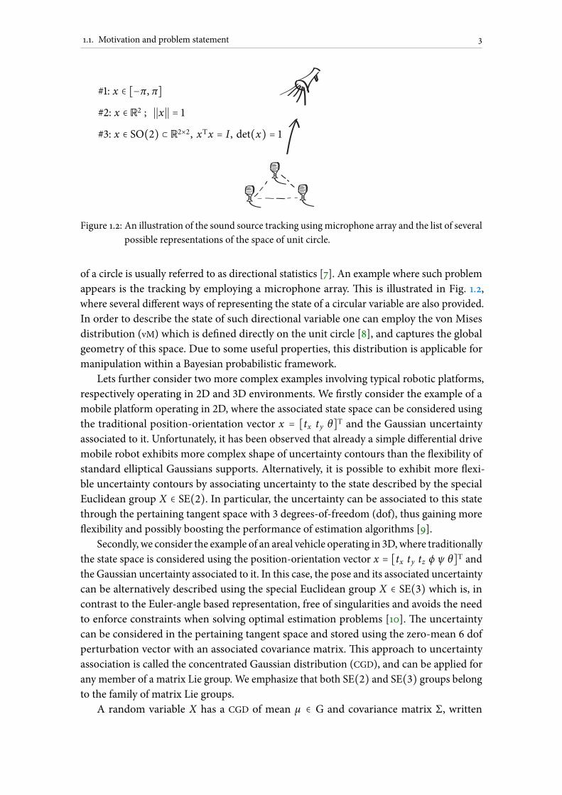
Figure 1.2: An illustration of the sound source tracking using microphone array and the list of several
possible representations of the space of unit circle.
of a circle is usually referred to as directional statistics [7]. An example where such problem
appears is the tracking by employing a microphone array.is is illustrated in Fig. 1.2,
where several dierent ways of representing the state of a circular variable are also provided.
In order to describe the state of such directional variable one can employ the von Mises
distribution (vM) which is dened directly on the unit circle [8], and captures the global
geometry of this space. Due to some useful properties, this distribution is applicable for
manipulation within a Bayesian probabilistic framework.
Lets further consider two more complex examples involving typical robotic platforms,
respectively operating in 2D and 3D environments. We rstly consider the example of a
mobile platform operating in 2D, where the associated state space can be considered using
the traditional position-orientation vector x = [tx ty θ]T and the Gaussian uncertainty
associated to it. Unfortunately, it has been observed that already a simple dierential drive
mobile robot exhibits more complex shape of uncertainty contours than the exibility of
standard elliptical Gaussians supports. Alternatively, it is possible to exhibit more exi-
ble uncertainty contours by associating uncertainty to the state described by the special
Euclidean group X ∈ SE(2). In particular, the uncertainty can be associated to this state
through the pertaining tangent space with 3 degrees-of-freedom (dof), thus gaining more
exibility and possibly boosting the performance of estimation algorithms [9].
Secondly, we consider the example of an areal vehicle operating in 3D,where traditionally
the state space is considered using the position-orientation vector x = [tx ty tz ϕ ψ θ]T and
the Gaussian uncertainty associated to it. In this case, the pose and its associated uncertainty
can be alternatively described using the special Euclidean group X ∈ SE(3) which is, in
contrast to the Euler-angle based representation, free of singularities and avoids the need
to enforce constraints when solving optimal estimation problems [10].e uncertainty
can be considered in the pertaining tangent space and stored using the zero-mean 6 dof
perturbation vector with an associated covariance matrix.is approach to uncertainty
association is called the concentrated Gaussian distribution (CGD), and can be applied for
any member of a matrix Lie group. We emphasize that both SE(2) and SE(3) groups belong
to the family of matrix Lie groups.
A random variable X has a CGD of mean µ ∈ G and covariance matrix Σ, written

4 1. introduction
X ∈SE(2)=(R t
0 1) ∣ R, t ∈ SO(2) × R2
SO(2)=R ⊂ R2×2 ∣RTR = I, det(R) = 1
X ∈SE(3)=(R t
0 1) ∣ R, t ∈ SO(3) × R3
SO(3)=R ⊂ R3×3 ∣RTR = I, det(R) = 1
Figure 1.3: Lie group representation of the state of a dierential drive mobile robot considered in 2D
(X ∈ SE(2), le, with accompanied uncertainty contours illustrated in grey for Gaussianand black for CGD) and an aerial vehicle considered in 3D (X ∈ SE(3), right).
X ∼ G (µ, Σ), if
X = µ exp∧G(ξ) and ξ ∼ N (0, Σ) (1.1)
where exp∧G performs mapping from the Euclidean space (tangent space of the Lie group
referred to as Lie algebra) to Lie group G. Other important examples of Lie groups of interest
are special orthogonal group SO(2) and SO(3), special unitary group SU(2), invertible
matrices, homographies, similarity transformations, etc [11].e two previously discussed
examples involving dierential drive mobile robot and an aerial vehicle are illustrated in
Fig. 1.3.
e vM captures the geometry of the unit circle in a global manner, but due to various
limiting factors such global approach may not be possible for an arbitrary manifold. On
the other hand, the approaches relying on CGD can at least locally account for the state
space geometry and thus boost the performance of estimation algorithms regarding both
ease and stability of implementation and the overall accuracy.is thesis questions if the
world in the surrounding of an autonomous system can be assumed to be Euclidean, and
develops approaches for dealing with eventually non-Euclidean nature of state space for
various types of objects, but also dierent measurements which arise on non-Euclidean
manifolds including microphone arrays, radar units or camera systems.
1.2 original contributions
Four original contributions of the thesis essentially revolve about probabilistic estimation
methods suitable for operating on variables arising on Lie groups rather than the Euclidean
space.e scientic contributions of this thesis resulting from the performed research are:
#1 Method for multiple moving objects tracking on the unit sphere based on the von
Mises distribution and the random nite sets.
#2 Method for moving object tracking in the space of the special Euclidean group based
on the extended Kalman lter on Lie groups.
#3 Extended information Kalman lter for state estimation on matrix Lie groups.

1.3. Outline of the thesis 5
#4 Method formultiplemoving objects tracking on LieGroups based on the concentrated
Gaussian distribution and the random nite sets.
A more detailed discussion on the scientic contributions of the thesis is given in Sec. 4.
1.3 outline of the thesis
e thesis is organized into seven chapters. Among them, two chapters particularly provide
the background material of the thesis. Aer discussing the main results of the thesis and
providing some concluding remarks, contributing publications are included in the thesis.
Hereaer, we present the outline of the thesis with a short summary of the contents.
Ch 2 is chapter presents the general mathematical background and sets up the context
of the problem of probabilistic estimation on manifolds.e introductory part of the
chapter reveals the problematic of (i) computational potential of ltering methods in
forms of Kalman and information lters, and (ii) discusses the potential of global vs.
local approaches to accounting for the non-Euclidean geometry of considered vari-
ables. Aerwards, some basic background material including the Bayesian recursion,
extended Kalman and extended information lter is provided. Finally, the basics on
global circular statistics and local approach to estimation on Lie groups is presented.
Ch 3 is chapter comprises the methods for multiple moving objects tracking, by provid-
ing an extensive overview of both traditional and widely accepted methods, as well as
recent approaches. Aerwards, it provides some underlying ideas of the probabilis-
tic hypothesis density (PHD) lter and provides an approximation of this lter for
nonlinear systems based on the Gaussian mixture and the extended Kalman lter.
Since manipulation with mixtures of distributions represents an essential task in
many multiple objects tracking applications, here we provide a brief recapitulation
of techniques for component number reduction. Finally, we describe the optimal
subpattern assignment (OSPA) metric for evaluation of the multiple objects tracking
algorithms.
Ch 4 A description of the main scientic contributions of the thesis is given here.
Ch 5 is chapter brings the conclusions of the thesis and presents some ideas for future
work from the viewpoint of open theoretical questions, application perspective and
evaluation challenges.
Ch 6 Here we include the list of publications contributing the main results of the thesis.
Ch 7 is chapter gives a statement on the author’s contribution to each of the included
publications.
Aer the seven chapters follows the list of referenced bibliography. Finally, the publications
giving the main results of the thesis which were previously published in peer-reviewed
journals or in proceedings of international scientic conferences are included.

2Probabilistic state estimation on manifolds
Probabilistic state estimation has been widely accepted approach in a variety of
engineering problems and scenarios in both traditional application domains including
tracking and surveillance, aerospace engineering, telecommunications and medicine, as
well as in some modern elds such as computer vision, speech recognition and many others.
Probabilistic approaches pay tribute to the uncertainty in perception, by relying on a key
idea of representing the uncertainty in an explicit manner using the calculus of probability
theory [1]. A long history of research in this eld experienced appearance of many dierent
estimation methods, designed for dierent use-cases depending on the (i) (non)linearity of
system model, (ii) the characteristics of underlying statistics as well as (iii) the state space
geometry of the variables of an estimation interest that are possibly non-Euclidean.
2.1 introduction
2.1.1 Probabilistic state estimation
e nature of applications of our interest cover such cases where the full or partial obser-
vations of the system occur sequentially at time instants k ∈ N, while in the meantime the
system is assumed to follow some motion model. Hence we aim to consider estimation ap-
proaches which recursively apply (i) the prediction/propagation step relying on the assumed
motion/propagation model and (ii) the correction/update step employing measurements
once they become available. In this thesis, the processes will follow either continuous or
discrete motion models, while the update will usually be given with measurements at some
discrete time instant.e background idea of the overall random variable estimation of our
interest is called Bayesian since its implementation is grounded in the Bayes theorem [12].
is enables us to build-in some (i) prior knowledge on the value of the considered random
variable, (ii) the uncertain motion model which the variable is expected to follow, and (iii)
the uncertain measurement model which the sensor is expected to follow.
⊳ kalman filtering. Probably the most important application of the Bayesian re-
cursion is the Kalman lter (KF), and majority of Bayesian approaches used nowadays
are somehow built upon the similar assumptions used in the KF’s original derivation. In
particular, the KF was presented in seminal works of Kalman [5], and Kalman and Bucy [13],
originally developed for linear systems described with Gaussian statistics and evolving on
Euclidean space. Although it was originally derived for a linear problem, the Kalman lter is
6
2.1. Introduction 7
habitually applied with impunity and considerable success to many nonlinear problems [14].
is extensions are introduced in [15] and are generally called the extended Kalman lter
(EKF). Over time, many other methods designed following the basic concepts of KF have
also appeared. Some prominent examples are iterative extended Kalman lter (IEKF) [16],
unscented Kalman lter (UKF) [17, 18, 19], cubature Kalman lter (CKF) [20, 21], quadrature
Kalman lter (QKF) [22, 23], and many others. Also, if the underlying distribution is not
Gaussian and if it is possibly multimodal then dierent approaches relying on particle
[24] and mixture lters [25, 26] need to be utilized. However, since the thesis focuses on
unimodal EKF-like approaches, we do not provide the exhaustive overview of other ltering
methods.
⊳ information filtering. From the viewpoint of processing complexity, another
important aspect of Bayesian ltering is the information lter (IF), which is the dual of the
KF. It is as well relying on the state representation by a Gaussian distribution [27] and is
the subject of the same assumptions underlying the KF. While the KF is represented by the
rst two moments, i.e., mean and covariance, the IF relies on the canonical parametrization
consisting of an information matrix and information vector [28]. As well as KF, IF operates
cyclically in two steps: the prediction and update step.e main characteristics which
make signicant dierence between the two parameterizations lie in the complexity of
the prediction and update steps.e advantage of the IF lies in the update step when the
number of measurements is larger than the size of the state space, since in this case the
update step is additive. In contrast, when the opposite applies, the prediction step is additive
and computationally less complex for the KF. Hence, what is computationally complex in one
parameterization turns out to be simple in the other (and vice-versa) [1].e most common
extension of the linear IF to non-linear systems is following similar linearization approach
as in the vein of EKF.e resulting lter is called the extended information lter (EIF) [27].
Respecting dierent applications and dierent types on non-linearity, various strategies
have been developed within the information form framework over time.is includes
sigma-point information lter [29], square-root information lter [30, 31, 32], unscented
information lter (UIF) [33], sparse extended information lter (SEIF) [34], exactly sparse
delayed-state lter (ESDSF) [35], etc.
2.1.2 Estimation on manifolds
Apart from the non-linearity of the motion and measurement models, for the overall
estimation performance it is important to account for the state space geometry and the
association of uncertainty when the underlying space is not Euclidean.is is motivated
by theoretical and implementation diculties caused by treating a constrained problem
naively with Euclidean tools. Hence recently, many works have been dedicated to associating
uncertainty to, and estimating the state of, non-Euclidean systems.
⊳ estimation of circular variables. Working with directional data, especially
under uncertainty, imposes a problem on how to represent them in a probabilistic frame-
work.is subject matter is usually referred to as directional statistics [7], since it mainly

8 2. probabilistic state estimation on manifolds
studies the observations which are unit vectors either in the plane where the sample space
will be a circle, or in the three dimensional space where the sample space will be a sphere.
e robotics community has already recognized the benets of the directional distributions
applied for modeling directional data. Although the approaches which rely on wrapped
distributions were still recently successfully used in dierent applications [36, 37], the desire
for globally capturing the entire geometry of the state space inuenced more intensive
employment of directional distributions. Some early applications of the vM distribution
dened on the unit circle [8] were presented in [38] where it was used for odometry eval-
uation in order to deal with the heading changes for topological model learning. Later,
in [39] authors proposed a solution for solving large-scale partially observable Markov
decision processes applying the same distribution. In [40, 41, 42, 43], the same distribution
was used in the context of a single speaker localization and tracking in order to model the
state and the microphone array measurements as a vMmixture and evaluated in the context
of Bayesian estimation framework.is distribution has also been successfully applied
for people trajectory shape analysis [44], radar processing [45], and a multitarget tracking
application [46].
e von Mises-Fisher distribution [47] is dened on a unit hypersphere, and hence vM
is also sometimes considered only as its special case. It was already utilized in applications
like single target tracking [48], as well as in multitarget tracking applications [49]. Another
distribution which can be considered as directional is a Bingham distribution used for de-
scribing the inference directly on the space of quaternions. It actually models variables with
180 symmetry, and was used in [50, 51, 52] and in [53] where, furthermore, a second-order
lter was derived which included also the rotational velocity.ese approaches, advocating
the unit hypersphere as the appropriate ltering space, showed better performance of the
Bingham lter and the underlying global estimation approach with respect to the EKF.
From the engineering perspective, distributions dened directly over the entire space of
interest seem to be attractive since they are able to globally capture the state space geometry,
but unfortunately their practical applicability is oen very limited. An important question
arises regarding the possibility of evaluating the pdf normalization constants in closed form.
is issue makes the Bayes prediction and correction hard to evaluate in the closed form as
well. However, the vM distribution contains some properties that could be easily exploited
within the Bayesian framework, which make it applicable for practical use. In this thesis we
analyze the directional multitarget application for 2D case, relying on the vM distribution,
which is hence more formally introduced in Sec. 2.4.1.
⊳ estimation on lie groups. Some of the most prominent examples of the non-
Euclidean geometries are the orientation and the pose of a rigid body mechanical systems.
Lie groups are natural ambient (state) spaces for description of such systems.e orientation
of a rigid body is oen described using special orthogonal groups SO(2) or SO(3) as 2– and
3–dimensional counterparts.e pose is oen represented with special Euclidean groups
SE(2) or SE(3), where again they represent 2– and 3–dimensional counterparts [54, 55].
Respecting the eld of robotics, the SE groups have been used from the very early days,
while associating the uncertainty came into focus later [56].e most oen used concept
for associating the uncertainty to Lie groups is the concept of CGD, which assumes that the
2.1. Introduction 9
eigenvalues of covariance are small, hence almost all the mass of distribution is contained
around the mean value [57, 58].
From the application perspective, an early example of error propagation on the SE(3)
group with applications to manipulator kinematics was presented in [59].erein the
authors developed a closed-form solution for the convolution of the CGDs on SE(3). In [57]
the authors proposed a solution to Bayesian fusion on Lie groups by assuming conditional
independence of observations on the group, thus setting the fusion result as a product of
CGDs, and nding the single CGD parameters which are closest to the beginning product.
One of the rst signicant works which combines both, uncertainty propagation and fusion
on the group, was presented in [10], where authors exclusively deal with the SE(3) group. A
more general approach proposed for dealing with any matrix Lie groups in the vein of the
‘classical’ EKFwas proposed in [60].erein authors derived a nonlinear continuous-discrete
extendedKalman lter on Lie groups (LG-EKF), meaning that the prediction step is presented
in the continuous domain, while the update step is discrete. In an earlier publication [61],
the authors presented a discrete version of the LG-EKF. Another approach to a nonlinear KF
on manifolds was presented in [62]. It iss designed to operate on a wider range of manifolds
than LG-EKF, and is following the ideas of the unscented transform and the UKF itself.
Some works have also addressed the uncertainty on the SE(2) group proposing new
distributions [52, 63], but these approaches still do not provide a closed-form Bayesian
recursion framework for both the prediction and update that can include non-linear models.
Additionally, in [64] authors use Gaussian process kernels for estimating the 6 dof motion
of an UAV, while in [65] authors study the appearance of multi-modal pdfs on SO and SE
groups and propose an approach relying on mixtures of projected Gaussians.
Another important group is a 3D similarity transform Sim(3) which represents an
extension of SE(3), but includes an additional parameter referred as scaling factor. Such
group may be appropriately employed in mono-vision SLAM tasks when the scale is not
known [66].e quaternions have also been previously mentioned in the context of circular
variables, and it was also noted that the Bingham distribution can globally capture the
nature of this space. However, quaternions are also members of Lie groups and can be
represented in matrix form as they are isomorphic to the special unitary group SU(2)
[11]. Alongside circular variables and Lie groups which are in the focus of the thesis, there
also exist a variety of manifolds signicant for the engineering community, and alongside
this idea several approaches for ltering on such manifolds were developed.is includes
Grassmann manifolds [67, 68], Riemannian Manifolds [69, 70], Stiefel manifolds [71], and
other specic types of manifolds [72, 73].
2.1.3 Application signicance
⊳ pose estimation. Pose and ego-motion estimation represent some of the most
prominent examples of employment of manifold approaches. In [74] authors studied the
problem of registering local relative pose estimates to produce a global consistent trajectory
of a moving robot relying on probabilistic uncertainties associated to Lie groups. Authors
in [9] specically study the uncertainty of a motion of a two-wheeled robot and discuss
the signicance of associating the uncertainty to variables on the groups, rather than the

10 2. probabilistic state estimation on manifolds
Euclidean space. In [75] authors study error growth in position estimation from noisy
relative pose measurements by carefully accounting for the geometry of the SE(2) and
SE(3) groups. In [62] authors demonstrate the lter on a synthetic dataset addressing the
problem of trajectory estimation by posing the system state to reside on the manifold
combining Euclidean space with an SO(3) group, while in the end they also demonstrate
their approach on SLAM application relying on graph optimization.
In [76] authors perform fusion of optical ow and inertial measurements for robust
egomotion estimationmodifying theUKF by following the similar approach as was proposed
by [62], and applying it for a legged robot application.e same application was developed
in [77], and the same estimation approach was used, although dierent sensor setup was
employed. Alongside the estimation algorithm, in [77] the authors proposed a careful
observability analysis by employing the concept of Lie derivatives [78]. In [79] authors use
only IMU and contact information for estimating the state of the leg of a humanoid robot
and use quaternion representation and an EKF implementation. In [60], the authors have
demonstrated the eciency of the lter on a synthetic camera pose ltering problem by
forming the system state to reside on the direct product of an SO(3) group with a Euclidean
space vector representing sequentially camera orientation, object position, angular and
radial velocities. A problem of an estimation of a complex kinematic chain has also recently
been observed, and although several Euler angles-based solutions exists [80], an approach
employing Lie groups have recently been proposed [81].
A tracking task can be seen as an extension of a pose estimation problem in terms of
sources of uncertainty of a measurements. A pioneer work on tracking on manifolds was
presented in [82] where authors perform eet tracking by modeling the target motion as
a particle describing the motion on SE(3) and employing the particle ltering approach.
Another particle ltering based approach applies a rst-order autoregressive state dynamics
and use coordinate-invariant particle lter on the SE(3) group in a single-target visual
tracking application [83].
⊳ attitude estimation. Attitude also represents an important manifold from the
estimation perspective. Although suitability of Euler angle-based representation was proven
in many practical application, the presence of singularities and non-orthogonality of compo-
nents caused these algorithms to experience dierent disadvantages. Hence, recent ltering
approaches relying on SO or quaternion-based setting managed to signicantly outper-
form the traditional Euler angle-based approaches, and have become standard in dierent
application elds. In particular, in [84] author presented real-time estimation of a rigid
body orientation from measurements of acceleration, angular velocity and magnetic eld
strength by using quaternions and is one of the rst authors who carefully treats the inherent
properties of unit quaternions. Later, in [85] authors used a similar approach to attitude
estimation by employing the same sensor setup. In [86] the authors also built upon similar
ideas, and particularly derived the so-called manifold-constrained UKF. Recently, in [87]
the authors have proposed an invariant EKF applied for attitude estimation, where they
managed to systematically exploit the invariance properties to design stochastic lters on
SO(3). Although majority of approaches rely on local techniques, some approaches have
also tempted to globally account for the geometry of SO(3) group. Hence in [88] authors
2.1. Introduction 11
have used numerical parametric uncertainty techniques, noncommutative harmonic analy-
sis, and geometric numerical integration for obtaining the global uncertainty propagation
scheme for the attitude dynamics of a rigid body. In [89] author numerically solved the
Fokker-Planck equation on the SO(3) group via noncommutative harmonic analysis to
obtain computational tools to propagate a pdf over the attitude kinematics, and nally uses
it for attitude motion planning and estimation.e more in-depth survey of nonlinear
attitude estimation approaches is available in [90].
⊳ manipulator kinematics and control. An early application of associating
the uncertainty to SE(3) group was presented in [91], and later in [56].erein, the constant
position motion model was assumed, and the uncertainty is assumed to be small.is
pioneering systematic methodology of propagating and fusing spatial uncertainties was
applied for actions in an assembly task. A more careful treatment of error propagation was
later presented in [59] where more general propagation model was used. While in [59] a
rst-order error propagation on the SE(3) group was presented, the same authors have later
extended the approach to second-order error propagation [92].
ere has also been several control applications where a manifold geometry was ex-
ploited. In [93, 94] authors used the SE(3) group representation for describing the state of
steerable needle which is in the focus of their control application.ey particularly derived
the equations for parametrically propagating the uncertainty accounting for the geometry
of the SE(3) state space. Another approach relying on Lie group representation of highly
articulated robot and applied in invasive surgery was presented in [95].e position and
orientation of every robot link evolves in SE(3), while authors used the EKF implementation
such that the state vector is dened using elements of Lie algebra representation.
⊳ calibration. A popularity of quaternion based approaches has risen via time, and
many authors have tried to exploit the geometry of a quaternion state space by employing
the nonlinear propagation functions. However, in the update stepmajority of the approaches
relied on the post-normalization, and hence forced the mean to preserve the unit constraint.
Calibration is a ‘classic’ application of such quaternion based EKF or UKF approaches. In [96,
97] authors used a quaternion based EKF formulation which fuses dierent measurements
with inertial sensors and does not only estimate pose and velocity of an UAV, but also
estimates sensor biases, scale of the positionmeasurement and self (inter-sensor) calibration.
Similarly, in [98] authors combined visual and inertial sensing for navigation, with an
emphasis on the ability to self-calibrate the camera–IMU transformation, but use UKF
ltering approach. In [99] authors developed a framework for fusion of dierent sensors
allowing for their self-calibration by relying on an IEKF implementation. Alterntively to
quaternion approaches, in [100] authors performed an extrinsic calibration between two
sensors mounted rigidly on a moving body by describing the 6 dof state using SE(3) group.
A more general approach to calibration in terms of state space geometry was proposed
in [101].erein authors use non-linear optimization on constraint graphs and combine
it with a principled way of handling non-Euclidean spaces (class of box-plus spaces as in
the vein of [62]) making it particularly easy to solve non-trivial multi-sensor calibration
problems.eir developed Matlab framework is available as open source toolkit.

12 2. probabilistic state estimation on manifolds
⊳ slam. An early SLAM application accounting for the state space geometry was presented
in [102], where the state is given as a group element, while the estimation error is represented
locally by a dierential location vector.e authors refer to this concept as the symmetries
and perturbations map (SPmap), while they use the EKF implementation. Another EKF-based
SLAM using the quaternion-based approach and accounting for the state space geometry
was presented in [103], and relies on the quaternion normalization in the update step. A
direct approach to visual EKF-based SLAM which uses the SE(3) representation is presented
in [104]. In [105] the authors preintegrated a large number of inertial measurement unit
measurements for visual-inertial navigation into a single relative motion constraint by
respecting the structure of the SO(3) group and dening the uncertainty thereof in the
pertaining tangent space.
A quite prominent example of an application where the need arises for computational
benets of the IF and the geometric accuracy of Lie groups is SLAM. SLAM is of great practical
importance in many robotic and autonomous system applications since it represents a
problem of acquiring a map of an unknown environment, and simultaneously localizing
itself within the map.e earliest SLAM solutions were based on an EKF implementation
and in practice they could handle maps that contain a few hundred features, while in
many applications maps are orders of magnitude larger [34].erefore, the EIF is oen
employed and widely accepted for SLAM [106].e EIF based approaches reached its
zenith with sparsication techniques resulting withSEIF [34] and ESDSF [35]. However, the
localization component of SLAM conforms the pose estimation problem as arising on Lie
groups. Furthermore, the mapping part of SLAM consists of landmarks whose position, as
well, arises on SE(3).erefore, some recent SLAM solutions approached the problem by
respecting the geometry of the state space [107, 108, 109], since signicant cause of error in
such application was determined to stem from the state space geometry approximations.
However, these SLAM solutions, although able to account for the geometry of the state space,
exclusively rely on graph optimization [66, 110, 111], but still not on ltering approaches
(although ltering approaches have still recently been successfully used for plain odometry
applications [112, 113]).
2.1.4 Organization of the chapter
e rest of the chapter is organized as follows.e underlying background estimation
theory in the form of a Bayesian ltering is presented in Sec. 2.2.e traditional solution
to the Bayes ltering problem in the form of an extended Kalman lter and an extended
information lter, suitable for operation with Euclidean variables is given in Sec. 2.3. A basic
overview of the vM distribution is given in Sec. 2.4.e last section of this chapter provides
directions for evaluation of the LG-EKF including (i) mathematical preliminaries useful for
understanding the necessary mappings between the triplet including Lie group, Lie algebra
and Euclidean space, (ii) basics on the concept of CGD, and (iii) equations for the LG-EKF
Sec. 2.5.

2.2. Bayesian ltering 13
2.2 bayesian filtering
e Bayesian lter has a recursive form and operates in two steps. Firstly, based on the
prior knowledge and motion model, the prediction can be performed. Secondly, once the
measurement becomes available, the update step is executed.
2.2.1 Model of the system
To dene the ltering problem, we consider the evolution of the discrete system from time
instant k − 1 to k following the motion model given as
xk = f (xk−1, uk−1) +wk−1 , k ∈ N , (2.1)
where f is a nonlinear function of the system state x and control actions u at time step
k − 1, while w is process noise.e objective of estimation is to recursively estimate xk from
measurements given via another non-linear function
zk = h(xk) + vk , k ∈ N , (2.2)
where h is possibly a nonlinear function in the system state and v is a measurement noise.
2.2.2 Statistical inference
From a Bayesian perspective, the estimation problem is to recursively calculate some degree
of belief in the state x at time instant k, i.e., xk, given the measurement data zk [24].
From the perspective of the pdf, we are striving to estimate the density p(xk ∣ z1∶k), i.e.,
the pdf of the state xk given the history of all measurements z1∶k , oen referred as posterior
at time instant k.is may be obtained recursively applying the prediction and update
steps. Assuming that the posterior p(xk−1 ∣ z1∶k−1) is available, the prediction step particularly
involves calculating the prior pdf via the Chapman–Kolmogorov equation [24]
p(xk ∣ z1∶k−1) = ∫ p(xk ∣ xk−1)p(xk−1 ∣ z1∶k−1)dxk−1 , (2.3)
where p(xk ∣ xk−1) is the probabilistic model of the state evolution.
In the update step, once the measurement zk becomes available, it can be used to update
the prior via the Bayes rule
p(xk ∣ z1∶k) =p(zk ∣ xk)p(xk ∣ z1∶k−1)
p(zk ∣ z1∶k−1), (2.4)
where the pdf p(zk ∣ xk) represents our likelihood function dened by the sensor model
(2.2) and p(zk ∣ z1∶k−1) represents a normalization constant. For implementation purposes,
the three probability distributions are required; (i) the initial belief p(x0), (ii) the mea-
surement probability p(zk ∣ xk), (iii) state transition probability p(xk ∣ xk−1).is recursive
propagation of the posterior density is only a conceptual solution, while in general it cannot
be determined analytically. However, solutions do exist in a restrictive set of cases which
will be briey introduced in the thesis [24]. Furthermore, one should note that there is
nothing intrinsic in the Bayesian lter propagation and update steps that would limit this
concept to operating on Euclidean spaces only.is thesis shows several applications of
this concept in various non-Euclidean problems.
14 2. probabilistic state estimation on manifolds
2.2.3 Validation gate
e normalization constant p(zk ∣ z1∶k−1) results from applying the marginalization of the
state xk from the nominator of (2.4) as
p(zk ∣ z1∶k−1) = ∫ p(zk ∣ xk)p(xk ∣ z1∶k−1)dxk . (2.5)
is probability can further be used for validation gate purposes, so as to reject highly
unlikely measurements/outliers. In particular, the validity of a measurement zk is directly
evaluated through (2.5) [114].
2.3 traditional probabilistic state estimation
Since the concept of Kalman ltering represents an important aspect of this thesis, the EKF
is briey presented in the sequel.
2.3.1 Extended Kalman lter
Let us assume that the system is given with motion (2.1) andmeasurement models (2.2), and
process and measurement noises are Gaussian given as wk ∼ N (0,Qk), vk ∼ N (0, Rk). We
also assume the system state and measurement spaces are Euclidean, i.e., xk ∈ Rn, zk ∈ Rm,
∀k ∈ N . If the posterior at time instance k−1 is a Gaussian distribution xk−1 ∼ N (µk−1, Σk−1),
the predicted state xk∣k−1 is given with parameters
µk∣k−1 = f (µk−1, uk−1) (2.6)
Σk∣k−1 = Fk−1Σk−1FTk−1 + Qk−1 ,
where F is state transition matrix dened to be the Jacobian
Fk−1 =∂ f
∂x∣x=µk−1
. (2.7)
Having the estimated prior xk∣k−1 ∼ N (µk∣k−1, Σk∣k−1), once having the measurement zk
available, the updated state of the system is evaluated as
Kk = Σk∣k−1HTk (HkΣk∣k−1H
Tk + Rk)
−1 (2.8)
µk = µk∣k−1 + Kk(zk −Hkµk∣k−1)
Σk = (I − KkHk)Σk∣k−1 ,
where H is measurement matrix dened to be the Jacobian
Hk =∂h
∂x∣x=µk∣k−1
. (2.9)
A complete and intuitive derivation of KF is available in [1].
When considering the validation gating, the validity of a measurement is determined
from its residual (or innovation) with the predicted observation, which results from (2.5)
producing a Gaussian distribution of the innovation as [106]
N (zk −Hkµk∣k−1,HkΣk∣k−1HTk + Rk) . (2.10)

2.3. Traditional probabilistic state estimation 15
Validation is computed by gating the normalized innovation squared (NIS; also commonly
known as the Mahalanobis distance) as
(zk −Hkµk∣k−1)T(HkΣk∣k−1H
Tk + Rk)
−1(zk −Hkµk∣k−1) ≤ χ2d , (2.11)
where χ2 is a chi-square pdf, and d is innovation dimension.
e above recursion results from the rst-order Taylor series expansion of nonlinear
motion and measurement models, and although higher-order EKF [115] exist, its practical
usage is not nearly as oen as rst-order based approximation [27].
2.3.2 Extended Information lter
While KF relies on moment representation of Gaussian distributions using mean µ and
covariance Σ parameters, the IF replaces themwith canonical parameters called information
vector y and information matrix Y .e relation between the two set of parameters are
given as
Nc(y,Y) = Nc(Σ−1µ, Σ−1) , Nm(µ, Σ) = Nm(Y
−1y,Y−1) , (2.12)
where index m denotes the moment representation, while c represents the canonical repre-
sentation. Since moment representation is considered ‘classical’, in the rest of the thesis we
omit specically using index m when referring to it.
Given the same assumptions as in the EKF case about motion and measurement models,
and if the posterior at time instance k − 1 is a Gaussian distribution given with canonical
parameters xk−1 ∼ Nc(yk−1,Yk−1), the predicted state xk∣k−1 is calculated as
µk∣k−1 = f (Y−1k−1y, uk−1) (2.13)
Yk∣k−1 = (Fk−1Y−1k−1F
Tk−1 + Qk−1)
−1
yk∣k−1 = Yk∣k−1µk∣k−1 ,
where F is state transition matrix dened as in the EKF case. Having the estimated prior
xk∣k−1 ∼ Nc(yk∣k−1,Yk∣k−1), once having the measurement zk available, the updated state of
the system is calculated as
yk = yk∣k−1 +HTkR−1k (zk − h(µk∣k−1) +Hkµk∣k−1) (2.14)
Yk = Yk∣k−1 +HTkR−1k Hk ,
whereH is measurementmatrix dened as in the EKF case. Furthermore, ifN measurements
are available at time step k through dierent measurement models hi and measurement
noise r ik∼ N (0, Ri ,k), the updated information vector and matrix become
yk = yk∣k−1 +N
∑i=1
HTi ,kR−1i ,k(zi ,k − hi(µk∣k−1) +Hi ,kµk∣k−1) ,
Yk = Yk∣k−1 +N
∑i=1
HTi ,kR−1i ,kHi ,k .
(2.15)
16 2. probabilistic state estimation on manifolds
2.4 directional estimation
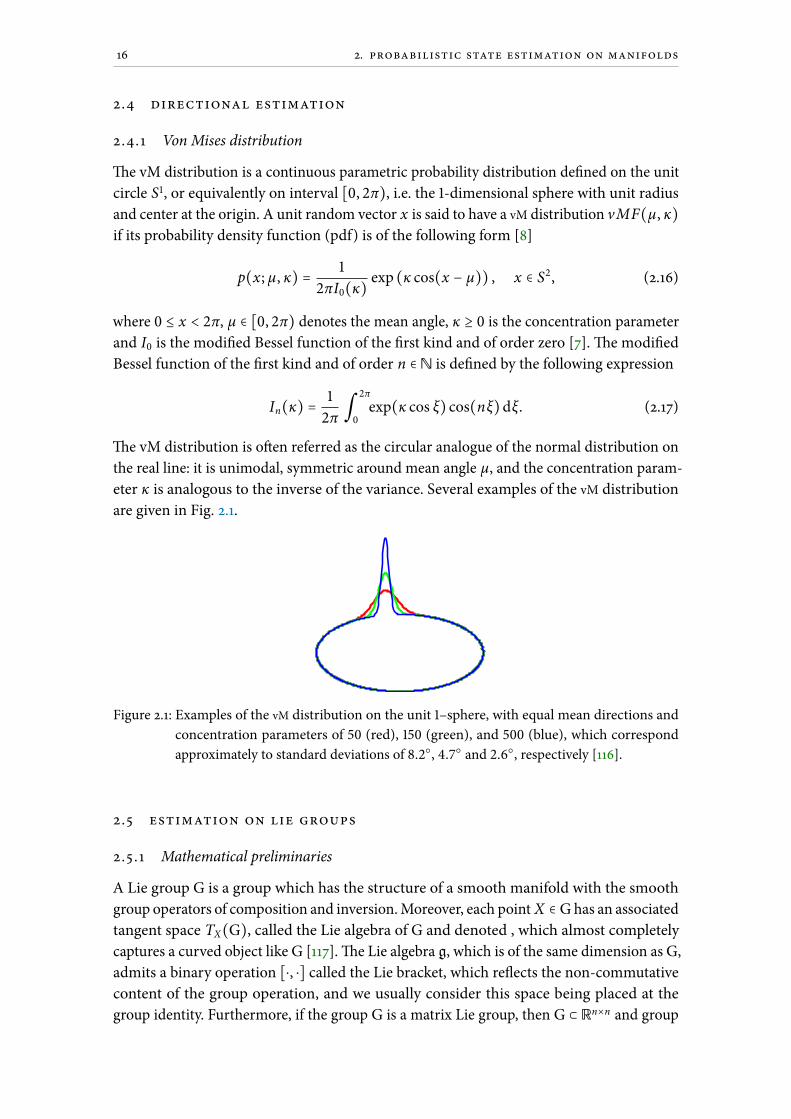
2.4.1 Von Mises distribution
e vM distribution is a continuous parametric probability distribution dened on the unit
circle S1, or equivalently on interval [0, 2π), i.e. the 1-dimensional sphere with unit radius
and center at the origin. A unit random vector x is said to have a vM distribution vMF(µ, κ)
if its probability density function (pdf) is of the following form [8]
p(x; µ, κ) =1
2πI0(κ)exp (κ cos(x − µ)) , x ∈ S2, (2.16)
where 0 ≤ x < 2π, µ ∈ [0, 2π) denotes the mean angle, κ ≥ 0 is the concentration parameter
and I0 is the modied Bessel function of the rst kind and of order zero [7].e modied
Bessel function of the rst kind and of order n ∈ N is dened by the following expression
In(κ) =1
2π ∫ 2π0
exp(κ cos ξ) cos(nξ)dξ. (2.17)
e vM distribution is oen referred as the circular analogue of the normal distribution on
the real line: it is unimodal, symmetric around mean angle µ, and the concentration param-
eter κ is analogous to the inverse of the variance. Several examples of the vM distribution
are given in Fig. 2.1.
Figure 2.1: Examples of the vM distribution on the unit 1–sphere, with equal mean directions and
concentration parameters of 50 (red), 150 (green), and 500 (blue), which correspond
approximately to standard deviations of 8.2, 4.7 and 2.6, respectively [116].
2.5 estimation on lie groups
2.5.1 Mathematical preliminaries
A Lie group G is a group which has the structure of a smooth manifold with the smooth
group operators of composition and inversion.Moreover, each point X ∈ Ghas an associated
tangent space TX(G), called the Lie algebra of G and denoted , which almost completely
captures a curved object like G [117].e Lie algebra g, which is of the same dimension as G,
admits a binary operation [⋅, ⋅] called the Lie bracket, which reects the non-commutative
content of the group operation, and we usually consider this space being placed at the
group identity. Furthermore, if the group G is a matrix Lie group, then G ⊂ Rn×n and group

2.5. Estimation on Lie groups 17
Figure 2.2: An illustration of mappings within the triplet of Lie group G – Lie algebra g – Euclidean
space Rp [121].
operations are simply matrix multiplication and inversion. Although not all Lie groups are
matrix groups, the majority of them has an equivalent matrix representation—especially
the ones considered in physical sciences [60]. Moreover, the theorem [118] says that every
Lie algebra is isomorphic to a matrix Lie algebra, thus we will simply say ‘Lie algebra’ rather
than ‘matrix Lie algebra’.
e Lie algebra g ⊂ Rn×n associated to a p-dimensional matrix Lie group G ⊂ Rn×n is a
p-dimensional vector space dened by a basis consisting of p real matrices Er, r = 1, . . . , p,
oen referred to as generators [119]. In particular, a Lie algebra is an open neighbourhood
around 0p in the tangent space of G at the identity In.e matrix exponential expGand
matrix logarithm logGestablish a local dieomorphism between G and g as
expG∶ g→ G and log
G∶ G→ g. (2.18)
Furthermore, a natural relation exists between the p-dimensional Lie algebra g and the
Euclidean space Rp, and is given through a linear isomorphism
[⋅]∨G ∶ g→ Rp and [⋅]∧G ∶ R
p → g. (2.19)
For brevity, we will use the notation in the vein of [120]
exp∧G(x) = exp
G([x]∧G) and log
∨G(X) = [log
G(X)]∨G, (2.20)
where x ∈ Rp and X ∈ G. An illustration of these concepts is given in Fig. 2.2.
Lie groups are generally non-commutative, i.e., XY ≠ YX. However, the non-commutativity
can be captured by the so-called adjoint representation of G on g [58]
X exp∧G(y) = exp∧
G(AdG(X)y)X , (2.21)
which can be seen as a way of representing the elements of the group as a linear transforma-
tion of the group’s algebra.e adjoint representation of g, adG, is in fact the dierential
of AdG at the identity. Another important result for working with Lie group elements is
the Baker-Campbell-Hausdor (BCH) formula, which enables representing the product of
Lie group members as a sum in the Lie algebra. We will use the following BCH formulae
[122, 58]
log∨G(exp∧
G(x) exp∧
G(y)) = y + φG(y)x + O(∣∣y∣∣2), (2.22)
log∨G(exp∧
G(x + y) exp∧
G(−x)) = ΦG(x)y + O(∣∣y∣∣2), (2.23)
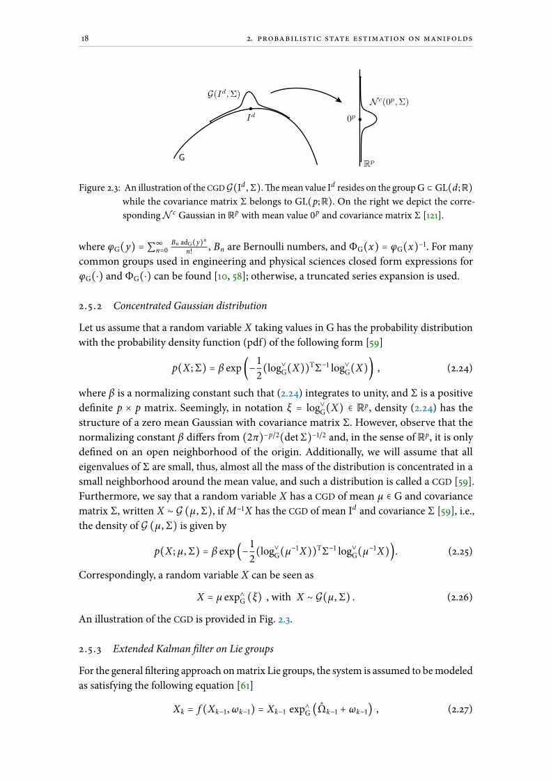
18 2. probabilistic state estimation on manifolds
Figure 2.3: An illustration of theCGDG(Id , Σ).emean value Id resides on the groupG ⊂ GL(d;R)while the covariance matrix Σ belongs to GL(p;R). On the right we depict the corre-spondingN c Gaussian in Rp with mean value 0p and covariance matrix Σ [121].
where φG(y) = ∑∞n=0
Bn adG(y)nn!
, Bn are Bernoulli numbers, and ΦG(x) = φG(x)−1. For many
common groups used in engineering and physical sciences closed form expressions for
φG(⋅) and ΦG(⋅) can be found [10, 58]; otherwise, a truncated series expansion is used.
2.5.2 Concentrated Gaussian distribution
Let us assume that a random variable X taking values in G has the probability distribution
with the probability density function (pdf) of the following form [59]
p(X; Σ) = β exp(−1
2(log
∨G(X))TΣ−1 log∨
G(X)) , (2.24)
where β is a normalizing constant such that (2.24) integrates to unity, and Σ is a positive
denite p × p matrix. Seemingly, in notation ξ = log∨G(X) ∈ Rp, density (2.24) has the
structure of a zero mean Gaussian with covariance matrix Σ. However, observe that the
normalizing constant β diers from (2π)−p/2(det Σ)−1/2 and, in the sense of Rp, it is only
dened on an open neighborhood of the origin. Additionally, we will assume that all
eigenvalues of Σ are small, thus, almost all the mass of the distribution is concentrated in a
small neighborhood around the mean value, and such a distribution is called a CGD [59].
Furthermore, we say that a random variable X has a CGD of mean µ ∈ G and covariance
matrix Σ, written X ∼ G (µ, Σ), ifM−1X has the CGD of mean Id and covariance Σ [59], i.e.,
the density of G (µ, Σ) is given by
p(X; µ, Σ) = β exp (−1
2(log
∨G(µ−1X))TΣ−1 log∨
G(µ−1X)). (2.25)
Correspondingly, a random variable X can be seen as
X = µ exp∧G(ξ) , with X ∼ G(µ, Σ) . (2.26)
An illustration of the CGD is provided in Fig. 2.3.
2.5.3 Extended Kalman lter on Lie groups
For the general ltering approach onmatrix Lie groups, the system is assumed to bemodeled
as satisfying the following equation [61]
Xk = f (Xk−1,ωk−1) = Xk−1 exp∧G(Ωk−1 + ωk−1) , (2.27)
2.5. Estimation on Lie groups 19
where Xk ∈ G is the state of the system at time k, G is a p-dimensional Lie group, ω ∼
NRp(0p×1,Q) is white Gaussian noise and Ω = Ω(X) ∶ G→ Rp is a non-linear C2 function.
e prediction step of the LG-EKF, based on the motion model (2.27), is governed by
the following formulae
µk∣k−1 = µk−1 exp∧G(Ωk−1) (2.28)
Σk∣k−1 = Fk−1Σk−1FTk−1 +ΦG(Ωk−1)Qk−1ΦG(Ωk−1)
T , (2.29)
where µ ∈ G and Σ ∈ Rp×p are predicted mean value and the covariance matrix, respectively,
hence the state remains G–distributed Xk∣k−1 ∼ G(µk∣k−1, Σk∣k−1).e operator F , a matrix
Lie group equivalent to the Jacobian of f (X , n), and ΦG are given as follows
Fk−1 = AdG (exp∧G(−Ωk−1)) +ΦG(Ωk−1)Ck−1 (2.30)
ΦG(a) =∞∑m=0
(−1)m
(m + 1)!adG(v)m , a ∈ Rp (2.31)
Ck−1 =∂
∂ξΩ (µk−1 exp
∧G(ξ))∣ξ=0 . (2.32)
e discrete measurement model on the matrix Lie group is modelled as
Zk = h(Xk) exp∧G′ (mk) , (2.33)
where Zk ∈ G′, h ∶ G→ G′ is a C1 function and mk ∼ NRq(0q×1, Rk) is white Gaussian noise.
e update step of the lter, based on the measurement model (2.33), strongly resembles
the standard EKF update procedure, relying on the Kalman gain Kk and innovation vector
νk calculated as follows
Kk = Σk∣k−1HTk (HkΣk∣k−1H
Tk + Rk)
−1
νk = Kk (log∨G′ (h(µk∣k−1)
−1Zk)) . (2.34)
e matrixHk can be seen as the measurement matrix of the system, i.e., a matrix Lie group
equivalent to the Jacobian of h(Xk), and is given as
Hk =∂
∂ξ[log
∨G′ (h(µk∣k−1)
−1h (µk∣k−1 exp∧G(ξ)))]∣ξ=0 . (2.35)
Finally, having dened all the constituent elements, the update step is calculated via
µk = µk∣k−1 exp∧G(νk) (2.36)
Σk = ΦG(νk) (Ip×p − KkHk)Σk∣k−1ΦG(νk)
T . (2.37)
As in the case of the prediction step, the state Xk+1 ∼ G(µk , Σk) remains G–distributed aer
the correction as well. For a more formal derivation of the LG-EKF, the interested reader is
referred to [61] and [121].

3Moving objects tracking based on random nite
sets
Multiple objects tracking has a long history spanning over 50 years referring to
the problem of jointly estimating the trajectories, e.g., position and orientation as
well as their respective velocities and accelerations, and the number of objects in the space,
relying on the observations from sensor data. Driven by aerospace applications in the 1960’s,
it nds its application in diverse traditional engineering disciplines such as intelligence,
surveillance and reconnaissance, radar/sonar applications, air trac control, etc. During the
last decade, advances in MOT techniques along with sensing and computing technologies,
have opened up numerous research venues such as robotics and autonomous systems,
computer vision, biomedical research, agriculture and forestry, epidemiology and public
health, communications networks, oceanography, remote sensing, etc [123].
3.1 introduction
From the viewpoint of the several sources of uncertainty appearances (described in Ch.1)
among whom each appears challenging itself, data association attracted probably the most
signicant attention of the overall research community.e reasoning might lie in the fact
that all other sources of uncertainty can be considered as special cases of the data association
task. For example, one can contend with the recognition of births and deaths only once the
data association task gures out that the existing list of recognized objects does not match
the evolving observations well. Furthermore, false positive and false negative observations,
i.e., false alarms andmissed detections, can also be considered only aer the data association
task gures out that the list of existing objects does not overlap with the observations well.
Given the previous discussion, the MOT application can be considered as a task which
aims at tracking a random number of objects receiving a random number of measurements.
Among all the existingMOT approaches, the most popular are naive global nearest neighbor
approaches (GNN) [124], the joint probabilistic data association (JPDA) [125, 126], themultiple
hypothesis tracking (MHT) [127, 128], and commonly referred to as RFS based multi-object
lters [129, 130]. Although recent developments in RFS have yielded a variety of tracking
methods that claim to avoid data association (oen referred to as data association-free
approaches), it was proven that bothMHT and JPDA can be derived within the RFS framework
[131], thus representing only special cases of RFS approaches.e research community oen
intentionally follows the terminology which inherently abuses the true relation between data
20
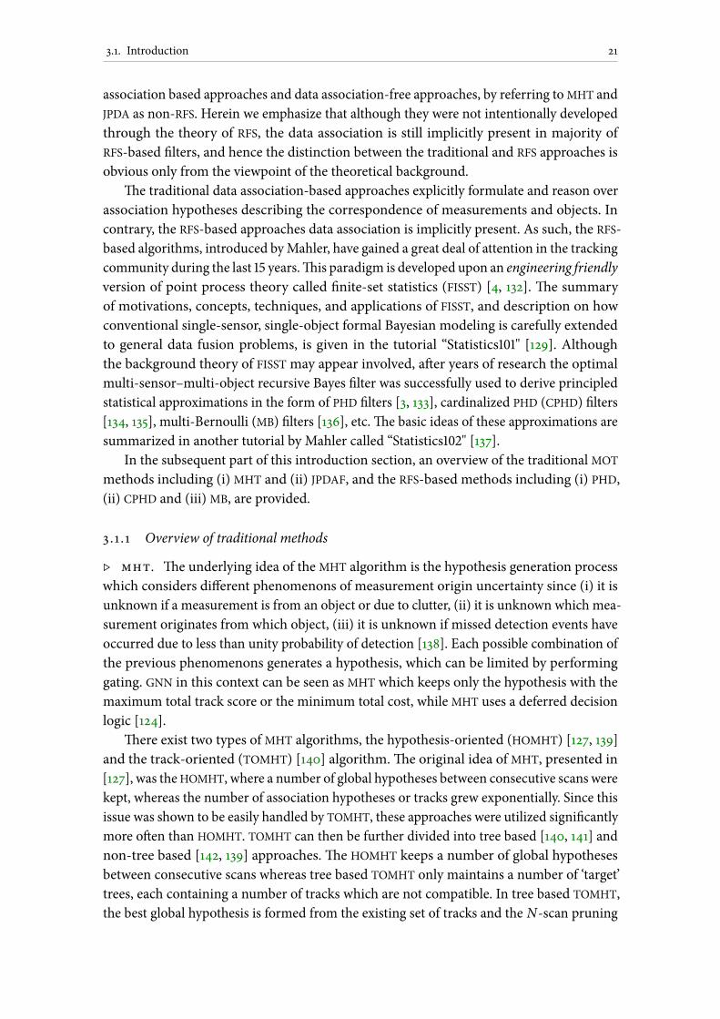
3.1. Introduction 21
association based approaches and data association-free approaches, by referring toMHT and
JPDA as non-RFS. Herein we emphasize that although they were not intentionally developed
through the theory of RFS, the data association is still implicitly present in majority of
RFS-based lters, and hence the distinction between the traditional and RFS approaches is
obvious only from the viewpoint of the theoretical background.
e traditional data association-based approaches explicitly formulate and reason over
association hypotheses describing the correspondence of measurements and objects. In
contrary, the RFS-based approaches data association is implicitly present. As such, the RFS-
based algorithms, introduced byMahler, have gained a great deal of attention in the tracking
community during the last 15 years.is paradigm is developed upon an engineering friendly
version of point process theory called nite-set statistics (FISST) [4, 132].e summary
of motivations, concepts, techniques, and applications of FISST, and description on how
conventional single-sensor, single-object formal Bayesian modeling is carefully extended
to general data fusion problems, is given in the tutorial “Statistics101" [129]. Although
the background theory of FISSTmay appear involved, aer years of research the optimal
multi-sensor–multi-object recursive Bayes lter was successfully used to derive principled
statistical approximations in the form of PHD lters [3, 133], cardinalized PHD (CPHD) lters
[134, 135], multi-Bernoulli (MB) lters [136], etc.e basic ideas of these approximations are
summarized in another tutorial by Mahler called “Statistics102" [137].
In the subsequent part of this introduction section, an overview of the traditional MOT
methods including (i) MHT and (ii) JPDAF, and the RFS-based methods including (i) PHD,
(ii) CPHD and (iii) MB, are provided.
3.1.1 Overview of traditional methods
⊳ mht. e underlying idea of the MHT algorithm is the hypothesis generation process
which considers dierent phenomenons of measurement origin uncertainty since (i) it is
unknown if a measurement is from an object or due to clutter, (ii) it is unknown which mea-
surement originates from which object, (iii) it is unknown if missed detection events have
occurred due to less than unity probability of detection [138]. Each possible combination of
the previous phenomenons generates a hypothesis, which can be limited by performing
gating. GNN in this context can be seen as MHT which keeps only the hypothesis with the
maximum total track score or the minimum total cost, while MHT uses a deferred decision
logic [124].
ere exist two types of MHT algorithms, the hypothesis-oriented (HOMHT) [127, 139]
and the track-oriented (TOMHT) [140] algorithm.e original idea of MHT, presented in
[127], was theHOMHT, where a number of global hypotheses between consecutive scans were
kept, whereas the number of association hypotheses or tracks grew exponentially. Since this
issue was shown to be easily handled by TOMHT, these approaches were utilized signicantly
more oen than HOMHT. TOMHT can then be further divided into tree based [140, 141] and
non-tree based [142, 139] approaches.e HOMHT keeps a number of global hypotheses
between consecutive scans whereas tree based TOMHT only maintains a number of ‘target’
trees, each containing a number of tracks which are not compatible. In tree based TOMHT,
the best global hypothesis is formed from the existing set of tracks and the N-scan pruning

22 3. moving objects tracking based on random finite sets
[124] and track-score based pruning are used to limit the number of tracks from growing
exponentially [138]. An early ecient implementation of the tree based TOMHT algorithm
in which the N-best hypotheses are determined in polynomial time is presented in [143].
On the other hand, a number of dierent non-tree TOMHT variants were proposed [123],
but due to the intuitive interpretation and the clarity of the tree based TOMHT, the non-tree
methods never attracted such signicant attention as tree based methods. Several dierent
varieties of the probabilisticMHT (PMHT), relying on so a posteriori probability associations
were also developed, but they never attracted signicant attention [144, 145, 146, 147]. and
since this is not in the focus of the thesis we do not consider them any further. A general
motivation for MHT, its basic principles and the alternative implementations in common
use are summarized in [128].
⊳ jpdaf. e early research on probabilistic data association approaches was exclusively
focused on single object tracking applications, accounting for some basic phenomenons
related to themeasurement origin uncertainty.e seminal paper byYaakov Bar-Shalom and
Edison Tse [125] proposed the probabilistic data association PDA approach which grounded
the basis for the entire research on probabilisticMOT research.e PDA algorithm calculates
the association probabilities to the object being tracked for each validated measurement at
the current time.e joint probabilistic data association JPDA approach is a multi-object
extension of the PDA [126], relying on the assumption that the number of tracked objects is
known.e key feature of the JPDA is that it evaluates the conditional probabilities of the joint
association events, where each event represents one combination ofmeasurements-to-object
associations. Typically the state estimation algorithm, which is carried out upon events
evaluation is calculation of marginal association probabilities.ese marginal probabilities
are obtained from the joint probabilities by summing over all joint association events in
which the marginal event of interest (respecting each object separately) occurs [148].e
state estimation equations are then decoupled among the objects and exactly the same as in
PDA. For this purpose, JPDA shows tendency that tracks of closely spaced objects become
overlapped due to the shared measurements across tracks, when this sharing lasts for
many frames or scans [148]. Alternatively, more realistic assumption accounts for possible
correlations between states of two objects aer sharing some measurements, yielding a
covariance matrix with o-diagonal blocks which reect the correlation between the state
estimation errors of the objects.is approach is called JPDA coupled lter (JPDAC).is
problem is well-known as a problem of track coalescence, and some improvements on
this topic are available in [149]. Over time, some approximations of JPDA designed for
circumventing the combinatorial complexity for large number of objects have also been
developed [150]. A tutorial on PDA and JPDA techniques is available in [148].
Mušicki et al. managed to rederive PDA without an initial assumption of track exis-
tence which was an important relaxation of the original PDA assumptions, and called the
algorithm integrated probabilistic data association IPDA [151]. As such, this algorithm simul-
taneously provides expressions for both probability of track existence and data association.
Later, Mušicki and Evans managed to extend the JPDA with the concept of object existence
probability for individual track [152] and called the algorithm joint integrated PDA (JIPDA).
is concept easily allows for track management in terms of false track discrimination or
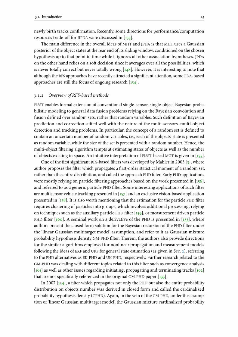
3.1. Introduction 23
newly birth tracks conrmation. Recently, some directions for performance/computation
resources trade-o for JIPDA were discussed in [153].
e main dierence in the overall ideas of MHT and JPDA is that MHT uses a Gaussian
posterior of the object states at the rear end of its sliding window, conditioned on the chosen
hypothesis up to that point in time while it ignores all other association hypotheses. JPDA
on the other hand relies on a so decision since it averages over all the possibilities, which
is never totally correct but never totally wrong [148]. However, it is interesting to note that
although the RFS approaches have recently attracted a signicant attention, some PDA-based
approaches are still the focus of ongoing research [154].
3.1.2 Overview of RFS-based methods
FISST enables formal extension of conventional single-sensor, single-object Bayesian proba-
bilistic modeling to general data fusion problems relying on the Bayesian convolution and
fusion dened over random sets, rather that random variables. Such denition of Bayesian
prediction and correction suited well with the nature of the multi-sensors–multi-object
detection and tracking problems. In particular, the concept of a random set is dened to
contain an uncertain number of random variables, i.e., each of the objects’ state is presented
as random variable, while the size of the set is presented with a random number. Hence, the
multi-object ltering algorithm tempts at estimating states of objects as well as the number
of objects existing in space. An intuitive interpretation of FISST-based MOT is given in [155].
One of the rst signicant RFS-based lters was developed by Mahler in 2003 [3], where
author proposes the lter which propagates a rst-order statistical moment of a random set,
rather than the entire distribution, and called the approach PHD lter. Early PHD applications
were mostly relying on particle ltering approaches based on the work presented in [156],
and referred to as a generic particle PHD lter. Some interesting applications of such lter
are multisensor vehicle tracking presented in [157] and an exclusive vision-based application
presented in [158]. It is also worth mentioning that the estimation for the particle PHD lter
requires clustering of particles into groups, which involves additional processing, relying
on techniques such as the auxiliary particle PHD lter [159], or measurement driven particle
PHD lter [160]. A seminal work on a derivative of the PHD is presented in [133], where
authors present the closed form solution for the Bayesian recursion of the PHD lter under
the ‘linear Gaussian multitarget model’ assumption, and refer to it as Gaussian mixture
probability hypothesis density GM-PHD lter.erein, the authors also provide directions
for the similar algorithms employed for nonlinear propagation and measurement models
following the ideas of EKF and UKF for general state estimation (as given in Sec. 2), referring
to the PHD alternatives as EK-PHD and UK-PHD, respectively. Further research related to the
GM-PHD was dealing with dierent topics related to this lter such as convergence analysis
[161] as well as other issues regarding initiating, propagating and terminating tracks [162]
that are not specically referenced in the original GM-PHD paper [133].
In 2007 [134], a lter which propagates not only the PHD but also the entire probability
distribution on objects number was derived in closed form and called the cardinalized
probability hypothesis density (CPHD). Again, In the vein of the GM-PHD, under the assump-
tion of ‘linear Gaussian multitarget model’, the Gaussian mixture cardinalized probability

24 3. moving objects tracking based on random finite sets
hypothesis density GM-CPHD lter was derived [163, 135], while it was rst applied for a
ground moving object tracking application with jointly employing digital road maps for
road constraint [164].
At this time, large part of the research community have also dealt with the problems
of estimating or learning the parameters typical for MOT applications and usually used in
both traditional and RFSs approaches, such as unknown clutter intensity [165, 166, 167, 168],
object birth intensity [160], and detection prole [167]. Also, since both PHD and CPHD
have been originally developed such that the newly birth components were induced via
a mixture of components, it was signicant to provide a relaxation of this assumption
supporting the uniform object birth model over the entire space of interest [169].ey have
also been extended to multiple models [170], extended objects [171, 172], multiple sensors,
superpositional measurements, distributed multi-object ltering, etc. [138].
Already at this early theoretical stages of development of RFS approaches, they have
attracted a signicant attention in practical applications, such as information fusion in
automotive engineering [173]. A performance comparison of PHD and CPHD versus JIPDA
was presented in [174].
In addition to the PHD and CPHD lters, Mahler has proposed the multi-object multi-
Bernoulli (MeMBer) recursion as a tractable approximation to the Bayes multi-object recur-
sion under low clutter density scenarios [130], which approximately propagates the complete
multi-object posterior density rather than only the moments and cardinality distributions.
In particular, MeMBer propagates the parameters of a multi-Bernoulli RFS that approximates
the posterior multi-object RFS. Since the originalMeMBer overestimates the cardinality hence
generating bias in the number of objects, cardinality-balanced multi-object multi-Bernoulli
(CBMeMBer) lter was proposed by [136].e rst particle ltering implementation as well
as GM implementation for ‘linear Gaussian multitarget models’ were presented in [136]. A
robust version of anMB lter for adaptive learning of non-homogeneous clutter intensity and
detection probability while ltering was proposed in [175]. An early tutorial on Bernoulli
lters including the theory, implementation and applications is available in [176].
Aerwards, Vo and Vo [177] claim that the conjugacy is highly desirable in multi-object
inference, and hence introduce the conjugate priors for the standard multi-object likelihood
function, which are closed under RFS Bayes prediction (Chapman-Kolmogorov equation)
and correction (Bayes rule), and refer to the lter as generalized labeled multi-Bernoulli
GLMB lter. In particular, if starting with the proposed conjugate initial prior, then all
subsequent predicted and posterior distributions have the same form as the initial prior.
Some directions and details for ecient implementations were chronologically presented in
[178, 179, 180] and [181]. Although in this thesis we do not specically consider the labeling
task, the general MOT algorithms can also involve labels joint to each tracked object. An
example which inherently accounts for this possibility is GLMB. It is also worth mentioning
that the research on MB lters was also signicant from the viewpoint of the practical
applications, whereas one of the most advanced autonomous driving-related projects, i.e.,
autonomous driving at Ulm University, was relying on a GLMB lter implementation [182].
It is also important to mention also that many dierent SLAM approaches have been
developed upon the theory of RFS, including PHD-based [183, 184, 185, 186, 187, 188, 189] and
MB-based [190] SLAM approaches.

3.2. Random nite sets based multi-object Bayes lter 25
3.1.3 Organization of the chapter
e rest of the chapter is organized as follows.e underlying description of themulti-object
Bayes ltering denition with an illustration of the set integral is given in Sec. 3.2. Section
3.3 provides the background of the PHD lter which was as well used in the thesis, and
provides the equations for the example of a nite mixture approximation of the PHD in
the form of GM-PHD. In Sec. 3.4 we deal with the problem of mixture component number
reduction, which appears due the the nature of the PHD correction step when the number
of components geometrically increases in each step of the lter. For this purpose several
topics such as (i) component distance measure, (ii) component picking strategy and (iii)
component merging equations are discussed.e last section (Sec. 3.5.1) represents the
overview of existing metrics suitable for a MOT applications.
3.2 random finite sets based multi-object bayes filter
In anMOT scenario, at time k−1 the scenemight consist ofNk−1 objects, X1k−1, . . . , X
Nk−1k−1 ∈ Rn,
whose number is a subject to change due to births and deaths. In turn, the objects give rise
toMk measurements, Z1k, . . . , Z
Mk
k∈ Rm, whose origin is unknown; some objects might not
have been detected while somemeasurements are false alarms.e multi-object approach of
[130] addresses this problem by modeling the states and measurements as RFS, which consist
of random variables where the set cardinality is also a random variable. More formally at
time k
Xk = X1k , . . . , XNk
k ∈ FX
Zk = Z1k , . . . , ZMk
k ∈ FZ ,
(3.1)
where FX and FZ denote spaces of all nite subsets X and Z , respectively.e nal goal of
the multi-object Bayes ltering [130] is to estimate the multi-object posterior probability
distribution p(Xk ∣Zk) via ‘classical’ Bayes lter form
p(Xk ∣Z1∶k−1) = ∫ p(Xk ∣Xk−1)p(Xk−1 ∣Z1∶k−1)δXk−1
p(Xk ∣Z1∶k) =p(Zk ∣Xk)p(Xk ∣Z1∶k−1)
∫ p(Zk ∣Xk)p(Xk ∣Z1∶k−1)δXk
,
(3.2)
where Z1∶k = Z1, . . . ,Zk is the history of all the measurements, p(Xk ∣Xk−1) is the multi-
object Markov transition density which is equivalent to the single state propagation pdf
given in (2.3), p(Zk ∣Xk) is the multisource likelihood function equivalent to single source
measurement model pdf appearing in (2.4) and the integrals in (3.2) are set integrals as
dened by themulti-object calculus in [130]. Analytic solution to (3.2) is derived in [177, 178]
with generalization to general multi-object densities presented in [180]. However, oen
utilized are principled approximations among which the PHD lter is an example.
3.3 probability hypothesis density filter
e idea of the PHD lter is to propagate the intensity function Dk, i.e. the rst order
statistical moment of the multi-object density, in lieu of the multi-object density p(Xk ∣Z1∶k)

26 3. moving objects tracking based on random finite sets
itself. Although there is information loss due to this step, it is outweighed by the gain in
alleviating the computational intractability of the multi-object Bayes lter. Function Dk is
not a density function, but is uniquely characterized by the property that given a region S
of single-object space X the integral ∫S Dk(X)dX yields the expected number of objects in
S. Hence, the PHD lter reasons rst on the level of group behavior and then attempts to
detect and track individual objects only as the quantity and quality of data permits [130].
To present the PHD lter, the following assumptions also need to be used [133, 130]
• Each object evolves and generates independent observations.
• Clutter is Poisson distributed with the corresponding intensity λz and independent
of object-originated measurements.
• e predicted multi-object p(Xk ∣Z1∶k−1) in (3.2) is distributed according to the multi-
object Poisson distribution.
Under these assumptions, it can be shown that the posterior intensity can be propagated
in time via the PHD recursion, i.e., by evaluating two successive steps—prediction and
correction.e prediction is governed by the following equation [130]
Dk+1∣k(X) = bk+1(X) + ∫X pS ,k+1(ζ)pk+1∣k(X ∣ ζ)Dk(ζ)dζ , (3.3)
where pk+1∣k(X ∣ ζ) is single-object Markov transition density, pS ,k(X) is the probability of
survival of existing objects given their previous state and bk(X) is the object birth intensity.
In conjunction, the PHD correction is governed by
Dk+1(X) = [1 − pD,k+1(X)]Dk+1∣k(X)+
∑Zk+1∈Zk+1
pD,k+1(X)pk+1(Z ∣X)Dk+1∣k(X)
λZc(Z) + Dk+1∣k[pD,k+1(X)pk+1(Z ∣X)],
(3.4)
where Dk+1∣k[ f (X)] = ∫X f (X)Dk+1∣k(X)dX , λZ is clutter intensity with its spatial distri-
bution c(Z), pk(Z ∣X) is single-source likelihood function and pD,k(X) is probability of
object detection given its current state. We also make further assumptions that do not
necessarily restrict the method just to such scenarios, but serve only for the purposes of
the clarity of presentation. For example, note that we have omitted spawning from existing
objects, thus (3.3) does not represent a general form of the PHD lter prediction, and we
shall also assume that pD,k(X) = pD and pS ,k(X) = pS are constant and independent of the
previous object state. We also assume that the spatial distribution of clutter c(Z) is uniform
over the whole measurement space Z , since no additional assumptions on the design of the
space is induced.
e PHD recursion does not admit closed-form solutions in general [130], however
sequential Monte Carlo (SMC) approximations [156] and the Gaussian multi-object model
approach based on Gaussian mixtures (GM) [133] render the aforementioned problem
soluble. In this thesis, in the vein of [133], we propose an MOT approach as in the vein of
[133] and hence for the completeness of the thesis we provide the equations for GM-PHD.

3.3. Probability Hypothesis Density Filter 27
3.3.1 Gaussian Mixture PHD lter
We now continue by providing equations of the PHD recursion. Under certain assumption
which is in the literature referred to as ‘linear Gaussian multi-target model’ [133], the
PHD recursion (3.3)-(3.4) admits a closed form solution. However, for the completeness
of presentation of the background material of the thesis here we consider an extension
to nonlinear object models in the vein of a single-object EKF lter denoted EK-PHD. In
particular, the ‘linear Gaussian multi-target model’ assumes each object follows a motion
following the linear Gaussian dynamical model and the linear Gaussianmeasurementmodel
given as
f (xk∣k−1) = N (Fk−1xk−1,Qk−1) (3.5)
h(zk ∣xk) = N (Hkxk , Rk) , (3.6)
where F is a state transition matrix, while H is the observation matrix of a linear system.
However, we use a relaxed version appropriate for more general nonlinear model where
xk = f (xk−1,wk−1) (3.7)
zk = h(xk , vk) , (3.8)
where f and h are nonlinear propagation and measurement functions, respectively, while
w and v are process and measurement noises.
Lets assume that the posterior intensity at time k is a GM of the form
Dk−1(X) =
Jk−1∑i=1
w ik−1N
ik−1(X) , (3.9)
where w ik−1 is the weight of the i-th component of the mixture joint to distributionN
ik−1 =
N (µ ik−1, Σ
ik−1). Given this assumption, and aer employing (3.3) and (3.7), the predicted
intensity Dk∣k−1(X) is under linearization given as GM
Dk∣k−1(X) =
Jbk
∑i=1
wb,ikN b,i
k(X) +
J sk∣k−1
∑i=1
ws,ik∣k−1N
ik∣k−1(X) , (3.10)
where ws,ik∣k−1 = pSw
ik−1 and J
sk∣k−1 = Jk−1.e rst sum of the term (3.10) brings in the newly
born components, while the second one describes the survived objects. A componentN ik∣k−1
represents the component resulting aer applying the EKF prediction onN ik−1.e predicted
number of objects can be calculated by taking the integral of (3.10) over the entire state
space X
Nk∣k−1 =
Jbk
∑i=1
wb,ik+
J sk∣k−1
∑i=1
ws,ik∣k−1. (3.11)
At this point we have nished the less complex prediction step, whereas now we shall
move on to the correction which appears to be slightly more involved.e key steps of the
prediction of EK-PHD lter are summarized in Alg. 1, where the function Pred(⋅) denotes
the EKF prediction.
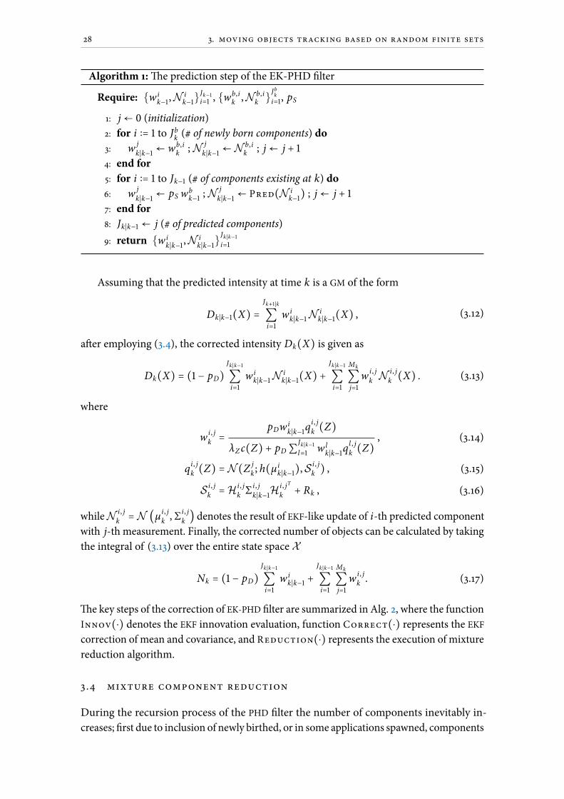
28 3. moving objects tracking based on random finite sets
Algorithm 1:e prediction step of the EK-PHD lter
Require: w ik−1,N
ik−1
Jk−1i=1 , w
b,ik,N b,i
kJbk
i=1, pS
1: j ← 0 (initialization)
2: for i ∶= 1 to Jbk(# of newly born components) do
3: wj
k∣k−1 ← wb,ik;N
j
k∣k−1 ← Nb,ik; j ← j + 1
4: end for5: for i ∶= 1 to Jk−1 (# of components existing at k) do6: w
j
k∣k−1 ← pS wbk−1 ;N
j
k∣k−1 ← Pred(Nik−1) ; j ← j + 1
7: end for8: Jk∣k−1 ← j (# of predicted components)
9: return w ik∣k−1,N
ik∣k−1
Jk∣k−1i=1
Assuming that the predicted intensity at time k is a GM of the form
Dk∣k−1(X) =
Jk+1∣k
∑i=1
w ik∣k−1N
ik∣k−1(X) , (3.12)
aer employing (3.4), the corrected intensity Dk(X) is given as
Dk(X) = (1 − pD)
Jk∣k−1
∑i=1
w ik∣k−1N
ik∣k−1(X) +
Jk∣k−1
∑i=1
Mk
∑j=1
wi , j
kN
i , j
k(X) . (3.13)
where
wi , j
k=
pDwik∣k−1q
i , j
k(Z)
λZc(Z) + pD∑Jk∣k−1l=1 w l
k∣k−1ql , j
k(Z)
, (3.14)
qi , j
k(Z) = N (Z
j
k; h(µ i
k∣k−1),Si , j
k) , (3.15)
Si , j
k= H
i , j
kΣi , j
k∣k−1Hi , jT
k+ Rk , (3.16)
whileNi , j
k= N (µ
i , j
k, Σ
i , j
k) denotes the result of EKF-like update of i-th predicted component
with j-th measurement. Finally, the corrected number of objects can be calculated by taking
the integral of (3.13) over the entire state space X
Nk = (1 − pD)
Jk∣k−1
∑i=1
w ik∣k−1 +
Jk∣k−1
∑i=1
Mk
∑j=1
wi , j
k. (3.17)
e key steps of the correction of EK-PHD lter are summarized in Alg. 2, where the function
Innov(⋅) denotes the EKF innovation evaluation, function Correct(⋅) represents the EKF
correction of mean and covariance, and Reduction(⋅) represents the execution of mixture
reduction algorithm.
3.4 mixture component reduction
During the recursion process of the PHD lter the number of components inevitably in-
creases; rst due to inclusion of newly birthed, or in some applications spawned, components

3.4. Mixture component reduction 29
Algorithm 2:e correction step of the EK-PHD lter
Require: w ik∣k−1,N
ik∣k−1
Jk∣k−1i=1 , Z
j
k∈ Zk
Mk
j=1 , pD
1: for i ∶= 1 to Jk∣k−1 (non-detected components) do2: w i
k← (1 − pD)w
ik∣k−1 ;N
ik← N i
k∣k−13: end for4: j ← 0 (measurement designator)
5: for all Zk ∈ Zk do6: j ← j + 1 , s j ← 0 (per measurement intensity)
7: for i ∶= 1 to Jk∣k−1 (detected components) do8: l ← i + j Jk∣k−1
9: [qi , j
k(Z)]← Innov(N i
k∣k−1, Zj
k)
10: w lk← pDw
ik∣k−1 q
i , j
k(Z), s j ← s j +w l
k
11: N lk← Correct(N i
k∣k−1, Zj
k)
12: end for13: for i ∶= 1 to Jk∣k−1 (re–weighting) do14: w
i+ j Jk∣k−1k
← wi+ j Jk∣k−1k
/(λZc(Z) + s j)
15: end for16: end for17: Jk ← ( j + 1)Jk∣k−1 (# of components existing at k)
18: w i ,Rk,N i ,R
kJRk
i=1 ← Reduction(wik,N i
kJki=1)
19: return w i ,Rk,N i ,R
kJRk
i=1
and second due to the nature of the PHD correction step. Namely, correcting the predicted
mixture by multiple measurements results in a geometrical increase in the component
number, which can be seen from (3.13). Given that, component number reduction schemes
are necessary [133]. Since this procedure is executed practically at each iteration, it should be
computationally modest, but still keep a reasonable level of accuracy. Reduction procedures
basically require three ingredients: (i) a component distance measure, (ii) a component
picking algorithm and (iii) component merging equations.
3.4.1 Component distance measure
e distance measure is a key ingredient in the reduction scheme and although numerous
distance measures between distributions exist, motivated by to practical and theoretical
aspects we concentrate on those appropriate for nite mixtures. Statistically and information
theoretically motivated distance measure is the Kullback–Leibler (KL) distance, also known
as the Kullback–Leibler divergence or the relative entropy [191], and dened as
DKL(p, q) = ∫X p(x) log(p(x)
q(x))dx .
It belongs to a wider class of distance measures called f-divergences or Ali-Silvey distances
[192]. Another statistical and information theoretical class of generalized distances are Rényi

30 3. moving objects tracking based on random finite sets
α-divergences [193] given by the following expression
D(α)R (p, q) =
1
α − 1log ∫X p(x)αq(x)1−αdx
and parametrized by real parameter α. In the limit α → 1, the Rényi α-divergence yield
the KL distance. Another well-established distance measure when α = 1/2 is called the
Bhattacharyya distance [194]. However, given the discussion presented in [195], we rely our
approaches on KL divergence and hence continue with further discussion on it.
3.4.2 Symmetrized Kullback-Leibler divergence
Furthermore, since the mixtures of distributions appearing in PHD are weighted, in order to
be used here, themeasure needs to be customized for weighted (unnormalized) distributions,
and additionally symmetrized. Since scaled symmetrized Rényi α-divergences neglect the
respective weights of components, for the purpose we consider the scaled symmetrized KL
distance [195].e distance measure between pdfs p and q, with their respective weights
wp and wq, is then given as [192]
DsKL(wpp,wqq) =1
2[wpDKL(p, q) +wqDKL(q, p)] +
1
2(wp −wq) log
wp
wq
. (3.18)
⊳ von-mises distributions. e equations for reducing the number of the compo-
nents in a mixture of von Mises distributions is presented in [195]. For the completeness of
the thesis we also provide the equations herein. Given two vMpdfs p(µp, κp) and q(µq , κq),
the KL distance is given as
DKL(p, q) = logI0(κq)
I0(κp)+ A(κp)(κp − κq cos(µp − µq)). (3.19)
where A(x) = I1(x)/I0(x) with Ip(x) as the the modied Bessel function of the rst kind
and of order p.
⊳ gaussian distributions. Given two Gaussian distribution pdfs, p(µp, Σp) and
q(µq , Σq), the KL distance is evaluated as
DKL(p, q) =1
2tr [(Σq)
−1Σp] − K + logR∣Σq∣
∣Σp∣+ (µq − µp)
T(Σq)−1(Σq − Σp), (3.20)
where tr( . ) and ∣ . ∣ designate matrix trace and determinant, respectively, while K is the
mean vector dimension.
3.4.3 Component picking strategy
With having dened the appropriate distancemeasure between the distributions we can now
employ the component picking algorithmwhich will tell us how to screen the whole mixture
and which components to pick for merging. Here we will consider two component picking
strategies interesting from the practical viewpoint, i.e., (i) Exhaustive pairwise [196], and (ii)

3.5. Metrics for evaluation 31
West’s [197] algorithms.e Exhaustive pairwise algorithm determines distances between
all components and merges the closes two, while West’s algorithm sorts the components
according to their respective weights, then nds and merges the component most similar to
the rst one.e resulting component is then inserted back to the mixture with respect to
its weight and the procedure is repeated until the desired number of components is reached.
3.4.4 Component merging equations
⊳ von-mises distributions. emerged vM component has the optimal parameters
in the KL sense obtained by following
µ∗ = arctanwpA(κp) sin µp +wqA(κq) sin µq
wpA(κp) cos µp +wqA(κq) cos µq
w∗A2(κ∗) =w2pA2(κp) + 2wpwqA(κp)A(κq) cos(µp − µq),
(3.21)
where w∗ = wi + w j, while w∗, µ∗ and κ∗ designate the parameters resulting from the
component merging procedure.
⊳ gaussian distributions. Given several Gaussian distributions the component
merging equations follow as [196]
w∗ =∑i
wi , µ∗ =1
w∗∑i
wiµi
Σ∗ =1
w∗∑i
wi [Σi + µi(µi)T] − µ∗(µ∗)T (3.22)
where w∗, µ∗ and Σ∗ designate the parameters resulting from the component merging.
Although (3.22) works for an arbitrary number of components, in our case we will always
merge just two components.
An example of the pseudocode of the merging algorithm using West’s picking strategy
and Gaussian distribution is given in Algorithm 3.
3.5 metrics for evaluation
e metric for evaluating the MOT algorithm needs to account for various appearances in
contrary to the single-object estimation where it is typically adequate to involve only a miss
distances as the Euclidean or Mahalanobis distance.e MOT performance metric needs to
involve measures of eectiveness (MoEs) such as missing tracks, false tracks, state estimation
error (position, velocity, heading), track initiation delay, track overshoot, track label swaps,
cardinality estimation, and is alongside strongly scenario and operation dependent.e
problem of choosing MoEs is questionable from two viewpoints; (i) how to choose the
relevant MoEs since it is fairly arbitrary and far from clear and (ii) which choice is adequate
from the theoretical point of view, since MoEs can be correlated.
Since the performance evaluation approaches are strongly application dependent, it
is hard to establish an adequate genericMOT evaluation framework that will embrace all
the previously introduced MoEs. For this reason, here we focus our overview on popular
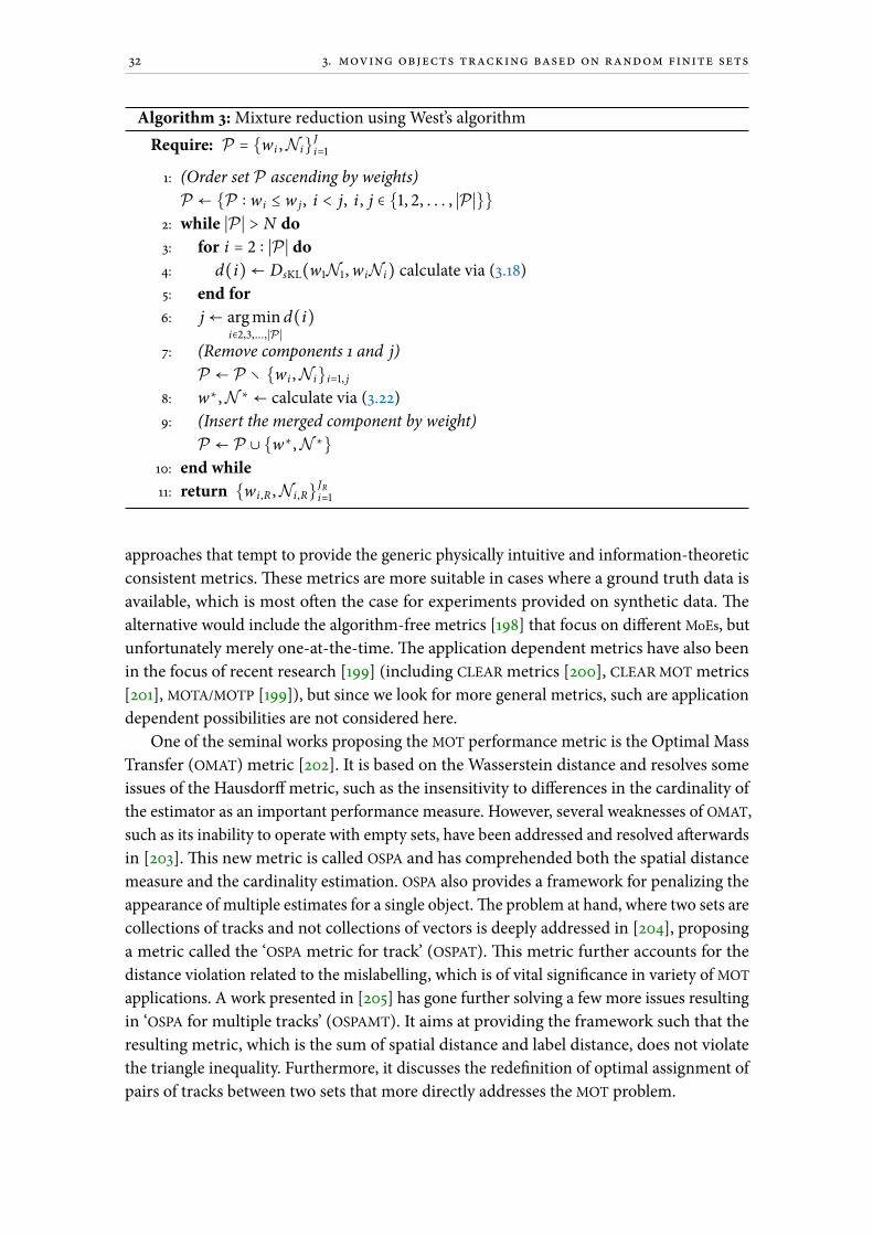
32 3. moving objects tracking based on random finite sets
Algorithm 3:Mixture reduction using West’s algorithmRequire: P = wi ,Ni
Ji=1
1: (Order set P ascending by weights)
P ← P ∶ wi ≤ w j, i < j, i , j ∈ 1, 2, . . . , ∣P ∣
2: while ∣P ∣ > N do3: for i = 2 ∶ ∣P ∣ do4: d(i)← DsKL(w1N1,wiNi) calculate via (3.18)
5: end for6: j ← argmin
i∈2,3,...,∣P ∣d(i)
7: (Remove components 1 and j)
P ← P ∖ wi ,Nii=1, j
8: w∗,N ∗ ← calculate via (3.22)
9: (Insert the merged component by weight)
P ← P ∪ w∗,N ∗
10: end while11: return wi ,R ,Ni ,R
JRi=1
approaches that tempt to provide the generic physically intuitive and information-theoretic
consistent metrics.ese metrics are more suitable in cases where a ground truth data is
available, which is most oen the case for experiments provided on synthetic data.e
alternative would include the algorithm-free metrics [198] that focus on dierent MoEs, but
unfortunately merely one-at-the-time.e application dependent metrics have also been
in the focus of recent research [199] (including CLEARmetrics [200], CLEARMOTmetrics
[201], MOTA/MOTP [199]), but since we look for more general metrics, such are application
dependent possibilities are not considered here.
One of the seminal works proposing the MOT performance metric is the Optimal Mass
Transfer (OMAT) metric [202]. It is based on the Wasserstein distance and resolves some
issues of the Hausdor metric, such as the insensitivity to dierences in the cardinality of
the estimator as an important performance measure. However, several weaknesses of OMAT,
such as its inability to operate with empty sets, have been addressed and resolved aerwards
in [203].is new metric is called OSPA and has comprehended both the spatial distance
measure and the cardinality estimation. OSPA also provides a framework for penalizing the
appearance of multiple estimates for a single object.e problem at hand, where two sets are
collections of tracks and not collections of vectors is deeply addressed in [204], proposing
a metric called the ‘OSPA metric for track’ (OSPAT).is metric further accounts for the
distance violation related to the mislabelling, which is of vital signicance in variety ofMOT
applications. A work presented in [205] has gone further solving a few more issues resulting
in ‘OSPA for multiple tracks’ (OSPAMT). It aims at providing the framework such that the
resulting metric, which is the sum of spatial distance and label distance, does not violate
the triangle inequality. Furthermore, it discusses the redenition of optimal assignment of
pairs of tracks between two sets that more directly addresses the MOT problem.

3.5. Metrics for evaluation 33
3.5.1 Metric denition
Let us dene a metric space (X ,D), where function D ∶ X ×X → R+ = [0,∞) is a metric
that satises the following three axioms for all X ,Y , Z ∈ X
1. Identity: D(X ,Y) = 0 if and only if X = Y .
2. Symmetry: D(X ,Y) = D(Y , X).
3. Triangle inequality: D(X ,Y) ≤ D(X , Z) +D(Z ,Y).
Upon that, the metric should be incorporating physical meaning and employing relevant
MoEs for MOT problem.
3.5.2 Optimal subpattern assignment
Let dc(x , y) ≜min(c, d(x , y)) be the distance between x , y ∈W ,W ∈ RN , cut o at c > 0.
Let further Πk be the set of permutations on 1, 2, ..., k for any k ∈ N = 1, 2, .... For
1 ≤ p <∞ and arbitrary subsets X = x1, ..., xn and Y = y1, ..., ym ofW , where m ≤ n,
m, n ∈ N0, dene the following
Dcp(X ,Y) ≜ (
1
n(min
π∈Πn
m
∑i=1
dc(xi , yπ(i))p + cp(n −m)))
1
p
(3.23)
and if m > n, Dcp(X ,Y) ≜ Dc
p(Y , X). Furthermore, for p →∞
Dc∞(X ,Y) ≜
⎧⎪⎪⎪⎨⎪⎪⎪⎩
minπ∈Πnmax1≤i≤n dc(xi , yπ(i)) if m = n
c if m ≠ n
. (3.24)
e functionDcp is called the OSPAmetric of order p and cut o c. It is interesting to mention
that OSPA satises the metric denition conditions, and a formal proof is given in [203].
OSPA is shown to eliminate some shortcomings of OMAT as follows:
• Consistency.e OSPAmetric penalizes relative dierences in cardinality by introduc-
ing an additive component on top of the average distance.
• Intuitive construction.e OSPA construction eliminates any element of arbitrariness
by providing an objective and intuitively reasonable criterion for the assignment,
while at the same time observing the metric axioms.
• Geometry dependence. For a given c and p,Dcp distance does not substantially depend
on the size of the ground truth pattern.
• Cardinality zero.e OSPAmetric is dened between any two point patterns.
• Compatibility with mathematical theory.e OSPA generates the vague topology on
the space of nite point patterns on W, which is the standard topology used in point
process theory.

34 3. moving objects tracking based on random finite sets
e OSPAmetric can be computed eciently by using the Hungarian or Munkres methods
for optimal assignment, which is by theoretical complexity just as good as OMAT.
e combined localization and cardinality error represented by theOSPAmetric conceals
the reason for the large distance, whence the metric may be split up into a localization and
cardinality error
Dc,locp (X ,Y) ≜ (
1
nminπ∈Πn
m
∑i=1
dc(xi , yπ(i))p)
1
p
(3.25)
Dc,cardp (X ,Y) ≜ (
1
ncp(n −m))
1
p
. (3.26)
Although this is not a metric on the space of nite subsets any more, it can be interpreted
as error measures due to localization only and cardinality only (penalized at maximal
distance).
For object tracking, however, we oen require a metric on the space of nite sets of
tracks, where a track has been dened as a labeled temporal sequence. For such requirements
the OSPAmetric does not provide the full support, hence its extensions have come to the
focus of consideration for the MOT research.is extensions need to be directed towards
incorporation of information about track continuity or switching of track labels. However,
since we do not consider the labeling problem specically, we chose original OSPA as an
adequate metric for our applications of interest.
4e main scientic contributions of the thesis
The four original contributions of the thesis essentially revolve about probabilistic
methods in estimation and multiple moving objects tracking relying on the models of
uncertainty respecting the pertaining geometry of the system described using Lie groups.
e rst and the last contributions of the thesis deal with the problem of multiple moving
objects tracking when the state arises on non-Euclidean manifold [Pub1, Pub7, Pub8].e
second and third contributions deal with the problem of estimation in the space of the
special Euclidean group [Pub2, Pub3, Pub4, Pub5], the extended information lter tailored
for the geometry of matrix Lie groups [Pub6].e discussion on contributions follows in
the sequel.
#1 Method for multiple moving objects tracking on the unit sphere based on the vonMises
distribution and the random nite sets
e state of the system can generally appear to be non-Euclidean which with all the usual
issues makes the MOT problem even more complex. In particular, most of the MOT ap-
proaches somehow rely on the Bayesian recursion and although there is nothing intrinsic
in this concept, it is a real challenge to develop a computationally tractable solution for
the non-Euclidean geometries. Firstly, it is challenging to solve the Chapman–Kolmogorov
equation (Bayesian prediction) in closed form, such that it results with the same type of
distribution as the beginning one. Secondly, given a distribution associated to a predicted
value and employing a measurement likelihood, it is challenging evaluate the Bayes rule
(Bayesian update) hopefully again obtaining the same type of distribution.
e vM is an example of directional distribution dened on the unit circle and as such
captures the geometry of the state space in a global manner. Given two vMs, the convolution
integral of Bayesian prediction does have an exact solution, but the result is not a vM
distribution. However, the resulting distribution can be well-approximated with another
vM based on circular moment matching.e update step on the other hand exhibits a vM
distribution without approximations.
e rst contribution deals with the MOT task on the unit circle, based on the PHD
lter which represents an approximation of the optimal multi-object Bayes lter developed
upon the theory of RFS. We particularly derive a closed-form recursion of the PHD lter
yielding a nite vMmixture approximation (vM-PHD) [Pub1].e vM-PHD is compared to
the GM-PHD on a synthetic dataset of 100 randomly generated multi-object scenarios and
35
36 4. the main scientific contributions of the thesis
on the real-world PETS2009 dataset, and achieved respectively a decrease of 10.5% and 2.8%
in the OSPAmetric.
#2 Method for moving object tracking in the space of the special Euclidean group based on
the extended Kalman lter on Lie groups
Lie groups are natural ambient spaces for description of the dynamics of rigid body me-
chanical systems. A common state space representation of a rigid body object pose is the
one using semi-direct product of the SO group for orientation and the Euclidean trans-
lation vector, yielding the 2D and 3D counterparts denoted SE(2) and SE(3). Although
development of a convenient distribution dened directly on an SE group represents a
signicant research goal, so far there does not exist such solution suitable for employment
in the standard Bayesian framework. Hence, the global approach used for development of
the rst contribution is not possible when the underlying state space is SE rather than the
simple unit circle.e CGD is a distribution with parameters which partially combine both
worlds, including a mean value dened on a Lie group and the uncertainty described with
the Gaussian variance in the Euclidean world arising as a tangent space at the mean value.
e research respecting this contribution begins with the consideration of special orthog-
onal group SO(2) and emulation of the constant acceleration model used within LG-EKF,
and was applied for the problem of speaker tracking with a microphone array [Pub2]. An
important concluding remark of [Pub2] is that application of SO(2) group within LG-EKF
yields the same result as heuristically wrapping the angular variable within the EKF frame-
work which is due to commutativity of this group. Next, we continued with the research
on pose estimation employing the SE(2) group and emulating the constant velocity model
used within LG-EKF suitable for tracking of an omnidirectional motion [Pub3]. By using
this modeling approach we inherently account for the nature of coupling between the
rotation and translation parts of SE group. In accordance, association of uncertainty to
an SE(2) group exhibits more exibility, i.e., supports the banana shaped forms of un-
certainty contours, rather than only elliptical contours. When compared to the classical
constant velocity KF/EKF in a omnidirectional motion tracking application, the proposed
lter outperforms the classical approach for a wide range of acceleration change intensities.
Finally, we developed the constant acceleration model within LG-EKF framework for the
full body human motion estimation employing SO(2), SO(3) and SE(3) groups, by relying
on 3D marker position measurements in [Pub4] and inertial measurement units in [Pub5].
In both cases we provided derivation of the LG-EKF recursion for the articulated motion
estimation. Detailed derivation of accelerometer based update is given in supplementary
material [*Pub5]. We compared the performance of the proposed approaches with the Euler
angles-based EKF, and showed that these algorithms achieve better performance in both
simulations and real-world experiments.
#3 Extended information Kalman lter for state estimation on matrix Lie groups
e IF is the dual of the classicalKF, and is the subject of the same assumptions underlying the
KF. Whereas the KF is represented by mean and covariance, the IF relies on the parametriza-
tion consisting of an information matrix and an information vector. Probably the simplest

37
advantage of the IF is recognized in the update step when number of measurements is larger
than state space size, while the opposite applies for the KF.
Although IFs have been successfully applied in a number of applications facing large
number of measurements, features or demanding a decentralized lter form, a quite promi-
nent example of an application where the need arises for computational benets of the
IF is SLAM. Additionally, in SLAM applications the need arises for the geometric accuracy
of Lie groups as well.e earliest SLAM solutions were based on the EKF, which turned
out being inadequate approach due to limitations in maps size, hence EIF soon became
widely accepted for SLAM and reached its zenith with SEIF and ESDSF. However, the pose in
SLAM usually conforms the variables arising on SE(3) groups, and therefore in some recent
solutions it was determined that the approximation in state space geometry represents a
signicant cause of error, and the new approaches accounting for this geometry were devel-
oped. However, these SLAM solutions exclusively relied on graph optimization approaches
since no ltering approaches in the form of IF on Lie groups were available.
As a third contribution, the extended information lter on matrix Lie groups (LG-EIF)
is proposed [Pub6]. We provided the theoretical development of the LG-EIF recursion
equations and the applicability of the proposed approach is demonstrated on a rigid body
attitude tracking problem with multiple sensors. We particularly compared the proposed LG-
EIF to an EIF based on Euler angles, and analyzed its computational complexity regarding the
multisensor update with respect to the LG-EKF.e results showed that the proposed lter
achieves higher performance consistency and smaller error by tracking the state directly on
the Lie group and that it keeps smaller computational complexity of the information form
with respect to large number of measurements.
#4 Method for multiple moving objects tracking on Lie Groups based on the concentrated
Gaussian distribution and the random nite sets
While the rst contribution deals with a global approach to MOT problem [Pub1] as a long-
term goal for nearly any non-Euclidean probabilistic application, many MOT applications
deal with objects and measurements whose state space is non-Euclidean and is oen more
complex than a simple unit circle. Furthermore, both (i) diverse traditional engineering
disciplines (intelligence, surveillance, air trac control, resident space objects tracking)
and (ii) some modern engineering elds (autonomous systems and robotics) deal with
the objects described with their pose including the orientation variables, which instantly
denes their non-Euclidean nature. Many of those applications can successfully rely on Lie
group representation of the tracked objects, particularly employing either SE group, and
the ltering approach presented as part of the second contribution. Now, when put into
MOT context several additional questions arises.
As the rst part of this contributionwe proposed to use a solution based on the JIPDAlter,
which was shown to be derived within the RFS framework (as part of the family of JPDA-like
approaches). OurMOT solution uses a modied JIPDA lter suitable for operation on matrix
Lie groups [Pub7]. In particular, the probabilities of each event of the lter do not reason
over the space of the variable itself, but rather in the tangent Lie algebra space associated to
the predicted state of some considered object. Only aer the innovation vector is determined,

38 4. the main scientific contributions of the thesis
we use the addition operator, which on the group appears as matrix multiplication, and
hence update the considered object state.e proposed approach is tested using a real-world
dataset collected in urban trac scenarios with the multisensor setup consisting of a radar
and a stereo camera mounted on top of a vehicle.e uncertainties of sensors were modeled
in polar coordinates on Lie Groups, while the states were represented with SE(2) groups.
As the second part of this contribution we proposed a mixture approximation of the
PHD lter tailored for matrix Lie groups, denoted LG-PHD. It is based on the mixture of
CGDs, and as any PHD lter, it inherently faces the problem of an ever increasing number
of mixture components. For this purpose, the growth of components must be controlled
by approximating the original mixture with the mixture of a reduced size. As part of the
thesis we propose a reduction approach for mixture of CGDs. is entails appropriate
reparametrization of CGD parameters to compute the KL divergence, and pick and merge
the CGDmixture components. Since reparametrization of two dierent components requires
choosing the appropriate tangent space, we also provide an extensive analysis on the choice
thereof. Detailed derivation of the LG-PHD is given in supplementary material [*Pub8]. We
compared the performance of LG-PHD lters relying on dierent choices of tangent space
using the OSPAmetric.
5Conclusions and future work
Autonomous navigation represents a highly disruptive technology that will certainly
change the way people live and behave, and transform the work practices raising the
eciency and safety in dierent types of services. A problem of multiple moving objects
tracking has been the focus of dierent research studies for several decades and represents an
essential feature in the autonomous navigation task. Still, the ‘tracking research community’
in majority of applications approach this problem by neglecting the non-Euclidean state
space geometry of typically tracked objects, and usually assume the underlying statistics
follow a ‘classical’ Gaussian distribution.
5.1 the main conclusions of the thesis
is thesis considers the MOT task by emphasizing the problem of the geometry of the
state space associated to tracked objects and employed measurements, especially from the
viewpoint of uncertainty description.e problem of associating uncertainty to dierent
non-Euclidean geometries is herein considered in the twofold manner; rst by using the
statistics which globally captures geometry, and second by using an uncertainty description
which locally accounts for it. However, the estimation approaches capable of accounting for
a global geometry of the non-Euclidean ambient space represent an ultimate goal.
One part of the thesis dealt with the MOT problem when the underlying state and mea-
surement space was a direction/a unit circle.is approach was based on the vM distribution
which is dened directly on the space of interest. Since given two vMs, the convolution
integral of Bayesian prediction can be approximated with another vM, and since Bayesian
update given two vMs results explicitly with another vM, we could proceed with develop-
ment of the MOT solution.e main challenge when applying this distribution in a MOT
application was to account for many additional statistical appearances that do not exist in an
estimation-only task.e thesis started by developing a method for directional MOT appli-
cation and derivation of a novel mixture approximation of the PHD lter tailored specically
for the system on the unit circle (vM-PHD).e resulting lter required some principled
approximations to achieve closed-form and ensure numerical stability.e conclusion
respecting the optimal subpattern assignment metric is that globally accounting for the
circular geometry of the state space can signicantly boost accuracy of MOT applications
arising on this type of manifold.
Although the global uncertainty description seems to be attractive, its practical applica-
39
40 5. conclusions and future work
bility is oen very limited. For this purpose, next part of the thesis dealt with the description
of dynamics of a rigid body mechanical system representing its pose with the special Eu-
clidean group (SE) and orientation with the special orthogonal group (SO).e uncertainty
was associated to these Lie groups relying on the concept of CGD, parametrized with the
mean value on the group and the Gaussian variance in the Euclidean space obtained as a
tangent space at the mean value. As part of this research we studied several models on Lie
groups employed in dierent applications, including alternatives to Euclidean space based
constant velocity and constant acceleration models but this time arising on Lie groups.
Before proceeding with dierent motion models, as probably the simplest Lie group
representative, we studied the SO(2) group by analyzing it in the context of the mathemati-
cally grounded framework of LG-EKF. We have shown that the similar result is obtained by
heuristically wrapping the EKF.is result did not seem unexpected given that SO(2) is
abelian, i.e., commutative, but gives an interesting theoretical perspective on estimation
and tracking with the heuristically modied EKF. On the other hand, it was shown that
employment of SE(2) group in the case when rotational dynamics exists can signicantly
boost the quality of estimation. In particular, when both dynamics in translation and ro-
tation induce the system it is more appropriate to use a constant velocity model on SE(2)
than the EKF based constant velocity and turn rate model or the linear KF based constant
velocity model. As part of the thesis we further combined SE(3), SO(2) and SO(3) Lie
group representatives in a novel algorithms for the full body human motion estimation
based on (i) body worn marker position measurements and (ii) inertial measurement units.
e human joints were described with SO(2) or SO(3) groups depending on the number of
dofs, while the initial joint representing the connection of the body with the world reference
frame was represented with an SE(3).e motion was assumed to follow the constant
acceleration model within the LG-EKF framework. We evaluated the performance of the
proposed methods on both simulation and real-world motion capture data, comparing it
with the Euler angles-based EKF, and additionally with the commercial soware Vicon IK
when dealing with marker measurements. It was shown that the LG-EKF-based solutions
improve estimation for highly dynamic motions and are not aected by gimbal lock.
Next, the thesis deals with the problem of estimation on matrix Lie groups when it may
be adequate to apply an information form. Given the advantages of the IF form and dealing
with ltering on Lie groups, a natural question on casting the LG-EKF in the information
form while keeping its additivity and computational advantages arises. We proposed a
new state estimation method which embedded the LG-EKF with an EIF form for non-linear
systems, thus endowing the lter with the information forms advantages, while keeping
the accuracy of the LG-EKF for stochastic inference.e lter was tested on the problem of
rigid body attitude tracking assuming a constant velocity model with multiple sensors.e
results have shown that the lter can accurately track the attitude and exhibits lower RMSE
with respect to the Euler angles based EIF, and keeps the computational advantages of the
update step with respect to the LG-EKF.
Finally, two solutions to the MOT problem for the system arising on Lie groups were
proposed in the thesis.e rst one was based on the JIPDA lter, and modied such that
it is able to operate on Lie groups, hence reasoning about probabilities and the combined
innovation vector in the tangential Lie algebra space.e proposed MOT approach was

5.2. Further research directions 41
tested in an advanced driver assistance system application on a real-world dataset collected
using a radar and a stereo camera mounted on top of a vehicle.e stereo camera estimated
relative displacement of the vehicle, using stereo visual odometry, generating measurements
as cluster centers of optical ow vectors not conforming to the estimated motion.e radar
directly reported its measurements to the lter, thus complementing the stereo camera
measurements. Both radar and stereo camera were modeled as polar sensors, while the
vehicle state resided on SE(2) group, thus enabling more reliable model of uncertainties
supporting the banana-shaped contours, in contrast to elliptical uncertainty contours given
by the ‘classical’ Gaussian distribution.
We have also developed the PHD lter tailored for the topology of Lie groups (LG-PHD),
and studied the problem of manipulating the size of the mixture of CGD components. For
this purpose, the reduction scheme for mixture of CGD components, including evaluation
of the KL divergence, as well as component picking and merging scheme are considered.
5.2 further research directions
e thesis includes some theoretical results that could possibly be further applied in dierent
applications. One such example is the LG-EIFwhich represents an estimation framework that
could be applied for further development of ltering based SLAM approaches. In particular,
the ltering based SLAM solutions reached its zenith with appearances of sparsication
approaches applied over some original EIF implementations, resulting with sparse EIF and
exactly sparse delayed-state lters. Soon aer, optimization based SLAM solutions prevailed
over the ltering based solutions since they dominated in performance over a wider range
of applications.e herein presented LG-EIF could represent a basis for development of a
new lter-based back-end for solving SLAM.
e thesis deals with the global estimation approach if it was possible to have a distribu-
tion closed under convolution and Bayes rule. Otherwise, it relies on the approximations
developed upon the concept of concentrated Gaussian distribution. Unfortunately, subtle
global distributions characterized with useful properties, such as an analytic solution to
the Chapman-Kolmogorov convolution integral or closed form under application of the
Bayes rule, are generally uncommon. For this purpose, further research direction in terms
of theoretical aspects may point towards development of some better approximations of Lie
group random variables rather then relying on the concept of CGD.
Considering theMOT applications, it is important to note that the question of an optimal
solution to a complexMOT system is still open, while the key goal of the ongoing research is to
develop near-optimal, scalable and numerically ecient algorithms. Furthermore, alongside
the traditional elds whereMOTwas applied, some new large-scale real-world problems such
as space objects tracking and giga-pixel video surveillance system, have come in the research
focus.ese problems usually include thousands of tracked objects and appearance of some
additional issues that were neglected in this thesis, such as extended objects appearance,
multiple source measurements, coalescence problem, etc. Additionally, although MOT eld
is experiencing a rapid development relying on a large scientic community working on new
algorithms, an interesting contribution to the community would be providing an exhaustive
comparison of dierent MOT approaches since the research in this area is limited.

6List of publications
Pub1 I. Marković, J. Ćesić and I. Petrović. Von Mises Mixture PHD Filter. IEEE Signal
Processing Letters, 22(12):2229–2233, 2015, IF: 1.661 (Q2).
Pub2 I. Marković, J. Ćesić and I. Petrović. On wrapping the Kalman lter and estimating
with the SO(2) group. International Conference on Information Fusion (FUSION).
Heidelberg, Germany, 2245–2250, 2016.
Pub3 J.Ćesić, I. Marković and I. Petrović. Moving object tracking employing rigid bodymo-
tion on matrix Lie groups. International Conference on Information Fusion (FUSION).
Heidelberg, Germany, 2109–2115, 2016.
Pub4 J. Ćesić, V. Joukov, I. Petrović and D. Kulić. Full Body Human Motion Estimation
on Lie Groups Using 3D Marker Position Measurements. IEEE-RAS International
Conference on Humanoid Robotics (Humanoids). Cancun, Mexico, 826–833, 2016.
Pub5 V. Joukov, J. Ćesić, K. Westermann, I. Marković, D. Kulić and I. Petrović. Human
motion estimation on Lie groups using IMUmeasurements. IEEE/RSJ International
Conference on Intelligent Robots and Systems (IROS) Vancouver, Canada, 1965–1972,
2017.
*Pub5 Supplementary material to Pub5
Pub6 J. Ćesić, I. Marković, M. Bukal and I. Petrović. Extended information lter on matrix
Lie groups. Automatica, 53(9):226–234, 2017, IF: 5.451 (Q1).
Pub7 J. Ćesić, I. Marković, I. Cvišić and I. Petrović. Radar and stereo vision fusion for
multitarget tracking on the special Euclidean group. Robotics and autonomous systems,
83:338–348, 2016, IF: 1.950 (Q2).
Pub8 J. Ćesić, I. Marković and I. Petrović. Mixture Reduction on Matrix Lie Groups. IEEE
Signal Processing Letters, 24(11):1719–1723, 2017, IF: 2.528 (Q2).
*Pub8 Supplementary material to Pub8
42

7Author’s contribution to publications
The results presented in this thesis are based on the research carried out during the
period of 2013 − 2017 in the Laboratory for autonomous systems and mobile robotics
(LAMOR) headed by Professor Ivan Petrović, at the University of Zagreb, Faculty of Electrical
Engineering and Computing, Croatia, as a part of three research projects: including:
• [2013 − 2015] VISTA - Computer Vision Innovations for Safe Trac (IPA2007/HR/
16IPO/001-040514) which was nancially partially supported by the European Union
from the European Regional Development Fund.
• [2015 − 2016] FER-KIET - Advanced Technologies in Power Plants and Rail Vehicles
(RC.2.2.08-0015) which was as well nancially supported by the European Union
from the European Regional Development Fund.
• [2016−2017] cloudSLAM - Cooperative cloud based simultaneous localization andmap-
ping in dynamic environments (25/15) which was funded by the Unityrough Knowl-
edge Fund (UKF).
A part of the thesis also includes the research carried out at the Adaptive systems laboratory
headed by Professor Dana Kulić, at the University of Waterloo, Canada, who was actively
participating as partner in the cloudSLAM project.
e thesis includes eight publications written in collaboration with co-authors of the
published papers.e author’s contribution to each paper consists of the text writing, the
soware implementation, performing the required simulations and experiments, and results
analysis and presentation.
Pub1 In the paper entitled Von Mises Mixture PHD Filter the author proposed a novel
mixture approximation of the PHD lter tailored specically for the topology of an
MOT system on the unit circle relying on the vM distribution, which arises whenever
the state and the sensor measurements are circular.e author has implemented the
newly proposed algorithm in Matlab and analyzed the performance of the proposed
lter comparing it with the GM-PHD on a synthetic dataset of 100 randomly generated
multi-object scenarios with respect to the optimal subpattern assignment metric.
Pub2 In the paper entitled On wrapping the Kalman lter and estimating with the SO(2)
group the author analyzes the LG-EKF for directional tracking of moving object in
43
44 7. author ’s contribution to publications
2D assuming the constant angular acceleration model on the Lie groups including
SO(2) (orientation) and Euclidean variables (velocity and acceleration).e author
particularly shows that LG-EKF lter derivation based on themathematically grounded
framework of ltering on Lie groups (including SO(2) group) yields the same result
as heuristically wrapping the angular variables within the EKF framework.e author
has applied the proposed lter for a real-world speaker tracking with a microphone
array using the implementation under the Robotic Operating System (ROS), while the
accuracy was evaluated with ground truth data obtained by a motion capture system.
Pub3 In the paper entitledMoving object tracking employing rigid body motion on matrix
Lie groups the author proposed a novel method for estimating rigid body motion by
modeling the object state using special Euclidean group SE(2) and employing the
LG-EKF constant velocity model.e performance of the lter is then analyzed using
Matlab implementation on a large number of synthetic trajectories and compared
with (i) the EKF constant velocity and turn rate model and (ii) the linear KF constant
velocity model.
Pub4 In the paper entitled Full Body Human Motion Estimation on Lie Groups Using 3D
Marker PositionMeasurements, in collaborationwith co-authors, the author proposed
a new algorithm for full body human motion estimation using 3D marker position
measurements. For this purpose, the LG-EKF is used for stochastic inference on SO(2),
SO(3) and SE(3) groups.e motion prediction follows the constant acceleration
model, while the update and observation equations are derived for positional mea-
surements, accounting for the kinematic chain.e performance of the lter was
evaluated in both simulation and on real-world motion capture data, comparing it
with the Euler angles based EKF.
Pub5 In the paper entitled Human motion estimation on Lie groups using IMU measure-
ments, in collaboration with co-authors, the author proposed a new algorithm for full
body human motion estimation using inertial measurement units.e LG-EKF was
employed for an arbitrary chain conguration consisting of SO(2) or SO(3) joints.
e motion prediction follows the constant acceleration model, while the update was
derived for gyro and accelerometer measurements, accounting for inuence of the
kinematic chain.e performance of the lter was evaluated in simulations and on
real-world data, comparing it with the Euler angles based EKF.
*Pub5 is material provides a detailed derivation of accelerometer update within the LG-EKF
framework employing an arbitrary kinematic chain, thus serving as a supplementary
material to [Pub5].
Pub6 In the paper entitled Extended information lter on matrix Lie groups the author
proposed a new state estimation algorithm called the extended information lter on
Lie groups (LG-EIF)e paper presents the theoretical development of the LG-EIF
recursion equations and the applicability of the proposed approach is demonstrated
on a rigid body attitude tracking problem with multiple sensors, comparing the

45
proposed LG-EIF to an EIF based on Euler angles, and analyzing its computational
complexity with respect to the LG-EKF.
Pub7 In the paper entitled Radar and stereo vision fusion for multitarget tracking on the
special Euclidean group the author uses a combination of a radar and a stereo vision
system to perform the MOT task, by relying on the measurements and object states
described using Lie groups.e paper also presents the adaptation of the JIPDA lter
for MOT application on matrix Lie groups.e implementation in ROS was used for
testing the algorithm on a real-world dataset collected with the describedmulti-sensor
setup in urban trac scenarios.
Pub8 In the paper entitledMixture Reduction on Matrix Lie Groups the author proposes
a mixture reduction approach for CGDs dened on matrix Lie groups.is entails
appropriate reparametrization of CGD parameters to compute the KL divergence, pick
andmerge the mixture components.e author also describes anMOT lter, i.e., prob-
ability hypothesis density lter on matrix Lie groups (LG-PHD) with approximation
based on a nite mixture of CGDs, and uses it as a study example for the proposed
mixture reduction method.
*Pub8 is material provides a more detailed overview of derivation of LG-PHD, thus serving
as a supplementary material to [Pub8].
bibliography
[1] Sebastianrun, Wolfram Burgard, and Dieter Fox. Probabilistic Robotics. MIT
Press, 2006.
[2] Mahendra Mallick, Ba-Ngu Vo,ia Kirubarajan, and Sanjeev Arulampalam. Intro-
duction to the issue on multitarget tracking. IEEE Journal of Selected Topics in Signal
Processing, 7(3):373–375, 2013.
[3] Ronald P. S. Mahler. Multitarget bayes ltering via rst-order multitarget moments.
IEEE Transactions on Aerospace and Electronic Systems, 39(4):1152–1178, 2003.
[4] I. R. Goodman, Ronald P. Mahler, and Hung T. Nguyen. Mathematics of Data Fusion.
Kluwer Academic Publishers, Norwell, MA, USA, 1997.
[5] R. E. Kalman. A New Approach to Linear Filtering and Prediction Problems. Journal
of Basic Engineering, 82(1):35, 1960.
[6] P.-A. Absil, R. Mahony, and R. Sepulchre. Optimization Algorithms on Matrix Mani-
folds. Princeton University Press, Princeton, 2008.
[7] K.V. Mardia and P.E. Jupp. Directional Statistics. Wiley Series in Probability and
Statistics. John Wiley & Sons, Inc., 1999.
[8] Richard von Mises. Uber die ‘Ganzzahligkeit’ der Atomgewicht und Verwandte
Fragen. Physikalische Zeitschri, 19:490–500, 1918.
[9] Andrew W Long, Kevin C Wolfe, Michael J Mashner, and Gregory S Chirikjian. e
BananaDistribution is Gaussian : A Localization Studywith Exponential Coordinates.
In Robotics: Science and Systems (RSS), Sydney, Australia, 2012.
[10] Timothy D. Barfoot and Paul T. Furgale. Associating Uncertainty With ree-
Dimensional Poses for Use in Estimation Problems. IEEE Transactions on Robotics,
30(3):679–693, jun 2014.
[11] Gregory S. Chirikjian. StochasticModels, Informationeory, and LieGroups, Volume
1: Classical Results and Geometric Methods. Springer, 2012.
[12] Simo Srkk. Bayesian Filtering and Smoothing. Cambridge University Press, New
York, NY, USA, 2013.
46

bibliography 47
[13] R. E. Kalman and R. S. Bucy. New results in linear ltering and prediction theory.
Journal of Basic Engineering, 83(1):95–108, 1961.
[14] Mohinder S. Grewal and Angus P. Andrews. Kalman ltering: theory and practice.
John Wiley & Sons, Inc., second edition, 2001.
[15] Brian D. O. Anderson and John B Moore. Optimal Filtering. Prantice Hall, Inc.,
Englewood Clis, New Jersey 07632, 1979.
[16] A.H. Jazwinski. Stochastic Processes and Filteringeory. Dover Books on Electrical
Engineering Series. Dover Publications, 2007.
[17] Simon Julier and Jerey Uhlmann. Unscented Filtering and Non Linear Estimation.
Proceedings of the IEEE, 92(3):401–422, 2004.
[18] Eric A. Wan and Rudolph Van Der Merwe. e Unscented Kalman Filter for Non-
linear Estimation. In Adaptive Systems for Signal Processing, Communications, and
Control Symposium (AS-SPCC), pages 153–158, Lake Louise, Alta, 2000. IEEE.
[19] Fredrik Gustafsson and Gustaf Hendeby. Some relations between extended and
unscented Kalman lters. IEEE Transactions on Signal Processing, 60(2):545–555,
2012.
[20] I. Arasaratnam and S. Haykin. Cubature Kalman Filters. IEEE Transactions on
Automatic Control, 54(6):1254–1269, jun 2009.
[21] Bin Jia, Ming Xin, and Yang Cheng. e high-degree cubature Kalman lter. In
Conference on Decision and Control (CDC), number 2, pages 4095–4100. IEEE, dec
2012.
[22] K. Ito and K. Xiong. Gaussian lters for nonlinear ltering problems. IEEE Transac-
tions on Automatic Control, 45(5):910–927, may 2000.
[23] Ienkaran Arasaratnam, Simon Haykin, and Robert J Elliott. Discrete-Time Nonlinear
Filtering Algorithms Using Gauss – Hermite Quadrature. Proceedings of the IEEE,
95(5):953–977, 2007.
[24] S. Arulampalam, S. Maskell, N. Gordon, and T. Clapp. A tutorial on particle lters
for online nonlinear/non-Gaussian Bayesian tracking. IEEE Transactions on Signal
Processing, 50(2):174–188, 2002.
[25] D. Alspach and H. Sorenson. Nonlinear bayesian estimation using gaussian sum
approximations. IEEE Transactions on Automatic Control, 17(4):439–448, 1972.
[26] Rong Chen and Jun S. Liu. Mixture Kalman lters. Journal of the Royal Statistical
Society: Series B (Statistical Methodology), 62(3):493–508, 2000.
[27] P S Maybeck. Stochastic models, estimation, and control, volume Vol 1. Academic
Press, Inc., 1979.

48 bibliography
[28] B. Grocholsky, A. Makarenko, and H. Durrant-Whyte. Information-theoretic coordi-
nated control of multiple sensor platforms. In International Conference on Robotics
and Automation (ICRA), volume 1, pages 1521–1526. IEEE, 2003.
[29] TomVercauteren and XiaodongWang. Decentralized sigma-point information lters
for target tracking in collaborative sensor networks. IEEE Transactions on Signal
Processing, 53(8):2997–3009, 2005.
[30] Mark E. Campbell and William W. Whitacre. Cooperative tracking using vision
measurements on SeaScan UAVs. IEEE Transactions on Control Systems Technology,
15(4):613–626, 2007.
[31] Guoliang Liu, Florentin Wörgötter, and Irene Markelić. Square-Root Sigma-Point
Information Filtering. IEEE Transactions on Automatic Control, 57(11):2945–2950,
2012.
[32] Shiyuan Wang, Jiuchao Feng, and Chi K. Tse. A class of stable square-root nonlinear
information lters. IEEE Transactions on Automatic Control, 59(7):1893–1898, 2014.
[33] Deok-Jin Lee. Nonlinear Estimation and Multiple Sensor Fusion Using Unscented
Information Filtering. IEEE Signal Processing Letters, 15(2):861–864, 2008.
[34] Sebastianrun, Yufeng Liu, Daphne Koller, Andrew Y. Ng, Zoubin Ghahramani,
and Hugh Durrant-Whyte. Simultaneous Localization and Mapping with Sparse
Extended Information Filters. e International Journal of Robotics Research, 23(7-
8):693–716, 2004.
[35] Ryan M. Eustice, Hanumant Singh, and John J. Leonard. Exactly sparse delayed-state
lters for View-Based SLAM. IEEE Transactions on Robotics, 22(6):1100–1114, 2006.
[36] Volkan Cevher, Rajbabu Velmurugan, and James H. McClellan. Acoustic multitarget
tracking using direction-of-arrival batches. IEEE Transactions on Signal Processing,
55(6):2810–2825, 2007.
[37] Johannes Traa and Paris Smaragdis. AWrapped Kalman Filter for Azimuthal Speaker
Tracking. IEEE Signal Processing Letters, 20(12):1257–1260, 2013.
[38] Hagit Shatkay and Leslie Pack Kaelbling. Learning geometrically-constrained hid-
den Markov models for robot navigation: bridging the topological-geometrical gap.
Journal of Articial Intelligence Research, 16(1):167–207, 2002.
[39] Nicholas Roy, Georey Gordon, and Sebastianrun. Finding approximate POMDP
solutions through belief compression. Journal of Articial Intelligence Research, 23:1–
40, 2005.
[40] Ivan Marković and Ivan Petrović. Speaker Localization and Tracking in Mobile
Robot Environment Using a Microphone Array. Robotics and Autonomous Systems,
58(11):1185–1196, 2010.

bibliography 49
[41] Ivan Marković and Ivan Petrović. Applying von Mises Distribution to Microphone
Array Probabilistic Sensor Modelling. In Robotics (ISR), 2010 41st International Sym-
posium on and 2010 6th German Conference on Robotics (ROBOTIK), pages 1 – 7,
Munich, Germany, 2010. VDE.
[42] Ivan Marković and Ivan Petrović. Bearing-Only Tracking with a Mixture of von
Mises Distributions. In International Conference on Intelligent Robots and Systems
(IROS), pages 707 – 712, Vilamoura, Portugal, 2012. IEEE.
[43] Ivan Markovic, Alban Portello, Patrick Danes, Ivan Petrovic, and Sylvain Argentieri.
Active speaker localization with circular likelihoods and bootstrap ltering. In
International Conference on Intelligent Robots and Systems (IROS), pages 2914–2920.
IEEE/RSJ, 2013.
[44] Simone Calderara, Andrea Prati, and Rita Cucchiara. Mixtures of von Mises Dis-
tributions for People Trajectory Shape Analysis. IEEE Transactions on Circuits and
Systems for Video Technology, 21(4):457–471, 2011.
[45] David Crouse. Maximum Likelihood Postdetection Radar Ambiguity Resolution.
IEEE Transactions on Aerospace and Electronic Systems, 50(3):1876–1883, 2014.
[46] Yang Yi and Haohui Xu. Hierarchical data association framework with occlusion
handling for multiple targets tracking. IEEE Signal Processing Letters, 21(3):288–291,
2014.
[47] N. I. I. Fisher. Statistical Analysis of Circular Data. Cambridge University Press, 1993.
[48] Ivan Marković, François Chaumette, and Ivan. Moving object detection , tracking
and following using an omnidirectional camera on a mobile robot. In International
Conference on Robotics and Automation (ICRA), pages 5630 – 5635, Hong Kong, 2014.
IEEE.
[49] IvanMarković, Mario Bukal, JosipĆesić, and Ivan Petrović. Multitarget tracking with
the von Mises-Fisher lter and probabilistic data association. Journal of Advances in
Information Fusion, pages 1–12.
[50] Jared Glover, G. Bradski, and Radu Bogdan Rusu. Monte Carlo pose estimation with
quaternion kernels and the Bingham distribution. In Proceedings of Robotics: Science
and Systems, Los Angeles, CA, USA, 2011.
[51] G. Kurz, I. Gilitschenski, S. Julier, and U. D. Hanebeck. Recursive estimation of orien-
tation based on the Binghamdistribution. In International Conference on Information
Fusion (FUSION), 2013.
[52] Gerhard Kurz, Igor Gilitschenski, and Uwe D. Hanebeck. e partially wrapped
normal distribution for SE(2) estimation. In International Conference onMultisensor
Fusion and Information Integration for Intelligent Systems (MFI), 2014.

50 bibliography
[53] Jared Glover and Leslie Pack Kaelbling. Tracking the spin on a ping pong ball with the
quaternion Bingham lter. In International Conference on Robotics and Automation
(ICRA), pages 4133–4140, Hong Kong, China, may 2014. IEEE.
[54] Richard MMurray, Zexiang Li, and S Shankar Sastry. AMathematical Introduction
to Robotic Manipulation, volume 29. CRC Press, 1994.
[55] J. M. Selig. Lie Groups and Lie Algebras in Robotics. In Computational Noncommu-
tative Algebra and Applications, pages 101–125. 2005.
[56] Shun-Feng Su and C. S. George Lee. Manipulation and propagation of uncertainty
and verication of applicability of actions in assembly tasks. IEEE Transactions on
Systems, Man, and Cybernetics, 22(6):1376–1389, 1992.
[57] Kevin C Wolfe, Michael Mashner, and Gregory S Chirikjian. Bayesian Fusion on Lie
Groups. Journal of Algebraic Statistics, 2(1):75–97, 2011.
[58] Guillaume Bourmaud. Parameter estimation on Lie groups: Application to mapping
and localization from a monocular camera. PhD thesis, University of Bordeaux, 2015.
[59] Yunfeng Wang and G.S. Chirikjian. Error propagation on the Euclidean group with
applications to manipulator kinematics. IEEE Transactions on Robotics, 22(4):591–
602, aug 2006.
[60] Guillaume Bourmaud, Rémi Mégret, Marc Arnaudon, and Audrey Giremus.
Continuous-Discrete Extended Kalman Filter on Matrix Lie Groups Using Concen-
tratedGaussianDistributions. Journal ofMathematical Imaging andVision, 51(1):209–
228, 2015.
[61] Guillaume Bourmaud, Rémi Mégret, Audrey Giremus, and Yannick Berthoumieu.
Discrete Extended Kalman Filter on Lie Groups. In European Signal Processing
Conference (EUSIPCO), pages 1–5, 2013.
[62] Christoph Hertzberg, René Wagner, Udo Frese, and Lutz Schröder. Integrating
Generic Sensor Fusion Algorithms with Sound State Representations through Encap-
sulation of Manifolds. Information Fusion, 14(1):57–77, jul 2013.
[63] Igor Gilitschenski, Gerhard Kurz, Simon J Julier, and Uwe D Hanebeck. A New
Probability Distribution for Simultaneous Representation of Uncertain Position and
Orientation. In International Conference on Information Fusion (FUSION), 2014.
[64] Muriel Lang, Oliver Dunkley, and Sandra Hirche. Gaussian process kernels for
rotations and 6D rigid body motions. In International Conference on Robotics and
Automation (ICRA), pages 5165–5170, 2014.
[65] Wendelin Feiten, Muriel Lang, and Sandra Hirche. Rigid Motion Estimation using
Mixtures of Projected Gaussians. In International Conference on Information Fusion
(FUSION), pages 1465 – 1472, Istanbul, Turkey, 2013. IEEE.
bibliography 51
[66] Jakob Engel,omas Schops, and Daniel Cremers. LSD-SLAM: Large-Scale Direct
Monocular SLAM. In European Conference on Computer Vision (ECCV), pages 1–16,
2014.
[67] Quentin Rentmeesters, P. A. Absil, Paul Van Dooren, Kyle Gallivan, and Anuj Sri-
vastava. An ecient particle ltering technique on the grassmann manifold. In
International Conference on Acoustics, Speech and Signal Processing (ICASSP), pages
3838–3841. IEEE, 2010.
[68] Zulqar Hasan Khan and Irene Yu-Hua Gu. Nonlinear dynamic model for visual
object tracking on Grassmann manifolds with partial occlusion handling. IEEE
Transactions on Cybernetics, 43(6):2005–19, 2013.
[69] Søren Hauberg, François Lauze, and Kim Steenstrup Pedersen. Unscented kalman
ltering on riemannian manifolds. Journal of Mathematical Imaging and Vision,
46(1):103–120, 2013.
[70] Maxime Devanne, HazemWannous, Stefano Berretti, Pietro Pala, Mohamed Daoudi,
and Alberto Del Bimbo. 3-D Human Action Recognition by Shape Analysis of
Motion Trajectories on Riemannian Manifold. IEEE Transactions on Cybernetics,
45(7):1340–1352, 2015.
[71] Yui Man Lui. Advances in matrix manifolds for computer vision. Image and Vision
Computing, 30(6-7):380–388, jun 2012.
[72] Jesus Martinez-Del-Rincon, Michal Lewandowski, Jean Christophe Nebel, and Dim-
itrios Makris. Generalized Laplacian eigenmaps for modeling and tracking human
motions. IEEE Transactions on Cybernetics, 44(9):1646–1660, 2014.
[73] Meng Ding and Guolian Fan. Multilayer Joint Gait-Pose Manifolds for Human Gait
Motion Modeling. IEEE Transactions on Cybernetics, 45(11):2413–2424, 2015.
[74] Motilal Agrawal. A lie algebraic approach for consistent pose registration for general
euclidean motion. In International Conference on Intelligent Robots and Systems
(IROS), pages 1891–1897, Beijing, China, 2006. IEEE.
[75] Joseph Knuth and Prabir Barooah. Error growth in position estimation from noisy
relative pose measurements. Robotics and Autonomous Systems, 61(3):229–244, mar
2013.
[76] M Bloesch, S Omari, P Fankhauser, H Sommer, C Gehring, J Hwangbo, M A
Hoepinger, M Hutter, and R Siegwart. Fusion of optical ow and inertial measure-
ments for robust egomotion estimation. In International Conference on Intelligent
Robots and Systems (IROS), pages 3102–3107, 2014.
[77] Michael Bloesch, Christian Gehring, Peter Fankhauser, Marco Hutter, Mark a.
Hoepinger, and Roland Siegwart. State estimation for legged robots on unstable
and slippery terrain. In International Conference on Intelligent Robots and Systems
(IROS), pages 6058–6064, 2013.
52 bibliography
[78] Faraz MMirzaei and Stergios I Roumeliotis. A Kalman Filter-Based Algorithm for
IMU-Camera Calibration: Observability Analysis and Performance Evaluation. IEEE
Transactions on Robotics, 24(5):1143–1156, 2008.
[79] Mehdi Benallegue and Florent Lamiraux. Estimation and Stabilization of Humanoid
Flexibility Deformation Using Only Inertial Measurement Units and Contact Infor-
mation. International Journal of Humanoid Robotics, 12(3):1550025, 2015.
[80] V. Joukov, R. D’Souza, and D. Kulić. Human pose estimation from imperfect sensor
data via the extended kalman lter. In International Symposium on Experimental
Robotics (ISER 2016). IEEE, 2016.
[81] Agnieszka Szczesna and Przemysław Pruszowski. Model-based extended quater-
nion Kalman lter to inertial orientation tracking of arbitrary kinematic chains.
SpringerPlus, 5(1965):34, 2016.
[82] Sachit Butail and Derek A. Paley. Vision-based estimation of three-dimensional
position and pose of multiple underwater vehicles. In International Conference on
Intelligent Robots and Systems (IROS), number 3, pages 2477–2482, St. Louis, MO,
USA, oct 2009. Ieee.
[83] Changhyun Choi and Henrik I. Christensen. Robust 3D visual tracking using particle
ltering on the SE(3) group. In International Conference on Robotics and Automation
(ICRA), number 3, pages 4384–4390, 2011.
[84] Edgar Kra. A Quaternion-based Unscented Kalman Filter for Orientation Tracking.
In International Conference on Information Fusion (FUSION), number 01, pages 47–
54, Cairns, Queensland, Australia, 2003.
[85] Angelo M. Sabatini. Quaternion-based extended Kalman lter for determining orien-
tation by inertial andmagnetic sensing. IEEETransactions on Biomedical Engineering,
53(7):1346–1356, 2006.
[86] Brian J. Sipos. Application of the manifold-constrained unscented Kalman lter.
In Position, Location and Navigation Symposium, pages 30–43, Monterey, CA, USA,
2008. IEEE.
[87] Axel Barrau and Silvère Bonnabel. Intrinsic Filtering onLieGroupsWithApplications
to Attitude Estimation. IEEE Transactions on Automatic Control, 60(2):436–449,
2015.
[88] Taeyoung Lee, Melvin Leok, and N. Harris McClamroch. Global symplectic uncer-
tainty propagation on SO(3). InConference onDecision andControl (CDC), number 3,
pages 61–66. IEEE, 2008.
[89] Taeyoung Lee. Stochastic Optimal Motion Planning and Estimation for the Attitude
Kinematics on SO(3). In Conference on Decision and Control (CDC), pages 588–593,
Florence, Italy, 2013. IEEE.
bibliography 53
[90] John L. Crassidis, F. Landis Markley, and Yang Cheng. Survey of Nonlinear Attitude
Estimation Methods. Journal of Guidance, Control, and Dynamics, 30(1):12–28, 2007.
[91] Isabelle Mazon and Rachid Alami. Representation and propagation of positioning
uncertainties throughmanipulation robot programs. Integration into a Task-level Pro-
gramming System. In International Conference on Robotics and Automation (ICRA),
pages 646–652. IEEE, 1989.
[92] Yunfeng Wang and Gregory S. Chirikjian. Nonparametric Second-Ordereory of
Error Propagation onMotion Groups.e International Journal of Robotics Research,
27(11):1258–1273, 2008.
[93] Wooram Park, Yan Liu, Yu Zhou, Matthew Moses, and Gregory S. Chirikjian. Kine-
matic state estimation and motion planning for stochastic nonholonomic systems
using the exponential map. Robotica, 26:419–434, 2008.
[94] Wooram Park, Kyle B Reed, Allison M Okamura, and Gregory S Chirikjian. Esti-
mation of Model Parameters for Steerable Needles. In International Conference on
Robotics and Automation (ICRA), number 3, pages 3703–3708, Anchorage, Alaska,
USA, jan 2010. IEEE.
[95] Rangaprasad Arun Srivatsan, Matthew Travers, and Howie Choset. Using Lie al-
gebra for shape estimation of medical snake robots. In International Conference on
Intelligent Robots and Systems (IROS), Chicago, USA, 2014. IEEE/RSJ.
[96] Stephan MWeiss. Vision Based Navigation for Micro Helicopters (PhDesis - Weiss
2012). PhD thesis, 2012.
[97] Stephan Weiss, Markus W. Achtelik, Margarita Chli, and Roland Siegwart. Versatile
distributed pose estimation and sensor self-calibration for an autonomous MAV. In
International Conference on Robotics and Automation (ICRA), pages 31–38, 2012.
[98] Jonathan Kelly and Gaurav S Sukhatme. Visual–Inertial Sensor Fusion: Localization,
Mapping and Sensor-to-Sensor Self-calibration.e International Journal of Robotics
Research, 30(1):56–79, 2011.
[99] Simon Lynen, Markus W Achtelik, Stephan Weiss, Margarita Chli, and Roland Sieg-
wart. A Robust and Modular Multi-Sensor Fusion Approach Applied to MAV Navi-
gation. In International Conference on Intelligent Robots and Systems (IROS), pages
3923–3929. IEEE/RSJ, 2013.
[100] Jonathan Brookshire and Seth Teller. Extrinsic Calibration from Per-Sensor Egomo-
tion. In Robotics: Science and Systems (RSS), 2012.
[101] R. Wagner, O. Birbach, and U. Frese. Rapid development of manifold-based graph
optimization systems for multi-sensor calibration and SLAM. In International Con-
ference on Intelligent Robots and Systems (IROS), pages 3305–3312, San Francisco, CA,
sep 2011. IEEE.
54 bibliography
[102] J.A. Castellanos, J.M.M. Montiel, J. Neira, and J.D. Tardos.e SPmap: a probabilistic
framework for simultaneous localization and map building. IEEE Transactions on
Robotics and Automation, 15(5):948–952, 1999.
[103] Andrew J. Davison. Real-time simultaneous localisation and mapping with a single
camera. In International Conference on Computer Vision (ICCV), volume 2, pages
1403–1410, Nice, France, 2003. IEEE.
[104] G. Silveira, E. Malis, and P. Rives. An Ecient Direct Approach to Visual SLAM.
IEEE Transactions on Robotics, 24(5):969–979, 2008.
[105] Christian Forster, Luca Carlone, Frank Dellaert, and Davide Scaramuzza. IMU prein-
tegration on manifold for ecient visual-inertial maximum-a-posteriori estimation.
In Robotics: Science and Systems (RSS), 2015.
[106] Tim Bailey, Ben Upcro, and Hugh Durrant-Whyte. Validation gating for non-linear
non-Gaussian target tracking. In International Conference on Information Fusion
(FUSION), Florence, Italy, 2006.
[107] Hauke Strasdat, J M M Montiel, and Andrew J Davison. Scale Dri-Aware Large
Scale Monocular SLAM. In Robotics: Science and Systems (RSS), Zaragoza, Spain,
2010.
[108] German Ros, Julio Guerrero, Angel D Sappa, Daniel Ponsa, and Antonio M Lopez.
VSLAM pose initialization via Lie groups and Lie algebras optimization. In Interna-
tional Conference on Robotics and Automation (ICRA), pages 5740 – 5747, Karlsruhe,
2013. IEEE.
[109] Rainer Kummerle, Giorgio Grisetti, Hauke Strasdat, Kurt Konolige, and Wolfram
Burgard. gˆ2o: A General Framework for Graph Optimization. In International
Conference on Robotics and Automation (ICRA), pages 3607–3613, 2011.
[110] Chi Hay Tong, Sean Anderson, Hang Dong, and Timothy D. Barfoot. Pose Interpola-
tion for Laser-based Visual Odometry. Journal of Field Robotics, 31(5):731–757, sep
2014.
[111] Raul Mur-Artal, J. M. M. Montiel, and Juan D. Tardos. ORB-SLAM: A Versatile and
Accurate Monocular SLAM System. IEEE Transactions on Robotics, 31(5):1147–1163,
2015.
[112] Joel A. Hesch, Dimitrios G. Kottas, Sean L. Bowman, and Stergios I. Roumeliotis.
Camera-IMU-based Localization: Observability Analysis and Consistency Improve-
ment. e International Journal of Robotics Research, 33(1):182–201, 2013.
[113] Giuseppe Loianno, Michael Watterson, and Vijay Kumar. Visual inertial odometry
for quadrotors on SE(3). In International Conference on Robotics and Automation
(ICRA), number 3, pages 1544–1551. IEEE, 2016.

bibliography 55
[114] Josip Ćesić, Ivan Marković, and Ivan Petrović. Moving objects tracking on the unit
sphere using amultiple-camera system on amobile robot. In International Conference
on Intelligent Autonomous Systems (IAS), Padua, Italy, 2014.
[115] M. Roth and F. Gustafsson. An ecient implementation of the second order extended
Kalman lter. In International Conference on Information Fusion (FUSION), pages
1913–1918, 2011.
[116] IvanMarković, Mario Bukal, JosipĆesić, and Ivan Petrović. Multitarget tracking with
the von Mises-Fisher lter and probabilistic data association. Journal of Advances in
Information Fusion, pages 1–12, 2017.
[117] John Stillwell. Naive Lieeory. Springer-Verlag New York, New York, 2008.
[118] I. D. Ado. e representation of Lie algebras by matrices. Uspekhi Mat. Nauk, 2:159–
173, 1947.
[119] Wooram Park, Yunfeng Wang, and Gregory S. Chirikjian. e Path-of-Probability
Algorithm for Steering and Feedback Control of Flexible Needles. e International
Journal of Robotics Research, 29(7):813–830, 2010.
[120] Guillaume Bourmaud, Rémi Mégret, Audrey Giremus, and Yannick Berthoumieu.
From Intrinsic Optimization to Iterated Extended Kalman Filtering on Lie Groups.
Journal of Mathematical Imaging and Vision, 55(3):284—-303, 2016.
[121] Josip Ćesić, Ivan Marković, Mario Bukal, and Ivan Petrović. Extended Information
Filter on Matrix Lie Groups. Automatica (accepted for publication), 53(9), 2017.
[122] W. Miller. Symmetry Groups andeir Applications. Pure and Applied Mathematics.
Elsevier Science, 1973.
[123] Y. Bar-Shalom, X.R. Li, and T. Kirubarajan. Estimation with Applications to Tracking
and Navigation:eory Algorithms and Soware. Wiley, 2001.
[124] S. S. Blackman, R. J. Dempster, M. T. Busch, and R. F. Popoli. IMM/MHT solution to
radar benchmark tracking problem. IEEE Transactions on Aerospace and Electronic
Systems, 35(2):730–738, 1999.
[125] Yaakov Bar-Shalom and Edison Tse. Tracking in a cluttered environment with
probabilistic data association. Automatica, 11(5):451–460, 1975.
[126] T. Fortmann, Y. Bar-Shalom, and M. Schee. Sonar tracking of multiple targets using
joint probabilistic data association. IEEE Journal of Oceanic Engineering, 8(3):173–184,
1983.
[127] Donald B. Reid. An algorithm for tracking multiple targets. IEEE Transactions on
Automatic Control, 24(6):843–854, 1979.
[128] Samuel S. Blackman. Multiple Hypothesis Tracking For Multiple Target Tracking.
IEEE Aerospace and Electronic Systems Magazine, 19(1):5–18, 2004.

56 bibliography
[129] Ronald Mahler. "Statistics 101" for Multisource, Multitarget Data Fusion. IEEE
Aerospace and Electronic Systems Magazine, 19(1):53–64, 2004.
[130] Ronald P. S. Mahler. Statistical Multisource-Multitarget Information Fusion. 2007.
[131] Jason L. Williams. Marginal multi-bernoulli lters: RFS derivation of MHT, JIPDA,
and association-based member. IEEE Transactions on Aerospace and Electronic Sys-
tems, 51(3):1664–1687, 2015.
[132] Sumeetpal S. Singh, Ba-Ngu Vo, Adrian Baddeley, and Sergei Zuyev. Filters for spatial
point processes. SIAM Journal on Control and Optimization, 48(4):2275–2295, 2009.
[133] Ba-Ngu Vo and W.-K. Ma. e Gaussian Mixture Probability Hypothesis Density
Filter. IEEE Transactions on Signal Processing, 54(11):4091–4104, 2006.
[134] Ronald Mahler. PHD Filters of Higher Order in Target Number. IEEE Transactions
on Aerospace and Electronic Systems, 43(4):1523–1543, 2007.
[135] Ba-Tuong Vo, Ba-Ngu Vo, and Antonio Cantoni. Analytic Implementations of the
Cardinalized Probability Hypothesis Density Filter. IEEE Transactions on Signal
Processing, 55(7):3553–3567, 2007.
[136] Ba Tuong Vo, Ba N. Vo, and Antonio Cantoni. e cardinality balanced multi-
target multi-Bernoulli lter and its implementations. IEEE Transactions on Signal
Processing, 57(2):409–423, 2009.
[137] Ronald Mahler. "Statistics 102" for Multisource-Multitarget Detection and Tracking.
IEEE Journal of Selected Topics in Signal Processing, 7(3):376–389, 2013.
[138] Ba-Ngu Vo, Mahendra Mallick, Yaakov Bar-Shalom, Stefano Coraluppi, III Richard
Osborne, Ronald Mahler, and Ba-Tuong Vo. Multi-Target Tracking. InWiley Ency-
clopedia of Electrical and Electronics Engineering. 2015.
[139] uraiappah Sathyan, Tat-Jun Chin, Sanjeev Arulampalam, and David Suter. A
Multiple Hypothesis Tracker for Multitarget Tracking With Multiple Simultaneous
Measurements. IEEE Journal of Selected Topics in Signal Processing, 7(3):448–460,
2013.
[140] T. Kurien. Issues in the design of practical multitarget tracking algorithms. In Y. Bar-
Shalom, editor,Multitarget-Multisensor Tracking: Advanced Applications, chapter 3,
pages 43–83. Artech House, 1990.
[141] Nicolas Chenouard, Isabelle Bloch, and Jean Christophe Olivo-Marin. Multiple
hypothesis tracking for cluttered biological image sequences. IEEE Transactions on
Pattern Analysis and Machine Intelligence, 35(11):2736–2750, 2013.
[142] T. Sathyan, A. Sinha, T. Kirubarajan, Michael McDonald, andomas Lang. MDA-
based data association with prior track information for passive multitarget tracking.
IEEE Transactions on Aerospace and Electronic Systems, 47(1):539–556, 2011.

bibliography 57
[143] Ingemar J. Cox and Sunita L. Hingorani. Ecient implementation of Reid’s multiple
hypothesis tracking algorithm and its evaluation for the purpose of visual tracking.
IEEE Transactions on Pattern Analysis and Machine Intelligence, 18(2):138–150, 1996.
[144] Roy L Streit andTod E Luginbuhl. ProbabilisticMulti-Hypothesis Tracking. Technical
Report February, NUWC-NPT Technical Report 10,428, 1995.
[145] Peter Willett, Yanhua Ruan, and Roy Streit. PMHT: Problems and some solutions.
IEEE Transactions on Aerospace and Electronic Systems, 38(3):738–754, 2002.
[146] Yanhua Ruan and Peter Willett. e Turbo PMHT. IEEE Transactions on Aerospace
and Electronic Systems, 40(4):1388–1398, 2004.
[147] David F. Crouse, Marco Guerriero, PeterWillett, Roy Streit, and Darin Dunham. A
Look at the PMHT. In International Conference on Information Fusion (FUSION),
pages 332–339, 2009.
[148] Yaakov Bar-Shalom, Fred Daum, and Jim Huang. e Probabilistic Data Association
Filter. IEEE Control Systems Magazine, 29(6):82—-100, 2009.
[149] Henk A P Blom and Edwin A Bloem. Probabilistic Data Association Avoiding Track
Coalescence. IEEE Transactions on Automatic Control, 45(2):247–259, 2000.
[150] Paul Horridge and Simon Maskell. Real-time tracking of hundreds of targets with
ecient exact JPDAF implementation. In International Conference on Information
Fusion (FUSION). IEEE, 2006.
[151] D. Musicki, R. Evans, and S. Stankovic. Integrated Probabilistic Data Association.
IEEE Transactions on Automatic Control, 39(6):1237–1241, 1994.
[152] D. Musicki and R. Evans. Joint Integrated Probabilistic Data Association - JIPDA.
IEEE Transactions on Aerospace and Electronic Systems, 40(3):1093 – 1099, 2004.
[153] Taek Lyul Song,HyoungWonKim, andDarkoMušicki. Iterative Joint Integrated Prob-
abilistic Data Association for Multitarget Tracking. IEEE Transactions on Aerospace
and Electronic Systems, 51(1):642–653, 2015.
[154] SeyedHamidRezatoghi, AntonMilan, ZhenZhang,Qinfeng Shi, AnthonyDick, and
Ian Reid. Joint probabilistic data association revisited. In International Conference
on Computer Vision (ICCV), pages 3047–3055. IEEE, 2016.
[155] O. Erdinc, P. Willett, and Y. Bar-Shalom. e Bin-Occupancy Filter and Its Connec-
tion to the PHD Filters. IEEE Transactions on Signal Processing, 57(11):4232–4246,
2009.
[156] B N Vo, Sumeetpal Singh, and Arnaud Doucet. Sequential Monte Carlo methods
for Bayesian multi-target ltering with random nite sets. IEEE Transactions on
Aerospace and Electronic Systems, 41(4):1224–1245, 2005.

58 bibliography
[157] Mirko Maehlisch, Roland Schweiger, Werner Ritter, and Klaus Dietmayer. Multisen-
sor Vehicle Tracking with the Probability Hypothesis Density Filter. In International
Conference on Information Fusion (FUSION), pages 1021 – 1026. IEEE, 2006.
[158] Emilio Maggio, Murtaza Taj, and Andrea Cavallaro. Ecient multitarget visual
tracking using random nite sets. IEEE Transactions on Circuits and Systems for
Video Technology, 18(8):1016–1027, 2008.
[159] Nick Whitley, Sumeetpal Singh, and Simon Godsill. Auxiliary Particle Implementa-
tion. In International Symposium on Image and Signal Processing andAnalysis (ISPA),
pages 510–515, 2007.
[160] Branko Ristic, Daniel Clark, Ba-Ngu Vo, and Ba-Tuong Vo. Adaptive Target Birth
Intensity for PHD and CPHD Filters. IEEE Transactions on Aerospace and Electronic
Systems, 48(2):1656–1668, 2012.
[161] Daniel Clark and Ba-Ngu Vo. Convergence Analysis of the Gaussian Mixture PHD
Filter. IEEE Transactions on Signal Processing, 55(4):1204–1212, 2007.
[162] Kusha Panta, Daniel E. Clark, and Ba-Ngu Vo. Data Association and Track Man-
agement for the Gaussian Mixture Probability Hypothesis Density Filter. IEEE
Transactions on Aerospace and Electronic Systems, 45(3):1003–1016, 2009.
[163] Ba Tuong Vo, Ba Ngu Vo, and Antonio Cantoni.e cardinalized probability hypoth-
esis density lter for linear Gaussian multi-target models. In Annual Conference on
Information Sciences and Systems (CISS), pages 681–686. IEEE, 2006.
[164] M Ulmke, Fgan Fkie, and Peter Willett. Gaussian Mixture Cardinalized PHD Filter
for Ground Moving Target Tracking. In International Conference on Information
Fusion (FUSION). IEEE, 2007.
[165] Feng Lian, Chongzhao Han, and Weifeng Liu. Estimating unknown clutter intensity
for PHD lter. IEEE Transactions on Aerospace and Electronic Systems, 46(4):2066–
2078, 2010.
[166] Taek Lyul Song andDarkoMušicki. Adaptive clutter measurement density estimation
for improved target tracking. IEEE Transactions on Aerospace and Electronic Systems,
47:1457–1466, 2011.
[167] R. P. S. Mahler. CPHD Filtering With Unknown Clutter Rate and Detection Prole.
IEEE Transactions on Signal Processing, 59(8):3497–3513, aug 2011.
[168] Michael Beard, Ba-Tuong Vo, and Ba-Ngu Vo. Multitarget Filtering With Unknown
Clutter Density Using a Bootstrap GMCPHD Filter. IEEE Signal Processing Letters,
20(4):323–326, 2013.
[169] Michael Beard, Ba Tuong Vo, Ba-Ngu Vo, and Sanjeev Arulampalam. A Partially
Uniform Target Birth Model for Gaussian Mixture PHD/CPHD Filtering. IEEE
Transactions on Aerospace and Electronic Systems, 49(4):2835–2844, 2013.
bibliography 59
[170] Syed Ahmed Pasha, Ba Ngu Vo, Hoang Duong Tuan, and Wing Kin Ma. A Gaussian
mixture PHD lter for jumpMarkov systemmodels. IEEE Transactions on Aerospace
and Electronic Systems, 45(3):919–936, 2009.
[171] R. Mahler. PHD lters for nonstandard targets, I: Extended targets. In International
Conference on Information Fusion (FUSION), pages 448–452, 2009.
[172] Karl Granström and Umut Orguner. A PHD Filter for Tracking Multiple Extended
Targets Using RandomMatrices. IEEE Transactions on Signal Processing, 60(11):5657–
5671, 2012.
[173] Christoph Stiller, Fernando Puente Leon, and Marco Kruse. Information fusion for
automotive applications - An overview. Information Fusion, 12(4):244–252, 2011.
[174] Michael Beard and Sanjeev Arulampalam. Performance of PHD and CPHD Filtering
Versus JIPDA for Bearings-only Multi-target Tracking. In International Conference
on Information Fusion (FUSION), pages 542–549. IEEE, 2012.
[175] Ba-TuongVo, Ba-NguVo, RezaHoseinnezhad, and Ronald P. S.Mahler. RobustMulti-
Bernoulli Filtering. IEEE Journal of Selected Topics in Signal Processing, 7(3):399–409,
2013.
[176] Branko Ristic, Ba Tuong Vo, Ba Ngu Vo, and Alfonso Farina. A tutorial on Bernoulli
lters:eory, Implementation and Applications. IEEE Transactions on Signal Pro-
cessing, 61(13):3406–3430, 2013.
[177] Ba-tuong Vo and Ba-ngu Vo. Labeled Random Finite Sets and Multi-Object Conju-
gate Priors. IEEE Transactions on Signal Processing, 61(13):3460–3475, 2013.
[178] Ba Ngu Vo, Ba Tuong Vo, and Dinh Phung. Labeled random nite sets and the bayes
multi-target tracking lter. IEEE Transactions on Signal Processing, 62(24):6554–6567,
2014.
[179] Stephan Reuter, Ba Tuong Vo, Ba Ngu Vo, and Klaus Dietmayer. e labeled multi-
Bernoulli lter. IEEE Transactions on Signal Processing, 62(12):3246–3260, 2014.
[180] Francesco Papi, Ba-Ngu Vo, Ba-Tuong Vo, Claudio Fantacci, and Michael Beard.
Generalized labeled multi-Bernoulli approximation of multi-object densities. IEEE
Transactions on Signal Processing, 63(20):5487–5497, 2015.
[181] Ba Ngu Vo, Ba Tuong Vo, and Hung Gia Hoang. An Ecient Implementation of the
Generalized Labeled Multi-Bernoulli Filter. IEEE Transactions on Signal Processing,
65(8):1975–1987, 2017.
[182] Felix Kunz, Dominik Nuss, Jurgen Wiest, Hendrik Deusch, Stephan Reuter, Franz
Gritschneder, Alexander Scheel, Manuel Stubler, Martin Bach, Patrick Hatzelmann,
Cornelius Wild, and Klaus Dietmayer. Autonomous driving at Ulm University: A
modular, robust, and sensor-independent fusion approach. In Intelligent Vehicles
Symposium, pages 666–673. IEEE, 2015.

60 bibliography
[183] John Mullane, Ba Ngu Vo, and Martin D. Adams. Rao-Blackwellised PHD SLAM.
In International Conference on Robotics and Automation (ICRA), pages 5410–5416.
IEEE, 2010.
[184] JohnMullane, Ba-NguVo,MartinD. Adams, and Ba-TuongVo. A Random-Finite-Set
Approach to Bayesian SLAM. IEEE Transactions on Robotics, 27(2):268–282, 2011.
[185] D. Moratuwage, Ba-Ngu Vo, and Danwei Wang. A Hierarchical Approach to the
Multi-Vehicle SLAM Problem. In International Conference on Information Fusion
(FUSION), pages 1119–1125, 2012.
[186] Chee Sing Lee, Daniel E. Clark, and Joaquim Salvi. SLAM with single cluster PHD
lters. In International Conference on Robotics and Automation (ICRA), pages 2096–
2101. IEEE, 2012.
[187] Chee Sing Lee, Sharad Nagappa, Narcis Palomeras, Daniel E. Clark, and Joaquim
Salvi. SLAM with SC-PHD lters: An underwater vehicle application. IEEE Robotics
and Automation Magazine, 21(2):38–45, 2014.
[188] Diluka Moratuwage, Danwei Wang, Akshay Rao, Namal Senarathne, and Han Wang.
RFS collaborative multivehicle SLAM: SLAM in dynamic high-clutter environments.
IEEE Robotics and Automation Magazine, 21(2):53–59, 2014.
[189] Martin Adams, Ba Ngu Vo, Ronald Mahler, and John Mullane. SLAM gets a PHD:
New concepts in map estimation. IEEE Robotics and AutomationMagazine, 21(2):26–
37, 2014.
[190] Hendrik Deusch, Stephan Reuter, and Klaus Dietmayer.e LabeledMulti-Bernoulli
SLAM Filter. IEEE Signal Processing Letters, 22(10):1561–1565, 2015.
[191] S. Kullback. Informationeory and Statistics. Dover Publications, Inc., New York,
NY, USA, 1968.
[192] Shun Ichi Amari. /alpha-Divergence Is Unique, Belonging To Both f-Divergence and
Bregman Divergence Classes. IEEE Transactions on Informationeory, 55(11):4925–
4931, 2009.
[193] Alfréd Rényi. On measures of entropy and information. In Fourth Berkeley Sym-
posium on Mathematical Statistics and Probability, Volume 1: Contributions to the
eory of Statistics, pages 547–561, Berkeley, Calif., 1961. University of California
Press.
[194] Frank Nielsen and Sylvain Boltz.e Burbea-Rao and Bhattacharyya centroids. IEEE
Transactions on Informationeory, 57(8):5455–5466, 2011.
[195] Mario Bukal, Ivan Marković, and Ivan Petrović. Composite distance based approach
to von Mises mixture reduction. Information Fusion, 20(1):136–145, 2014.

bibliography 61
[196] D. J. Salmond. Mixture reduction algorithms for point and extended object tracking
in clutter. IEEE Transactions on Aerospace and Electronic Systems, 45(2):667–686,
2009.
[197] Mike West. Approximating Posterior Distributions by Mixture. Journal of the Royal
Statistical Society. Series B (Methodological), 55(2):409–422, 1993.
[198] A. A. Gorji, R.armarasa, and T. Kirubarajan. Performance Measures for Mul-
tiple Target Tracking Problems. In International Conference on Information Fusion
(FUSION), pages 1560–1567, 2011.
[199] Laura Leal-Taix, Anton Milan, Ian Reid, Stefan Roth, and Konrad Schindler.
MOTChallenge 2015: Towards a Benchmark for Multi-Target Tracking. Technical
report, 2015.
[200] Rainer Stiefelhagen, Keni Bernardin, Rachel Bowers, R. Travis Rose, Martial Michel,
and John Garofolo. e CLEAR 2007 evaluation. In Lecture Notes in Computer
Science, volume 4625 LNCS, pages 3–34. 2008.
[201] Keni Bernardin and Rainer Stiefelhagen. Evaluating multiple object tracking per-
formance: e CLEAR MOT metrics. Journal on Image and Video Processing,
2008(246309):10, 2008.
[202] J.R. Homan and R.P.S. Mahler. Multitarget miss distance via optimal assignment.
IEEE Transactions on Systems, Man, and Cybernetics - Part A: Systems and Humans,
34(3):327–336, 2004.
[203] Dominic Schuhmacher, Ba-Tuong Vo, and Ba-Ngu Vo. A Consistent Metric for Per-
formance Evaluation of Multi-Object Filters. IEEE Transactions on Signal Processing,
56(8):3447–3457, 2008.
[204] B. Ristic, Ba-Ngu Vo, D. Clark, and Ba-Tuong Vo. A Metric for Performance Evalu-
ation of Multi-Target Tracking Algorithms. IEEE Transactions on Signal Processing,
59(7):3452–3457, 2011.
[205] Tuyet Vu and Rob Evans. A New Performance metric for Multiple target tracking
based on Optimal Subpattern Assignment. In International Conference on Informa-
tion Fusion (FUSION). IEEE, 2014.

publications
publication 1
I. Marković, J. Ćesić and I. Petrović. Von Mises Mixture PHD Filter. IEEE Signal Processing
Letters, 22(12):2229–2233, 2015.
62

IEEE SIGNAL PROCESSING LETTERS, VOL. 22, NO. 12, DECEMBER 2015 2229
Von Mises Mixture PHD FilterIvan Marković, Member, IEEE, Josip Ćesić, Student Member, IEEE, and Ivan Petrović, Member, IEEE
Abstract—This letter deals with the problem of tracking mul-tiple targets on the unit circle, a problem that arises wheneverthe state and the sensor measurements are circular, i.e. angular-only, random variables. To tackle this problem, we propose a novelmixture approximation of the probability hypothesis density filterbased on the von Mises distribution, thus constructing a methodthat globally captures the non-Euclidean nature of the state andthe measurement space. We derive a closed-form recursion of thefilter and apply principled approximations where necessary. Wecompared the performance of the proposed filter with theGaussianmixture probability hypothesis density filter on a synthetic datasetof 100 randomly generated multitarget trajectory examples cor-rupted with noise and clutter, and on the PETS2009 dataset. Weachieved respectively a decrease of 10.5% and 2.8% in the optimalsubpattern assignement metric (notably 16.9% and 10.8% in thelocalization component).Index Terms—Directional statistics, multitarget tracking, prob-
ability hypothesis density filter, von Mises distribution.
I. INTRODUCTION
M ULTITARGET TRACKING (MTT) is a complexproblem in which, apart from single target tracking
issues like process and sensor noise, false alarms and imperfectdetection, we have to additionally contend with measurementorigin uncertainty, data association and target births and deaths[1]. The data association-based seminal MTT algorithms suchas multiple hypothesis tracker (MHT) [2] and joint probabilisticdata association (JPDA) filter [3] approach the MTT problemby considering explicit measurement-to-target association. Incontrast, the formulation based on random finite sets (RFSs)does not demand explicit associations between measurementsand targets, but rather treats the collections of states andmeasurements as RFSs where both the set elements and itscardinality are random variables. This approach to MTT allowsthe casting of foundation for the optimal multitarget Bayes filter[4]. Within this concept various algorithms for multitarget andmultisensor tracking were developed, such as the probabilityhypothesis density (PHD) [4]–[6], cardinalized PHD (CPHD)[7], [8], and multi-Bernoulli filters [9]–[12].In this letter, we propose a novel mixture approximation
of the PHD filter tailored specifically for the topology of a
Manuscript received July 16, 2015; accepted August 20, 2015. Date of publi-cation August 25, 2015; date of current version September 01, 2015. This workwas supported by European Community’s Seventh Framework Programmeunder Grant Agreement 285939 (ACROSS), and by research project VISTA(EuropeAid/131920/M/ACT/HR). The associate editor coordinating the reviewof this manuscript and approving it for publication was Prof. Ba-Tuong Vo.The authors are with the are with the University of Zagreb, Faculty of Elec-
trical Engineering and Computing, Department of Control and Computer En-gineering, Zagreb, Croatia (e-mail: [email protected]; [email protected];[email protected]).Color versions of one or more of the figures in this paper are available online
at http://ieeexplore.ieee.org.Digital Object Identifier 10.1109/LSP.2015.2472962
MTT system on a non-Euclidean geometry, namely the unitcircle. This problem arises whenever the state and the sensormeasurements are circular, i.e. angular-only, variables andappear when tracking targets with omnidirectional cameras,microphone arrays and similar omnidirectional sensors [13].The filter is based on the von Mises (vM) distribution definedon the unit circle itself, thus yielding a finite mixture approxi-mation in the vein of [6] and can be theoretically applied to allthe RFS algorithms involving finite mixture implementations.Previous works that performed estimation on the unit circledescribed the state either with a single component [14]–[19]or a finite mixture [20]–[23]. However, none of the previousworks approach the MTT problem based on the theory of RFSdirectly on the unit circle.
II. THE MULTITARGET BAYES FILTER
In an MTT scenario, at time the scene might consistof targets, , whose numberis a subject to change due to births and deaths. In turn, the tar-gets give rise to measurements, , whoseorigin is unknown; some targets might not have been detectedwhile some measurements are false alarms. The multitarget ap-proach of [9] addresses this problem by modeling the statesand measurements as RFSs, which consist of random variableswhere the set cardinality is also a random variable. More for-mally at time
(1)
where and denote spaces of all finite subsets and, respectively. The final goal of the multitarget Bayes filtering
[9] is to estimate the multitarget posterior probability distribu-tion via ‘classical’ Bayes filter form
(2)
where is the history of all the measure-ments, is the multitarget Markov transition den-sity, is the multisource likelihood function and theintegrals in (2) are set integrals as defined by the multitargetcalculus in [9]. Analytic solution to (2) is derived in [24]–[26]with generalization to general multiobject densities presentedin [27]. However, often utilized are principled approximationsamong which the PHD filter is an example.
A. The Probability Hypothesis Density Filter
The idea of the PHD filter is to propagate the intensity func-tion , i.e. the first order statistical moment of the multitarget
1070-9908 © 2015 IEEE. Personal use is permitted, but republication/redistribution requires IEEE permission.See http://www.ieee.org/publications_standards/publications/rights/index.html for more information.
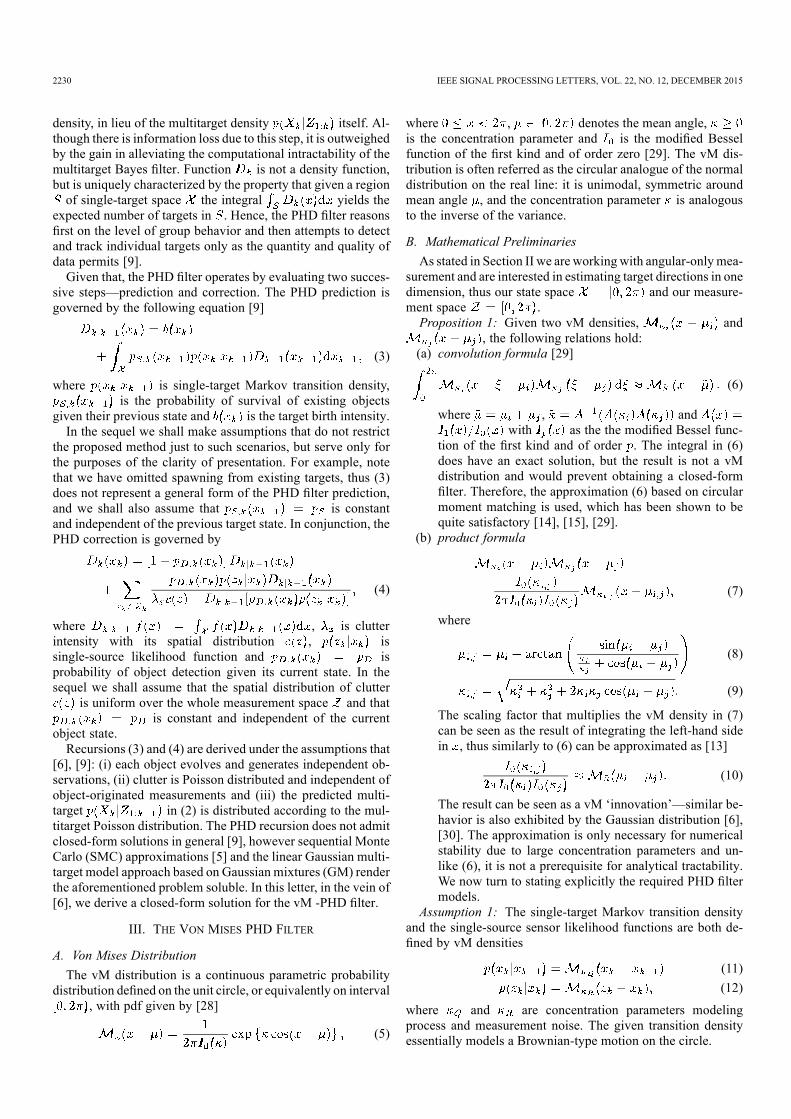
2230 IEEE SIGNAL PROCESSING LETTERS, VOL. 22, NO. 12, DECEMBER 2015
density, in lieu of the multitarget density itself. Al-though there is information loss due to this step, it is outweighedby the gain in alleviating the computational intractability of themultitarget Bayes filter. Function is not a density function,but is uniquely characterized by the property that given a regionof single-target space the integral yields the
expected number of targets in . Hence, the PHD filter reasonsfirst on the level of group behavior and then attempts to detectand track individual targets only as the quantity and quality ofdata permits [9].Given that, the PHD filter operates by evaluating two succes-
sive steps—prediction and correction. The PHD prediction isgoverned by the following equation [9]
(3)
where is single-target Markov transition density,is the probability of survival of existing objects
given their previous state and is the target birth intensity.In the sequel we shall make assumptions that do not restrict
the proposed method just to such scenarios, but serve only forthe purposes of the clarity of presentation. For example, notethat we have omitted spawning from existing targets, thus (3)does not represent a general form of the PHD filter prediction,and we shall also assume that is constantand independent of the previous target state. In conjunction, thePHD correction is governed by
(4)
where , is clutterintensity with its spatial distribution , issingle-source likelihood function and isprobability of object detection given its current state. In thesequel we shall assume that the spatial distribution of clutter
is uniform over the whole measurement space and thatis constant and independent of the current
object state.Recursions (3) and (4) are derived under the assumptions that
[6], [9]: (i) each object evolves and generates independent ob-servations, (ii) clutter is Poisson distributed and independent ofobject-originated measurements and (iii) the predicted multi-target in (2) is distributed according to the mul-titarget Poisson distribution. The PHD recursion does not admitclosed-form solutions in general [9], however sequential MonteCarlo (SMC) approximations [5] and the linear Gaussian multi-target model approach based on Gaussian mixtures (GM) renderthe aforementioned problem soluble. In this letter, in the vein of[6], we derive a closed-form solution for the vM -PHD filter.
III. THE VON MISES PHD FILTER
A. Von Mises DistributionThe vM distribution is a continuous parametric probability
distribution defined on the unit circle, or equivalently on interval, with pdf given by [28]
(5)
where , denotes the mean angle,is the concentration parameter and is the modified Besselfunction of the first kind and of order zero [29]. The vM dis-tribution is often referred as the circular analogue of the normaldistribution on the real line: it is unimodal, symmetric aroundmean angle , and the concentration parameter is analogousto the inverse of the variance.
B. Mathematical PreliminariesAs stated in Section II we are working with angular-onlymea-
surement and are interested in estimating target directions in onedimension, thus our state space and our measure-ment space .Proposition 1: Given two vM densities, and
, the following relations hold:(a) convolution formula [29]
(6)
where , andwith as the the modified Bessel func-
tion of the first kind and of order . The integral in (6)does have an exact solution, but the result is not a vMdistribution and would prevent obtaining a closed-formfilter. Therefore, the approximation (6) based on circularmoment matching is used, which has been shown to bequite satisfactory [14], [15], [29].
(b) product formula
(7)
where
(8)
(9)
The scaling factor that multiplies the vM density in (7)can be seen as the result of integrating the left-hand sidein , thus similarly to (6) can be approximated as [13]
(10)
The result can be seen as a vM ‘innovation’—similar be-havior is also exhibited by the Gaussian distribution [6],[30]. The approximation is only necessary for numericalstability due to large concentration parameters and un-like (6), it is not a prerequisite for analytical tractability.We now turn to stating explicitly the required PHD filtermodels.
Assumption 1: The single-target Markov transition densityand the single-source sensor likelihood functions are both de-fined by vM densities
(11)(12)
where and are concentration parameters modelingprocess and measurement noise. The given transition densityessentially models a Brownian-type motion on the circle.

MARKOVIĆ et al.: VON MISES MIXTURE PHD FILTER 2231
Assumption 2: The birth intensity function is a von Misesmixture of the form
(13)
The number of the newly birthed targets is governed by aPoisson distribution with the corresponding intensity .Assumption 3: The false alarm rate is governed by a Poisson
distribution with the corresponding intensity , while the spa-tial distribution of false alarms is considered to be uniform overthe whole measurement space , thus .
C. The Von Mises Mixture PHD Filter RecursionAt his point we finally have all the necessary ingredients to
derive the proposed vM -PHD filter.Proposition 2: Given the Assumptions 1–2 and that the pos-
terior intensity at time is a vM mixture
(14)
the predicted intensity is also a vM mixture
(15)where . What basically happensat the prediction stage is that the birth intensity function is addedto the posterior vM mixture, which is in the second sum-mation predicted to time .The predicted number of objects can be calculated by taking
the integral of (15) over the whole state space
(16)
Proposition 3: Given the Assumptions 1–3 and that the pre-dicted intensity at time is a vM mixture
(17)
where , the posterior intensity at timeis also a vM mixture of the following form
(18)
where is the number of measurements and
(19)
and and are given by (8) and (9) with andin lieu of and . The first summa-
tion accounts for the undetected components, while the doublesummation term accounts for the crossproduct of all the pre-dicted components and the obtained measurements.By taking the integral of (18) over the whole state space
we can calculate the posterior number of targets in the scene
(20)
At this stage, as in the case of the GM-PHD filter [6], at theend of each iteration we will have a vM mixture representingthe intensity function of the posterior multitarget distribution.What remains is (i) to extract the estimated states of the trackedtargets and (ii) to handle the geometrically growing number ofcomponents after each correction step (18) in order to keep thecomputational tractability.
D. PHD Mixture Component Reduction and State EstimationThe component reduction needs to be computationally cheap
since it will be executed after each iteration step. In [31] wehave analyzed and compared reduction algorithms for the ex-ponential family of distributions by using the vM distributionas a study example. Although there were several more accuratereduction techniques, the reduction based on West’s algorithm[32] was computationally the least intensive.For the distance measure in the present letter we use the sym-
metrized scaled Kullback-Leibler (KL) distance [33], which fortwo vM weighted components, and
, is given by
(21)
where is the ‘standard’ KL distance [34] be-tween two vM densities [31]
(22)
The West’s algorithm works on the principle of ordering themixture components according to their weights and then findsthe closest component to the first one according to the chosendistance measure. Then, the closest pair of components ismerged and the resulting one is inserted back into the mixtureper its respective weight. The merged componenthas the following parameters optimal in the KL sense
(23)
where . The procedure is repeated until thedesired, application dependent, number of components isreached. For more details regarding the reduction algorithm andcomponent merging method please confer [31].In [6] for the GM-PHD filter it was proposed to estimate the
states of the tracked targets by picking components withlargest weights. We follow the same train of though except that
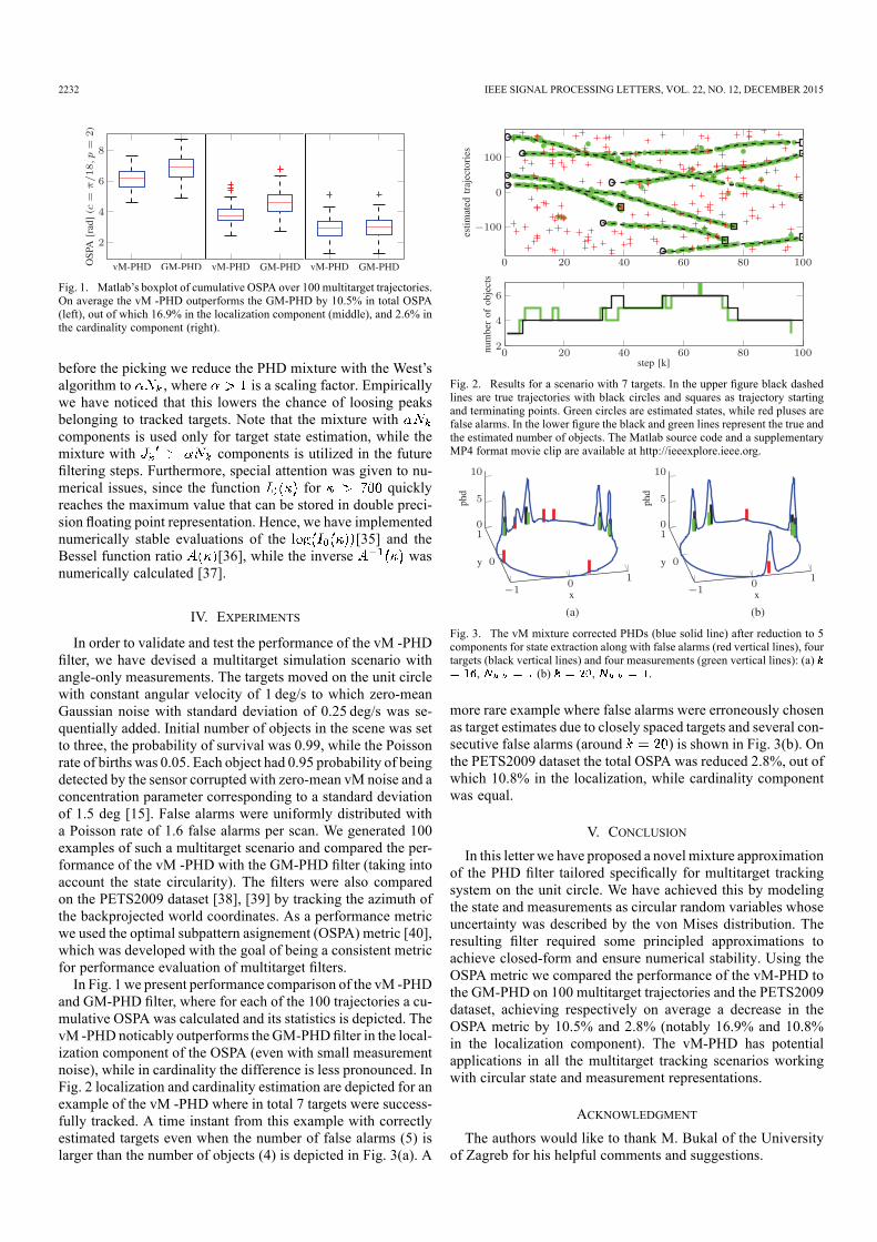
2232 IEEE SIGNAL PROCESSING LETTERS, VOL. 22, NO. 12, DECEMBER 2015
Fig. 1. Matlab’s boxplot of cumulative OSPA over 100 multitarget trajectories.On average the vM -PHD outperforms the GM-PHD by 10.5% in total OSPA(left), out of which 16.9% in the localization component (middle), and 2.6% inthe cardinality component (right).
before the picking we reduce the PHD mixture with the West’salgorithm to , where is a scaling factor. Empiricallywe have noticed that this lowers the chance of loosing peaksbelonging to tracked targets. Note that the mixture withcomponents is used only for target state estimation, while themixture with components is utilized in the futurefiltering steps. Furthermore, special attention was given to nu-merical issues, since the function for quicklyreaches the maximum value that can be stored in double preci-sion floating point representation. Hence, we have implementednumerically stable evaluations of the [35] and theBessel function ratio [36], while the inverse wasnumerically calculated [37].
IV. EXPERIMENTS
In order to validate and test the performance of the vM -PHDfilter, we have devised a multitarget simulation scenario withangle-only measurements. The targets moved on the unit circlewith constant angular velocity of 1 deg/s to which zero-meanGaussian noise with standard deviation of 0.25 deg/s was se-quentially added. Initial number of objects in the scene was setto three, the probability of survival was 0.99, while the Poissonrate of births was 0.05. Each object had 0.95 probability of beingdetected by the sensor corrupted with zero-mean vM noise and aconcentration parameter corresponding to a standard deviationof 1.5 deg [15]. False alarms were uniformly distributed witha Poisson rate of 1.6 false alarms per scan. We generated 100examples of such a multitarget scenario and compared the per-formance of the vM -PHD with the GM-PHD filter (taking intoaccount the state circularity). The filters were also comparedon the PETS2009 dataset [38], [39] by tracking the azimuth ofthe backprojected world coordinates. As a performance metricwe used the optimal subpattern asignement (OSPA) metric [40],which was developed with the goal of being a consistent metricfor performance evaluation of multitarget filters.In Fig. 1 we present performance comparison of the vM -PHD
and GM-PHD filter, where for each of the 100 trajectories a cu-mulative OSPA was calculated and its statistics is depicted. ThevM -PHDnoticably outperforms theGM-PHDfilter in the local-ization component of the OSPA (even with small measurementnoise), while in cardinality the difference is less pronounced. InFig. 2 localization and cardinality estimation are depicted for anexample of the vM -PHD where in total 7 targets were success-fully tracked. A time instant from this example with correctlyestimated targets even when the number of false alarms (5) islarger than the number of objects (4) is depicted in Fig. 3(a). A
Fig. 2. Results for a scenario with 7 targets. In the upper figure black dashedlines are true trajectories with black circles and squares as trajectory startingand terminating points. Green circles are estimated states, while red pluses arefalse alarms. In the lower figure the black and green lines represent the true andthe estimated number of objects. The Matlab source code and a supplementaryMP4 format movie clip are available at http://ieeexplore.ieee.org.
Fig. 3. The vM mixture corrected PHDs (blue solid line) after reduction to 5components for state extraction along with false alarms (red vertical lines), fourtargets (black vertical lines) and four measurements (green vertical lines): (a)
, (b) , .
more rare example where false alarms were erroneously chosenas target estimates due to closely spaced targets and several con-secutive false alarms (around ) is shown in Fig. 3(b). Onthe PETS2009 dataset the total OSPA was reduced 2.8%, out ofwhich 10.8% in the localization, while cardinality componentwas equal.
V. CONCLUSIONIn this letter we have proposed a novel mixture approximation
of the PHD filter tailored specifically for multitarget trackingsystem on the unit circle. We have achieved this by modelingthe state and measurements as circular random variables whoseuncertainty was described by the von Mises distribution. Theresulting filter required some principled approximations toachieve closed-form and ensure numerical stability. Using theOSPA metric we compared the performance of the vM-PHD tothe GM-PHD on 100 multitarget trajectories and the PETS2009dataset, achieving respectively on average a decrease in theOSPA metric by 10.5% and 2.8% (notably 16.9% and 10.8%in the localization component). The vM-PHD has potentialapplications in all the multitarget tracking scenarios workingwith circular state and measurement representations.
ACKNOWLEDGMENT
The authors would like to thank M. Bukal of the Universityof Zagreb for his helpful comments and suggestions.

MARKOVIĆ et al.: VON MISES MIXTURE PHD FILTER 2233
REFERENCES
[1] M. Mallick, B.-N. Vo, T. Kirubarajan, and S. Arulampalam, “Introduc-tion to the on multitarget tracking,” IEEE J. Sell. Topics Signal Pro-cessi., vol. 7, no. 3, pp. 373–375, Jun. 2013.
[2] D. Reid, “An algorithm for tracking multiple targets,” IEEE Trans. Au-tomat. Contr., vol. 24, no. 6, pp. 843–854, 1979.
[3] Y. Bar-Shalom and E. Tse, “Sonar tracking of multiple targets usingjoint probabilistic data association filter,” Automatica, vol. 11, pp.451–460, 1975.
[4] R. P. S. Mahler, “Multitarget Bayes filtering via first-order multitargetmoments,” IEEE Trans. Aerosp. Electron. Syst., vol. 39, no. 4, pp.1152–1178, Oct. 2003.
[5] B.-N. Vo, S. Singh, and A. Doucet, “Sequential Monte Carlo methodsfor multi-target filtering with random finite sets,” IEEE Trans. Aerosp.Electron. Syst., vol. 41, no. 4, pp. 1224–1245, Oct. 2005.
[6] B.-N. Vo and W.-K. Ma, “The Gaussian mixture probability hypoth-esis density filter,” IEEE Trans. Signal Processing, vol. 54, no. 11, pp.4091–4104, Nov. 2006.
[7] R. Mahler, “PHD filters of higher order in target number,” IEEE Trans.Aerosp. Electron. Syst., vol. 43, no. 4, pp. 1523–1543, 2007.
[8] B.-T. Vo, B.-N. Vo, and A. Cantoni, “Analytic implementations of thecardinalized probability hypothesis density filter,” IEEE Trans. SignalProcess., vol. 55, no. 7, pp. 3553–3567, Jul. 2007.
[9] R. Mahler, Statistical Multisource-Multitarget Information Fusion.Norwood, MA, USA: Arthech House, 2007.
[10] B. T. Vo, B. N. Vo, and A. Cantoni, “The cardinality balancedmulti-target multi-Bernoulli filter and its implementations,” IEEETrans. Signal Process., vol. 57, no. 2, pp. 409–423, 2009.
[11] S. Reuter, B. T. Vo, B. N. Vo, and K. Dietmayer, “The labeledmulti-Bernoulli filter,” IEEE Trans. Signal Process., vol. 62, no. 12,pp. 3246–3260, 2014.
[12] H. Deusch, S. Reuter, and K. Dietmayer, “The labeled multi-BernoulliSLAM filter,” IEEE Signal Process. Lett., vol. 22, no. 10, pp.1561–1565, 2015.
[13] I. Marković, “Moving objects detection and tracking by omnidirec-tional sensors of a mobile robot,” Ph.D. dissertation, Univ. Zagreb, Fac.Elect. Eng. Comput., , Zagreb, Croatia, 2014.
[14] M. Azmani, S. Reboul, J.-B. Choquel, and M. Benjelloun, “A recur-sive fusion filter for angular data,” in IEEE Int. Conf. Robotics andBiomimetics (ROBIO), Dec. 2009, pp. 882–887.
[15] G. Kurz, I. Gilitschenski, and U. D. Hanebeck, “Recursive monlinearfiltering for angular data based on circular distributions,” in AmericanControl Conf. (ACC), 2013, pp. 5439–5445.
[16] J. Traa and P. Smaragdis, “A wrapped Kalman filter for azimuthalspeaker tracking,” IEEE Signal Process. Lett., vol. 20, no. 12, pp.1257–1260, 2013.
[17] D. F. Crouse, “Maximum-likelihood post-detection radar ambiguityresolution,” IEEE Trans. Aerosp. Electron. Syst., vol. 50, no. 3, pp.1876–1883, 2014.
[18] Y. Yi and H. Xu, “Hierarchical data association framework with oc-clusion handling for multiple targets tracking,” IEEE Signal Process.Lett., vol. 21, no. 3, pp. 288–291, Mar. 2014.
[19] G. Kurz, I. Gilitschenski, S. Julier, and U. D. Hanebeck, “Recursivebingham filter for directional estimation involving 180 degree sym-metry,” J. Adv. Inf. Fusion, vol. 9, no. 2, pp. 90–105, 2014.
[20] V. Cevher, R. Velmurugan, and J. H. McClellan, “Acoustic multitargettracking using direction-of-arrival batches,” IEEE Trans. SignalProcess., vol. 55, no. 6, pp. 2810–2825, 2007.
[21] S. Calderara, A. Prati, and R. Cucchiara, “Mixtures of von Mises dis-tributions for people trajectory shape analysis,” IEEE Trans. CircuitsSyst. Video Technol., vol. 21, no. 4, pp. 457–471, 2011.
[22] I. Marković and I. Petrović, “Bearing-only tracking with a mixture ofvonMises distributions,” in IEEE/RSJ Int. Conf. Intelligent Robots andSystems (IROS), 2012, pp. 707–712.
[23] I. Marković, A. Portello, P. Danès, and I. Petrović, “Active speaker lo-calizationwith circular likelihoods andbootstrapfiltering,” in IEEE/RSJInt. Conf. Intelligent Robots and Systems (IROS), 2013, pp. 2914–2920.
[24] B. T. Vo and B. N. Vo, “Labeled random finite sets and multi-objectconjugate priors,” IEEE Trans. Signal Process., vol. 61, no. 13, pp.3460–3475, 2013.
[25] B. N. Vo, B. T. Vo, and D. Phung, “Labeled random finite sets and theBayes multi-target tracking filter,” IEEE Trans. Signal Process., vol.62, no. 24, pp. 6554–6567, 2014.
[26] H. G. Hoang, B.-T. Vo, and B.-N. Vo, “A generalized labeled multi-Bernoulli filter implementation using Gibbs sampling,” arXiv:1506.00821, 2015.
[27] F. Papi, B.-N. Vo, B.-T. Vo, C. Fantacci, and M. Beard, “General-ized labeled multi-Bernoulli approximation of multi-object densities,”arXiv:1412.5294, 2014.
[28] R. von Mises, “Uber die ‘Ganzzahligkeit’ der Atomgewicht und Ver-wandte Fragen,” Phys. Zeitschrift, vol. 19, pp. 490–500, 1918.
[29] K. V. Mardia and P. E. Jupp, Directional Statistics. New York, NY,USA: Wiley, 1999.
[30] H. W. Sorenson and D. L. Alspach, “Recursive Bayesian estimationusing Gaussian sums,” Automatica, vol. 7, no. 1, pp. 465–479, 1971.
[31] M. Bukal, I. Marković, and I. Petrović, “Composite distance basedapproach to von Mises mixture reduction,” Inf. Fusion, vol. 20, pp.136–145, 2014.
[32] M. West, “Approximating posterior distributions by mixtures,” J. Roy.Statist. Soc. B, vol. 55, no. 2, pp. 409–442, 1993.
[33] S. Amari, “Alpha-divergence is unique, belonging to both f-divergenceand Bregman divergence classes,” IEEE Trans. Inf. Theory, vol. 55, no.11, pp. 4925–4931, 2009.
[34] S. Kullback, Information Theory and Statistics. New YorkNew York,NY, USA: Dover, 1997.
[35] A. Tanabe, K. Fukumizu, S. Oba, T. Takenouchi, and S. Ishii, “Pa-rameter estimation for von Mises–Fisher distributions,” Computati.Statist., vol. 22, no. 1, pp. 145–157, 2007.
[36] W. Gautschi and J. Slavik, “On the computation of modified Besselfunction ratios,”Math. Computat., vol. 32, no. 143, pp. 865–875, 1978.
[37] J. P. Marques de Sá, Applied Statistics using SPSS, Statistica, Matlaband R. Berlin, Germany: Springer-Verlag, 2007.
[38] J. Ferryman and A. Shahrokni, “PETS2009: Dataset and challenge,” inIEEE Int. Workshop on Performance Evaluation of Tracking Surveil-lance, 2009.
[39] L. Leal-Taixé, A. Milan, I. Reid, S. Roth, and K. Schindler,“MOTChallenge 2015: Towards a benchmark for multi-targettracking,” arXiv:1504.01942 [cs], 2015.
[40] D. Schuhmacher, B. T. Vo, and B. N. Vo, “A consistent metric forperformance evaluation of multi-object filters,” IEEE Trans. SignalProcess., vol. 56, pp. 3447–3457, 2008.

68 publications
publication 2
I. Marković, J. Ćesić and I. Petrović. On wrapping the Kalman lter and estimating with
the SO(2) group. International Conference on Information Fusion (FUSION). Heidelberg,
Germany, 2245–2250, 2016.

On wrapping the Kalman filter and estimating withthe SO(2) group
Ivan Markovic, Josip Cesic, Ivan PetrovicUniversity of Zagreb, Faculty of Electrical Engineering and Computing, Unska 3, 10000 Zagreb, Croatia
Email: [email protected], [email protected], [email protected]
Abstract—This paper analyzes directional tracking in 2D withthe extended Kalman filter on Lie groups (LG-EKF). The studystems from the problem of tracking objects moving in 2DEuclidean space, with the observer measuring direction only,thus rendering the measurement space and object position onthe circle—a non-Euclidean geometry. The problem is furtherinconvenienced if we need to include higher-order dynamics in thestate space, like angular velocity which is a Euclidean variables.The LG-EKF offers a solution to this issue by modeling the statespace as a Lie group or combination thereof, e.g., SO(2) or itscombinations with Rn. In the present paper, we first derive theLG-EKF on SO(2) and subsequently show that this derivation,based on the mathematically grounded framework of filteringon Lie groups, yields the same result as heuristically wrappingthe angular variable within the EKF framework. This resultapplies only to the SO(2) and SO(2)× Rn LG-EKFs and is notintended to be extended to other Lie groups or combinationsthereof. In the end, we showcase the SO(2) × R2 LG-EKF, asan example of a constant angular acceleration model, on theproblem of speaker tracking with a microphone array for whichreal-world experiments are conducted and accuracy is evaluatedwith ground truth data obtained by a motion capture system.
I. INTRODUCTION
In moving object tracking, it is not uncommon to workwith sensors that can provide only direction to the object inquestion. The measurement and estimation state space havea specific geometry of their own, which is different from thegeometry of the true trajectory space. The problem is challeng-ing, because, although the motion of the object resides eitherin 3D or 2D Euclidean space, corresponding measurementsreside either on the sphere or the circle, respectively. Namely,if we are measuring and estimating only the direction to theobject in 2D, i.e., the azimuth, the state and measurements willbear the non-Euclidean properties of angles. However, if weare to extend the state space so that it includes both the angularvelocity and acceleration (which are Euclidean variables), sothat we can apply a higher-order dynamic motion model, weare faced with constructing a ‘hybrid’ state space consistingof both the non-Euclidean and Euclidean variables.
There exist Bayesian methods based on the principle ofassumed density filtering with directional distributions onthe circle, namely the von Mises distribution, the wrappedGaussian distribution and the Bingham distribution (whichactually models variables with 180 symmetry), that captureintrinsically the non-Euclidean nature of angular random vari-ables [1]–[6]. The benefit of these approaches is that theytake globally into account the geometry of the state space.
For example, in the case of the von Mises distribution it hasbeen shown that the filter outperforms the naive Kalman filter,which treats angles like regular Euclidean variables, and themodified Kalman filter, which takes into account the natureof angles by wrapping them on the circle [4], [7]. However,extending the state space with additional variables of differentgeometry, e.g., to analytically model the azimuth with thevon Mises distribution and the range or the angular velocitywith the Gaussian distribution and capture correctly the cross-correlations, remains a challenge.
The SO(2) group is a set of orthogonal matrices with deter-minant one, whose elements geometrically represent rotations.This makes it an interesting candidate for estimation withangular variables. Furthermore, a filter could be derived notjust for SO(2), but also for combinations of SO(2) with R.This would enable us to create the aforementioned ‘hybrid’state vector that would join both non-Euclidean and Euclideanvariables within the same filter and enable a seamless uti-lization of higher-order system models with constant angularvelocity or acceleration. An extended Kalman filter on matrixLie groups was recently proposed in [8]. It provides us with amathematical framework for solving the ‘hybrid’ state spaceproblem. Indeed, the filter can be applied directly for anystate that is a combination of Lie groups, since a Cartesianproduct of Lie groups is a Lie group [8]. However, it shouldbe noted that the LG-EKF is a local approach, in the sense thatit does not take globally the geometry of the state space intoaccount, but locally captures the geometry of state space viaexponential mapping. Another approach would be to model thewhole state space as a Euclidean vector within the ‘classical’Kalman filter framework, and wrap the operations involvingangular variables. Indeed, this was performed in [4] to modifythe unscented Kalman filter for angular state estimation, in [9]to take idiosyncrasies of directional statistics when using polaror spherical coordinates in the cubature Kalman filter, and in[7] to modify the Gaussian mixture probabilistic hypothesisdensity filter for multitarget tracking on a circle.
In this paper we propose to analyze the LG-EKF fordirectional tracking of moving objects in 2D. First, we lookinto deriving the LG-EKF on the SO(2), which also servesas a gentle introduction to the subject matter since the LG-EKF introduces non-trivial notation. Second, we model thedirectional moving object tracking in 2D as an estimationproblem on the Lie group composed of the direct productSO(2) × R2, i.e., a group that represents the moving object
19th International Conference on Information Fusion Heidelberg, Germany - July 5-8, 2016
978-0-9964527-4-8©2016 ISIF

azimuth, angular velocity and angular acceleration. For themotion model, we use the constant angular acceleration model.In the end, we show that the SO(2) LG-EKF filter derivationbased on the mathematically grounded framework of filteringon Lie groups yields the same result as heuristically wrappingthe angular variables within the extended Kalman filter (EKF)framework. Since for the case of Rn the LG-EKF evaluatesto EKF [8], this results also extends to SO(2) × R2 LG-EKF and an R3 EKF when wrapping the angular component.Please note that this result applies only to the SO(2) filterand is not intended to be extended to other Lie groups orcombinations thereof. Indeed, given that SO(2) is abelian,i.e., commutative, the result does not seem unexpected, butwe assert that it gives interesting theoretical perspective onestimation and tracking with the heuristically modified EKF.Before we proceed with the filter derivation, we introducesome necessary formal definitions and operators for workingwith matrix Lie groups.
II. MATHEMATICAL BACKGROUND
A. Wrapping the Kalman filter
In this section we shall assume that wrapping operationamounts to enforcing the angular variable to be in the [−π, π]interval, and we designate this operation as follows
wπ(x) = mod(x+ π, 2π)− π. (1)
Note that when computing the difference between two angularvariables, the wrapping effect of the circle should be taken intoaccount, e.g., the difference between 178 and −178 shouldevaluate to 4. This is also achieved by (1) when the differenceis given as the argument, i.e., difference between two anglesx and y is computed as wπ(x− y).
Let us assume the following system model
xk+1|k = fk(xk, uk) + nk, nk ∼ N (0, Q) (2)
where xk is the system state, uk is the control input, nkis process noise, and fk( · ) is the non-linear system stateequation. In the EKF the idiosyncrasies of angular data appearmost prominently in the correction step when calculating theinnovation, which should be computed as
xk+1 = xk+1|k +Kk wπ(zk − hk(xk+1|k)), (3)
where Kk is the Kalman gain, zk is the measurement, andhk( · ) is the non-linear measurement equation.
To demonstrate this, let us take a simple example ofhaving an identity measurement equation, xk+1|k = 358,zk = 2 and Kk = 0.5. If we would not wrap the innovation,the updated state would yield a clearly incorrect result ofxk+1 = 180 inlieu of xk+1 = 360. For practical purposes,after correction and prediction the system state can be checkedto the required interval by computing xk+1 ← wπ(xk+1). Inthe sequel when we refer to the modified Kalman filter, itentails treating angular variables with the previously intro-duced operation. Furthermore, we assume that the reader isfamiliar with EKF equations, which we will not present orderive explicitly in order to keep the brevity of the paper.
B. Lie GroupsA Lie group G is a group which is also a smooth manifold
and the group composition and inverse are smooth functionson the manifold G. A manifold is an object that looks locallylike a piece of Rn and G is ‘smooth’ in the sense that ishas a tangent space, of the appropriate dimension, at eachpoint. Take for example the circle, a curve in R2 which lookslocally (but not globally) like R1. For a matrix Lie group thecomposition and inverse are simply matrix multiplication andinversion, with the identity element In×n [10].
A Lie Algebra g is an open neighborhood of 0n×n inthe tangent space of G at the identity In×n. The matrixexponential expG and matrix logarithm logG establish a localdiffeomorphism between Lie groups and Lie algebras [8]
expG : g→ G, logG : G→ g. (4)
The Lie Algebra g associated to a p-dimensional matrix Liegroup G ⊂ Rn×n is a p-dimensional vector space [10]. Alinear isomorphism between g and Rp is given by
[·]∨G : g→ Rp, [·]∧G : Rp → g. (5)
Lie Groups are not necessarily commutative. The followingtwo operators capture this property• the adjoint representation of G on Rp
AdG : AdG(X)x =[X[x]∧GX
−1]∨G (6)
• the adjoint representation of Rp on Rp
adG : adG(x)y = [[x]∧G [y]∧G − [y]∧G [x]∧G ]∨G (7)
where x, y ∈ Rp. In the sequel, these operators, the exponen-tial and logarithmic mapping are given concrete form for thepertinent Lie groups.
C. The SO(2) groupIn this example our system state (azimuth of the tracked
object) is modeled as the group G = SO(2), i.e., as the rotationmatrix Xk = Rθk
Rθk =
[cos θk − sin θksin θk cos θk
]. (8)
The composition and inverse in SO(2) are simply evaluatedas X1X2 = R1R2, X
−1 = RT. For this case the associatedLie algebra which bridges Xk ∈ G and xk = θk ∈ R1 isg = so(2), and the following holds
[θk]∧G =
[0 −θkθk 0
]. (9)
The link between SO(2) and so(2) is given by the exponentialand logarithmic mapping
expG([θk]∧G) = Rθk : so(2)→ SO(2), (10)logG(Rθk) = [θk]∧G : SO(2)→ so(2). (11)
Due to the commutativity of SO(2), the adjoint operators are
adG(θk) = 0, AdG (expG ([θk]∧G)) = 1. (12)
These properties greatly simplify the LG-EKG formulae forthe SO(2) group which will become evident in the sequel.

D. The SO(2)× R2 group
In this section we propose to model the system state as theCartesian product of groups G = SO(2)×R2. This is a slightabuse of notation intended for clarity, since when talking aboutR within the group or algebra, we are actually referring to thegroup of algebra representation of R, for which the explicitrepresentation is given further in the paper. The moving objectstate Xk will represent the azimuth of the target as a rotationmatrix Rθk ∈ SO(2), angular velocity as a real number ωk ∈R, and angular acceleration also as a real number αk ∈ R.The system state Xk can be symbolically represented as
Xk =
Rk [1 ωk0 1
]
[1 αk0 1
]
=
Rkωkαk
G
. (13)
Note that composition and inverse on such a group is evaluatedas follows
X1X2 =
R1R2
ω1 + ω2
α1 + α2
G
, X−1 =
RT
−ω−α
G
. (14)
The associated Lie algebra is g = so(2)×R2 which bridgesthe state on the Lie group Xk ∈ G with the vector xk =[θk ωk αk]T ∈ R3, and the following holds
[xk]∧G =
[θk]∧SO(2)
[ωk]∧R[αk]∧R
=
[θk]∧SO(2)
ωkαk
g
,
(15)
where [θk]∧SO(2) is given by (9), while
[ωk]∧R =
[0 ωk0 0
]and [αk]∧R =
[0 αk0 0
]. (16)
The link between the group G and the associated algebra g isdefined by the exponential mapping
expG ([xk]∧G) =
expSO(2)
([θk]∧SO(2)
)
ωkαk
G
=
Rkωkαk
G
,
(17)
and logarithmic mapping
logG (Xk) =
logSO(2) (Rk)
ωkαk
g
=
[θk]∧SO(2)
ωkαk
g
. (18)
Furthermore, since SO(2) and R are abelian and the Cartesianproduct of abelian groups is abelian, the adjoint operators areagain trivial
adG(xk) = 03×3, AdG (expG ([xk]∧G)) = I3×3. (19)
III. THE EKF ON MATRIX LIE GROUPS
As in the case of classical Kalman filtering, we need tobegin by defining a motion model by which we will calculatethe prediction. For general filtering on matrix Lie groups, thesystem model is defined by the following equation [8]
Xk+1 = f(Xk, uk, nk) = Xk expG
([Ωk + nk]∧G
), (20)
where Xk ∈ G is the system state at time k, G is ap-dimensional Lie Group, nk ∼ NRp(0p×1, Qk) is whiteGaussian noise and Ωk = Ω(Xk, uk) : G × Rw → Rp isthe system state equation which describes how the modelacts on the state and control input in order to calculate thedisplacement.
Note that the function of Ωk is to take the system statewhich resides on G and the control input which resides on Rw,calculate the displacement by applying the system model, andthen transfer the displacement to the vector space Rp whereadditive noise is added. This displacement is then transferredto the associated Lie algebra by the [ . ]∧G operator and thenexponentially mapped back to the Lie group to be added byway of composition to the system state Xk. Given that, aquestion arises how to implement a specific system model,since in LG-EKF it operates through a displacement? That is,how to construct Ωk from fk(xk, uk)? The first step would beto write the system equation as fk(xk, uk) = xk + fk(xk, uk)which can then be practically ‘translated’ to appropriate Ωk.Note that generality is not lost here since −xk can be includedwithin fk(xk, uk),
The prediction step of the LG-EKF is governed by thefollowing formulae [8]
µk+1|k = µk expG
([Ωk]∧G
)(21)
Pk+1|k = FkPkFTk + ΦG(Ωk)QkΦG(Ωk)T , (22)
where µk ∈ G is the estimated mean value of the system stateXk, Pk ∈ Rp×p is the estimated covariance matrix, while otherterms are non-trivially calculated matrices
Fk = AdG
(expG
([−Ωk]∧G
))+ ΦG(Ωk)Ck, (23)
ΦG(ν) =
∞∑
m=0
(−1)m
(m+ 1)!adG(ν)m, ν ∈ Rp, (24)
Ck =∂
∂εΩ (µk expG ([ε]∧G) , uk−1)|ε=0 . (25)
The parameter ε ∈ Rp can be seen as a Lie algebraic errorwhich is approximated as being distributed according to aclassical Euclidean Gaussian distribution ε ∼ NRp(0p×1, Pk).It is interesting to note that the mean value µk resides onthe Lie group G, while the covariance matrix Pk describesuncertainty in Rp. Although at first this appears peculiar, itis a consequence of modeling the uncertainty of states onLie groups by the assumption of the concentrated Gaussiandistribution Xk ∼ G(µk, Pk). In essence, the state resides onthe group, but its uncertainty resides on the tangential vectorspace. For a more formal introduction of this concept, pleaseconfer [8].

The discrete measurement model on the matrix Lie Groupis given as follows
zk+1 = h(Xk+1) expG′ ([mk+1]∧G′) , (26)
where zk+1 ∈ G′, h : G → G′, and mk+1 ∼ NRq (0q×1, Rk)is white Gaussian noise. Note that here a different group G′ isused since the system state and measurements might belong todifferent groups. Having the measurement model defined, wecan proceed now to the update step which will first constitutethe calculation of the Kalman gain
Kk+1 = Pk+1|kHTk+1
(Hk+1Pk+1|kHTk+1 +Rk+1
)−1,(27)
where the measurement matrix Hk+1 is calculated via
Hk+1 =∂
∂ε
[logG′
(h(µk+1|k)−1
h(µk+1|k expG ([ε]∧G)
))]∨G |ε=0
.(28)
Furthermore, the innovation vector multiplied by Kalman gainis computed as
νk+1 = Kk+1
[logG′
(h(µk+1|k)−1zk+1
)]∨G′ . (29)
Finally, the update of the system state and covariance matrixcan be evaluated as [8]
µk+1 = µk+1|k expG ([νk+1]∧G) (30)
Pk+1 = ΦG(νk+1)(Ip×p −Kk+1Hk+1
)Pk+1|kΦG(νk+1)T .
(31)
We can notice similarities between the LG-EKF and EKFequations and, indeed, when G and G′ are Euclidean spaces theLG-EKF reduces to EKF [8]. Furthermore, due to the results(12) and (19), matrices Fk and ΦG(ν) for both SO(2) andSO(2)× R2 evaluate to
ΦG(ν) = I, Fk = I + Ck. (32)
In the sequel we derive the LG-EKF for the groups whichwe propose to utilize for tracking of moving objects withangular measurements and show that in this special case theLG-EKF reduces to the heuristically modified EKF.
A. LG-EKF on SO(2)
In this section we derive the LG-EKF filter for state esti-mation on G = SO(2). For this group, mathematically denseLG-EKF equations are simplified and serve well to intuitivelygrasp the mechanics of the filter.
1) Prediction: Let us take two examples of system models.In the first we assume a stationary process, i.e., in theprediction the mean value will remain unchanged except forthe uncertainty that is added through the process noise (this issimilar to the von Mises filter [1])
xk+1|k = xk + nk, nk ∼ NR1(0, σ2Q). (33)
This yields the LG-EKF system model Ω(Xk) = 0 with thesame process noise nk, which when inserted in (21) will
evaluate through the exponential as an identity matrix, thusleaving the mean value unperturbed.
In order to compute the prediction of the covariance matrixvia (22), given the result in (32), we only need to determineCk. In this case the Lie algebraic error is ε ∈ R1 and due tothe system model the matrix Ck evaluates to zero, thus leavingFk = 1, and the prediction equations are
µk+1|k = µk, Pk+1|k = Pk +Qk. (34)
As we can see, these are the same formulae that an EKFprediction would yield with (33) as the system model.
As the second example, we take the non-linear system [4]where the robot rotary joint angle was estimated
xk+1|k = xk + c1 sin(xk) + c2 + nk, (35)
where second and third term account for gravity and velocity,while the final term is again one-dimensional white Gaussiannoise. This yields the following LG-EKF system model
Ω(Xk) = c1 sin([log(Xk)]∨G) + c2. (36)
Note that [log(Xk)]∨G is necessary to bring the rotation matrixwith parameter µk to a scalar angle in R1. The Lie algebraicerror is again ε ∈ R1 and given the system model (36) matrixCk evaluates to
Ck =∂
∂εΩ
([cosµk − sinµksinµk cosµk
] [cos ε − sin εsin ε cos ε
])
|ε=0
=∂
∂εΩ
([cos(µk + ε) − sin(µk + ε)sin(µk + ε) cos(µk + ε)
])
|ε=0
=∂
∂ε(c1 sin(µk + ε) + c2)|ε=0 = c1 cosµk (37)
This means that Fk = 1 + c1 cosµk, and that the LG-EKFprediction equations are
µk+1|k = µk expG ([c1 sin([log(Xk)]∨G) + c2]∧G)
Pk+1|k = Pk(1 + c1 cosµk)2 +Qk. (38)
We can see that the covariance prediction formula is identicalto the EKF covariance prediction.
More generally, to demonstrate the equivalence of themodified EKF and SO(2) LG-EKF prediction steps we needto show that Fk = 1 + Ck is equal to
Fk =∂fk(xk, uk)
∂xk |xk=µk
, (39)
where Fk is the state transition matrix, i.e., the EKF systemstate Jacobian of (2). By inspecting (37) we can notice thatfor SO(2) the argument within Ω will always be the sum ofthe mean value and the Lie algebraic error µk + ε. This gives
Fk = 1 +∂
∂εΩ(expG([µk + ε]∧G), uk)|ε=0
= 1 +∂
∂εfk(µk + ε, uk)|ε=0
= 1 +∂
∂ε(fk(µk + ε, uk)− (µk + εθ))|ε=0
=∂fk(µk + ε, uk)
∂ε |ε=0=∂fk(ξk, uk)
∂ξk |ξk=µk
, (40)

where variable substitution was performed in the last step:ξk ← µk + ε, ∂ξk ← ∂ε. In the end Fk evaluates to the EKFJacobian Fk when the underlying group is SO(2).
2) Correction: Since we are measuring angles, we definethe measurement Lie group as G′ = SO(2) and the measure-ment function h : SO(2)→ SO(2)
h(Xk+1) = Rk+1, mk+1 ∼ NR1(0, σ2R), (41)
which is trivial since the measurement and state group are thesame, while the measurement noise is a one-dimensional whiteGaussian noise. As in the prediction step, the associated Liealgebra is g′ = so(2).
To compute the correction step, we need to evaluate (28)for the LG-EKF on SO(2). The composition of the predictedmean µk+1|k and the Lie algebraic error yields
h(µk+1|k expSO(2)([ε]∧SO(2))) =
[cos(µk+1|k + ε) − sin(µk+1|k + ε)sin(µk+1|k + ε) cos(µk+1|k + ε)
].
(42)
Since h(µk+1|k)−1 is the transpose of the correspondingrotation matrix, by inserting these results in (28) we cancalculate the measurement matrix
Hk+1 =∂
∂ε
([logG
([cos ε − sin εsin ε cos ε
])]∨
G
)
|ε=0
= 1 (43)
Given this results it is straightforward to see that Kalmangain and covariance update equation of SO(2) LG-EKF areequal to the EKF equations. The state correction equationsyield the same result, except that the LG-EKF takes wrappinginto account by composition of rotation matrices, while themodified EKF computes everything in R1 and would need towrap the corrected state with wπ( · ).
B. LG-EKF on SO(2)× R2
In this section we derive the LG-EKF filter for state estimationon G = SO(2) × R2. Given the demonstrated equality ofthe SO(2) LG-EKF and the modified EKF and that LG-EKFreduces to EKF for Euclidean spaces, it is intuitive to expectthat this result would extend to groups derived by composingSO(2) with Euclidean spaces. In the sequel we illustrate thisproperty by deriving a constant angular acceleration model fortracking with angle-only measurements.
1) Prediction: Given the state representation, we can nowdefine the system model. For this purpose, we use the constantangular acceleration model Ωk = Ω(Xk) : G→ R3
Ω(Xk) =
Tωk + 1
2T2αk
Tαk0
, nk ∼ NR3(0, Q). (44)
Note that the displacement due to motion is calculated firstin R3 and then according to (21) transferred to Lie algebrag, exponentially mapped to the group G and then by way ofcomposition added to the system state Xk.
In this case, the Lie algebraic error is ε = [εθ εω εα]T ∈ R3,hence the composition of the mean value µk and ε yields
µk expG([ε]∧G) =
RkRεωk + εωαk + εα
G
, (45)
with RkRε has the same for as the matrix product in (42). Byapplying the motion model (44) on this results we get
Ω(µk expG([ε]∧G)) =
T (ω + εω) + 1
2T2(α+ εα)
T (α+ εα)0
. (46)
To compute the prediction step for the covariance matrix, weneed to calculate matrix Fk. Since adjoint operators are trivial,using (46) we calculate
Fk = I + Ck =
1 T 12T
2
0 1 T0 0 1
. (47)
We can see that the matrix Fk evaluates to the well knowntransition matrix of the classical EKF constant accelerationmotion model.
2) Correction: Since here we track moving objects bymeasuring angles, we define the measurement Lie group G′ =SO(2) and the measurement function h : SO(2)×R2 → SO(2)
h(Xk+1) = Rk+1, mk+1 ∼ NR1(0, σ2R) (48)
which in this case simply extracts the rotation matrix Rk+1
from Xk+1. Calculation of the matrix Hk+1 is the same as in(28), except that ε is now a vector
Hk+1 =∂
∂ε(εθ)|ε=0 = [1 0 0]. (49)
Again, the same result as we would expect for the EKFmeasurement matrix.
IV. EXPERIMENTS
As a practical example of an application of the studied filterwe apply this on the problem of speaker tracking with a micro-phone array and in the present paper we test the SO(2)×R2
LG-EKF on real-world data. For the sound acquisition weused the ManyEars framework consisting of an 8-channelUSB sound card [11], while for obtaining measurements weused the beamforming algorithm for speaker localization [12]implemented under the Robot Operating Systems [13] withinthe same framework. The maximum of the beamformingenergy was picked as the speaker measurement.
The experiments were conducted in a 120 m2 room withparquet wooden flooring and one side covered with windows.The speaker was simulated by a loudspeaker playing anexcerpt from Nature’s podcast Audiophile in English. The areain which the loudspeaker moved was covered by a motioncapture system, which was used to generate ground truth data.In order to handle outliers, we used validation gating; namely,the innovation matrix Sk+1 = Hk+1Pk+1|kHT
k+1 +Rk+1 wascalculated and we applied the standard χ2–test
νk+1S−1k+1ν
Tk+1 < γ, (50)

0 20 40 60 80 100 120−200
−100
0
100
200
time [s]
θ[°
]
θRMSE = 2.24
(a) azimuth
0 20 40 60 80 100 120−20
−10
0
10
20
time [s]
ω[°
/s]
ωRMSE = 3.38 °/s
(b) angular velocity
Fig. 1: Performance of the LG-EKF on SO(2)×R2 when tracking a movingspeaker. The solid black line is the ground truth as given by the motion capturesystem, the green solid line is the estimated state of the speaker, while thegray circles represent measurements, i.e. outputs of the beamformer. StateRMSE is given in the title of each of the subfigures.
where the threshold γ was determined from the inverse χ2p
cumulative distribution at a significance level a = 0.95 andp degrees-of-freedom. Figure 1 shows the experiment resultsand corroborates that the filter successfully manages to trackthe moving speaker in spite of the number of outliers. Notethat the modified EKF would yield the same results, exceptthat in the case of the LG-EKF the system state was definedon SO(2) × R2 and the idiosyncrasies of angular data wereintrinsically taken care of.
V. CONCLUSION
In this paper we have studied directional moving objecttracking in 2D based on the extended Kalman filter on matrixLie groups. First, we have proposed to analyze this estimation
problem by modeling the state to reside on the SO(2) group.Subsequently, we have shown that the SO(2) filter derivationbased on the mathematically grounded framework of filteringon Lie groups yields evaluates to heuristically wrapping theextended Kalman filter. We emphasize that this result appliesonly to the SO(2) filter and is not intended to be extendedto other Lie groups or combinations thereof. Second, we havederived the constant angular velocity SO(2)×R2 filter, wherethe system state consisted of azimuth, angular velocity andangular acceleration. For this filter we showcased a real-worldexperiment of a speaker tracking problem with a microphonearray by assessing the accuracy using the ground truth obtainedby a motion capture system.
ACKNOWLEDGMENTS
This work has been supported from the European Union’sHorizon 2020 research and innovation programme under grantagreement No 688117 (SafeLog) and the Unity ThroughKnowledge Fund under the project Cooperative Cloud basedSimultaneous Localization and Mapping in Dynamic Environ-ments.
REFERENCES
[1] M. Azmani, S. Reboul, J.-B. Choquel, and M. Benjelloun, “A recursivefusion filter for angular data,” in IEEE International Conference onRobotics and Biomimetics (ROBIO), dec 2009, pp. 882–887.
[2] I. Markovic and I. Petrovic, “Speaker localization and tracking with amicrophone array on a mobile robot using von Mises distribution andparticle filtering,” Robotics and Autonomous Systems, vol. 58, no. 11,pp. 1185–1196, 2010.
[3] ——, “Bearing-only tracking with a mixture of von Mises distributions,”in IEEE/RSJ International Conference on Intelligent Robots and Systems(IROS), 2012, pp. 707–712.
[4] G. Kurz, I. Gilitschenski, and U. D. Hanebeck, “Recursive monlinearfiltering for angular data based on circular distributions,” in AmericanControl Conference (ACC), 2013, pp. 5439–5445.
[5] G. Kurz, I. Gilitschenski, S. Julier, and U. D. Hanebeck, “Recursiveestimation of orientation based on the Bingham distribution,” in Inter-national Conference on Information Fusion (FUSION), 2013, pp. 1–16.
[6] G. Stienne, S. Reboul, M. Azmani, J. Choquel, and M. Benjelloun, “Amulti-temporal multi-sensor circular fusion filter,” Information Fusion,vol. 18, pp. 86–100, jul 2014.
[7] I. Markovic, J. Cesic, and I. Petrovic, “Von Mises mixture PHD filter,”IEEE Signal Processing Letters, vol. 22, no. 12, pp. 2229–2233, 2015.
[8] G. Bourmaud, R. Megret, M. Arnaudon, and A. Giremus, “Continuous-discrete extended Kalman filter on matrix Lie groups using concentratedGaussian distributions,” Journal of Mathematical Imaging and Vision,vol. 51, no. 1, pp. 209–228, 2015.
[9] D. F. Crouse, “Cubature / Unscented / Sigma Point Kalman Filteringwith Angular Measurement Models,” in International Conference onInformation Fusion, 2015, pp. 1550–1557.
[10] G. S. Chirikjian, Stochastic Models, Information Theory, and LieGroups, Volume 2: Analytic Methods and Modern Applications.Springer, 2012.
[11] F. Grondin, D. Letourneau, F. Ferland, V. Rousseau, and F. Michaud,“The ManyEars open framework,” Autonomous Robots, vol. 34, no. 3,pp. 217–232, 2013.
[12] J.-M. Valin, F. Michaud, and J. Rouat, “Robust localization and trackingof simultaneous moving sound sources using beamforming and particlefiltering,” Robotics and Autonomous Systems, vol. 55, no. 3, pp. 216–228, 2007.
[13] M. Quigley, B. Gerkey, K. Conley, J. Faust, T. Foote, J. Leibs, E. Berger,R. Wheeler, and A. Ng, “ROS : an open-source Robot OperatingSystem,” IEEE International Conference on Robotics and Automation(ICRA), Workshop on Open Source Software, 2009.

publications 75
publication 3
J. Ćesić, I. Marković and I. Petrović. Moving object tracking employing rigid body motion
onmatrix Lie groups. International Conference on Information Fusion (FUSION). Heidelberg,
Germany, 2109–2115, 2016.

Moving object tracking employing rigid bodymotion on matrix Lie groups
Josip Cesic, Ivan Markovic, Ivan PetrovicUniversity of Zagreb, Faculty of Electrical Engineering and Computing, Unska 3, 10000 Zagreb, Croatia
Email: [email protected], [email protected], [email protected]
Abstract—In this paper we propose a novel method forestimating rigid body motion by modeling the object state directlyin the space of the rigid body motion group SE(2). It hasbeen recently observed that a noisy manoeuvring object inSE(2) exhibits banana-shaped probability density contours inits pose. For this reason, we propose and investigate two statespace models for moving object tracking: (i) a direct productSE(2) × R3 and (ii) a direct product of the two rigid bodymotion groups SE(2) × SE(2). The first term within these twostate space constructions describes the current pose of the rigidbody, while the second one employs its second order dynamics,i.e., the velocities. By this, we gain the flexibility of trackingomnidirectional motion in the vein of a constant velocity model,but also accounting for the dynamics in the rotation component.Since the SE(2) group is a matrix Lie group, we solve thisproblem by using the extended Kalman filter on matrix Liegroups and provide a detailed derivation of the proposed filters.We analyze the performance of the filters on a large number ofsynthetic trajectories and compare them with (i) the extendedKalman filter based constant velocity and turn rate model and(ii) the linear Kalman filter based constant velocity model. Theresults show that the proposed filters outperform the other twofilters on a wide spectrum of types of motion.
I. INTRODUCTION
A wide area of robotics research has extensively focused onthe practical approaches of using different types of manifolds.Besides performance, filters operating on manifolds canprovide other advantages as they avoid singularities whenrepresenting state spaces with either redundant degrees offreedom or constraint issues [1], [2]. Among the manifolds,the homogeneous transformation matrices, also referred to asthe rigid body motion group SE(n), hold a special repute.They have been used in a variety of applications, and haverisen to popularity firstly through manipulator robotics [3], [4]and later through vision applications [5], [6]. Even though thestate description using the rigid body motion group, for boththe 2D and 3D case, has been a well known representation,techniques for associating the uncertainty came into focuslater [7]. So far, the rigid body motion group with associateduncertainty has been used in several robotics applicationssuch as SLAM [8], motion control [9], shape estimation [10],pose estimation [11] and pose registration [12].
Among them, pose estimation represents one of the centralproblems in robotics. Recently in [11] the authors discussedthe advantages of employing uncertainties on SE(2) (thereincalled the exponential coordinates) with respect to Euclideanspaces and have provided the means for working in theexponential coordinates rather than representing the robot’s
Fig. 1: An illustration of an omnidirectional mobile robotmanoeuvring in both translational and rotational components. Thebanana shaped uncertainty contours, representing the positionaluncertainty in the next step, are formed by modeling the uncertaintyon the SE(2) group (blue), while the elliptical shaped contours appearmodeling the uncertainty in R2 (gray).
position with Gaussians in Cartesian coordinates. This stemsfrom the fact that the uncertain robot motion, and consequentlyits pose, usually exhibit banana-shaped probability densitycontours rather than the elliptical ones [13], as illustrated inFig. 1. The classical Kalman filter is designed to operatein the Cartesian space and as such does not provide aframework for filtering directly on the SE(2) group. Recently,some works have addressed the uncertainty on the SE(2)group proposing new distributions [14], [15]. However, theseinteresting approaches do not yet provide a closed-formBayesian recursion framework (involving both the predictionand update) that can include higher order motion and non-linear models.
An extended Kalman filter on matrix Lie groups (LG-EKF)has been recently proposed in [16]. It provides an estimationframework for filtering directly on matrix Lie groups, of whichthe SE(2) group is a member. In accordance with the needs ofmoving object state estimation problems, higher order motionoften needs to be exploited, as in the vein of the constantvelocity (CV) or acceleration motion models [17], but in thespace such as the rigid body motion group SE(2). In thepresent paper we propose a method for moving object trackingemploying its second order motion directly on the SE(2) groupbased on the discrete LG-EKF. For this purpose, we model thestate space either as a direct product of (i) a rigid body motiongroup and a Euclidean vector or (ii) two rigid body motiongroups, i.e.,
(i) SE(2)× R3 or (ii) SE(2)× SE(2) = SE(2)2. (1)
In both cases the first term tracks the pose of the object, while
19th International Conference on Information Fusion Heidelberg, Germany - July 5-8, 2016
978-0-9964527-4-8©2016 ISIF
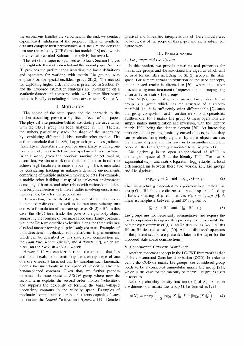
the second one handles the velocities. In the end, we conductexperimental validation of the proposed filters on syntheticdata and compare their performance with the CV and constantturn rate and velocity (CTRV) motion models [18] used withinthe classical extended Kalman filter (EKF) framework.
The rest of the paper is organized as follows. Section II givesan insight into the motivation behind the present paper. SectionIII provides the preliminaries including the basic definitionsand operators for working with matrix Lie groups, withemphasis on the special euclidean group SE(2). The methodfor exploiting higher order motion is presented in Section IVand the proposed estimation strategies are investigated on asynthetic dataset and compared with two Kalman filter basedmethods. Finally, concluding remarks are drawn in Section V.
II. MOTIVATION
The choice of the state space and the approach to themotion modelling present a significant focus of this paper.The physical interpretation behind associating the uncertaintywith the SE(2) group has been analyzed in [11]. Therein,the authors particularly study the shape of the uncertaintyby considering differential drive mobile robot motion. Theauthors conclude that the SE(2) approach provides significantflexibility in describing the position uncertainty, enabling oneto analytically work with banana-shaped uncertainty contours.In this work, given the previous moving object trackingdiscussion, we aim to track omnidirectional motion in order toachieve high flexibility in motion modeling. This is motivatedby considering tracking in unknown dynamic environmentscomprising of multiple unknown moving objects. For example,a mobile robot building a map of an unknown environmentconsisting of humans and other robots with various kinematics,or a busy intersection with mixed traffic involving cars, trams,motorcycles, bicycles and pedestrians.
By searching for the flexibility to control the velocities inboth x and y direction, as well as the rotational velocity, onecomes to formulation of the state space as SE(2)×R3. In thiscase, the SE(2) term tracks the pose of a rigid body objectsupporting the forming of banana-shaped uncertainty contours,while the R3 term describes velocities along the three axis in aclassical manner forming elliptical-only contours. Examples ofomnidirectional mechanical robot platforms implementationswhich can be described by this state space construction arethe Palm Pilot Robot, Uranus, and Killough [19], which arebased on the Swedish 45/90 wheels.
However, if we consider a robot construction that hasadditional flexibility of controling the steering angle of oneor more wheels, it turns out that by sampling such kinematicmodels the uncertainty in the space of velocities also hasbanana-shaped contours. Given that, we further proposeto model the state space as SE(2)2 group where now thesecond term exploits the second order motion (velocities),and supports the flexibility of forming the banana-shapeduncertainty contours in the velocity space. Examples ofmechanical omnidirectional robot platforms capable of suchmotion are the Nomad XR4000 and Hyperion [19]. Detailed
physical and kinematic interpretations of these models are,however, out of the scope of this paper and are a subject forfuture work.
III. PRELIMINARIES
A. Lie groups and Lie algebra
In this section, we provide notations and properties formatrix Lie groups and the associated Lie algebras which willbe used for the filter including the SE(2) group in the statespace. For a more formal introduction of the used concepts,the interested reader is directed to [20], where the authorprovides a rigorous treatment of representing and propagatinguncertainty on matrix Lie groups.
The SE(2), specifically, is a matrix Lie group. A Liegroup is a group which has the structure of a smoothmanifold, i.e., it is sufficiently often differentiable [2], suchthat group composition and inversion are smooth operations.Furthermore, for a matrix Lie group G these operations aresimply matrix multiplication and inversion, with the identitymatrix In×n being the identity element [20]. An interestingproperty of Lie groups, basically curved objects, is that theycan be almost completely captured by a flat object, such asthe tangential space; and this leads us to an another importantconcept—the Lie algebra g associated to a Lie group G.
Lie algebra g is an open neighborhood of 0n×n inthe tangent space of G at the identity In×n. The matrixexponential expG and matrix logarithm logG establish a localdiffeomorphism between these two worlds, i.e., Lie groupsand Lie algebras
expG : g→ G and logG : G→ g. (2)
The Lie algebra g associated to a p-dimensional matrix Liegroup G ⊂ Rn×n is a p-dimensional vector space defined bya basis consisting of p real matrices Ei, i = 1, .., p [9]. Alinear isomorphism between g and Rp is given by
[·]∨G : g→ Rp and [·]∧G : Rp → g. (3)
Lie groups are not necessarily commutative and require theuse two operators to capture this property and thus, enable theadjoint representation of (i) G on Rp denoted as AdG and (ii)Rp on Rp denoted as adG [20]. All the discussed operatorsin the present section are presented later in the paper for theproposed state space constructions.
B. Concentrated Gaussian Distribution
Another important concept in the LG-EKF framework is thatof the concentrated Gaussian distribution (CGD). In order todefine the CGD on matrix Lie groups, the considered groupneeds to be a connected unimodular matrix Lie group [21],which is the case for the majority of martix Lie groups usedin robotics.
Let the probability density function (pdf) of X , a state ona p-dimensional matrix Lie group G, be defined as [22]
p(X) = β exp
(−1
2[logG(X)]∨
T
G P−1[logG(X)]∨G
), (4)
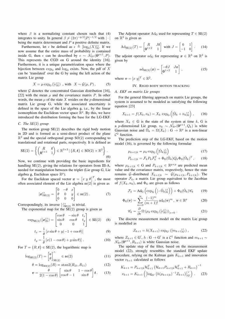
where β is a normalizing constant chosen such that (4)integrates to unity. In general β 6= (2π)−p/2|P |−1/2 with | · |being the matrix determinant and P a positive definite matrix.
Furthermore, let ε be defined as ε , [logG(X)]∨G . If wenow assume that the entire mass of probability is containedinside G, then ε can be described by ε ∼ NRp(0p×1, P ).This represents the CGD on G around the identity [16].Furthermore, it is a unique parametrization space where thebijection between expG and logG exists. Now, the pdf of Xcan be ‘translated’ over the G by using the left action of thematrix Lie group
X = µ expG ([ε]∧G) , with X ∼ G(µ, P ) , (5)
where G denotes the concentrated Gaussian distribution [16],[22] with the mean µ and the covariance matrix P . In otherwords, the mean µ of the state X resides on the p-dimensionalmatrix Lie group G, while the associated uncertainty isdefined in the space of the Lie algebra g, i.e., by the linearisomorphism the Euclidean vector space Rp. By this, we haveintroduced the distribution forming the base for the LG-EKF.
C. The SE(2) group
The motion group SE(2) describes the rigid body motionin 2D and is formed as a semi-direct product of the planeR2 and the special orthogonal group SO(2) corresponding totranslational and rotational parts, respectively. It is defined as
SE(2) =
(R t
01×1 1
)∈ R3×3 | R, t ∈ SO(2)× R2
.
(6)Now, we continue with providing the basic ingredients forhandling SE(2), giving the relations for operators from III-A,needed for manipulation between the triplet (Lie group G, Liealgebra g, Euclidean space Rp).
For the Euclidean spaced vector x =[x y θ
]T, the most
often associated element of the Lie algebra se(2) is given as
[x]∧SE(2) =
0 −θ xθ 0 y0 0 0
∈ se(2) . (7)
Correspondingly, its inverse [·]∨SE(2) is trivial.The exponential map for the SE(2) group is given as
expSE(2)([x]∧G) =
cos θ − sin θ txsin θ cos θ ty
0 0 1
∈ SE(2) (8)
tx =1
θ[x sin θ + y(−1 + cos θ)] (9)
ty =1
θ[x(1− cos θ) + y sin θ)] . (10)
For T = R, t ∈ SE(2), the logarithmic map is
logSE(2)(T ) =
[vθ
]∧
SE(2)∈ se(2) (11)
θ = logSO(2)(R) = atan2(R21, R11) (12)
v =θ
2(1− cos θ)
[sin θ 1− cos θ
cos θ − 1 sin θ
]t . (13)
The Adjoint operator AdG used for representing T ∈ SE(2)on R3 is given as
AdSE(2)(T ) =
[R Jt
01×2 1
]with J =
[0 1−1 0
]. (14)
The adjoint operator adG for representing x ∈ R3 on R3 isgiven by
adSE(2)(x) =
[−θJ Jv01×2 1
], (15)
where v = [x y]T ∈ R2.
IV. RIGID BODY MOTION TRACKING
A. EKF on matrix Lie groups
For the general filtering approach on matrix Lie groups, thesystem is assumed to be modeled as satisfying the followingequation [23]
Xk+1 = f(Xk, nk) = Xk expG
([Ωk + nk]∧G
), (16)
where Xk ∈ G is the state of the system at time k, G isa p-dimensional Lie group, nk ∼ NRp(0p×1, Qk) is whiteGaussian noise and Ωk = Ω(Xk) : G → Rp is a non-linearC2 function.
The prediction step of the LG-EKF, based on the motionmodel (16), is governed by the following formulae
µk+1|k = µk expG
([Ωk]∧G
)(17)
Pk+1|k = FkPkFTk + ΦG(Ωk)QkΦG(Ωk)T , (18)
where µk+1|k ∈ G and Pk+1|k ∈ Rp×p are predicted meanvalue and the covariance matrix, respectively, hence the stateremains G–distributed Xk+1|k ∼ G(µk+1|k, Pk+1|k). Theoperator Fk, a matrix Lie group equivalent to the Jacobianof f(Xk, nk), and ΦG are given as follows
Fk = AdG
(expG
([−Ωk]∧G
))+ ΦG(Ωk)Ck (19)
ΦG(v) =∞∑
m=0
(−1)m
(m+ 1)!adG(v)m , v ∈ Rp (20)
Ck =∂
∂εΩ (µk expG ([ε]∧G))|ε=0 . (21)
The discrete measurement model on the matrix Lie groupis modelled as
Zk+1 = h(Xk+1) expG′ ([mk+1]∧G′) , (22)
where Zk+1 ∈ G′, h : G→ G′ is a C1 function and mk+1 ∼NRq (0q×1, Rk+1) is white Gaussian noise.
The update step of the filter, based on the measurementmodel (22), strongly resembles the standard EKF updateprocedure, relying on the Kalman gain Kk+1 and innovationvector νk+1 calculated as follows
Kk+1 = Pk+1|kHTk+1
(Hk+1Pk+1|kHTk+1 +Rk+1
)−1
νk+1 = Kk+1
([logG′
(h(µk+1|k)−1Zk+1
)]∨G′
). (23)

0 1 20
1
2
x
y
σω = 0
0 1 20
0.5
1
1.5
2
x
σω = 20
0 1 20
1
2
x
σω = 30
0 1 20
1
2
x
σω = 60
0 1 2 3
0
1
2
x
σω = 90
Fig. 2: Each of the subfigures represents an example of two compounding transformations for different levels of rotational uncertainty (givenin blue). The grey circles represent 50 sampled uncertain transformations by employing both translational and rotational uncertainties. Thisparticular situation appears when a robot moves from the current position to the next position associated with the next discrete moment intime, with standard deviation of the rotation σω .
The matrix Hk can be seen as the measurement matrix of thesystem, i.e., a matrix Lie group equivalent to the Jacobian ofh(Xk), and is given as
Hk+1 =∂
∂ε
[logG′
(h(µk+1|k)−1
h(µk+1|k expG ([ε]∧G)
))]∨G |ε=0
.(24)
Finally, having defined all the constituent elements, the updatestep is calculated via
µk+1 = µk+1|k expG ([νk+1]∧G) (25)
Pk+1 = ΦG(νk+1)(Ip×p −Kk+1Hk+1
)Pk+1|kΦG(νk+1)T .
(26)
As in the case of the prediction step, the state Xk+1 ∼G(µk+1, Pk+1) remains G–distributed after the correction aswell. For a more formal derivation of the LG-EKF, theinterested reader is referred to [16].
Since the employment of the SE(2)×R3 follows the similar,but slightly simpler derivation, in the sequel we derive theLG-EKF filter for estimation on the state space modelled asSE(2)2. This approach is in our case applied, but not limited,to the problem of moving object tracking.
B. LG-EKF on SE(2)2
As mentioned previously, we model the state X to evolveon the matrix Lie group G = SE(2)2 which is symbolicallyrepresented by
X =
[Rθ t01×2 1
]
[Rω tv01×2 1
]
=
(Ts
Td
)
G
, (27)
where Ts is the stationary component and Td brings the secondorder dynamics. Note that the matrix Lie group compositionand inversion are simple matrix multiplication and inversion,hence the previous symbolic representation can be used for allthe calculations dealing with operations on G.
The Lie algebra associated to the Lie group G is denotedas g = se(2)2, thereby for x =
[xp xd
]T ∈ R6, where xp =[x y θ
]Tand xd =
[vx vy ω
]T, the following holds
[x]∧G =
[[xp]
∧SE(2)
[xd]∧SE(2)
]=
([xp]
∧SE(2)
[xd]∧SE(2)
)
g
. (28)
The exponential map for such defined G is
expG([x]∧G) =
expSE(2)
([xp]
∧SE(2)
)
expSE(2)
([xd]
∧SE(2)
)
G
. (29)
Now, we have all the necessary ingredients for deriving theterms to be used within the LG-EKF. Several examples of theuncertain transformations following the SE(2)2 motion modelare shown in Fig. 2 (the SE(2) × R3 model would exhibitsimilar behaviour).
1) Prediction: We propose to model the motion (16) of thesystem by
Ω(Xk) =[Tvxk
Tvyk Tωk 0 0 0]T ∈ R6 , (30)
nk =[T 2
2 nxk
T 2
2 nykT 2
2 nωkTnxk
Tnyk Tnωk
]T∈ R6 .
With such a defined motion model, the system is corruptedwith white noise over three separated components, i.e., nxthe noise in the local x direction, ny the noise in the local ydirection and nw as the noise in the rotational component.Given that, the intensity of the noise components acts asacceleration over the associated axes in the system. If thesystem state at the discrete time step k is described withXk ∼ G(µk, Pk), the mean value and the covariance can bepropagated using (17) and (18).
The covariance propagation is more challenging, since itrequires the calculation of (21). For the Lie algebraic errorε ,
[εx εy εθ εvx εvy εω
], we need to set the following
Ω (µk expG ([ε]∧G))
=
∆Tvxk+ ∆T cosωk v1 −∆T sinωk v2
∆Tvyk + ∆T sinωk v1 + ∆T cosωk v2∆Tωk + ∆Tεω
03×1
.
(31)
where
v1 =[εvx sin εω + εvy (cos εω − 1)
]ε−1ω
v2 =[εvx(1− cos εω) + εvy sin εω
]ε−1ω .
(32)
Let Ω1,k, Ω2,k and Ω3,k denote the first three rows of thevector (31), respectively (whereas the last three rows are trivialΩ4,k = Ω5,k = Ω6,k = 0). Even though the multivariate limits∂Ω1,k
∂εω|ε=0 and
∂Ω2,k
∂εω|ε=0 appear involved, their derivation
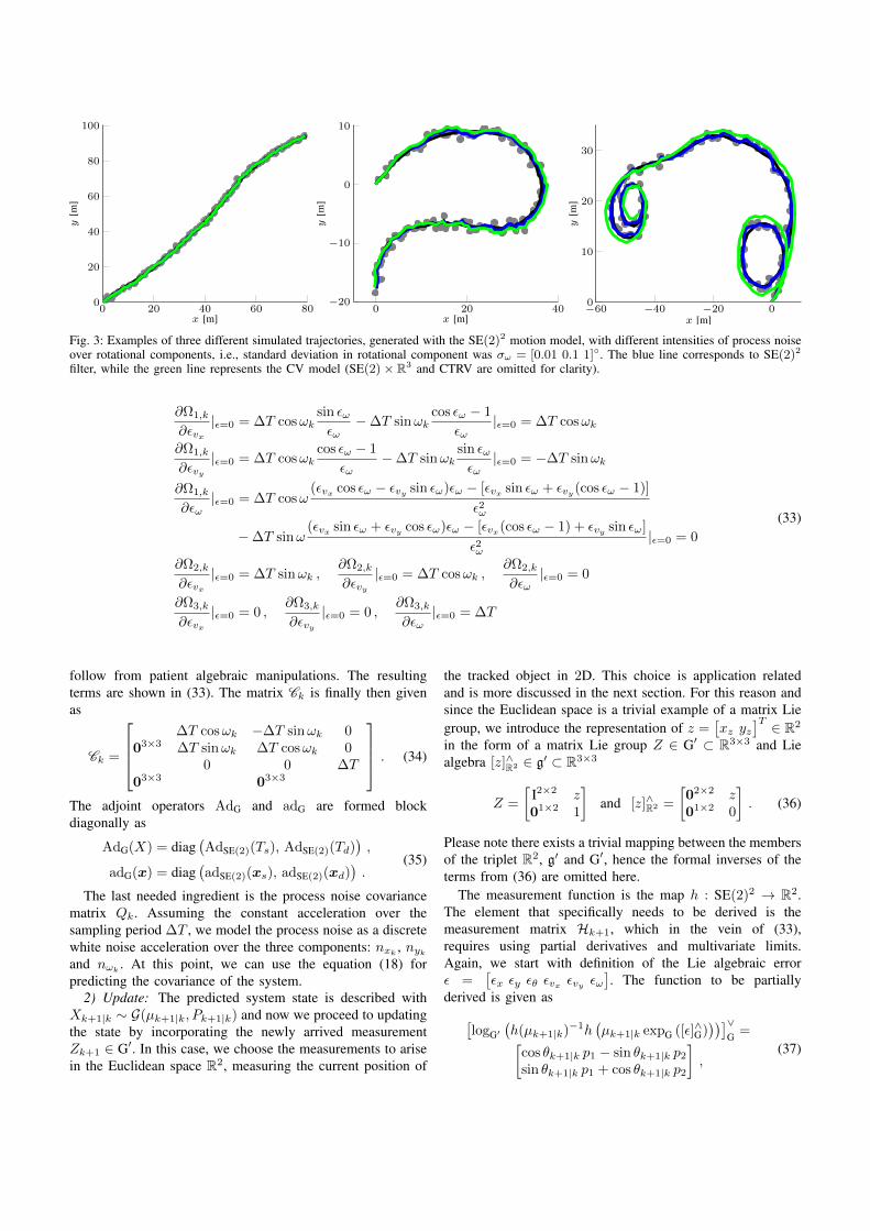
0 20 40 60 800
20
40
60
80
100
x [m]
y[m
]
0 20 40−20
−10
0
10
x [m]y
[m]
−60 −40 −20 00
10
20
30
x [m]
y[m
]
Fig. 3: Examples of three different simulated trajectories, generated with the SE(2)2 motion model, with different intensities of process noiseover rotational components, i.e., standard deviation in rotational component was σω = [0.01 0.1 1]. The blue line corresponds to SE(2)2
filter, while the green line represents the CV model (SE(2)× R3 and CTRV are omitted for clarity).
∂Ω1,k
∂εvx|ε=0 = ∆T cosωk
sin εωεω
−∆T sinωkcos εω − 1
εω|ε=0 = ∆T cosωk
∂Ω1,k
∂εvy|ε=0 = ∆T cosωk
cos εω − 1
εω−∆T sinωk
sin εωεω|ε=0 = −∆T sinωk
∂Ω1,k
∂εω|ε=0 = ∆T cosω
(εvx cos εω − εvy sin εω)εω − [εvx sin εω + εvy (cos εω − 1)]
ε2ω
−∆T sinω(εvx sin εω + εvy cos εω)εω − [εvx(cos εω − 1) + εvy sin εω]
ε2ω|ε=0 = 0
∂Ω2,k
∂εvx|ε=0 = ∆T sinωk ,
∂Ω2,k
∂εvy|ε=0 = ∆T cosωk ,
∂Ω2,k
∂εω|ε=0 = 0
∂Ω3,k
∂εvx|ε=0 = 0 ,
∂Ω3,k
∂εvy|ε=0 = 0 ,
∂Ω3,k
∂εω|ε=0 = ∆T
(33)
follow from patient algebraic manipulations. The resultingterms are shown in (33). The matrix Ck is finally then givenas
Ck =
03×3
∆T cosωk −∆T sinωk 0∆T sinωk ∆T cosωk 0
0 0 ∆T03×3 03×3
. (34)
The adjoint operators AdG and adG are formed blockdiagonally as
AdG(X) = diag(AdSE(2)(Ts), AdSE(2)(Td)
),
adG(x) = diag(adSE(2)(xs), adSE(2)(xd)
).
(35)
The last needed ingredient is the process noise covariancematrix Qk. Assuming the constant acceleration over thesampling period ∆T , we model the process noise as a discretewhite noise acceleration over the three components: nxk
, nykand nωk
. At this point, we can use the equation (18) forpredicting the covariance of the system.
2) Update: The predicted system state is described withXk+1|k ∼ G(µk+1|k, Pk+1|k) and now we proceed to updatingthe state by incorporating the newly arrived measurementZk+1 ∈ G′. In this case, we choose the measurements to arisein the Euclidean space R2, measuring the current position of
the tracked object in 2D. This choice is application relatedand is more discussed in the next section. For this reason andsince the Euclidean space is a trivial example of a matrix Liegroup, we introduce the representation of z =
[xz yz
]T ∈ R2
in the form of a matrix Lie group Z ∈ G′ ⊂ R3×3 and Liealgebra [z]∧R2 ∈ g′ ⊂ R3×3
Z =
[I2×2 z01×2 1
]and [z]∧R2 =
[02×2 z01×2 0
]. (36)
Please note there exists a trivial mapping between the membersof the triplet R2, g′ and G′, hence the formal inverses of theterms from (36) are omitted here.
The measurement function is the map h : SE(2)2 → R2.The element that specifically needs to be derived is themeasurement matrix Hk+1, which in the vein of (33),requires using partial derivatives and multivariate limits.Again, we start with definition of the Lie algebraic errorε =
[εx εy εθ εvx εvy εω
]. The function to be partially
derived is given as
[logG′
(h(µk+1|k)−1h
(µk+1|k expG ([ε]∧G)
))]∨G =[
cos θk+1|k p1 − sin θk+1|k p2sin θk+1|k p1 + cos θk+1|k p2
],
(37)
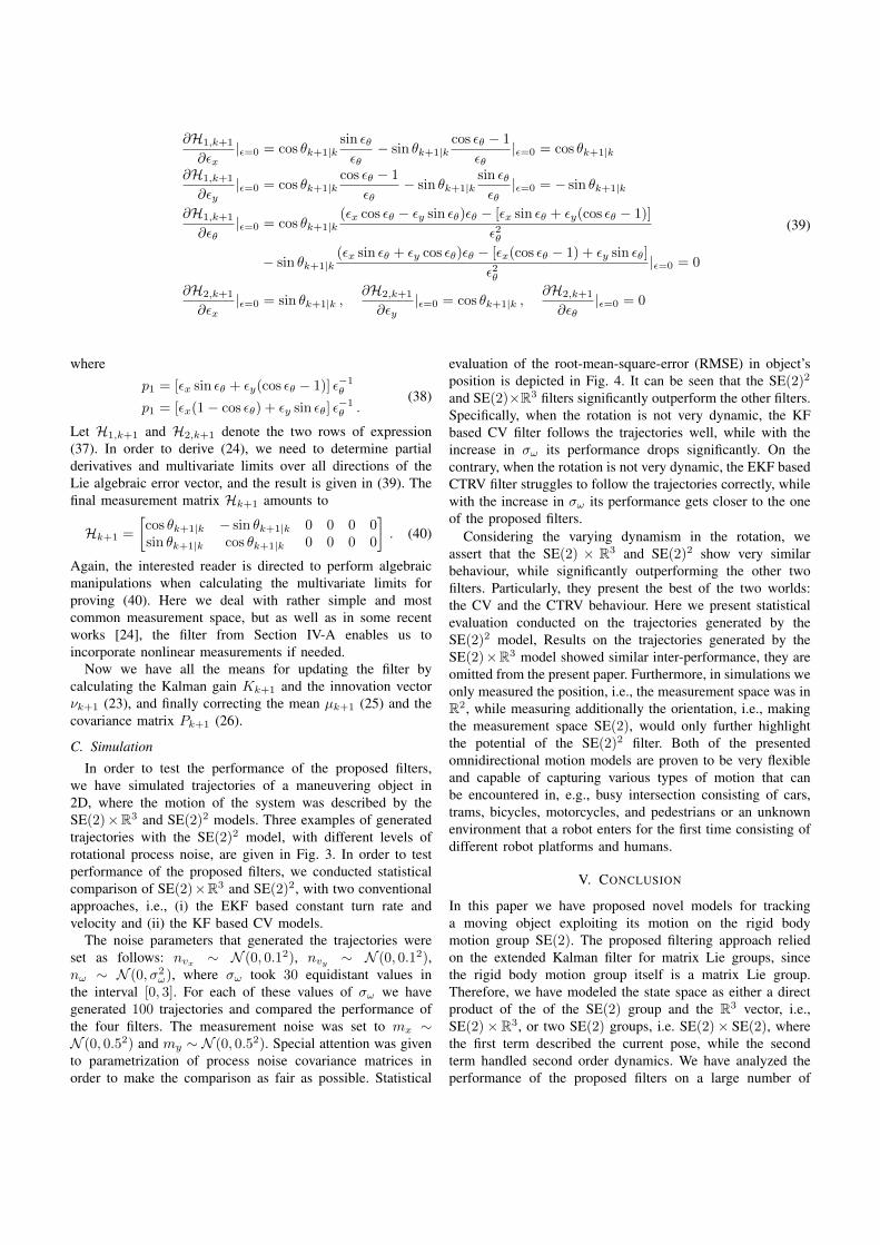
∂H1,k+1
∂εx|ε=0 = cos θk+1|k
sin εθεθ− sin θk+1|k
cos εθ − 1
εθ|ε=0 = cos θk+1|k
∂H1,k+1
∂εy|ε=0 = cos θk+1|k
cos εθ − 1
εθ− sin θk+1|k
sin εθεθ|ε=0 = − sin θk+1|k
∂H1,k+1
∂εθ|ε=0 = cos θk+1|k
(εx cos εθ − εy sin εθ)εθ − [εx sin εθ + εy(cos εθ − 1)]
ε2θ
− sin θk+1|k(εx sin εθ + εy cos εθ)εθ − [εx(cos εθ − 1) + εy sin εθ]
ε2θ|ε=0 = 0
∂H2,k+1
∂εx|ε=0 = sin θk+1|k ,
∂H2,k+1
∂εy|ε=0 = cos θk+1|k ,
∂H2,k+1
∂εθ|ε=0 = 0
(39)
where
p1 = [εx sin εθ + εy(cos εθ − 1)] ε−1θp1 = [εx(1− cos εθ) + εy sin εθ] ε
−1θ .
(38)
Let H1,k+1 and H2,k+1 denote the two rows of expression(37). In order to derive (24), we need to determine partialderivatives and multivariate limits over all directions of theLie algebraic error vector, and the result is given in (39). Thefinal measurement matrix Hk+1 amounts to
Hk+1 =
[cos θk+1|k − sin θk+1|k 0 0 0 0sin θk+1|k cos θk+1|k 0 0 0 0
]. (40)
Again, the interested reader is directed to perform algebraicmanipulations when calculating the multivariate limits forproving (40). Here we deal with rather simple and mostcommon measurement space, but as well as in some recentworks [24], the filter from Section IV-A enables us toincorporate nonlinear measurements if needed.
Now we have all the means for updating the filter bycalculating the Kalman gain Kk+1 and the innovation vectorνk+1 (23), and finally correcting the mean µk+1 (25) and thecovariance matrix Pk+1 (26).
C. Simulation
In order to test the performance of the proposed filters,we have simulated trajectories of a maneuvering object in2D, where the motion of the system was described by theSE(2)×R3 and SE(2)2 models. Three examples of generatedtrajectories with the SE(2)2 model, with different levels ofrotational process noise, are given in Fig. 3. In order to testperformance of the proposed filters, we conducted statisticalcomparison of SE(2)×R3 and SE(2)2, with two conventionalapproaches, i.e., (i) the EKF based constant turn rate andvelocity and (ii) the KF based CV models.
The noise parameters that generated the trajectories wereset as follows: nvx ∼ N (0, 0.12), nvy ∼ N (0, 0.12),nω ∼ N (0, σ2
ω), where σω took 30 equidistant values inthe interval [0, 3]. For each of these values of σω we havegenerated 100 trajectories and compared the performance ofthe four filters. The measurement noise was set to mx ∼N (0, 0.52) and my ∼ N (0, 0.52). Special attention was givento parametrization of process noise covariance matrices inorder to make the comparison as fair as possible. Statistical
evaluation of the root-mean-square-error (RMSE) in object’sposition is depicted in Fig. 4. It can be seen that the SE(2)2
and SE(2)×R3 filters significantly outperform the other filters.Specifically, when the rotation is not very dynamic, the KFbased CV filter follows the trajectories well, while with theincrease in σω its performance drops significantly. On thecontrary, when the rotation is not very dynamic, the EKF basedCTRV filter struggles to follow the trajectories correctly, whilewith the increase in σω its performance gets closer to the oneof the proposed filters.
Considering the varying dynamism in the rotation, weassert that the SE(2) × R3 and SE(2)2 show very similarbehaviour, while significantly outperforming the other twofilters. Particularly, they present the best of the two worlds:the CV and the CTRV behaviour. Here we present statisticalevaluation conducted on the trajectories generated by theSE(2)2 model, Results on the trajectories generated by theSE(2)×R3 model showed similar inter-performance, they areomitted from the present paper. Furthermore, in simulations weonly measured the position, i.e., the measurement space was inR2, while measuring additionally the orientation, i.e., makingthe measurement space SE(2), would only further highlightthe potential of the SE(2)2 filter. Both of the presentedomnidirectional motion models are proven to be very flexibleand capable of capturing various types of motion that canbe encountered in, e.g., busy intersection consisting of cars,trams, bicycles, motorcycles, and pedestrians or an unknownenvironment that a robot enters for the first time consisting ofdifferent robot platforms and humans.
V. CONCLUSION
In this paper we have proposed novel models for trackinga moving object exploiting its motion on the rigid bodymotion group SE(2). The proposed filtering approach reliedon the extended Kalman filter for matrix Lie groups, sincethe rigid body motion group itself is a matrix Lie group.Therefore, we have modeled the state space as either a directproduct of the of the SE(2) group and the R3 vector, i.e.,SE(2)×R3, or two SE(2) groups, i.e. SE(2)× SE(2), wherethe first term described the current pose, while the secondterm handled second order dynamics. We have analyzed theperformance of the proposed filters on a large number of

10−1 100
0.6
0.8
1
1.2
1.4
σω []
posi
tion
RM
SE[m
]
Fig. 4: Performance statistics obtained over 100 generatedtrajectories for 30 different values of σω . We have compared theproposed filter SE(2)2 (blue) and SE(2) × R3 (orange) with theEKF based CTRV (green), KF based CV (red), and measurements(black), where the solid lines corresponds to mean values, whiletransparent areas correspond to one standard deviation (in both +/−directions) of each of the associated RMSEs. We can notice that theSE(2)×R3 and SE(2)2 filters, whose difference is barely noticable,exhibit similar behaviour, outperforming the other two filters.
synthetic trajectories and compared them to (i) the EKFbased constant velocity and turn rate and (ii) the KF basedconstant velocity models. The SE(2)× R3 and SE(2)2 filtersshowed similar performance on the synthetic dataset, and havesignificantly outperformed other well-established approachesfor a wide range of intensities in the rotation component.
Even though the presented work was applied on a trackingproblem, we believe it can serve as a starting point forfurther exploitation of estimation on matrix Lie groups andits applications on different problems. The use of higher orderdynamics may be of special interest for the domain of robotics,as well as for multi-target tracking applications. Furthermore,these techniques could also find application in other rigid bodymotion estimation problems requiring precise pose estimationand higher-order motion.
ACKNOWLEDGMENTS
This work has been supported from the Unity ThroughKnowledge Fund under the project Cooperative Cloudbased Simultaneous Localization and Mapping in DynamicEnvironments (cloudSLAM) and the European Union’sHorizon 2020 research and innovation programme undergrant agreement No 688117 (SafeLog).
REFERENCES
[1] T. D. Barfoot and P. T. Furgale, “Associating Uncertainty With Three-Dimensional Poses for Use in Estimation Problems,” IEEE Transactionson Robotics, vol. 30, no. 3, pp. 679–693, Jun. 2014.
[2] C. Hertzberg, R. Wagner, U. Frese, and L. Schroder, “Integrating GenericSensor Fusion Algorithms with Sound State Representations throughEncapsulation of Manifolds,” Information Fusion, vol. 14, no. 1, pp.57–77, Jul. 2013.
[3] R. M. Murray, Z. Li, and S. S. Sastry, A Mathematical Introduction toRobotic Manipulation. CRC Press, 1994, vol. 29.
[4] F. C. Park, J. E. Bobrow, and S. R. Ploen, “A Lie Group Formulationof Robot Dynamics,” The International Journal of Robotics Research,vol. 14, no. 6, pp. 609–618, 1995.
[5] A. J. Davison, “Real-time simultaneous localisation and mapping with asingle camera,” in International Conference on Computer Vision (ICCV),vol. 2. IEEE, 2003, pp. 1403–1410.
[6] Y. M. Lui, “Advances in matrix manifolds for computer vision,” Imageand Vision Computing, vol. 30, no. 6-7, pp. 380–388, Jun. 2012.
[7] S.-F. Su and C. S. G. Lee, “Manipulation and propagation of uncertaintyand verification of applicability of actions in assembly tasks,” IEEETransactions on Systems, Man, and Cybernetics, vol. 22, no. 6, pp.1376–1389, 1992.
[8] G. Silveira, E. Malis, and P. Rives, “An Efficient Direct Approach toVisual SLAM,” IEEE Transactions on Robotics, vol. 24, no. 5, pp. 969–979, 2008.
[9] W. Park, Y. Wang, and G. S. Chirikjian, “The Path-of-ProbabilityAlgorithm for Steering and Feedback Control of Flexible Needles,” TheInternational Journal of Robotics Research, vol. 29, no. 7, pp. 813–830,2010.
[10] R. A. Srivatsan, M. Travers, and H. Choset, “Using Lie algebra forshape estimation of medical snake robots,” in International Conferenceon Intelligent Robots and Systems (IROS), Chicago, USA, 2014.
[11] A. W. Long, K. C. Wolfe, M. J. Mashner, and G. S. Chirikjian, “TheBanana Distribution is Gaussian : A Localization Study with ExponentialCoordinates,” in Proceedings of Robotics: Science and Systems (RSS),2012.
[12] M. Agrawal, “A lie algebraic approach for consistent pose registrationfor general euclidean motion,” in International Conference on IntelligentRobots and Systems (IROS). IEEE, 2006, pp. 1891–1897.
[13] S. Thrun, W. Burgard, and D. Fox, Probabilistic Robotics. MIT Press,2006.
[14] G. Kurz, I. Gilitschenski, and U. D. Hanebeck, “The partially wrappednormal distribution for SE(2) estimation,” in International Conference onMultisensor Fusion and Information Integration for Intelligent Systems(MFI), 2014.
[15] I. Gilitschenski, G. Kurz, S. J. Julier, and U. D. Hanebeck, “A NewProbability Distribution for Simultaneous Representation of UncertainPosition and Orientation,” in International Conference on InformationFusion (FUSION), 2014.
[16] G. Bourmaud, R. Megret, M. Arnaudon, and A. Giremus, “Continuous-Discrete Extended Kalman Filter on Matrix Lie Groups UsingConcentrated Gaussian Distributions,” Journal of Mathematical Imagingand Vision, vol. 51, no. 1, pp. 209–228, 2015.
[17] Y. Bar-Shalom, T. Kirubarajan, and X.-R. Li, Estimation withApplications to Tracking and Navigation. John Wiley & Sons, Inc.,2002.
[18] R. Schubert, “Evaluating the utility of driving: Toward automateddecision making under uncertainty,” IEEE Transactions on IntelligentTransportation Systems, vol. 13, no. 1, pp. 354–364, 2012.
[19] R. Siegwart and I. R. Nourbakhsh, Introduction to Autonomous MobileRobots. Scituate, MA, USA: Bradford Company, 2004.
[20] G. S. Chirikjian, Stochastic Models, Information Theory, and LieGroups, Volume 2: Analytic Methods and Modern Applications.Springer, 2012.
[21] Y. Wang and G. S. Chirikjian, “Nonparametric Second-Order Theory ofError Propagation on Motion Groups,” International Journal on RoboticResearch, vol. 27, no. 11, pp. 1258–1273, 2008.
[22] K. C. Wolfe, M. Mashner, and G. S. Chirikjian, “Bayesian Fusion onLie Groups,” Journal of Algebraic Statistics, vol. 2, no. 1, pp. 75–97,2011.
[23] G. Bourmaud, R. Megret, A. Giremus, and Y. Berthoumieu, “DiscreteExtended Kalman Filter on Lie Groups,” in European Signal ProcessingConference (EUSIPCO), 2013, pp. 1–5.
[24] G. Chirikjian and M. Kobilarov, “Gaussian Approximation of Non-linearMeasurement Models on Lie Groups .” in Conference on Decision andControl (CDC). IEEE, 2014, pp. 6401–6406.

publications 83
publication 4
J. Ćesić, V. Joukov, I. Petrović and D. Kulić. Full Body Human Motion Estimation on Lie
Groups Using 3D Marker Position Measurements. IEEE-RAS International Conference on
Humanoid Robotics (Humanoids). Cancun, Mexico, 826–833, 2016.
Full Body Human Motion Estimation on Lie Groups Using 3D MarkerPosition Measurements
Josip Cesic∗, Vladimir Joukov‡, Ivan Petrovic∗ and Dana Kulic‡
Abstract— This paper proposes a new algorithm for fullbody human motion estimation using 3D marker positionmeasurements. The joints are represented with Lie groupmembers, including special orthogonal groups SO(2) andSO(3), and a special euclidean group SE(3). We employ theLie Group Extended Kalman Filter (LG-EKF) for stochasticinference on groups, thus explicitly accounting for thenon-euclidean geometry of the state space, and provide thederivation of the LG-EKF recursion for articulated motionestimation. We evaluate the performance of the proposedalgorithm in both simulation and on real-world motion capturedata, comparing it with the Euler angles based EKF. Theresults show that the proposed filter significantly outperformsthe Euler angles based EKF, since it estimates human motionmore accurately and is not affected by gimbal lock.
I. INTRODUCTION
Human bodies have evolved to perform complexmanipulation and locomotion tasks. We are able toaccomplish very intricate movements, carry light and heavyloads, achieve energy efficient locomotion at various speeds,reject disturbances, and adapt to environment constraints.Inspired by the human body, robotics researchers aim todevelop systems with similar capabilities. To design ahumanoid that can perform as well as a person, researchersmust first capture and analyze human motion. Accuratepose estimation allows the design of controllers to simulatehuman like movements on a robot through motion re-targeting and imitation learning. In human-robot interactionthe participant’s pose must be known to guarantee safetyand to allow collaborative tasks. Finally, to improve theperformance of assistive devices in rehabilitation or toenhance user’s capabilities with an exoskeleton, the systemmust be able to reproduce human like movements [1].
Optical motion capture is a method to record themovements from body worn markers observed by multiplecameras. The 3D positions of the markers are extractedfrom the images using the relative positions of the camerasto each other and are analyzed to compute the pose.
Typically, a kinematic model of the participant is definedbased on anthropomorphic tables or by measurement
This work has been supported from the Unity Through Knowledge Fundunder the project Cooperative Cloud based Simultaneous Localization andMapping in Dynamic Environments (cloudSLAM) and by the Ministry ofScience, Education and Sports of the Republic of Croatia under the grantCenter of Research Excellence for Data Science and Cooperative Systems(CoE ACROSS).
∗ Josip Cesic and Ivan Petrovic are with the University ofZagreb, Faculty of Electrical Engineering and Computing, Laboratory forAutonomous Systems and Mobile Robotics, Croatia. [email protected],[email protected]
‡ Vladimir Joukov and Dana Kulic are with the University of Waterloo,Department of Electrical and Computer Engineering, Adaptive SystemsLaboratory, Canada. [email protected], [email protected]
and markers are assumed rigidly attached to the skeletonlinks. Unfortunately, for a full body skeletal model, thereis no closed form solution for the inverse kinematics(IK). Differentiating the positions of the attached markerswith respect to the joint angles and forming a Jacobianmatrix allows to iteratively solve for joint angles using thepseudoinverse of the Jacobian. In singular configurationsthe Jacobian is not invertible. It is possible to include anon-zero damping constant in the least squares minimizationto maintain full rank; various damping factors have beenproposed [2].
The Jacobian inverse based methods do not account forstochastic error in marker position measurements, are greatlyaffected by outlier measurements, and are not capable ofpredicting future poses. By treating the skeleton pose as astate and 3D marker positions as measurements, recursivestochastic estimators can be used to help reduce the effectof stochastic marker position errors. Including the jointpositions, velocities, and accelerations in the motion modelof the filter helps to maintain correct pose estimate duringshort term occlusions. Various stochastic filters have beenproposed for IK, such as the Smart Sampling Kalman Filter[3] and the Unscented Kalman Filter [4]. The filteringapproach can even be used to perform estimation fromunlabeled markers [5]. Bonnet et al. modelled not onlykinematics but also the dynamics of a human body withinan EKF to estimate the pose and dynamic parameters [6].
In the aforementioned methods the kinematic models arerigid links connected with joints that may be rotational,translational, or spherical. All of these formulations arerepresentations of transformations in the euclidean space.However, human motion and many other types of motionof interest in robotics do not occur in Euclidean space, butrather arise on curved geometries often called manifolds. Byusing the manifold representations, the overall performanceof wide variety of applications can be significantly improved[7]–[9]. In particular, the attitude of an object can bemodelled as a special orthogonal group SO(n), n = 2, 3,while the pose can be modelled as a special euclideangroup SE(n), n = 2, 3 [7]. Notably, both SO(n) and SE(n)belong to a family of matrix Lie groups. Recently, severaltheoretically rigorous approaches for filtering on manifoldshave been proposed. In [10] the authors proposed an EKFable to perform estimation respecting the geometry of matrixLie groups. Alongside, the unscented transform-based [11]and the particle-based [12] approaches have also attractedsignificant attention.
The benefit of manifolds for human action recognitionhas already been explored in the literature. In [13] the
2016 IEEE-RAS 16th International Conference onHumanoid Robots (Humanoids)Cancun, Mexico, Nov 15-17, 2016
978-1-5090-4718-5/16/$31.00 ©2016 IEEE 826
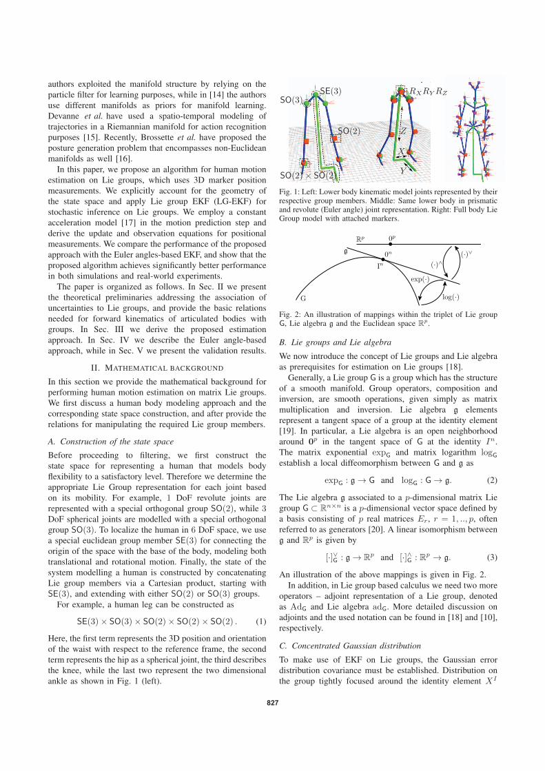
authors exploited the manifold structure by relying on theparticle filter for learning purposes, while in [14] the authorsuse different manifolds as priors for manifold learning.Devanne et al. have used a spatio-temporal modeling oftrajectories in a Riemannian manifold for action recognitionpurposes [15]. Recently, Brossette et al. have proposed theposture generation problem that encompasses non-Euclideanmanifolds as well [16].
In this paper, we propose an algorithm for human motionestimation on Lie groups, which uses 3D marker positionmeasurements. We explicitly account for the geometry ofthe state space and apply Lie group EKF (LG-EKF) forstochastic inference on Lie groups. We employ a constantacceleration model [17] in the motion prediction step andderive the update and observation equations for positionalmeasurements. We compare the performance of the proposedapproach with the Euler angles-based EKF, and show that theproposed algorithm achieves significantly better performancein both simulations and real-world experiments.
The paper is organized as follows. In Sec. II we presentthe theoretical preliminaries addressing the association ofuncertainties to Lie groups, and provide the basic relationsneeded for forward kinematics of articulated bodies withgroups. In Sec. III we derive the proposed estimationapproach. In Sec. IV we describe the Euler angle-basedapproach, while in Sec. V we present the validation results.
II. MATHEMATICAL BACKGROUND
In this section we provide the mathematical background forperforming human motion estimation on matrix Lie groups.We first discuss a human body modeling approach and thecorresponding state space construction, and after provide therelations for manipulating the required Lie group members.
A. Construction of the state space
Before proceeding to filtering, we first construct thestate space for representing a human that models bodyflexibility to a satisfactory level. Therefore we determine theappropriate Lie Group representation for each joint basedon its mobility. For example, 1 DoF revolute joints arerepresented with a special orthogonal group SO(2), while 3DoF spherical joints are modelled with a special orthogonalgroup SO(3). To localize the human in 6 DoF space, we usea special euclidean group member SE(3) for connecting theorigin of the space with the base of the body, modeling bothtranslational and rotational motion. Finally, the state of thesystem modelling a human is constructed by concatenatingLie group members via a Cartesian product, starting withSE(3), and extending with either SO(2) or SO(3) groups.
For example, a human leg can be constructed as
SE(3) × SO(3) × SO(2) × SO(2) × SO(2) . (1)
Here, the first term represents the 3D position and orientationof the waist with respect to the reference frame, the secondterm represents the hip as a spherical joint, the third describesthe knee, while the last two represent the two dimensionalankle as shown in Fig. 1 (left).
SO(2) × SO(2)
SO(2)
SE(3)SO(3)
Z
X
Y
RXRY RZZ
Fig. 1: Left: Lower body kinematic model joints represented by theirrespective group members. Middle: Same lower body in prismaticand revolute (Euler angle) joint representation. Right: Full body LieGroup model with attached markers.
Fig. 2: An illustration of mappings within the triplet of Lie groupG, Lie algebra g and the Euclidean space Rp.
B. Lie groups and Lie algebra
We now introduce the concept of Lie groups and Lie algebraas prerequisites for estimation on Lie groups [18].
Generally, a Lie group G is a group which has the structureof a smooth manifold. Group operators, composition andinversion, are smooth operations, given simply as matrixmultiplication and inversion. Lie algebra g elementsrepresent a tangent space of a group at the identity element[19]. In particular, a Lie algebra is an open neighborhoodaround 0p in the tangent space of G at the identity In.The matrix exponential expG and matrix logarithm logGestablish a local diffeomorphism between G and g as
expG : g → G and logG : G → g. (2)
The Lie algebra g associated to a p-dimensional matrix Liegroup G ⊂ Rn×n is a p-dimensional vector space defined bya basis consisting of p real matrices Er, r = 1, .., p, oftenreferred to as generators [20]. A linear isomorphism betweeng and Rp is given by
[·]∨G : g → Rp and [·]∧G : Rp → g. (3)
An illustration of the above mappings is given in Fig. 2.In addition, in Lie group based calculus we need two more
operators – adjoint representation of a Lie group, denotedas AdG and Lie algebra adG. More detailed discussion onadjoints and the used notation can be found in [18] and [10],respectively.
C. Concentrated Gaussian distribution
To make use of EKF on Lie groups, the Gaussian errordistribution covariance must be established. Distribution onthe group tightly focused around the identity element XI
827

can be expressed on the Lie algebra [21] with probabilitydensity function given as
p(XI) = β exp
(−1
2[logG(XI)]∨
T
G P−1[logG(XI)]∨G
),
where β is a normalizing constant and P is a positive definitematrix. If ε [logG(XI)]∨G is tightly focused, it can bedescribed with a classical Gaussian ε ∼ NRp(0p×1, P ). Thedistribution of random variable XI can be translated overG by using the left action of the Lie group, and finally arandom variable X can be seen as
X = μ expG (ε∧G) , with X ∼ G(μ, P ) , (4)
where G denotes the so called concentrated Gaussiandistribution (CGD) [21]. For a more formal introduction,the interested reader is referred to [18].
D. Special orthogonal group SO(2)
The SO(2) group represents a rotation around a single axis:
SO(2) =X ⊂ R2×2 | XTX = I, det(X) = 1
. (5)
For a euclidean space vector consisting of an angle x = φ,the Lie algebra so(2), is given as
x∧SO(2) =
[0 −φφ 0
]∈ so(2) . (6)
where (·)∧SO(2) : R1 → so(2). Its inverse, (·)∨SO(2) : so(2) →R1, follows trivially from relation (6). The exponential forSO(2), performing expSO(2) : so(2) → SO(2), is given as
expSO(2)(x∧SO(2)) =
[cos φ − sin φsin φ cos φ
], (7)
while the inverse operator, logSO(2) : SO(2) → so(2), canbe evaluated from (7). Due to the commutativity of SO(2),the adjoint operators are given as
AdSO(2)(X) = 1 and adSO(2)(x) = 0 . (8)
These properties will greatly simplify the LG-EKF formulae.
E. Special orthogonal group SO(3)
The SO(3) group represents an orientation of a rigid bodyin 3D space, and is defined as
SO(3) =X ⊂ R3×3 | XTX = I, det(X) = 1
. (9)
For a euclidean joint space vector x = [φ1 φ2 φ3]T, the Lie
algebra so(3) is given as a skew symmetric matrix
x∧SO(3) =
⎡⎣
0 −φ3 φ2
φ3 0 −φ1
−φ2 φ1 0
⎤⎦ ∈ so(3) . (10)
where (·)∧SO(3) : R3 → so(3). Its inverse, (·)∨SO(3) : so(3) →R3, follows trivially from (10). The exponential for SO(3),performing mapping expSO(3) : so(3) → SO(3), is given as
expSO(3)(x∧SO(3)) = cos(|x|)I3+
+ (1 − cos(|x|))xxT
|x|2 + sin(|x|)x∧SO(3)
|x| .(11)
The logarithm, performing mapping logSO(3) : SO(3) →so(3), is given as
logSO(3)(X) =θ
2 sin(θ)(X − XT)
s.t. 1 + 2 cos(θ) = Tr(X)θ = 0 −π < θ < π
θ = 0 log(X) = 0.
(12)
The adjoints AdSO(3) and adSO(3) are respectively given as
AdSO(3)(X) = X and adSO(3)(x) = x∧SO(3) . (13)
F. Special euclidean group SE(3)
The group SE(3) describes 6 DoF rigid body pose and isformed as a semi-direct product of the euclidean space vectorR3 and the special orthogonal group SO(3)1, correspondingto translational and rotational parts, respectively. This groupis defined as
SE(3) =
(R t0 1
)⊂ R4×4 | R, t ∈ SO(3) × R3
.
For a euclidean space vector representing the pose of a rigidbody consisting of a 3DoF position vector t and a 3DoForientation vector φ, where x = [t φ]T, the Lie algebra se(3)is
x∧SE(3) =
[φ∧SO(3) t
0 0
]∈ se(3) . (14)
where (·)∧SE(3) : R6 → se(3). Its inverse, (·)∨SE(3) : se(3) →R6, follows trivially from (14). The exponential for SE(3),performing mapping expSE(3) : se(3) → SE(3), is given as
expSE(3)(x∧SE(3)) =
[C Lt0 1
](15)
C = expSO(3)(φ∧SO(3))
L =sin(|φ|)
|φ| I3 + (1 − sin(|φ|)|φ| )
φφT
|φ|2 +1 − cos(|φ|)
|φ|2 φ∧SO(3).
The logarithm, performing mapping logSE(3) : SE(3) →se(3), is calculated by deconstructing X , and determiningφ by using (12). Then, from (15) we can determine t.
In order to determine the adjoints for SE(3), we need todeconstruct the state X ∈ SE(3) and vector x ∈ R6. Firstly,we extract the rotation part C and translation part t from X ,and secondly, we split the translation part t and orientationpart φ from x. Then, the adjoints AdSE(3) and adSE(3) are
AdSE(3)(X) =
[C tC0 C
], adSE(3)(x) =
[φ∧SO(3) t∧SO(3)
0 φ∧SO(3)
].
We next present the new human motion estimation methodbased on the LG-EKF.
1The euclidean space can be formed only by employing direct product,while other ways to concatenate Lie groups also exist, i.e., semi-directproduct, twisted product, etc.
828
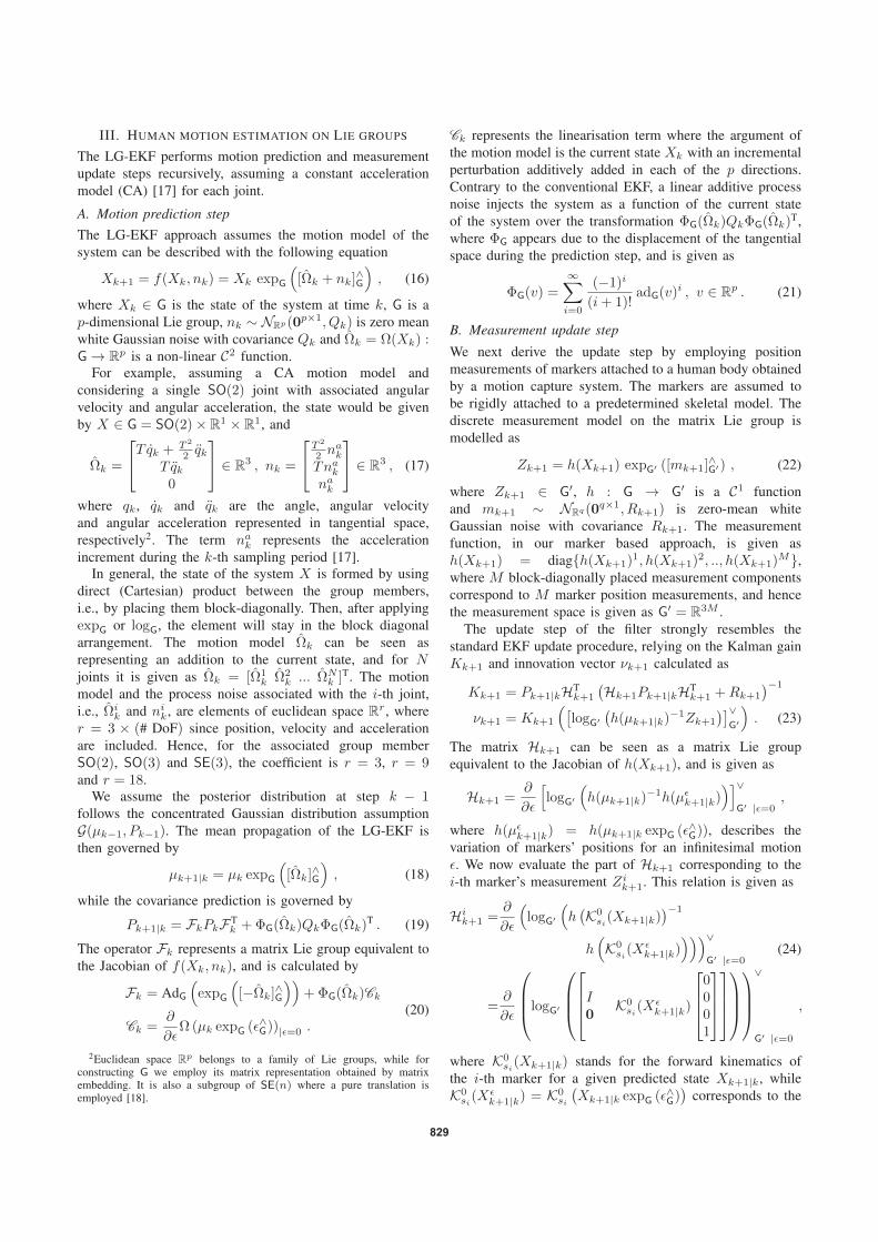
III. HUMAN MOTION ESTIMATION ON LIE GROUPS
The LG-EKF performs motion prediction and measurementupdate steps recursively, assuming a constant accelerationmodel (CA) [17] for each joint.
A. Motion prediction stepThe LG-EKF approach assumes the motion model of thesystem can be described with the following equation
Xk+1 = f(Xk, nk) = Xk expG
([Ωk + nk]
∧G
), (16)
where Xk ∈ G is the state of the system at time k, G is ap-dimensional Lie group, nk ∼ NRp(0p×1, Qk) is zero meanwhite Gaussian noise with covariance Qk and Ωk = Ω(Xk) :G → Rp is a non-linear C2 function.
For example, assuming a CA motion model andconsidering a single SO(2) joint with associated angularvelocity and angular acceleration, the state would be givenby X ∈ G = SO(2) × R1 × R1, and
Ωk =
⎡⎣
T qk + T 2
2 qkT qk0
⎤⎦ ∈ R3 , nk =
⎡⎣
T 2
2 nak
Tnak
nak
⎤⎦ ∈ R3 , (17)
where qk, qk and qk are the angle, angular velocityand angular acceleration represented in tangential space,respectively2. The term na
k represents the accelerationincrement during the k-th sampling period [17].
In general, the state of the system X is formed by usingdirect (Cartesian) product between the group members,i.e., by placing them block-diagonally. Then, after applyingexpG or logG, the element will stay in the block diagonalarrangement. The motion model Ωk can be seen asrepresenting an addition to the current state, and for Njoints it is given as Ωk = [Ω1
k Ω2k ... ΩN
k ]T. The motionmodel and the process noise associated with the i-th joint,i.e., Ωi
k and nik, are elements of euclidean space Rr, where
r = 3 × (# DoF) since position, velocity and accelerationare included. Hence, for the associated group memberSO(2), SO(3) and SE(3), the coefficient is r = 3, r = 9and r = 18.
We assume the posterior distribution at step k − 1follows the concentrated Gaussian distribution assumptionG(μk−1, Pk−1). The mean propagation of the LG-EKF isthen governed by
μk+1|k = μk expG
([Ωk]
∧G
), (18)
while the covariance prediction is governed by
Pk+1|k = FkPkFTk + ΦG(Ωk)QkΦG(Ωk)
T . (19)
The operator Fk represents a matrix Lie group equivalent tothe Jacobian of f(Xk, nk), and is calculated by
Fk = AdG
(expG
([−Ωk]
∧G
))+ ΦG(Ωk)Ck
Ck =∂
∂εΩ (μk expG (ε∧G))|ε=0 .
(20)
2Euclidean space Rp belongs to a family of Lie groups, while forconstructing G we employ its matrix representation obtained by matrixembedding. It is also a subgroup of SE(n) where a pure translation isemployed [18].
Ck represents the linearisation term where the argument ofthe motion model is the current state Xk with an incrementalperturbation additively added in each of the p directions.Contrary to the conventional EKF, a linear additive processnoise injects the system as a function of the current stateof the system over the transformation ΦG(Ωk)QkΦG(Ωk)
T,where ΦG appears due to the displacement of the tangentialspace during the prediction step, and is given as
ΦG(v) =∞∑
i=0
(−1)i
(i + 1)!adG(v)i , v ∈ Rp . (21)
B. Measurement update step
We next derive the update step by employing positionmeasurements of markers attached to a human body obtainedby a motion capture system. The markers are assumed tobe rigidly attached to a predetermined skeletal model. Thediscrete measurement model on the matrix Lie group ismodelled as
Zk+1 = h(Xk+1) expG′ ([mk+1]∧G′) , (22)
where Zk+1 ∈ G′, h : G → G′ is a C1 functionand mk+1 ∼ NRq (0q×1, Rk+1) is zero-mean whiteGaussian noise with covariance Rk+1. The measurementfunction, in our marker based approach, is given ash(Xk+1) = diagh(Xk+1)
1, h(Xk+1)2, .., h(Xk+1)
M,where M block-diagonally placed measurement componentscorrespond to M marker position measurements, and hencethe measurement space is given as G′ = R3M .
The update step of the filter strongly resembles thestandard EKF update procedure, relying on the Kalman gainKk+1 and innovation vector νk+1 calculated as
Kk+1 = Pk+1|kHTk+1
(Hk+1Pk+1|kHT
k+1 + Rk+1
)−1
νk+1 = Kk+1
([logG′
(h(μk+1|k)
−1Zk+1
)]∨G′
). (23)
The matrix Hk+1 can be seen as a matrix Lie groupequivalent to the Jacobian of h(Xk+1), and is given as
Hk+1 =∂
∂ε
[logG′
(h(μk+1|k)
−1h(μεk+1|k)
)]∨G′ |ε=0
,
where h(μεk+1|k) = h(μk+1|k expG (ε∧G)), describes the
variation of markers’ positions for an infinitesimal motionε. We now evaluate the part of Hk+1 corresponding to thei-th marker’s measurement Zi
k+1. This relation is given as
Hik+1 =
∂
∂ε
(logG′
(h(K0
si(Xk+1|k))−1
h(K0
si(Xεk+1|k)
)))∨G′ |ε=0
(24)
=∂
∂ε
⎛⎜⎜⎝logG′
⎛⎜⎜⎝
⎡⎢⎢⎣
I0
K0si(X
εk+1|k)
⎡⎢⎢⎣
0001
⎤⎥⎥⎦
⎤⎥⎥⎦
⎞⎟⎟⎠
⎞⎟⎟⎠
∨
G′ |ε=0
,
where K0si(Xk+1|k) stands for the forward kinematics of
the i-th marker for a given predicted state Xk+1|k, whileK0
si(Xεk+1|k) = K0
si
(Xk+1|k expG (ε∧G)
)corresponds to the
829
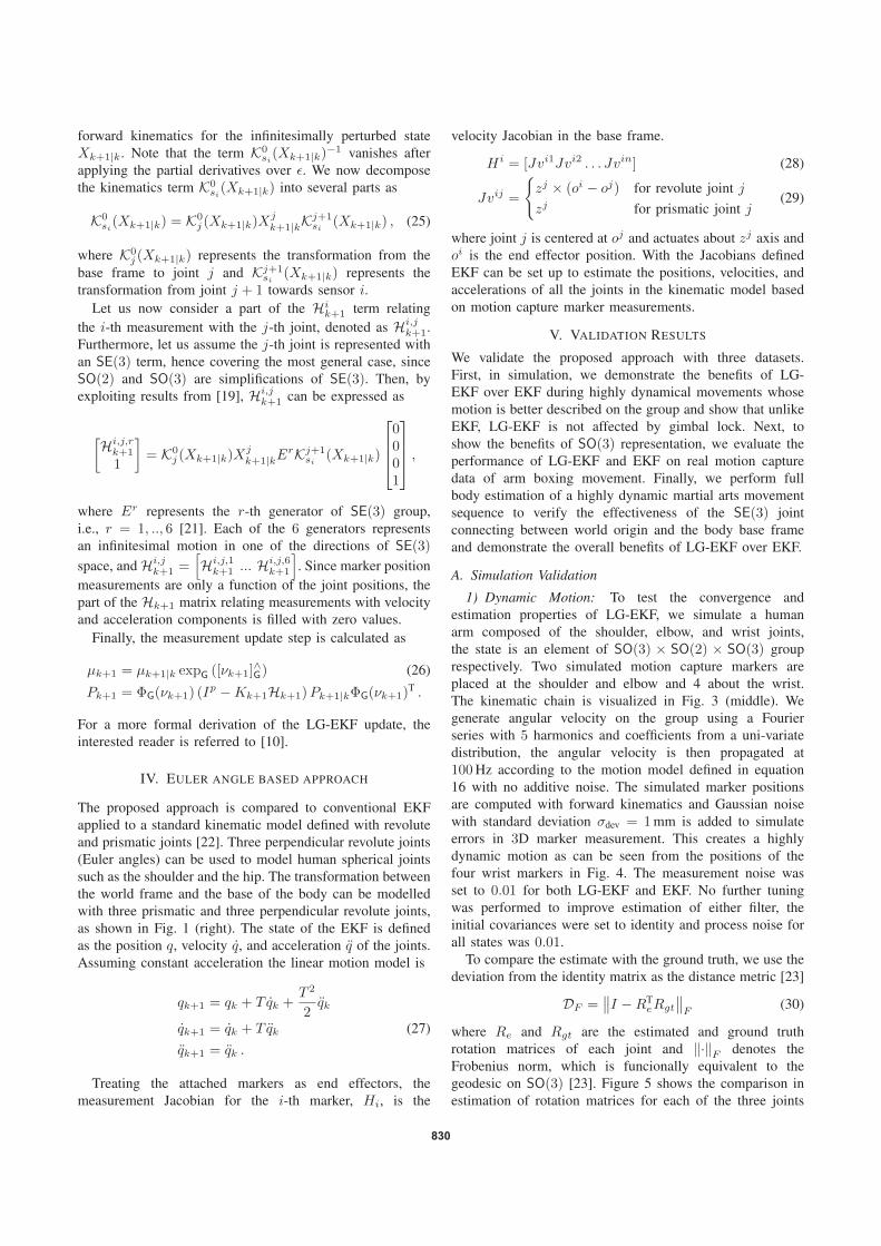
forward kinematics for the infinitesimally perturbed stateXk+1|k. Note that the term K0
si(Xk+1|k)−1 vanishes afterapplying the partial derivatives over ε. We now decomposethe kinematics term K0
si(Xk+1|k) into several parts as
K0si(Xk+1|k) = K0
j (Xk+1|k)Xjk+1|kKj+1
si (Xk+1|k) , (25)
where K0j (Xk+1|k) represents the transformation from the
base frame to joint j and Kj+1si (Xk+1|k) represents the
transformation from joint j + 1 towards sensor i.Let us now consider a part of the Hi
k+1 term relatingthe i-th measurement with the j-th joint, denoted as Hi,j
k+1.Furthermore, let us assume the j-th joint is represented withan SE(3) term, hence covering the most general case, sinceSO(2) and SO(3) are simplifications of SE(3). Then, byexploiting results from [19], Hi,j
k+1 can be expressed as
[Hi,j,r
k+1
1
]= K0
j (Xk+1|k)Xjk+1|kE
rKj+1si (Xk+1|k)
⎡⎢⎢⎣
0001
⎤⎥⎥⎦ ,
where Er represents the r-th generator of SE(3) group,i.e., r = 1, .., 6 [21]. Each of the 6 generators representsan infinitesimal motion in one of the directions of SE(3)
space, and Hi,jk+1 =
[Hi,j,1
k+1 ... Hi,j,6k+1
]. Since marker position
measurements are only a function of the joint positions, thepart of the Hk+1 matrix relating measurements with velocityand acceleration components is filled with zero values.
Finally, the measurement update step is calculated as
μk+1 = μk+1|k expG ([νk+1]∧G) (26)
Pk+1 = ΦG(νk+1) (Ip − Kk+1Hk+1) Pk+1|kΦG(νk+1)T .
For a more formal derivation of the LG-EKF update, theinterested reader is referred to [10].
IV. EULER ANGLE BASED APPROACH
The proposed approach is compared to conventional EKFapplied to a standard kinematic model defined with revoluteand prismatic joints [22]. Three perpendicular revolute joints(Euler angles) can be used to model human spherical jointssuch as the shoulder and the hip. The transformation betweenthe world frame and the base of the body can be modelledwith three prismatic and three perpendicular revolute joints,as shown in Fig. 1 (right). The state of the EKF is definedas the position q, velocity q, and acceleration q of the joints.Assuming constant acceleration the linear motion model is
qk+1 = qk + T qk +T 2
2qk
qk+1 = qk + T qk (27)qk+1 = qk .
Treating the attached markers as end effectors, themeasurement Jacobian for the i-th marker, Hi, is the
velocity Jacobian in the base frame.
Hi = [Jvi1Jvi2 . . . Jvin] (28)
Jvij =
zj × (oi − oj) for revolute joint j
zj for prismatic joint j(29)
where joint j is centered at oj and actuates about zj axis andoi is the end effector position. With the Jacobians definedEKF can be set up to estimate the positions, velocities, andaccelerations of all the joints in the kinematic model basedon motion capture marker measurements.
V. VALIDATION RESULTS
We validate the proposed approach with three datasets.First, in simulation, we demonstrate the benefits of LG-EKF over EKF during highly dynamical movements whosemotion is better described on the group and show that unlikeEKF, LG-EKF is not affected by gimbal lock. Next, toshow the benefits of SO(3) representation, we evaluate theperformance of LG-EKF and EKF on real motion capturedata of arm boxing movement. Finally, we perform fullbody estimation of a highly dynamic martial arts movementsequence to verify the effectiveness of the SE(3) jointconnecting between world origin and the body base frameand demonstrate the overall benefits of LG-EKF over EKF.
A. Simulation Validation
1) Dynamic Motion: To test the convergence andestimation properties of LG-EKF, we simulate a humanarm composed of the shoulder, elbow, and wrist joints,the state is an element of SO(3) × SO(2) × SO(3) grouprespectively. Two simulated motion capture markers areplaced at the shoulder and elbow and 4 about the wrist.The kinematic chain is visualized in Fig. 3 (middle). Wegenerate angular velocity on the group using a Fourierseries with 5 harmonics and coefficients from a uni-variatedistribution, the angular velocity is then propagated at100 Hz according to the motion model defined in equation16 with no additive noise. The simulated marker positionsare computed with forward kinematics and Gaussian noisewith standard deviation σdev = 1 mm is added to simulateerrors in 3D marker measurement. This creates a highlydynamic motion as can be seen from the positions of thefour wrist markers in Fig. 4. The measurement noise wasset to 0.01 for both LG-EKF and EKF. No further tuningwas performed to improve estimation of either filter, theinitial covariances were set to identity and process noise forall states was 0.01.
To compare the estimate with the ground truth, we use thedeviation from the identity matrix as the distance metric [23]
DF =∥∥I − RT
eRgt
∥∥F
(30)
where Re and Rgt are the estimated and ground truthrotation matrices of each joint and ‖·‖F denotes theFrobenius norm, which is funcionally equivalent to thegeodesic on SO(3) [23]. Figure 5 shows the comparison inestimation of rotation matrices for each of the three joints
830
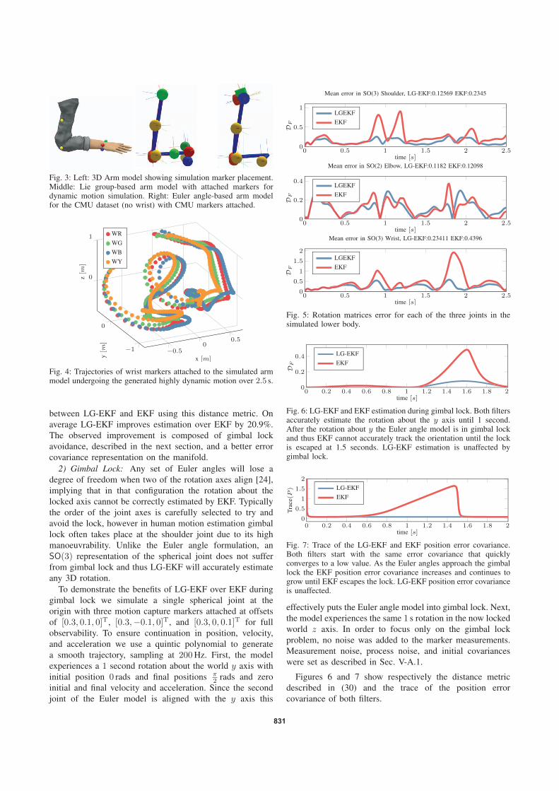
Fig. 3: Left: 3D Arm model showing simulation marker placement.Middle: Lie group-based arm model with attached markers fordynamic motion simulation. Right: Euler angle-based arm modelfor the CMU dataset (no wrist) with CMU markers attached.
−0.50
0.5
−1
0
0
1
x [m]y[m
]
z[m
]
WRWGWBWY
Fig. 4: Trajectories of wrist markers attached to the simulated armmodel undergoing the generated highly dynamic motion over 2.5 s.
between LG-EKF and EKF using this distance metric. Onaverage LG-EKF improves estimation over EKF by 20.9%.The observed improvement is composed of gimbal lockavoidance, described in the next section, and a better errorcovariance representation on the manifold.
2) Gimbal Lock: Any set of Euler angles will lose adegree of freedom when two of the rotation axes align [24],implying that in that configuration the rotation about thelocked axis cannot be correctly estimated by EKF. Typicallythe order of the joint axes is carefully selected to try andavoid the lock, however in human motion estimation gimballock often takes place at the shoulder joint due to its highmanoeuvrability. Unlike the Euler angle formulation, anSO(3) representation of the spherical joint does not sufferfrom gimbal lock and thus LG-EKF will accurately estimateany 3D rotation.
To demonstrate the benefits of LG-EKF over EKF duringgimbal lock we simulate a single spherical joint at theorigin with three motion capture markers attached at offsetsof [0.3, 0.1, 0]T, [0.3, −0.1, 0]T, and [0.3, 0, 0.1]T for fullobservability. To ensure continuation in position, velocity,and acceleration we use a quintic polynomial to generatea smooth trajectory, sampling at 200 Hz. First, the modelexperiences a 1 second rotation about the world y axis withinitial position 0 rads and final positions π
2 rads and zeroinitial and final velocity and acceleration. Since the secondjoint of the Euler model is aligned with the y axis this
0 0.5 1 1.5 2 2.50
0.5
1
time [s]
DF
Mean error in SO(3) Shoulder, LG-EKF:0.12569 EKF:0.2345
LGEKFEKF
0 0.5 1 1.5 2 2.50
0.2
0.4
time [s]
DF
Mean error in SO(2) Elbow, LG-EKF:0.1182 EKF:0.12098
LGEKFEKF
0 0.5 1 1.5 2 2.50
0.5
1
1.5
2
time [s]
DF
Mean error in SO(3) Wrist, LG-EKF:0.23411 EKF:0.4396
LGEKFEKF
Fig. 5: Rotation matrices error for each of the three joints in thesimulated lower body.
0 0.2 0.4 0.6 0.8 1 1.2 1.4 1.6 1.8 20
0.2
0.4
time [s]
DF
LG-EKFEKF
Fig. 6: LG-EKF and EKF estimation during gimbal lock. Both filtersaccurately estimate the rotation about the y axis until 1 second.After the rotation about y the Euler angle model is in gimbal lockand thus EKF cannot accurately track the orientation until the lockis escaped at 1.5 seconds. LG-EKF estimation is unaffected bygimbal lock.
0 0.2 0.4 0.6 0.8 1 1.2 1.4 1.6 1.8 20
0.5
1
1.5
2
time [s]
Trac
e(P) LG-EKF
EKF
Fig. 7: Trace of the LG-EKF and EKF position error covariance.Both filters start with the same error covariance that quicklyconverges to a low value. As the Euler angles approach the gimballock the EKF position error covariance increases and continues togrow until EKF escapes the lock. LG-EKF position error covarianceis unaffected.
effectively puts the Euler angle model into gimbal lock. Next,the model experiences the same 1 s rotation in the now lockedworld z axis. In order to focus only on the gimbal lockproblem, no noise was added to the marker measurements.Measurement noise, process noise, and initial covarianceswere set as described in Sec. V-A.1.
Figures 6 and 7 show respectively the distance metricdescribed in (30) and the trace of the position errorcovariance of both filters.
831
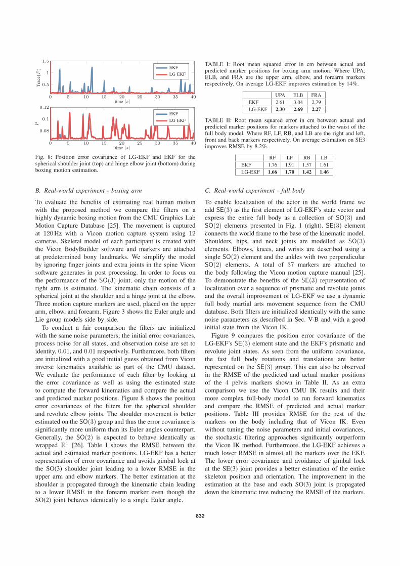
0 5 10 15 20 25 30 35 40
0.5
1
1.5
time [s]
Trac
e(P) EKF
LG EKF
0 5 10 15 20 25 30 35 40
0.08
0.1
0.12
time [s]
P
EKFLG EKF
Fig. 8: Position error covariance of LG-EKF and EKF for thespherical shoulder joint (top) and hinge elbow joint (bottom) duringboxing motion estimation.
B. Real-world experiment - boxing arm
To evaluate the benefits of estimating real human motionwith the proposed method we compare the filters on ahighly dynamic boxing motion from the CMU Graphics LabMotion Capture Database [25]. The movement is capturedat 120 Hz with a Vicon motion capture system using 12cameras. Skeletal model of each participant is created withthe Vicon BodyBuilder software and markers are attachedat predetermined bony landmarks. We simplify the modelby ignoring finger joints and extra joints in the spine Viconsoftware generates in post processing. In order to focus onthe performance of the SO(3) joint, only the motion of theright arm is estimated. The kinematic chain consists of aspherical joint at the shoulder and a hinge joint at the elbow.Three motion capture markers are used, placed on the upperarm, elbow, and forearm. Figure 3 shows the Euler angle andLie group models side by side.
To conduct a fair comparison the filters are initializedwith the same noise parameters; the initial error covariances,process noise for all states, and observation noise are set toidentity, 0.01, and 0.01 respectively. Furthermore, both filtersare initialized with a good initial guess obtained from Viconinverse kinematics available as part of the CMU dataset.We evaluate the performance of each filter by looking atthe error covariance as well as using the estimated stateto compute the forward kinematics and compare the actualand predicted marker positions. Figure 8 shows the positionerror covariances of the filters for the spherical shoulderand revolute elbow joints. The shoulder movement is betterestimated on the SO(3) group and thus the error covariance issignificantly more uniform than its Euler angles counterpart.Generally, the SO(2) is expected to behave identically aswrapped R1 [26]. Table I shows the RMSE between theactual and estimated marker positions. LG-EKF has a betterrepresentation of error covariance and avoids gimbal lock atthe SO(3) shoulder joint leading to a lower RMSE in theupper arm and elbow markers. The better estimation at theshoulder is propagated through the kinematic chain leadingto a lower RMSE in the forearm marker even though theSO(2) joint behaves identically to a single Euler angle.
TABLE I: Root mean squared error in cm between actual andpredicted marker positions for boxing arm motion. Where UPA,ELB, and FRA are the upper arm, elbow, and forearm markersrespectively. On average LG-EKF improves estimation by 14%.
UPA ELB FRAEKF 2.61 3.04 2.79LG-EKF 2.30 2.69 2.27
TABLE II: Root mean squared error in cm between actual andpredicted marker positions for markers attached to the waist of thefull body model. Where RF, LF, RB, and LB are the right and left,front and back markers respectively. On average estimation on SE3improves RMSE by 8.2%.
RF LF RB LBEKF 1.76 1.91 1.57 1.61LG-EKF 1.66 1.70 1.42 1.46
C. Real-world experiment - full body
To enable localization of the actor in the world frame weadd SE(3) as the first element of LG-EKF’s state vector andexpress the entire full body as a collection of SO(3) andSO(2) elements presented in Fig. 1 (right). SE(3) elementconnects the world frame to the base of the kinematic model.Shoulders, hips, and neck joints are modelled as SO(3)elements. Elbows, knees, and wrists are described using asingle SO(2) element and the ankles with two perpendicularSO(2) elements. A total of 37 markers are attached tothe body following the Vicon motion capture manual [25].To demonstrate the benefits of the SE(3) representation oflocalization over a sequence of prismatic and revolute jointsand the overall improvement of LG-EKF we use a dynamicfull body martial arts movement sequence from the CMUdatabase. Both filters are initialized identically with the samenoise parameters as described in Sec. V-B and with a goodinitial state from the Vicon IK.
Figure 9 compares the position error covariance of theLG-EKF’s SE(3) element state and the EKF’s prismatic andrevolute joint states. As seen from the uniform covariance,the fast full body rotations and translations are betterrepresented on the SE(3) group. This can also be observedin the RMSE of the predicted and actual marker positionsof the 4 pelvis markers shown in Table II. As an extracomparison we use the Vicon CMU IK results and theirmore complex full-body model to run forward kinematicsand compare the RMSE of predicted and actual markerpositions. Table III provides RMSE for the rest of themarkers on the body including that of Vicon IK. Evenwithout tuning the noise parameters and initial covariances,the stochastic filtering approaches significantly outperformthe Vicon IK method. Furthermore, the LG-EKF achieves amuch lower RMSE in almost all the markers over the EKF.The lower error covariance and avoidance of gimbal lockat the SE(3) joint provides a better estimation of the entireskeleton position and orientation. The improvement in theestimation at the base and each SO(3) joint is propagateddown the kinematic tree reducing the RMSE of the markers.
832

0 5 10 15 20 250
0.2
0.4
0.6
time [s]
Trac
e(P) EKF
LG EKF
Fig. 9: LG-EKF and EKF position error covariance of thetransformation of an SE(3) from world to base of the kinematicmodel. Since the transformation is an SE(3) element LG-EKF isable to accurately estimate it and its evolution over time. Prismaticjoints and Euler angles do not correctly represent SE(3) thus EKFcovariance increases during highly dynamic motion.
TABLE III: Root mean square error between predicted and actualmarker positions for full body motion capture. LG-EKF outperformsboth EKF and VICON IK for most of the markers. Refer to [25] formarker placement and naming details. Note, VICON IK prioritizesankle markers to avoid unrealistic sliding at the feet.
R Arm RSHO RELB RUPA RFRM RWRA RWRBVICON 6.33 4.57 5.17 4.64 7.01 6.91EKF 2.89 3.04 2.82 2.87 2.43 2.39LG-EKF 2.6 2.67 2.91 2.58 2.29 2.23
L Arm LSHO LELB LUPA LFRM LWRA LWRBVICON 7.82 5.96 6.32 8.19 11.11 10.74EKF 2.98 4.51 3.95 2.77 4.22 2.32LG-EKF 2.82 4.15 3.86 2.59 4.1 2.02
Torso and Head CLAV T10 STRN RFHD LFHD RBHD LBHDVICON 6.09 2.98 2.22 12.85 13.07 10.65 10.59EKF 1.74 1.55 1.72 1.3 1.18 1.5 1.49LG-EKF 1.64 1.45 1.59 1.26 1.13 1.45 1.43
R Leg RTHI RKNE RSHN RANK RHEE RTOE RMT5VICON 3.99 4.78 4.27 0.4 1.47 2.54 1.81EKF 2.06 2.42 2.34 1.15 1.18 0.94 1.06LG-EKF 1.93 2.4 2.33 1.14 1.16 0.93 1.04
L Leg LTHI LKNE LSHN LANK LHEE LTOE LMT5VICON 4.36 4.45 2.48 0.53 1.4 2.29 2.4EKF 2.09 2.01 1.35 1.06 1.22 1 1.18LG-EKF 2.07 1.98 1.34 1.04 1.21 1 1.16
VI. CONCLUSION
We proposed a novel algorithm for human motion estimationbased on body worn marker position measurements. Thehuman joints were described as Lie group members,including special orthogonal groups SO(2) and SO(3), anda special euclidean group SE(3). For stochastic inferenceon Lie groups the LG-EKF was employed, thus explicitlyaccounting for the non-euclidean geometry of the statespace. A constant acceleration motion model for humanmotion estimation on the group was developed and theJacobian of the marker position measurements was derived.The performance of the proposed method was evaluatedon both simulation and real-world motion capture data,comparing it with the Euler angles-based EKF as well asVicon IK for full body estimation. We showed that LG-EKFimproves estimation for highly dynamic motions and is notaffected by gimbal lock.
REFERENCES
[1] D. Kulic, G. Venture, K. Yamane, E. Demircan, I. Mizuuchi, andK. Mombaur, “Anthropomorphic Movement Analysis and Synthesis: A Survey of Methods and Applications,” IEEE Transactions onRobotics, vol. 32, no. 4, pp. 776–795, 2016.
[2] T. Sugihara, “Solvability-unconcerned inverse kinematics by thelevenberg–marquardt method,” IEEE Transactions on Robotics,vol. 27, no. 5, pp. 984–991, 2011.
[3] J. Steinbring, C. Mandery, N. Vahrenkamp, T. Asfour, and U. D.Hanebeck, “High-accuracy real-time whole-body human motiontracking based on constrained nonlinear kalman filtering,” arXivpreprint arXiv:1511.04278, 2015.
[4] A. Aristidou and J. Lasenby, “Real-time marker prediction and corestimation in optical motion capture,” The Visual Computer, vol. 29,no. 1, pp. 7–26, 2013.
[5] J. Steinbring, C. Mandery, F. Pfaff, F. Faion, T. Asfour, and U. D.Hanebeck, “Real-Time Whole-Body Human Motion Tracking Basedon Unlabeled Markers,” in IEEE Int. Conf. on Multisensor Fusion andIntegration for Intell. Systems (MFI). IEEE, 2016, pp. 607–614.
[6] V. Bonnet, G. Daune, V. Joukov, R. Dumas, P. Fraisse, D. Kulic,A. Seilles, S. Andary, and G. Venture, “A constrained extendedkalman filter for dynamically consistent inverse kinematics and inertialparameters identification,” in International Conference on BiomedicalRobotics and Biomechatronics (BioRob). IEEE, 2016, pp. 952–957.
[7] T. D. Barfoot and P. T. Furgale, “Associating Uncertainty WithThree-Dimensional Poses for Use in Estimation Problems,” IEEETransactions on Robotics, vol. 30, no. 3, pp. 679–693, jun 2014.
[8] M. Benallegue and F. Lamiraux, “Estimation and Stabilization ofHumanoid Flexibility Deformation Using Only Inertial MeasurementUnits and Contact Information,” International Journal of HumanoidRobotics, vol. 12, no. 3, p. 1550025, 2015.
[9] J. Cesic, I. Markovic, I. Cvisic, and I. Petrovic, “Radar and stereovision fusion for multitarget tracking on the special euclidean group,”Robotics and Autonomous Systems, vol. 83, pp. 338 – 348, 2016.
[10] G. Bourmaud, R. Megret, M. Arnaudon, and A. Giremus,“Continuous-Discrete Extended Kalman Filter on Matrix Lie GroupsUsing Concentrated Gaussian Distributions,” Journal of MathematicalImaging and Vision, vol. 51, no. 1, pp. 209–228, 2015.
[11] C. Hertzberg, R. Wagner, U. Frese, and L. Schroder, “IntegratingGeneric Sensor Fusion Algorithms with Sound State Representationsthrough Encapsulation of Manifolds,” Information Fusion, vol. 14,no. 1, pp. 57–77, jul 2013.
[12] Q. Rentmeesters, P. A. Absil, P. Van Dooren, K. Gallivan, andA. Srivastava, “An efficient particle filtering technique on thegrassmann manifold,” in IEEE International Conference on Acoustics,Speech and Signal Processing (ICASSP), 2010, pp. 3838–3841.
[13] J. Martinez-Del-Rincon, M. Lewandowski, J. C. Nebel, and D. Makris,“Generalized Laplacian eigenmaps for modeling and tracking humanmotions,” IEEE Trans. on Cyb., vol. 44, no. 9, pp. 1646–1660, 2014.
[14] M. Ding and G. Fan, “Multilayer Joint Gait-Pose Manifolds for HumanGait Motion Modeling,” IEEE Transactions on Cybernetics, vol. 45,no. 11, pp. 2413–2424, 2015.
[15] M. Devanne, H. Wannous, S. Berretti, P. Pala, M. Daoudi, andA. Del Bimbo, “3-D Human Action Recognition by Shape Analysisof Motion Trajectories on Riemannian Manifold,” IEEE Transactionson Cybernetics, vol. 45, no. 7, pp. 1340–1352, 2015.
[16] S. Brossette, A. Escande, G. Duchemin, B. Chretien, and A. Kheddar,“Humanoid posture generation on non-Euclidean manifolds,” IEEE-RAS Int. Conf. on Humanoid Robots, pp. 352–358, 2015.
[17] Y. Bar-Shalom, T. Kirubarajan, and X.-R. Li, Estimation withApplications to Tracking and Navigation. John Wiley & Sons, 2002.
[18] G. S. Chirikjian, Stochastic Models, Inform. Theory, and Lie Groups,Vol. 2: Analytic Methods and Modern Applications. Springer, 2012.
[19] J. M. Selig, “Lie Groups and Lie Algebras in Robotics,” in Comput.Noncommutative Algebra and Applications, 2005, pp. 101–125.
[20] W. Park, Y. Wang, and G. S. Chirikjian, “The Path-of-ProbabilityAlgorithm for Steering and Feedback Control of Flexible Needles,”Int. Journal of Robotics Research, vol. 29, no. 7, pp. 813–830, 2010.
[21] Y. Wang and G. S. Chirikjian, “Nonparametric Second-Order Theoryof Error Propagation on Motion Groups,” The International Journalof Robotics Research, vol. 27, no. 11, pp. 1258–1273, 2008.
[22] V. Joukov, R. D’Souza, and D. Kulic, “Human pose estimation fromimperfect sensor data via the extended kalman filter,” in InternationalSymposium on Experimental Robotics (ISER 2016). IEEE, 2016.
[23] D. Q. Huynh, “Metrics for 3d rotations: Comparison and analysis,” J.of Math. Imaging and Vision, vol. 35, no. 2, pp. 155–164, 2009.
[24] F. S. Grassia, “Practical parameterization of rotations using theexponential map,” J. of graphics tools, vol. 3, no. 3, pp. 29–48, 1998.
[25] F. De la Torre, J. Hodgins, A. Bargteil, X. Martin, J. Macey,A. Collado, and P. Beltran, “Guide to the carnegie mellon universitymultimodal activity (cmu-mmac) database,” Rob. Inst., p. 135, 2008.
[26] I. Markovic, J. Cesic, and I. Petrovic, “On wrapping the Kalman filterand estimating with the SO(2) group,” International Conference onInformation Fusion (FUSION), pp. 1–6, 2016.
833

92 publications
publication 5
V. Joukov, J. Ćesić, K. Westermann, I. Marković, D. Kulić and I. Petrović. Human motion
estimation on Lie groups using IMUmeasurements. IEEE/RSJ International Conference on
Intelligent Robots and Systems (IROS). Vancouver, Canada, 1965–1972, 2017.
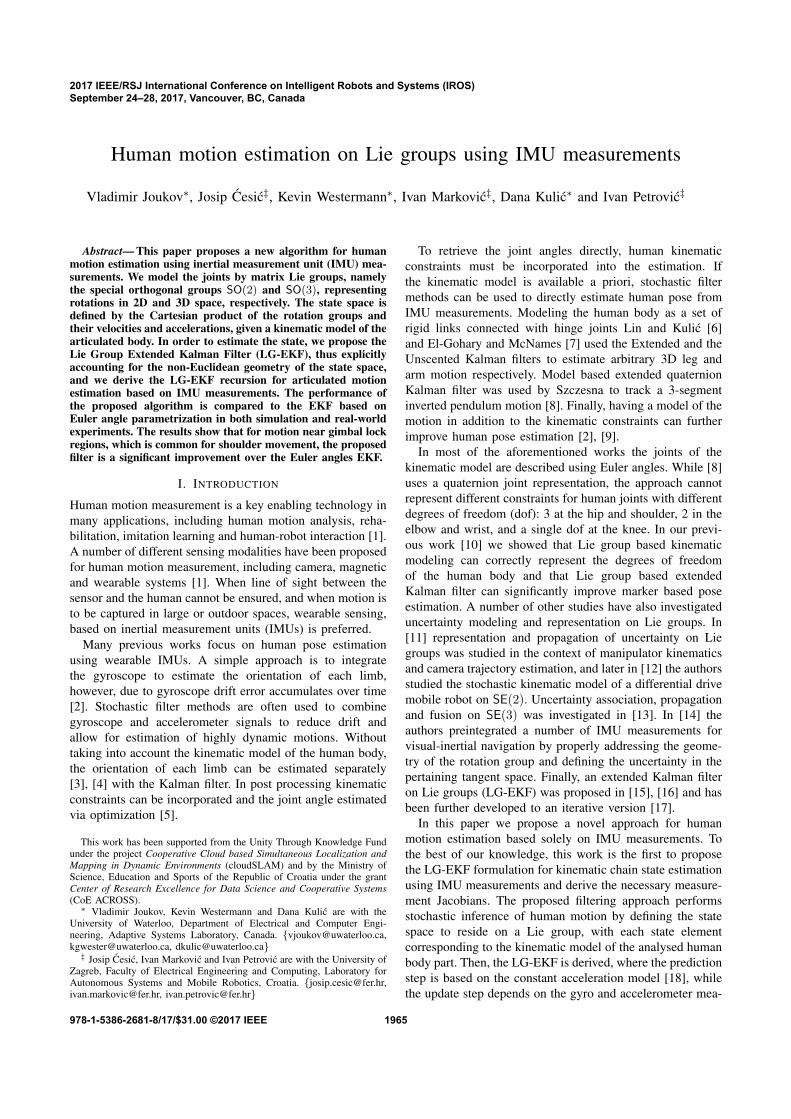
Human motion estimation on Lie groups using IMU measurements
Vladimir Joukov∗, Josip Cesic‡, Kevin Westermann∗, Ivan Markovic‡, Dana Kulic∗ and Ivan Petrovic‡
Abstract— This paper proposes a new algorithm for humanmotion estimation using inertial measurement unit (IMU) mea-surements. We model the joints by matrix Lie groups, namelythe special orthogonal groups SO(2) and SO(3), representingrotations in 2D and 3D space, respectively. The state space isdefined by the Cartesian product of the rotation groups andtheir velocities and accelerations, given a kinematic model of thearticulated body. In order to estimate the state, we propose theLie Group Extended Kalman Filter (LG-EKF), thus explicitlyaccounting for the non-Euclidean geometry of the state space,and we derive the LG-EKF recursion for articulated motionestimation based on IMU measurements. The performance ofthe proposed algorithm is compared to the EKF based onEuler angle parametrization in both simulation and real-worldexperiments. The results show that for motion near gimbal lockregions, which is common for shoulder movement, the proposedfilter is a significant improvement over the Euler angles EKF.
I. INTRODUCTION
Human motion measurement is a key enabling technology inmany applications, including human motion analysis, reha-bilitation, imitation learning and human-robot interaction [1].A number of different sensing modalities have been proposedfor human motion measurement, including camera, magneticand wearable systems [1]. When line of sight between thesensor and the human cannot be ensured, and when motion isto be captured in large or outdoor spaces, wearable sensing,based on inertial measurement units (IMUs) is preferred.
Many previous works focus on human pose estimationusing wearable IMUs. A simple approach is to integratethe gyroscope to estimate the orientation of each limb,however, due to gyroscope drift error accumulates over time[2]. Stochastic filter methods are often used to combinegyroscope and accelerometer signals to reduce drift andallow for estimation of highly dynamic motions. Withouttaking into account the kinematic model of the human body,the orientation of each limb can be estimated separately[3], [4] with the Kalman filter. In post processing kinematicconstraints can be incorporated and the joint angle estimatedvia optimization [5].
This work has been supported from the Unity Through Knowledge Fundunder the project Cooperative Cloud based Simultaneous Localization andMapping in Dynamic Environments (cloudSLAM) and by the Ministry ofScience, Education and Sports of the Republic of Croatia under the grantCenter of Research Excellence for Data Science and Cooperative Systems(CoE ACROSS).∗ Vladimir Joukov, Kevin Westermann and Dana Kulic are with the
University of Waterloo, Department of Electrical and Computer Engi-neering, Adaptive Systems Laboratory, Canada. [email protected],[email protected], [email protected]‡ Josip Cesic, Ivan Markovic and Ivan Petrovic are with the University of
Zagreb, Faculty of Electrical Engineering and Computing, Laboratory forAutonomous Systems and Mobile Robotics, Croatia. [email protected],[email protected], [email protected]
To retrieve the joint angles directly, human kinematicconstraints must be incorporated into the estimation. Ifthe kinematic model is available a priori, stochastic filtermethods can be used to directly estimate human pose fromIMU measurements. Modeling the human body as a set ofrigid links connected with hinge joints Lin and Kulic [6]and El-Gohary and McNames [7] used the Extended and theUnscented Kalman filters to estimate arbitrary 3D leg andarm motion respectively. Model based extended quaternionKalman filter was used by Szczesna to track a 3-segmentinverted pendulum motion [8]. Finally, having a model of themotion in addition to the kinematic constraints can furtherimprove human pose estimation [2], [9].
In most of the aforementioned works the joints of thekinematic model are described using Euler angles. While [8]uses a quaternion joint representation, the approach cannotrepresent different constraints for human joints with differentdegrees of freedom (dof): 3 at the hip and shoulder, 2 in theelbow and wrist, and a single dof at the knee. In our previ-ous work [10] we showed that Lie group based kinematicmodeling can correctly represent the degrees of freedomof the human body and that Lie group based extendedKalman filter can significantly improve marker based poseestimation. A number of other studies have also investigateduncertainty modeling and representation on Lie groups. In[11] representation and propagation of uncertainty on Liegroups was studied in the context of manipulator kinematicsand camera trajectory estimation, and later in [12] the authorsstudied the stochastic kinematic model of a differential drivemobile robot on SE(2). Uncertainty association, propagationand fusion on SE(3) was investigated in [13]. In [14] theauthors preintegrated a number of IMU measurements forvisual-inertial navigation by properly addressing the geome-try of the rotation group and defining the uncertainty in thepertaining tangent space. Finally, an extended Kalman filteron Lie groups (LG-EKF) was proposed in [15], [16] and hasbeen further developed to an iterative version [17].
In this paper we propose a novel approach for humanmotion estimation based solely on IMU measurements. Tothe best of our knowledge, this work is the first to proposethe LG-EKF formulation for kinematic chain state estimationusing IMU measurements and derive the necessary measure-ment Jacobians. The proposed filtering approach performsstochastic inference of human motion by defining the statespace to reside on a Lie group, with each state elementcorresponding to the kinematic model of the analysed humanbody part. Then, the LG-EKF is derived, where the predictionstep is based on the constant acceleration model [18], whilethe update step depends on the gyro and accelerometer mea-
2017 IEEE/RSJ International Conference on Intelligent Robots and Systems (IROS)September 24–28, 2017, Vancouver, BC, Canada
978-1-5386-2681-8/17/$31.00 ©2017 IEEE 1965

Fig. 1. Left: 3D Arm model showing simulation IMU placement. Middle:Lie group-based arm model with attached IMU units for dynamic motionsimulation. Right: Euler angle-based arm model.
surements of the IMU units. We compare the performanceof the proposed algorithm with an EKF based on the Eulerangles parametrization both in simulation and real-worldexperiments. The results show that the proposed approachsignificantly improves performance and is not affected bygimbal lock.
The rest of the paper is organised as follows. In Section IIwe present the mathematical fundamentals addressing Liegroups and associated uncertainties. In Section III we presentthe novel LG-EKF, while in Section IV we briefly describethe EKF based on Euler angles. Section V presents thevalidation results and Section VI concludes the paper.
II. MATHEMATICAL BACKGROUND
In this section we provide the mathematical background forhuman motion estimation on matrix Lie groups, based on thehuman body modeling approach and the corresponding statespace construction first proposed in [19].
A. Construction of the state space
We construct the state space by using Lie group represen-tatives for each joint of interest. As an example we considerthe model of a human arm illustrated in Fig. 1. An exampleof group G representing the state space for this model is
G =
shoulder︷ ︸︸ ︷SO(3)×
elbow︷ ︸︸ ︷SO(2)× SO(2) . (1)
The first element in (1) describes the shoulder employing aspecial orthogonal group SO(3) and providing 3 DoF mobil-ity, while the second and third elements jointly model the 2DoF motion of the flexion/extension and internal rotation ofthe elbow joint, where each element of a special orthogonalgroup SO(2) contributes a single DoF. Note that the choiceof the state space only incorporates system variables and notthe kinematic model geometry.
B. Lie groups and Lie algebra
A Lie group G is a group which also has the structure ofa smooth manifold. The group operators, composition andinversion, are smooth operations. Each point X ∈ G hasan associated tangent space TX(G) [20]. This linear tangentspace is usually placed at the group identity, and is called theLie algebra of G, which we denote by g [21]. The Lie algebra
g, which is of the same dimension as G, admits a binaryoperation [·, ·] called the Lie bracket, which reflects the non-commutative content of the group operation. Furthermore, ifthe group G is a matrix Lie group, then G ⊂ Rn×n and groupoperations are simply matrix multiplication and inversion.
The Lie algebra g ⊂ Rn×n associated to a p-dimensionalmatrix Lie group G ⊂ Rn×n is a p-dimensional vectorspace defined by a basis consisting of p real matricesEr, r = 1, . . . , p, often referred to as generators [22]. Inparticular, a Lie algebra is an open neighbourhood around0p in the tangent space of G at the identity In. The matrixexponential expG and matrix logarithm logG establish a localdiffeomorphism between G and g as
expG : g→ G and logG : G→ g. (2)
Furthermore, a natural relation exists between the p-dimensional Lie algebra g and the Euclidean space Rp, andis given through a linear isomorphism
[·]∨G : g→ Rp and [·]∧G : Rp → g. (3)
For brevity, we will use the following notation [17]
exp∧G(x) = expG([x]∧G) and log∨G(X) = [logG(X)]∨G , (4)
where x ∈ Rp and X ∈ G.Since Lie groups are generally non-commutative, i.e.,
XY 6= Y X , we also need to employ the adjoint representa-tions. The adjoint representation of G on g, AdG, can be seenas as a way of representing the elements of the group as alinear transformation of the group’s algebra, and in general,it measures the failure of X ∈ G to commute with elementsof G near the identity [23]. The adjoint representation of g,adG, is in fact the differential of AdG at the identity element.For a commutative group, the map ad evaluates to zero.
C. Concentrated Gaussian distribution
To make use of EKF on Lie groups, we need to establishfirst a notion of a Gaussian distribution on Lie groups. Adistribution on a Lie group that is tightly focused, meaningthat almost all the mass of the distribution is concentratedin a small neighborhood around the mean, can be expressedin the Lie algebra [13], [24], and this concept is called aconcentrated Gaussian distribution.
Let X ∈ G be a random variable following a concentratedGaussian distribution with mean µ and covariance P as
X = µ exp∧G(ε), X ∼ G(µ, P ), (5)
where ε ∼ NRp(0p, P ) is a zero-mean Gaussian distributionwith covariance P ⊂ Rp×p defined in the Lie algebra, i.e.,the Euclidean space Rp. We can see form (5) that the meanvalue µ is defined on G, while the associated uncertaintyresides in Rp. Roughly, this concept allows us to work withthe covariance directly in Rp and use Euclidean tools, almostas we would with a ‘classical’ Gaussian distribution [16].
1966

D. Special orthogonal groups SO(2) and SO(3)
The special orthogonal group SO(n) is the matrix group
SO(n) =X ⊂ Rn×n |XTX = I, det(X) = 1
. (6)
For n = 2, 3 this group defines rotations in 2D and 3D,respectively. The algebra so(n) comprises of n × n skew-symmetric matrices. For Euclidean vectors x = φ and x =[φ1 φ2 φ3]T, the algebras so(2) and so(3) amount to
x∧SO(2) =
[0 −φφ 0
], x∧SO(3) =
0 −φ3 φ2φ3 0 −φ1−φ2 φ1 0
, (7)
where (·)∧SO(n) : Rn → so(n), while its inverse, (·)∨SO(n) :so(n)→ Rn, follows trivially from (7).
For SO(2), the exponential map yields the classical 2Drotation matrix, while the logarithm evaluates to simple ex-traction of φ into a skew-symmetric matrix form in (7). SinceSO(2) is commutative, its adjoint representations are trivial:AdSO(2) is a unit map and adSO(2) is zero. The exponentialfor SO(3), performing mapping expSO(3) : so(3) → SO(3),is given as
exp∧SO(3)(x) = cos(|x|)I3+
+ (1− cos(|x|))xxT
|x|2+ sin(|x|)
x∧SO(3)
|x|.
(8)
The logarithm, performing mapping logSO(3) : SO(3) →so(3), is given as
logSO(3)(X) =θ
2 sin(θ)(X −XT)
s.t. 1 + 2 cos(θ) = Tr(X)θ 6= 0 −π < θ < π
θ = 0 log(X) = 0.
(9)
The adjoints AdSO(3) and adSO(3) are respectively given as
AdSO(3)(X) = X and adSO(3)(x) = x∧SO(3) . (10)
In the sequel we present the new human motion estimationmethod based on the LG-EKF using IMU measurements.
III. HUMAN MOTION ESTIMATION ON LIE GROUPS
Our goal is to estimate the pose of a kinematic chainrepresented via Lie groups (as described in section II-A),as well as its velocity and acceleration, using measurementsfrom rigidly attached inertial measurement units at each link.To utilize LG-EKF for such state estimation, assuming aconstant acceleration model (CA) [25] for each joint, wederive the necessary gyroscope and accelerometer measure-ment models and their Jacobians.
A. Motion prediction step
We assume that the motion model of the system can bedescribed with the following equation [16]
Xk+1 = f(Xk, nk) = Xk exp∧G(
Ωk + nk
), (11)
where Xk ∈ G is the state of the system at time k, G isa p-dimensional Lie group, nk ∼ NRp(0p×1, Qk) is zeromean white Gaussian noise with covariance Qk, and Ωk =Ω(Xk) : G→ Rp is a non-linear C2 function.
In our approach, similar to our previous work [19], weassume the human motion to follow a constant accelerationmodel and our state space G is then constructed to includethe positional, velocity and acceleration components block-diagonally. Hence exponentials and logarithms will keep thestate in the block diagonal arrangement as well. The motionmodel of a single joint i is given as
Ωik =
Tωik + T2
2 αik
Tαik0
∈ R3di , nk =
T2
2 nik
Tniknik
∈ R3di
(12)
where ωik and αik are the angular velocity and angularacceleration represented in the Lie algebra1. The term nikrepresents the acceleration increment during the k-th sam-pling period [25], di represents the number of DoFs of thei-th joint, and T is the sampling period.
Assuming that the posterior distribution at step k fol-lows the concentrated Gaussian distribution G(µk, Pk), andfollowing the LG-EKF prediction step [19], the resultingprediction can be approximated with a concentrated Gaussiandistribution G(µk+1|k, Pk+1|k). The mean propagation of theLG-EKF is:
µk+1|k = µk exp∧G(
Ωk
), (13)
while the covariance prediction is computed as
Pk+1|k = FkPkFTk + ΦG(Ωk)QkΦG(Ωk)T . (14)
The operator Fk can be seen as a matrix Lie group equivalentto the Jacobian of f(Xk, nk), and is calculated by
Fk = AdG(
exp∧G(−Ωk
))+ ΦG(Ωk)Lk
Lk =∂
∂εΩ (µk exp∧G (ε))|ε=0 .
(15)
The term Lk represents the linearisation term where theargument of the motion model is the mean of the currentstate Xk with an incremental perturbation additively added ineach of the p directions. Contrary to the conventional EKF, alinear additive process noise affects the system as a functionof the current state of the system over the transformationΦG(Ωk)QkΦG(Ωk)T, where ΦG appears due to the displace-ment of the tangential space during the prediction step, andis given by:
ΦG(v) =∞∑i=0
(−1)i
(i+ 1)!adG(v)i , v ∈ Rp . (16)
1Euclidean space Rp, p ∈ N is a matrix Lie group and in order toconstruct G we employ its matrix representation obtained by simple matrixembedding. The matrix representation of the Euclidean space is also asubgroup of SE(n) where a pure translation is employed [26].
1967

B. Measurement update step
We next derive the update step by employing gyro andaccelerometer measurements of IMUs attached to a humanbody. The discrete measurement model on the matrix Liegroup is modelled as:
Zk+1 = h(Xk+1) exp∧G′ (mk+1) , (17)
where Zk+1 ∈ G′, h : G → G′ is a C1 function, G′ is ap′-dimensional Lie group and mk+1 ∼ NRq (0q×1, Rk+1)is zero-mean white Gaussian noise with covariance Rk+1.The update step of the filter strongly resembles the standardEKF update procedure, relying on the Kalman gain Kk+1
and innovation vector νk+1 calculated as:
Kk+1 = Pk+1|kHTk+1
(Hk+1Pk+1|kHT
k+1 +Rk+1
)−1νk+1 = Kk+1 log∨G′
(h(µk+1|k)−1Zk+1
). (18)
The matrix Hk+1 can be seen as the matrix Lie groupequivalent of the Jacobian of h(Xk+1), and is given as:
Hk+1 =∂
∂εlog∨G′
(h(µk+1|k)−1h(µεk+1|k)
)|ε=0
,
where h(µεk+1|k) = h(µk+1|k exp∧G (ε)), describes the varia-tion of measurements for an infinitesimal motion ε. We nowevaluate the matrix Hk+1 based on gyro and accelerometermeasurements.
C. Gyro update
The measurement function of the gyro measurement is:
h(Xk+1|k) =n∑i=1
Ks,Ri ωik+1|k , (19)
where n is the number of joints preceding the gyro sensor s.The term Ks,Ri = Ks,Ri (Xk+1|k) is the rotational componentof the forward kinematics between the i-th joint and thegyro sensor s, thus affecting its measurement [27]. The gyromeasurements are affected by position (through kinematics)and velocity, hence the corresponding parts of Hk+1 matrixneed to be evaluated.
By applying partial derivatives and evaluating the multi-variate limits similarly to [28], the part of Hk+1 relating thegyro measurement to the orientation of the l-th joint Hθ,lk+1
is:
Hθ,l,rk+1 =l−1∑i=1
Ks,Rl El,rT
θl−1
k+1|kKl,Ri ωik+1|k , (20)
where Ki,Rl represents the rotation between the i-th and l-th joint, θlk+1|k is the position of the l-th joint, while El,r
represents the r-th generator of a Lie group representingthe l-th joint [24]. Each of the generators represents aninfinitesimal motion in one of the directions of a Lie group.
The part of Hk+1 relating the gyro measurement to thevelocity of the l-th joint Hω,lk+1 is given as:
Hω,lk+1 = Ks,Rl . (21)
Since gyro measurement (19) is not a function of the jointaccelerations, the part of the Hk+1 matrix relating gyro
measurements to l-th joint acceleration components is filledwith zero values; Hα,lk+1 = 0.
D. Accelerometer update
The measurement function corresponding to the accelerom-eter measurement is:
h(Xk+1|k) =
point acceleration︷ ︸︸ ︷Ks,R0 pk+1|k +
gravity component︷ ︸︸ ︷Ks,R0 g , (22)
where the first term emerges due to dynamics of a body,while the second term arises due to gravity. The superscriptR denotes that only the rotation part is embedded into anSE(3) member, while the translation part is set to 0. The termpk+1|k represents an acceleration of the sensor s representedin the base frame and given in homogeneous coordinates,while g is the gravity vector in homogeneous coordinates.In order to evaluate pk+1|k, we start from defining the IMUposition as:
pk+1|k = K0sO (23)
where O = [0 0 0 1]T is the origin represented in homoge-neous coordinates. The forward kinematics are:
K0s = T 0
1 θ1k+1|kT
12 θ
2k+1|k · · ·T
n−1n θnk+1|k (24)
Each part of the forward kinematics Ki−1i = T i−1i θik+1|kconsists of the constant transformation T i−1i and the positionof the i-th joint θik+1|k. In order to sequentially apply amatrix multiplication inducing each joint state, we describejoints as 4 × 4 transformation matrices (in terms of Liegroups denoted as special euclidean group SE(3)). We nowevaluate the first two derivatives of sensor position pk+1|k.The velocity of the point pk+1|k evaluates to:
pk+1|k =n∑i=1
(K0iS
i,ωk+1|kK
is
)O , (25)
where the summation iterates over n joints affecting sensors, while the term Si,ωk+1|k is given as:
Si,ωk+1|k =
di∑r=1
(ωi,rk+1|kE
i,r), (26)
which is a function of the number of degrees of freedomdi of the i-th joint, and the superscript ω denotes that thevelocity components are summed up. The acceleration of thepoint pk+1|k evaluates to:
pk+1|k =
centripetal force component I︷ ︸︸ ︷n∑i=1
( i∑j=1
(K0jS
j,ωk+1|kK
ji
)Si,ωk+1|kK
is
)O+ (27)
centripetal force component II︷ ︸︸ ︷n∑i=1
(K0iS
i,ωk+1|k
n∑j=i+1
(KijS
j,ωk+1|kK
js
))O+
n∑i=1
(K0iS
i,αk+1|kK
is
)O︸ ︷︷ ︸
joint acceleration component
.
1968

The acceleration pk+1|k consists of two components – thecentripetal force component and joint acceleration compo-nent, which we emphasize in (27).
We now proceed to linearize and evaluate the part ofHk+1
corresponding to the accelerometer measurement and joint l:[Hlk+1
1
]=
∂Ks,R0
∂X lk+1|k
(pk+1|k + g
)+Ks,R0
∂pk+1|k∂X l
k+1|k. (28)
In order to evaluate (28) we compute partial derivativesof Ks,R0 and pk+1|k with respect to position, velocity, andacceleration of X l
k+1|k. The detailed derivation is providedin the supplementary material [29].
Finally, having evaluated Hk+1, the measurement updatestep is calculated as [16]:
µk+1 = µk+1|k exp∧G (νk+1) (29)
Pk+1 = ΦG(νk+1) (I −Kk+1Hk+1)Pk+1|kΦG(νk+1)T .
IV. EULER ANGLE BASED APPROACH
The proposed approach is compared to a conventional EKFapplied to a standard kinematic model defined with revoluteand prismatic joints [30]. Three perpendicular revolute joints(Euler angles) can be used to model human spherical jointssuch as the shoulder and the hip. The state of the EKF isdefined as the position q, velocity q, and acceleration q ofthe joints. Just as in the LG-EKF formulation we assumeconstant acceleration of each joint.
It is also possible to model the kinematics using quater-nions to represent the joint state. Since rotations are repre-sented by unit quaternions, one approach when using EKFis to normalize the state estimate after each iteration [8].This normalization, while correctly propagating the errorcovariance, no longer optimally performs the state updatestep [31]. Similar to rotation matrices quaternions have atangent space and thus, it is possible to apply LG-EKF to aquaternion based state representation using the SU(2) group,in this case we expect similar results to our formulation.
V. VALIDATION RESULTS
We validate the proposed approach both in simulation andwith real human motion. First, in simulation, we demonstratethe benefits of LG-EKF over EKF when using IMU measure-ments during highly dynamical movements whose motion isbetter described on the group and show that unlike EKF, LG-EKF is not affected by gimbal lock. Next, we evaluate theperformance of LG-EKF and EKF on real IMU data of adynamic figure eight arm movement sequence.
A. Simulation Validation
1) Dynamic Motion: To test the properties of LG-EKF,we simulate a human shown in Fig. 1, modeled with (1).Two IMUs are attached to the humerus and radius at offsetsof [0.1 0.1 0.3]T, and [0.1 0.1 0.4]T respectively.
It is possible to generate Brownian motion either on thegroup or on Euler angles to exactly match the constantacceleration with zero mean Gaussian noise assumption ofLG-EKF or EKF. Since large constant acceleration in one
0 1 2 3 4 5
−4
−2
0
2
4
time [s]
Acc
eler
atio
n[r
ad/s
]
Acceleration of SO(3) × SO(2) × SO(2)
α11
α21
α31
α2
α3
0 1 2 3 4 50
0.2
0.4
0.6
0.8
time [s]
Pos.
RM
SE[m
]
Position RMSE of Wrist IMU
EKFLG-EKF
Fig. 2. Performance of EKF and LG-EKF based on Brownian motionon Lie Algebra. Since LG-EKF has an accurate motion model it correctlytracks the arm movement. Once the angular accelerations on the Lie Algebrabecome large, the constant Euler angle acceleration model of EKF doesnot provide a good state prediction and EKF cannot maintain an accurateestimate. α1 denotes SO(3) with 3 dofs, while α2 and α3 correspond toSO(2) joints with a single dof.
representation implies a quickly changing acceleration in theother, we can expect the filter with the correct motion modelto significantly outperform the other in high accelerationregions. Figure 2 shows the Brownian motion generatedon the group representation of the arm and the root meansquared error (RMSE) in position estimation of the wristIMU for EKF and LG-EKF. It is clear that during highconstant accelerations on the group, Euler angle based EKFcannot accurately track the motion.
However, it is unlikely that human motion will satisfy theconstant acceleration assumption. Thus, in order to compareEKF and LG-EKF without being biased to a specific motionrepresentation we generate a dynamic trajectory in task spaceand utilize inverse kinematics to recover joint angles of theEuler angle model. Next we numerically differentiate thetrajectory to retrieve joint velocities and accelerations andgenerate the IMU measurements using forward kinematics.The task space trajectory is created by cubic splining ofpoints in the reachable workspace generated from a univari-ate distribution. This setup creates a highly dynamic motionas can be seen from the positions of the two IMUs shown inFig. 3. Simulated IMUs are sampled at 100 Hz and zero meanGaussian noise with standard deviations of 0.01 rad
s and 0.1ms2
is added to the gyroscope and accelerometer measurementsrespectively. For both filters the initial covariances were setto a diagonal matrix of a 10−3 denoting accurate knowledgeof the initial state. For the process noise, for each triplet[φ ω α] or [q q q], noise of standard deviation η is injectedinto α and is propagated to ω and φ by integration. Thus,for each triplet the process noise covariance is GGT whereG = [T
2
2 T 1]η. For the dynamic motion simulation η wasset to 10 rad
s2 per iteration. The observation noise was set tothe true sensor noise values.
To compare the estimate with the ground truth, we use
1969

−0.50
0.5 −0.5
00.5
0
1
x [m]
y[m
]
z[m
]
RadialHumerus
Fig. 3. 10 Second simulation trajectory of the IMUs attached to thehumerus and radial undergoing the generated highly dynamic motion.
0 2 4 6 8 100
2
4
6
8
·10−2
time [s]
DF
Shoulder RMSE. LG-EKFRMSE = 0.011, EKFRMSE = 0.037
LG-EKFEKF
0 2 4 6 8 100
1
2·10−2
time [s]
DF
Elbow RMSE. LG-EKFRMSE = 0.005, EKFRMSE = 0.005
LG-EKFEKF
Fig. 4. Error between the actual and estimated rotations at the shoulderand elbow joint for LG-EKF and EKF during task space generated dynamicmotion. Estimation of shoulder rotation is significantly improved using theSO(3) model.
the deviation from the identity matrix as the distance metric[32]:
DF =∥∥I −RT
eRgt∥∥F
(30)
where Re and Rgt are the estimated and ground truth rotationmatrices of each joint and ‖·‖F denotes the Frobenius norm.
Figure 4 shows the comparison between the LG-EKF andEKF using this distance metric for the shoulder and elbowjoints. The LG-EKF significantly outperforms the EKF filter,which is due to LG-EKF’s ability to handle gimbal lock asexplained in the next section.
2) Gimbal Lock: Next we investigate the impact of gimballock on the proposed approach. Any set of Euler angles willlose a degree of freedom when two of the rotation axesalign [33], implying that in that configuration the rotationabout the locked axis cannot be correctly estimated by EKF.Typically the order of the joint axes is carefully selected totry and avoid the lock, however in human motion estimation,gimbal lock often takes place at the shoulder joint due to itshigh manoeuvrability. Unlike the Euler angle formulation, an
Fig. 5. Simulation model used for gimbal lock validation.
0 0.2 0.4 0.6 0.8 1 1.2 1.4 1.6 1.8 20.00
0.02
0.04
0.06
0.08
0.10
0.12
time [s]
DF
LG-EKFEKF
Fig. 6. LG-EKF and EKF estimation during gimbal lock. Both filtersaccurately estimate the rotation about the y axis until the system gets closeto the gimbal lock, which happens at 1 second. After the rotation about y theEuler angle model is in gimbal lock and thus EKF cannot accurately trackthe orientation until the lock is escaped at 1.5 seconds. Once Euler anglesescape the gimbal lock, EKF can regain an accurate estimate of the roll andpitch orientation using the accelerometer’s gravity measurement. However,any error in yaw during gimbal lock accumulates. LG-EKF estimation isunaffected by gimbal lock.
SO(3) representation of the spherical joint does not sufferfrom gimbal lock and thus LG-EKF will accurately estimateany rotation.
To demonstrate the benefits of LG-EKF over EKF duringgimbal lock we simulate a single spherical joint at theorigin with a single IMU attached at an offset of 0.1meters in x. The simulated model is shown in Fig. 5. Aquintic polynomial is used to generate a smooth trajectory,sampling at 100 Hz. First, the model experiences a 1 secondrotation about the world y axis with initial position 0 rad andfinal positions π
2 rad and zero initial and final velocity andacceleration. In the Euler angle model this motion aligns thefirst and third revolute joint axes putting it into a singularityand removing a degree of freedom (gimbal lock). Next, themodel experiences the same 1 s rotation in the now lockedworld z axis. In order to focus only on the gimbal lockproblem, no noise was added to the IMU measurements.Measurement noise, process noise, and initial covarianceswere set as described in Sec. V-A.1. Figure 6 shows thedistance metric described in (30).
When Euler angles enter gimbal lock, the Euler anglebased Jacobian is singular and thus the linearized systemis no longer observable. In this case EKF cannot accuratelyestimate the states. By plotting the condition number of theobservability matrixOb = [Hk HkFk · · · ]T of the linearizedsystem we can visualize the ability of the filters to handlegimbal lock (Fig. 7).
Furthermore we show that the Lie group motion modelis superior for process noise representation over the Eulerangle motion model. Consider a single SO(3) joint with anIMU attached at some offset. Independent of the initial SO(3)state, addition of zero mean, Gaussian process noise to thestate results in a consistent distribution of the end effector
1970
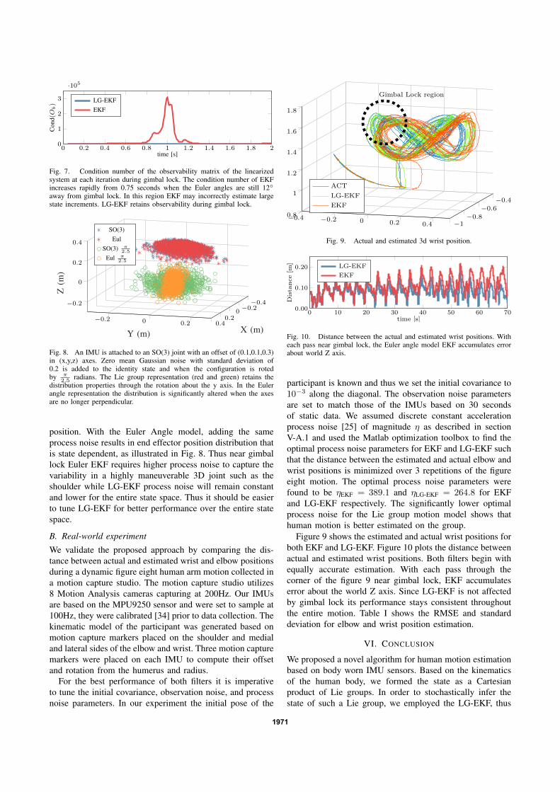
0 0.2 0.4 0.6 0.8 1 1.2 1.4 1.6 1.8 20
1
2
3
·105
time [s]
Con
d(O
b)
LG-EKFEKF
Fig. 7. Condition number of the observability matrix of the linearizedsystem at each iteration during gimbal lock. The condition number of EKFincreases rapidly from 0.75 seconds when the Euler angles are still 12away from gimbal lock. In this region EKF may incorrectly estimate largestate increments. LG-EKF retains observability during gimbal lock.
−0.4−0.2
00.2
0.4−0.2 0 0.2
−0.2
0
0.2
0.4
X (m)Y (m)
Z(m
)
SO(3)Eul
SO(3) π2.5
Eul π2.5
Fig. 8. An IMU is attached to an SO(3) joint with an offset of (0.1,0.1,0.3)in (x,y,z) axes. Zero mean Gaussian noise with standard deviation of0.2 is added to the identity state and when the configuration is rotedby π
2.5radians. The Lie group representation (red and green) retains the
distribution properties through the rotation about the y axis. In the Eulerangle representation the distribution is significantly altered when the axesare no longer perpendicular.
position. With the Euler Angle model, adding the sameprocess noise results in end effector position distribution thatis state dependent, as illustrated in Fig. 8. Thus near gimballock Euler EKF requires higher process noise to capture thevariability in a highly maneuverable 3D joint such as theshoulder while LG-EKF process noise will remain constantand lower for the entire state space. Thus it should be easierto tune LG-EKF for better performance over the entire statespace.
B. Real-world experiment
We validate the proposed approach by comparing the dis-tance between actual and estimated wrist and elbow positionsduring a dynamic figure eight human arm motion collected ina motion capture studio. The motion capture studio utilizes8 Motion Analysis cameras capturing at 200Hz. Our IMUsare based on the MPU9250 sensor and were set to sample at100Hz, they were calibrated [34] prior to data collection. Thekinematic model of the participant was generated based onmotion capture markers placed on the shoulder and medialand lateral sides of the elbow and wrist. Three motion capturemarkers were placed on each IMU to compute their offsetand rotation from the humerus and radius.
For the best performance of both filters it is imperativeto tune the initial covariance, observation noise, and processnoise parameters. In our experiment the initial pose of the
−0.4 −0.2 0 0.2 0.4 −1−0.8
−0.6
−0.4
0.8
1
1.2
1.4
1.6
1.8
Gimbal Lock region
ACTLG-EKFEKF
Fig. 9. Actual and estimated 3d wrist position.
0 10 20 30 40 50 60 700.00
0.10
0.20
time [s]
Dis
tanc
e[m
] LG-EKFEKF
Fig. 10. Distance between the actual and estimated wrist positions. Witheach pass near gimbal lock, the Euler angle model EKF accumulates errorabout world Z axis.
participant is known and thus we set the initial covariance to10−3 along the diagonal. The observation noise parametersare set to match those of the IMUs based on 30 secondsof static data. We assumed discrete constant accelerationprocess noise [25] of magnitude η as described in sectionV-A.1 and used the Matlab optimization toolbox to find theoptimal process noise parameters for EKF and LG-EKF suchthat the distance between the estimated and actual elbow andwrist positions is minimized over 3 repetitions of the figureeight motion. The optimal process noise parameters werefound to be ηEKF = 389.1 and ηLG-EKF = 264.8 for EKFand LG-EKF respectively. The significantly lower optimalprocess noise for the Lie group motion model shows thathuman motion is better estimated on the group.
Figure 9 shows the estimated and actual wrist positions forboth EKF and LG-EKF. Figure 10 plots the distance betweenactual and estimated wrist positions. Both filters begin withequally accurate estimation. With each pass through thecorner of the figure 9 near gimbal lock, EKF accumulateserror about the world Z axis. Since LG-EKF is not affectedby gimbal lock its performance stays consistent throughoutthe entire motion. Table I shows the RMSE and standarddeviation for elbow and wrist position estimation.
VI. CONCLUSION
We proposed a novel algorithm for human motion estimationbased on body worn IMU sensors. Based on the kinematicsof the human body, we formed the state as a Cartesianproduct of Lie groups. In order to stochastically infer thestate of such a Lie group, we employed the LG-EKF, thus
1971

TABLE IROOT MEAN SQUARED ERROR OF ESTIMATED AND ACTUAL ELBOW AND
WRIST POSITIONS FOR THE TWO FILTERS. THE PROPOSED LG-EKFIMPROVES THE POSITION ESTIMATE BY 30% OVER EKF.
Elbow RMSE [cm] Wrist RMSE [cm]LG-EKF 5.2 ± 2.6 6.9 ± 2.7
EKF 7.4 ± 3.6 9.9 ± 3.8
explicitly accounting for the non-Euclidean geometry of thestate space. A constant acceleration motion model on thegroup was developed for the LG-EKF prediction step andthe Jacobian of the IMU (gyroscope and accelerometer mea-surements), was derived for the update step. The performanceof the proposed method was evaluated in both simulation andreal-world data, comparing it with the EKF based on Eulerangles. The proposed algorithm can estimate human motionwith lower end effector position RMSE than the EKF andis not affected by gimbal lock. Future work will includefull body pose estimation based on wearable IMU sensorsand investigating using SE(3) joint types that can representtransformation matrices to accommodate for translations in3D space and handle the free flyer problem.
REFERENCES
[1] D. Kulic, G. Venture, K. Yamane, E. Demircan, I. Mizuuchi, andK. Mombaur, “Anthropomorphic movement analysis and synthesis: Asurvey of methods and applications,” IEEE Transactions on Robotics,vol. 32, no. 4, pp. 776–795, 2016.
[2] V. Bonnet, C. Mazza, J. McCamley, and A. Cappozzo, “Use ofweighted fourier linear combiner filters to estimate lower trunk 3dorientation from gyroscope sensors data,” Journal of neuroengineeringand rehabilitation, vol. 10, no. 1, p. 29, 2013.
[3] X. Yun and E. R. Bachmann, “Design, implementation, and exper-imental results of a quaternion-based kalman filter for human bodymotion tracking,” IEEE transactions on Robotics, vol. 22, no. 6, pp.1216–1227, 2006.
[4] G. Ligorio and A. M. Sabatini, “A novel kalman filter for humanmotion tracking with an inertial-based dynamic inclinometer,” IEEETransactions on Biomedical Engineering, vol. 62, no. 8, pp. 2033–2043, 2015.
[5] H. Zhou, T. Stone, H. Hu, and N. Harris, “Use of multiple wearableinertial sensors in upper limb motion tracking,” Medical engineering& physics, vol. 30, no. 1, pp. 123–133, 2008.
[6] J. F. Lin and D. Kulic, “Human pose recovery using wireless inertialmeasurement units,” Physiological measurement, no. 12, p. 2099,2012.
[7] M. El-Gohary and J. McNames, “Shoulder and elbow joint angle track-ing with inertial sensors,” Biomedical Engineering, IEEE Transactionson, vol. 59, no. 9, pp. 2635–2641, 2012.
[8] A. Szczesna and P. Pruszowski, “Model-based extended quaternionkalman filter to inertial orientation tracking of arbitrary kinematicchains,” SpringerPlus, vol. 5, no. 1, p. 1965, 2016.
[9] V. Joukov, B. Vincent, M. Karg, V. Gentiane, and D. Kulic, “Rhythmicekf for pose estimation during gait,” in Humanoid Robots, 2016 IEEE-RAS. IEEE, 2015.
[10] J. Cesic, V. Joukov, I. Petrovic, and D. Kulic, “Full body human motionestimation on lie groups using 3d marker position measurements,” inHumanoid Robots, 2016 IEEE-RAS. IEEE, 2016, pp. 826–833.
[11] Y. Wang and G. S. Chirikjian, “Error propagation on the Euclideangroup with applications to manipulator kinematics,” IEEE Transac-tions on Robotics, vol. 22, no. 4, pp. 591–602, 2006.
[12] A. Long, K. Wolfe, M. Mashner, and G. S. Chirikjian, “The BananaDistribution is Gaussian: A Localization Study with ExponentialCoordinates.” in Robotics, Science and Systems, 2012, p. 8.
[13] T. D. Barfoot and P. T. Furgale, “Associating uncertainty with three-dimensional poses for use in estimation problems,” IEEE Transactionson Robotics, vol. 30, no. 3, pp. 679–693, 2014.
[14] C. Forster, L. Carlone, F. Dellaert, and D. Scaramuzza, “IMUPreintegration on Manifold for Efficient Visual-Inertial Maximum-a-Posteriori Estimation,” in Robotics: Science and Systems, 2015, p. 9.
[15] G. Bourmaud, R. Megret, A. Giremus, and Y. Berthoumieu, “DiscreteExtended Kalman Filter on Lie Groups,” in European Signal Process-ing Conference (EUSIPCO), 2013, pp. 1–5.
[16] G. Bourmaud, R. Megret, M. Arnaudon, and A. Giremus,“Continuous-Discrete Extended Kalman Filter on Matrix Lie GroupsUsing Concentrated Gaussian Distributions,” Journal of MathematicalImaging and Vision, vol. 51, no. 1, pp. 209–228, 2015.
[17] G. Bourmaud, R. Megret, A. Giremus, and Y. Berthoumieu, “FromIntrinsic Optimization to Iterated Extended Kalman Filtering on LieGroups,” Journal of Mathematical Imaging and Vision, vol. 55, no. 3,pp. 284–303, 2016.
[18] Y. Bar-Shalom, X. R. Li, and T. Kirubarajan, Estimation with Appli-cations To Tracking and Navigation. John Wiley & Sons, Inc., 2001,vol. 9.
[19] J. Cesic, I. Markovic, and I. Petrovic, “Moving object tracking em-ploying rigid body motion on matrix Lie groups,” in 19th InternationalConference on Information Fusion (FUSION), Special Session onDirectional Estimation, 2016, p. 7.
[20] J. Stillwell, Naive Lie Theory. Springer, 2008.[21] J. M. Selig, “Lie Groups and Lie Algebras in Robotics,” in Computa-
tional Noncommutative Algebra and Applications, 2005, pp. 101–125.[22] W. Park, Y. Wang, and G. S. Chirikjian, “The Path-of-Probability
Algorithm for Steering and Feedback Control of Flexible Needles,”The International Journal of Robotics Research, vol. 29, no. 7, pp.813–830, 2010.
[23] K. Tapp, Matrix Groups for Undergraduates. American MathematicalSociety, 2005.
[24] Y. Wang and G. S. Chirikjian, “Nonparametric Second-Order Theoryof Error Propagation on Motion Groups,” The International Journalof Robotics Research, vol. 27, no. 11, pp. 1258–1273, 2008.
[25] Y. Bar-Shalom, T. Kirubarajan, and X.-R. Li, Estimation with Appli-cations to Tracking and Navigation. John Wiley & Sons, Inc., 2002.
[26] G. S. Chirikjian, Stochastic Models, Information Theory, and LieGroups, Volume 2: Analytic Methods and Modern Applications.Springer, 2012.
[27] M. W. Spong, S. Hutchinson, and M. Vidyasagar, Robot Modeling andControl. John Wiley & Sons, Inc., 2006.
[28] J. Cesic, I. Markovic, I. Cvisic, and I. Petrovic, “Radar and stereovision fusion for multitarget tracking on the special Euclidean group,”Robotics and Autonomous Systems, 2016.
[29] V. Joukov, J. Cesic, K. Westermann, I. Markovic, D. Kulic, andI. Petrovic, “Supplementary material to Human motion estimationon Lie groups using IMU measurements,” 2017. [Online]. Available:http://cloudslam.fer.hr/images/50018512/mainSupplementary.pdf
[30] V. Joukov, M. Karg, and D. Kulic, “Online tracking of the lower bodyjoint angles using imus for gait rehabilitation,” in IEEE Engineeringin Medicine and Biology Conference, Aug 2014, pp. 2310–2313.
[31] I. Bar-Itzhack and Y. Oshman, “Attitude determination from vector ob-servations: Quaternion estimation,” IEEE Transactions on Aerospaceand Electronic Systems, no. 1, pp. 128–136, 1985.
[32] D. Q. Huynh, “Metrics for 3d rotations: Comparison and analysis,”Journal of Mathematical Imaging and Vision, vol. 35, no. 2, pp. 155–164, 2009.
[33] F. S. Grassia, “Practical parameterization of rotations using the ex-ponential map,” Journal of graphics tools, vol. 3, no. 3, pp. 29–48,1998.
[34] D. Tedaldi, A. Pretto, and E. Menegatti, “A robust and easy toimplement method for imu calibration without external equipments,”in ICRA. IEEE, 2014, pp. 3042–3049.
1972

publications 101
publication 5 - supplementary material
V. Joukov, J. Ćesić, K. Westermann, I. Marković, D. Kulić and I. Petrović. Supplementary
material to Human motion estimation on Lie groups using IMUmeasurements. IEEE/RSJ
International Conference on Intelligent Robots and Systems (IROS). Vancouver, Canada, 1965–
1972, 2017.

Supplementary material toHuman motion estimation on Lie groups using IMU measurements
Vladimir Joukov∗, Josip Cesic‡, Kevin Westermann∗, Ivan Markovic‡, Dana Kulic∗ and Ivan Petrovic‡
DERIVATION OF Hk+1 GIVEN ACCELEROMETER MEASUREMENTS
The full state of the system Xk is of the form
Xk = blkdiagθk, ωk, αk, .θk = blkdiagθ1k, ..., θmk ,ωk = blkdiagω1
k, ..., ωmk ,
αk = blkdiagα1k, ..., α
mk ,
where subscript k denotes time instant, θik is position of the i-th joint, ωik is velocity of the i-th joint, αik is acceleration ofthe i-th joint, and m is the number of joints of a body. Measurement Jacobian Hk+1 relating the accelerometer measurementand joint l is given as
[Hlk+1
1
]=
∂Ks,R0
∂X lk+1|k
(pk+1|k + g
)+Ks,R0
∂pk+1|k∂X l
k+1|k, (1)
where Ki,Rj stands for the rotational component of the forward kinematics between the i-th and j-th joints (alternatively0 represents origin, and s denotes sensor), pk+1|k represents an acceleration of the sensor s represented in the base frameand given in homogeneous coordinates, while g is the gravity vector in homogeneous coordinates. The subscript k + 1|kdenotes prediction at time instant k + 1 given the measurement up to and including time instant k. In order to evaluate (1)we need to compute partial derivatives of Ks,R0 and pk+1|k with respect to position, velocity, and acceleration of the fullsystem state for joint l, i.e., X l
k+1|k.
A. Positional part
Here we consider the evaluation of Hlk+1 with respect to position θlk+1|k. We start by evaluating the partial derivative offorward kinematics Ks,R0 with respect to the positional variable θl,rk+1|k, where r relates to the r-th generator, r = 1, .., dl,with dl being the number of degrees of freedom of joint l. This evaluates to
∂Ks,R0
∂θl,rk+1|k= Kl,R0 θl,rk+1|kE
rKs,Rl , (2)
where El,r represents the r-th generator of a Lie group representing the l-th joint. The evaluation of the partial derivativeof acceleration pk+1|k with respect to the positional variable θl,rk+1|k evaluates to
∂pk+1|k
∂θl,rk+1|k=
n∑
i=1
(i∑
j=1
K0l E
l,r Klj Sj,ωk+1|k Kji S
i,ωk+1|k Kis , l ≤ j
K0j S
j,ωk+1|k K
jl E
l,r Kli Si,ωk+1|k Kis , j < l ≤ iK0j S
j,ωk+1|k K
ji S
i,ωk+1|k Kil El,r Kls , i < l
)O+ (3)
n∑
i=1
(n∑
j=i+1
K0l E
l,r Kli Si,ωk+1|k Kij Sj,ωk+1|k Kjs , l ≤ i
K0i S
i,ωk+1|k Kil El,r Klj S
j,ωk+1|k Kjs , i < l ≤ j
K0i S
i,ωk+1|k Kij S
j,ωk+1|k K
jl E
l,r Kls , j < l
)O+
n∑
i=1
K0l E
l,r Kli Si,αk+1|k Kis , l ≤ iK0i S
i,αk+1|k Kil El,r Kls , i < l
O ,
This work has been supported from the Unity Through Knowledge Fund under the project Cooperative Cloud based Simultaneous Localization andMapping in Dynamic Environments (cloudSLAM) and by the Ministry of Science, Education and Sports of the Republic of Croatia under the grant Centerof Research Excellence for Data Science and Cooperative Systems (CoE ACROSS).∗ Vladimir Joukov, Kevin Westermann and Dana Kulic are with the University of Waterloo, Department of Electrical and Computer Engineering,
Adaptive Systems Laboratory, Canada. [email protected], [email protected], [email protected]‡ Josip Cesic, Ivan Markovic and Ivan Petrovic are with the University of Zagreb, Faculty of Electrical Engineering and Computing, Laboratory for
Autonomous Systems and Mobile Robotics, Croatia. [email protected], [email protected], [email protected]

where
Si,ωk+1|k =
di∑
r=1
(ωi,rk+1|kE
i,r), (4)
which is a function of the number of degrees of freedom di of the i-th joint, and the superscript ω denotes that the velocitycomponents are summed up. The three parts in (3) arise from evaluating partial derivatives of the three components existingin equation (27) of the original manuscript, i.e., the two centripetal components and the joint acceleration component.Depending on the location within kinematic chain of the considered joint l, different terms need to be applied. However, thisis still a direct result of evaluating partial derivatives of (27) of the original manuscript. The complete positional componentcan now be calculated as
[Hθ,l,rk+1
1
]=
∂Ks,R0
∂θl,rk+1|k
(pk+1|k + g
)+Ks,R0
∂pk+1|k
∂θl,rk+1|k. (5)
B. Velocity part
Since Ks,R0 is only a function of the joint position θlk+1|k, the partial derivative of forward kinematics with respect to thevelocity component is
∂Ks,R0
∂ωl,rk+1|k= 0 . (6)
We now evaluate the partial derivative of acceleration pk+1|k, with respect to the velocity variable ωl,rk+1|k, which evaluatesto the following expression
∂pk+1|k
∂ωl,rk+1|k= K0
lEl,r
n∑
i=l
(KliSi,ωk+1|kKis
)O +
l∑
j=1
(K0jS
j,ωk+1|kK
jl
)El,rKlsO + (7)
K0lE
l,rn∑
j=l+1
(KljSj,ωk+1|kKjs
)O +
l−1∑
i=1
(K0iS
i,ωk+1|kKil
)El,rKlsO .
The four parts of this derivative arise from the two centripetal force components (two per each) given in equation (27) ofthe original manuscript. The complete velocity component can now be calculated as
[Hω,l,rk+1
1
]=
∂Ks,R0
∂ωl,rk+1|k
(pk+1|k + g
)+Ks,R0
∂pk+1|k
∂ωl,rk+1|k. (8)
C. Acceleration part
Here, we evaluate the acceleration term. Since Ks,R0 is only function of the joint position θlk+1|k, the partial derivative offorward kinematics with respect to the acceleration component is
∂Ks,R0
∂αl,rk+1|k= 0 . (9)
The partial derivative of acceleration pk+1|k with respect to the r-th component of the acceleration of the l-th joint, αl,rk+1|k,evaluates as
∂pk+1|k
∂αl,rk+1|k=K0
lEl,rKlsO . (10)
This derivative arise from the joint acceleration component given in equation (27) of the original manuscript. The completeacceleration component can now be calculated as
[Hα,l,rk+1
1
]=
∂Ks,R0
∂αl,rk+1|k
(pk+1|k + g
)+Ks,R0
∂pk+1|k
∂αl,rk+1|k. (11)
Finally, the full Hk+1 relating sensor measurement and the system variables associated to m joints is constructed as
Hlk+1 =[Hθ,lk+1 Hω,lk+1 Hα,lk+1
]. (12)

104 publications
publication 6
J. Ćesić, I. Marković, M. Bukal and I. Petrović. Extended information lter on matrix Lie
groups. Automatica, 53(9):226–234, 2017.

Automatica 82 (2017) 226–234
Contents lists available at ScienceDirect
Automatica
journal homepage: www.elsevier.com/locate/automatica
Extended information filter on matrix Lie groups
Josip Ćesić, Ivan Marković 1, Mario Bukal, Ivan PetrovićUniversity of Zagreb Faculty of Electrical Engineering and Computing, Unska 3, HR-10000, Zagreb, Croatia
a r t i c l e i n f o
Article history:Received 6 June 2016Received in revised form8 March 2017Accepted 12 April 2017
Keywords:Extended Kalman filtersInformation filterLie groups
a b s t r a c t
In this paper we propose a new state estimation algorithm called the extended information filter onLie groups. The proposed filter is inspired by the extended Kalman filter on Lie groups and exhibitsthe advantages of the information filter with regard to multisensor update and decentralization, whilekeeping the accuracy of stochastic inference on Lie groups. We present the theoretical development anddemonstrate its performance on multisensor rigid body attitude tracking by forming the state space onthe SO(3)×R3 group, where the first and second component represent the orientation and angular rates,respectively. The performance of the filter is compared with respect to the accuracy of attitude trackingwith parametrization based on Euler angles and with respect to execution time of the extended Kalmanfilter formulation on Lie groups. The results show that the filter achieves higher performance consistencyand smaller error by tracking the state directly on the Lie group and that it keeps smaller computationalcomplexity of the information form with respect to high number of measurements.
© 2017 Elsevier Ltd. All rights reserved.
1. Introduction
The information filter (IF) is the dual of the Kalman filter (KF)relying on the state representation by a Gaussian distribution(Maybeck, 1979), and hence is the subject of the same assump-tions underlying the KF. Whereas the KF family of algorithms isrepresented by the first two moments involving the mean and co-variance, the IF relies on the canonical parametrization consist-ing of an information matrix and information vector (Grocholsky,Makarenko, & Durrant-Whyte, 2003). Both the KF and IF operatecyclically in two steps: the prediction and update step. The advan-tages of the IF lie in the update step, especially when the num-ber of measurements is significantly larger than the size of thestate space, since this step is additive for the IF. For the KF, theopposite applies; it is the prediction step which is additive andcomputationally less complex. What is computationally complexin one parametrization turns out to be simple in the other (andvice-versa) (Thrun, Burgard, & Fox, 2006). Given this duality, theIF has proven its mettle in a number of applications facing largenumber of measurements, features or demanding a decentralized
The material in this paper was not presented at any conference. This paper wasrecommended for publication in revised form by Associate Editor Brett Ninnessunder the direction of Editor Torsten Söderström.
E-mail addresses: [email protected] (J. Ćesić), [email protected](I. Marković), [email protected] (M. Bukal), [email protected] (I. Petrović).1 Fax: +3851 6129 795
filter form. For example, if the system is linear and the state ismod-eled as Gaussian, then multisensor fusion can be performed withthe decentralized KF proposed in Rao, Durrant-Whyte, and Sheen(1993), which enables fusion of not only the measurements, butalso of the local independent KFs. Therein, the inverse covarianceform is utilized, thus resulting in additive fusion equations, whichcan further be elegantly translated to the IF form as shown in Net-tleton, Durrant-Whyte, and Sukkarieh (2003). In Zhang, Chai Soh,and Chen (2005) an IF is presented for robust decentralized estima-tion based on the robustness property of theH∞ filter with respectto noise statistics, whereas in Battistelli and Chisci (2016) stabilityof consensus extended Kalman filter for distributed state estima-tion was investigated. In Onel, Ersoy, and Delic (2009) collabora-tive target tracking is developed for wireless sensor networks anda mutual-information-based sensor selection is adopted for par-ticipation in the IF form fusion process. In Fu, Ling, and Tian (2012)the IF form is used in multitarget tracking sensor allocation basedon solving a constrained optimization problem. In Vercauteren andWang (2005) a sigma-point IF was used for decentralized targettracking, in Campbell and Whitacre (2007) a square root form ofthe same filter was used for cooperative tracking with unmannedaerial vehicles, and in Liu, Wörgötter, and Markelić (2012); Wang,Feng, and Tse (2014) square-root information filtering was furtherexplored with respect to numerical stability. The unscented IF waspresented in Lee (2008) for tracking of a re-entry vehicle enter-ing into an atmosphere from space, and in Pakki, Chandra, andPostlethwaite (2013) the square root cubature IFwas proposed and
http://dx.doi.org/10.1016/j.automatica.2017.04.0560005-1098/© 2017 Elsevier Ltd. All rights reserved.

J. Ćesić et al. / Automatica 82 (2017) 226–234 227
demonstrated on the example of speed and rotor position estima-tion of a two phase permanent magnet synchronous motor.
Another important aspect of estimation is the state space ge-ometry, hence many works have been dedicated to dealing withuncertainty and estimation techniques accounting for it. For ex-ample, Lie groups are natural ambient (state) spaces for descrip-tion of the dynamics of rigid body mechanical systems (Murray, Li,& Sastry, 1994; Selig, 1996). Furthermore, error propagation on theSE(3) groupwith applications tomanipulator kinematics was pre-sented in Wang and Chirikjian (2006a) by developing closed-formsolutions for the convolution of the concentrated Gaussian distri-butions on SE(3). Furthermore, in Wolfe, Mashner, and Chirikjian(2011) the authors propose a solution to Bayesian fusion on Liegroups by assuming conditional independence of observations onthe group, thus setting the fusion result as a product of concen-trated Gaussian distributions, and finding the single concentratedGaussian distribution parameters which are closest to the start-ing product. Uncertainty association, propagation and fusion onSE(3) was investigated in Barfoot and Furgale (2014) along withsigma point method for uncertainty propagation through a non-linear camera model. In Forster, Carlone, Dellaert, and Scaramuzza(2015) the authors preintegrated a large number of inertial mea-surement unit measurements for visual-inertial navigation into asingle relative motion constraint by respecting the structure of theSO(3) group and defining the uncertainty thereof in the pertain-ing tangent space. A state estimationmethod based on an observerand a predictor cascade for invariant systems on Lie groups withdelayed measurements was proposed in Khosravian, Trumpf, Ma-hony, andHamel (2015). Recently, someworks have also addressedthe uncertainty on the SE(2) group proposing new distributions(Gilitschenski, Kurz, Julier, & Hanebeck, 2014; Kurz, Gilitschenski,& Hanebeck, 2014); however, these approaches do not yet pro-vide a closed-form Bayesian recursion framework (involving boththe prediction and update) that can include higher order motionand non-linear models. A least squares optimization and nonlin-ear KF on manifolds in the vein of the unscented KF was proposedin Hertzberg, Wagner, Frese, and Schröder (2013) along with anaccompanying software library. Therein the authors demonstratethe filter on a synthetic dataset addressing the problem of trajec-tory estimation by posing the system state to reside on the man-ifold R3
× SO(3) × R3, i.e., the position, orientation and velocity.In the end, the authors also demonstrate the approach on real-world simultaneous localization and mapping (SLAM) data andperform pose relation graph optimization. In the vein of the ex-tended Kalman filter (EKF) a nonlinear continuous–discrete ex-tended Kalman filter on Lie groups (LG-EKF) was proposed inBourmaud, Mégret, Arnaudon, and Giremus (2015). Therein, theprediction step is presented in the continuous domain, while theupdate step is discrete. The authors have demonstrated the effi-ciency of the filter on a synthetic camera pose filtering problem byforming the system state to reside on the SO(3)×R9 group, i.e. thecamera orientation, position, angular and radial velocities. In anearlier publication (Bourmaud, Mégret, Giremus, & Berthoumieu,2013), the authors have presented a discrete version of the LG-EKF, which servers as the inspiration for the filter proposed in thepresent paper. In Ćesić, Marković, Cvišić, and Petrović (2016) wehave exploredmodeling of the pose of tracked objects on the SE(2)groupwithin the LG-EKF framework, and applied it on the problemof multitarget tracking by fusing a radar sensor and stereo vision.Given the advantages of the IF and filtering on Lie groups, a nat-ural question arises; Can LG-EKF be cast in the information formand will the corresponding information filter on Lie groups keepthe additivity and computational advantages of the update step?
A quite prominent example of an application where the needarises for computational benefits of the IF and the geometricaccuracy of Lie groups is SLAM. SLAM is of great practical
importance in many robotic and autonomous system applicationsand the earliest solutions were based on the EKF. However, EKFin practice can handle maps that contain a few hundred features,while in many applications maps are orders of magnitude larger(Thrun et al., 2004). Therefore, the extended information filter(EIF) is often employed and widely accepted for SLAM (Bailey,Upcroft, & Durrant-Whyte, 2006), and has reached its zenith withsparsification approaches resulting with sparse EIF (SEIF) (Thrunet al., 2004) and exactly sparse delayed-state filter (ESDF) (Eustice,Singh, & Leonard, 2006). However, the localization component ofSLAM conforms the pose estimation problem as arising on Liegroups, i.e., describing the pose in the special euclidean groupSE(3) (Barfoot & Furgale, 2014). Furthermore, the mapping partof SLAM consists of landmarks whose position, as well, ariseson SE(3). Therefore, some recent SLAM solutions approached theproblem by respecting the geometry of the state space (Kümmerleet al., 2011; Ros, Guerrero, Sappa, Ponsa, & Lopez, 2013), sincesignificant cause of error in such application was determined tostem from the state space geometry approximations. However,these SLAM solutions, although able to account for the geometry ofthe state space, exclusively rely on graph optimization (Engel, Sch,& Cremers, 2014; Mur-Artal, Montiel, & Tardos, 2015), but not onfiltering approaches. By using the herein proposed algorithm, onecan extend the SLAM filtering approaches, such as SEIF or ESDF,and at the same time respect the geometry of the state space viaformulation on Lie groups.
The main contribution of this paper is a new state estimationalgorithm called the extended information filter on Lie groups(LG-EIF), which exhibits the advantages of the IF with regardto multisensor update and decentralization, while keeping theaccuracy of the LG-EKF for stochastic inference on Lie groups.We present the theoretical development of the LG-EIF recursionequations and the applicability of the proposed approach isdemonstrated on a rigid body attitude tracking problem withmultiple sensors. In the experiments we define the state space toreside on the Cartesian product of the special orthogonal groupSO(3) and R3, with the first component representing the attitudeof the rigid body and the second component representing thepertaining angular rates. Given that, the model of the system isthen set as a constant angular rate model acting on the state spaceSO(3) × R3. Note that, just like the LG-EKF, the proposed filtercan be applied on any matrix Lie group or combination thereof. Inthe end, we compare the proposed LG-EIF to an EIF based on Eulerangles, andwe analyze the computational complexity of the LG-EIFmultisensor update with respect to the LG-EKF. The results showthat the proposed filter achieves higher performance consistencyand smaller error by tracking the state directly on the Lie group andthat it keeps smaller computational complexity of the informationform with respect to large number of measurements.
The rest of the paper is organized as follows. In Section 2 wepresent the theoretical preliminaries addressing Lie groups anduncertainty definition in the form of the concentrated Gaussiandistribution. In Section 3 we derive the proposed LG-EIF, while inSection 4we present the experimental results. In the end, Section 5concludes the paper.
2. Preliminaries
2.1. Lie groups and Lie algebras
Generally, a Lie group is a group which has also the structureof a differentiable manifold and the group operations (product andinversion) are differentiable. In this paper we restrict our attentionto a special class of Lie groups, the matrix groups over the fieldof reals, where the group operations are matrix multiplication andinversion, with the identity matrix Id being the identity element

228 J. Ćesić et al. / Automatica 82 (2017) 226–234
Fig. 1. An illustration of mappings within the triplet of Lie group G – Lie algebra g– Euclidean space Rp .
of the group. These groups are frequently called, especially in theengineering literature, matrix Lie groups. The name emphasizesthe fact that every matrix group is a Lie group, as well as thedifferential geometric viewpoint that is regularly employed. Amatrix Lie group G can be characterized as a closed subgroup ofa general linear group GL(d;R), in the sense that: if (An) is asequence of matrices in G and An converges to a matrix A, withrespect to a norm on Rd×d, then A ∈ G or A ∈ GL(d;R), i.e., A isnot invertible (Hall, 2003). Ubiquitous examples of real matrix Liegroups are the general linear group GL(d;R), special linear groupSL(d;R), orthogonal O(d) and special orthogonal SO(d) groups,etc. For an introductory, but rigorous mathematical treatment ofmatrix Lie groups, the interested reader is advised to confer (Hall,2003).
To every Lie group G, there is an associated Lie algebra g—a linear space (of the same dimension as G) endowed with abinary operation [·, ·] called the Lie bracket. From the differentialgeometric point of view, it is an open neighborhood of theorigin in the tangent space of G at the identity element. A localdiffeomorphism between a Lie group (manifold) and associatedLie algebra (tangent space) is established through the exponentialmapping exp : g → G and its inverse log : G → g called thelogarithm. This is a crucial mechanism for transfer of informationbetween the group and its algebra. In case of matrix Lie groups, theexponential mapping is simply the matrix exponential
exp(X) =
∞n=0
1n!
Xn,
and its inverse is of course the matrix logarithm defined forall d × d matrices A satisfying ∥A − Id∥ < 1. Moreover, thematrix exponential can even be used to characterize thematrix Liealgebra—if G is a matrix Lie group, then its Lie algebra, denoted byg, is the set of all matrices X such that exp(tX) ∈ G for all t ∈ R(Hall, 2003). Being a linear space, a (real) p-dimensional matrix Liealgebra g is naturally related to the Euclidean space Rp througha linear isomorphism (·)∨ : g → Rp and its inverse denoted by(·)∧ : Rp
→ g. An illustration of these concepts is given in Fig. 1(Bourmaud et al., 2015).
The adjoint representation of a matrix Lie group G is the mapAd : G → GL(g) defined by A → Ad A, where Ad A is a linearinvertible operator Ad A : g → g given by
Ad A(X) = AXA−1, X ∈ g.
Due to the natural isomorphism between g and Rp, essentiallyGL(g) = GL(p;R) and Ad is to be understood as a grouphomomorphism. Therefore, there exists a unique linear map ad :
g → GL(g), called the adjoint representation of the Lie algebra g,defined by X → ad X , where ad X is a linear operator on g given by
ad X(Y ) = [X, Y ] = XY − YX, Y ∈ g.
In fact, from the differential geometric point of view, ad is thedifferential of Ad at the identity of G, and they are related throughthe following Hall (2003)
Ad exp(X) = exp(ad X), for all X ∈ g. (1)
Fig. 2. An illustration of the concentrated Gaussian distribution G(Id,Σ). Themean value Id resides on the group G ⊂ GL(d;R) while the covariance matrix Σbelongs to GL(p;R). On the right we depict the truncated or compactly supportedcorresponding N c Gaussian in Rp with mean value 0p and covariance matrixΣ .
The action of both adjoints can be further transferred from g to Rp
by the above isomorphism, and we denote them by Ad∨ and ad∨,respectively.
2.2. Concentrated Gaussian distribution
LetG be a connected unimodular realmatrix group. Unimodularmeans that its integration (Haar) measure ζ is both left and righttranslation invariant, i.e., ζ (AE) = ζ (EA) = ζ (E) for all A ∈ Gand all Borel subsets E of G. Prominent examples like SO(3) andSE(3) are unimodular matrix groups (Chirikjian & Kyatkin, 2000).Let us assume that a random variable X taking values in G has theprobability distribution with the probability density function (pdf)of the following form (Wang & Chirikjian, 2006b)
p(X;Σ) = β exp
−12(log(X)∨)
T
Σ−1 log(X)∨, (2)
where β is a normalizing constant such that (2) integrates to unity(over G with respect to ζ ), and Σ is a positive definite p × pmatrix. Seemingly, in notation ε = log(X)∨ ∈ Rp, density(2) has the structure of a zero mean Gaussian with covariancematrix Σ . However, observe that the normalizing constant βdiffers from (2π)−p/2(detΣ)−1/2 and, in the sense of Rp, it isonly defined on an open neighborhood of the origin, which isthe image of the log∨ map. Random variables on G having theprobability distribution given by density (2) are therefore callednormally (or Gauss) distributed with mean Id and covariance Σ .Additionally, we will assume that all eigenvalues of Σ are small,thus, almost all the mass of the distribution is concentratedin a small neighborhood around the mean value, and such adistribution is called a concentrated Gaussian distribution (Wang& Chirikjian, 2006b). Furthermore, we say that a random variableX has a concentrated Gaussian distribution of mean M ∈ G andcovariance matrix Σ , written X ∼ G (M,Σ), if M−1X has theconcentrated Gaussian distribution of mean Id and covariance Σ(Wang & Chirikjian, 2006b), i.e., the density of G (M,Σ) is given by
p(X;M,Σ) = β exp−
12(log(M−1X)∨)
T
Σ−1 log(M−1X)∨. (3)
An illustration of the concentrated Gaussian distribution is pro-vided in Fig. 2.
It is well known that in the Euclidean setting multivariateGaussian distributions G(m,Σ) form an exponential family(Nielsen & Garcia, 2009) and in the canonical representationsource parameters (m,Σ) are replaced by the correspondingnatural parameters (y, Y ) = (Σ−1m, 1
2Σ−1), which also uniquely
determine the Gaussian distribution. Canonical representation hasmany advantages, in particular, it is very useful for implementationof the standard IF. In the present paperwe pursue the same idea forconcentrated Gaussian distribution G(M,Σ) defined onmatrix Liegroups. Using the BCH expansion (A.2) we have
log(M−1X) = − logM + log X −12[log X, logM] + · · · , (4)

J. Ćesić et al. / Automatica 82 (2017) 226–234 229
thus, according to (3), G(M,Σ) is also completely determined bythe so called information vector–matrix pair (y, Y ) given by
y = Σ−1(logM)∨ and Y = Σ−1. (5)
Given that, we have formed the basis for the derivation of the LG-EIF.
3. The extended information filter on matrix Lie groups
Just as the standard KF, the LG-EIF recursion is divided in twosteps: prediction and update and in the sequel we derive theequations of the proposed information form of the LG-EKF. First,we start with the prediction step where the same logic applies asin the case of the standard IF; namely, the computational burdenis increased since, in order to apply the motion model, we needto convert the information vector to the mean. Second, the updatestep of the filter is derivedwhere the advantages of the informationform are kept, thus facilitating updates with multiple sensors oropening the way for decentralization approaches.
3.1. Motion and measurement models
Let G be a matrix Lie group and Xk ∈ G denote a system state attime step k ≥ 0. We assume that the motion model of the system(the state equation) is describedby anon-linear twice continuouslydifferentiable function2 Ω : U ⊃ G → Rp and the left action ofthe current state as follows Bourmaud et al. (2015)
Xk+1 = Xk expΩ(Xk)
∧+ n∧
k
, k ≥ 0, (6)
where nk ∼ NRp0p×1,Qk
is Gaussian noise in Rp. For example,
such models have appeared in Bourmaud et al. (2015), Ćesić,Joukov, Petrović, and Kulić (2016) and Ćesić, Marković et al. (2016)modeling motion as constant velocity on SE(2) and constantacceleration on SO(2), SO(3) and SE(3), respectively.
The discrete measurement model on the matrix Lie group ismodeled by a continuously differentiable function h : U ⊃ G →
G′ and the group perturbation as Bourmaud et al. (2015)
Zk+1 = h(Xk+1) expr∧
k+1
, (7)
where rk+1 ∼ NRq0q×1, Rk+1
is a Gaussian noise in Rq and exp
denotes the exponential mapping on a q-dimensional matrix Liegroup G′.
3.2. LG-EIF prediction
Weassume that the posterior distribution at time step k is givenby the concentrated Gaussian distributionG(Mk,Σk), shortlyGk. Infact,we assume thatGk is known through the canonical parameters(yk, Yk), for which we aim to derive the filter recursions. Note that,according to relation (5),Σk = Y−1
k and Mk = exp((Y−1k yk)∧).
Following the idea proposed in Bourmaud et al. (2015), we firstconsider the covariance propagation under the motion model. Forthat purpose the Lie algebraic error, defined by ε∧
k = log(M−1k Xk),
is propagated under the motion model according to
expε∧
k+1|k
= M−1
k+1|kXk+1,
where Mk+1|k = Mk exp(Ω(Mk)∧). Therefore, the predicted state
error on G can be expressed as
expε∧
k+1|k
= exp
−Ω∧
k
exp
ε∧
k
exp
Ω(Xk)
∧+ n∧
k
,
2 For the ease of differentiability requirement, we assume that Ω is defined onU, which is an open subset of Rd×d containing the group G.
where Ω∧
k = Ω(Mk)∧. Linearizing Ω in Mk and using the BCH
expansion (A.2), defined in Appendix A, one obtains the followingpropagated Lie algebraic error
εk+1|k = Fkεk + Ψ (Ωk)nk + O|εk, nk|
2 , (8)
where O(|εk, nk|2) is short for O(|εk|
2) + O(|nk|2) + O(|εknk|).
OperatorsFk, thematrix Lie group equivalent to the Jacobian of thenonlinearity of themotionmodel, andΨ are given by the followingformulae:
Fk = Ad∨exp
−Ω∧
k
+ Ψ (Ωk)Ck, (9)
Ψ (v) =
∞m=0
(−1)m
(m + 1)!ad∨(v)m, v ∈ Rp, (10)
Ck =∂
∂εΩ
Mk exp
ε∧
|ε=0. (11)
Operator Ψ is called the right Jacobian of G (Barfoot & Furgale,2014), while Ck denotes the linearization of the motion model(6) at Mk. The above formulae can be found in Bourmaud et al.(2015, 2013); however, without a detailed derivation, which weprovide for the reader’s convenience in Appendix A. Neglectingthe second-order terms in (8) and using the fact that E(εk) = 0,which is satisfied by the construction of the concentrated Gaussiandistribution (see (3)), the expectation of εk+1|k becomes
E(εk+1|k) = FkE(εk) = 0.
The predicted covariancematrixΣk+1|k is the covariancematrixof the predicted Lie algebraic error εk+1|k and due to the linearequation (8) it evaluates to
Σk+1|k = Eεk+1|kε
Tk+1|k
= FkΣkF
Tk + Ψ (Ωk)QkΨ (Ωk)
T.
Applying the Woodbury’s matrix identity (Woodbury, 1950),Yk+1|k = Σ−1
k+1|k evaluates to
Yk+1|k = Q−1k − Q−1
k Fk
Yk + F T
k Q−1k Fk
−1F T
k Q−1k ,
where Q = ΨkQkΨTk , Ψk = Ψ (Ωk), and all inverse matrices are
assumed to exist. Finally, the predicted information vector yk+1|k =
Yk+1|k(logMk+1|k)∨ amounts to
yk+1|k = Yk+1|k logexp((Y−1
k yk)∧) exp(Ω∧
k )∨. (12)
Remark 1. Assuming thatMk and exp(Ω∧
k ) are such that accordingto the BCH expansion (A.2)
logexp((Y−1
k yk)∧) exp(Ω∧
k )∨
≈ Y−1k yk +Ωk +
12[Y−1
k yk,Ωk]∨,
then the prediction formula (12) simplifies to
yk+1|k = Yk+1|k
Y−1k yk +Ωk +
12[Y−1
k yk,Ωk]∨
. (13)
3.3. LG-EIF update
Let us define the innovation term as
zk+1 = loghMk+1|k
−1 Zk+1
∨
.
Again, applying the BCH formula (A.2) and linearizing the nonlinearterms atMk+1|k, we obtain (Bourmaud et al., 2015)
zk+1 = Hk+1εk+1|k + rk+1 + O|εk+1|krk+1|
, (14)

230 J. Ćesić et al. / Automatica 82 (2017) 226–234
Fig. 3. An illustration of the LG-EIF update step. The predicted Gk+1|k on the group G is updated with N measurements G′,ik+1 on group G′ . First, the predicted mean value
Mk+1|k is mapped to G′ via measurement function h(·) and innovations N z,ik+1 are calculated in the tangent space Rp′
of h(Mk+1|k). Then, the innovations are mapped to thetangent space Rp of Mk+1|k , where the Nk+1|k corresponding to Gk+1|k is at the origin. The predicted distribution Nk+1|k is updated with the mapped measurements N −,i
k+1resulting with a distribution displaced from the origin N −
k+1 which needs to be reparametrized and mapped back to G as the finally updated Gk+1 .
with
Hk+1 =∂
∂ε
log
h(Mk+1|k)
−1 hMk+1|k exp
ε∧
∨ε=0 . (15)
Since (14) is linear in the Lie algebraic error εk+1|k, we assertthat the standard update equations of the IF (Thrun et al., 2006)can be applied. From the previous section we know that εk+1|kis distributed according to the truncated zero mean Gaussianwith covariance matrix Σk+1|k, which is assumed to be wellapproximated by the Gaussian of the same parameters. Given that,the updated Lie algebraic error ε−
k+1 will be Gaussian distributedwith natural parameters
y−
k+1 = HTk+1R
−1k+1zk+1,
Y−
k+1 = Yk+1|k + HTk+1R
−1k+1Hk+1.
(16)
However, we have not completed the update step for the followingreasons. Namely, from the definition of ε−
k+1, the conditionalrandom variable Xk+1|k+1 := Xk+1|Z1, . . . , Zk+1 has the form
Xk+1|k+1 = Mk+1|k exp(ε−∧
k+1), (17)
but, the mean value of ε−
k+1 now equals m−
k+1 = (Y−
k+1)−1y−
k+1,which in general differs from the zero vector, and (17) is not inthe form suitable for description by the concentrated Gaussiandistribution. To overcome that issue, the state reparametrization,as proposed in Bourmaud et al. (2015), is performed. Let us defineξk+1 = ε−
k+1 − m−
k+1, then E(ξk+1) = 0 and using formula (A.3)from Appendix A we obtain (up to O(|ξk+1|
2) terms)
Xk+1|k+1 = Mk+1|k expm−∧
k+1 + ξ∧
k+1
= Mk+1|k exp
m−∧
k+1
exp
Ψ (m−
k+1)ξ∧
k+1
.
Now defining Mk+1 = Mk+1|k expm−∧
k+1
and εk+1 = Ψ (m−
k+1)ξk+1, we have Xk+1|k+1 in a more suitable form
Xk+1|k+1 = Mk+1 exp(ε∧
k+1), (18)
from which the posterior distribution can be plainly read off. Bydefinition
Σk+1 = Eεk+1ε
Tk+1
= E
Ψ (m−
k+1)ξk+1ξTk+1Ψ (m
−
k+1)T
= Ψm−
k+1
(Y−
k+1)−1Ψ
m−
k+1
T,
and therefore, the finally updated information matrix equals
Yk+1 = Ψ (m−
k+1)−TY−
k+1Ψ (m−
k+1)−1. (19)
Concerning the information vector, we find
yk+1 = Yk+1(logMk+1)∨
= Yk+1log
exp((Y−1
k yk)∧) exp(Ω∧
k ) exp(m−∧
k+1)∨
. (20)
Algorithm 1 The pseudocode of the LG-EIF
Require: Gk = Gyk, Yk
,Ω(X), Qk
Prediction1: EvaluateΩk, Ck and Qk
2: Fk = Ad∨
exp
−Ω∧
k
+ Ψ
Ωk
Ck
3: Yk+1|k = Q−1k − Q−1
k FkYk+
F Tk Q
−1k Fk
−1F T
k Q−1k
4: yk+1|k = Yk+1|k logexp
Y−1k yk
∧exp
Ω∧
k
∨
Require: Gk+1|k = Gyk+1|k, Yk+1|k
, h(X), Rk+1
Update5: Evaluate Hk+1
6: Y−
k+1 = Yk+1|k + HTk+1R
−1k+1Hk+1
7: y−
k+1 = HTk+1R
−1k+1zk+1
8: m−
k+1 =Y−
k+1
−1y−
k+1
9: Yk+1 = Ψm−
k+1
−TY−
k+1Ψm−
k+1
−1
10: yk+1 = Yk+1
log
exp
Y−1k yk
∧exp
Ω∧
k
exp
m−∧
k+1
∨
11: return Gk+1 = Gyk+1, Yk+1
The update step is illustratively summarized in Fig. 3. Notethat, in comparison to the standard EIF, we cannot calculatethe final information vector update in (20) by using just theinformation form. However, this does not preclude an advantagein computational complexitywith respect to the LG-EKF (as shownin Section 4). The pseudocode of the LG-EIF is given in Algorithm 1.
Remark 2. Recall that one of the main advantages of the IF lies inthe simultaneous update of multiple measurements in the sametime step. In case that N measurements are available at time stepk+1 through different measurement models hi andmeasurementnoise r ik+1 ∼ NRq(0, Ri,k+1), the updated information vector andmatrix (prior to the reparametrization step) become
y−
k+1 =
Ni=1
HTi,k+1R
−1i,k+1zi,k+1,
Y−
k+1 = Yk+1|k +
Ni=1
HTi,k+1R
−1i,k+1Hi,k+1.
(21)
Remark 3. Difficulties that could be encountered in the filterdesign are twofold. First, the evaluation of operators Ck and
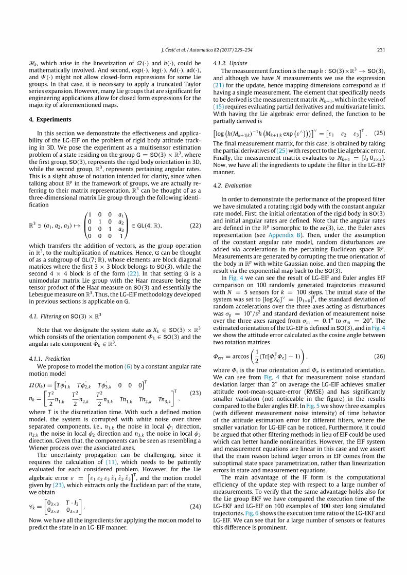
J. Ćesić et al. / Automatica 82 (2017) 226–234 231
Hk, which arise in the linearization of Ω(·) and h(·), could bemathematically involved. And second, exp(·), log(·), Ad(·), ad(·),and Ψ (·) might not allow closed-form expressions for some Liegroups. In that case, it is necessary to apply a truncated Taylorseries expansion. However, many Lie groups that are significant forengineering applications allow for closed form expressions for themajority of aforementioned maps.
4. Experiments
In this section we demonstrate the effectiveness and applica-bility of the LG-EIF on the problem of rigid body attitude track-ing in 3D. We pose the experiment as a multisensor estimationproblem of a state residing on the group G = SO(3) × R3, wherethe first group, SO(3), represents the rigid body orientation in 3D,while the second group, R3, represents pertaining angular rates.This is a slight abuse of notation intended for clarity, since whentalking about Rp in the framework of groups, we are actually re-ferring to their matrix representation. R3 can be thought of as athree-dimensional matrix Lie group through the following identi-fication
R3∋ (a1, a2, a3) →
1 0 0 a10 1 0 a20 0 1 a30 0 0 1
∈ GL(4;R), (22)
which transfers the addition of vectors, as the group operationin R3, to the multiplication of matrices. Hence, G can be thoughtof as a subgroup of GL(7;R), whose elements are block diagonalmatrices where the first 3 × 3 block belongs to SO(3), while thesecond 4 × 4 block is of the form (22). In that setting G is aunimodular matrix Lie group with the Haar measure being thetensor product of the Haar measure on SO(3) and essentially theLebesguemeasure onR3. Thus, the LG-EIFmethodology developedin previous sections is applicable on G.
4.1. Filtering on SO(3)× R3
Note that we designate the system state as Xk ∈ SO(3) × R3
which consists of the orientation component Φk ∈ SO(3) and theangular rate component Φk ∈ R3.
4.1.1. PredictionWe propose to model the motion (6) by a constant angular rate
motion model
Ω(Xk) =T ˙φ1,k T ˙φ2,k T ˙φ3,k 0 0 0
Tnk =
T 2
2n1,k
T 2
2n2,k
T 2
2n3,k Tn1,k Tn2,k Tn3,k
T
,(23)
where T is the discretization time. With such a defined motionmodel, the system is corrupted with white noise over threeseparated components, i.e., n1,k the noise in local φ1 direction,n2,k the noise in local φ2 direction and n3,k the noise in local φ3direction. Given that, the components can be seen as resembling aWiener process over the associated axes.
The uncertainty propagation can be challenging, since itrequires the calculation of (11), which needs to be patientlyevaluated for each considered problem. However, for the Liealgebraic error ε =
ε1 ε2 ε3 ε1 ε2 ε3
T, and the motion modelgiven by (23), which extracts only the Euclidean part of the state,we obtain
Ck =
03×3 T · I303×3 03×3
. (24)
Now, we have all the ingredients for applying the motion model topredict the state in an LG-EIF manner.
4.1.2. UpdateThemeasurement function is themap h : SO(3)×R3
→ SO(3),and although we have N measurements we use the expression(21) for the update, hence mapping dimensions correspond as ifhaving a single measurement. The element that specifically needsto be derived is themeasurementmatrixHk+1, which in the vein of(15) requires evaluating partial derivatives andmultivariate limits.With having the Lie algebraic error defined, the function to bepartially derived islog
h(Mk+1|k)
−1hMk+1|k exp
ε∧
∨=
ε1 ε2 ε3
T. (25)
The final measurement matrix, for this case, is obtained by takingthe partial derivatives of (25)with respect to the Lie algebraic error.Finally, the measurement matrix evaluates to Hk+1 = [I3 03×3].Now, we have all the ingredients to update the filter in the LG-EIFmanner.
4.2. Evaluation
In order to demonstrate the performance of the proposed filterwe have simulated a rotating rigid body with the constant angularrate model. First, the initial orientation of the rigid body in SO(3)and initial angular rates are defined. Note that the angular ratesare defined in the Rp isomorphic to the so(3), i.e., the Euler axesrepresentation (see Appendix B). Then, under the assumptionof the constant angular rate model, random disturbances areadded via accelerations in the pertaining Euclidean space Rp.Measurements are generated by corrupting the true orientation ofthe body in Rp with white Gaussian noise, and then mapping theresult via the exponential map back to the SO(3).
In Fig. 4 we can see the result of LG-EIF and Euler angles EIFcomparison on 100 randomly generated trajectories measuredwith N = 5 sensors for k = 100 steps. The initial state of thesystem was set to [log X0]
∨= [01×6]T, the standard deviation of
random accelerations over the three axes acting as disturbanceswas σp = 10°/s2 and standard deviation of measurement noiseover the three axes ranged from σm = 0.1° to σm = 20°. Theestimated orientation of the LG-EIF is defined inSO(3), and in Fig. 4we show the attitude error calculated as the cosine angle betweentwo rotation matrices
Φerr = arccos12(Tr[ΦT
t Φe] − 1), (26)
where Φt is the true orientation and Φe is estimated orientation.We can see from Fig. 4 that for measurement noise standarddeviation larger than 2° on average the LG-EIF achieves smallerattitude root-mean-square-error (RMSE) and has significantlysmaller variation (not noticeable in the figure) in the resultscompared to the Euler angles EIF. In Fig. 5 we show three examples(with different measurement noise intensity) of time behaviorof the attitude estimation error for different filters, where thesmaller variation for LG-EIF can be noticed. Furthermore, it couldbe argued that other filtering methods in lieu of EIF could be usedwhich can better handle nonlinearities. However, the EIF systemand measurement equations are linear in this case and we assertthat the main reason behind larger errors in EIF comes from thesuboptimal state space parametrization, rather than linearizationerrors in state and measurement equations.
The main advantage of the IF form is the computationalefficiency of the update step with respect to a large number ofmeasurements. To verify that the same advantage holds also forthe Lie group EKF we have compared the execution time of theLG-EKF and LG-EIF on 100 examples of 100 step long simulatedtrajectories. Fig. 6 shows the execution time ratio of the LG-EKF andLG-EIF. We can see that for a large number of sensors or featuresthis difference is prominent.

232 J. Ćesić et al. / Automatica 82 (2017) 226–234
Fig. 4. Comparison of attitude RMSE with respect to increase in measurementnoise standard deviation. The results represent the mean value of the RMSE andone standard deviation of 100 MC runs. We can see that the LG-EIF exhibits smallererror and has more consistent performance over various trajectories.
Fig. 5. Three examples of time behavior of the attitude estimation error through200 steps. The standard deviation for measurement noise was set to σm = 2.5°(top), σm = 5° (middle), σm = 10° (bottom). The attitude RMSE for each filter isgiven in the subfigure titles.
5. Conclusion
In this paper we have proposed a new state estimationalgorithm on Lie groups. We have embedded the LG-EKF with anEIF form for non-linear systems, thus endowing the filter with theinformation forms advantages with regard to multisensor updateand decentralization, while keeping the accuracy of the LG-EKF forstochastic inference on Lie groups. The theoretical development ofthe LG-EIF recursion equationswas presented and the applicabilityof the proposed approach demonstrated on the problem of rigidbody attitude tracking with multiple sensors by setting the stateon the Lie group SO(3) × R3. The first component of the state
Fig. 6. Comparison of LG-EKF and LG-EIF time execution with respect tothe number of measurements in the update step. We can see that after 100measurements the difference becomes extremely prominent. The figure representsmean value of the execution time ratio for 50 Monte Carlo runs.
represented the rigid body orientation in 3D, while the secondcomponent represented the pertaining angular rates. The systemmodel was then set as a constant angular rate model acting onthe state space SO(3)× R3. The results have shown that the filtercan accurately track the rigid body attitude and that on averageit exhibits lower RMSE and more consistent performance than theEuler angles based EIF. Furthermore, the information form of theLG-EIF keeps the multisensor or decentralization computationaladvantage of the update step with respect to the LG-EKF.
Acknowledgments
This work has been supported from the Unity Through Knowl-edge Fund under Grant 24/15 (Cooperative Cloud based Simulta-neous Localization andMapping in Dynamic Environments, cloud-SLAM) and the research has also been carried out within the activ-ities of the Centre of Research Excellence for Data Science and Co-operative Systems supported by theMinistry of Science, Educationand Sports of the Republic of Croatia under Grant 533-19-15-0007.
Appendix A. Lie algebraic error prediction
Proposition 4 (Baker–Campbell–Hausdorff). Given a Lie algebra g,for all a, b ∈ g such that |a∨
| and |b∨| are sufficiently small, the
following identity holds (Hall, 2003):
log (exp (a) exp (b)) = a +
1
0ψ(exp(ad(a)) exp(t ad(b)))(b)dt,
(A.1)
where ψ(z) = z log z/(z − 1).
This is an integral version of the famousBaker–Campbell–Hausdorff(BCH) formula, which is better known in an expanded form
log (exp (a) exp (b)) = a + b +12[a, b]
+112([a, [a, b]] + [b, [b, a]])+ · · · .
(A.2)
Another useful identity used in the derivation of the predictedLie algebraic error is a first-order approximation relation betweenadditive and multiplicative perturbations on matrix Lie groups.Namely, for every a, δ ∈ g and |δ∨
| small, i.e., neglecting thesecond-order terms in |δ∨
|, it holds
exp(a + δ) ≈ exp(a) exp(Ψ (a)δ), (A.3)

J. Ćesić et al. / Automatica 82 (2017) 226–234 233
where Ψ (a) denotes the right Jacobian of the Lie group defined by(9). The latter identity implies the approximation formula
log(exp(−a) exp(a + δ)) = Ψ (a)δ. (A.4)
Now we proceed with the derivation of the Lie algebraic errorprediction. In Section 3.2 we computed the exponential of thepredicted Lie algebraic error εk+1|k at time step k
exp(ε∧
k+1|k) = exp−Ω∧
k
exp
ε∧
k
exp
Ω(Xk)
∧+ n∧
k
,
where we recall Ωk = Ω(Mk) and εk is the Lie algebraic error attime step k. Linearizing the mapΩ atMk we have
exp(ε∧
k+1|k) = exp−Ω∧
k
exp
ε∧
k
exp
Ω∧
k + (Ckεk)∧
+ n∧
k
,
(A.5)
where
Ck =∂
∂εΩ
Mk exp
ε∧
|ε=0.
Using the BCH formula (A.2) by considering only the first fourmembers from the expansion and neglecting O(|ε∧
k , n∧
k |2) terms,
we obtain
z∧
k = logexp
ε∧
k
exp
Ω∧
k + (Ckεk)∧
+ n∧
k
= ε∧
k +Ω∧
k + (Ckεk)∧
+ n∧
k +12[ε∧
k ,Ω∧
k ]
+112
[Ω∧
k , [Ω∧
k , ε∧
k ]]. (A.6)
Inserting (A.6) into (A.5) one has
exp(ε∧
k+1|k) = exp−Ω∧
k
exp(z∧
k ),
thus, using the approximation identity (A.4), the followingexpression holds
ε∧
k+1|k = Ψ (Ωk)ε∧
k + (Ckεk)∧
+ n∧
k +12[ε∧
k ,Ω∧
k ]
+112
[Ω∧
k , [Ω∧
k , ε∧
k ]]
.
Recognizing terms Ψ (Ωk)(Ckεk)∧ and Ψ (Ωk)n∧
k in the predictionformula (8), it remains to discuss terms
Ψ (Ωk)ε∧
k +12[ε∧
k ,Ω∧
k ] +112
[Ω∧
k , [Ω∧
k , ε∧
k ]]
. (A.7)
Evaluating (A.7):
ε∧
k +12[ε∧
k ,Ω∧
k ] +112
[Ω∧
k , [Ω∧
k , ε∧
k ]]
−12
Ω∧
k , ε∧
k +12[ε∧
k ,Ω∧
k ] +112
[Ω∧
k , [Ω∧
k , ε∧
k ]]
+
16
Ω∧
k ,Ω∧
k , ε∧
k +12[ε∧
k ,Ω∧
k ] +112
[Ω∧
k , [Ω∧
k , ε∧
k ]]
−
124
Ω∧
k ,Ω∧
k ,Ω∧
k , ε∧
k +12[ε∧
k ,Ω∧
k ]
+112
[Ω∧
k , [Ω∧
k , ε∧
k ]]
+ · · ·
leads to the expression
ε∧
k + [−Ω∧
k , ε∧
k ] +12[−Ω∧
k , [−Ω∧
k , ε∧
k ]]
+16[−Ω∧
k , [−Ω∧
k , [−Ω∧
k , ε∧
k ]]]
+5
144[−Ω∧
k , [−Ω∧
k , [−Ω∧
k , [−Ω∧
k , ε∧
k ]]]]
+1
288[−Ω∧
k , [−Ω∧
k , [−Ω∧
k , [−Ω∧
k , [−Ω∧
k , ε∧
k ]]]]] + · · · ,
which can be finally recognized as an approximation of
exp(ad(−Ω∧
k ))ε∧
k = Ad(exp(−Ω∧
k ))ε∧
k .
This finishes the derivation of the Lie algebraic error prediction.
Appendix B. The special orthogonal group SO(3)
The SO(3) group is a set of orthogonal matrices with determi-nant one, whose elements geometrically represent rotations. Rota-tions in 3D can also be representedwith an Euler vector (also calledthe axis–angle notation), where a vector φ = [φ1 φ2 φ3]
T∈ R3 de-
notes a rotation about the unit vector φ/|φ| by the angle |φ|. Aninteresting notion is that the Lie algebra so(3) is given as the skewsymmetric matrix of the Euler vector
φ∧=
0 −φ3 φ2φ3 0 −φ1
−φ2 φ1 0
∈ so(3), (B.1)
where (·)∧ : R3→ so(3) and its inverse, (·)∨ : so(3) → R3, follow
trivially. The exponential map exp : so(3) → SO(3) is given asBarfoot and Furgale (2014)
exp(φ∧) = cos(|φ|)I3 + (1 − cos(|φ|))φφT
|φ|2+ sin(|φ|)
φ∧
|φ|. (B.2)
Furthermore, for an Φ ∈ SO(3), the matrix logarithm, performingmapping log : SO(3) → so(3), is given as
log(Φ) =
γ
2 sin(γ )(Φ − ΦT ), if γ = 0
0, if γ = 0,(B.3)
where 1+ 2 cos γ = Tr(Φ) and Tr( · ) designates the matrix trace.The adjoint operators Ad and ad for SO(3) are respectively givenas
Ad(Φ) = Φ and ad(φ∧) = φ∧. (B.4)
Given the above definitions, we have all the needed ingredients touse the SO(3) group within the LG-EIF.
References
Bailey, T., Upcroft, B., & Durrant-Whyte, H. (2006). Validation gating for non-linearnon-Gaussian target tracking. In International conference on information fusion,(pp. 1–6).
Barfoot, T. D., & Furgale, P. T. (2014). Associating uncertainty with three-dimensional poses for use in estimation problems. IEEE Transactions on Robotics,30(3), 679–693.
Battistelli, G., & Chisci, L. (2016). Stability of consensus extended Kalman filter fordistributed state estimation. Automatica, 68, 169–178.
Bourmaud, G., Mégret, R., Arnaudon, M., & Giremus, A. (2015). Continuous-discreteextended Kalman filter on matrix Lie groups using concentrated Gaussiandistributions. Journal of Mathematical Imaging and Vision, 51(1), 209–228.
Bourmaud, G., Mégret, R., Giremus, A., & Berthoumieu, Y. (2013). Discrete extendedKalman filter on Lie groups. In European signal processing conference, EUSIPCO,(pp. 1–5).
Campbell, M. E., & Whitacre, W. W. (2007). Cooperative tracking using visionmeasurements on SeaScan UAVs. IEEE Transactions on Control SystemsTechnology, 15(4), 613–626.
Ćesić, J., Joukov, V., Petrović, I., & Kulić, D. (2016). Full body human motionestimation on Lie groups using 3D marker position measurements. In IEEE-RASinternational conference on humanoid robots, Humanoids.
Ćesić, J.,Marković, I., Cvišić, I., & Petrović, I. (2016). Radar and stereo vision fusion formultitarget tracking on the special Euclidean group. Robotics and AutonomousSystems,.
Chirikjian, G. S., & Kyatkin, A. B. (2000). Engineering applications of noncommutativeHarmonic analysis: With emphasis on rotation and motion groups. CRC Press.
Engel, J., Sch, T., & Cremers, D. (2014). LSD-SLAM: Direct monocular SLAM. InEuropean conference on computer vision, ECCV, (pp. 834–849).
Eustice, R. M., Singh, H., & Leonard, J. J. (2006). Exactly sparse delayed-state filtersfor view-based SLAM. IEEE Transactions on Robotics, 22(6), 1100–1114.
Forster, C., Carlone, L., Dellaert, F., & Scaramuzza, D. (2015). IMU preintegrationon manifold for efficient visual-inertial maximum-a-posteriori estimation.In Robotics: Science and systems (p. 9).

234 J. Ćesić et al. / Automatica 82 (2017) 226–234
Fu, Y., Ling, Q., & Tian, Z. (2012). Distributed sensor allocation for multi-targettracking in wireless sensor networks. IEEE Transactions on Aerospace andElectronic Systems, 48(4), 3538–3553.
Gilitschenski, I., Kurz, G., Julier, S.J., & Hanebeck, U.D. (2014). A new probabilitydistribution for simultaneous representation of uncertain position andorientation. In International conference on information fusion, FUSION, (p. 7).
Grocholsky, B., Makarenko, A., & Durrant-Whyte, H. (2003). Information-theoreticcoordinated control of multiple sensor platforms. In International conference onrobotics and automation, Vol. 1, (ICRA). (pp. 1521–1526). IEEE.
Hall, B. C. (2003). Lie groups, Lie algebras, and representations: An elementaryintroduction. Springer-Verlag.
Hertzberg, C.,Wagner, R., Frese, U., & Schröder, L. (2013). Integrating generic sensorfusion algorithms with sound state representations through encapsulation ofmanifolds. Information Fusion, 14(1), 57–77.
Khosravian, A., Trumpf, J., Mahony, R., & Hamel, T. (2015). State estimationfor invariant systems on Lie groups with delayed output measurements.Automatica, 68, 254–265.
Kümmerle, R., Grisetti, G., Rainer, K., Strasdat, H., Konolige, K., & Burgard, W.(2011). g2o: A general framework for graph optimization. In IEEE internationalconference on robotics and automation, ICRA, (pp. 3607–3613).
Kurz, G., Gilitschenski, I., & Hanebeck, U.D. (2014). The partially wrapped normaldistribution for SE(2) estimation. In International conference on multisensorfusion and information integration for intelligent systems, no. 2, (p. 8).
Lee, D.-J. (2008). Nonlinear estimation and multiple sensor fusion using unscentedinformation filtering. IEEE Signal Processing Letters, 15(2), 861–864.
Liu, G., Wörgötter, F., & Markelić, I. (2012). Square-root sigma-point informationfiltering. IEEE Transactions on Automatic Control, 57(11), 2945–2950.
Maybeck, P. S. (1979). In A. Press (Ed.), Stochastic models, estimation and control.Volume I..
Mur-Artal, R., Montiel, J. M. M., & Tardos, J. D. (2015). ORB-SLAM: a versatileand accurate monocular slam system. IEEE Transactions on Robotics, 31(5),1147–1163.
Murray, R. M., Li, Z., & Sastry, S. S. (1994). A mathematical introduction to roboticmanipulation. Ann Arbor, MI: CRC.
Nettleton, E., Durrant-Whyte, H.F., & Sukkarieh, S. (2003). A robust architecture fordecentralised data fusion. In International conference on advanced robotics, ICAR.
Nielsen, F., & Garcia, V. (2009). Statistical exponential families: A digest with flashcards. Computing Research Repository. arXiv:0911.4863.
Onel, T., Ersoy, C., & Delic, H. (2009). Information content-based sensor selectionand transmission power adjustment for collaborative target tracking. IEEETransactions on Mobile Computing , 8(8), 1103–1116.
Pakki, K., Chandra, B., & Postlethwaite, I. (2013). Square root cubature informationfilter. IEEE Sensors Journal, 13(2), 750–758.
Rao, B. S. Y., Durrant-Whyte, H. F., & Sheen, J. A. (1993). A fully decentralized multi-sensor system for tracking and surveillance. International Journal of RoboticsResearch, 12(1), 20–44.
Ros, G., Guerrero, J., Sappa, A. D., Ponsa, D., & Lopez, A. M. (2013). VSLAM poseinitialization via Lie groups and Lie algebras optimization. In Internationalconference on robotics and automation, (ICRA). (pp. 5740–5747). IEEE.
Selig, J. M. (1996). Geometrical methods in robotics. New York: Springer-Verlag.Thrun, S., Burgard, W., & Fox, D. (2006). Probabilistic robotics. The MIT Press.Thrun, S., Liu, Y., Koller, D., Ng, A. Y., Ghahramani, Z., & Durrant-Whyte, H. (2004).
Simultaneous localization and mapping with sparse extended informationfilters. International Journal of Robotics Research, 23(7–8), 693–716.
Vercauteren, T., & Wang, X. (2005). Decentralized sigma-point information filtersfor target tracking in collaborative sensor networks. IEEE Transactions on SignalProcessing , 53(8), 2997–3009.
Wang, Y., & Chirikjian, G. S. (2006a). Error propagation on the Euclidean groupwithapplications to manipulator kinematics. IEEE Transactions on Robotics, 22(4),591–602.
Wang, Y., & Chirikjian, G. (2006b). Error propagation on the Euclidean group withapplications to manipulator kinematics. IEEE Transactions on Robotics, 22(4),591–602.
Wang, S., Feng, J., & Tse, C. K. (2014). A class of stable square-root nonlinearinformation filters. IEEE Transactions on Automatic Control, 59(7), 1893–1898.
Wolfe, K. C., Mashner, M., & Chirikjian, G. S. (2011). Bayesian fusion on Lie groups.Journal of Algebraic Statistics, 2(1), 75–97.
Woodbury, M. A. (1950). Inverting Modified Matrices, ser. Statistical Research GroupMemorandum Reports. Princeton, NJ: Princeton University, no. 42.
Zhang, Y., Chai Soh, Y., & Chen, W. (2005). Robust information filter fordecentralized estimation. Automatica, 41(12), 2141–2146.
Josip Ćesić has received his B.Sc. andM.Sc. degrees (MagnaCum Laude) in Electrical Engineering and InformationTechnology from University of Zagreb Faculty of ElectricalEngineering and Computing (UNIZG-FER) in 2011 and2013, respectively. He finished part of the master studiesat Chalmers University of Technology, Sweden. He isemployed as a research assistant at the Department ofControl and Computer Engineering at UNIZGG-FER sinceApril 2013. During the undergraduate studies he receivedDean’s Award and Special Dean’s Award for achievementson the first year of studies and the overall B.Sc. level,
respectively. During the graduate studies he received the Rector’s Award andSpecial Rector’s Award for practical applications in the fields of robotics and controlsystems, and was awarded with several scholarships. His main research interestsare in the areas of autonomous systems, mobile robotics, estimation theory andsensor processing.
Ivan Marković is an Assistant Professor at the Universityof Zagreb Faculty of Electrical Engineering and Computing,Croatia (UNIZG-FER). He received the M.Sc. and Ph.D.degrees in Electrical Engineering from the UNIZG-FER in2008 and 2014, respectively. During his undergraduateand graduate studies he was awarded with the ‘‘INETEC’’award (2007), ‘‘Josip Lončar’’ faculty award (2008), andwith scholarship from the CroatianMinistry of Science andEducation for the best students (2003–2008). In 2014 forhis Ph.D. thesis he was awarded with the Silver Plaque‘‘Josip Lončar’’ faculty award for outstanding doctoral
dissertation and particularly successful scientific research. He is a member of theInstitute of Electrical and Electronics Engineers (IEEE). He was a visiting researcherat INRIA Rennes-Bretagne Atlantique, Rennes, France, Lagadic group (Prof. FrançoisChaumette). His research interests are mobile robotics, especially detection andtracking of moving objects and speaker localization.
Mario Bukal received the M.S. degree in Applied Math-ematics from the University of Zagreb in 2008 and thePh.D. in Applied Mathematics from the Vienna Universityof Technology in 2012. From2012he iswith theUniversityof Zagreb Faculty of Electrical Engineering and Computing,where he is currently an Assistant Professor. His researchfocus is in applied mathematics, in particular, mathemati-cal and numerical analysis of higher-order diffusion equa-tions, and homogenizations and dimension reduction innonlinear elasticity theory. His research interests also in-clude information fusion with application to robotic sys-
tems.
Ivan Petrović (www.unizg.fer.hr/ivan.petrovic) is theHead of the Laboratory for Autonomous Systems andMobile Robotics (http://lamor.fer.hr) and the Centre ofResearch Excellence for Advance Cooperative Systems-ACROSS (http://across.fer.unizg.hr). He has more than 30years of professional experience in R&D of automaticcontrol theory and its applications. In the last fifteenyears his research is focused on the advanced control andestimation techniques and their application in control andnavigation of autonomous mobile robots and vehicles. Hepublished about 50 journal papers and more than 180
conference papers. Results of his research effort have been implemented in severalindustrial products. He is a member of IEEE, IFAC-Vice Chair of TC on Robotics andFIRA-Executive committee. He is amember of the Croatian Academy of Engineering.

114 publications
publication 7
J. Ćesić, I. Marković, I. Cvišić and I. Petrović. Radar and stereo vision fusion for multitarget
tracking on the special Euclidean group. Robotics and autonomous systems, 83:338–348,
2016.

Robotics and Autonomous Systems 83 (2016) 338–348
Contents lists available at ScienceDirect
Robotics and Autonomous Systems
journal homepage: www.elsevier.com/locate/robot
Radar and stereo vision fusion for multitarget tracking on the specialEuclidean group
Josip Ćesić ∗, Ivan Marković, Igor Cvišić, Ivan PetrovićUniversity of Zagreb, Faculty of Electrical Engineering and Computing, Department of Control and Computer Engineering, Unska 3, 10000 Zagreb, Croatia
h i g h l i g h t s
• Radar and stereo camera integration for tracking in ADAS.• Detection and tracking of moving objects by filtering on matrix Lie groups.• State space formed as a product of two special Euclidean groups.• Employed banana-shaped uncertainties typical for range-bearing sensors and vehicles in motion.• JIPDA filter for multitarget tracking on matrix Lie groups.
a r t i c l e i n f o
Article history:Available online 12 May 2016
Keywords:Advanced driver assistance systemsDetection and tracking of moving objectsJoint integrated probabilistic dataassociation
RadarStereo camera
a b s t r a c t
Reliable scene analysis, under varying conditions, is an essential task in nearly any assistance orautonomous system application, and advanced driver assistance systems (ADAS) are no exception.ADAS commonly involve adaptive cruise control, collision avoidance, lane change assistance, traffic signrecognition, and parking assistance—with the ultimate goal of producing a fully autonomous vehicle.The present paper addresses detection and tracking of moving objects within the context of ADAS. Weuse a multisensor setup consisting of a radar and a stereo camera mounted on top of a vehicle. Wepropose to model the sensors uncertainty in polar coordinates on Lie Groups and perform the objectsstate filtering on Lie groups, specifically, on the product of two special Euclidean groups, i.e., SE(2)2. To thisend, we derive the designed filter within the framework of the extended Kalman filter on Lie groups. Weassert that the proposed approach results with more accurate uncertainty modeling, since used sensorsexhibit contrastingmeasurement uncertainty characteristics and the predicted targetmotions result withbanana-shapeduncertainty contours.Webelieve that accurate uncertaintymodeling is an importantADAStopic, especially when safety applications are concerned. To solve the multitarget tracking problem, weuse the joint integrated probabilistic data association filter andpresent necessarymodifications in order touse it on Lie groups. The proposed approach is tested on a real-world dataset collected with the describedmultisensor setup in urban traffic scenarios.
© 2016 Elsevier B.V. All rights reserved.
1. Introduction
Reliable comprehension of the surrounding environment,under varying conditions, is an essential task in nearly anyassistance or autonomous system application. Since the advent
This work has been supported by the Unity Through Knowledge Fund under theproject Cooperative Cloud based Simultaneous Localization and Mapping in DynamicEnvironments and the European Regional Development Fund under the projectAdvanced Technologies in Power Plants and Rail Vehicles.∗ Corresponding author.
E-mail addresses: [email protected] (J. Ćesić), [email protected](I. Marković), [email protected] (I. Cvišić), [email protected] (I. Petrović).
of autonomous vehicle research, scientific community has beenactively engaged in developing advanced driver assistance systems(ADAS). ADAS commonly involve adaptive cruise control, collisionavoidance, lane change assistance, traffic sign recognition, andparking assistance—with the final goal being a fully autonomousvehicle. ADAS have been in the focus of research for a few decades,intended to enhance the safety and reduce the possibility of ahuman error as a cause of road accidents [1]. An essential taskin numerous ADAS applications is the detection and tracking ofmoving objects (DATMO), since it allows the vehicle to be awareof dynamic objects in its immanent surrounding and predict theirfuture behavior. Since the robustness of such an application undervarying environmental conditions represents a complex challenge,
http://dx.doi.org/10.1016/j.robot.2016.05.0010921-8890/© 2016 Elsevier B.V. All rights reserved.

J. Ćesić et al. / Robotics and Autonomous Systems 83 (2016) 338–348 339
it has become clear that there does not exist such a sensing systemthat could solely deliver full information required for adequatequality of ADAS applications [2].
Given that, ADAS commonly rely on using complementarysensing systems: vision,millimeter-wave radars, laser range finder(LRF) or combinations thereof. Radar units are able to produceaccurate measurements of the relative speed and distance to theobjects. LRF have higher lateral resolution than the radars and,besides accurate object distance, they can detect the occupancyarea of an object and provide detailed scene representation [3].Regarding the robustness, radar units are more robust to rain, fog,snow, and similar conditions that may cause inconveniences forLRF; but, they produce significant amount of clutter as a drawback.Vision-based sensing systems can also provide accurate lateralmeasurements and wealth of other information from images,thus provide an effective supplement to ranging-based sensorroad scene analysis. As an example, a stereo vision sensor canprovide target detection with high lateral resolution and lesscertain range, while usually bringing enough information foridentification and classification of objects, whereas radar canprovide accurate measurements of range and relative speed.Given the complementarity of radars and vision systems, thiscombination is commonly used in research for ADAS applications.For example, works based on a monocular camera use radar forfinding regions of interest in the image [4–7], process separatelyimage and radar data [8–10], use motion stereo to reconstructobject boundaries [11,12], while [13,14] use directly stereocameras. Employingmultiple sensors, and consequently exploitingtheir differentmodalities, requires fusion of the sensing systems atappropriate levels. Depending on the approach, fusion can roughlytake place at three levels: before objects detection (low level) [13,14], at the objects’ detection level (fused list of objects) [12,10], orat the state level (updating the states of objects in the list for eachsensor system) [9,8,15].
Since in ADAS applications sensors with very different charac-teristics are used; e.g. radar with higher lateral uncertainty, butprecise range estimation, and stereo camera with low lateral un-certainty but higher range imprecision, question arises on howto faithfully model the uncertainty of the state, estimated asyn-chronously with such sensors. Moreover, since in urban scenar-ios targets can exhibit varying dynamic behavior, a flexible motionmodel, capable of capturing the maneuvering diversity, should beused.
In the present paper, which is a continuation of our previouswork presented in [16], we use a combination of a radar anda stereo vision system to perform the target tracking task.Our previous work focused on developing an appearance-baseddetection approach, while this paper deals with the tracking partof the DATMO procedure and uses a motion-based detectiontechnique. Given the previous discussion, our first contributionis in modeling radar and stereo measurements arising in polarcoordinates as members of Lie Groups SO(2) × R1, and inestimating the target state as the product of two special Euclideanmotion groups SE(2) × SE(2) = SE(2)2. This is performed withinthe framework of the extended Kalman filter on Lie groups, whichwe derive for the proposed system design. Furthermore, the targetmotion model also resides on the same group product and assuch will yield the required model flexibility. This will not onlyenable us to correctly model sensor uncertainties, but also to havehigher diversity in the uncertainty representation of the stateestimates. For example, besides the standard Gaussian ellipticallyshaped uncertainty, proposed representation also supports the socalled banana-shaped uncertainties. The second contribution of thepaper is the adaptation of the joint integrated probabilistic dataassociation (JIPDA) filter for multitarget on the SE(2)2. To the bestof the author’s knowledge, this is the first use of a filtering on LieGroups for a multitarget tracking application.
The rest of the paper is organized as follows. Section 2 presentsrelated work and the present paper’s contributions. Section 3presents mathematical background of the LG-EKF, while Section 4derives the proposed asynchronous LG-EKF on SE(2)2 with polarmeasurements. The multitarget tracking with JIPDA filter onSE(2)2 is described in Sections 5 and 6 presents the real-worldexperimental results. In the end, Section 7 concludes the paper.
2. Related work and progress beyond
Several distinct research fields relate to the study presented inthis paper. These include the state estimation on Lie groups, mul-titarget tracking, stereo vision- and radar-based signal processing.We focus our overview of related work in the pertinent fields byconsidering results relevant to the present application.
To detect objects of interest, vision algorithms can resortto (i) appearances at a single time step, and (ii) motion overseveral frames [2]. In [17] authors employ detection procedurebased on appearances in the disparity space, where clusteringand extraction of moving objects are performed. The work in [18]focuses on ego-motion estimation, while moving objects stemfrom clustering the estimated motions in the filtered point cloud.Scene flow, i.e., the motion in 3D from stereo sequences, wasused in [19,20], where adjacent points describing similar flow areconsidered to belong to a single rigid object. In [21] objects are alsoextracted from the scene flow, after which clustering is performed,and the iterative closest point algorithm is used to determine thevehicles’ pose. Approach in [22] combines depth and optical flow-based clustering with an active learning-based method. In [23]pedestrians were isolated from the stereo point cloud and theirpose estimated using a visibility-based 3Dmodel, which is capableof predicting occlusions and using them in the detection process.
Concerning radar and stereo vision integration, in [14] approachbased on fitting themodel of a vehicle contour to both stereo depthimage and radar readings was presented. First, the algorithm fitsthe contour from stereo depth information and finds the closestpoint of the contour with respect to the vision sensor. Second, itdetermines the closest point of the radar observation and fusesradar’s and vision’s closest points. By translating the initially fittedcontour to the fused closest point, the resulting contour is obtainedand located. Another low level integration approachwas presentedin [13]. In particular, the edge map of the stereo image is split intolayers corresponding to different target depths so that the layerscontain edge pixels of targets at different depth ranges. Hence, theoriginal multitarget segmentation task is decomposed into severalsingle target segmentation tasks on each depth-based layer, thuslowering the computational costs of the segmentation.
In the present paper each sensor reports its detectionsindependently. To estimate the interim vehicle displacement, weuse our visual stereo odometry algorithm (named SOFT) presentedin [24]. Features not conforming to the computed displacementare considered as moving objects and are grouped together toyield measurements which are then fed to the tracking algorithm.In that respect our approach would fall within the motion-baseddetection approaches. The radar sensor complements detectionsfrom the stereo camera, and reports to the tracking algorithm a listof possible obstacle detections.
Irrespective of the used sensor setup, in traffic scenarios onemust address the problem of multitarget tracking. This entailsestimation (tracking) of each target’s state and dealing withthe problem of associating correct measurements to the trackedtargets in cluttered environments, i.e. solving the data associationproblem. Commonly, for state estimation the Kalman filter andits non-linear variants are used. However, in order to achievethe proposed state uncertainty representation and motion modelflexibility, in the present paper we use the extended Kalman filter
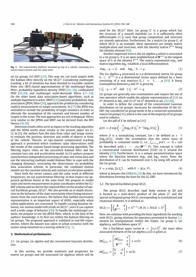
340 J. Ćesić et al. / Robotics and Autonomous Systems 83 (2016) 338–348
Fig. 1. The experimental platform mounted on top of a vehicle, consisting of astereo camera system and two radar units.
on Lie groups (LG-EKF) [25]. This way we can track targets withthe Kalman filter directly on the SE(2)2. Considering multitargettracking, a lot of attention has been devoted to tractable randomfinite sets (RFS)-based approximations of the multitarget Bayesfilter: probability hypothesis density (PHD) [26–28], cardinalizedPHD [29,30], and multitarget multi-Bernoulli filters [31–34].On the other hand, data association-based algorithms, such asmultiple hypothesis tracker (MHT) [35] and joint probabilistic dataassociation (JPDA) filter [36], approach the problem by consideringexplicit measurement-to-target associations. In [37] the JPDA wasextended to include the probability of target existence in order toalleviate the assumption of the constant and known number oftargets in the scene. The two approaches are not orthogonal; filtersvery similar to the JIPDA and MHT can be derived from the RFStheory [38,39].
Detection results often serve as inputs to the tracking algorithmand the ADAS works most similar to the present paper are [8,9]. In [8], the authors fuse the data from radar and image sensorto estimate the position, direction and width of objects in frontof the vehicle. Therein, an ego-motion compensated trackingapproach is presented which combines radar observations withthe results of the contour-based image processing algorithm. Thefiltering aspect relies on the unscented Kalman filter and theconstant turn rate and acceleration model. In [9] authors proposeasynchronous independent processing of radar and vision data anduse the interacting multiple model Kalman filter to cope with thechanging dynamics, associating the observations via probabilitydata association scheme. In particular, the combined motionmodels are the constant velocity and constant accelerationmodels.
Since both the stereo camera and the radar work at differentfrequencies, we use asynchronous filtering; in that respect our ap-proach performs fusion at the state level. We propose to modelradar and stereomeasurements in polar coordinateswithin the LG-EKF scheme andwederive the required filter on the product of spe-cial Euclidean groups, SE(2)2. We also provide an in-depth discus-sion on the behavior of the state uncertaintywhen fusingmeasure-ments from the used sensors. We believe that faithful uncertaintyrepresentation is an important aspect of ADAS, especially whensafety applications are concerned. To handle varying dynamic be-havior, ourmotionmodel will reside on SE(2)2, since it can capturewell a wide range of behavior [40]. To handle the multitarget sce-nario, we propose to use the JIPDA filter, which, to the best of theauthors’ knowledge, is its first use within the Kalman filtering onLie groups. The proposed approach is validated in real-life exper-iments, where the dataset was taken in urban scenarios with thesensor setup mounted on a moving vehicle (Fig. 1).
3. Mathematical preliminaries
3.1. Lie groups, Lie algebra and the concentrated Gaussian distribu-tion
In this section, we provide notations and properties formatrix Lie groups and the associated Lie algebras which will be
used for the SE(2)2 filter. Lie group G′ is a group which hasthe structure of a smooth manifold (i.e. it is sufficiently oftendifferentiable [41]) such that group composition and inversionare smooth operations. Furthermore, for a matrix Lie group G, ofwhich SE(2) is an example, these operations are simply matrixmultiplication and inversion, with the identity matrix In×n beingthe identity element [42].
Another important term is the Lie algebra gwhich is associatedto a Lie group G. It is an open neighborhood of 0n×n in the tangentspace of G at the identity In×n. The matrix exponential expG andmatrix logarithm logG establish a local diffeomorphism
expG : g → G and logG : G → g. (1)
The Lie algebra g associated to a p-dimensional matrix Lie groupG ⊂ Rn×n is a p-dimensional vector space defined by a basisconsisting of p real matrices Ei, i = 1, . . . , p [43]. A linearisomorphism between g and Rp is given by
[·]∨
G : g → Rp and [·]∧
G : Rp→ g. (2)
Lie groups are generally non-commutative and require the use oftwo operators which enable the adjoint representation of (i) G onRp denoted as AdG and (ii) Rp on Rp denoted as adG [42,44].
In order to define the concept of the concentrated Gaussiandistribution on Lie groups, necessary for introduction of the LG-EKF, the considered Lie group needs to be a connected unimodularmatrix Lie group [45],which is the case of themajority of Lie groupsused in robotics.
Let the pdf of X be defined as [46]
p(X) = β exp
−12[logG(X)]∨
T
G P−1[logG(X)]∨G
, (3)
where β is a normalizing constant. Let ϵ be defined as ϵ ,[logG(X)]∨G . Under the assumption that the entire mass ofprobability is contained inside G, i.e.,
Rn×n\G p(X) = 0, ϵ can
be described with ϵ ∼ NRp(0p×1, P). This concept is calleda concentrated Gaussian distribution (CGD) on G around theidentity [25]. Furthermore, it is a unique parametrization spacewhere the bijection between expG and logG exists. Now, thedistribution of X can be translated over G by using left action ofthe Lie group
X = µ expG[ϵ]∧G
, with X ∼ G(µ, P), (4)
where G denotes the CGD [46,25]. By this, we have introduced thedistribution forming the base for the LG-EKF.
3.2. The Special Euclidean group SE(2)
The group SE(2) describes rigid body motion in 2D andis formed as a semi-direct product of the plane R2 and thespecial orthogonal group SO(2) corresponding to translational androtational elements. It is defined as
SE(2) =
R t
01×1 1
∈ R3×3
| R, t ∈ SO(2) × R2
. (5)
Now,we continuewith providing the basic ingredients forworkingwith SE(2), giving relations for operators presented in Section 3.1,needed for manipulations within the triplet: Lie group G, Liealgebra g, and Euclidean space Rp.
For a Euclidean space vector x =x y θ
T , the most oftenassociated element of the Lie algebra se(2) is given as
[x]∧SE(2) =
[x]∧SO(2)xy
01×2 0
∈ se(2) (6)
[x]∧SO(2) =
0 −θθ 0
∈ so(2). (7)

J. Ćesić et al. / Robotics and Autonomous Systems 83 (2016) 338–348 341
Their inverses, [·]∨SE(2) and [·]∨
SO(2), follow trivially from the relations(6) and (7), respectively.
The exponential map for the SE(2) group is given as
expSE(2)([x]∧
SE(2)) =
expSO(2)([θ ]∧
SO(2))txty
01×2 1
∈ SE(2) (8)
expSO(2)([θ ]∧
SO(2)) =
cos θ − sin θsin θ cos θ
∈ SO(2) (9)
tx =1θ[x sin θ + y(−1 + cos θ)] (10)
ty =1θ[x(1 − cos θ) + y sin θ ] . (11)
For T = R, t ∈ SE(2), the logarithmic map is
logSE(2)(T ) =
vθ
∧
SE(2)∈ se(2) (12)
θ = logSO(2)(R) = atan2(R21, R11) (13)
v =θ
2(1 − cos θ)
sin θ 1 − cos θ
cos θ − 1 sin θ
t . (14)
The Adjoint operator AdG used for representing T ∈ SE(2) on R3 isgiven as
AdSE(2)(T ) =
R Jt
01×2 1
with J =
0 1
−1 0
, (15)
while the adjoint operator adG for representing x ∈ R3 on R3 isgiven by
adSE(2)(x) =
−θ J Jv01×2 1
, (16)
where v = [x y]T ∈ R2. Given the definitions above, we have allthe needed ingredients for using the SE(2) motion group withinthe proposed approach.
4. Second order rigid body motion estimation
4.1. State space construction
As a rigid body, vehicle’s state can be well described employingthe rigid body motion group. Furthermore, when consideringvelocities of such an object, we can also represent these higherorder moments by using the same motion group. Following therigid body equivalent of the constant velocity motion model [47],here we model the vehicle by constructing the state space G asthe Cartesian (direct) product of the two matrix Lie group SE(2)members [40]
SE(2) × SE(2) = SE(2)2. (17)
The first SE(2) member is the position component, while thesecond one contributes the velocity components. This can beregarded as a white noise acceleration model [47] on the SE(2)group. Considering vehicle tracking applications, in contrast toother well establishedmotionmodels—constant velocity, constantturn rate and velocity, constant curvature and velocity [48,49]—the SE(2)2 motion model provides more artificial flexibility.This flexibility is manifested through including the holonomicbehavior over all three velocity components, i.e., the longitudinal,lateral, and rotational velocities, which have Wiener processcharacterization [47]. Such flexibility provides the ability todescribe motion of objects appearing in ADAS, e.g., vehicles,motorcycles and pedestrians, and hence is appropriate for usagein our particular DATMO focused application.
Matrix Lie group composition and inversion are simple matrixmultiplication and inversion, hence for all the calculations dealingwith operations on G, we can use the symbolic representationconstructed by placing the two SE(2) members of G blockdiagonally. The Lie algebra associated to the Lie group G is denotedas g = se(2) × se(2). The term [x]∧G is also constructed by placingboth se(2)members on themain diagonal, and correspondingly theexponential map on such G is as well formed block diagonally. Formore details on the construction and symbolical representation ofthe groups of interest, please confer [40] where the state modelwas first proposed.
4.2. Motion model and prediction
The motion model satisfies the following equation
Xk+1 = f (Xk, nk) = Xk expG
[Ωk + nk]
∧
G
, (18)
where Xk ∈ G is the state of the system at time k,G is a p-dimensional Lie group, nk ∼ NRp(0p×1,Qk) is white Gaussian noiseand Ωk = Ω(Xk) : G → Rp is a non-linear C2 function. Ifthe posterior distribution at step k − 1 follows the concentratedGaussian distribution on matrix Lie Groups as G(µk−1, Pk−1). Thepredicted mean is given by [25]
µk+1|k = µk expG
[Ωk]
∧
G
. (19)
We model the motion (18) by [40]
Ω(Xk) =Tvxk Tvyk Tωk 0 0 0
T∈ R6, (20)
nk =
T 2
2nxk
T 2
2nyk
T 2
2nωk Tnxk Tnyk Tnωk
T∈ R6.
With this model, the system is corrupted with white noise overthree components, i.e. nx is the noise in the local x direction, ny isthe noise in local y direction and nw is the noise in the rotationalcomponent.
Formula for propagating the covariance of ϵk+1|k through thegeneral motion model (18) is given as in [25]
Pk+1|k = FkPkF Tk + ΦG(Ωk)QkΦG(Ωk)
T , (21)
where the operator Fk, a matrix Lie group equivalent to theJacobian of f (Xk, nk), and ΦG, are evaluated as
Fk = AdG
expG
[−Ωk]
∧
G
+ ΦG(Ωk)Ck
ΦG(v) =
∞m=0
(−1)m
(m + 1)!adG(v)m, v ∈ Rp
Ck =∂
∂ϵΩµk expG
[ϵ]∧G
|ϵ=0 .
(22)
The covariance propagation is challenging since it requirescalculation of (22). The final expression for Ck is thus given as
Ck =
03×3T cosωk −T sinωk 0T sinωk T cosωk 0
0 0 T03×3 03×3
. (23)
The complete derivation ofCk is given in [40]. The adjoint operatorsAdG and adG are also formed block diagonally.
The last needed ingredient is the process noise covariance ma-trix Qk. In the present paper, we perform sensor fusion in an asyn-chronousmannerwith the arrival of eachmeasurement. Hence,weproceed by defining the process to follow continuous white noiseacceleration model (CWNA) over the three components discussed
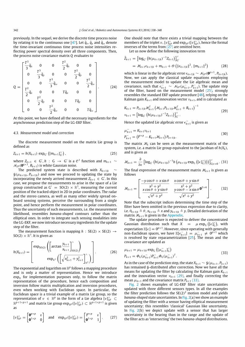
342 J. Ćesić et al. / Robotics and Autonomous Systems 83 (2016) 338–348
previously. In the sequel, we derive the discrete time process noiseby relating it to the continuous one [47]. Let qx, qy and qω denotethe time-invariant continuous time process noise intensities re-flecting power spectral density over all three components. Then,the process noise covariance matrix Q evaluates to
Q =
T 3
3qx 0 0
T 2
2qx 0 0
0T 3
3qy 0 0
T 2
2qy 0
0 0T 3
3qω 0 0
T 2
2qω
T 2
2qx 0 0 T qx 0 0
0T 2
2qy 0 0 T qy 0
0 0T 2
2qω 0 0 T qω
. (24)
At this point, we have defined all the necessary ingredients for theasynchronous prediction step of the LG-EKF filter.
4.3. Measurement model and correction
The discrete measurement model on the matrix Lie group isdefined as
Zk+1 = h(Xk+1) expG′
[mk+1]
∧
G′
, (25)
where Zk+1 ∈ G′, h : G → G′ is a C1 function and mk+1 ∼
NRq(0q×1, Rk+1) is white Gaussian noise.The predicted system state is described with Xk+1|k ∼
G(µk+1|k, Pk+1|k) and now we proceed to updating the state byincorporating the newly arrived measurement Zk+1 ∈ G′. In thiscase, we propose the measurements to arise in the space of a Liegroup constructed as G′
= SO(2) × R1, measuring the currentposition of the tracked object in 2D in polar coordinates. The radarand the stereo camera, as well as many other widely spread on-board sensing systems, perceive the surrounding from a singlepoint, and hence perform the measurement in polar coordinates.Thus the uncertainty of such measurements, i.e. the measurementlikelihood, resembles banana-shaped contours rather than theelliptical ones. In order to integrate such sensing modalities intothe LG-EKF,wenow introduce necessary ingredients for the updatestep of the filter.
The measurement function is mapping h : SE(2) × SE(2) →
SO(2) × R1. It is given as
h(Xk+1) =
expSO(2)
arctan
yk+1
xk+1
∧
SO(2)
expR1
x2k+1 + y2k+1
∧
R1
. (26)
The exponential and logarithm onRp follows amapping procedureand is only a matter of representation. Hence we introduceexpR for implementation purposes only, to follow the matrixrepresentation of the procedure, hence each composition andinversion follow matrix multiplication and inversion procedures,even when working with Euclidean space. In particular, theEuclidean space is a trivial example of a matrix Lie group, so therepresentation of v ∈ Rp in the form of a Lie algebra [v]
∧
Rp ⊂
Rp+1×p+1 and matrix Lie group expRp([v]∧
Rp) ⊂ Rp+1×p+1 is givenas
[v]∧
Rp =
0p×p v
01×p 0
and expRp([v]
∧
Rp) =
Ip×p v
01×p 1
. (27)
One should note that there exists a trivial mapping between themembers of the triplet v, [v]
∧
Rp and expRp([v]∧
Rp), hence the formalinverses of the terms from (27) are omitted here.
Let us now define the following innovation term
Zk+1 =logG′
h(µk+1|k)
−1Zk+1∨
G′
= Hk+1ϵk+1|k + mk+1 + O∥ϵk+1|k∥
2, ∥mk+1∥2 (28)
which is linear in the lie algebraic error ϵk+1|k ∼ NRp(0p×1, Pk+1|k).Now, we can apply the classical update equations employingthe measurement model to update the Lie algebraic mean andcovariance, such that ϵ−
k+1 ∼ NRp(µ−
k+1, P−
k+1). The update stepof the filter, based on the measurement model (25), stronglyresembles the standard EKF update procedure [48], relying on theKalman gain Kk+1 and innovation vector νk+1, and is calculated as
Kk+1 = Pk+1|kHTk+1
Hk+1Pk+1|kH
Tk+1 + Rk+1
−1
νk+1 =logG′
h(µk+1|k)
−1Zk+1∨
G′ .(29)
Hence the updated Lie algebraic error ϵ−
k+1 is given as
µ−
k+1 = Kk+1νk+1
P−
k+1 =Ip×p
− Kk+1Hk+1Pk+1|k.
(30)
The matrix Hk can be seen as the measurement matrix of thesystem, i.e. a matrix Lie group equivalent to the Jacobian of h(Xk),and is given as
Hk+1 =∂
∂ϵ
logG′
h(µk+1|k)
−1hµk+1|k expG
[ϵ]∧G
∨G|ϵ=0 . (31)
The final expression of the measurement matrix Hk+1 is given asfollows
Hk+1 =
−y cos θ + x sin θ
x2 + y2x cos θ + y sin θ
x2 + y2x cos θ + y sin θ
x2 + y2y cos θ − x sin θ
x2 + y2
02×4
. (32)
Note that the subscript indices determining the time step of thefilter have been omitted in the previous expression due to clarity,i.e. θk+1|k , θ, xk+1|k , x and yk+1|k , y. Detailed derivation of thematrix Hk+1 is given in the Appendix.
The update procedure is expected to deliver the concentratedGaussian distribution such that X = µ expG
[ϵ]∧G
, with
expectation E[ϵ] = 0p×1. However, since operating with generallynon-Euclidean spaces, we have E[ϵ−
k+1] = µ−
k+1 = 0p×1 whichis resolved by state reparametrization [25]. The mean and thecovariance are updated as
µk+1 = µk+1|k expG[µ−
k+1]∧
G
Pk+1 = ΦG(µ
−
k+1)P−
k+1ΦG(µ−
k+1)T .
(33)
As in the case of the prediction step, the stateXk+1 ∼ G(µk+1, Pk+1)has remained G-distributed after correction. Now we have all themeans for updating the filter by calculating the Kalman gain Kk+1and the innovation vector νk+1 (29), and finally correcting themean µk+1 and the covariance matrix Pk+1 (33).
Fig. 2 shows examples of LG-EKF filter state uncertaintiesupdated with three different sensors types. In all the examplesthe filter prediction follows the SE(2)2 motion model and yieldsbanana-shaped state uncertainties. In Fig. 2(a)we show an exampleof updating the filter with a sensor having elliptical measurementuncertainty; this resembles ‘classical’ Gaussian like uncertainty.In Fig. 2(b) we depict update with a sensor that has largeruncertainty in the bearing than in the range and the update ofthe filter acts as ‘intersecting’ the two banana-shaped distributions.
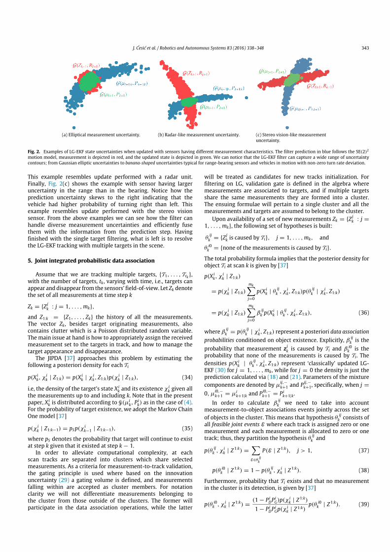
J. Ćesić et al. / Robotics and Autonomous Systems 83 (2016) 338–348 343
(a) Elliptical measurement uncertainty. (b) Radar-like measurement uncertainty. (c) Stereo vision-like measurementuncertainty.
Fig. 2. Examples of LG-EKF state uncertainties when updated with sensors having different measurement characteristics. The filter prediction in blue follows the SE(2)2motion model, measurement is depicted in red, and the updated state is depicted in green. We can notice that the LG-EKF filter can capture a wide range of uncertaintycontours; from Gaussian elliptic uncertainties to banana-shaped uncertainties typical for range-bearing sensors and vehicles in motion with non-zero turn rate deviation.
This example resembles update performed with a radar unit.Finally, Fig. 2(c) shows the example with sensor having largeruncertainty in the range than in the bearing. Notice how theprediction uncertainty skews to the right indicating that thevehicle had higher probability of turning right than left. Thisexample resembles update performed with the stereo visionsensor. From the above examples we can see how the filter canhandle diverse measurement uncertainties and efficiently fusethem with the information from the prediction step. Havingfinished with the single target filtering, what is left is to resolvethe LG-EKF tracking with multiple targets in the scene.
5. Joint integrated probabilistic data association
Assume that we are tracking multiple targets, T1, . . . , Ttk,with the number of targets, tk, varying with time, i.e., targets canappear and disappear from the sensors’ field-of-view. Let Zk denotethe set of all measurements at time step k
Zk = Z jk : j = 1, . . . ,mk,
and Z1:k = Z1, . . . , Zk the history of all the measurements.The vector Zk, besides target originating measurements, alsocontains clutter which is a Poisson distributed random variable.The main issue at hand is how to appropriately assign the receivedmeasurement set to the targets in track, and how to manage thetarget appearance and disappearance.
The JIPDA [37] approaches this problem by estimating thefollowing a posteriori density for each Ti
p(X ik, χ
ik | Z1:k) = p(X i
k | χ ik, Z1:k)p(χ
ik | Z1:k), (34)
i.e, the density of the target’s state X ik and its existence χ i
k given allthe measurements up to and including k. Note that in the presentpaper, X i
k is distributed according to G(µik, P
ik) as in the case of (4).
For the probability of target existence, we adopt the Markov ChainOne model [37]
p(χ ik | Z1:k−1) = pSp(χ i
k−1 | Z1:k−1), (35)
where pS denotes the probability that target will continue to existat step k given that it existed at step k − 1.
In order to alleviate computational complexity, at eachscan tracks are separated into clusters which share selectedmeasurements. As a criteria for measurement-to-track validation,the gating principle is used where based on the innovationuncertainty (29) a gating volume is defined, and measurementsfalling within are accepted as cluster members. For notationclarity we will not differentiate measurements belonging tothe cluster from those outside of the clusters. The former willparticipate in the data association operations, while the latter
will be treated as candidates for new tracks initialization. Forfiltering on LG, validation gate is defined in the algebra wheremeasurements are associated to targets, and if multiple targetsshare the same measurements they are formed into a cluster.The ensuing formulae will pertain to a single cluster and all themeasurements and targets are assumed to belong to the cluster.
Upon availability of a set of new measurements Zk = Z jk : j =
1, . . . ,mk, the following set of hypotheses is built:
θijk = Z j
k is caused by Ti, j = 1, . . . ,mk, and
θ i0k = none of the measurements is caused by Ti.
The total probability formula implies that the posterior density forobject Ti at scan k is given by [37]
p(X ik, χ
ik | Z1:k)
= p(χ ik | Z1:k)
mkj=0
p(X ik | θ
ijk , χ i
k, Z1:k)p(θijk | χ i
k, Z1:k)
= p(χ ik | Z1:k)
mkj=0
βijk p(X
ik | θ
ijk , χ i
k, Z1:k), (36)
where βijk = p(θ ij
k | χ ik, Z1:k) represent a posteriori data association
probabilities conditioned on object existence. Explicitly, β ijk is the
probability that measurement z jk is caused by Ti and β i0k is the
probability that none of the measurements is caused by Ti. Thedensities p(X i
k | θijk , χ i
k, Z1:k) represent ‘classically’ updated LG-EKF (30) for j = 1, . . . ,mk, while for j = 0 the density is just theprediction calculated via (18) and (21). Parameters of the mixturecomponents are denoted by µ
ij,−k+1 and P ij,−
k+1, specifically, when j =
0, µi0,−k+1 = µi
k+1|k and P i0,−k+1 = P i
k+1|k.In order to calculate β
ijk we need to take into account
measurement-to-object associations events jointly across the setof objects in the cluster. This means that hypothesis θ
ijk consists of
all feasible joint events E where each track is assigned zero or onemeasurement and each measurement is allocated to zero or onetrack; thus, they partition the hypothesis θ
ijk and
p(θ ijk , χ i
k | Z1:k) =
E∈θ
ijk
P(E | Z1:k), j > 1, (37)
p(θ i0k | Z1:k) = 1 − p(θ ij
k , χ ik | Z1:k). (38)
Furthermore, probability that Ti exists and that no measurementin the cluster is its detection, is given by [37]
p(θ i0k , χ i
k | Z1:k) =(1 − P i
DPiG)p(χ
ik | Z1:k)
1 − P iDP
iGp(χ
ik | Z1:k)
p(θ i0k | Z1:k). (39)

344 J. Ćesić et al. / Robotics and Autonomous Systems 83 (2016) 338–348
To calculate P(E | Z1:k), for each joint event E we define:set of targets allocated no measurement, T0(E), and set of tracksallocated one measurement, T1(E). Following [37,38] we obtain
P(E | Z1:k) = C−1k
i∈T0(E)
(1 − P iDP
iGP(χ i
k | Z1:k−1))
·
i∈T1(E)
P iDP
iGP(χ i
k | Z1:k−1)pik(τ (E, i))ρk(τ (E, i))
, (40)
where P id is the probability ofTi being detected, P i
G is the probabilitythat the correct measurement will be inside the validation gate ofTi, τ (E, i) is the index of measurement allocated to Ti under jointevent E, ρk(τ (E, i)) denotes a priori clutter measurement densityat zτ(E,i)
k , and C−1k is the normalization constant calculated from the
fact that E are mutually exclusive and form an exhaustive set, i.e.,E P(E | Z1:k) = 1. The innovation is calculated by using results
from (29)
pik(τ (E, i)) =1PG
pik(ντ(E,i)k ; 0, Hk+1Pk+1|kH
Tk+1 + Rk+1). (41)
The innovation in (41) is normalized by PG in order to account forthe validation gating, i.e., since it is truncated to integrate to unity.Finally, we have all the elements to determine the probability oftarget existence
p(χ ik | Z1:k) =
mkj=0
p(θ ijk , χ i
k | Z1:k), (42)
and to calculate the data association probabilities
βijk =
p(θ ijk , χ i
k | Z1:k)
p(χ ik | Z1:k)
, j = 0, . . . ,mk. (43)
Note that all the operations concerning a specific target Ti,described so far in the section, are carried out in the pertainingalgebra of µi
k+1|k, since, we are still at the update stage of the LG-EKF. To calculate the final a posteriori state estimate the JIPDA logicdictates reducing the mixture in (36) to a single density with thefollowing parameters [50,38]
µi,−k+1 =
mkj=0
βijk µ
ij,−k+1, (44)
P i,−k+1 =
mkj=0
(P ij,−k+1 + µ
ij,−k+1(µ
ij,−k+1)
T) − µi,−k+1(µ
i,−k+1)
T. (45)
As in the case of the LG-EKF update, E[ϵ−
k+1] = µi,−k+1 = 0p×1; thus,
before mapping the updated state and covariance to G we have toperform reparametrization [40]
µik+1 = µi
k+1|k expG
[µ
i,−k+1]
∧
G
P ik+1 = ΦG(µ
i,−k+1)P
i,−k+1ΦG(µ
i,−k+1)
T.
(46)
6. Experimental results
6.1. System overview
The experiments were carried out using two radar units anda stereo camera system, mounted on a sensor platform on top ofa vehicle. The sensor platform was constructed so that the stereocamera is placed in-between the two radar units as shown in Fig. 1.
In the present paper we used the Continental Short RangeRadar 209–2 units (measurement range of 50 m) configured tooperate in the cluster mode, at a rate of 15 Hz. The field of view
is 150° horizontally and 12° vertically, with the resolution in thehorizontal direction of 1°, while there is no discrimination of theangle in vertical direction, and hence the radar cluster data canbe considered as 2D measurements. After each scanning cycle theradar can deliver a cluster consisting of up to 128 detections. Inthe prefiltering stage we dismissed all the cluster measurementswhose radar cross section, i.e., the measure of the reflectivestrength, did not exceed −5 dBm.
The stereo images were recorded with the monochrome PointGrey Bumblebee XB3 camera system. This system is a 3-sensormulti-baseline stereo camera with 1.3 mega-pixel global shuttersensors. The image resolution is 1280×960 pixels, with horizontalfield of view of 66°. The experiments were carried out at themaximum frame rate of 16 Hz, and by using the largest, 24 cmlong baseline, since the expected target measurement range is upto 50m. The stereo image synchronizationwas executed internally,while the experiment was recorded in the auto-exposure mode ofthe camera.
Given that the sensors are closely spaced, mechanically alignedusing custom-made plates on the same rail, and since we performsensor fusion at the state level, the inter-sensor calibration wasdone by measuring the mounting position displacements by hand.Moreover, due to the coarse nature of radar measurements wefind the current rail-mounting sufficiently precise to assert thatdifferences in the orientation of the sensor coordinate framescan be neglected for case of the present sensor setup. However,for arbitrary radar and stereo vision setups a closer inspectionof the calibration problem might be required [7]. Furthermore,special attention was taken to assure the clock synchronization,since our approach relies on state estimation performed in anasynchronous manner. Although both sensors work at closefrequencies, generally this might not be the case, and the approachof asynchronous filtering is kept for the sake of generality. Theprediction step directly depends on the time period T , i.e., the timepassed between the two consecutive steps k and k + 1. Therefore,a clock drift or large delay in data acquisition could significantlyaffect the performance of the algorithm.
6.2. Stereo detection procedure
The main goal of the stereo image processing part of thealgorithm is to detect moving objects in the scene, while themotion of the observer makes this task especially challenging.However, this work focuses on the estimation procedure andthe fusion of two sensor modalities, hence the sole stereo baseddetection of moving objects is only briefly described.
The first part of the algorithm works on the ego-motionestimation, which results in transformation matrix between theprevious and the current camera frame. Regarding this issue,we employed our SOFT algorithm [24], which has proven to bevery robust on the appearance of moving objects in the scene,illumination changes, various specularities, sensor overexposureetc. However, SOFT uses very sparse set of salient feature points,which are not sufficient to reliably detect objects in the scene.Therefore, we employ the corner detector from [51] for detectionof semi-dense set of feature points. Position and velocity of eachdetected feature is estimated in 3D Euclidean space. Now we needto determine the correspondences between features in the leftand the right image of the current and previous frame. For thispurposewehave used the optical flowprocedure presented in [52],and have computed the correspondences by using the stereo blockmatching algorithm from [53].
Since the images are rectified, all the feature points fromthe previous frame are projected into 3D world frame througha standard pinhole camera model, and then are back-projectedinto the current camera frame by compounding the position with

J. Ćesić et al. / Robotics and Autonomous Systems 83 (2016) 338–348 345
the motion matrix obtained from the ego-motion algorithm. Suchtransformed 3D points from the previous frame connected tocorresponding 3D points from the current frame form a vectorfield, with each vector representing a motion of corresponding3D point relative to the world frame. Since the measurementuncertainties are highly anisotropic in 3D space, it is difficult toaccurately determine the motion intensity along the optical axisdirection. Hence, we project the vectors into the image planewhere the uncertainties are more evenly distributed, and applythe threshold on the magnitude of motion of each point. Theremaining vectors are then connected into clusters by respectingboth translational and rotational parameters. Finally, we considereach clusters corresponds to a moving object if at least 3 vectorsappear within it, and describe it with the centroid point of all thecorresponding points. The positions of themoving objects detectedwith the stereo camera system are finally projected into the radarplane and passed to the multitarget tracking algorithm presentedin Section 5.
The projection of raw detections of the stereo vision baseddetection (red circles) and radar readings (green circles) onto theimage plane along with filter tracks (yellow circles) is shown inFig. 3. The images represent four snapshots of the experimentwhich illustrates the drawbacks of using just a single sensingtechnology. For example, in the top-most snapshotwithin Fig. 3 theradar did not capture the twomotorcycles, while the stereo cameramanaged to detect their motion. The second snapshot gives anexample of a busy intersection, while the third snapshot shows anexamplewhere the vehicle right in front of the ego-vehiclewas notdetected by the stereo camera due to moving along the camera’soptical axis whereas the radar provided consistent detections andthe vehicle was tracked by the filter. The final snapshot shows anexample where the radar did not detect a vehicle and a pedestrian,while the stereo camera managed to consistently detect theirmotion and respective filter tracks were obtained.
6.3. Real-world experiments
The experiments were conducted with the sensor platformequipped vehicle driving through an urban environment. Thealgorithm was tested in several highly dynamic scenarios,involving cars, trams and pedestrians. The process noise intensitiesfor the asynchronous filter were set to qx = qy = 1 andqω = (2 π
180 )2. The clutter size and the probability of detection
were set to cradar = 10 and P radarD = 0.7, respectively. The
radar unit likelihood was configured such that the measurementuncertainty in the bearing component wasmφ,radar
k+1 ∼ NR1(0, 2°2),while the measurement uncertainty in the range component wasmr,radar
k+1 ∼ NR1(0, 0.252). The clutter size related to the stereovision systemwas set to cstereo = 2, while the detection probabilitywas P stereo
D = 0.75. The stereo vision likelihood was configured sothat the measurement uncertainty in the bearing component wasmφ,stereo
k+1 ∼ NR1(0, 0.5°2), while the measurement uncertainty inthe range component was mr,stereo
k+1 ∼ NR1(0, 12). The JIPDA filtergating probability was PG = 0.9, and the survival probability waspS = 0.95. We have implemented an approach where the tracksare confirmed to be truly existing objects once the probability ofobject existence exceeded the value of p(χ i
k | Z1:k) = 0.9. Thetracks were deleted once the probability of existence fell belowp(χ i
k | Z1:k) = 0.1.The first experiment, lasting about 60 s, involved a scenario in
which the vehicle turned right and kept driving down an avenue.The results of this experiment are shown in Fig. 4. In this exampleit is important to note the very dense traffic on the left-handside of the vehicle during the turn, which represents a very busyintersection (see themost bottom image in Fig. 3). However, due to
Fig. 3. Four snapshots of experiments illustrating detections of the stereo camera(red circles) and radar readings (green circles), which serve as the input for thetracking algorithm (yellow circles). The red lines depict optical flow vectors ofthe detected motion. An accompanying video is available at https://youtu.be/Br-qwez1L18. (For interpretation of the references to color in this figure legend, thereader is referred to the web version of this article.)
high radar clutter, it occasionally happened that the clutter causedfalse tracks. Such an example can be seen on the right-hand imageof Fig. 4. Even though the algorithm manages to track the vehicleson the road (in both directions), some objects, like the roadsidehedges next to the road and the pertaining radar clutter, havecaused the algorithm to detect them too as true targets. In thisexperiment, after raw sensor data preprocessing, on average therewere 6.46 radar detections and 1.69 stereo camera detections perframe which yielded 3560 filter initializations and 228 confirmedtracks.
In the second experiment, lasting about 85 s, the vehicledrove in one direction along a three lane avenue, performeda u-turn (at the same busy intersection as in Fig. 4) and keptdriving forward. The results of this experiment are shown inFig. 5. The dataset was collected on a three lane road, wherethe vehicle drove in the middle lane, and detected vehicles inboth the left and right lane. It can be noticed that again someradar measurements have caused the algorithm to believe thatroadside objects corresponds to true targets. By analyzing the
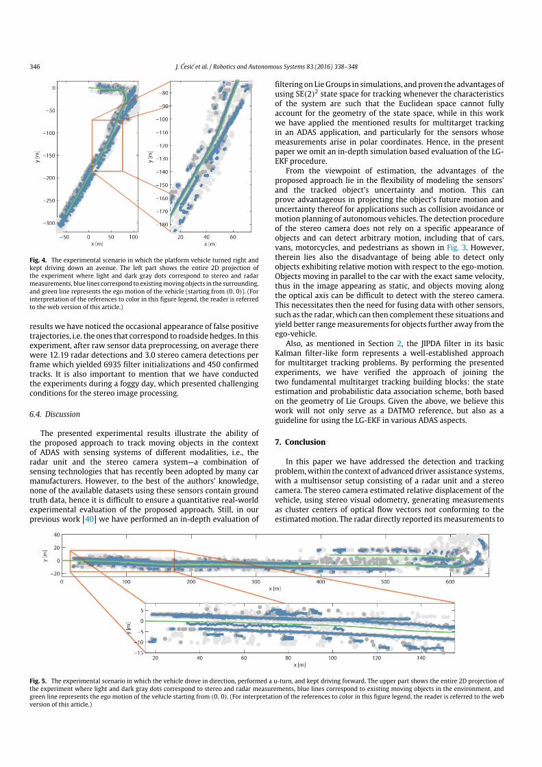
346 J. Ćesić et al. / Robotics and Autonomous Systems 83 (2016) 338–348
Fig. 4. The experimental scenario in which the platform vehicle turned right andkept driving down an avenue. The left part shows the entire 2D projection ofthe experiment where light and dark gray dots correspond to stereo and radarmeasurements, blue lines correspond to existingmoving objects in the surrounding,and green line represents the ego motion of the vehicle (starting from (0, 0)). (Forinterpretation of the references to color in this figure legend, the reader is referredto the web version of this article.)
results we have noticed the occasional appearance of false positivetrajectories, i.e. the ones that correspond to roadside hedges. In thisexperiment, after raw sensor data preprocessing, on average therewere 12.19 radar detections and 3.0 stereo camera detections perframe which yielded 6935 filter initializations and 450 confirmedtracks. It is also important to mention that we have conductedthe experiments during a foggy day, which presented challengingconditions for the stereo image processing.
6.4. Discussion
The presented experimental results illustrate the ability ofthe proposed approach to track moving objects in the contextof ADAS with sensing systems of different modalities, i.e., theradar unit and the stereo camera system—a combination ofsensing technologies that has recently been adopted by many carmanufacturers. However, to the best of the authors’ knowledge,none of the available datasets using these sensors contain groundtruth data, hence it is difficult to ensure a quantitative real-worldexperimental evaluation of the proposed approach. Still, in ourprevious work [40] we have performed an in-depth evaluation of
filtering on LieGroups in simulations, andproven the advantages ofusing SE(2)2 state space for tracking whenever the characteristicsof the system are such that the Euclidean space cannot fullyaccount for the geometry of the state space, while in this workwe have applied the mentioned results for multitarget trackingin an ADAS application, and particularly for the sensors whosemeasurements arise in polar coordinates. Hence, in the presentpaper we omit an in-depth simulation based evaluation of the LG-EKF procedure.
From the viewpoint of estimation, the advantages of theproposed approach lie in the flexibility of modeling the sensors’and the tracked object’s uncertainty and motion. This canprove advantageous in projecting the object’s future motion anduncertainty thereof for applications such as collision avoidance ormotion planning of autonomous vehicles. The detection procedureof the stereo camera does not rely on a specific appearance ofobjects and can detect arbitrary motion, including that of cars,vans, motorcycles, and pedestrians as shown in Fig. 3. However,therein lies also the disadvantage of being able to detect onlyobjects exhibiting relative motion with respect to the ego-motion.Objects moving in parallel to the car with the exact same velocity,thus in the image appearing as static, and objects moving alongthe optical axis can be difficult to detect with the stereo camera.This necessitates then the need for fusing data with other sensors,such as the radar, which can then complement these situations andyield better rangemeasurements for objects further away from theego-vehicle.
Also, as mentioned in Section 2, the JIPDA filter in its basicKalman filter-like form represents a well-established approachfor multitarget tracking problems. By performing the presentedexperiments, we have verified the approach of joining thetwo fundamental multitarget tracking building blocks: the stateestimation and probabilistic data association scheme, both basedon the geometry of Lie Groups. Given the above, we believe thiswork will not only serve as a DATMO reference, but also as aguideline for using the LG-EKF in various ADAS aspects.
7. Conclusion
In this paper we have addressed the detection and trackingproblem,within the context of advanced driver assistance systems,with a multisensor setup consisting of a radar unit and a stereocamera. The stereo camera estimated relative displacement of thevehicle, using stereo visual odometry, generating measurementsas cluster centers of optical flow vectors not conforming to theestimatedmotion. The radar directly reported itsmeasurements to
Fig. 5. The experimental scenario in which the vehicle drove in direction, performed a u-turn, and kept driving forward. The upper part shows the entire 2D projection ofthe experiment where light and dark gray dots correspond to stereo and radar measurements, blue lines correspond to existing moving objects in the environment, andgreen line represents the ego motion of the vehicle starting from (0, 0). (For interpretation of the references to color in this figure legend, the reader is referred to the webversion of this article.)
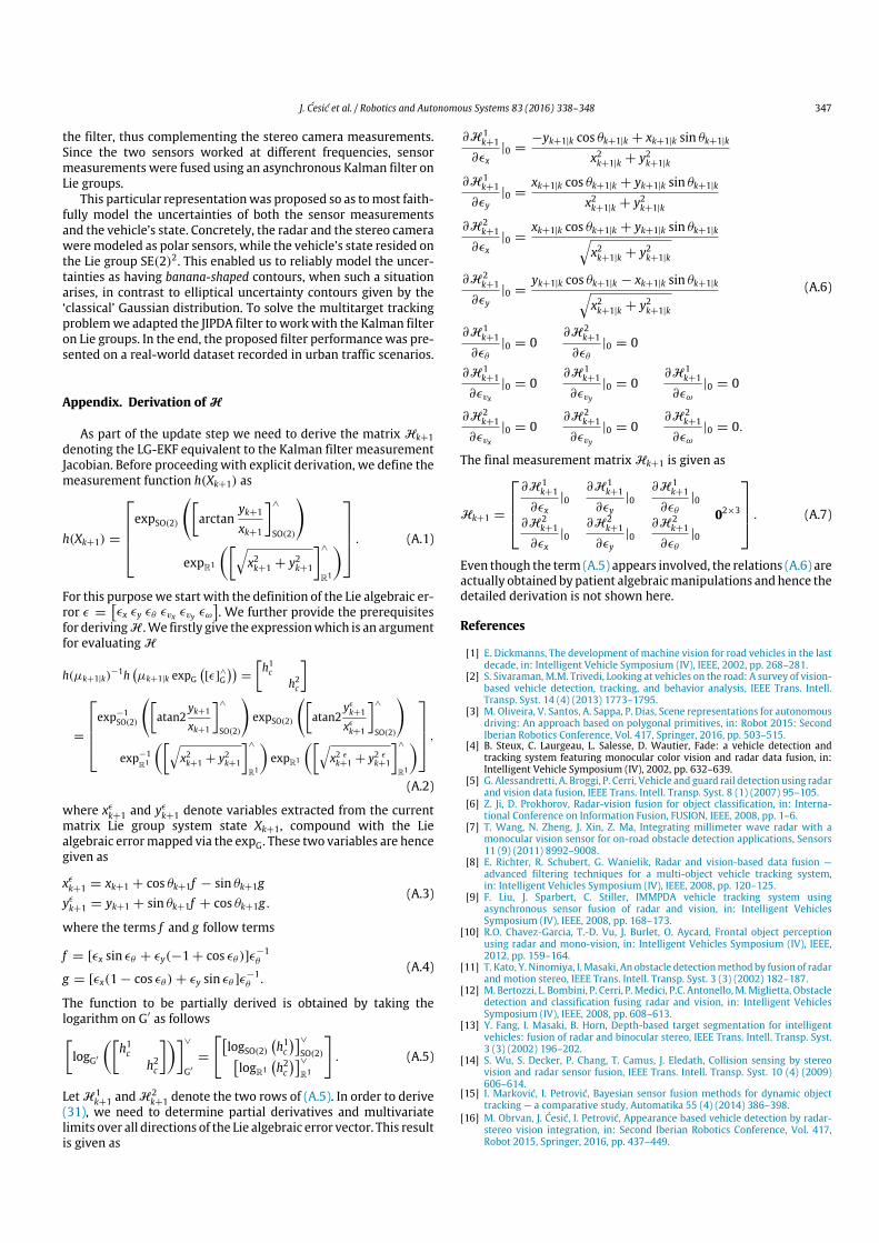
J. Ćesić et al. / Robotics and Autonomous Systems 83 (2016) 338–348 347
the filter, thus complementing the stereo camera measurements.Since the two sensors worked at different frequencies, sensormeasurements were fused using an asynchronous Kalman filter onLie groups.
This particular representationwas proposed so as tomost faith-fully model the uncertainties of both the sensor measurementsand the vehicle’s state. Concretely, the radar and the stereo cameraweremodeled as polar sensors, while the vehicle’s state resided onthe Lie group SE(2)2. This enabled us to reliably model the uncer-tainties as having banana-shaped contours, when such a situationarises, in contrast to elliptical uncertainty contours given by the‘classical’ Gaussian distribution. To solve the multitarget trackingproblemwe adapted the JIPDA filter to workwith the Kalman filteron Lie groups. In the end, the proposed filter performancewas pre-sented on a real-world dataset recorded in urban traffic scenarios.
Appendix. Derivation of H
As part of the update step we need to derive the matrix Hk+1denoting the LG-EKF equivalent to the Kalman filter measurementJacobian. Before proceeding with explicit derivation, we define themeasurement function h(Xk+1) as
h(Xk+1) =
expSO(2)
arctan
yk+1
xk+1
∧
SO(2)
expR1
x2k+1 + y2k+1
∧
R1
. (A.1)
For this purposewe start with the definition of the Lie algebraic er-ror ϵ =
ϵx ϵy ϵθ ϵvx ϵvy ϵω
. We further provide the prerequisites
for derivingH .We firstly give the expressionwhich is an argumentfor evaluating H
h(µk+1|k)−1h
µk+1|k expG
[ϵ]∧G
=
h1c
h2c
=
exp−1
SO(2)
atan2
yk+1
xk+1
∧
SO(2)
expSO(2)
atan2
yϵk+1
xϵk+1
∧
SO(2)
exp−1R1
x2k+1 + y2k+1
∧
R1
expR1
x2 ϵk+1 + y2 ϵ
k+1
∧
R1
,
(A.2)
where xϵk+1 and yϵ
k+1 denote variables extracted from the currentmatrix Lie group system state Xk+1, compound with the Liealgebraic errormapped via the expG. These two variables are hencegiven as
xϵk+1 = xk+1 + cos θk+1f − sin θk+1gyϵk+1 = yk+1 + sin θk+1f + cos θk+1g.
(A.3)
where the terms f and g follow terms
f = [ϵx sin ϵθ + ϵy(−1 + cos ϵθ )]ϵ−1θ
g = [ϵx(1 − cos ϵθ ) + ϵy sin ϵθ ]ϵ−1θ .
(A.4)
The function to be partially derived is obtained by taking thelogarithm on G′ as followslogG′
h1c
h2c
∨
G′
=
logSO(2)
h1c
∨SO(2)
logR1h2c
∨R1
. (A.5)
Let H1k+1 and H2
k+1 denote the two rows of (A.5). In order to derive(31), we need to determine partial derivatives and multivariatelimits over all directions of the Lie algebraic error vector. This resultis given as
∂H1k+1
∂ϵx|0 =
−yk+1|k cos θk+1|k + xk+1|k sin θk+1|k
x2k+1|k + y2k+1|k
∂H1k+1
∂ϵy|0 =
xk+1|k cos θk+1|k + yk+1|k sin θk+1|k
x2k+1|k + y2k+1|k
∂H2k+1
∂ϵx|0 =
xk+1|k cos θk+1|k + yk+1|k sin θk+1|kx2k+1|k + y2k+1|k
∂H2k+1
∂ϵy|0 =
yk+1|k cos θk+1|k − xk+1|k sin θk+1|kx2k+1|k + y2k+1|k
∂H1k+1
∂ϵθ
|0 = 0∂H2
k+1
∂ϵθ
|0 = 0
∂H1k+1
∂ϵvx
|0 = 0∂H1
k+1
∂ϵvy
|0 = 0∂H1
k+1
∂ϵω
|0 = 0
∂H2k+1
∂ϵvx
|0 = 0∂H2
k+1
∂ϵvy
|0 = 0∂H2
k+1
∂ϵω
|0 = 0.
(A.6)
The final measurement matrix Hk+1 is given as
Hk+1 =
∂H1
k+1
∂ϵx|0
∂H1k+1
∂ϵy|0
∂H1k+1
∂ϵθ
|0
∂H2k+1
∂ϵx|0
∂H2k+1
∂ϵy|0
∂H2k+1
∂ϵθ
|0
02×3
. (A.7)
Even though the term (A.5) appears involved, the relations (A.6) areactually obtained bypatient algebraicmanipulations andhence thedetailed derivation is not shown here.
References
[1] E. Dickmanns, The development of machine vision for road vehicles in the lastdecade, in: Intelligent Vehicle Symposium (IV), IEEE, 2002, pp. 268–281.
[2] S. Sivaraman,M.M. Trivedi, Looking at vehicles on the road: A survey of vision-based vehicle detection, tracking, and behavior analysis, IEEE Trans. Intell.Transp. Syst. 14 (4) (2013) 1773–1795.
[3] M. Oliveira, V. Santos, A. Sappa, P. Dias, Scene representations for autonomousdriving: An approach based on polygonal primitives, in: Robot 2015: SecondIberian Robotics Conference, Vol. 417, Springer, 2016, pp. 503–515.
[4] B. Steux, C. Laurgeau, L. Salesse, D. Wautier, Fade: a vehicle detection andtracking system featuring monocular color vision and radar data fusion, in:Intelligent Vehicle Symposium (IV), 2002, pp. 632–639.
[5] G. Alessandretti, A. Broggi, P. Cerri, Vehicle and guard rail detection using radarand vision data fusion, IEEE Trans. Intell. Transp. Syst. 8 (1) (2007) 95–105.
[6] Z. Ji, D. Prokhorov, Radar-vision fusion for object classification, in: Interna-tional Conference on Information Fusion, FUSION, IEEE, 2008, pp. 1–6.
[7] T. Wang, N. Zheng, J. Xin, Z. Ma, Integrating millimeter wave radar with amonocular vision sensor for on-road obstacle detection applications, Sensors11 (9) (2011) 8992–9008.
[8] E. Richter, R. Schubert, G. Wanielik, Radar and vision-based data fusion —advanced filtering techniques for a multi-object vehicle tracking system,in: Intelligent Vehicles Symposium (IV), IEEE, 2008, pp. 120–125.
[9] F. Liu, J. Sparbert, C. Stiller, IMMPDA vehicle tracking system usingasynchronous sensor fusion of radar and vision, in: Intelligent VehiclesSymposium (IV), IEEE, 2008, pp. 168–173.
[10] R.O. Chavez-Garcia, T.-D. Vu, J. Burlet, O. Aycard, Frontal object perceptionusing radar and mono-vision, in: Intelligent Vehicles Symposium (IV), IEEE,2012, pp. 159–164.
[11] T. Kato, Y. Ninomiya, I.Masaki, An obstacle detectionmethod by fusion of radarand motion stereo, IEEE Trans. Intell. Transp. Syst. 3 (3) (2002) 182–187.
[12] M. Bertozzi, L. Bombini, P. Cerri, P.Medici, P.C. Antonello,M.Miglietta, Obstacledetection and classification fusing radar and vision, in: Intelligent VehiclesSymposium (IV), IEEE, 2008, pp. 608–613.
[13] Y. Fang, I. Masaki, B. Horn, Depth-based target segmentation for intelligentvehicles: fusion of radar and binocular stereo, IEEE Trans. Intell. Transp. Syst.3 (3) (2002) 196–202.
[14] S. Wu, S. Decker, P. Chang, T. Camus, J. Eledath, Collision sensing by stereovision and radar sensor fusion, IEEE Trans. Intell. Transp. Syst. 10 (4) (2009)606–614.
[15] I. Marković, I. Petrović, Bayesian sensor fusion methods for dynamic objecttracking — a comparative study, Automatika 55 (4) (2014) 386–398.
[16] M. Obrvan, J. Ćesić, I. Petrović, Appearance based vehicle detection by radar-stereo vision integration, in: Second Iberian Robotics Conference, Vol. 417,Robot 2015, Springer, 2016, pp. 437–449.

348 J. Ćesić et al. / Robotics and Autonomous Systems 83 (2016) 338–348
[17] A. Broggi, A. Cappalunga, C. Caraffi, S. Cattani, S. Ghidoni, P. Grisleri, P.P. Porta,M. Posterli, P. Zani, TerraMax vision at the urban challenge 2007, IEEE Trans.Intell. Transp. Syst. 11 (1) (2010) 194–205.
[18] B. Lefaudeux, F. Nashashibi, Real-time visual perception: Detection andlocalisation of static and moving objects from a moving stereo rig, in:Intelligent Transportation Systems Conference, ITSC, 2012, pp. 522–527.
[19] P. Lenz, J. Ziegler, A. Geiger, M. Roser, Sparse scene flow segmentationfor moving object detection in urban environments, in: Intelligent VehiclesSymposium (IV), 2011, pp. 926–932.
[20] A. Wedel, T. Brox, T. Vaudrey, C. Rabe, U. Franke, D. Cremers, Stereoscopicscene flow computation for 3D motion understanding, Int. J. Comput. Vis. 95(1) (2011) 29–51.
[21] B. Barrois, S. Hristova, C.Wohler, F. Kummert, C. Hermes, 3D pose estimation ofvehicles using a stereo camera, in: Intelligent Vehicles Symposium (IV), 2009,pp. 267–272.
[22] E. Ohn-bar, S. Sivaraman,M. Trivedi, Partially occluded vehicle recognition andtracking in 3D, in: Intell. Veh. Symposium (IV), 2013, pp. 1350–1355.
[23] J. Almeida, V. Santos, Pedestrian pose estimation using stereo perception,in: Second Iberian Robotics Conference, Vol. 417, Robot 2015, Springer, 2016,pp. 491–502.
[24] I. Cvišić, I. Petrović, Stereo odometry based on careful feature selection andtracking, in: European Conference on Mobile Robots, ECMR, 2015.
[25] G. Bourmaud, R. Mégret, M. Arnaudon, A. Giremus, Continuous-discreteextended kalman filter on matrix lie groups using concentrated Gaussiandistributions, J. Math. Imaging Vision 51 (1) (2014) 209–228.
[26] R.P.S. Mahler, Multitarget Bayes filtering via first-order multitarget moments,IEEE Trans. Aerosp. Electron. Syst. 39 (4) (2003) 1152–1178.
[27] B.-N. Vo, S. Singh, A. Doucet, Sequential monte carlo methods for multi-targetfiltering with random finite sets, IEEE Trans. Aerosp. Electron. Syst. 41 (4)(2005) 1224–1245.
[28] B.-N. Vo,W.-K. Ma, The Gaussianmixture probability hypothesis density filter,IEEE Trans. Signal Process. 54 (11) (2006) 4091–4104.
[29] R. Mahler, PHD filters of higher order in target number, IEEE Trans. Aerosp.Electron. Syst. 43 (4) (2007) 1523–1543.
[30] B.-T. Vo, B.-N. Vo, A. Cantoni, Analytic implementations of the cardinalizedprobability hypothesis density filter, IEEE Trans. Signal Process. 55 (7) (2007)3553–3567.
[31] R. Mahler, Statistical Multisource-Multitarget Information Fusion, ArthechHouse, 2007.
[32] B.T. Vo, B.N. Vo, A. Cantoni, The cardinality balanced multi-target multi-Bernoulli filter and its implementations, IEEE Trans. Signal Process. 57 (2)(2009) 409–423.
[33] S. Reuter, B.T. Vo, B.N. Vo, K. Dietmayer, The labeledmulti-Bernoulli filter, IEEETrans. Signal Process. 62 (12) (2014) 3246–3260.
[34] H. Deusch, S. Reuter, K. Dietmayer, The labeled multi-Bernoulli SLAM filter,IEEE Signal Process. Lett. 22 (10) (2015) 1561–1565.
[35] D. Reid, An algorithm for tracking multiple targets, IEEE Trans. Automat.Control 24 (6) (1979) 843–854.
[36] Y. Bar-Shalom, E. Tse, Sonar tracking of multiple targets using jointprobabilistic data association filter, Automatica 11 (1975) 451–460.
[37] D. Mušicki, R. Evans, Joint integrated probabilistic data association — JIPDA,IEEE Trans. Aerosp. Electron. Syst. 40 (3) (2004) 1093–1099.
[38] S. Challa, M.R. Morelande, D. Mušicki, R.J. Evans, Fundamentals of objecttracking, 2011.
[39] J.L. Williams, Marginal multi-Bernoulli filters: RFS derivation of MHT, JIPDAand association-based MeMBer, IEEE Trans. Aerosp. Electron. Syst. 51 (3)(2015) 1664–1687.
[40] J. Ć, I. Marković, I. Petrović, Moving object tracking employing rigid bodydynamics on matrix Lie groups, in: Submitted to International Conference onInformation Fusion, FUSION, 2016.
[41] C. Hertzberg, R. Wagner, U. Frese, L. Schröder, Integrating generic sensorfusion algorithms with sound state representations through encapsulation ofmanifolds, Inf. Fusion 14 (1) (2013) 57–77.
[42] G.S. Chirikjian, StochasticModels, Information Theory, and Lie Groups, Volume2: Analytic Methods and Modern Applications, Springer, 2012.
[43] W. Park, Y. Wang, G.S. Chirikjian, The path-of-probability algorithm forsteering and feedback control of flexible needles, Int. J. Robot. Res. 29 (7)(2010) 813–830.
[44] T.D. Barfoot, P.T. Furgale, Associating uncertainty with three-dimensionalposes for use in estimationproblems, IEEE Trans. Robot. 30 (3) (2014) 679–693.
[45] Y. Wang, G.S. Chirikjian, Nonparametric second-order theory of errorpropagation on motion groups, Int. J. Robot. Res. 27 (11) (2008) 1258–1273.
[46] K.C.Wolfe,M.Mashner, G.S. Chirikjian, Bayesian fusion on Lie groups, J. Algebr.Stat. 2 (1) (2011) 75–97.
[47] Y. Bar-Shalom, T. Kirubarajan, X.-R. Li, Estimation with Applications toTracking and Navigation, John Wiley & Sons, Inc., 2002.
[48] S. Thrun, W. Burgard, D. Fox, Probabilistic Robotics, The MIT Press, 2006.[49] R. Schubert, C. Adam,M. Obst, N. Mattern, V. Leonhardt, G.Wanielik, Empirical
evaluation of vehicular models for ego motion estimation, in: IntelligentVehicles Symposium, IEEE, 2011, pp. 534–539.
[50] D. Salmond, Mixture reduction algorithms for point and extended objecttracking in clutter, IEEE Trans. Aerosp. Electron. Syst. 45 (2) (2009) 667–686.
[51] J. Shi, C. Tomasi, Good features to track, in: 1994 IEEE Computer SocietyConference on Computer Vision and Pattern Recognition, 1994. ProceedingsCVPR ’94, 1994, pp. 593–600.
[52] J.-Y. Bouguet, Pyramidal implementation of the Lucas Kanade feature trackerdescription of the algorithm, Tech. Rep. 2, Intel Corporation, MicrosoftResearch Labs, 2000.
[53] K. Konolige, Small vision systems: Hardware and implementation, in: RoboticsResearch, Springer, London, 1998, pp. 203–212.
Josip Ćesić has received his B.Sc. and M.Sc. degree (MagnaCum Laude) in electrical engineering and informationtechnology from University of Zagreb, Faculty of ElectricalEngineering and Computing (UNIZG-FER) in 2011 and2013, respectively. He finished part of his master studiesat Chalmers University of Technology, Sweden. He isemployed as a research assistant at the Department ofControl and Computer Engineering at FER Zagreb sinceApril 2013. During the undergraduate studies he receivedDean’s Award and Special Dean’s Award for outstandingachievements on the first year of studies and the overall
B.Sc. level, respectively. During the graduate studies he received Rector’s Awardand Special Rector’s Award for practical applications in the fields of robotics andcontrol systems. He was also awarded with Scholarship from the Croatian Ministryof Science, Scholarship of the University of Zagreb and Scholarship of the City ofZagreb. His main research interests are in the areas of autonomous systems andmobile robotics, estimation theory and sensor processing.
Ivan Marković received the B.Sc. and the Ph.D. degree inElectrical Engineering from the University of Zagreb, Fac-ulty of Electrical Engineering andComputing (FER), Croatiain 2008 and 2014, respectively. He is currently employedat the FER, Zagreb, as a Research and Teaching Assistantfunded by the Ministry of Science, Education and Sport,Republic of Croatia. During his undergraduate studies,for outstanding academic achievements, he received the‘‘Institute for Nuclear Technology Award’’ and the ‘‘JosipLončar Award’’ in 2007 and 2006, respectively. In 2013and 2014 he was a visiting researcher at Inria Rennes—
Bretagne Atlantique in the Lagadic group directed by Prof. François Chaumette,Ph.D. He also serves as the coordinator of the technical editing team of the Au-tomatika journal. Hismain research interests are inmobile robotics, estimation the-ory and human–robot interaction.
Igor Cvišić received diploma degree in Electrical Engineer-ing from the Faculty of Electrical Engineering and Comput-ing (FER Zagreb), University of Zagreb, Croatia in 2001. Heis currently employed at the FER, Department of Controland Computer Engineering, as a researcher on the EU FP7ACROSS project, and he is pursuing his Ph.D. degree. Previ-ously, he worked at DAMCO as an R&D Engineer, where hesuccessfully coordinated and developed more than 10 dif-ferent custom made industrial automated systems basedon manipulation guided by computer vision. His researchinterests include robotics vision, system control and au-
tomation, electronics and autonomous flying vehicles. For hiswork, hewas awardedwith the Best Student Paper Award at the RAADWorkshop 2013, Portorož, Slovenia.
Ivan Petrović received B.Sc. degree in 1983, M.Sc. degreein 1989 and Ph.D. degree in 1998, all in ElectricalEngineering from the Faculty of Electrical Engineering andComputing (FER Zagreb), University of Zagreb, Croatia. Hehad been employed as an R&D engineer at the Institute ofElectrical Engineering of the Končar Corporation in Zagrebfrom 1985 to 1994. Since 1994 he has been with FERZagreb, where he is currently a full professor. He teachesa number of undergraduate and graduate courses in thefield of control systems and mobile robotics. His researchinterests include various advanced control strategies and
their applications to control of complex systems and mobile robots navigation. Hehas published more than 40 journals and 160 conference papers, and results of hisresearch have been implemented in several industrial products. He is a member ofIEEE, IFAC – TC on Robotics and FIRA – Executive committee. He is a member of theCroatian Academy of Engineering and Editor-in-Chief of the Automatika journal.

126 publications
publication 8
J. Ćesić, I. Marković, and I. Petrović. Mixture Reduction on Matrix Lie Groups. IEEE Signal
Processing Letters, 24(11):1719–1723, 2017.

IEEE SIGNAL PROCESSING LETTERS, VOL. 24, NO. 11, NOVEMBER 2017 1719
Mixture Reduction on Matrix Lie GroupsJosip Cesic, Member, IEEE, Ivan Markovic, Member, IEEE, and Ivan Petrovic, Member, IEEE
Abstract—Many physical systems evolved on matrix Lie groupsand mixture filtering designed for such manifolds represent aninevitable tool for challenging estimation problems. However, mix-ture filtering faces the issue of a constantly growing number ofcomponents, hence requiring appropriate mixture reduction tech-niques. In this letter, we propose a mixture reduction approachfor distributions on matrix Lie groups, called the concentratedGaussian distributions (CGDs). This entails appropriate reparam-eterization of CGD parameters to compute the KL divergence,pick and merge the mixture components. Furthermore, we alsointroduce a multitarget tracking filter on Lie groups as a mixturefiltering study example for the proposed reduction method. In par-ticular, we implemented the probability hypothesis density filteron matrix Lie groups. We validate the filter performance usingthe optimal subpattern assignment metric on a synthetic datasetconsisting of 100 randomly generated multitarget scenarios.
Index Terms—Estimation on matrix lie groups, mixture reduc-tion, multitarget tracking, probability hypothesis density filter.
I. INTRODUCTION
MANY statistical and engineering problems require mod-eling of complex multimodal data, wherein mixture
distributions became an inevitable tool [1], [2], primarily intraditional application domains like radar and sonar tracking[3], and later in different modern fields such as computer vision[4], speech recognition [5], or multimedia processing [6]. Ap-proaches relying on mixture distributions often face the problemof large or an ever increasing number of mixture components;hence, the growth of components must be controlled by approx-imating the original mixture with a mixture of a reduced size[7]–[9]. For example, in the case of multitarget tracking ap-plications, by employing conventional Gaussian mixture basedfilters [10], [11], during the recursion process, the number ofcomponents inevitably increases. This appears first due to ap-pearance of newly birthed or spawned components, and second,due to inclusion of multiple measurements, which results in ageometrical increase in the number of components.
Another important aspect of estimation is the state space ge-ometry; hence, many works have been dedicated to appropriateuncertainty modeling and estimation techniques for a wide range
Manuscript received May 3, 2017; revised June 23, 2017; accepted July 2,2017. Date of publication July 5, 2017; date of current version October 11,2017. This work has been supported from the Unity Through KnowledgeFund (no. 24/15) under the project Cooperative Cloud based SimultaneousLocalization and Mapping in Dynamic Environments (cloudSLAM) and theEuropean Union’s Horizon 2020 research and innovation programme undergrant agreement No 688117 (SafeLog). The associate editor coordinating thereview of this manuscript and approving it for publication was Prof. MarcoFelipe Duarte. (Corresponding Author: Ivan Markovic.)
The authors are with the Faculty of Electrical Engineering and Comput-ing, University of Zagreb, Zagreb 10000, Croatia (e-mail: [email protected];[email protected]; [email protected]).
Digital Object Identifier 10.1109/LSP.2017.2723765
of applications [12]–[15], motivated by theoretical and imple-mentation difficulties caused by treating a constrained problemnaively with Euclidean tools. For example, Lie groups are nat-ural ambient (state) spaces for description of the dynamics ofrigid body mechanical systems. In [16], it has been observedthat the distribution of the pose of a differential drive mobilerobot is not a Gaussian distribution in Cartesian coordinates,but rather a distribution on the special Euclidean group SE(2).Similarly, in [17], it was discussed the uncertainty associationwith three-dimensional (3-D) pose employing the SE(3) group.Furthermore, attitude estimation arises naturally on the SO(3)group [15]. In [18], a feedback particle filter on matrix Liegroups was proposed, while in [19], [20], the authors proposedan extended Kalman filter on matrix Lie groups (LG-EKF),building the theory upon the concentrated Gaussian distribution(CGD) on matrix Lie groups [21].
In this letter, we address finite mixtures of distributions onmatrix Lie groups. We propose a novel approach to CGD mix-ture reduction, which required finding solutions for computingKullback–Leibler divergence of CGD components and CGDcomponent merging. Furthermore, since previous methods re-quire choosing the appropriate tangent space, we also providean extensive analysis on the choice thereof. As a study example,we use the proposed reduction method in a multitarget trackingscenario. We introduce the probability hypothesis density filter(PHD) on matrix Lie groups with approximation based on afinite mixture of CGDs.
II. MATHEMATICAL PRELIMINARIES
We now introduce theoretical preliminaries concerning Liegroups; however, for a more rigorous introduction, the reader isdirected to [22]. A Lie group G is a group that has the structureof a smooth manifold; moreover, a tangent space TX (G) is asso-ciated to X ∈ G such that the tangent space placed at the groupidentity, called Lie algebra g, is transferred by applying corre-sponding action to X . In this letter, we are interested in matrixLie groups that are usually the ones considered in engineeringand physical sciences.
The Lie algebra g ⊂ Rn×n associated to a p-dimensional ma-trix Lie group G ⊂ Rn×n is a p-dimensional vector space. Thematrix exponential expG and matrix logarithm logG establish alocal diffeomorphism between the two
expG : g → G and logG : G → g. (1)
Furthermore, a natural relation exists between g and theEuclidean space Rp given through a linear isomorphism
[·]∨G : g → Rp and [·]∧G : Rp → g. (2)
For x ∈ Rp and X ∈ G, we use the following notation [23]:
exp∧G(x) = expG([x]∧G) and log∨
G(X) = [logG(X)]∨G . (3)
1070-9908 © 2017 IEEE. Personal use is permitted, but republication/redistribution requires IEEE permission.See http://www.ieee.org/publications standards/publications/rights/index.html for more information.

1720 IEEE SIGNAL PROCESSING LETTERS, VOL. 24, NO. 11, NOVEMBER 2017
Lie groups are generally noncommutative, i.e., XY = Y X .However, the noncommutativity can be captured by the so-calledadjoint representation of G on g [24]
X exp∧G(y) = exp∧
G(AdG(X)y)X (4)
which can be seen as a way of representing the elements ofthe group as a linear transformation of the group’s algebra. Theadjoint representation of g, adG, is in fact the differential ofAdG at the identity. Another important result for working withLie group elements is the Baker–Campbell–Hausdorff (BCH)formula, which enables representing the product of Lie groupmembers as a sum in the Lie algebra. We will use the followingBCH formulae [24], [25]:
log∨G(exp∧
G(x) exp∧G(y)) = y + ϕG(y)x + O(||y||2) (5)
log∨G(exp∧
G(x + y) exp∧G(−x)) = ΦG(x)y + O(||y||2) (6)
where ϕG(y) =∑∞
n=0Bn adG(y )n
n ! , Bn are Bernoulli numbers,and ΦG(x) = ϕG(x)−1 . For many common groups used in en-gineering and physical sciences, closed-form expressions forϕG(·) and ΦG(·) can be found [17], [24]; otherwise, a truncatedseries expansion is used.
A. Concentrated Gaussian Distribution
Herein, we introduce the concept of the concentrated Gaus-sian distribution that is used to define random variables on matrixLie group. A random variable X ∈ G has a CGD with the meanμ and covariance Σ, i.e., X ∼ G(X;μ,Σ), if
X = exp∧G(ξ)μ (7)
where μ ∈ G, and ξ ∼ N (ξ;0p×1 ,Σ) is a zero-mean “classical”Gaussian random variable with the covariance Σ ⊂ Rp×p [17],[20]. Note that in this way, we are directly defining the CGDcovariance in the pertaining Lie algebra g, while the mean isdefined on the group G.
Given that the previous definition (7) then induces a proba-bility density function (pdf) of X over G as follows [17], [20]:
1 =
∫
Rp
1√(2π)p |Σ|
exp∧G
(− 1
2||ξ||2Σ
)dξ
=
∫
Gβ exp∧
G
(−1
2|| log∨
G(Xμ−1)||2Σ)
dX (8)
where ||x||2Σ = xTΣ−1x. Therein, the change of coordinates ξ =log∨
G(Xμ−1), with the pertaining differentials dX = |Φ(ξ)|dξ,resulted with the CGD normalizing constant
β = 1/√
(2π)p |Φ(log∨G(Xμ−1))ΣΦ(log∨
G(Xμ−1))T|. (9)
Note that this change of variables is valid if all eigenvaluesof Σ are small, i.e., almost all the mass of the distribution isconcentrated in a small neighborhood around the mean value[20]. The pdf over X is now fully determined by (8) and (9).
III. CGD MIXTURE REDUCTION
With the theoretical preliminaries setup, we continue withmixture reduction on matrix Lie groups. A finite mixture of ourpresent interest is given as the weighted sum of CGDs
N∑
i=1
wiG(X;μi,Σi) (10)
where wi are component weights and N is the total number ofmixture components. An illustration of (10) is given in Fig. 1.Component reduction procedures typically require three build-ing blocks: (i) component distance measure, (ii) componentpicking algorithm, and (iii) component merging. While vari-ous solutions exist for “classical” Gaussian mixtures [7]–[9],questions remain on how to approach the component numberreduction for CGD mixtures on matrix Lie groups. Therefore,first, we focus on the fundamental question of how to measurethe distance between two CGD components.
A. Component Distance Measure
Our aim is to use a standard information-theoretic measurebetween two CGD components, and we propose to use theKullback–Leibler (KL) divergence [26]. Let Gi = G(X;μi,Σi)and Gj = G(X;μj ,Σj ) be two mixture components with pi(X)and pj (X) as their respective pdfs. Since there is nothing intrin-sic in the definition of KL divergence that requires the underly-ing space to be Euclidean, by definition
DKL(Gi ,Gj ) =
∫
Gpi(X) log
(pi(X)
pj (X)
)dX . (11)
In order to evaluate the integral (11), we need to employ thechange of coordinates as in (8), but this time from the directionof the group G, i.e., from X ∈ G to ξ ∈ Rp . Note that in (8) thechange evolved around the distribution mean μ; however, sincein (11) generally μi = μj , we cannot apply the same approach.Hence, before evaluating (11), we first discuss how to changethe coordinates on the level of a single distribution.
Let G(X;μ,Σ) be a CGD, and if we change the coordinatesusing X = exp∧
G(ξ)μt , μt ∈ G, where μt = μ, we get
1 =
∫
Gβ exp∧
G
(−1
2|| log∨
G(Xμ−1)||2Σ)
dX
CoC≈∫
Rp
η exp∧G
(−1
2|| log∨
G(exp∧G(ξ)μtμ
−1)||2Σ)
dξ
(6)≈∫
Rp
η exp∧G
(−1
2||ΦG(rt)(ξ − rt)||2Σ
)dξ
=
∫
Rp
η exp∧G
(−1
2||ξ − rt ||2ϕG(rt )ΣϕT
G(rt )
)dξ (12)
where rt = log∧G(μμ−1
t ), η approximately evaluates to
η = β|Φ(ξ)| =|Φ(ξ)|√
(2π)p |Σ| · |Φ(log∨G(exp∧
G(ξ)μtμ−1))|
≈ 1√(2π)p |ϕG(rt)ΣϕG(rt)T|
(13)
and we obtain ξ ∼ N (ξ; rt , ϕG(rt)ΣϕTG(rt)).
Remark 1: Covariance of a CGD represents the uncertaintyrelevant only to the tangent space of its own mean. In [24], theauthors studied how the covariance changes if looked at fromthe perspective of a value that is different than the distributionmean. They dubbed this procedure “distribution unfolding.” Forexample, if we unfold G(X;μ,Σ) around an arbitrary μt ∈ G,using (5) and following [24], we get
ξt = log∨G
(exp∧
G(ξ)μμ−1t
)
≈ log∨G
(μμ−1
t
)+ ϕG
(log∨
G(μμ−1t )
)ξ . (14)
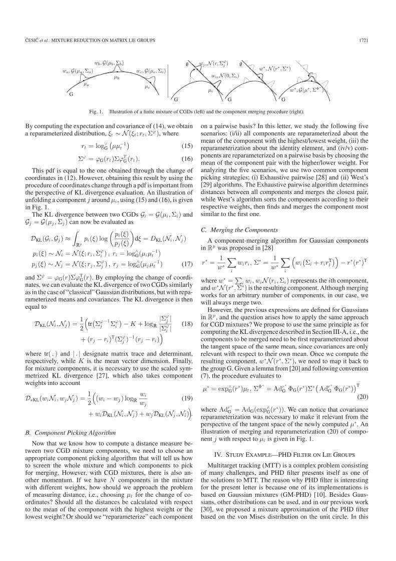
CESIC et al.: MIXTURE REDUCTION ON MATRIX LIE GROUPS 1721
Fig. 1. Illustration of a finite mixture of CGDs (left) and the component merging procedure (right).
By computing the expectation and covariance of (14), we obtaina reparameterized distribution, ξt ∼ N (ξt ; rt ,Σ
ϕ ), where
rt = log∨G
(μμ−1
t
)(15)
Σϕ = ϕG(rt)ΣϕTG (rt). (16)
This pdf is equal to the one obtained through the change ofcoordinates in (12). However, obtaining this result by using theprocedure of coordinates change through a pdf is important fromthe perspective of KL divergence evaluation. An illustration ofunfolding a component j around μi , using (15) and (16), is givenin Fig. 1.
The KL divergence between two CGDs Gi = G(μi,Σi) andGj = G(μj ,Σj ) can now be evaluated as
DKL(Gi ,Gj ) ≈∫
Rp
pi(ξ) log
(pi(ξ)
pj (ξ)
)dξ = DKL(Ni ,Nj )
pi(ξ) ∼ Ni = N (ξ; ri ,Σϕi ) , ri = log∧
G(μiμ−1t )
pj (ξ) ∼ Nj = N (ξ; rj ,Σϕj ) , rj = log∧
G(μjμ−1t ) (17)
and Σϕ = ϕG(r)ΣϕTG(r). By employing the change of coordi-
nates, we can evaluate the KL divergence of two CGDs similarlyas in the case of “classical” Gaussian distributions, but with repa-rameterized means and covariances. The KL divergence is thenequal to
DKL(Ni ,Nj ) =1
2
(tr(Σϕ
j−1
Σϕi
)− K + logR
|Σϕj |
|Σϕi | (18)
+ (rj − ri)T(Σϕ
j )−1(rj − ri))
where tr( . ) and | . | designate matrix trace and determinant,respectively, while K is the mean vector dimension. Finally,for mixture components, it is necessary to use the scaled sym-metrized KL divergence [27], which also takes componentweights into account
DsKL(wiNi , wjNj ) =1
2
((wi − wj ) logR
wi
wj(19)
+ wiDKL(Ni ,Nj ) + wjDKL(Nj ,Ni)).
B. Component Picking Algorithm
Now that we know how to compute a distance measure be-tween two CGD mixture components, we need to choose anappropriate component picking algorithm that will tell us howto screen the whole mixture and which components to pickfor merging. However, with CGD mixtures, there is also an-other momentum. If we have N components in the mixturewith different weights, how should we approach the problemof measuring distance, i.e., choosing μt for the change of co-ordinates? Should all the distances be calculated with respectto the mean of the component with the highest weight or thelowest weight? Or should we “reparameterize” each component
on a pairwise basis? In this letter, we study the following fivescenarios: (i/ii) all components are reparameterized about themean of the component with the highest/lowest weight, (iii) thereparameterization about the identity element, and (iv/v) com-ponents are reparameterized on a pairwise basis by choosing themean of the component pair with the higher/lower weight. Foranalyzing the five scenarios, we use two common componentpicking strategies; (i) Exhaustive pairwise [28] and (ii) West’s[29] algorithms. The Exhaustive pairwise algorithm determinesdistances between all components and merges the closest pair,while West’s algorithm sorts the components according to theirrespective weights, then finds and merges the component mostsimilar to the first one.
C. Merging the Components
A component-merging algorithm for Gaussian componentsin Rp was proposed in [28]
r∗ =1
w∗∑
i
wiri , Σ∗ =1
w∗∑
i
(wi
(Σi + rir
Ti
))− r∗(r∗)T
where w∗ =∑
i wi , wiN (ri,Σi) represents the ith component,and w∗N (r∗,Σ∗) is the resulting component. Although mergingworks for an arbitrary number of components, in our case, wewill always merge two.
However, the previous expressions are defined for Gaussiansin Rp , and the question arises how to apply the same approachfor CGD mixtures? We propose to use the same principle as forcomputing the KL divergence described in Section III-A, i.e., thecomponents to be merged need to be first reparameterized aboutthe tangent space of the same mean, since covariances are onlyrelevant with respect to their own mean. Once we compute theresulting component, w∗N (r∗,Σ∗), we need to map it back tothe group G. Given a lemma from [20] and following convention(7), the procedure evaluates to
μ∗ = exp∧G(r∗)μt, ΣΦ∗
= Adr ∗G ΦG(r∗)Σ∗( Adr ∗
G ΦG(r∗))T
(20)
where Adr ∗G = AdG(exp∧
G(r∗)). We can notice that covariancereparameterization was necessary to make it relevant from theperspective of the tangent space of the newly computed μ∗. Anillustration of merging and reparameterization (20) of compo-nent j with respect to μi is given in Fig. 1.
IV. STUDY EXAMPLE—PHD FILTER ON LIE GROUPS
Multitarget tracking (MTT) is a complex problem consistingof many challenges, and PHD filter presents itself as one ofthe solutions to MTT. The reason why PHD filter is interestingfor the present letter is because one of its implementations isbased on Gaussian mixtures (GM-PHD) [10]. Besides Gaus-sians, other distributions can be used, and in our previous work[30], we proposed a mixture approximation of the PHD filterbased on the von Mises distribution on the unit circle. In this
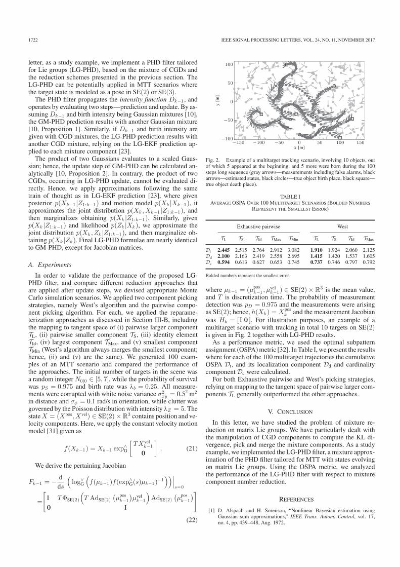
1722 IEEE SIGNAL PROCESSING LETTERS, VOL. 24, NO. 11, NOVEMBER 2017
letter, as a study example, we implement a PHD filter tailoredfor Lie groups (LG-PHD), based on the mixture of CGDs andthe reduction schemes presented in the previous section. TheLG-PHD can be potentially applied in MTT scenarios wherethe target state is modeled as a pose in SE(2) or SE(3).
The PHD filter propagates the intensity function Dk−1 , andoperates by evaluating two steps—prediction and update. By as-suming Dk−1 and birth intensity being Gaussian mixtures [10],the GM-PHD prediction results with another Gaussian mixture[10, Proposition 1]. Similarly, if Dk−1 and birth intensity aregiven with CGD mixtures, the LG-PHD prediction results withanother CGD mixture, relying on the LG-EKF prediction ap-plied to each mixture component [23].
The product of two Gaussians evaluates to a scaled Gaus-sian; hence, the update step of GM-PHD can be calculated an-alytically [10, Proposition 2]. In contrary, the product of twoCGDs, occurring in LG-PHD update, cannot be evaluated di-rectly. Hence, we apply approximations following the sametrain of thought as in LG-EKF prediction [23], where givenposterior p(Xk−1 |Z1:k−1) and motion model p(Xk |Xk−1), itapproximates the joint distribution p(Xk,Xk−1 |Z1:k−1), andthen marginalizes obtaining p(Xk |Z1:k−1). Similarly, givenp(Xk |Z1:k−1) and likelihood p(Zk |Xk ), we approximate thejoint distribution p(Xk,Zk |Z1:k−1), and then marginalize ob-taining p(Xk |Zk ). Final LG-PHD formulae are nearly identicalto GM-PHD, except for Jacobian matrices.
A. Experiments
In order to validate the performance of the proposed LG-PHD filter, and compare different reduction approaches thatare applied after update steps, we devised appropriate MonteCarlo simulation scenarios. We applied two component pickingstrategies, namely West’s algorithm and the pairwise compo-nent picking algorithm. For each, we applied the reparame-terization approaches as discussed in Section III-B, includingthe mapping to tangent space of (i) pairwise larger componentTL, (ii) pairwise smaller component TS, (iii) identity elementTId, (iv) largest component TMax, and (v) smallest componentTMin (West’s algorithm always merges the smallest component;hence, (ii) and (v) are the same). We generated 100 exam-ples of an MTT scenario and compared the performance ofthe approaches. The initial number of targets in the scene wasa random integer N0|0 ∈ [5, 7], while the probability of survivalwas pS = 0.975 and birth rate was λb = 0.25. All measure-ments were corrupted with white noise variance σ2
xy = 0.52 m2
in distance and σφ = 0.1 rad/s in orientation, while clutter wasgoverned by the Poisson distribution with intensity λZ = 5. Thestate X = (Xpos,Xvel) ∈ SE(2) × R3 contains position and ve-locity components. Here, we apply the constant velocity motionmodel [31] given as
f(Xk−1) = Xk−1 exp∧G
[TXvel
k−1
0
]. (21)
We derive the pertaining Jacobian
Fk−1 = − dds
(log∨
G
(f(μk−1)f(exp∧
G(s)μk−1)−1
))∣∣∣s=0
=
[I TΦSE(2)
(T AdSE(2)
(μpos
k−1
)μvel
k−1
)AdSE(2)
(μpos
k−1
)
0 I
]
(22)
Fig. 2. Example of a multitarget tracking scenario, involving 10 objects, outof which 5 appeared at the beginning, and 5 more were born during the 100steps long sequence (gray arrows—measurements including false alarms, blackarrows—estimated states, black circles—true object birth place, black square—true object death place).
TABLE IAVERAGE OSPA OVER 100 MULTITARGET SCENARIOS (BOLDED NUMBERS
REPRESENT THE SMALLEST ERROR)
Exhaustive pairwise West
TL TS TId TMax TMin TL TS TId TMax
Dt 2.445 2.515 2.764 2.912 3.082 1.910 1.924 2.060 2.125Dd 2.100 2.163 2.419 2.558 2.695 1.415 1.420 1.537 1.605Dc 0.594 0.613 0.627 0.653 0.745 0.737 0.746 0.797 0.792
Bolded numbers represent the smallest error.
where μk−1 = (μposk−1 , μ
velk−1) ∈ SE(2) × R3 is the mean value,
and T is discretization time. The probability of measurementdetection was pD = 0.975 and the measurements were arisingas SE(2); hence, h(Xk ) = Xpos
k and the measurement Jacobianwas Hk = [ I 0 ]. For illustration purposes, an example of amultitarget scenario with tracking in total 10 targets on SE(2)is given in Fig. 2 together with LG-PHD results.
As a performance metric, we used the optimal subpatternassignment (OSPA) metric [32]. In Table I, we present the resultswhere for each of the 100 multitarget trajectories the cumulativeOSPA Dt, and its localization component Dd and cardinalitycomponent Dc were calculated.
For both Exhaustive pairwise and West’s picking strategies,relying on mapping to the tangent space of pairwise larger com-ponents TL generally outperformed the other approaches.
V. CONCLUSION
In this letter, we have studied the problem of mixture re-duction on matrix Lie groups. We have particularly dealt withthe manipulation of CGD components to compute the KL di-vergence, pick and merge the mixture components. As a studyexample, we implemented the LG-PHD filter, a mixture approx-imation of the PHD filter tailored for MTT with states evolvingon matrix Lie groups. Using the OSPA metric, we analyzedthe performance of the LG-PHD filter with respect to mixturecomponent number reduction.
REFERENCES
[1] D. Alspach and H. Sorenson, “Nonlinear Bayesian estimation usingGaussian sum approximations,” IEEE Trans. Autom. Control, vol. 17,no. 4, pp. 439–448, Aug. 1972.

CESIC et al.: MIXTURE REDUCTION ON MATRIX LIE GROUPS 1723
[2] R. Chen and J. S. Liu, “Mixture Kalman filters,” J. Roy. Statist. Soc.:Series B (Statist. Methodol.), vol. 62, no. 3, pp. 493–508, 2000.
[3] S. S. Blackman, Multiple-Target Tracking with Radar Applications. Nor-wood, MA, USA: Artech House, 1986.
[4] C. Stauffer and W. E. L. Grimson, “Learning patterns of activity usingreal-time tracking,” IEEE Trans. Pattern Anal. Mach. Intell., vol. 22, no. 8,pp. 747–757, Aug. 2000.
[5] J. Goldberger and H. Aronowitz, “A distance measure between GMMsbased on the unscented transform and its application to speaker recogni-tion,” in Proc. Interspeech, 2005, pp. 1985–1989.
[6] A. Nikseresht and M. Gelgon, “Gossip-based computation of a gaussianmixture model for distributed multimedia indexing,” IEEE Trans. Multi-media, vol. 10, no. 3, pp. 385–392, Apr. 2008.
[7] D. Salmond, “Mixture reduction algorithms for target tracking,” inProc. IEEE Colloq. State Estimation Aerosp. State Estimation, 1989,pp. 1–4.
[8] A. Runnalls, “Kullback-Leibler approach to Gaussian mixture reduction,”IEEE Trans. Aerosp. Electron. Syst., vol. 43, no. 3, pp. 989–999, Jul. 2007.
[9] M. Bukal, I. Markovic, and I. Petrovic, “Composite distance based ap-proach to von Mises mixture reduction,” Inf. Fusion, vol. 20, no. 1,pp. 136–145, 2014.
[10] B.-N. Vo and W.-K. Ma, “The Gaussian mixture probability hypothesisdensity filter,” IEEE Trans. Signal Process., vol. 54, no. 11, pp. 4091–4104, Nov. 2006.
[11] B.-T. Vo, B.-N. Vo, and A. Cantoni, “Analytic implementations of thecardinalized probability hypothesis density filter,” IEEE Trans. SignalProcess., vol. 55, no. 7, pp. 3553–3567, Jul. 2007.
[12] Y. M. Lui, “Advances in matrix manifolds for computer vision,” ImageVis. Comput., vol. 30, no. 6/7, pp. 380–388, 2012.
[13] G. Loianno, M. Watterson, and V. Kumar, “Visual inertial odometry forquadrotors on SE(3),” in Proc. IEEE Int. Conf. Robot. Autom., 2016,pp. 1544–1551.
[14] J. Cesic, V. Joukov, I. Petrovic, and D. Kulic, “Full body humanmotion estimation on Lie groups using 3D marker position measure-ments,” in Proc. IEEE-RAS Int. Conf. Humanoid Robots, 2016, pp. 826–833.
[15] A. Barrau and S. Bonnabel, “Intrinsic filtering on Lie groups with appli-cations to attitude estimation,” IEEE Trans. Autom. Control, vol. 60, no. 2,pp. 436–449, Feb. 2015.
[16] A. W. Long, K. C. Wolfe, M. J. Mashner, and G. S. Chirikjian, “Thebanana distribution is Gaussian: A localization study with exponentialcoordinates,” in Proc. Robot.: Sci. Syst., Sydney, Australia, 2012.
[17] T. D. Barfoot and P. T. Furgale, “Associating uncertainty with three-dimensional poses for use in estimation problems,” IEEE Trans. Robot.,vol. 30, no. 3, pp. 679–693, Jun. 2014.
[18] C. Zhang, A. Taghvaei, and P. G. Mehta, “Feedback particle filter onmatrix Lie groups,” in Proc. Am. Control Conf., 2016, pp. 2723–2728.
[19] G. Bourmaud, R. Megret, A. Giremus, and Y. Berthoumieu, “Discreteextended Kalman filter on Lie groups,” in Proc. Eur. Signal Process.Conf., 2013, pp. 1–5.
[20] G. Bourmaud, R. Megret, M. Arnaudon, and A. Giremus, “Continuous-discrete extended Kalman filter on matrix Lie groups using concentratedGaussian distributions,” J. Math. Imaging Vis., vol. 51, no. 1, pp. 209–228,2015.
[21] K. C. Wolfe, M. Mashner, and G. S. Chirikjian, “Bayesian fusion on Liegroups,” J. Algebr. Statist., vol. 2, no. 1, pp. 75–97, 2011.
[22] G. S. Chirikjian, Stochastic Models, Information Theory, and Lie Groups.Basel, Switzerland: Birkhauser, 2012, vol. 2.
[23] G. Bourmaud, R. Megret, A. Giremus, and Y. Berthoumieu, “From intrin-sic optimization to iterated extended Kalman filtering on Lie groups,” J.Math. Imaging Vis., vol. 55, no. 3, pp. 284–303, 2016.
[24] G. Bourmaud, “Estimation de parametres evoluant sur des groupes de Lie:Application a la cartographie et a la localisation d’une camera monocu-laire,” Ph.D. dissertation, Univ. Bordeaux, Bordeaux, France, 2015.
[25] W. Miller, Symmetry Groups and Their Applications. New York, NY,USA: Academic, 1972.
[26] S. Kullback, Information Theory and Statistics. New York, NY, USA:Dover, 1997.
[27] S. Amari, “Alpha-divergence is unique, belonging to both f-divergence andBregman divergence classes,” IEEE Trans. Inf. Theory, vol. 55, no. 11,pp. 4925–4931, Nov. 2009.
[28] D. J. Salmond, “Mixture reduction algorithms for point and extendedobject tracking in clutter,” IEEE Trans. Aerosp. Electron. Syst., vol. 45,no. 2, pp. 667–686, Apr. 2009.
[29] M. West, “Approximating posterior distributions by mixtures,” J. RoyalStatist. Soc., Series B, vol. 55, no. 2, pp. 409–442, 1993.
[30] I. Markovic, J. Cesic, and I. Petrovic, “Von Mises Mixture PHD Filter,”IEEE Signal Process. Lett., vol. 20, no. 12, pp. 2229–2233, Dec. 2015.
[31] J. Cesic, I. Markovic, and I. Petrovic, “Moving object tracking employingrigid body motion on matrix Lie groups,” in Proc. Int. Conf. Inf. Fusion,2016, p. 7.
[32] D. Schuhmacher, B. T. Vo, and B. N. Vo, “A consistent metric for per-formance evaluation of multi-object filters,” IEEE Trans. Signal Process.,vol. 56, pp. 3447–3457, Aug. 2008.

132 publications
publication 8 - supplementary material
J. Ćesić, I. Marković, and I. Petrović. Supplementary material to Mixture Reduction on
Matrix Lie Groups. IEEE Signal Processing Letters, 24(11):1719–1723, 2017.

Supplementary material toMixture Reduction on Matrix Lie Groups
Josip Cesic, Ivan Markovic, and Ivan Petrovic,∗
I. THE EXTENDED KALMAN FILTER ON LIE GROUPS
In the letter entitled Mixture Reduction on Matrix Lie Groups, we have used the definition of a concentrated Gaussiandistribution (CGD) [1] with mean µ and covariance P similarly as is presented in [2]
X = exp∧G(ε)µ, X ∼ G(µ, P ), (1)
where ε ∼ NRp(0p, P ) is a zero-mean Gaussian distribution with covariance P ⊂ Rp×p defined in the Lie algebra, i.e., theEuclidean space Rp.
When in comes to general Bayes filter, the estimation usually consists of the prediction step governed by the followingintegral
P (Xk|Z1:k−1) =
∫p(Xk|Xk−1)p(Xk−1|Z1:k−1)dXk−1, (2)
where p(Xk−1|Z1:k−1) is the posterior at k−1 and p(Xk|Xk−1) is the transition density. The correction step is the solutionto the Bayes rule and the posterior at k is obtained as
p(Xk|Z1:k) =p(Zk|Xk)p(Xk|Z1:k−1)∫p(Zk|Xk)p(Xk|Z1:k−1)dXk
, (3)
where p(Zk|Xk) is the measurement likelihood.The LG-EKF used in the letter follows the convention presented in [2], but without the iterated part, as used in [3]. By
assuming that the distributions in (2) follow the CGD assumption and the following motion model
Xk = exp∧G(wk)f(Xk−1), wk ∼ NRp(0p, Qk), (4)
i.e., p(Xk|Xk−1) = G(Xk; f(µk−1), Qk) and p(Xk−1|Z1:k−1) = G(Xk−1;µk−1, Pk−1), the prediction step in [2] was solvedby approximating the integrand in (2) with a joint distribution p(Xk, Xk−1|Z1:k−1) by way of Gauss-Newton minimizationin µk−1 and f(µk−1). The resulting covariance had the following form
P =
[FkPk−1FT
k +Qk FkPk−1Pk−1FT
k Pk−1
], Fk = − d log∨G(f(µk−1)f(exp∧G(s)µk−1)−1)
ds
∣∣∣∣s=0
. (5)
To obtain p(Xk|Z1:k−1), the augmented CGD was marginalized yielding formula for the covariance prediction Pk|k−1 =FkPk−1FT
k +Qk, while the mean is predicted applying the propagation function, hence µk|k−1 = f(µk−1).By assuming that the measurement likelihood followed the CGD assumption and the measurement model
Zk = exp∧G(vk)h(Xk), vk ∼ NRp(0p, Rk), (6)
i.e., p(Zk|Xk) = G(Zk;h(Xk), Rk), the correction step was solved in [2] by approximating the numerator in (3) up to aproportion with a single CGD which yields parameters for p(Xk|Z1:k) by using an iterated Gauss-Newton method. Thisis correct since the denominater in (3) assures proper scaling of the distribution and would cancel any scaling parameter.However, in this letter we are not using the iterated version, but the extended one as in [3], hence the update step of theLG-EKF has the following formulae
Hk = − d log∨G(Zkh(exp∧G(s)µk|k−1)−1)
ds
∣∣∣∣s=0
Kk = Pk|k−1HTk (HkPk|k−1H
Tk +Rk)−1
mk = K log∨G(Zkh(µk|k−1)−1)
µk = exp∧G(mk)µk|k−1Pk = ΦG(mk)(I−KkHk)Pk|k−1ΦG(mk).
(7)
∗Authors are with the University of Zagreb, Faculty of Electrical Engineering and Computing, Department of Control and Computer Engineering, Unska3, 10000 Zagreb, Croatia. E-mail: [email protected]
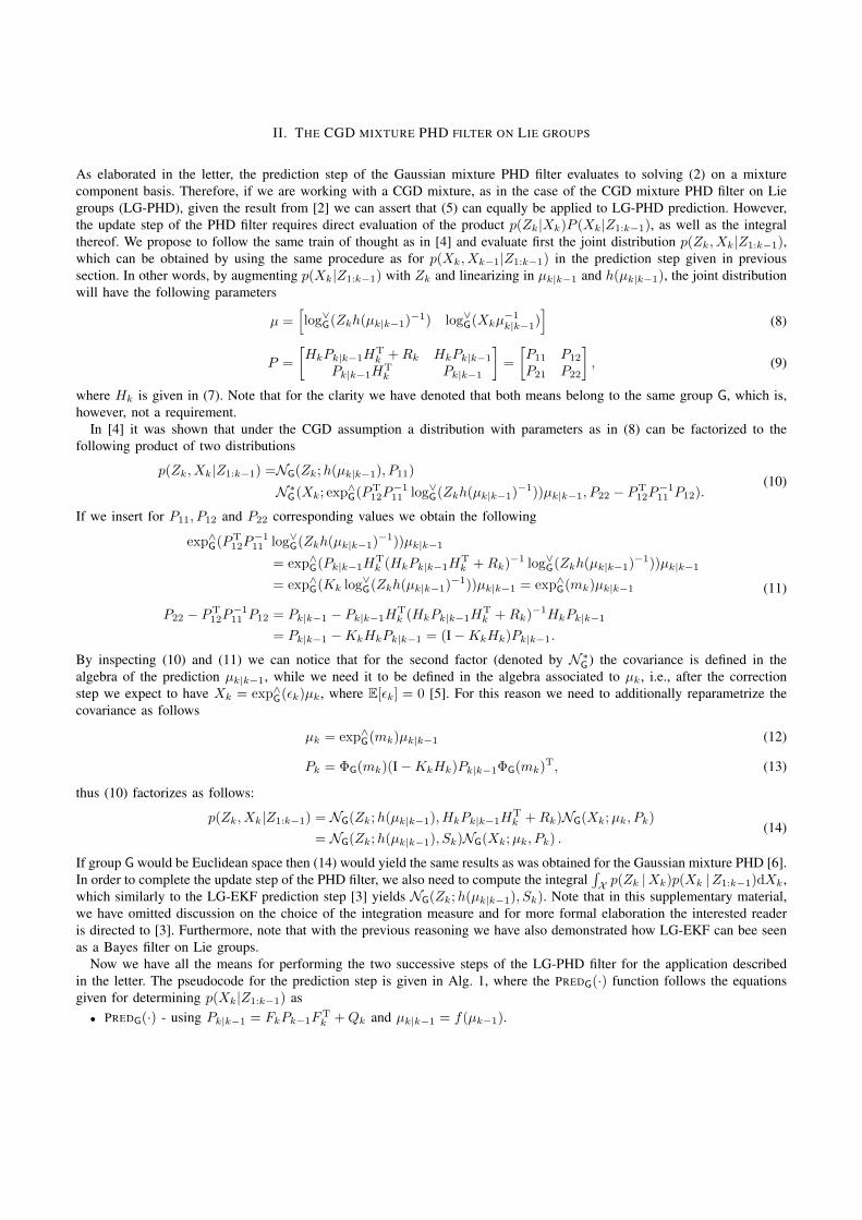
II. THE CGD MIXTURE PHD FILTER ON LIE GROUPS
As elaborated in the letter, the prediction step of the Gaussian mixture PHD filter evaluates to solving (2) on a mixturecomponent basis. Therefore, if we are working with a CGD mixture, as in the case of the CGD mixture PHD filter on Liegroups (LG-PHD), given the result from [2] we can assert that (5) can equally be applied to LG-PHD prediction. However,the update step of the PHD filter requires direct evaluation of the product p(Zk|Xk)P (Xk|Z1:k−1), as well as the integralthereof. We propose to follow the same train of thought as in [4] and evaluate first the joint distribution p(Zk, Xk|Z1:k−1),which can be obtained by using the same procedure as for p(Xk, Xk−1|Z1:k−1) in the prediction step given in previoussection. In other words, by augmenting p(Xk|Z1:k−1) with Zk and linearizing in µk|k−1 and h(µk|k−1), the joint distributionwill have the following parameters
µ =[log∨G(Zkh(µk|k−1)−1) log∨G(Xkµ
−1k|k−1)
](8)
P =
[HkPk|k−1HT
k +Rk HkPk|k−1Pk|k−1HT
k Pk|k−1
]=
[P11 P12
P21 P22
], (9)
where Hk is given in (7). Note that for the clarity we have denoted that both means belong to the same group G, which is,however, not a requirement.
In [4] it was shown that under the CGD assumption a distribution with parameters as in (8) can be factorized to thefollowing product of two distributions
p(Zk, Xk|Z1:k−1) =NG(Zk;h(µk|k−1), P11)
N ∗G(Xk; exp∧G(PT12P
−111 log∨G(Zkh(µk|k−1)−1))µk|k−1, P22 − PT
12P−111 P12).
(10)
If we insert for P11, P12 and P22 corresponding values we obtain the following
exp∧G(PT12P
−111 log∨G(Zkh(µk|k−1)−1))µk|k−1
= exp∧G(Pk|k−1HTk (HkPk|k−1H
Tk +Rk)−1 log∨G(Zkh(µk|k−1)−1))µk|k−1
= exp∧G(Kk log∨G(Zkh(µk|k−1)−1))µk|k−1 = exp∧G(mk)µk|k−1
P22 − PT12P
−111 P12 = Pk|k−1 − Pk|k−1H
Tk (HkPk|k−1H
Tk +Rk)−1HkPk|k−1
= Pk|k−1 −KkHkPk|k−1 = (I−KkHk)Pk|k−1.
(11)
By inspecting (10) and (11) we can notice that for the second factor (denoted by N ∗G ) the covariance is defined in thealgebra of the prediction µk|k−1, while we need it to be defined in the algebra associated to µk, i.e., after the correctionstep we expect to have Xk = exp∧G(εk)µk, where E[εk] = 0 [5]. For this reason we need to additionally reparametrize thecovariance as follows
µk = exp∧G(mk)µk|k−1 (12)
Pk = ΦG(mk)(I−KkHk)Pk|k−1ΦG(mk)T, (13)
thus (10) factorizes as follows:
p(Zk, Xk|Z1:k−1) = NG(Zk;h(µk|k−1), HkPk|k−1HTk +Rk)NG(Xk;µk, Pk)
= NG(Zk;h(µk|k−1), Sk)NG(Xk;µk, Pk) .(14)
If group G would be Euclidean space then (14) would yield the same results as was obtained for the Gaussian mixture PHD [6].In order to complete the update step of the PHD filter, we also need to compute the integral
∫X p(Zk |Xk)p(Xk |Z1:k−1)dXk,
which similarly to the LG-EKF prediction step [3] yields NG(Zk;h(µk|k−1), Sk). Note that in this supplementary material,we have omitted discussion on the choice of the integration measure and for more formal elaboration the interested readeris directed to [3]. Furthermore, note that with the previous reasoning we have also demonstrated how LG-EKF can bee seenas a Bayes filter on Lie groups.
Now we have all the means for performing the two successive steps of the LG-PHD filter for the application describedin the letter. The pseudocode for the prediction step is given in Alg. 1, where the PREDG(·) function follows the equationsgiven for determining p(Xk|Z1:k−1) as• PREDG(·) - using Pk|k−1 = FkPk−1FT
k +Qk and µk|k−1 = f(µk−1).

Algorithm 1 The prediction step of the LG-PHD filter
Require: wik−1,Gik−1
Jk−1
i=1 , wb,ik ,Gb,ik
Jbk
i=1, pS
1: j ← 0 (initialization)2: for i := 1 to Jb
k (# of newly born components) do3: wj
k|k−1 ← wb,ik ; Gjk|k−1 ← G
b,ik ; j ← j + 1
4: end for5: for i := 1 to Jk−1 (# of components existing at k − 1) do6: wj
k|k−1 ← pS wbk−1 ; Gjk|k−1 ← PREDG(Gik−1) ; j ← j + 1
7: end for8: Jk|k−1 ← j (# of predicted components)9: return wi
k|k−1,Gik|k−1Jk|k−1
i=1
In the particular application presented in the letter, where we assume that the objects were following the constant velocitySE(2)× R3 motion model assumption [7], the motion model f(µk−1) and the Jacobian F are given as
f(µk−1) = µk−1 exp∧G
[Tvk−1
0
], (15)
F = − d
ds
(log∨G
(f(µk−1)f(exp∧G(s)µk−1)−1
))∣∣∣∣s=0
= − d
ds
(log∨G
(µk−1 exp∧G
[Tvk−1
0
](exp∧G(s)µk−1 exp∧G
[T (svel + vk−1)
0
])−1))∣∣∣∣∣
s=0
= − d
ds
(log∨G
(µk−1 exp∧G
[Tvk−1
0
]exp∧G
[T (svel + vk−1)
0
]−1µ−1k−1 exp∧G(s)−1
))∣∣∣∣∣s=0
= − d
ds
(log∨G
(exp∧G
(AdG
(µk−1
) [Tvk−10
])µk−1
µ−1k−1 exp∧G
(AdG
(µk−1
) [T (svel + vk−1)0
])−1exp∧G(s)−1
))∣∣∣∣∣s=0
≈ − d
ds
(log∨G
(exp∧G
(ΦG
(AdG
(µk−1
) [Tvk−10
])AdG
(µk−1
) [−Tsvel
0
])exp∧G(s)−1
))∣∣∣∣∣s=0
≈ − d
ds
(ΦG
(AdG
(µk−1
) [Tvk−10
])AdG
(µk−1
) [−Tsvel
0
]− s)∣∣∣∣∣
s=0
=
I TΦSE(2)
(T AdSE(2)
(µposk−1)vk−1
)AdSE(2)
(µposk−1)
0 I
, (16)
where µk−1 consists of positional and velocity part constructed by placing the SE(2) and R3 components block-diagonally, such that µk−1 = blkdiag(µpos
k−1, µvelk−1), vk−1 = log∨R(µvel
k−1), and accordingly s = [spos svel]T and AdG(µ) =blkdiag(AdSE(2)(µ
pos),AdR3(µvel)). The parameter T represents the discretization time. To obtain the second-to-last step,the following Baker-Campbell-Hausdorff formula was used
log∨G(exp∧(−x) exp∧(x+ y)) = ΦG(−x)y +O(||y||2). (17)
The pseudocode for the update step is given in Alg. 2. The algorithm employs several outlying functions including:
• INNOVG′(·, ·) - using νi,jk =[logG′
(Zjkh(µi
k|k−1)−1)]∨
G′, Si,j
k = Hi,jk P i,j
k|k−1Hi,jT
k +Rk,
• CORRECTR(·, ·) - using wi,jk =
pDwik|k−1q
i,jk (Z)
λZc(Z) + pD∑Jk|k−1
l=1 wlk|k−1q
l,jk (Z)
, where qi,jk (Z) = N (Zjk;h(µi
k|k−1), Si,jk ),
• REPARAMG(·, ·) - using (12) and (13),• REDUCTIONG(·) - employing reduction schemes as described in the letter.
For the multitarget tracking application given in the letter, since the measurement arises as a SE(2) member, i.e., h(Xk) = Xk
and the measurement Jacobian Hk evaluates to Hk =[I 0
].
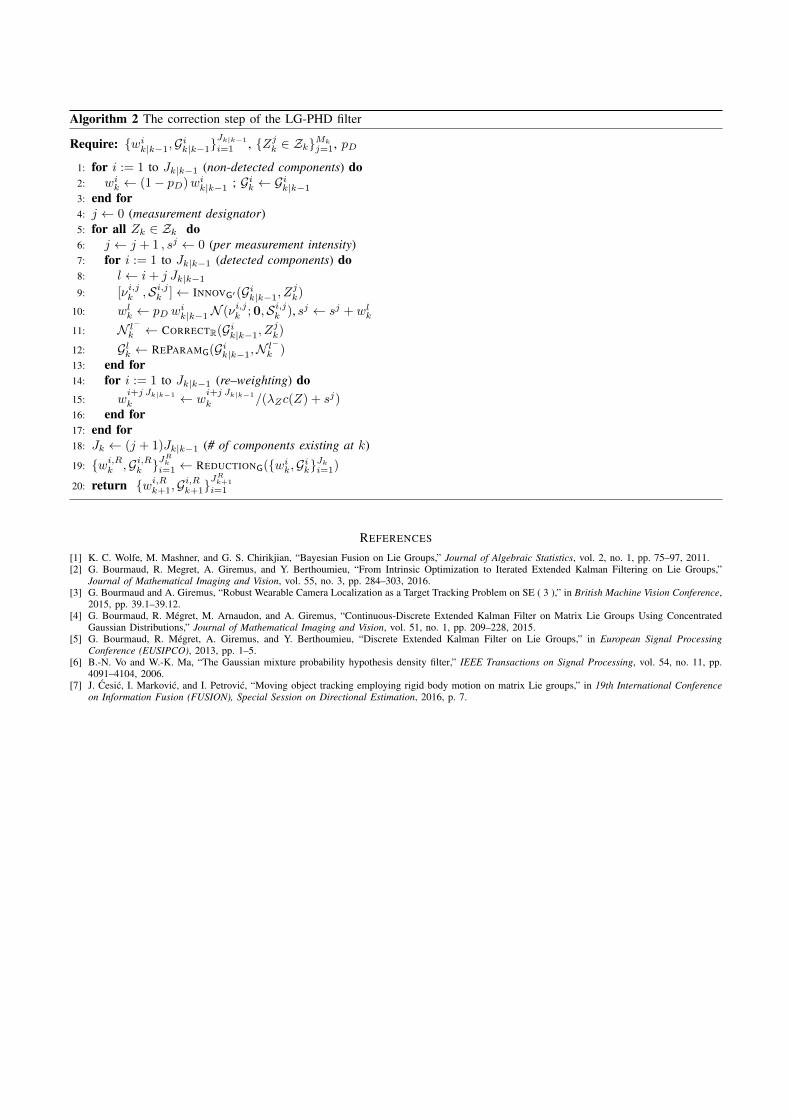
Algorithm 2 The correction step of the LG-PHD filter
Require: wik|k−1,Gik|k−1
Jk|k−1
i=1 , Zjk ∈ ZkMk
j=1, pD
1: for i := 1 to Jk|k−1 (non-detected components) do2: wi
k ← (1− pD)wik|k−1 ; Gik ← Gik|k−1
3: end for4: j ← 0 (measurement designator)5: for all Zk ∈ Zk do6: j ← j + 1 , sj ← 0 (per measurement intensity)7: for i := 1 to Jk|k−1 (detected components) do8: l← i+ j Jk|k−19: [νi,jk ,Si,jk ]← INNOVG′(Gik|k−1, Z
jk)
10: wlk ← pD w
ik|k−1N (νi,jk ;0,Si,jk ), sj ← sj + wl
k
11: N l−k ← CORRECTR(Gik|k−1, Z
jk)
12: Glk ← REPARAMG(Gik|k−1,N l−k )
13: end for14: for i := 1 to Jk|k−1 (re–weighting) do15: w
i+j Jk|k−1
k ← wi+j Jk|k−1
k /(λZc(Z) + sj)16: end for17: end for18: Jk ← (j + 1)Jk|k−1 (# of components existing at k)
19: wi,Rk ,Gi,Rk
JRk
i=1 ← REDUCTIONG(wik,GikJk
i=1)
20: return wi,Rk+1,G
i,Rk+1
JRk+1
i=1
REFERENCES
[1] K. C. Wolfe, M. Mashner, and G. S. Chirikjian, “Bayesian Fusion on Lie Groups,” Journal of Algebraic Statistics, vol. 2, no. 1, pp. 75–97, 2011.[2] G. Bourmaud, R. Megret, A. Giremus, and Y. Berthoumieu, “From Intrinsic Optimization to Iterated Extended Kalman Filtering on Lie Groups,”
Journal of Mathematical Imaging and Vision, vol. 55, no. 3, pp. 284–303, 2016.[3] G. Bourmaud and A. Giremus, “Robust Wearable Camera Localization as a Target Tracking Problem on SE ( 3 ),” in British Machine Vision Conference,
2015, pp. 39.1–39.12.[4] G. Bourmaud, R. Megret, M. Arnaudon, and A. Giremus, “Continuous-Discrete Extended Kalman Filter on Matrix Lie Groups Using Concentrated
Gaussian Distributions,” Journal of Mathematical Imaging and Vision, vol. 51, no. 1, pp. 209–228, 2015.[5] G. Bourmaud, R. Megret, A. Giremus, and Y. Berthoumieu, “Discrete Extended Kalman Filter on Lie Groups,” in European Signal Processing
Conference (EUSIPCO), 2013, pp. 1–5.[6] B.-N. Vo and W.-K. Ma, “The Gaussian mixture probability hypothesis density filter,” IEEE Transactions on Signal Processing, vol. 54, no. 11, pp.
4091–4104, 2006.[7] J. Cesic, I. Markovic, and I. Petrovic, “Moving object tracking employing rigid body motion on matrix Lie groups,” in 19th International Conference
on Information Fusion (FUSION), Special Session on Directional Estimation, 2016, p. 7.

curriculum vitae
Josip Ćesić was born in Zagreb, Croatia in 1989. He nished XV Gymnasium (MIOC)
in Zagreb in 2008 and received his BSc and MSc degree (Magna Cum Laude) in electrical
engineering and information technology from the University of Zagreb, Faculty of Electrical
Engineering and Computing (UNIZG-FER) in 2011 and 2013, respectively. He nished the
third semester of his master program at Chalmers University of Technology, Sweden, as an
exchange student.
During the undergraduate studies he received Dean’s Award Josip Lončar and Special
Dean’s Award Josip Lončar for outstanding achievements on the rst year of studies and
the overall BSc level, respectively. During the graduate studies he received Rector’s Award
and Special Rector’s Award for practical applications in the elds of robotics and control
systems. He was also awarded with scholarships from the Croatian Ministry of Science
(2008-2009), Scholarship of the University of Zagreb (2009-2010) and Scholarship of the
City of Zagreb (2010-2013).
He is employed as a research assistant at the Department of Control and Computer En-
gineering at FER Zagreb since April 2013. Since then, he was actively participating in several
international scientic projects, i.e., Computer Vision Innovations for Safe Trac (VISTA),
Advanced Technologies in Power Plants and Rail Vehicles (FER-KIET) and Cooperative
cloud based simultaneous localization and mapping in dynamic environments (cloudSLAM).
His main research interests are in the areas of autonomous systems and mobile robotics,
estimation theory and sensor processing, particularly employing radar, lidar and stereo
systems. He is an author or co-author of a book chapter, 7 papers published in peer-reviewed
journals and 13 papers presented at international conferences.e full list of publications is
given below.
137

Full list of publications
book chapters :
1. J. Ćesić, I. Marković, S. Jurić-Kavelj and I. Petrović. Short-TermMap Based Detection
and Tracking of Moving Objects with 3D Laser on a Vehicle. Informatics in Control,
Automation and Robotics, Lecture Notes in Electrical Engineering, Vol. 370, Joaquim
Filipe, Oleg Gusikhin, Kurosh Madani, Jurek Sasiadek (ed.), Cham, Switzerland :
Springer International Publishing, 205–222, 2016.
journal publications :
1. J. Ćesić, I. Marković and I. Petrović. Mixture Reduction on Matrix Lie Groups. IEEE
Signal Processing Letters, 24(11):1719–1723, 2017, IF: 2.528 (Q2).
2. I. Cvišić, J. Ćesić, I. Marković and I. Petrović. SOFT-SLAM: Computationally Ecient
Stereo Visual SLAM for Autonomous UAVs. Journal of Field Robotics, (accepted for
publication), DOI: 10.1002/rob.21762, 2017, IF: 4.882 (Q1).
3. J. Ćesić, I. Marković, M. Bukal and I. Petrović. Extended Information Filter onMatrix
Lie Groups. Automatica, 53(9):226–234, 2017, IF: 5.451 (Q1).
4. I.Marković, M. Bukal, J.Ćesić and I. Petrović. Multitarget tracking with the vonMises-
Fisher lter and probabilistic data association. Journal of Advances in Information
Fusion, (accepted for publication) 2017.
5. J. Ćesić, I. Marković, I. Cvišić and I. Petrović. Radar and stereo vision fusion for
multitarget tracking on the special Euclidean group. Robotics and autonomous systems,
83:338–348, 2016, IF: 1.950 (Q2).
6. I. Marković, J. Ćesić and I. Petrović. Von Mises Mixture PHD Filter. IEEE Signal
Processing Letters, 22(12):2229–2233, 2015, IF: 1.661 (Q2).
7. M. Orsag, J. Ćesić, T. Haus and S. Bogdan. Spincopter Wing Design and Flight
Control. Journal of intelligent & robotic systems, 70(1/4):165–179, 2013, IF: 0.932 (Q3).
conference publications :
1. K. Lenac, J. Ćesić, I. Marković and I. Petrović. Cooperative Cloud SLAM on Matrix
Lie Groups. ird Iberian Robotics Conference (Robot2017) Sevilla, Spain, (accepted
for publication) 2017.
2. K. Lenac, J. Ćesić, I. Marković, I. Cvišić and I. Petrović. Revival of ltering based
SLAM? Exactly sparse delayed state lter on Lie groups. IEEE/RSJ International Con-
ference on Intelligent Robots and Systems (IROS) Vancouver, Canada, pages 1012–1018,
2017.

3. V. Joukov, J. Ćesić, K. Westermann, I. Marković, D. Kulić and I. Petrović. Human
motion estimation on Lie groups using IMUmeasurements. IEEE/RSJ International
Conference on Intelligent Robots and Systems (IROS) Vancouver, Canada, pages 1965–
1972, 2017.
4. J. Ćesić, V. Joukov, I. Petrović and D. Kulić. Full Body Human Motion Estimation
on Lie Groups Using 3D Marker Position Measurements. IEEE-RAS International
Conference on Humanoid Robotics (Humanoids2016). Cancun, Mexico, pages 826–
833, 2016.
5. J.Ćesić, I. Marković and I. Petrović. Moving object tracking employing rigid bodymo-
tion on matrix Lie groups. International Conference on Information Fusion (FUSION),
Special Session on Directional Estimation. Heidelberg, Germany, pages 2109–2115,
2016.
6. I. Marković, J. Ćesić and I. Petrović. On wrapping the Kalman lter and estimating
with the SO(2) group. International Conference on Information Fusion (FUSION),
Special Session on Directional Estimation. Heidelberg, Germany, pages 2245–2250,
2016.
7. M. Obrvan, J. Ćesić and I. Petrović. Appearance based vehicle detection by radar-
stereo vision integration. Second Iberian Robotics Conference ((Robot2015)). Lisbon,
Portugal, pages 437–449, 2015.
8. B. Novoselnik, J.Ćesić, M. Baotić and I. Petrović. NonlinearModel Predictive Control
for Energy Ecient Housing with Modern Construction Materials. IEEE Sensors
Applications Symposium (SAS). Zadar, Croatia, pages 266–271, 2015.
9. I. Marković, M. Bukal, J. Ćesić and I. Petrović. Direction-only tracking of moving
objects on the unit sphere via probabilistic data association. International Conference
on Information Fusion (FUSION), Special Session onDirectional Estimation. Salamanca,
Spain, 2014.
10. J.Ćesić, I.Marković, S. Jurić-Kavelj and I. Petrović. Detection and tracking of dynamic
objects using 3D laser range sensor on a mobile platform. International Conference
on Informatics in Control, Automation and Robotics (ICINCO). Wien, Austria, 2014.
11. J. Ćesić, I. Marković and I. Petrović. Tracking of multiple moving objects on the unit
sphere using a multiple-camera system on a mobile robot. International Conference
on Intelligent Autonomous Systems (IAS). Padua, Italy, pages 899–911, 2014.
12. N. Skeledžija, J. Ćesić, E. Kočo, V. Bachler, H. N. Vučemilo and H. Džapo. Smart
Home Automation System for Energy Ecient Housing. International Conven-
tion on Information and Communication Technology, Electronics andMicroelectronics
(MIPRO2014). Opatija, Croatia, pages 166–171, 2014.
13. J. Ćesić, M. Orsag and S. Bogdan. Spincopter wing design and ight control. Inter-
national Conference on Unmanned Aircra Systems (ICUAS12). Philadelphia, PA, USA,
2012.
životopis
Josip Ćesić rođen je u Zagrebu, Hrvatska, 1989. godine. Završio je XV. gimnaziju (MIOC)
u Zagrebu 2008. godine, dok je zvanje prvostupnika, odnosno magistra elektrotehnike
i informacijske tehnologije Sveučilišta u Zagrebu, Fakulteta elektrotehnike i računarstva
(UNIZG-FER) uz visoke počasti (Magna Cum Laude) stekao 2011., odnosno 2013. godine.
Treći semestar diplomskoga studija završio je na Tehničkom Svečilištu Chalmers, Švedska,
u sklopu studentske razmjene.
U sklopu preddiplomskoga studija dobitnik je Dekanove nagrade Josip Lončar i Posebne
dekanove nagrade Josip Lončar za istaknuti uspjeh na prvoj godini studija, odnosno tijekom
cjelokupnog preddiplomskog studija. Tijekom diplomskoga studija dobio je Rektorovu
nagradu te Posebnu Rektorovu nagradu za praktične primjene u području robotike i sustava
upravljanja. Također je nagrađen StipendijomMinistarstva znanosti i obrazovanja (2008.-
2009.), Stipendijom Sveučilišta u Zagrebu (2009.-2010.) i Stipendijom Grada Zagreba
(2010.-2013.).
Zaposlen je na mjestu asistenta na Zavodu za automatiku i računalno inženjerstvo na
UNIZG-FER od travnja 2013. godine. Od tada je aktivno sudjelovao u nekolikomeđunarodnih
istraživačkih projekata, i.e., Inovativni sustavi računalnog vida za siguran promet (VISTA),
Napredne tehnologije u elektroenergetskim postrojenjima i tračničkim vozilima (FER-KIET)
te Kooperativno simultano lokaliziranje i kartiranje dinamičkog prostora zasnovano na
uslugama u oblaku (cloudSLAM). Njegovi istraživački interesi uključuju autonomne sustave i
mobilnu robotiku, teoriju estimacije, obradu senzora s naglaskom na radare, lidare i stere-
ovizijske sustave. Autor je ili suautor poglavlja u knjizi, 7 znanstvenih radova u časopisima i
13 radova prezentiranih na međunarodnim konferencijama.
140

colophon
is document was typeset and inspired by the typographical look-and-feel classicthesis devel-
oped by André Miede, which was based on Robert Bringhurst’s book on typographye Elements of
Typographic Style, and by the FERElemental developed by Ivan Marković whose design was based
on FERBook developed by Jadranko Matuško.

