Multiple Logistic Regression - GitHub Pages Logistic... · 2.Perform multiple logistic regression...
45
4 Oct 2016 Intermediate Statistics 1 Multiple Logistic Regression Dr. Wan Nor Arifin Unit of Biostatistics and Research Methodology, Universiti Sains Malaysia. [email protected] / wnarifin.pancakeapps.com Wan Nor Arifin, 2015. Multiple logistic regression by Wan Nor Arifin is licensed under the Creative Commons Attribution- ShareAlike 4.0 International License. To view a copy of this license, visit http://creativecommons.org/licenses/by-sa/4.0/. IBM SPSS Statistics Version 22 screenshots are copyrighted to IBM Corp.
Transcript of Multiple Logistic Regression - GitHub Pages Logistic... · 2.Perform multiple logistic regression...

4 Oct 2016 Intermediate Statistics1
Multiple Logistic RegressionDr. Wan Nor Arifin
Unit of Biostatistics and Research Methodology,Universiti Sains Malaysia.
[email protected] / wnarifin.pancakeapps.com
Wan Nor Arifin, 2015. Multiple logistic regression by Wan Nor Arifin is licensed under the Creative Commons Attribution-ShareAlike 4.0 International License. To view a copy of this license, visit http://creativecommons.org/licenses/by-sa/4.0/.
IBM SPSS Statistics Version 22 screenshots are copyrighted to IBM Corp.
4 Oct 2016 Intermediate Statistics2
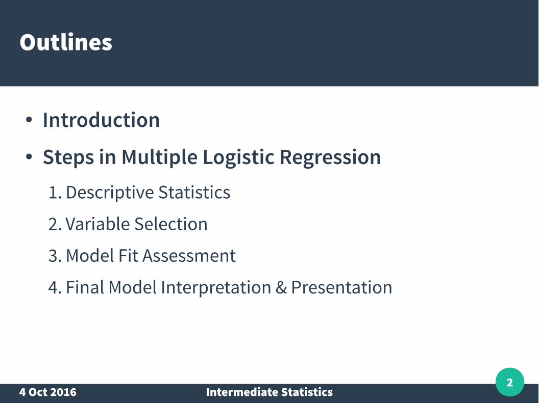
Outlines
● Introduction● Steps in Multiple Logistic Regression
1. Descriptive Statistics
2. Variable Selection
3. Model Fit Assessment
4. Final Model Interpretation & Presentation
4 Oct 2016 Intermediate Statistics3
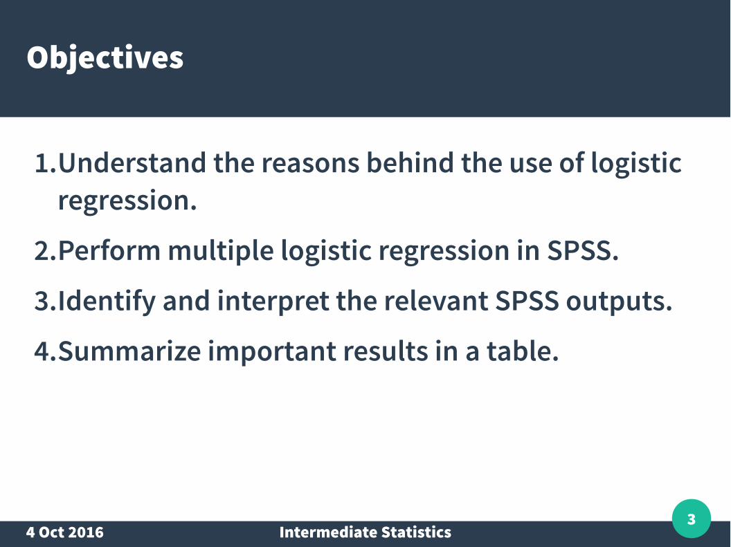
Objectives
1.Understand the reasons behind the use of logistic regression.
2.Perform multiple logistic regression in SPSS.
3.Identify and interpret the relevant SPSS outputs.
4.Summarize important results in a table.
4 Oct 2016 Intermediate Statistics4
Introduction
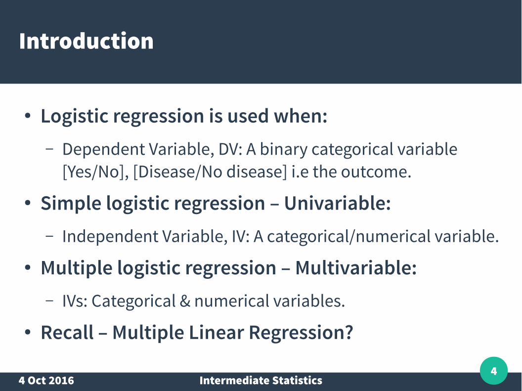
● Logistic regression is used when:– Dependent Variable, DV: A binary categorical variable
[Yes/No], [Disease/No disease] i.e the outcome.● Simple logistic regression – Univariable:
– Independent Variable, IV: A categorical/numerical variable.● Multiple logistic regression – Multivariable:
– IVs: Categorical & numerical variables.● Recall – Multiple Linear Regression?
4 Oct 2016 Intermediate Statistics5
Introduction
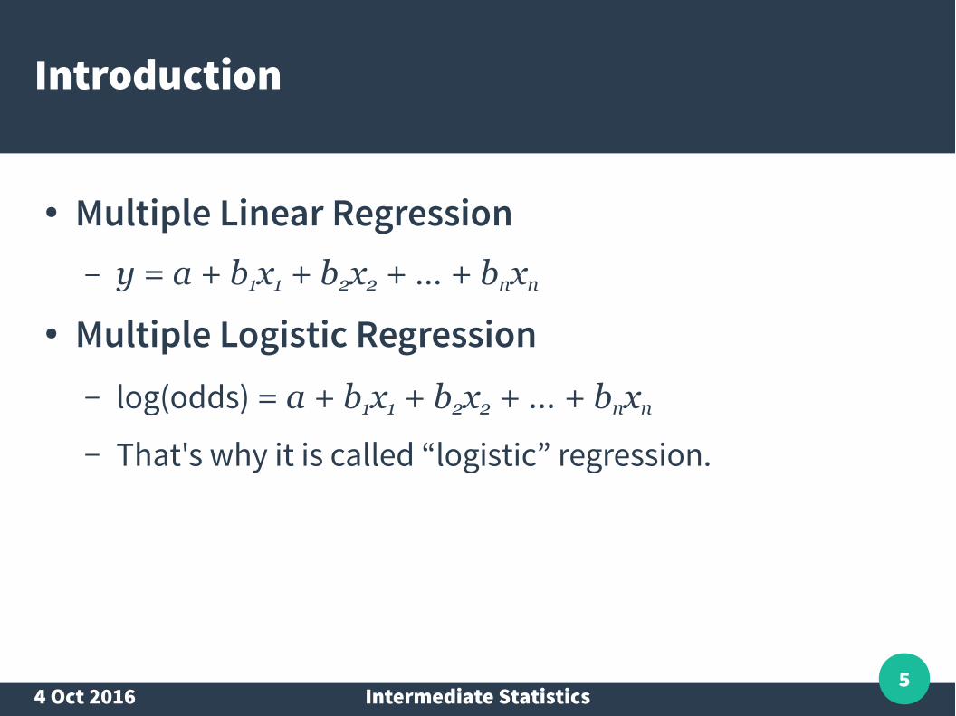
● Multiple Linear Regression– y = a + b1x1 + b2x2 + … + bnxn
● Multiple Logistic Regression– log(odds) = a + b1x1 + b2x2 + … + bnxn
– That's why it is called “logistic” regression.
4 Oct 2016 Intermediate Statistics6
Introduction
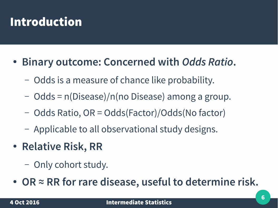
● Binary outcome: Concerned with Odds Ratio.– Odds is a measure of chance like probability.– Odds = n(Disease)/n(no Disease) among a group.– Odds Ratio, OR = Odds(Factor)/Odds(No factor)– Applicable to all observational study designs.
● Relative Risk, RR– Only cohort study.
● OR ≈ RR for rare disease, useful to determine risk.
4 Oct 2016 Intermediate Statistics7
Introduction
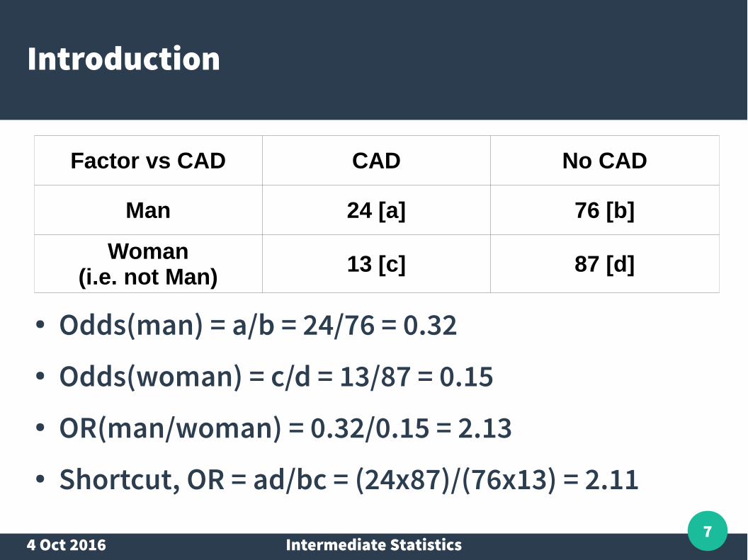
● Odds(man) = a/b = 24/76 = 0.32● Odds(woman) = c/d = 13/87 = 0.15● OR(man/woman) = 0.32/0.15 = 2.13● Shortcut, OR = ad/bc = (24x87)/(76x13) = 2.11
Factor vs CAD CAD No CAD
Man 24 [a] 76 [b]
Woman(i.e. not Man)
13 [c] 87 [d]
4 Oct 2016 Intermediate Statistics8
Introduction
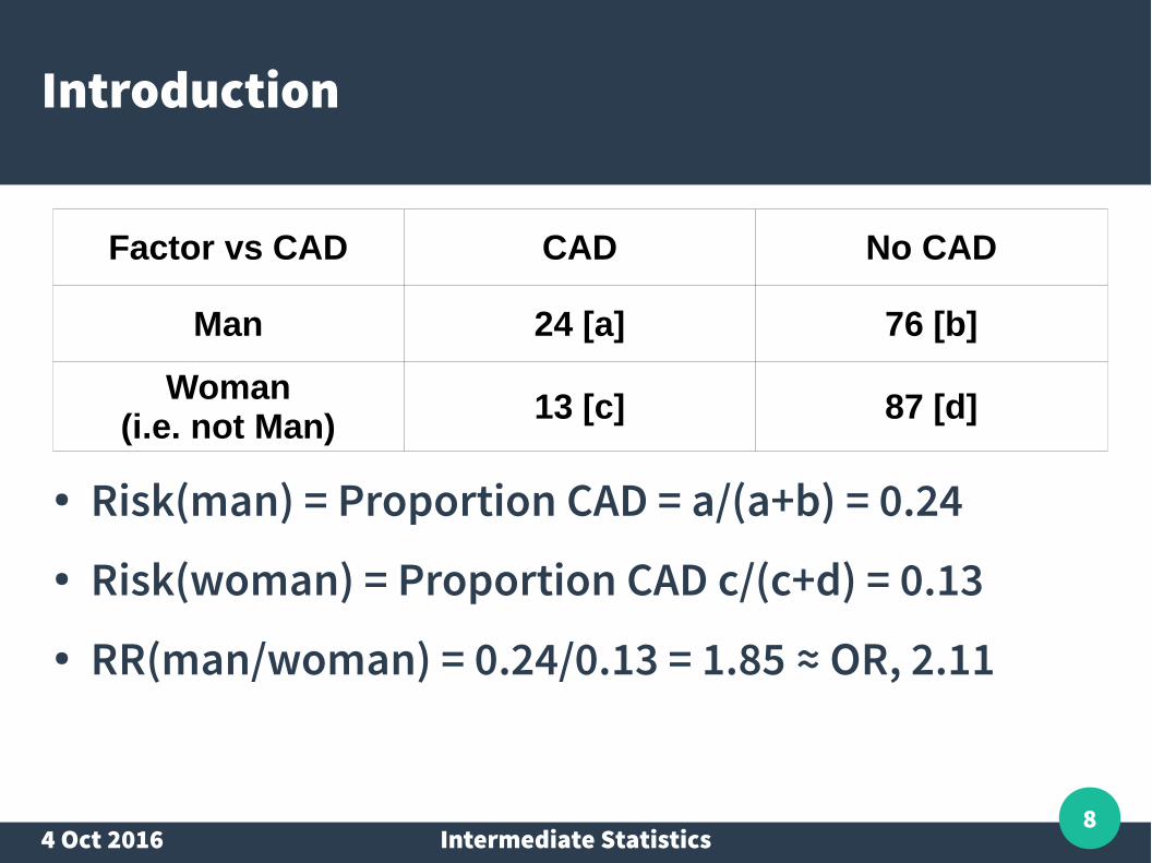
● Risk(man) = Proportion CAD = a/(a+b) = 0.24● Risk(woman) = Proportion CAD c/(c+d) = 0.13● RR(man/woman) = 0.24/0.13 = 1.85 ≈ OR, 2.11
Factor vs CAD CAD No CAD
Man 24 [a] 76 [b]
Woman(i.e. not Man)
13 [c] 87 [d]
4 Oct 2016 Intermediate Statistics9
Steps in Multiple Logistic Regression
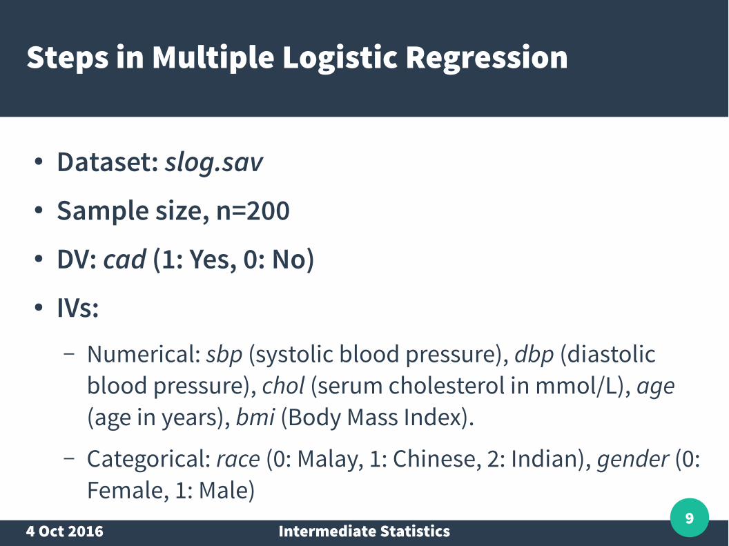
● Dataset: slog.sav● Sample size, n=200● DV: cad (1: Yes, 0: No)● IVs:
– Numerical: sbp (systolic blood pressure), dbp (diastolic blood pressure), chol (serum cholesterol in mmol/L), age (age in years), bmi (Body Mass Index).
– Categorical: race (0: Malay, 1: Chinese, 2: Indian), gender (0: Female, 1: Male)
4 Oct 2016 Intermediate Statistics10
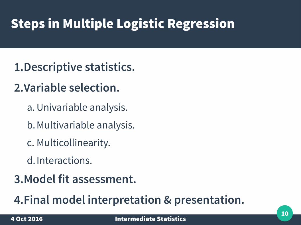
Steps in Multiple Logistic Regression
1.Descriptive statistics.
2.Variable selection.a. Univariable analysis.
b. Multivariable analysis.
c. Multicollinearity.
d. Interactions.
3.Model fit assessment.
4.Final model interpretation & presentation.
4 Oct 2016 Intermediate Statistics11
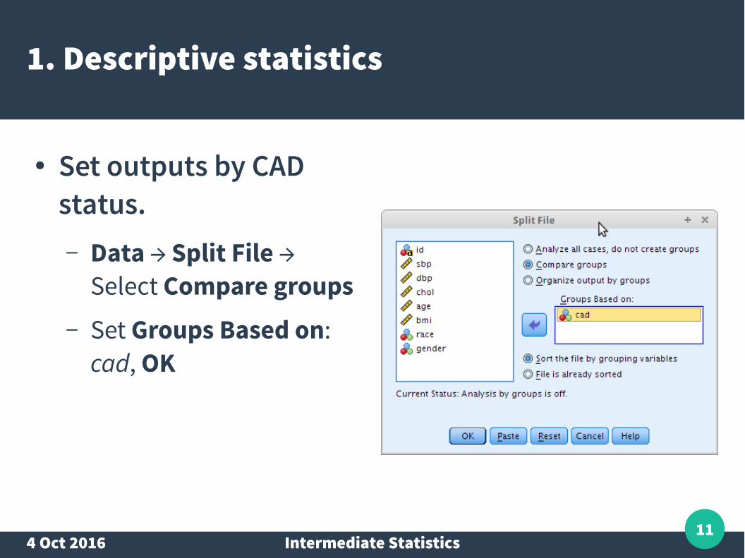
1. Descriptive statistics
● Set outputs by CAD status.– Data → Split File →
Select Compare groups– Set Groups Based on:
cad, OK
4 Oct 2016 Intermediate Statistics12
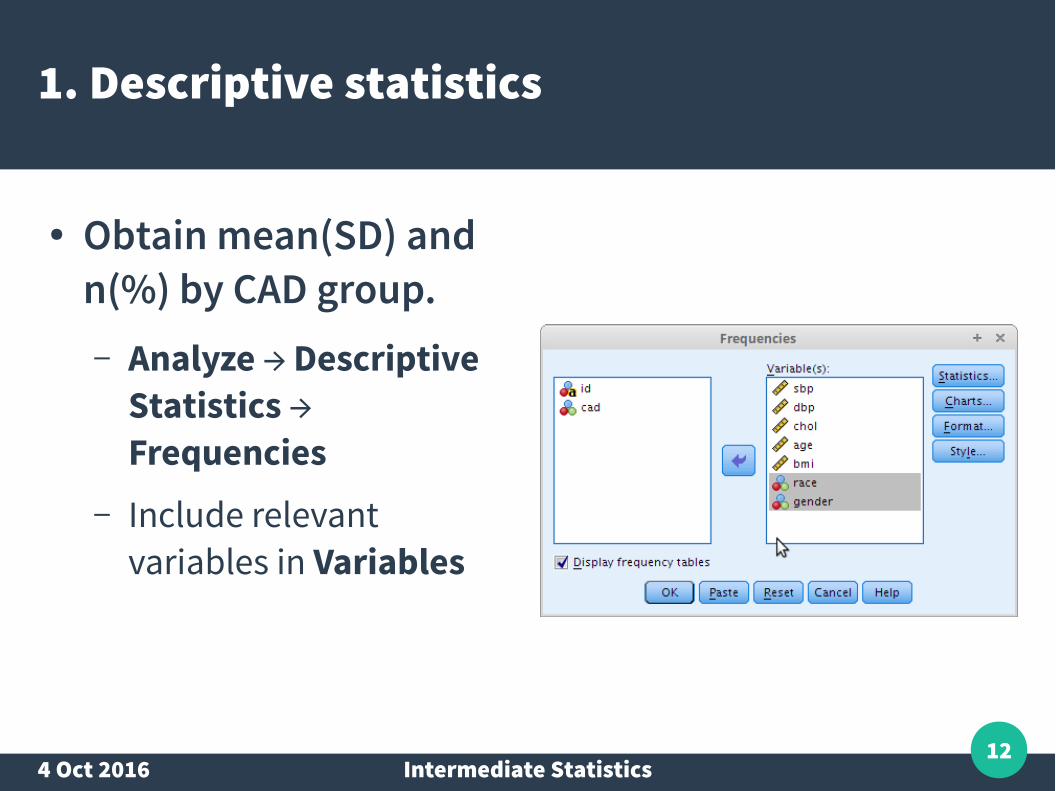
1. Descriptive statistics
● Obtain mean(SD) and n(%) by CAD group.– Analyze → Descriptive
Statistics → Frequencies
– Include relevant variables in Variables
4 Oct 2016 Intermediate Statistics13
1. Descriptive statistics
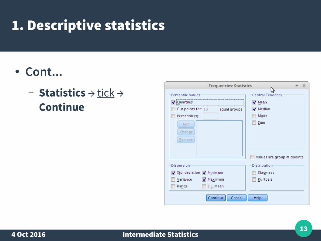
● Cont...– Statistics → tick →
Continue
4 Oct 2016 Intermediate Statistics14
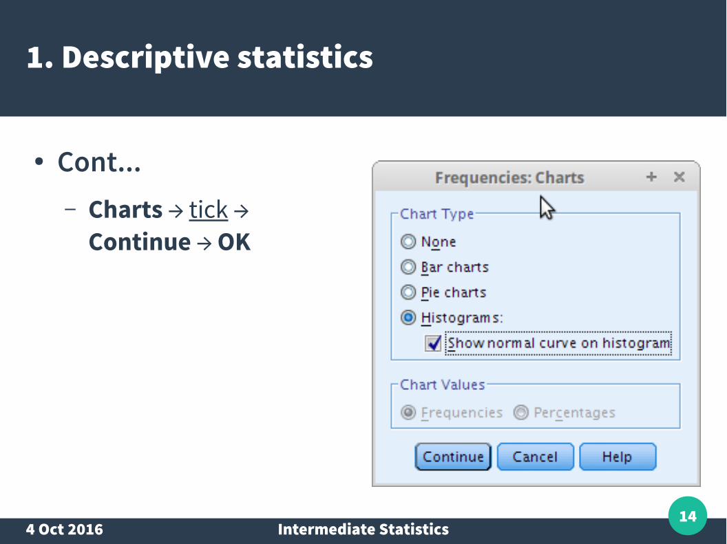
1. Descriptive statistics
● Cont...– Charts → tick →
Continue → OK
4 Oct 2016 Intermediate Statistics15
1. Descriptive statistics
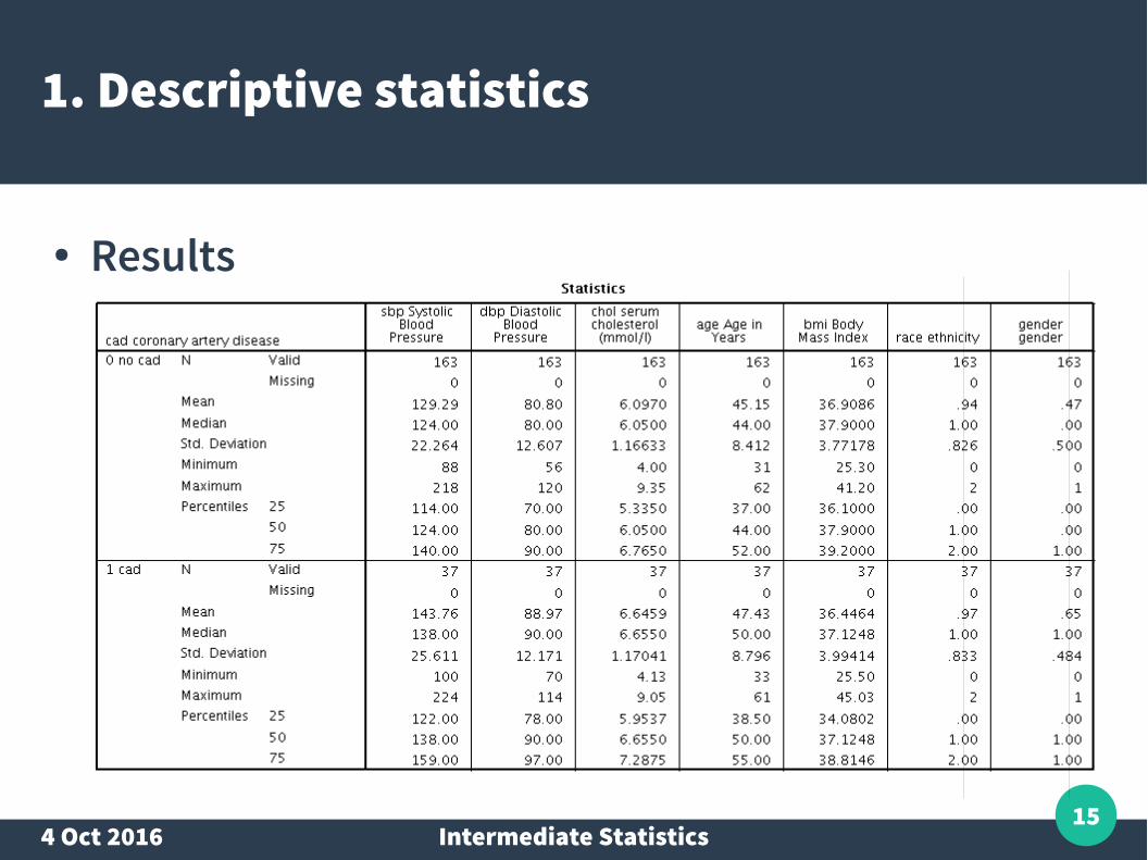
● Results
4 Oct 2016 Intermediate Statistics16
1. Descriptive statistics
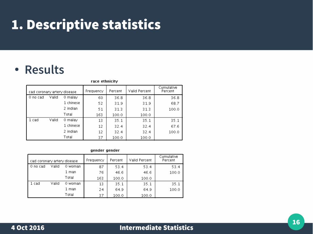
● Results
4 Oct 2016 Intermediate Statistics17
1. Descriptive statistics
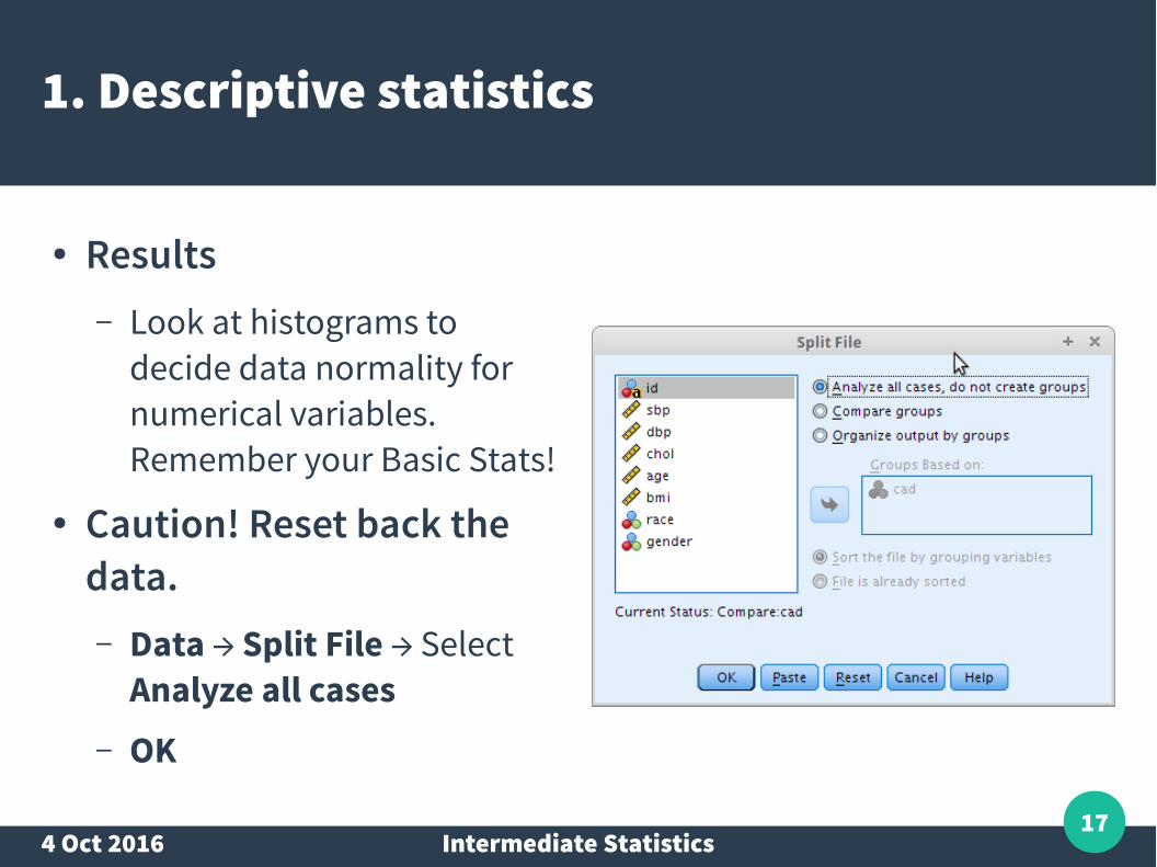
● Results– Look at histograms to
decide data normality for numerical variables. Remember your Basic Stats!
● Caution! Reset back the data.– Data → Split File → Select
Analyze all cases– OK
4 Oct 2016 Intermediate Statistics18
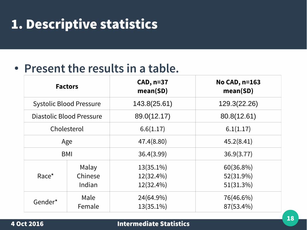
1. Descriptive statistics
● Present the results in a table.Factors CAD, n=37
mean(SD)No CAD, n=163
mean(SD)
Systolic Blood Pressure 143.8(25.61) 129.3(22.26)
Diastolic Blood Pressure 89.0(12.17) 80.8(12.61)
Cholesterol 6.6(1.17) 6.1(1.17)
Age 47.4(8.80) 45.2(8.41)
BMI 36.4(3.99) 36.9(3.77)
Race*Malay
ChineseIndian
13(35.1%)12(32.4%)12(32.4%)
60(36.8%)52(31.9%)51(31.3%)
Gender* MaleFemale
24(64.9%)13(35.1%)
76(46.6%)87(53.4%)
4 Oct 2016 Intermediate Statistics19
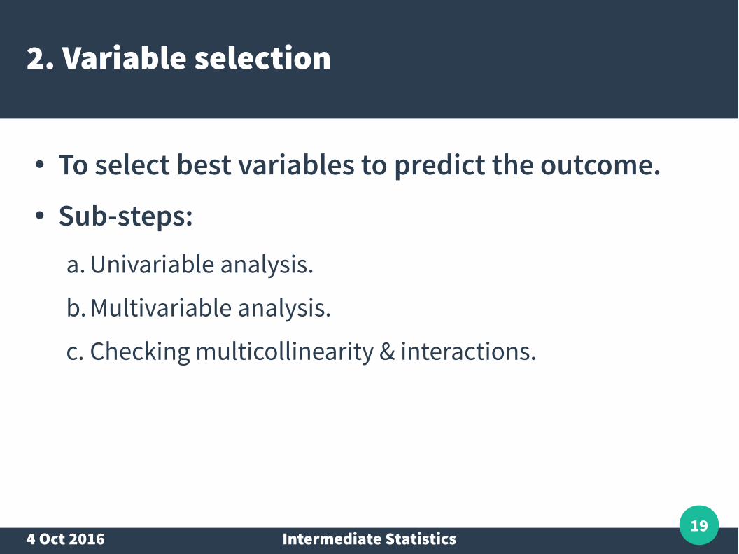
2. Variable selection
● To select best variables to predict the outcome.● Sub-steps:
a. Univariable analysis.
b. Multivariable analysis.
c. Checking multicollinearity & interactions.
4 Oct 2016 Intermediate Statistics20
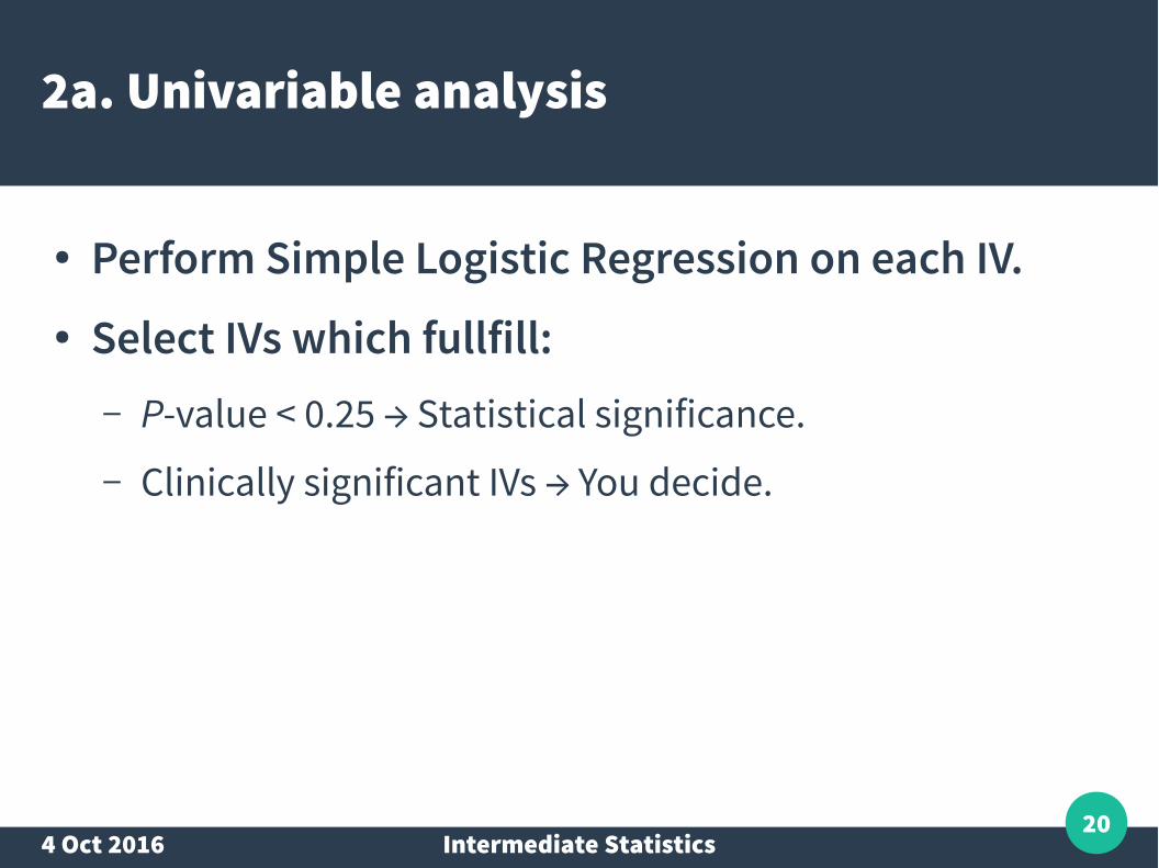
2a. Univariable analysis
● Perform Simple Logistic Regression on each IV.● Select IVs which fullfill:
– P-value < 0.25 → Statistical significance.– Clinically significant IVs → You decide.
4 Oct 2016 Intermediate Statistics21
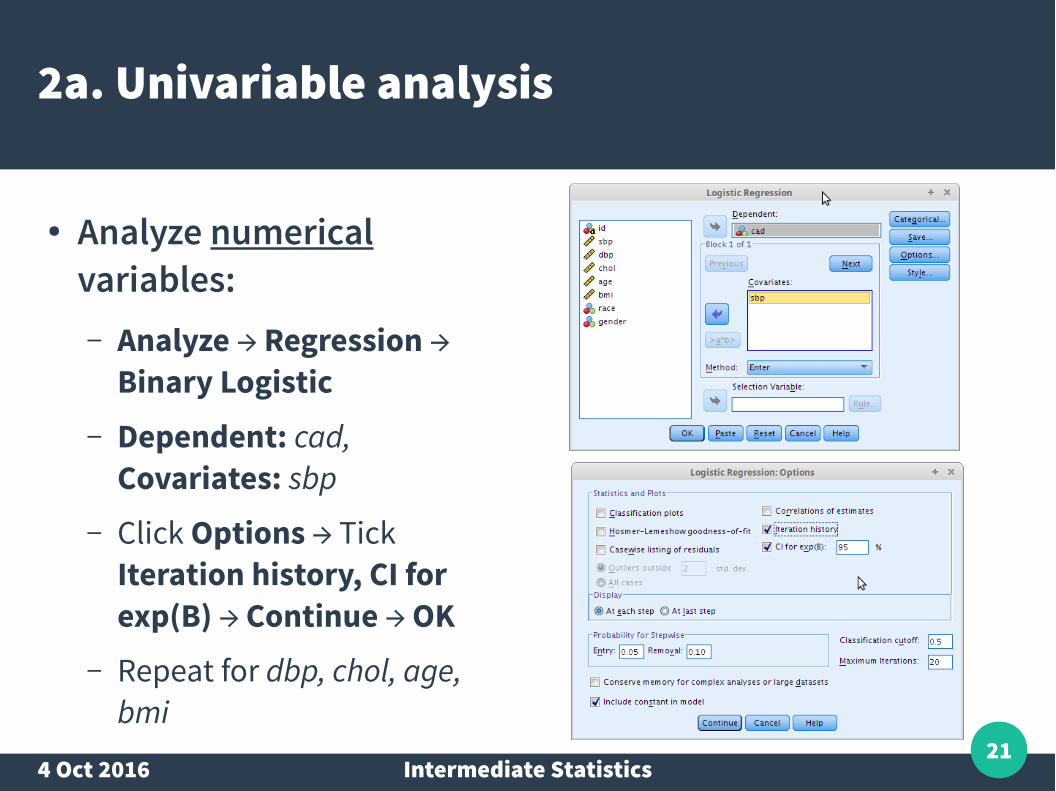
2a. Univariable analysis
● Analyze numerical variables:– Analyze → Regression →
Binary Logistic– Dependent: cad,
Covariates: sbp– Click Options → Tick
Iteration history, CI for exp(B) → Continue → OK
– Repeat for dbp, chol, age, bmi
4 Oct 2016 Intermediate Statistics22
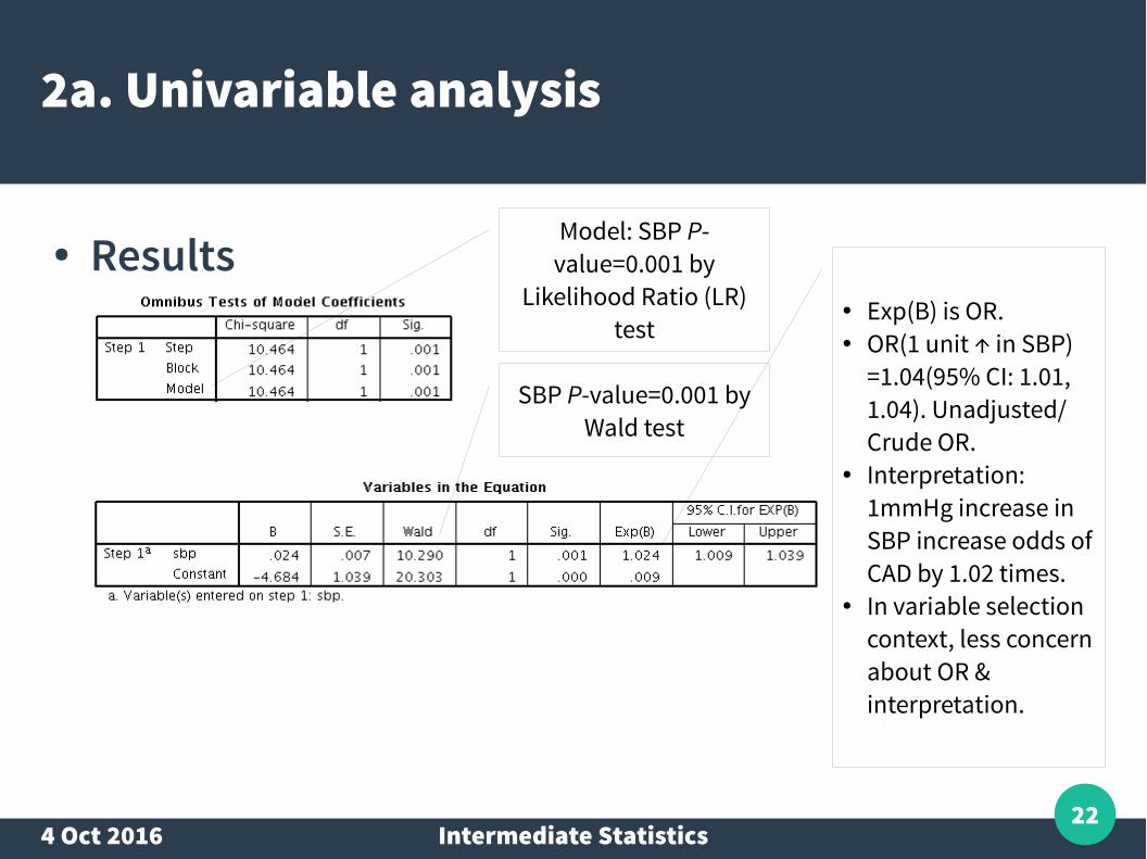
2a. Univariable analysis
● ResultsModel: SBP P-
value=0.001 by Likelihood Ratio (LR)
test
SBP P-value=0.001 by Wald test
● Exp(B) is OR.● OR(1 unit ↑ in SBP)
=1.04(95% CI: 1.01, 1.04). Unadjusted/ Crude OR.
● Interpretation: 1mmHg increase in SBP increase odds of CAD by 1.02 times.
● In variable selection context, less concern about OR & interpretation.
4 Oct 2016 Intermediate Statistics23
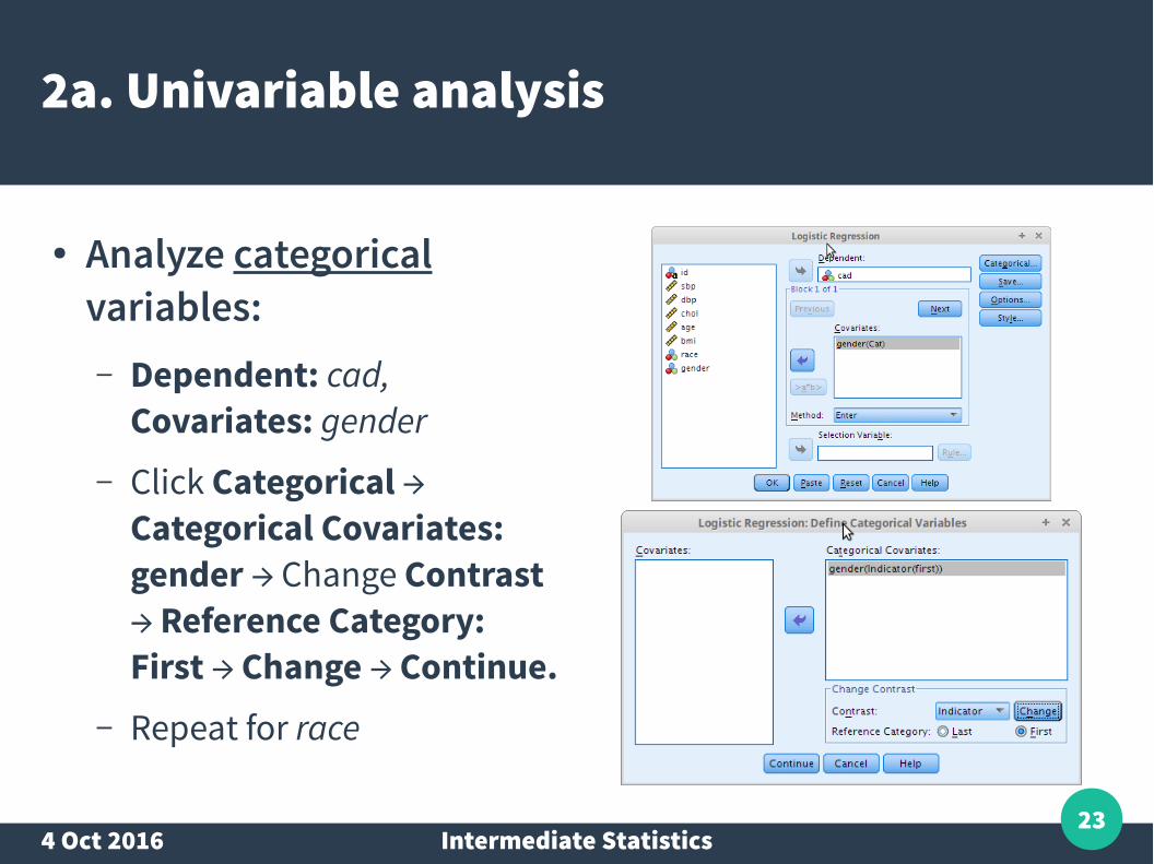
2a. Univariable analysis
● Analyze categorical variables:– Dependent: cad,
Covariates: gender
– Click Categorical → Categorical Covariates: gender → Change Contrast → Reference Category: First → Change → Continue.
– Repeat for race
4 Oct 2016 Intermediate Statistics24
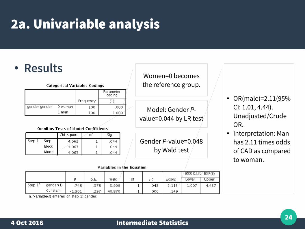
2a. Univariable analysis
● ResultsWomen=0 becomes the reference group.
Model: Gender P-value=0.044 by LR test
Gender P-value=0.048 by Wald test
● OR(male)=2.11(95% CI: 1.01, 4.44). Unadjusted/Crude OR.
● Interpretation: Man has 2.11 times odds of CAD as compared to woman.
4 Oct 2016 Intermediate Statistics25
2a. Univariable analysis
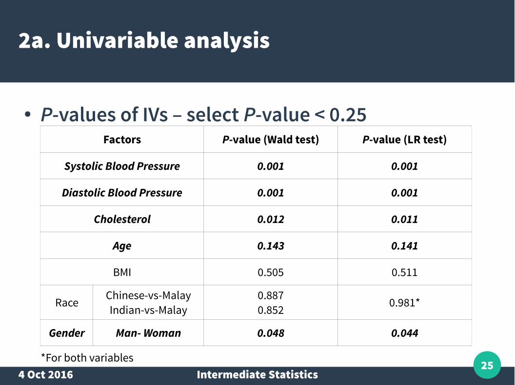
● P-values of IVs – select P-value < 0.25Factors P-value (Wald test) P-value (LR test)
Systolic Blood Pressure 0.001 0.001
Diastolic Blood Pressure 0.001 0.001
Cholesterol 0.012 0.011
Age 0.143 0.141
BMI 0.505 0.511
Race Chinese-vs-MalayIndian-vs-Malay
0.8870.852 0.981*
Gender Man- Woman 0.048 0.044
*For both variables
4 Oct 2016 Intermediate Statistics26
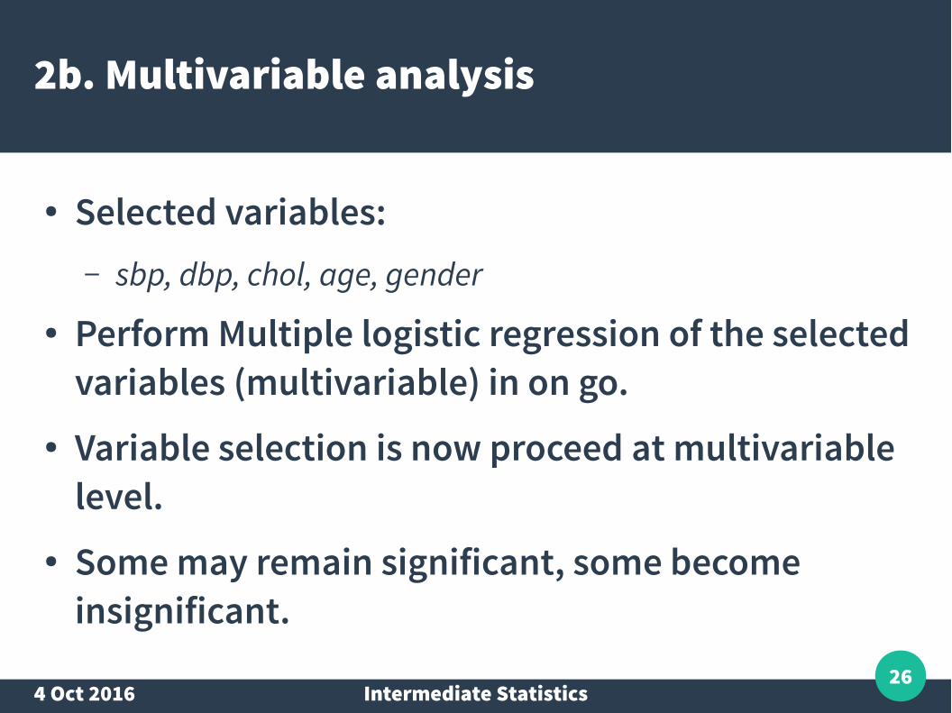
2b. Multivariable analysis
● Selected variables:– sbp, dbp, chol, age, gender
● Perform Multiple logistic regression of the selected variables (multivariable) in on go.
● Variable selection is now proceed at multivariable level.
● Some may remain significant, some become insignificant.
4 Oct 2016 Intermediate Statistics27
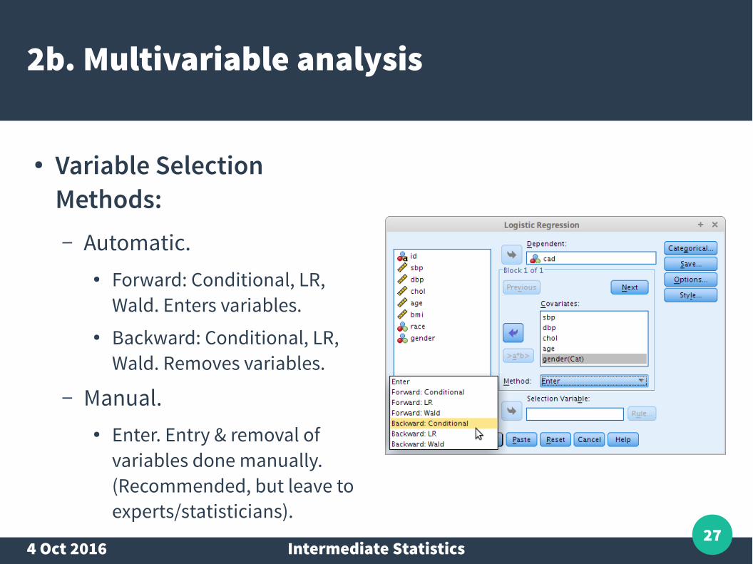
2b. Multivariable analysis
● Variable Selection Methods:– Automatic.
● Forward: Conditional, LR, Wald. Enters variables.
● Backward: Conditional, LR, Wald. Removes variables.
– Manual.● Enter. Entry & removal of
variables done manually. (Recommended, but leave to experts/statisticians).
4 Oct 2016 Intermediate Statistics28
2b. Multivariable analysis
● Variable Selection in this workshop:– Automatic by Forward & Backward LR.– Selection of variables by P-values based on LR test.
4 Oct 2016 Intermediate Statistics29
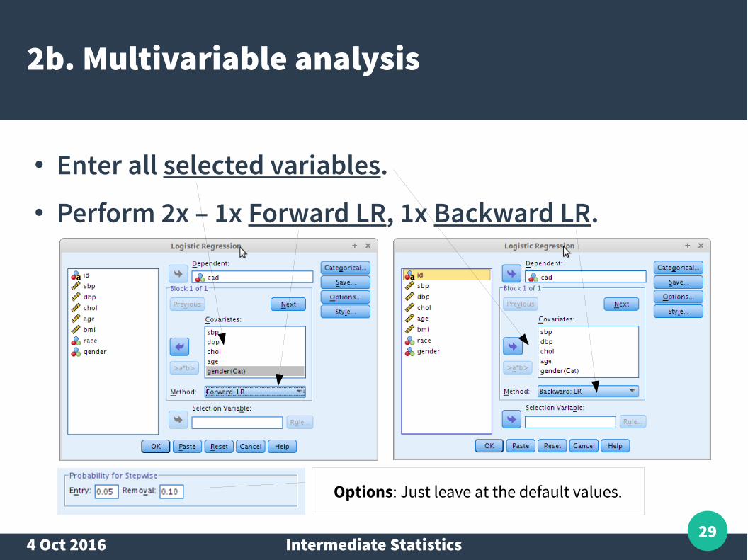
2b. Multivariable analysis
● Enter all selected variables.● Perform 2x – 1x Forward LR, 1x Backward LR.
Options: Just leave at the default values.
4 Oct 2016 Intermediate Statistics30
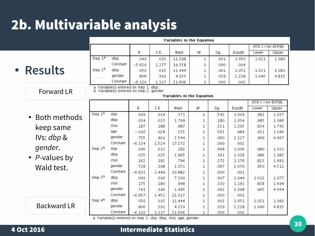
2b. Multivariable analysis
● ResultsForward LR
Backward LR
● Both methods keep same IVs: dbp & gender.
● P-values by Wald test.
4 Oct 2016 Intermediate Statistics31
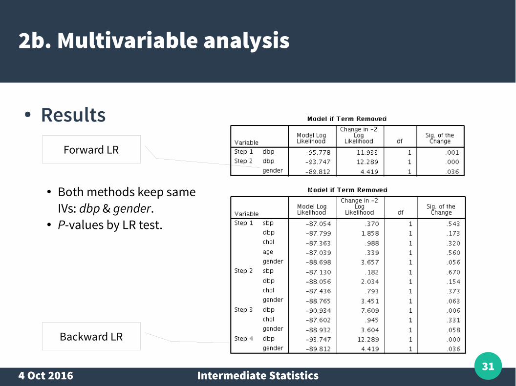
2b. Multivariable analysis
● Results
Backward LR
● Both methods keep same IVs: dbp & gender.
● P-values by LR test.
Forward LR
4 Oct 2016 Intermediate Statistics32
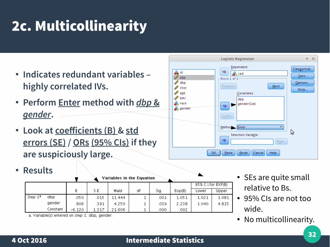
2c. Multicollinearity
● Indicates redundant variables – highly correlated IVs.
● Perform Enter method with dbp & gender.
● Look at coefficients (B) & std errors (SE) / ORs (95% CIs) if they are suspiciously large.
● Results● SEs are quite small
relative to Bs.● 95% CIs are not too
wide.● No multicollinearity.
4 Oct 2016 Intermediate Statistics33
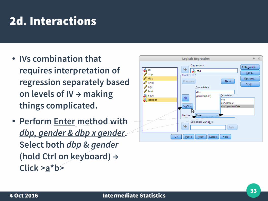
2d. Interactions
● IVs combination that requires interpretation of regression separately based on levels of IV → making things complicated.
● Perform Enter method with dbp, gender & dbp x gender. Select both dbp & gender (hold Ctrl on keyboard) → Click >a*b>
4 Oct 2016 Intermediate Statistics34
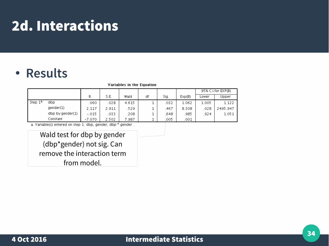
2d. Interactions
● Results
Wald test for dbp by gender (dbp*gender) not sig. Can
remove the interaction term from model.
4 Oct 2016 Intermediate Statistics35
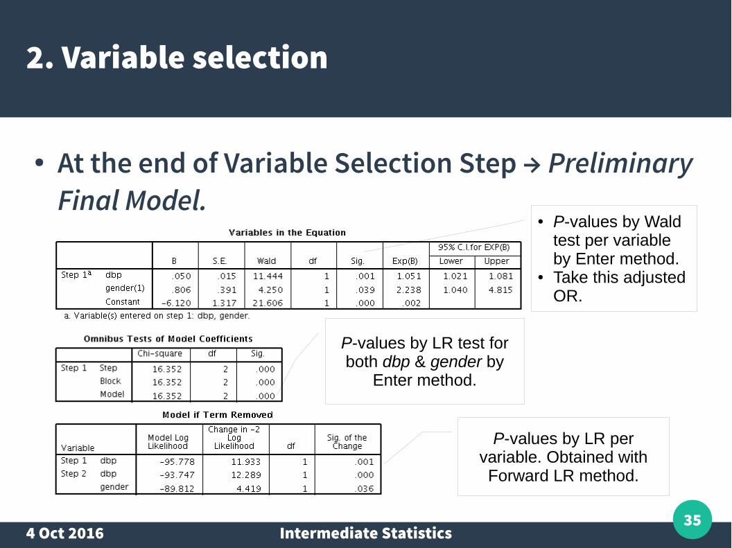
2. Variable selection
● At the end of Variable Selection Step → Preliminary Final Model.
P-values by LR per variable. Obtained with Forward LR method.
● P-values by Wald test per variable by Enter method.
● Take this adjusted OR.
P-values by LR test for both dbp & gender by
Enter method.
4 Oct 2016 Intermediate Statistics36
3. Model fit assessment
● By these 3 goodness-of-fit assessment methods:a. Hosmer-Lemeshow test
b. Classification table.
c. Area under Receiver Operating Characteristics (ROC) curve.
● At the end → Final Model.
4 Oct 2016 Intermediate Statistics37
3. Model fit assessment
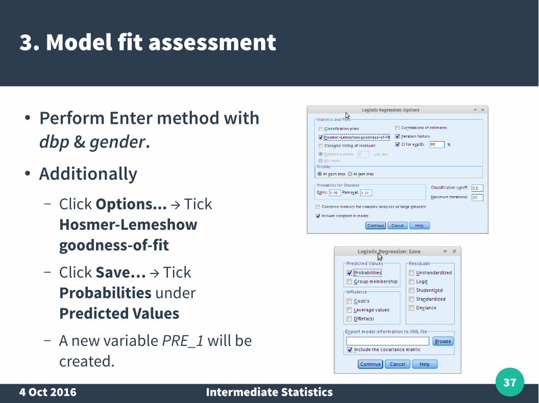
● Perform Enter method with dbp & gender.
● Additionally– Click Options... → Tick
Hosmer-Lemeshow goodness-of-fit
– Click Save… → Tick Probabilities under Predicted Values
– A new variable PRE_1 will be created.
4 Oct 2016 Intermediate Statistics38
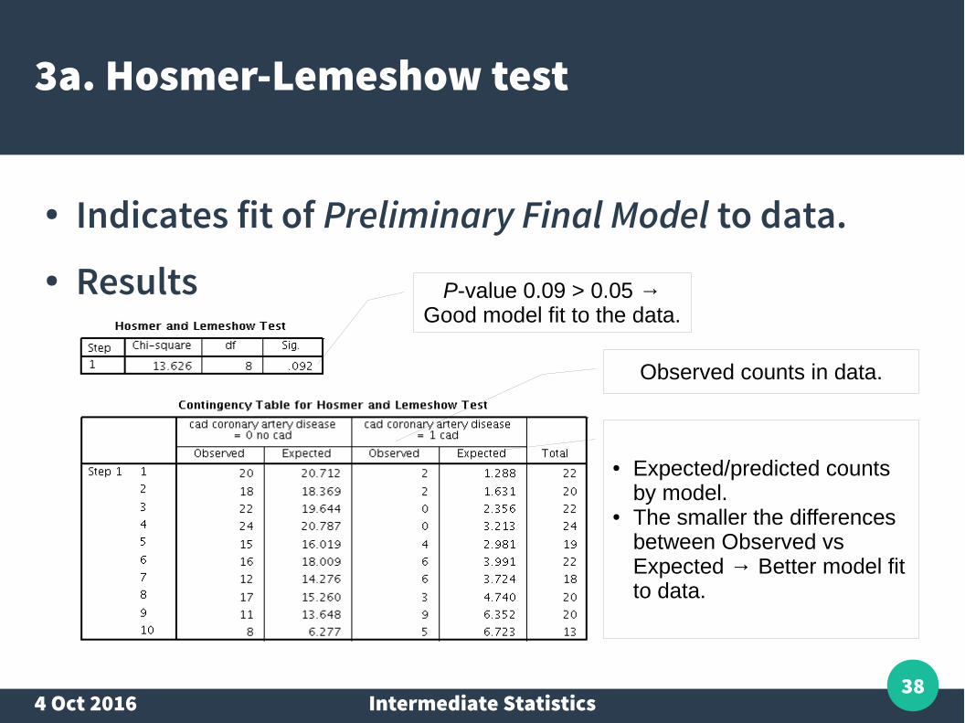
3a. Hosmer-Lemeshow test
● Indicates fit of Preliminary Final Model to data. ● Results P-value 0.09 > 0.05 →
Good model fit to the data.
Observed counts in data.
● Expected/predicted counts by model.
● The smaller the differences between Observed vs Expected → Better model fit to data.
4 Oct 2016 Intermediate Statistics39
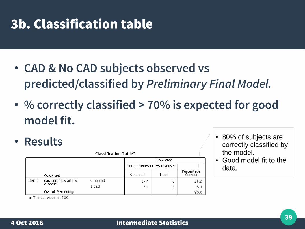
3b. Classification table
● CAD & No CAD subjects observed vs predicted/classified by Preliminary Final Model.
● % correctly classified > 70% is expected for good model fit.
● Results ● 80% of subjects are correctly classified by the model.
● Good model fit to the data.
4 Oct 2016 Intermediate Statistics40
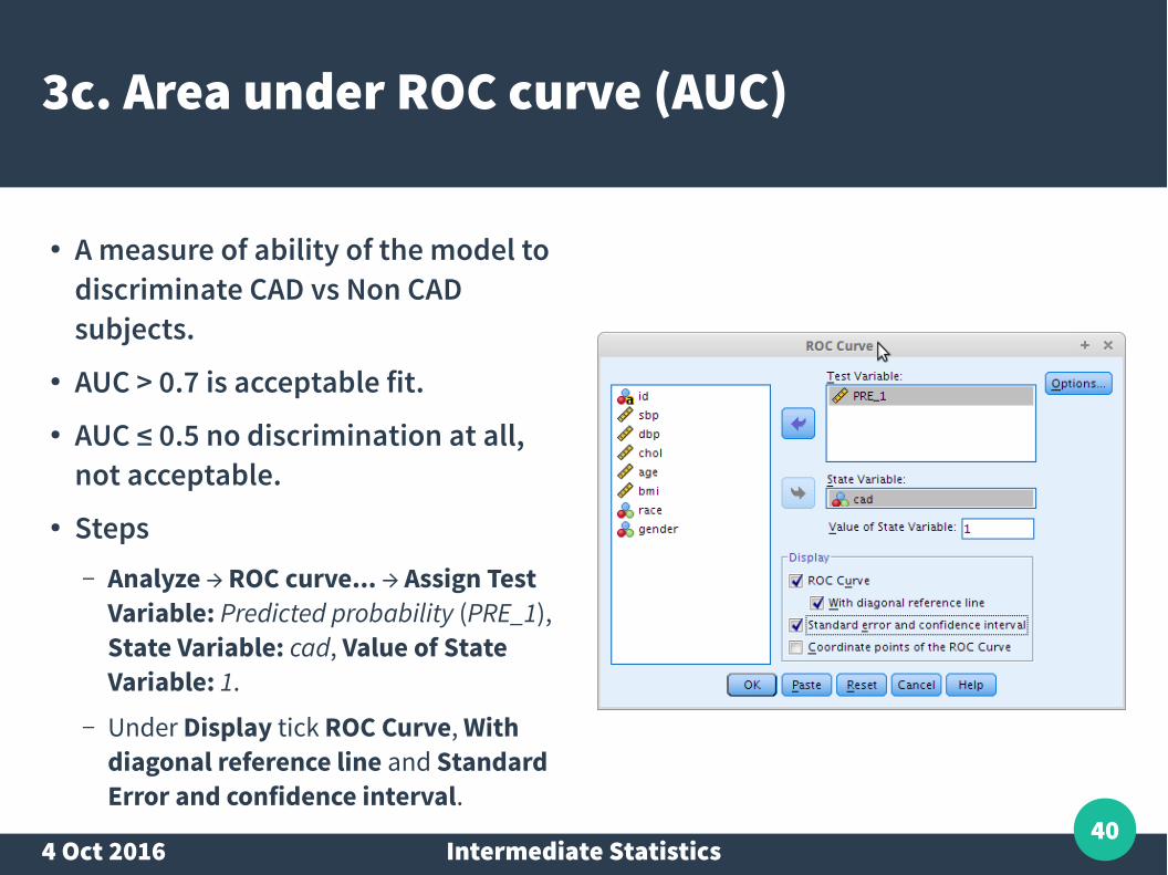
3c. Area under ROC curve (AUC)
● A measure of ability of the model to discriminate CAD vs Non CAD subjects.
● AUC > 0.7 is acceptable fit.● AUC ≤ 0.5 no discrimination at all,
not acceptable.● Steps
– Analyze → ROC curve... → Assign Test Variable: Predicted probability (PRE_1), State Variable: cad, Value of State Variable: 1.
– Under Display tick ROC Curve, With diagonal reference line and Standard Error and confidence interval.
4 Oct 2016 Intermediate Statistics41
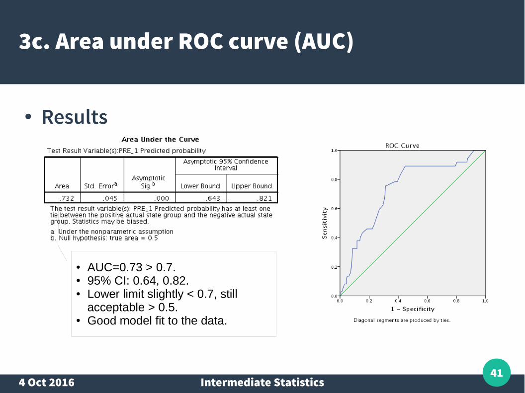
3c. Area under ROC curve (AUC)
● Results
● AUC=0.73 > 0.7.● 95% CI: 0.64, 0.82.● Lower limit slightly < 0.7, still
acceptable > 0.5.● Good model fit to the data.
4 Oct 2016 Intermediate Statistics42
3. Model fit assessment
● All 3 methods indicate good model fit of Preliminary Final Model.
● Can conclude the model with dbp & gender → Final Model.
4 Oct 2016 Intermediate Statistics43
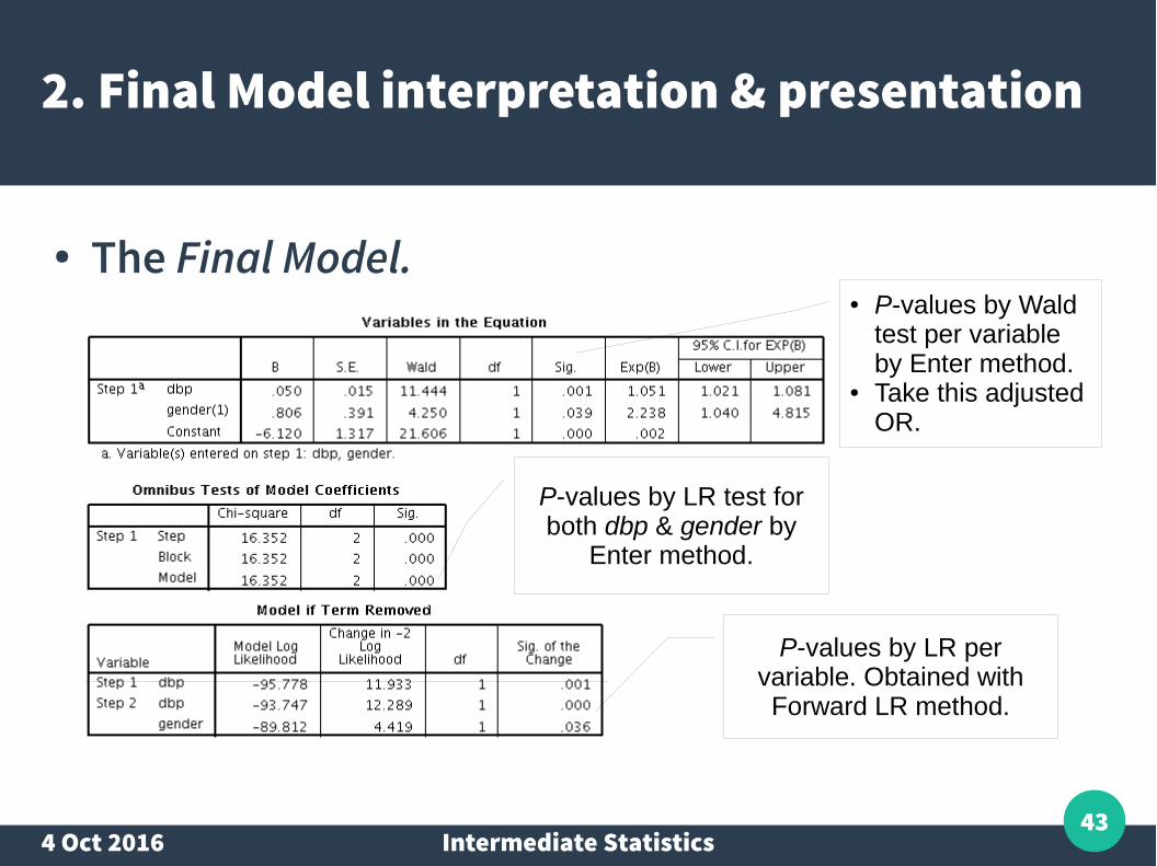
2. Final Model interpretation & presentation
● The Final Model.
P-values by LR per variable. Obtained with Forward LR method.
● P-values by Wald test per variable by Enter method.
● Take this adjusted OR.
P-values by LR test for both dbp & gender by
Enter method.
4 Oct 2016 Intermediate Statistics44
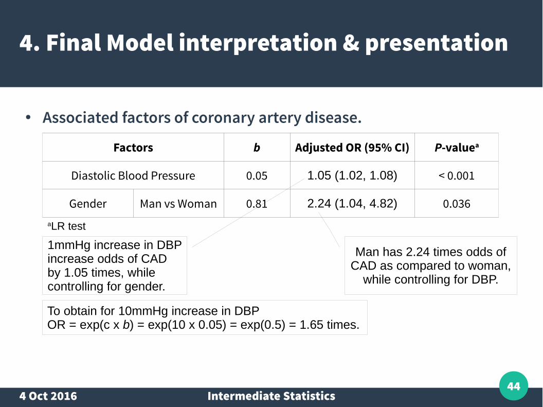
4. Final Model interpretation & presentation
● Associated factors of coronary artery disease.
Factors b Adjusted OR (95% CI) P-valuea
Diastolic Blood Pressure 0.05 1.05 (1.02, 1.08) < 0.001
Gender Man vs Woman 0.81 2.24 (1.04, 4.82) 0.036aLR test
1mmHg increase in DBP increase odds of CAD by 1.05 times, while controlling for gender.
Man has 2.24 times odds of CAD as compared to woman,
while controlling for DBP.
To obtain for 10mmHg increase in DBPOR = exp(c x b) = exp(10 x 0.05) = exp(0.5) = 1.65 times.
4 Oct 2016 Intermediate Statistics45
Q&A