Multiple Linear Regression,General Linear Model, & Generalized Linear Model

With Thanks to My Students in

AMS 572: Data Analysis

1

Outline

1. Introduction to Multiple Linear Regression2. Statistical Inference 3. Topics in Regression Modeling4. Example 5. Variable Selection Methods6. Regression Diagnostic and Strategy for

Building a Model

2

1.Introduction to Multiple Linear

Regression

3

Multiple Linear Regression

Historical Background

• Regression analysis is a statistical methodology to estimate the relationship of a response variable to a set of predictor variables

• Multiple linear regression extends simple linear regression model to the case of two or more predictor variable

• Francis Galton started using the term regression in his biology research• Karl Pearson and Udny Yule extended Galton’s work to the statistical context• Legendre and Gauss developed the method of least squares used in regression analysis• Ronald Fisher developed the maximum likelihood method used in the related statistical inference (test of the significance of regression etc.).

Example:

A multiple regression analysis might show us that the demand of a product varies directly with the change in demographic characteristics (age, income) of a market area.

4

History

Hi, I am Francis Galton (1822/2/16 –1911/1/17).

You guys regard me as the founder of Biostatistics.In my research I found tall parents usual have shorter children; and vice versa. So the height of human being has the tendency to regress to its mean.Yes, It is me who first use the word “regression” for such phenomenon and problems.

I am Adrien-Marie Legendre (1752/9/18 -

1833/1/10).In 1805, I published an article named Nouvelles méthodes pour la détermination des orbites des comètes. In this article, I introduced Method of Least Squares to the world. Yes, I am the first person who published article regarding to method of least squares, which is the earliest form of regression.

Hi, I am Carl Friedrich Gauss (1777/4/30 – 1855/4/23).

I developed the fundamentals of the basis for least-squares analysis in 1795 at the age of eighteen.I published an article called Theoria Motus Corporum Coelestium in Sectionibus Conicis Solem Ambientum in 1809.In 1821, I published another article about least square analysis with further development, called Theoria combinationis observationum erroribus minimis obnoxiae. This article includes Gauss–Markov theorem

HI, I am Karl Pearson.

Hi, again. I am Ronald Aylmer Fisher.

We both developed regression theory after Galton.

Most content in this page comes from Wikipedia

5

Probabilistic Model

1 1 , 1, 2,...,ki i i k i iY x x x i n

iy is the observed value of the random variable (r.v.)iY

1 2, , ,i i ikx x x according to the following model:

Here 0 1, , , k are unknown model parameters, and n is the number of observations.

The random error, , are assumed to be independent r.v.’s with mean 0 and variance i

Thus are independent r.v.’s with mean and variance , where iY i

1 1( ) ki i i k ii E Y x x x

6

2

fixed predictor values

which depends on

2

Fitting the model

• The least squares (LS) method is used to find a line that fits the equation

• Specifically, LS provides estimates of the unknown model parameters,

1 22

0 1 2

1

[ ( ... )]k

n

i i i k i

i

Q y x x x

0 1, , , k Qwhich minimizes, , the sum of squared difference of the

observed values, , and the corresponding points on the line with the same x’siy

• The LS can be found by taking partial derivatives of Q with respect to the

unknown variables and setting them equal to 0. The result

is a set of simultaneous linear equations.

• The resulting solutions, are the least squares (LS)

estimators of , respectively.

• Please note the LS method is non-parametric. That is, no probability

distribution assumptions on Y or ε are needed.

0 1, , , k 0 1

ˆ ˆ ˆ, , , k

0 1, , , k

7

1 1 , 1, 2,...,ki i i k i iY x x x i n

Goodness of Fit of the Model

ˆ ( 1,2, , )i i ie y y i n • To evaluate the goodness of fit of the LS model, we use the residuals

defined by

• are the fitted values:

• An overall measure of the goodness of fit is the error sum of squares (SSE)

ˆiy

1 1ˆ ˆ ˆ ˆˆ ( 1,2,..., )ki i i k iy x x x i n

2

1

min n

ii

Q SSE e

• A few other definition similar to those in simple linear regression:

total sum of squares (SST):2( )iSST y y

regression sum of squares (SSR):

SSR SST SSE

8

• coefficient of multiple determination:

2 1SSR SSE

RSST SST

• • values closer to 1 represent better fits• adding predictor variables never decreases and generally increases

• multiple correlation coefficient (positive square root of ):

20 1R

2R

2R2R R

• only positive square root is used

• R is a measure of the strength of the association between the predictors

(x’s) and the one response variable Y

9

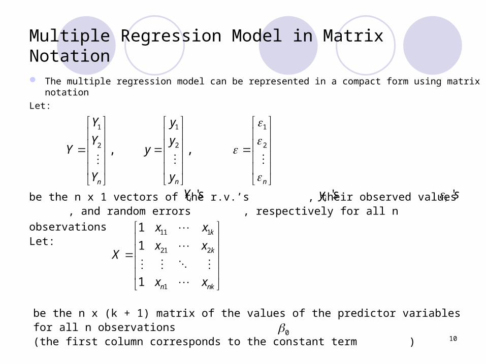
Multiple Regression Model in Matrix Notation

The multiple regression model can be represented in a compact form using matrix notation

Let:

1

2 ,

n

Y

YY

Y

1

2 ,

n

y

yy

y

1

2

n

be the n x 1 vectors of the r.v.’s , their observed values , and random errors ,

respectively for all n observations Let:

'iY s 'iy s 'i s

11 1

21 2

1

1

1

1

k

k

n nk

x x

x xX

x x

be the n x (k + 1) matrix of the values of the predictor variables for all n observations(the first column corresponds to the constant term )

010

Let: 0

1

k

and

0

1

ˆ

ˆˆ

ˆk

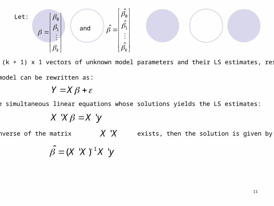
be the (k + 1) x 1 vectors of unknown model parameters and their LS estimates, respectively

• The model can be rewritten as:

Y X • The simultaneous linear equations whose solutions yields the LS estimates:

' 'X X X y • If the inverse of the matrix exists, then the solution is given by:'X X

1ˆ ( ' ) 'X X X y

11

2.Statistical Inference

12

Determining the statistical significance of the predictor variables:

• We test the hypotheses:

H0 j : j 0

H1 j : j 0

• If we can’t reject

H0 j : Bj 0

vs.

, then the corresponding variable

x j is not a significant predictor of y.

• It is easily shown that each j is normal with mean

j

and variance

2v jj , where is the jth diagonal entry of the

matrix

V (X ' X) 1

v jj

13

• For statistical inferences, we need the assumption that

2~ 0,iid

i N *i.i.d. means independent & identically distributed

Deriving a pivotal quantity for the inference on

),(~ˆ 2jjjj vN • Recall

• The unbiased estimator of the unknown error variance

is given by

2

S2 SSE

n (k 1)

ei2

n (k 1)

MSE

d.o. f .

• We also know that2

2( 1)2 2

( ( 1))~ n k

n k S SSEW

, and that

S2and j are statistically independent.

• Withˆ

~ (0,1),j j

jj

Z Nv

and by the definition of the t-distribution,

( 1)

ˆ~

/ ( 1)j j

n k

jj

ZT T

W n k S v

14

we obtain the pivotal quantity for the inference on j

j

Derivation of the Confidence Interval for

j

1)ˆ

( )1(,2/)1(,2/ kn

jj

jjkn t

vStP

1)ˆˆ( )1(,2/)1(,2/ jjknjjjjknj vstvstP

/ 2, ( 1)ˆ ˆ( )j n k jt SE

wherejjj vsSE )ˆ(

15

Thus the 100(1-α)% confidence interval for is:

j

Derivation of the Hypothesis Test for at the significance level αHypotheses: 0 : 0

: 0

j

a j

H

H

P (Reject H0 | H0 is true) =

/ 2, ( 1)n kc t

Therefore, we reject H0 at the significance level α if and only if , where is the observed value of 0 / 2, ( 1)n kt t

16

The test statistic is: 0

0 ( 1)

ˆ 0~H

jn k

jj

T TS v

The decision rule of the test is derived based on the Type I error rate α. That is

0( )P T c

0t 0T

j

Another Hypothesis Test

Now consider:for all

for at least one

When H0 is true, the test statistics

• An alternative and equivalent way to make a decision for a statistical test is through the p-value, defined as:

p = P(observe a test statistic value at least as extreme as the one observed

• At the significance level , we reject H0 if and only if p <

H0 : j 0

Ha : j 0

0 j k

0 j k

0 , ( 1)~ k n k

MSRF f

MSE

17

0| )H

The General Hypothesis Test

• Consider the full model:

• Now consider a partial model:

• Test statistic:

• Reject H0 when

Yi 0 1x i1 ...k x ik i (i=1,2,…n)

Yi 0 1x i1 ...k m x i,k m i

0 , ( 1)

( ) /~

/[ ( 1)]k m k

m n kk

SSE SSE mF f

SSE n k

H0 :k m1 ...k 0 vs.

Ha : j 0

for at least one

k m 1 j k

0 , ( 1),m n kF f

(i=1,2,…n)

• Hypotheses:

18

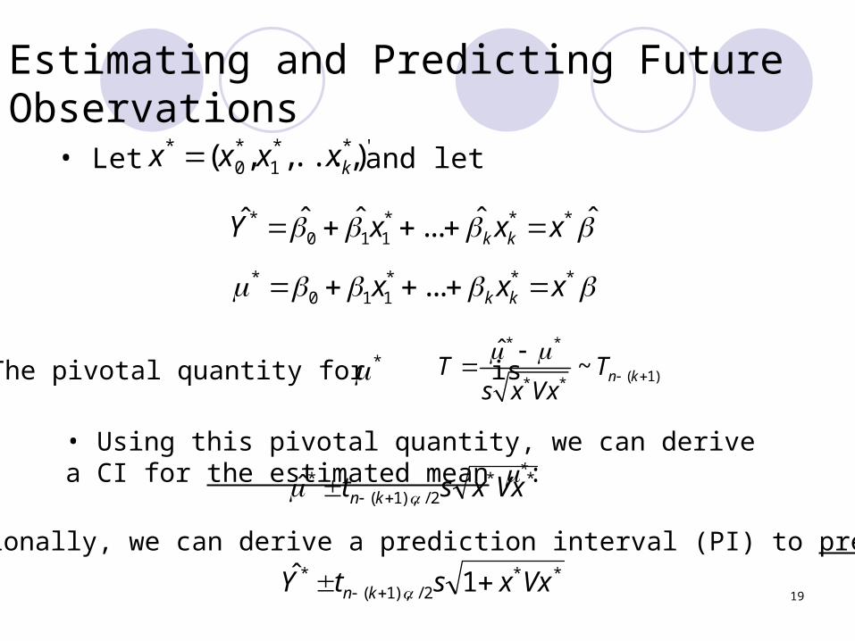
Estimating and Predicting Future Observations

• Let

x* (x0*,x1

*,...,xk*)'

* * * * 0 1 1

ˆ ˆ ˆ ˆˆ ... k kY x x x

• The pivotal quantity for is* *

( 1)* *

ˆ~ n kT T

s x Vx

• Using this pivotal quantity, we can derive a CI for the estimated mean *: * *

2/),1(*ˆ Vxxst kn

• Additionally, we can derive a prediction interval (PI) to predict Y*:* *

2/),1(* 1ˆ VxxstY kn

and let

19

* * * * 0 1 1 ... k kx x x

*

3. Topics in Regression

Modeling

20

3.1 Multicollinearity

Definition. The predictor variables are linearly dependent.

This can cause serious numerical and statistical difficulties in fitting the regression model unless “extra” predictor variables are deleted.

21

How does the multicollinearity cause difficulties?

.computable and unique be to for order in

invertable be must Thus , equation the to solution the is ^

^

XXyXXX TTT

If the approximate multicollinearity happens:

1. is nearly singular, which makes numerically unstable. This reflected in large changes in their magnitudes with small changes in data.

2. The matrix has very large elements. Therefore are large, which makes statistically nonsignificant.

TX X^

1)( XXV TjjvVar 2

^

)( j

^

22

Measures of Multicollinearity

1. The correlation matrix R.Easy but can’t reflect linear relationships between more than two variables.

2. Determinant of R can be used as measurement of singularity of .

3. Variance Inflation Factors (VIF): the diagonal elements of . VIF>10 is regarded as unacceptable.

TX X

1R

23

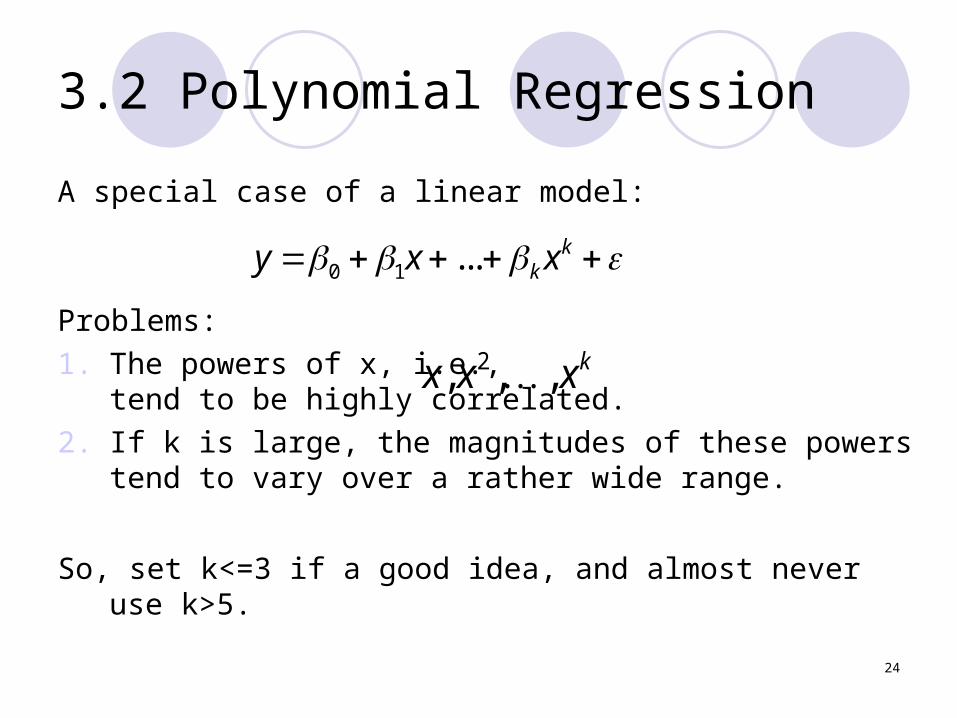
3.2 Polynomial Regression

A special case of a linear model:

Problems:

1. The powers of x, i.e., tend to be highly correlated.

2. If k is large, the magnitudes of these powers tend to vary over a rather wide range.

So, set k<=3 if a good idea, and almost never use k>5.

0 1 ... kky x x

2, , , kx x x

24

Solutions1. Centering the x-variable:

Effect: removing the non-essential multicollinearity in the data.

2. Further more, we can standardize the data by dividing the standard deviation of x:

Effect: helping to alleviate the second problem.

3. Using the first few principal components of the original variables instead of the original variables.

* * *0 1 ( ) ... ( )k

ky x x x x

x

x x

s

xs

25

3.3 Dummy Predictor Variables & The General Linear Model

How to handle the categorical predictor variables?

1. If we have categories of an ordinal variable, such as the prognosis of a patient (poor, average, good), one can assign numerical scores to the categories. (poor=1, average=2, good=3)

26

2. If we have nominal variable with c>=2 categories. Use c-1 indicator variables, , called Dummy Variables, to code.

for the ith category,

for the cth category.

1 1, , cx x

1ix 1 1i c

1 1... 0cx x

27

Why don’t we just use c indicator variables:

?

If we use that, there will be a linear dependency among them:

This will cause multicollinearity.

1 2, ,..., cx x x

1 2 ... 1cx x x

28

Example of the dummy variables

For instance, if we have four years of quarterly sale data of a certain brand of soda. How can we model the time trend by fitting a multiple regression equation?

Solution: We use quarter as a predictor variable x1. To model the seasonal trend, we use indicator variables x2, x3, x4, for Winter, Spring and Summer, respectively. For Fall, all three equal zero. That means: Winter-(1,0,0), Spring-(0,1,0), Summer-(0,0,1), Fall-(0,0,0).

Then we have the model:0 1 1 2 2 3 3 4 4 ( 1,...,16)i i i i i iY x x x x i

29

3. Once the dummy variables are included, the resulting regression model is referred to as a “General Linear Model”.

This term must be differentiated from that of the “Generalized Linear Model” which include the “General Linear Model” as a special case with the identity link function:

The generalized linear model will link the model parameters to the predictors through a link function. For another example, we will check out the logit link in the logistic regression this afternoon.

30

1 1( ) ki i i k ii E Y x x x

Another Example of Generalized Linear Model:

Logistic Regression Model In 1938, Ronald

Fisher and Frank Yates suggested the logit link for regression with a binary response variable.

0 1

( 1| ) ( 1| )ln ln

( 0 | ) 1 ( 1| )

ln1

P Y x P Y x

P Y x P Y x

xx

x

ln(Odds of Y 1| x)

A popular model for categorical response variable

Logistic regression model is perhaps the most popular generalized linear model for binary data.

Logistic regression model is generally used to study the relationship between a binary response variable and a group of predictors (can be either continuous or categorical).

Y = 1 (true, success, YES, etc.) or

Y = 0 ( false, failure, NO, etc.)Logistic regression model can be extended to model a

categorical response variable with more than two categories. The resulting model is sometimes referred to as the multinomial logistic regression model (in contrast to the ‘binomial’ logistic regression for a binary response variable.)

More on the rationale of the logistic regression model

Consider a binary response variable Y=0 or 1and a single predictor variable x. We want to model E(Y|x) =P(Y=1|x) as a function of x. The logistic regression model expresses the logistic transform of P(Y=1|x) as a linear function of the predictor.

This model can be rewritten as

E(Y|x)= P(Y=1| x) *1 + P(Y=0|x) * 0 = P(Y=1|x) is bounded between 0 and 1 for all values of x. The following linear model may violate this condition sometimes:

P(Y=1|x) =

0 1

( 1| )ln

1 ( 1| )

P Y xx

P Y x

)exp(1

)exp()|1(

10

10

x

xxYP

x10

More on the properties of the logistic regression model

In the simple logistic regression, the regression coefficient has the interpretation that it is the log of the odds ratio of a success event (Y=1) for a unit change in x.

For multiple predictor variables, the logistic regression model is

1

11010 ][)]1([)|0(

)|1(ln

)1|0(

)1|1(ln

xxxYP

xYP

xYP

xYP

kkk

k xxxxxYP

xxxYP

...),...,,|0(

),...,,|1(ln 110

21

21

Logistic Regression, SAS Procedure http://www.ats.ucla.edu/stat/sas/output/SAS_logit_output.htm Proc Logistic This page shows an example of logistic regression with footnotes explaining the output.

The data were collected on 200 high school students, with measurements on various tests, including science, math, reading and social studies. The response variable is high writing test score (honcomp), where a writing score greater than or equal to 60 is considered high, and less than 60 considered low; from which we explore its relationship with gender (female), reading test score (read), and science test score (science). The dataset used in this page can be downloaded from http://www.ats.ucla.edu/stat/sas/webbooks/reg/default.htm.

data logit; set "c:\temp\hsb2";

honcomp = (write >= 60);

run;

proc logistic data= logit descending;

model honcomp = female read science;

run;

35

Logistic Regression, SAS Output

36

4. Example(Now we are back to General Linear Model) Here we revisit the classic regression towards

Mediocrity in Hereditary Stature by Francis Galton He performed a simple regression to predict offspring

height based on the average parent height Slope of regression line was less than 1 showing that

extremely tall parents had less extremely tall children At the time, Galton did not have multiple regression as

a tool so he had to use other methods to account for the difference between male and female heights

We can now perform multiple regression on parent-offspring height and use multiple variables as predictors

37

Example

Y = height of child x1 = height of father x2 = height of mother x3 = gender of child

iiiioi xxxY 332211

38

Example

We find that: β0 = 15.34476 β1 = 0.405978 β2 = 0.321495 β3 = 5.22595

In matrix notation:

yXXX

XY

')'( 1

39

ExampleFather Mother Gender Child

1 78.5 67 1 73.2

1 78.5 67 1 69.2

1 78.5 67 0 69

1 78.5 67 0 69

1 75.5 66.5 1 73.5

1 75.5 66.5 1 72.5

1 75.5 66.5 0 65.5

1 75.5 66.5 0 65.5

1 75 64 1 71

1 75 64 0 68

… … … … …

X

40

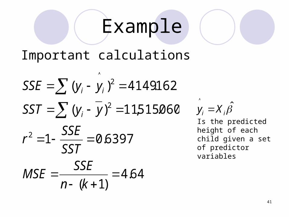
Example

64.4)1(

6397.01

060.515,11)(

162.4149)(

2

2

2

kn

SSEMSE

SST

SSEr

yySST

yySSE

i

ii

Is the predicted height of each child given a set of predictor variables

ˆi iy X

Important calculations

41

Example

Ho: βj = 0

Ha: βj ≠ 0

Reject H0j if ( 1), /2 894,0.025

1

2.245( )

1.63 0.0118 0.0125 0.00596

0.0118 0.000184 0.0000143 0.0000223( ' )

0.0125 0.0000143 0.000211 0.0000327

0.00596 0.0000223 0.0000327 0.00447

( )

j

j n k

j

j

t t tSE

V X X

SE

* jjMSE v

Are these values significantly different than zero?

42

Exampleβ-estimate SE t

Intercept 15.3 2.75 5.59*

Father Height

0.406 0.0292 13.9*

Mother Height

0.321 0.0313 10.3*

Gender 5.23 0.144 36.3** p<0.05. We conclude that all β are significantly different than zero. 43

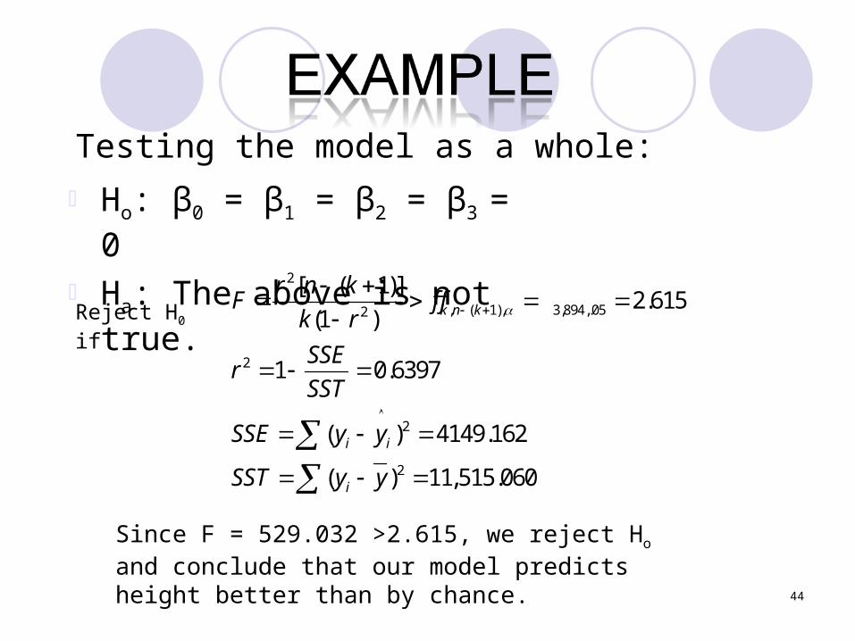
Ho: β0 = β1 = β2 = β3 = 0

Ha: The above is not true.2

, ( 1), 3,894,.052

2

2

2

[ ( 1)]2.615

(1 )

1 0.6397

( ) 4149.162

( ) 11,515.060

k n k

i i

i

r n kF f f

k r

SSEr

SST

SSE y y

SST y y

Reject H0 if

Since F = 529.032 >2.615, we reject Ho and conclude that our model predicts height better than by chance.

Testing the model as a whole:

44

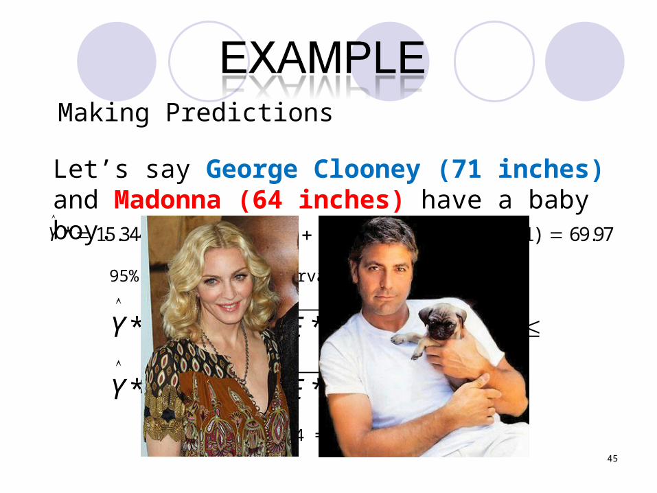
*)*'1(**

**)*'1(**

025,.894

025,.894

VxxMSEtY

YVxxMSEtY

Let’s say George Clooney (71 inches) and Madonna (64 inches) have a baby boy.

* 15.34476 0.405978 (71) 0.321495(64) + 5.225951(1) 69.97Y

95% Prediction interval:

69.97 ± 4.84 = (65.13, 74.81)

Making Predictions

45

ods graphics ondata revise; set mylib.galton; if sex = 'M' then gender = 1.0; else gender = 0.0;run;

proc reg data=revise;title "Dependence of Child Heights on Parental

Heights";model height = father mother gender / vif;run;quit;

Alternatively, one can use proc GLM procedure that can incorporate the categorical variable (sex) directly via the class statement.

SAS code

46

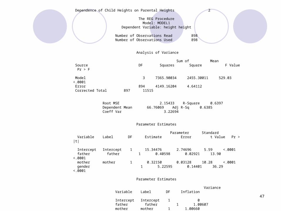
Dependence of Child Heights on Parental Heights 2

The REG Procedure Model: MODEL1 Dependent Variable: height height

Number of Observations Read 898 Number of Observations Used 898

Analysis of Variance

Sum of Mean Source DF Squares Square F Value Pr > F

Model 3 7365.90034 2455.30011 529.03 <.0001 Error 894 4149.16204 4.64112 Corrected Total 897 11515

Root MSE 2.15433 R-Square 0.6397 Dependent Mean 66.76069 Adj R-Sq 0.6385 Coeff Var 3.22694

Parameter Estimates

Parameter Standard Variable Label DF Estimate Error t Value Pr > |t|

Intercept Intercept 1 15.34476 2.74696 5.59 <.0001 father father 1 0.40598 0.02921 13.90 <.0001 mother mother 1 0.32150 0.03128 10.28 <.0001 gender 1 5.22595 0.14401 36.29 <.0001

Parameter Estimates

Variance Variable Label DF Inflation

Intercept Intercept 1 0 father father 1 1.00607 mother mother 1 1.00660 gender 1 1.00188

47

48

By Gary Bedford &Christine Vendikos 49

5. Variables Selection Method

A. Stepwise Regression

50

Variables selection method

(1) Why do we need to select the variables?

(2) How do we select variables?

* stepwise regression

* best subset regression

51

Stepwise Regression

(p-1)-variable model:

P-variable model

ipipii xxY 1,11,10 ...

ipippipii xxxY ,1,11,10 ...

52

0

0

testHypothesis

test-F Partial

:1

:0

pp

pp

H

H

2/),1(0

),1(,11

|:|

)(:

)]1(/[

1/)(

pnpp

p

pp

pnp

ppp

ttHreject

SEtstatistictest

fpnSSE

SSESSEF

53

Partial correlation coefficients

2

2

2

11

1111|

2

1...1|

1...1|

1...1

1

)]1([

)...(

)...()...(

pxxpyx

pxxpyx

pp

r

pnrtF

xxSSE

xxSSExxSSE

SSE

SSESSEr

pp

p

pp

p

ppxxyx

54

5. Variables selection method

A. Stepwise Regression:

SAS Example

55

No. X1 X2 X3 X4 Y

1 7 26 6 60 78.5

2 1 29 15 52 74.3

3 11 56 8 20 104.3

4 11 31 8 47 87.6

5 7 52 6 33 95.9

6 11 55 9 22 109.2

7 3 71 17 6 102.7

8 1 31 22 44 72.5

9 2 54 18 22 93.1

10 21 47 4 26 1159

11 1 40 23 34 83.8

12 11 66 9 12 113.3

13 10 68 8 12 109.4

Example 11.5 (T&D pg. 416), 11.9 (T&D pg. 431)

The following table shows data on the heat evolved in calories during the hardening of cement on a per gram basis (y) along with the percentages of four ingredients: tricalcium aluminate (x1), tricalcium silicate (x2), tetracalcium alumino ferrite (x3), and dicalcium silicate (x4).

56

SAS Program (stepwise variable selection is used)

data example115;input x1 x2 x3 x4 y;datalines; 7 26 6 60 78.5 1 29 15 52 74.311 56 8 20 104.311 31 8 47 87.6 7 52 6 33 95.911 55 9 22 109.2 3 71 17 6 102.7 1 31 22 44 72.5 2 54 18 22 93.121 47 4 26 115.9 1 40 23 34 83.811 66 9 12 113.310 68 8 12 109.4;run;proc reg data=example115; model y = x1 x2 x3 x4 /selection=stepwise;run; 57

Selected SAS output

The SAS System 22:10 Monday, November 26, 2006 3

The REG Procedure Model: MODEL1 Dependent Variable: y

Stepwise Selection: Step 4

Parameter StandardVariable Estimate Error Type II SS F Value Pr > F

Intercept 52.57735 2.28617 3062.60416 528.91 <.0001x1 1.46831 0.12130 848.43186 146.52 <.0001x2 0.66225 0.04585 1207.78227 208.58 <.0001

Bounds on condition number: 1.0551, 4.2205----------------------------------------------------------------------------------------------------

58

SAS Output (cont)

All variables left in the model are significant at the 0.1500 level.

No other variable met the 0.1500 significance level for entry into the model.

Summary of Stepwise Selection

Variable Variable Number Partial Model Step Entered Removed Vars In R-Square R-Square C(p) F Value Pr > F

1 x4 1 0.6745 0.6745 138.731 22.80 0.0006 2 x1 2 0.2979 0.9725 5.4959 108.22 <.0001 3 x2 3 0.0099 0.9823 3.0182 5.03 0.0517 4 x4 2 0.0037 0.9787 2.6782 1.86 0.2054

59

5. Variables selection method

B. Best Subsets Regression

60

Best Subsets Regression

For the stepwise regression algorithmThe final model is not guaranteed to be optimal

in any specified sense.

In the best subsets regression, subset of variables is chosen from the collection

of all subsets of k predictor variables) that optimizes a well-defined objective criterion

61

Best Subsets Regression

In the stepwise regression,We get only one single final models.

In the best subsets regression, The investor could specify a size for the

predictors for the model.

62

Best Subsets Regression

SST

SSE

SST

SSRr pp

p 12

Optimality Criteria

• rp2-Criterion:

n

iiipp YEYE

1

22

]][]ˆ[[1

The sample estimator, Mallows’ Cp-statistic, is given by

• Cp-Criterion (recommended for its ease of computation and its ability

to judge the predictive power of a model)

npSSE

C pp )1(2

ˆ 2

• Adjusted rp2-Criterion:

MST

MSEr p

padj 12,

63

Best Subsets Regression

AlgorithmNote that our problem is to find the minimum of a given function.

Use the stepwise subsets regression algorithm and replace the partial F criterion with other criterion such as Cp.

Enumerate all possible cases and find the minimum of the criterion functions.

Other possibility?

64

Best Subsets Regression & SAS

proc reg data=example115;

model y = x1 x2 x3 x4 /selection=ADJRSQ;

run;

For the selection option, SAS has implemented 9 methods in total. For best subset method, we have the following options:

Maximum R2 Improvement (MAXR) Minimum R2 (MINR) Improvement R2 Selection (RSQUARE) Adjusted R2 Selection (ADJRSQ) Mallows' Cp Selection (CP)

65

6. Building A Multiple Regression Model

Steps and Strategy

66

Modeling is an iterative process. Several cycles of the steps maybe needed before arriving at the final model.

The basic process consists of seven steps

67

Get started and Follow the Steps

Categorization by Usage Collect the Data

Divide the Data Explore the Data

Fit Candidate Models

Select and Evaluate

Select the Final Model

68

Step I

Decide the type of model needed, according to different usage.

Main categories include: Predictive Theoretical Control Inferential Data Summary

• Sometimes, models are involved in multiple purposes.

69

Step II

Collect the Data

Predictor (X)

Response (Y)

Data should be relevant and bias-free

70

Step III

Explore the Data

Linear Regression Model is sensitive to the noise. Thus, we should treat outliers and influential observations cautiously.

71

Step IV

Divide the Data

Training Sets: building

Test Sets: checking

How to divide? Large sample Half-Half

Small sample size of training set >16

72

Step V

Fit several Candidate Models

Using Training Set.

73

Step VI

Select and Evaluate a Good Model To improve the violations of model assumptions.

74

Step VII

Select the Final Model

Use test set to compare competing models by cross-validating them.

75

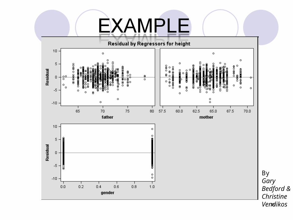
Regression Diagnostics (Step VI)

Graphical Analysis of ResidualsPlot Estimated Errors vs. Xi ValuesDifference Between Actual Yi & Predicted Yi

Estimated Errors Are Called Residuals

Plot Histogram or Stem-&-Leaf of Residuals

PurposesExamine Functional Form (Linearity )Evaluate Violations of Assumptions

76

Linear Regression Assumptions

Mean of Probability Distribution of Error Is 0

Probability Distribution of Error Has Constant Variance

Probability Distribution of Error is NormalErrors Are Independent

77

Residual Plot for Functional Form (Linearity)

X

e

X

e

Add X^2 TermAdd X^2 Term Correct SpecificationCorrect Specification

78

Residual Plot for Equal Variance

X

SR

X

SR

Unequal VarianceUnequal Variance Correct SpecificationCorrect Specification

Fan-shaped.Fan-shaped.Standardized residuals used typically (residual Standardized residuals used typically (residual

divided by standard error of prediction)divided by standard error of prediction) 79

Residual Plot for Independence

X

SR

X

SR

Not IndependentNot Independent Correct SpecificationCorrect Specification

80

Questions?

www.ams.sunysb.edu/~zhu

zhu@ams.sunysb.edu

81