Multiple Imputation with Diagnostics (mi) in R: …gelman/research/published/mipaper...We have...
27
JSS Journal of Statistical Software MMMMMM YYYY, Volume VV, Issue II. http://www.jstatsoft.org/ Multiple Imputation with Diagnostics (mi) in R: Opening Windows into the Black Box Yu-Sung Su Columbia University and New York University Andrew Gelman Columbia University Jennifer Hill New York University Masanao Yajima University of California at Los Angeles Abstract Our mi package in R has several features that allow the user to get inside the impu- tation process and evaluate the reasonableness of the resulting models and imputations. These features include: flexible choice of predictors, models, and transformations for chained imputation models; binned residual plots for checking the fit of the conditional distributions used for imputation; and plots for comparing the distributions of observed and imputed data in one and two dimensions. In addition, we use Bayesian models and weakly informative prior distributions to construct more stable estimates of imputation models. Our goal is to have a demonstration package that (a) avoids many of the practical problems that arise with existing multivariate imputation programs, and (b) demonstrates state-of-the-art diagnostics that can be applied more generally and can be incorporated into the software of the others. Keywords : multiple imputation, model diagnostics, chained equations, weakly informative prior, mi, R. 1. Introduction The general statistical theory and framework for managing missing information has been well developed since Rubin (1987) published his pioneering treatment of multiple imputation meth- ods for nonresponse in surveys. Several software packages have been developed to implement these methods to deal with incomplete datasets. However, each of these imputation packages is, to a certain degree, a black box, and the user must trust the imputation procedure without much control over what goes into it and without much understanding of what comes out. Model checking and other diagnostics are generally an important part of any statistical pro-
Transcript of Multiple Imputation with Diagnostics (mi) in R: …gelman/research/published/mipaper...We have...
JSS Journal of Statistical SoftwareMMMMMM YYYY Volume VV Issue II httpwwwjstatsoftorg
Multiple Imputation with Diagnostics (mi) in R
Opening Windows into the Black Box
Yu-Sung SuColumbia University
andNew York University
Andrew GelmanColumbia University
Jennifer HillNew York University
Masanao YajimaUniversity of California
at Los Angeles
Abstract
Our mi package in R has several features that allow the user to get inside the impu-tation process and evaluate the reasonableness of the resulting models and imputationsThese features include flexible choice of predictors models and transformations forchained imputation models binned residual plots for checking the fit of the conditionaldistributions used for imputation and plots for comparing the distributions of observedand imputed data in one and two dimensions In addition we use Bayesian models andweakly informative prior distributions to construct more stable estimates of imputationmodels Our goal is to have a demonstration package that (a) avoids many of the practicalproblems that arise with existing multivariate imputation programs and (b) demonstratesstate-of-the-art diagnostics that can be applied more generally and can be incorporatedinto the software of the others
Keywords multiple imputation model diagnostics chained equations weakly informativeprior mi R
1 Introduction
The general statistical theory and framework for managing missing information has been welldeveloped since Rubin (1987) published his pioneering treatment of multiple imputation meth-ods for nonresponse in surveys Several software packages have been developed to implementthese methods to deal with incomplete datasets However each of these imputation packagesis to a certain degree a black box and the user must trust the imputation procedure withoutmuch control over what goes into it and without much understanding of what comes out
Model checking and other diagnostics are generally an important part of any statistical pro-
2 mi Multiple Imputation with Diagnostics in R
cedure Examining the implications of imputations is particularly important because of theinherent tension of multiple imputation that the model used for the imputations is not ingeneral the same as the model used for the analysis (Meng 1994 Fay 1996 Robins and Wang2000) We have created an open-ended open source mi package not only to solve theseimputation problems but also to develop and implement new ideas in modeling and modelcheckingOur mi package in R (R Development Core Team 2009) has several features that allow theuser to get inside the imputation process and evaluate the reasonableness of the resultingmodel and imputations These features include flexible choice of predictors models andtransformations for chained imputation models binned residual plots for checking the fit ofthe conditional distributions used for imputation and plots for comparing the distributionsof observed and imputed data in one and two dimensions mi uses an algorithm known asa chained equation approach (van Buuren and Oudshoorn 2000 Raghunathan LepkowskiVan Hoewyk and Solenberger 2001) the user specifies the conditional distribution of eachvariable with missing values conditioned on other variables in the data and the imputationalgorithm sequentially iterates through the variables to impute the missing values using thespecified modelThis article will spare readers from reading through the theoretical background of multipleimputation (Little and Rubin 2002 Gelman and Hill 2007 chapter 25) Rather the majorgoal is to demonstrate the way in which the users can perform multiple imputation with miand to introduce functions for diagnostics after imputation The paper proceeds as followsIn Section 2 we provide a simplified overview of steps to do sensible multiple imputation InSection 3 we demonstrate some novel features and functions of mi that solve some imputationproblems that have not been addressed by other software These features include (1) Bayesianregression models to address problems with separation (2) imputation steps that deal withsemi-continuous data (3) modeling strategies that handle issues of perfect correlation andstructural correlation (4) functions that check the convergence of the imputations and (5)plotting functions that visually check the imputation models In Section 4 we demonstratehow to apply these functions using an example of a study of people living with HIV in NewYork City (Messeri Lee Abramson Aidala Chiasson and Jessop 2003) In Section 5 wediscuss some loose ends and future plans for our mi package
2 Basic Setup of mi
The procedure to obtain sensible multiply imputed datasets approach requires roughly foursteps setup imputation analysis and validation Each step is divided into substeps asfollows
1 Setup
Display of missing data patterns Identifying structural problems in the data and preprocessing Specifying the conditional models
2 Imputation
Iterative imputation based on the conditional model
Journal of Statistical Software 3
Checking the fit of conditional models
Checking the convergence of the procedure
Checking to see if the imputed values are reasonable
3 Analysis
Obtaining completed data
Pooling the complete case analysis on multiply imputed datasets
4 Validation
Sensitivity analysis
Cross validation
At first glance it may seem more complicated to conduct multiple imputation using mi be-cause we outline steps that other packages ignore However in Section 4 we will demonstratethe way in which users can easily implement these imputation steps using mi via an exam-ple mi is designed for both novice and experienced users For the novice users mi has astep-by-step interactive interface where users choose options from the given multiple choices(see Section 46) For more experienced users mi has simple commands that users can use toconduct a multiple imputation
The implementation of the mi package is straightforward The core function is a genericfunction mi(object ) which implements one of two methods depending on whether theinput is of the the dataframe class or the S4 class mi The mi class defines the outputreturned by mi() when it finishes a multiple imputation with a dataset The usages of thetwo methods are described below
S4 method for signature dataframemi(object info nimp = 3 niter = 30
Rhat = 11 maxminutes = 20 randimpmethod = bootstrappreprocess = TRUE runpastconvergence = FALSEseed = NA checkcoefconvergence = FALSEaddnoise = noisecontrol() postrun = TRUE)
S4 method for signature mimi(object info niter = 30 Rhat = 11
maxminutes = 20 randimpmethod = bootstraprunpastconvergence = FALSE seed = NA)
object A data frame or an mi object that contains an incomplete data mi identifiesNArsquos as the missing data
info The miinfo object (see Section 21)
nimp The number of multiple imputations Default is 3 chains
niter The maximum number of imputation iterations Default is 30 iterations
4 mi Multiple Imputation with Diagnostics in R
Rhat The value of the R statistic used as a convergence criterion Default is 11(Gelman Carlin Stern and Rubin 2004)
maxminutes The maximum minutes to operate the whole imputation process Defaultis 20 minutes
randimpmethod The methods for random imputation Currently mi() implementsonly the boostrap method
preprocess Default is TRUE mi() will transform the variables that are of nonnegativepositive-continuous and proportion types (see Section 32)
runpastconvergence Default is FALSE If the value is set to be TRUE mi() will rununtil the values of either niter or maxminutes are reached even if the imputation isconverged
seed The random number seed
checkcoefconvergence Default is FALSE If the value is set to be TRUE mi() willcheck the convergence of the coefficients of imputation models
addnoise A list of parameters for controlling the process of adding noise to mi() vianoisecontrol() (see Section 332)
postrun Default is TRUE mi() will run 20 more iterations after an imputation processis finished if and only if addnoise is not FALSE This is to mitigate the influence of thenoise to the whole imputation process
mi() is a wrapper of several key components
21 Imputation Information Matrix
miinfo() produces a matrix of imputation information that is needed to impute the missingdata After the information is extracted from a dataset users can still alter default modelspecifications that are automatically created using this imputation information Such a matrixof imputation information allows the users to have control over the imputation process Itcontains the following information
name The names of variables in the dataset
imporder A vector that records the order of each variable in the iterative imputationprocess If such a variable is missing for all the observations (see allmissing) theimporder slot will record an NA (see Section 33)
nmis A vector that records the number of data points that are missing in each variable
type A vector that contains the information of the variable types which are determinedby typecast() (see Section 22)
varclass A vector that records the classes of the input variables
level A list of the levels of the input variables
Journal of Statistical Software 5
include A vector of indicators that decide whether or not (YesNo) to include a specificvariable in an imputation process If include is No the variable will not show up eitheras a predictor or as a variable to be imputed
isID A vector of indicators that determine whether or not (YesNo) a specific variableis an identification (ID) variable If a variable is detected as an ID variable it will notbe included in the imputation process thus the include slot records a No value IDvariables are usually not problematic as dependent variables since in most of the casesthey have no missing values But when they are included in a model as predictors theyinduce an unwanted order effect of the data into the model (unless the data is a repeatedmeasure study and ID variables are treated as categorical variables) However becauseID variables are hard to detect users should carefully check to see if all such variableshave been detected
allmissing A vector of indictors that identify whether or not (YesNo) a variable ismissing for all the observation If the value is TRUE such a variable will be excludedin the imputation process because it is not possible to impute sensible values Theinclude slot records a No value if allmissing is TRUE
collinear A vector of indicators that shows whether or not (YesNo) a variable isperfectly collinear with another variable If the value is TRUE such a variable will beexcluded in the imputation process (thus the include slot records a No value) if andonly if these two variables have the same missing data pattern
impformula A vector of formulas that records the imputation formulas used in theimputation models
determpred The deterministic values from a corresponding correlated variable (seeSection 33)
params A list of parameters to pass on to the imputation models
other Other options This is currently not used
Users can alter the output of the miinfo matrix using update() Or it can be done inter-actively with miinteractive() which is an interactive version of mi() (see Section 46)For instance if we have a variable x in a dataset and we do not want to include it in theimputation process we can update the include slot of the miinfo matrix by
Rgt info
names include order numbermis allmis type correlated1 x Yes 1 3 No continuous No
Rgt info lt- update(info include list(x = FALSE))
Rgt info
names include order numbermis allmis type correlated1 x No 1 3 No continuous No
6 mi Multiple Imputation with Diagnostics in R
22 Variable Types
mi handles eleven variable types mi() uses typecast() to automatically identify eight differ-ent variable types mipreprocess() specifies the log-continuous type via transformation(see Section 32) The variable types that are not automatically identified by typecast() arecount and predicative-mean-matching type1 These two types must be user-specified viaupdate() typecast() identifies variable types using the rules depicted in Figure 1
L==1
L==2
ischaracter(x)
isordered(x)
isnumeric(x)
fixed
binary
unorderedminuscategorical
orderedminuscategorical
continuous
proportion
orderedminuscategorical
positiveminuscontinuous
nonnegative
all(0ltxlt1)
2ltLlt=5
Lgt5 amp all(xgt0)
Lgt5 amp all(xgt=0) mipreprocess()
binary
logminuscontinuous
logminuscontinuous
L=length(unique(x))
x
Figure 1 Illustration of the rules of typecast() to identify and classify different variabletypes mi currently handles eleven variable types fixed binary unordered-categoricalordered-categorical proportion positive-continuous nonnegative continuouslog-continuous count and predicative-mean-matching But mi can automatically iden-tify the first eight variable types mipreprocess() specifies log-continuous variable typevia transformation Users have to specify count and predicative-mean-matching variabletypes manually via update() or interactively via miiteractive()
The rules which typecast() uses to identify each variable type are listed as follows
1 fixed Any variable that contains a single unique value
2 binary Any variable that contains two unique values
3 ordered-categorical Any variable that has the ordered attribute that is determinedby isordered() in R Or any numerical variable that has 3 to 5 unique values
4 unordered-categorical Any factor or character variable that is determined by isfactor()and ischaracter() in R
5 proportion Any numerical variable that has its values fall between 0 and 1 notincluding 0 and 1
1predictive-mean-matching is not really a variable type We include it here to invoke mi() to fit a modelusing the predictive mean matching method (see Section 23)
Journal of Statistical Software 7
6 positive-continuous Any numerical variable that is always positive and has morethan 5 unique values
7 nonnegative Any numerical variable that is always nonnegative and has more than 5unique values
8 continuous Any numerical variable that is modeled as continuous without transfor-mation
9 log-continuous log-scaled continuous variable specified by mipreprocess() (seeSection 32)
10 count An user-specified variable type
11 predictive-mean-matching User-specified (see Section 23)
Once the variable type is determined by typecast() the type information will be stored inthe miinfo matrix Nonetheless users can alter this default judgment For instance if riotis the number of riots in a specific year its values are very likely to fall between 0 and anypositive integer Hence typecast() is going to identify riot as either ordered-categoricalpositive-continuous or nonnegative type depending on number of unique values it hasand whether or not its values contains 0 You can alter this judgment by updating the typeslot in a miinfo matrix as
Rgt info
names include order numbermis allmis type correlated1 riot Yes 1 23 No nonnegative No
Rgt info lt- update(info type list(riot = count))
Rgt info
names include order numbermis allmis type correlated1 riot Yes 1 23 No count No
23 Imputation Models
By default mi chooses the conditional models via typemodel() a function that determineswhich imputation models to use based on the variable types determined by typecast()Table 1 lists the default regression models corresponding to variable types
mi uses micontinuous() to impute positive-continuous nonnegative and proportionvariable types This could lead to improper imputations because these variable types areof non-standard distributions For positive-continuous and nonnegative variable typesmi offers an option to impute these data using the predictive mean matching method (Rubin1987) When imputing for a variable x1 using variables x2 xk as predictors the predictivemean matching method starts by calculating the posterior mean of the x1 given the other
8 mi Multiple Imputation with Diagnostics in R
Table 1 List of regression models corresponding to variable typesVariable Types Regression Models
binary mibinarycontinuous micontinuouscount micountfixed mifixedlog-continuous micontinuousnonnegative micontinuousordered-categorical mipolrunordered-categorical micategoricalpositive-continuous micontinuousproportion micontinuouspredictive-mean-matching mipmm
predictors and the parameters (the mean of the posterior predictive distribution) Thenimputations are created by finding for each observation with the closest predictive mean Theobserved value from this ldquomatchrdquo is used as the imputed value This method can be helpfulwhen imputing data from distributions that are more difficult to model directly Nonethelessthis method can fail when rates of missingness are high or when the missing values fall outsidethe range of the observed data Hence we have designed a new way to model these types ofdata via transformation (see Section 32)
3 Novel Features
Our mi has some novel features that solve some open issues in multiple imputation
31 Bayesian Models to Address Problems with Separation
Logistic regression and discrete data models more generally commonly suffer from the prob-lem of separation This problem occurs whenever the outcome variable is perfectly predictedby a predictor or a linear combination of the predictor variables This can happen even witha modest number of predictors particularly if the proportion of ldquosuccessesrdquo in the responsevariable is relatively close to 0 or 1 The risk of separation typically increases as the numberof predictors increases However multiple imputation is generally strengthened by includ-ing many variables which can help to impute more precisely and also may help to satisfythe missing at random assumption When imputing large-scale surveys to create public-usemultiply imputed datasets several hundred variables might need to be imputed And it isunclear how or if we should start discarding subsets of variables from some or all of the condi-tional models Separation problems can cause the chained equation algorithms to either failor impute unreasonable valuesTo address problems with separation we have augmented our mi to allow for Bayesian versionsof generalized linear models (as implemented in the functions bayesglm() and bayespolr())that automatically handle separation (Gelman Jakulin Pittau and Su 2008) These are setup for different imputation models (see Table 2)2
2We are working on Bayesian versions of multinomial models for unordered categorical variables mi() now
Journal of Statistical Software 9
Table 2 Lists of Bayesian Generalized Linear Models Used in mi Regression Functionsmi Functions Bayesian Functonsmicontinuous() bayesglm() with gaussian familymibinary() bayesglm() with binomial family (default uses logit link)micount() bayesglm() with quasi-poisson family (overdispersed poisson)mipolr() bayespolr()
32 Imputing Semi-Continuous Data with Transformation
Semi-continuous data (positive-continuous nonnegative and proportion variable typesin mi) are completely straightforward to impute and are typically not modeled in a reasonableway in other imputation software The difficulty comes from the fact that these kinds of datahave bounds or truncations and are not of standard distributions Our algorithm modelsthese data with transformation via mipreprocess() By default this transformation is au-tomatically done in mi() by setting the option preprocess = TRUE Users can also transformthe data using mipreprocess() and feed it back into mi() For instance
Rgt newdata lt- mipreprocess(data)
Rgt IMP lt- mi(newdata preprocess = FALSE)
For the nonnegative variable type mipreprocess() creates two ancillary variables Oneis an indicator for which values of the nonnegative variable are bigger than 0 The otherancillary variable takes the log of such a variable on any value that is bigger than 0 Forthe positive-continuous variable type mipreprocess() takes the log of such a variableFor the proportion variable type mipreprocess() does a logit transformation on such avariable as logit (x) = log
(x
1minusx
)
Figure 2 illustrates this transformation process Users can transform the data back to its orig-inal scale using mipostprocess() This is implemented automatically in micompleted()(see Section 442) For the positive-continuous variable (x1) it is going to be transformedback as x1 = exp(x1) times x1ind for the nonnegative variable (x2) x2 = exp(x2) and forthe proportion variable (x3) x3 = logitminus1 (x3)
33 Imputing Data with Collinearity
mi can deal with two types of data with collinearity One is for data with perfect correlationof two variables (eg x1 = 10x2 minus 5) The other one is for data with additive constraintsacross several variables (eg x1 = x2 + x3 + x4 + x5 + 10)
Perfect Correlation
In real datasets a variable may appear in a dataset multiple times or with different scaleFor example GDP per capita and GDP per capita in thousand dollars could both be in adataset For these variables if the missingness pattern of these two variables are the samemi() will include only one of the duplicated variables in the iterative imputation process To
uses micategorical() which uses multinom() (multinomial log-linear model) (Venables and Ripley 2002)to handle with unordered categorical variables
10 mi Multiple Imputation with Diagnostics in R
000
NA
600
1900
000
500
NA
1000
1800
000helliphellip
x1
600
500
1000
NA
NA
NA
1100
NA
500
1400helliphellip
x2
NA
018
054
051
043
098
026
082
016
NAhelliphellip
x3
mipreprocess()
NA
NA
179
294
NA
161
NA
230
289
NAhelliphellip
x1
000
NA
100
100
000
100
NA
100
100
000helliphellip
x1 i nd
179
161
230
NA
NA
NA
240
NA
161
264helliphellip
x2
NA
minus149
015
004
minus027
400
minus106
154
minus165
NAhelliphellip
x3
Original Dataset Transformed Dataset
Figure 2 Illustration of the way in which mipreprocess() transforms the data ofnonnegative (x1) positive-continuous (x2) and proportion (x3) variable types
impute data with such a perfect correlation mi() will firstly identify such a pair of correlatedvariables via miinfo() and exclude one of them from the imputation process Then mi()will use micopy() to impute the missing values of the excluded variable by duplicating valuesfrom the correlated variable If for some reasons the duplicated variables do not have thesame missingness pattern mi() keeps them in the iterative imputation process and utilizesthe technique stated in Section 332 to impute them
Additive Constraints
General additive constraints can be hard to address with the chained equation algorithmbecause they can be more difficult to identify This problem can exist either in deterministicsituations (such as inclusion of all the items in a scale as well as the total scale score) orsituations included in the model that by chance a subset of variables end up being functionallydependent on each other (ie each is a linear combination of the rest) Figure 3 displays ahypothetical example of a dataset with additive constraints In this example we have thenumber of female students (female) the number of male students (male) and the total numberof students (total) of different classes Hence total = female+male Such a problem couldeasily be dealt with if an investigator spots such a problem beforehand and takes out one ofthe variables However such situations are often overlooked in practice Moreover if sucha problem of additive constraints exists across many variables particularly if they are notlogically related and have no explicit variable names attached to it this problem could easilyremain undetected
The problem of additive constraint is exacerbated when the missingness rate is high And theidentification problem arises when more than two variables are missing Take class 4 in thedataset for an example mi() will first randomly assign a value for male in the class 4 say20 Then mi() imputes total by regressing it on male and female In this case the valuewould be 51 Using the imputed value for total the next imputation of mi() for male will
Journal of Statistical Software 11
be 20 And using this imputed value for male the next imputed value for total will be 51This situation will continue to repeat like this over and over The result of this problem isthat mi() will not be able to explore the entire response surface of the imputed variables
123456789
10helliphellip
class66NA76NA5173NANA4659helliphellip
totalNA2737312439NANA26NAhelliphellip
female3523NANANA3439NANANAhelliphellip
male
Structured Correlated Dataset
Figure 3 Illustration of a dataset with additive constraints In this dataset total = female+male
To deal with this problem we introduce an artificial set of prior distributions into the iterativeimputation process The purpose is to create noise that breaks the additive structure so asto make mi() explore more of the response surface of the imputed variables At the sametime because the priors originate from the observed data they also ensure that the imputedvalues do not deviate too far from the observation mi() currently offers two options vianoisecontrol() each of which temporarily adds prior information to the model fits
Reshuffling noise By default mi() adds noise to the iterative imputation process byrandomly imputing missing data from the marginal distribution In other words mi()imputes the missing data with values not from conditional models but from the observeddata randomly with probability p where p is determined by a constant K specified byusers In every iteration mi() decides whether or not to impute the missing data fromthe marginal distribution based on q where q = rbinom(n = 1 size = 1 prob =p) If q = 1 mi() imputes the missing data with values from the observed dataOtherwise it imputes missing data with values from the conditional models
The influence of the noise gradually declines because p is gradually decreasing to thezero as the number of iterations increases according to the function of K
s s is thenumber of imputation iteration This means mi() eventually imputes the missing dataonly from the conditional models Hence depending on the size of K users can controlhow much power they want the noise to insert into the iterative imputation processThe standard usage is as below
Rgt mi(data addnoise = noisecontrol(method = reshuffling K = 1))
Fading empirical noise In each iteration mi() augments the data by pctaug = 10percent (default) of the completed data by randomly adding new data that are drawnfrom the observed data Thus if a completed dataset has 250 data points mi() will
12 mi Multiple Imputation with Diagnostics in R
augment such a dataset with 25 new data points from the observed data of the completecase The standard usage is as below
Rgt mi(data addnoise = noisecontrol(method = fading pctaug = 10))
By default mi() uses the reshuffling noise If users have the faith on their data having neitherof the two correlation problems they can choose not to add noise into the imputation processby specifying mi(data addnoise = FALSE ) If any of the two methods of addingnoise is used by default mi() will run 20 more iterations (controlled by postrun default isTRUE) without adding any noise to mitigate the influence of the noise
34 Checking the Convergence of the Imputations
Our mi offers two ways to check the convergence of the multiple imputation procedure Bydefault mi() monitors the mixing of each variable by the variance of its mean and standarddeviation within and between different chains of the imputation If the R statistic is smallerthan 11 (ie the difference of the within and between variance is trivial) the imputation isconsidered converged (Gelman Carlin Stern and Rubin 2004) Additionally by specifyingmi(data checkcoefconvergence = TRUE ) users can check the convergence of theparameters of the conditional models
35 Model Checking and Other Diagnostic for the Imputations UsingGraphics
Model checking and other diagnostics are generally an important part of any statistical pro-cedure This is particular important to imputation because the model used for imputation ingeneral is not the same as the model used for the analysis Yet there is noticeable dearth ofsuch checks in the multiple imputation world Thus imputations are to a certain degree ablack box The lack of development in imputation diagnostics comes from that fact that theways in which to evaluate the adequacy of imputed values that are proxies for data points areby definition unknown Our mi addresses this problem with three strategies
Imputations are typically generated using models such as regressions or multivariatedistributions which are fit to observed data Thus the fit of these models can be checked(Gelman Van Mechelen Verbeke Heitjan and Meulders 2005)
Imputations can be checked using a standard of reasonability the differences betweenobserved and missing values and the distribution of the completed data as a whole canbe checked to see whether they make sense in the context of the problem being studied(Abayomi Gelman and Levy 2008)
We can use cross-validation to perform sensitivity analysis to violations of our assump-tions For instance if we want to test the assumption of missing at random afterobtaining the completed dataset (original data plus imputed data) using mi we canrandomly create missing values on these imputed datasets and re-impute the missingdata (Gelman King and Liu 1998) By comparing the imputed dataset before andafter this test we can assess the validity of the missing at random assumption
Journal of Statistical Software 13
So far mi only implements the first two solutions with various plotting functions We demon-strate the usages of these functions in Section 432
4 Example
In this Section we will demonstrate some basic steps of mi with an example
41 A Study of HIV-Positive People in New York City
The CHAIN dataset included in mi is a subset of the Community Health Advisory and Informa-tion Network (CHAIN) study This study is a longitudinal cohort study of people living withHIV in New York City and is conducted by Columbia University School of Public Health(Messeri Lee Abramson Aidala Chiasson and Jessop 2003) The CHAIN cohort was re-cruited in 1994 from a large number of medical care and social service agencies serving HIVin New York City Cohort members were interviewed up to 8 times through 2002 A total of532 CHAIN participants completed at least one interview at either the 6th 7th or 8th roundsof interview and 508 444 388 interviews were completed respectively at rounds 6 7 and 8(CHAIN 2009) For simplicity our analysis here discards the time aspect of the dataset anduse only the 6th round of the survey The dataset has 532 observations and has the following8 variables
h39bW1 Log of self reported viral load level 0 represents undetectable level
ageW1 The respondentrsquos age at time of interview
c28W1 The respondentrsquos family annual income Values range from under $5 000 to$70 000 or over
pcsW1 A continuous scale of physical health with a theoretical range between 0 and100 (better health is associated with higher scale values)
mcs37W1 A dichotomous measure of poor mental health 0=No 1=Yes
b05W1 Ordered interval for the CD4 count (the indicator of how much damage HIVhas caused to the immune system)
haartadhereW1 A three-level-ordered variable 0 = not currently taking highly activeantiretroviral therapy (HAART) 1 = taking HAART nonadherent 2 = taking HAARTadherent
To use the data users must first load the mi library3
Rgt library(mi)
3The printout of the loaded information shows that mi depends upon on several R packages including MASSand nnet (Venables and Ripley 2002) car (Fox 2009) arm (Gelman Su Yajima Hill Pittau Kerman andZheng 2009) Matrix (Bates and Maechler 2009) lme4 (Bates Maechler and Dai 2008) R2WinBUGS (SturtzLigges and Gelman 2005) coda (Plummer Best Cowles and Vines 2009) and abind (Plate and Heiberger2004) In the last line of the loaded information R prints out the version number of mi Users are welcome toreport bugs or make suggestions to us with the attached version number
14 mi Multiple Imputation with Diagnostics in R
Loading required package MASSLoading required package nnetLoading required package carLoading required package armLoading required package MatrixLoading required package lme4
Loading required package abind
mi (Version 007-1 built 2009-4-28)
Then load the CHAIN dataset in the memory
Rgt data(CHAIN)
42 Setup
The first thing to do is to set up the imputation As with most statistical procedure onemust start with some preliminary analysis to avoid trivial problems When that is completedtwo key steps must be done choosing the conditional models and specifying the models
Preliminary analysis is crucial in an iterative procedure such as multiple imputation that usesthe chain equation algorithm Users do not want simple mistakes that arise in the early stagesto ruin the end result after a long iteration In a small dataset this may not be a seriousissue but for a large dataset this may be costly There are problems which mi automaticallydetects Nonetheless there are problems that is not possible to be detected automatically bymi For those problems that are difficult to detect our mi will raise flags so that user cankeep them in mind
Display of Missing Data Patterns
Users can get the glimpse of the data by looking at the missingness pattern
Rgt missingpatternplot(CHAIN grayscale = TRUE)
Or simply type
Rgt mpplot(CHAIN grayscale = TRUE)
Figure 4(a) shows the data matrix with observed values in black and missing values in whiteAt this point it is difficult to detect anything but we also have the option to order them bythe missing data rates (the x-axis is the data index and the y-axis is the variable index)
Rgt mpplot(CHAIN yorder = TRUE xorder = TRUE grayscale = TRUE)
Figure 4(b) reveals that h39bW1 variable has the highest missing rate and b05W1 has theleast Also for all the other variables that have missingness are for the data that have every-thing missing for all of the variables When there exist observations with all variables missing
Journal of Statistical Software 15
CHAIN
Index
h39bW1
ageW1
c28W1
pcsW1
mcs37W1
b05W1
haartadhereW1
(a)
CHAIN
Ordered by number of missing items
h39bW1
b05W1
c28W1
ageW1
pcsW1
mcs37W1
haartadhereW1
(b)
Figure 4 Missingness pattern plot The observed values are plotted with black and themissing values are in white In the right panel variables and cases are ordered by proportionmissing
the user may want to consider removing these observations since they will not add any newinformation to the imputation procedure
Identifying Structural Problems in the Data and Preprocessing
Before starting to impute the missing data we can review some basic data information whichwill feed into the imputation process and determine whether or not we want to adjust thisinformation
Rgt info lt- miinfo(CHAIN)
Rgt info
names include order numbermis allmis type collinear1 h39bW1 Yes 1 179 No nonnegative No2 ageW1 Yes 2 24 No positive-continuous No3 c28W1 Yes 3 38 No positive-continuous No4 pcsW1 Yes 4 24 No positive-continuous No5 mcs37W1 Yes 5 24 No binary No6 b05W1 Yes 6 63 No ordered-categorical No7 haartadhereW1 Yes 7 24 No ordered-categorical No
By default miinfo() prints out seven out of the fourteen categories of the miinfo matrix(see Section 21) We can see from this output that h39bW1 ageW1 c28W1 and pcsW1are variable types that need special treatment (see Section 32)
So to address the variable types that miinfo() identifies as requiring special treatment mi()preprocesses the data via mipreprocess() and may change the default judgement returnedby typecase() (see Section 22 and Figure 2) mi() returns the new information matrix asthe slot miinfopreprocessed when the imputation procedure is finished
Rgt IMP lt- mi(CHAIN preprocess = TRUE)
Rgt attr(IMP miinfopreprocessed)
16 mi Multiple Imputation with Diagnostics in R
names include order numbermis allmis type collinear1 h39bW1 Yes 1 367 No log-continuous No2 ageW1 Yes 2 24 No log-continuous No3 c28W1 Yes 3 38 No log-continuous No4 pcsW1 Yes 4 24 No log-continuous No5 mcs37W1 Yes 5 24 No binary No6 b05W1 Yes 6 63 No ordered-categorical No7 haartadhereW1 Yes 7 24 No ordered-categorical No8 h39bW1ind Yes 8 179 No binary No
The new information matrix shows that h39bW1 ageW1 c28W1 and pcsW1 have beentransformed into new variables with different scales and types
Specifying the Conditional Models
mi() chooses the conditional models based on the variable types that are determined bytypecast() (see Section 22) By changing the variable types mi() will choose differentconditional models to fit the altered variables For example you can change the type ofh39bW1 from nonnegative to continuous as
Rgt info lt- miinfo(CHAIN)
Rgt info
names include order numbermis allmis type collinear1 h39bW1 Yes 1 179 No nonnegative No
Rgt infoupd lt- update(info type list(h39bW1 = continuous))
Rgt infoupd
names include order numbermis allmis type correlated1 h39bW1 Yes 1 179 No continuous No
By default mi() assumes linearity between the outcomes and predictors
Rgt info$impformula
h39bW1h39bW1 ~ ageW1 + c28W1 + pcsW1 + mcs37W1 + b05W1 + haartadhereW1
ageW1ageW1 ~ h39bW1 + c28W1 + pcsW1 + mcs37W1 + b05W1 + haartadhereW1
c28W1c28W1 ~ h39bW1 + ageW1 + pcsW1 + mcs37W1 + b05W1 + haartadhereW1
pcsW1pcsW1 ~ h39bW1 + ageW1 + c28W1 + mcs37W1 + b05W1 + haartadhereW1
mcs37W1mcs37W1 ~ h39bW1 + ageW1 + c28W1 + pcsW1 + b05W1 + haartadhereW1
b05W1
Journal of Statistical Software 17
b05W1 ~ h39bW1 + ageW1 + c28W1 + pcsW1 + mcs37W1 + haartadhereW1haartadhereW1
haartadhereW1 ~ h39bW1 + ageW1 + c28W1 + pcsW1 + mcs37W1 + b05W1
If you want to change the fitted formulas by adding interactions or add squared terms youcan alter the impformula slot of the miinfo matrix via update() or interactively viamiinteractive()
Rgt infoupd lt- update(info impformula list(h39bW1 =
h39bW1 ~ ageW1^2 + c28W1pcsW1 + mcs37W1 +
b05W1 + haartadhereW1))
Rgt infoupd$impformula[h39bW1]
h39bW1h39bW1 ~ ageW1^2 + c28W1pcsW1 + mcs37W1 + b05W1 + haartadhereW1
43 Imputation
Once everything has been setup correctly actual imputation is simple However there arestill few things users should check the fit of the conditional models and convergence of theimputation algorithm Diagnostic tools are integrated as parts of mi() but decisions abouthow to use the diagnostic information must be made by the users We will provide generalguidelines here
Iterative Imputation Based on the Conditional Model
mi() imputes the missing values based on the conditional models As demonstrated in theprevious sections you can modify the miinfo object and pass it into mi() to alter thesemodel settings If no miinfo object is passed into mi() mi() will call miinfo() internallyand use the default setting Although this is not recommended we have made the default asreasonable as possible
Rgt IMP lt- mi(CHAIN)
Beginning Multiple Imputation ( Mon Apr 27 170406 2009 )
Iteration 1
Imputation 1 h39bW1 ageW1 c28W1 pcsW1 mcs37W1 b05W1 haartadhereW1 h39bW1ind
Imputation 2 h39bW1 ageW1 c28W1 pcsW1 mcs37W1 b05W1 haartadhereW1 h39bW1ind
Imputation 3 h39bW1 ageW1 c28W1 pcsW1 mcs37W1 b05W1 haartadhereW1 h39bW1ind
Iteration 2
Imputation 1 h39bW1 ageW1 c28W1 pcsW1 mcs37W1 b05W1 haartadhereW1 h39bW1ind
Imputation 2 h39bW1 ageW1 c28W1 pcsW1 mcs37W1 b05W1 haartadhereW1 h39bW1ind
Imputation 3 h39bW1 ageW1 c28W1 pcsW1 mcs37W1 b05W1 haartadhereW1 h39bW1ind
Iteration 14
Imputation 1 h39bW1 ageW1 c28W1 pcsW1 mcs37W1 b05W1 haartadhereW1 h39bW1ind
Imputation 2 h39bW1 ageW1 c28W1 pcsW1 mcs37W1 b05W1 haartadhereW1 h39bW1ind
Imputation 3 h39bW1 ageW1 c28W1 pcsW1 mcs37W1 b05W1 haartadhereW1 h39bW1ind
mi converged ( Mon Apr 27 170521 2009 )
Beginning Multiple Imputation ( Mon Apr 27 170521 2009 )
Iteration 15
Imputation 1 h39bW1 ageW1 c28W1 pcsW1 mcs37W1 b05W1 haartadhereW1 h39bW1ind
18 mi Multiple Imputation with Diagnostics in R
Imputation 2 h39bW1 ageW1 c28W1 pcsW1 mcs37W1 b05W1 haartadhereW1 h39bW1ind
Imputation 3 h39bW1 ageW1 c28W1 pcsW1 mcs37W1 b05W1 haartadhereW1 h39bW1ind
Iteration 34
Imputation 1 h39bW1 ageW1 c28W1 pcsW1 mcs37W1 b05W1 haartadhereW1 h39bW1ind
Imputation 2 h39bW1 ageW1 c28W1 pcsW1 mcs37W1 b05W1 haartadhereW1 h39bW1ind
Imputation 3 h39bW1 ageW1 c28W1 pcsW1 mcs37W1 b05W1 haartadhereW1 h39bW1ind
mi converged ( Mon Apr 27 170709 2009 )
By default mi() will preprocess the data (preprocess = TRUE) add noise to the fitted mod-els (addnoise = noisecontrol(K = 1)) and run 20 more iterations (postrun = TRUE)after the first mi() is finished The star symbols attached to the variable names indicate thatnoise is added in the imputation models
There are other options to specify number of iterations (niter) how long mi() should run(maxminutes) whether or not mi should continue when it converged (runpastconvergence)etc (see Section 2 or type mi in the R console for details)
Checking the Fit of Conditional Models and Imputed Values
Imputation may take some time to run depending on the size of the data Thus we suggestthat users should check the fit of the conditional models by looking at several diagnostic plotsbefore running a longer imputation procedure (Gelman Van Mechelen Verbeke Heitjan andMeulders 2005 Abayomi Gelman and Levy 2008) This can be done by plotting the miobject (Figure 5) after a reasonable number of iterations mi provides four different plots tovisually inspect the fit of the conditional models
Rgt plot(IMP)
These four plots are histogram that plots histograms of the observed (in darker color) theimputed (in dashed line) and the completed (observed plus imputed in lighter color) valuesresidual plot (for categorical variable residual plot is not displayed) that plots the residualsagainst the predicted values binned residual plot that plots the average of residuals in binsagainst the expected values (Gelman Goegebeur Tuerlinckx and Van Mechelen 2000) andbivariate scatterplot that plots the observed against the predictive values of the observed(in lighter color) and imputed (in darker color) values overlain with fitted lowess curves(Cleveland 1979)
Figure 5 displays the selected variables using these four diagnostic plots The histogramsshow that the imputed values are all within reasonable ranges and do not differ much from theobserved values The residual plots show that there are rooms for improvement on imputationmodels of ageW1 and pcsW1 as there are a fair amount of residuals that fall outside of the95 error bounds (the dotted lines) The strong pattern of the residual plot of c28W1 arisesfrom the discreteness of such a variable Therefore a binned residual plot is a better plot tolook at here The binned residual plots reveal a similar story to that of the residual plotsThe points in a residual plot is the average of one bin from the points in a residual pointWe are looking for a patternless plot with the zero mean in such a plot The binned residualplots of ageW1 c28W1 and pcsW1 show no significant problem as almost all points of eachvariable fall within of the 95 error bounds (the lines with lighter color) The lowess curvesof the imputed and the observed values in those bivariate scatterplot demonstrate that theimputed values look similar to the observed ones
Journal of Statistical Software 19
020
4060
h39bW1
h39bW1
Fre
quen
cy
16 20 24
210 220 230
minus0
40
00
4
h39bW1
Predicted
Res
idua
ls
Residuals vs Predicted
210 220 230
minus0
100
000
10
h39bW1
Expected Values
Ave
rage
res
idua
l
205 215 225 235
16
20
24
h39bW1
predicted
h39b
W1
020
4060
80
ageW1
ageW1
Fre
quen
cy
30 34 38 42
360 370 380 390
minus0
60
00
4ageW1
Predicted
Res
idua
ls
Residuals vs Predicted
365 375 385minus0
100
000
10
ageW1
Expected ValuesA
vera
ge r
esid
ual
36 37 38 3930
34
38
42
ageW1
predicted
age
W1
040
8012
0
c28W1
c28W1
Fre
quen
cy
00 10 20
08 10 12
minus1
00
01
0
c28W1
Predicted
Res
idua
ls
Residuals vs Predicted
09 10 11 12minus0
30
00
2c28W1
Expected Values
Ave
rage
res
idua
l
08 10 12
00
10
20
c28W1
predictedc2
8W
1
020
4060
pcsW1
pcsW1
Fre
quen
cy
30 35 40
34 36 38 40
minus0
50
5
pcsW1
Predicted
Res
idua
ls
Residuals vs Predicted
35 36 37 38 39minus0
150
000
15
pcsW1
Expected Values
Ave
rage
res
idua
l
34 36 38 40
30
35
40
pcsW1
predicted
pcs
W1
Figure 5 Diagnostic plots for checking the fit of the conditional imputation models Tosave page space only four out of the eight plots for each variable are displayed The darkercolor is for the observed value and the lighter color is for the imputed one By default thesevalues are plotted against an index number Plotting against a variable that contains moreinformation is a strongly recommended alternative Fitted lowess curves are also plotted forboth observed and imputed data A small amount of random noise (jittering) is added to thepoints so that they do not fall on top of each other
If users discover a problem when accessing these plots and want to alter the model specificationto fix it they can fix the miinfo object via update()
Running Iterative Imputation Longer
When conditional models seem to be fit reasonably users may want to run the imputationlonger This is achieved by feeding the previous returned mi object into mi() Imputationwill continue from where it left off If the previous mi() object is converged you have to
20 mi Multiple Imputation with Diagnostics in R
specify runpastconvergence = TRUE to force mi() to run for more iterations
Rgt IMP lt- mi(IMP runpastconvergence = TRUE niter = 10)
Beginning Multiple Imputation ( Mon Apr 27 180533 2009 )
Iteration 35
Imputation 1 h39bW1 ageW1 c28W1 pcsW1 mcs37W1 b05W1 haartadhereW1 h39bW1ind
Imputation 2 h39bW1 ageW1 c28W1 pcsW1 mcs37W1 b05W1 haartadhereW1 h39bW1ind
Imputation 3 h39bW1 ageW1 c28W1 pcsW1 mcs37W1 b05W1 haartadhereW1 h39bW1ind
Iteration 44
Imputation 1 h39bW1 ageW1 c28W1 pcsW1 mcs37W1 b05W1 haartadhereW1 h39bW1ind
Imputation 2 h39bW1 ageW1 c28W1 pcsW1 mcs37W1 b05W1 haartadhereW1 h39bW1ind
Imputation 3 h39bW1 ageW1 c28W1 pcsW1 mcs37W1 b05W1 haartadhereW1 h39bW1ind
mi converged ( Mon Apr 27 180631 2009 )
Checking the Convergence of the Procedure
Checking the convergence of multiple imputation is still an open research question By de-fault mi() checks the mean and standard deviation of each variable for different chains Itconsiders the imputation to have converged when the R lt 11 for all the parameters (GelmanCarlin Stern and Rubin 2004) There is a Rhat option in mi() that allows users to adoptmore stringent rule on checking convergence using the R statistics (mi(CHAIN Rhat = 1)Users can also check the convergence of parameters of each conditional model by specify-ing mi(CHAIN checkcoefconvergence = TRUE) Figure 6 shows that the R value of eachvariable is smaller than 11 indicate that the imputation is converged
Rgt plot(IMPbugs)
44 Analysis
One of the nice features of multiply imputed data is that we can conduct analyses as if the datawere complete Results from an analysis performed on each dataset must then be combinedin a sensible way for instance by using formulas proposed by Rubin (1987)
Pooling the Complete Case Analysis on Multiply Imputed Datasets
mi() facilitates the analysis process by providing functions that perform these separate anal-yses and then combine the separate estimates into one estimate and standard error micurrently offers seven regression functions lmmi() glmmi() polrmi() bayesglmmi()bayespolrmi() lmermi() and glmermi()
Rgt fit lt- lmmi(h39bW1 ~ ageW1 + c28W1 + pcsW1 + mcs37W1 +
+ b05W1 + haartadhereW1 IMP)
Rgt display(fit)
=======================================Pooled Estimate=======================================
Journal of Statistical Software 21
80 interval for each chain Rminushat0
0
2
2
4
4
1 15 2+
1 15 2+
1 15 2+
1 15 2+
1 15 2+
1 15 2+
mean(h39bW1)
mean(ageW1)
mean(c28W1)
mean(pcsW1)
mean(mcs37W1)
mean(b05W1)
mean(haartadhereW1)
mean(h39bW1ind)
sd(h39bW1)
sd(ageW1)
sd(c28W1)
sd(pcsW1)
sd(mcs37W1)
sd(b05W1)
sd(haartadhereW1)
sd(h39bW1ind)
medians and 80 intervals
mean(h39bW1)21721821922221
mean(ageW1)3725373
3735
mean(c28W1)102103104105106
mean(pcsW1)3745375
3755
mean(mcs37W1)0265027
0275028
mean(b05W1)35536365
mean(haartadhereW1)184185186187188
mean(h39bW1ind)04604805052
sd(h39bW1)019
019502
0205
sd(ageW1)01960198
020202
sd(c28W1)061
0615062
0625063
sd(pcsW1)030403060308031
0312
sd(mcs37W1)0442044404460448045
sd(b05W1)132134136138
sd(haartadhereW1)086
0865087
0875
sd(h39bW1ind)049904995
0505005
3 chains each with 34 iterations (first 0 discarded)
Figure 6 Plot of the summary of the mean and the standard deviation of each variable forthe different chains of imputations All the R statistics are smaller than 11 indicating theimputation is converged
lmmi(formula = h39bW1 ~ ageW1 + c28W1 + pcsW1 + mcs37W1 +b05W1 + haartadhereW1 miobject = IMP)
coefest coefse(Intercept) 1660 145ageW1 -011 002c28W1 -039 010pcsW1 -003 002mcs37W1 080 042
22 mi Multiple Imputation with Diagnostics in R
b05W1 -103 014haartadhereW1 -121 022
=======================================Separate Estimate for each Imputation=======================================
Imputation 1 lm(formula = formula data = midata[[i]])
coefest coefse(Intercept) 1627 145ageW1 -011 002c28W1 -040 010pcsW1 -003 002mcs37W1 077 043b05W1 -089 014haartadhereW1 -126 022---n = 532 k = 7residual sd = 431 R-Squared = 022
Obtaining Completed Datasets
If the users prefer to perform separate data analyses for each dataset by themselves theycan easily extract the completed datasets from the mi object via micompleted() This willreturn a list that contains multiple datasets
Rgt IMPdatall lt- micompleted(IMP)
They can extract just one dataset from a specific chain of imputations via midataframe()
Rgt IMPdat lt- midataframe(IMP m = 1)
mi also offers an option to output these multiply imputed datasets into files Currently mionly supports three data formats csv dta and table The default output data format iscsv
Rgt writemi(IMP)
The output files shall be stored under the working directory The file names will be midata1csvmidata2csv midata3csv and so on
45 Validation
Journal of Statistical Software 23
The validation step is still under construction However we present some ideas of the waysin which users can validate their results obtained from mi
Sensitivity Analysis
Multiple imputation is based on many assumptions thus it is natural to test how sensitiveimputed values are to these assumptions One of the key issues with mi would be to test thesensitivity to model specification Since mi is extremely flexible about the model specification(see Section 431 when a user is fitting elaborated conditional models it is probably a goodidea to always check the sensitivity of model specification
Cross Validation
Cross validation of multiple imputation is another thing users can do to check the validity ofmi Gelman King and Liu (1998) illustrate how to conduct cross validation in a multipleimputation example We plan to add a cross validation module to mi but it is not includedin the current version
46 Interactive Interface
mi has an interactive program where users do not have to type commands to perform multipleimputation By calling miiteractive() and giving it the data to be imputed it will walkthe users through all the necessary settings and steps as discussed in the previous sections
Rgt data(CHAIN)
Rgt IMP lt- miinteractive(CHAIN)
-----------------------------------creating information matrix-----------------------------------
done
-----------------------------------Would you like to-----------------------------------
1 look at current setting2 proceed to mi with current setting3 change current setting
Selection
5 Future Plans
24 mi Multiple Imputation with Diagnostics in R
The major goal of mi is to make multiple imputation transparent and easy to use for theusers Here are four characteristics of the package that we believe are particularly valuable
1 Graphical diagnostics of imputation models and convergence of the imputation process
2 Use of Bayesian versions of regression models to handle the issue of separation
3 Imputation model specification is similar to the way in which you would fit a regressionmodel in R
4 Automatical detection of problematic characteristics of data followed by either a fix oran alert to the user In particular mi adds noise into the imputation process to solvethe problem of additive constraints
As with many other software packages mi is continually being augmented and improvedOne caution with the current incarnation is that mi may take some time to converge with bigdatasets with a high rate of missingness across many variables We are currently investigatingapproaches to increase the computational efficiency of the algorithm
Another future direction includes expanding the functionality of mi to allow for imputation oftime-series cross-sectional data hierarchical or clustered data Currently it is only possibleto include group or time indicators as predictors in the imputation process to capture thegroup-specific or time-specific aspect of missingness patterns We would like to use multilevelmodeling to model these types of data (Gelman and Hill 2007)
Finally as discussed in Section 45 we will incorporate tools and functions to perform sensi-tivity analysis and cross-validation of mi
Acknowledgements
We thank Peter Messeri for the CHAIN example Maria Grazia Pittau for helpful discussionsand her early works on mi the US Nation Science Foundation National Institutes of Healthand Institute of Education Sciences for partial support of this research
Journal of Statistical Software 25
References
Abayomi K Gelman A Levy M (2008) ldquoDiagnostics for Multivariate Imputationsrdquo Journalof the Royal Statistical Society Series C (Applied Statistics) 57(3) 273ndash291
Bates D Maechler M (2009) Matrix Sparse and Dense Matrix Classes and Methods Rpackage version 0999375-25
Bates D Maechler M Dai B (2008) lme4 Linear Mixed-Effects Models Using S4 Classes Rpackage version 0999375-28 URL httplme4r-forger-projectorg
CHAIN (2009) ldquoNY HIV Data CHAINrdquo httpwwwnyhivorgdata_chainhtml
Cleveland WS (1979) ldquoRobust Locally Weighted Regression and Smoothing ScatterplotsrdquoJournal of the American Statistical Association 74(368) 829ndash836
Fay RE (1996) ldquoAlternative Paradigms for the Analysis of Imputed Survey Datardquo Journalof the American Statistical Association 91(434) 490ndash498
Fox J (2009) car Companion to Applied Regression R package version 12-14 URL httpwwwr-projectorghttpsocservsocscimcmastercajfox
Gelman A Carlin JB Stern HS Rubin DB (2004) Bayesian Data Analysis Chapman ampHallCRC Boca Raton Fl 2nd edition
Gelman A Goegebeur Y Tuerlinckx F Van Mechelen I (2000) ldquoDiagnostic Checks forDiscrete Data Regression Models Using Posterior Predictive Simulationsrdquo Journal of theRoyal Statistical Society Series C (Applied Statistics) 49(2) 247ndash268
Gelman A Hill J (2007) Data Analysis Using Regression and MultilevelHierarchical ModelsCambridge University Press UK
Gelman A Jakulin A Pittau MG Su YS (2008) ldquoA Weakly Informative Default PriorDistribution for Logistic and Other Regression Modelsrdquo Annals of Applied Statistics 2(4)1360ndash1383
Gelman A King G Liu C (1998) ldquoNot Asked and Not Answered Multiple Imputation forMultiple Surveysrdquo Journal of the American Statistical Association 93(443) 846ndash857
Gelman A Su YS Yajima M Hill J Pittau MG Kerman J Zheng T (2009) arm DataAnalysis Using Regression and MultilevelHierarchical Models R package version 12-8URL httpwwwstatcolumbiaedu~gelmansoftwarearm
Gelman A Van Mechelen I Verbeke G Heitjan DF Meulders M (2005) ldquoMultiple Imputationfor Model Checking Completed-Data Plots with Missing and Latent Datardquo Biometrics61(1) 74ndash85
Little RJA Rubin DB (2002) Statistical Analysis with Missing Data Wiley Hoboken NJ2nd edition
Meng XL (1994) ldquoMultiple-Imputation Inferences with Uncongenial Sources of Inputrdquo Sta-tistical Science 9(4) 538ndash558
26 mi Multiple Imputation with Diagnostics in R
Messeri P Lee G Abramson DM Aidala A Chiasson MA Jessop DJ (2003) ldquoAntiretroviralTherapy and Declining AIDS Mortality in New York Cityrdquo Medical Care 41(4) 512ndash521
Plate T Heiberger R (2004) abind Combine Multi-Dimensional Arrays R package version11-0
Plummer M Best N Cowles K Vines K (2009) coda Output Analysis and Diagnostics forMCMC R package version 013-4
R Development Core Team (2009) R A Language and Environment for Statistical Comput-ing R Foundation for Statistical Computing Vienna Austria ISBN 3-900051-07-0 URLhttpwwwR-projectorg
Raghunathan TE Lepkowski JM Van Hoewyk J Solenberger P (2001) ldquoA MultivariateTechnique for Multiply Imputing Missing Values Using a Sequence of Regression ModelsrdquoSurvey Methodology 27(1) 85ndash95
Robins JM Wang N (2000) ldquoInference for imputation estimatorsrdquo Biometrika 87(1) 113ndash124
Rubin DB (1987) Multiple Imputation for Nonresponse in Surveys Wiley New York
Sturtz S Ligges U Gelman A (2005) ldquoR2WinBUGS A Package for Running WinBUGS fromRrdquo Journal of Statistical Software 12(3) 1ndash16 URL httpwwwjstatsoftorg
van Buuren S Oudshoorn CGM (2000) ldquoMultivariate Imputation by Chained EquationsMICE V10 Userrsquos Manualrdquo TNO Report PGVGZ00038 TNO Preventie en Gezond-heid Leiden httpwwwstefvanbuurennlpublicationsMICE20V1020Manual20TNO00038202000pdf
Venables WN Ripley BD (2002) Modern Applied Statistics with S Springer New Yorkfourth edition ISBN 0-387-95457-0 URL httpwwwstatsoxacukpubMASS4
Affiliation
Yu-Sung SuDepartment of StatisticsColumbia University1255 Amsterdam AvenueNew York NY 10027 USADepartment of Humanities and Social SciencesSteinhardt School of Culture Education and Human DevelopmentNew York University246 Greene Street 3rd FloorNew York NY 10003 USAE-mail yusungstatcolumbiaeduURL httpwwwstatcolumbiaedu~yusung
Journal of Statistical Software 27
Andrew GelmanDepartment of StatisticsColumbia University1255 Amsterdam AvenueNew York NY 10027 USAE-mail gelmanstatcolumbiaeduURL httpwwwstatcolumbiaedu~gelman
Jennifer HillDepartment of Humanities and Social SciencesSteinhardt School of Culture Education and Human DevelopmentNew York University726 Broadway Room 754New York NY 10003 USAE-mail jenniferhillnyuedu
Masanao YajimaDepartment of StatisticsUniversity of California at Los Angeles8208 Math Science BldgLos Angeles CA 90095-1554 USAE-mail yajimauclaeduURL httpwwwstatuclaedu~yajima
Journal of Statistical Software httpwwwjstatsoftorgpublished by the American Statistical Association httpwwwamstatorg
Volume VV Issue II Submitted yyyy-mm-ddMMMMMM YYYY Accepted yyyy-mm-dd
- Introduction
- Basic Setup of mi
-
- Imputation Information Matrix
- Variable Types
- Imputation Models
-
- Novel Features
-
- Bayesian Models to Address Problems with Separation
- Imputing Semi-Continuous Data with Transformation
- Imputing Data with Collinearity
-
- Perfect Correlation
- Additive Constraints
-
- Checking the Convergence of the Imputations
- Model Checking and Other Diagnostic for the Imputations Using Graphics
-
- Example
-
- A Study of HIV-Positive People in New York City
- Setup
-
- Display of Missing Data Patterns
- Identifying Structural Problems in the Data and Preprocessing
- Specifying the Conditional Models
-
- Imputation
-
- Iterative Imputation Based on the Conditional Model
- Checking the Fit of Conditional Models and Imputed Values
- Running Iterative Imputation Longer
- Checking the Convergence of the Procedure
-
- Analysis
-
- Pooling the Complete Case Analysis on Multiply Imputed Datasets
- Obtaining Completed Datasets
-
- Validation
-
- Sensitivity Analysis
- Cross Validation
-
- Interactive Interface
-
- Future Plans
-
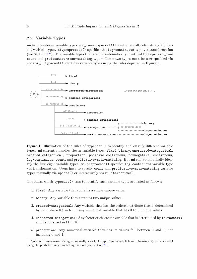
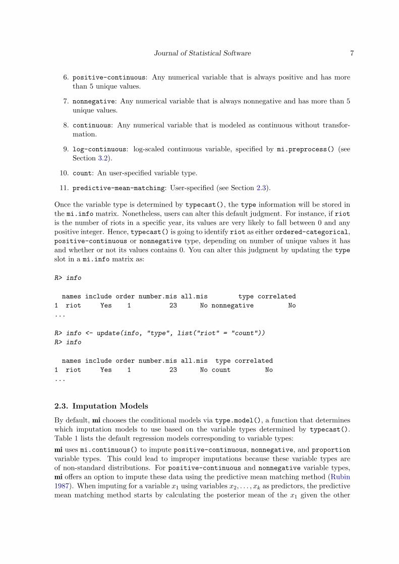
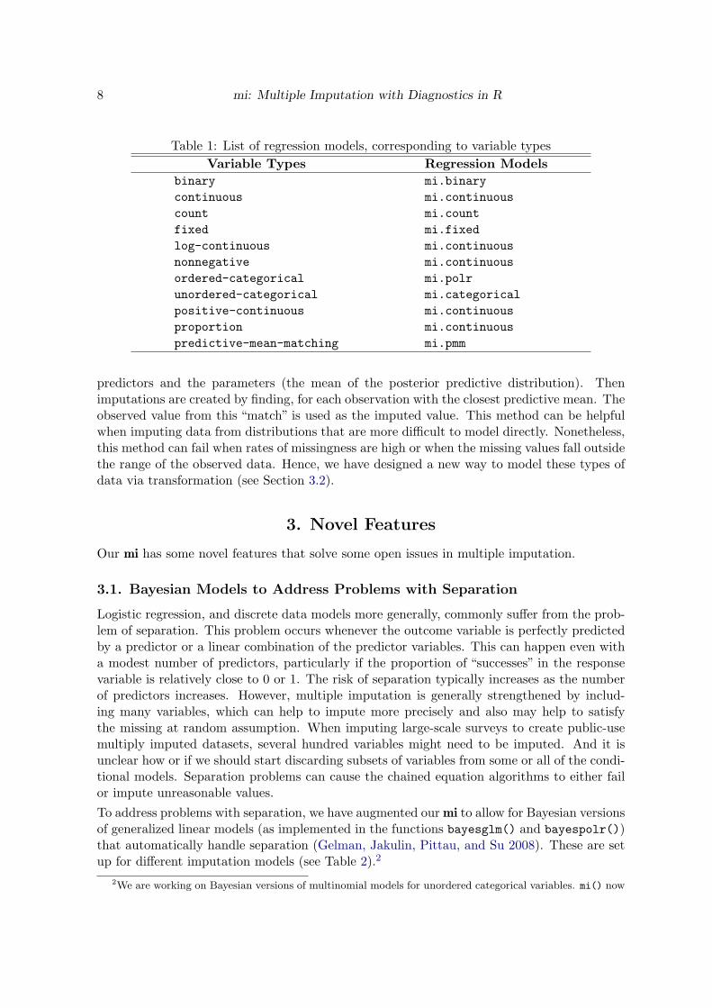
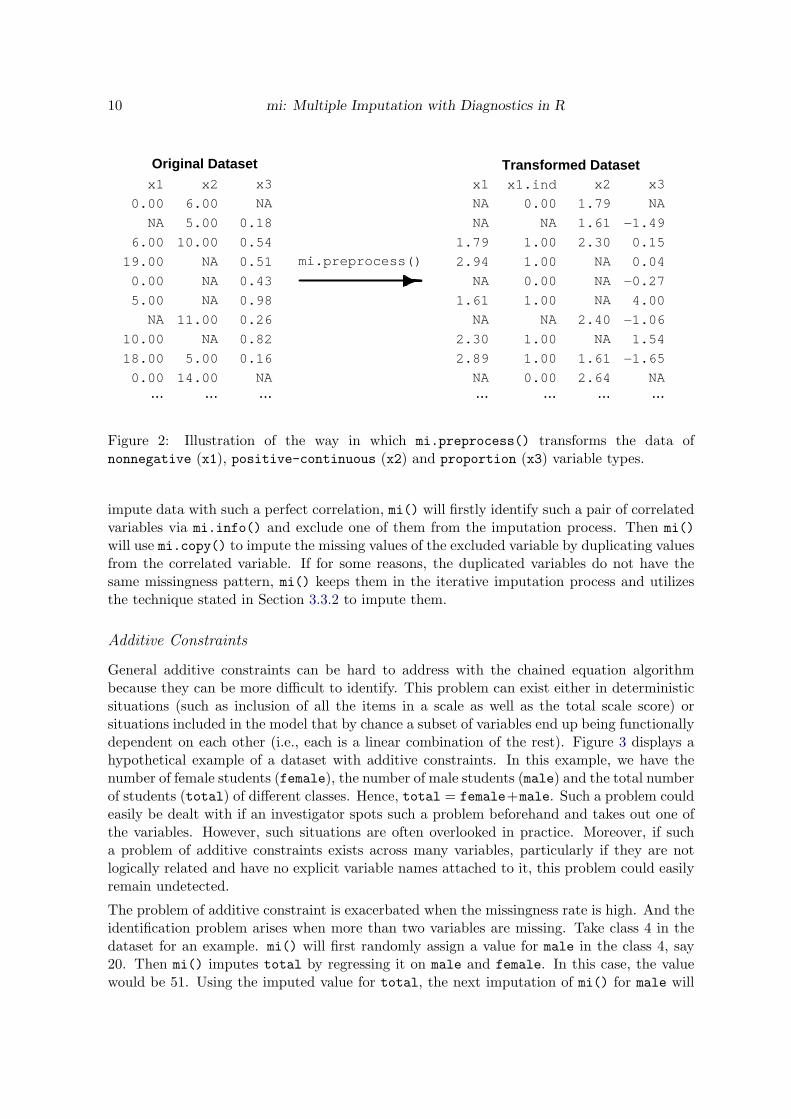
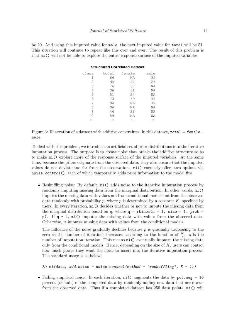
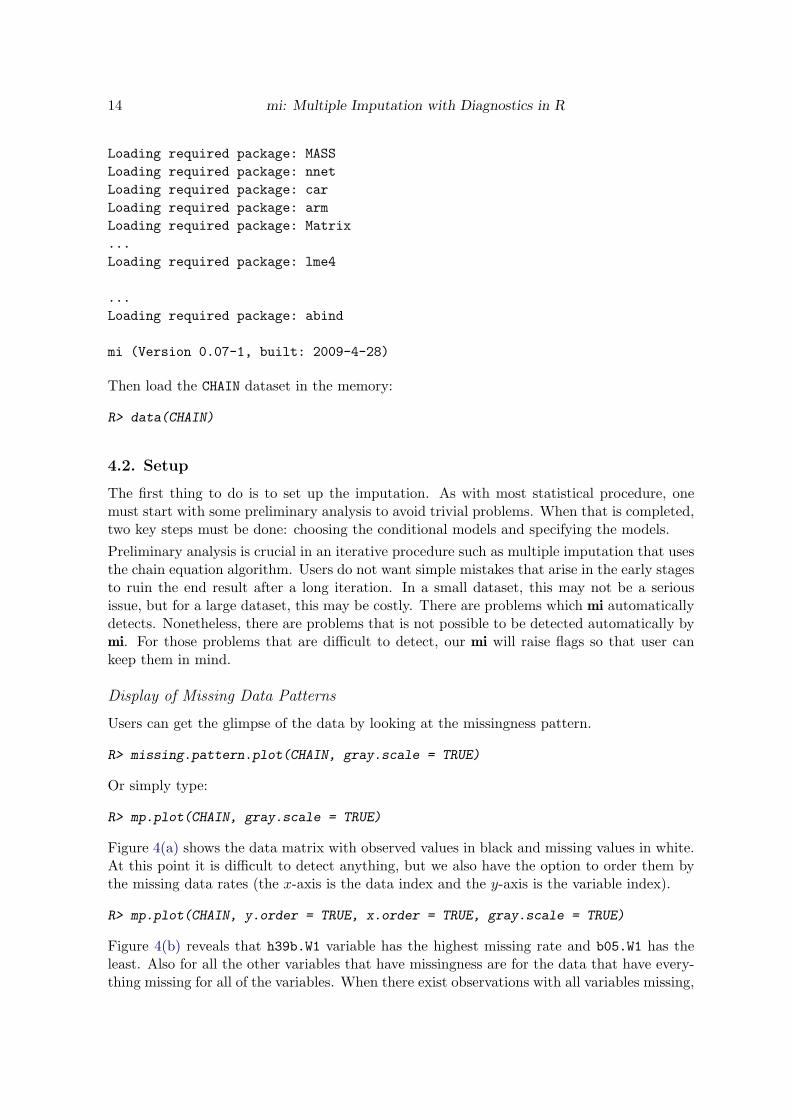
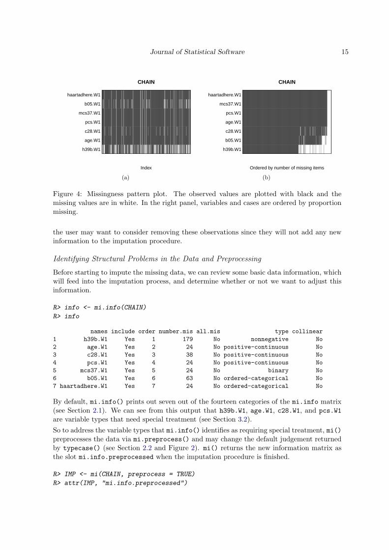


![[MI] Multiple Imputation - Duke Universitypublic.econ.duke.edu/stata/Stata-13-Documentation/mi.pdf · 2013-06-12 · Multiple imputation (MI) is a flexible, simulation-based statistical](https://static.fdocuments.net/doc/165x107/5eb947f7f1f4b4048d5334ef/mi-multiple-imputation-duke-2013-06-12-multiple-imputation-mi-is-a-iexible.jpg)


![UNDERSTANDING AND ADDRESSING MISSING DATAterm:name]/[node:create:custom:Ym... · Maximum likelihood (ML) is simpler to implement Multiple imputation (MI) can handle various types](https://static.fdocuments.net/doc/165x107/5e20cc805e07514fce330f86/understanding-and-addressing-missing-data-termnamenodecreatecustomym.jpg)


![[MI] Multiple Imputation - Stata](https://static.fdocuments.net/doc/165x107/62039c6dda24ad121e4b6a82/mi-multiple-imputation-stata.jpg)