
Multiple Criteria and Goal Programming
29
423 14 Multiple Criteria and Goal Programming 14.1 Introduction Until now, we have assumed a single objective or criterion. In reality, however, there may be two or more measures of goodness. Our life becomes more difficult, or at least more interesting, if these multiple criteria are incommensurate (i.e., it is difficult to combine them into a single criterion). The overused phrase for lamenting the difficulty of such situations is “You can’t mix apples and oranges”. Some examples of incommensurate criteria are: risk vs. return on investment, short-term profits vs. long-term growth of a firm, cost vs. service by a government agency, the treatment of different individuals un der some policy of an administrative agency (e.g., rural vs. urban citizens, residents near an airport vs. travelers using an airport, and fishermen vs. water transportation companies vs. farmers using irrigation near a large lake). Multi-criteria situations can be classified into several categories: 1. Criteria are intrinsically different (e.g., risk vs. return, cost vs. service). a) Weights or trade-off rates can be determined; b) Criteria can be strictly ordered by importance. We have so-called preemptive objectives. 2. Criteria are in trinsically similar (i.e., in some sense they should h ave equa l weight). A rich source of multi-criteria problems is the design and operation of public works. A specific example is the huge “Three Gorges” dam on the Yangtze River in China. Interested parties include: (a) industrial users of electricity, who would like the average water level in the dam to be high, so as to maximize the amount of electricity that can be generated; (b) farmers downstream from the dam, who would like the water level in the dam to be maintained at a low level, so unexpected large rainfalls can be accommodated without overflow and flooding; (c) river shipping i nterests, who would like the la ke level to be allowed to fluctuate as necessary, so as to maintain a steady flow rate out of the dam,
-
Upload
hanif-ramdhani -
Category
Documents
-
view
227 -
download
0
Transcript of Multiple Criteria and Goal Programming
7/25/2019 Multiple Criteria and Goal Programming
http://slidepdf.com/reader/full/multiple-criteria-and-goal-programming 1/29
423
14
Multiple Criteria and GoalProgramming
14.1 Introduction
Until now, we have assumed a single objective or criterion. In reality, however, there may be two ormore measures of goodness. Our life becomes more difficult, or at least more interesting, if thesemultiple criteria are incommensurate (i.e., it is difficult to combine them into a single criterion). Theoverused phrase for lamenting the difficulty of such situations is “You can’t mix apples and oranges”.
Some examples of incommensurate criteria are:
risk vs. return on investment,
short-term profits vs. long-term growth of a firm,
cost vs. service by a government agency,
the treatment of different individuals under some policy of an administrative agency(e.g., rural vs. urban citizens, residents near an airport vs. travelers using an airport, andfishermen vs. water transportation companies vs. farmers using irrigation near a largelake).
Multi-criteria situations can be classified into several categories:
1. Criteria are intrinsically different (e.g., risk vs. return, cost vs. service).a) Weights or trade-off rates can be determined;
b) Criteria can be strictly ordered by importance. We have so-called preemptiveobjectives.
2. Criteria are intrinsically similar (i.e., in some sense they should have equal weight).
A rich source of multi-criteria problems is the design and operation of public works. A specificexample is the huge “Three Gorges” dam on the Yangtze River in China. Interested parties include: (a)industrial users of electricity, who would like the average water level in the dam to be high, so as tomaximize the amount of electricity that can be generated; (b) farmers downstream from the dam, whowould like the water level in the dam to be maintained at a low level, so unexpected large rainfalls can
be accommodated without overflow and flooding; (c) river shipping interests, who would like the lakelevel to be allowed to fluctuate as necessary, so as to maintain a steady flow rate out of the dam,

7/25/2019 Multiple Criteria and Goal Programming
http://slidepdf.com/reader/full/multiple-criteria-and-goal-programming 2/29
424 Chapter 14 Multiple Criteria & Goal Programming
thereby allowing year round river travel by large ships below the dam; (d) lake fishermen andrecreational interests, who would like the flow rate out of the dam to be allowed to fluctuate asnecessary, so as to maintain a steady lake level; e) irrigation water users who would like the lake level
to be high and to be allowed to use water for irrigation than for power generation, and (f)environmental interests, who did not want the dam built in the first place. For the Three Gorges dam in particular, flood control interests have argued for having the water level behind the dam held at 459feet above sea level just before the rainy season, so as to accommodate storm runoff (see, for example,Fillon (1996)). Electricity generation interests, however, have argued for a water level of 574 feetabove sea level to generate more electricity.
14.1.1 Alternate Optima and Multicriteria
If you have a model with alternate optimal solutions, this is nature’s way of telling you that you havemultiple criteria. You should probably look at your objective function more closely and add moredetail. Users do not like alternate optima. If there are alternate optima, the typical solution method willessentially choose among them randomly. If people’s jobs or salaries depend upon the “flip of a coin”
in your analysis, they are going to be unhappy. Even if careers are not at stake, alternate optima are atleast a nuisance. People find it disconcerting if they get different answers (albeit with the sameobjective value) when they solve the same problem on different computers.
One resolution of alternate optima that might occur to some readers is to take the average of alldistinct alternate optima and use this average solution as the final, unique, well-defined answer.Unfortunately, this is usually not practical because:
a) it may be difficult to enumerate all alternate optima, and b) the average solution may be unattractive or even infeasible if the model involves integer
variables.
14.2 Approaches to Multi-criteria ProblemsThere is a variety of approaches to dealing with multiple criteria. Some of the more practical ones are
described below.
14.2.1 Pareto Optimal Solutions and Multiple CriteriaA solution to a multi-criteria problem is said to be Pareto optimal if there is no other solution that is atleast as good according to all criteria and strictly better according to at least one criterion. A Paretooptimal solution is not dominated by any other solution. Clearly, we want to consider only Paretooptimal solutions. If we do not choose our criteria carefully, we might find ourselves recommendingsolutions that are not Pareto optimal. There are computer programs for multi-criteria linear
programming that will generate all the undominated extreme solutions. For a small problem, a decisionmaker could simply choose the most attractive extreme solution based on subjective criteria. For large
problems, the number of undominated extreme solutions may easily exceed 100, so this approach may be overwhelming.
14.2.2 Utility Function ApproachA superficially attractive solution of the multi-criteria problem is the definition of a utility function. Ifthe decision variables are x1, x2, …, xn, we “simply” construct the utility function u( x1, x2, …., xn)
which computes the value or utility of any possible combination of values for the vector x1, x2, …., xn.This is a very useful approach for thinking about optimization. However, it has several practical

7/25/2019 Multiple Criteria and Goal Programming
http://slidepdf.com/reader/full/multiple-criteria-and-goal-programming 3/29
Multiple Criteria & Goal Programming Chapter 14 425
limitations: (a) it may take a lot of work to construct it, and (b) it will probably be highly nonlinear.Feature (b) means we probably cannot use LP to solve the problem.
14.2.3 Trade-off CurvesIf we have only two or three criteria, then the trade-off curve approach has most of the attractivefeatures of the utility function approach, but is also fairly practical. We simply construct a curve, theso-called “efficient frontier”, which shows how we can trade off one criterion for another. One of the
most well known settings using a trade-off curve is to describe the relationship between two criteria ina financial portfolio. The two criteria are expected return on investment and risk. We want return to behigh and risk to be low. Figure 14.1 shows the typical relationship between risk and return. Each pointon the curve is Pareto optimal. That is, for any point on the curve, there is no other point with higher
expected return and lower risk.Even though a decision maker has not gone through the trouble of constructing his utility function,he may be able to look at this trade-off curve and perhaps say: “Gee, I am comfortable with an expected return of 8% with standard deviation of 3%.”
Figure 14.1 Trade-off Curve for Risk and Expected Return
Expected
Return
Risk(e.g., Standard Deviation in Return)
0
0
14.2.4 Example: Ad Lib MarketingAd Lib is a freewheeling advertising agency that wants to solve a so-called media selection problemfor one of its clients. It is considering placing ads in five media: late night TV ( TVL), prime time TV(TVP ), billboards ( BLB), newspapers ( NEW ), and radio ( RAD). These ads are intended to reach sevendifferent demographic groups.
7/25/2019 Multiple Criteria and Goal Programming
http://slidepdf.com/reader/full/multiple-criteria-and-goal-programming 4/29
426 Chapter 14 Multiple Criteria & Goal Programming
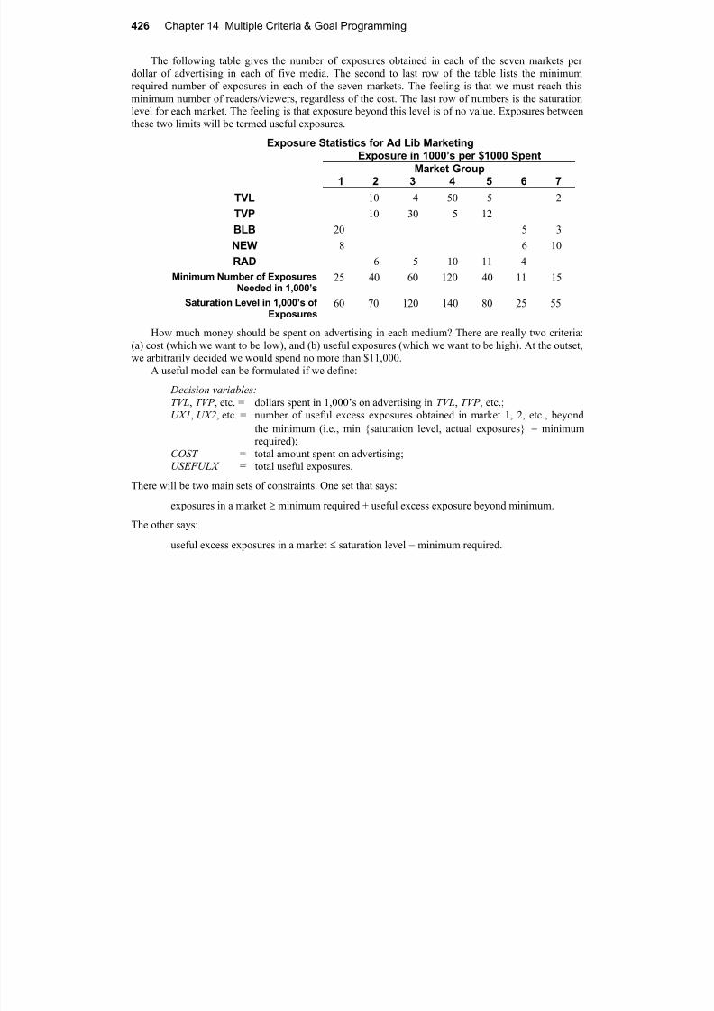
The following table gives the number of exposures obtained in each of the seven markets perdollar of advertising in each of five media. The second to last row of the table lists the minimumrequired number of exposures in each of the seven markets. The feeling is that we must reach this
minimum number of readers/viewers, regardless of the cost. The last row of numbers is the saturationlevel for each market. The feeling is that exposure beyond this level is of no value. Exposures betweenthese two limits will be termed useful exposures.
Exposure Statistics for Ad Lib MarketingExposure in 1000’s per $1000 Spent
Market Group1 2 3 4 5 6 7
TVL 10 4 50 5 2
TVP 10 30 5 12
BLB 20 5 3
NEW 8 6 10
RAD 6 5 10 11 4
Minimum Number of ExposuresNeeded in 1,000’s
25 40 60 120 40 11 15
Saturation Level in 1,000’s of
Exposures
60 70 120 140 80 25 55
How much money should be spent on advertising in each medium? There are really two criteria:(a) cost (which we want to be low), and (b) useful exposures (which we want to be high). At the outset,we arbitrarily decided we would spend no more than $11,000.
A useful model can be formulated if we define:
Decision variables:
TVL, TVP , etc. = dollars spent in 1,000’s on advertising in TVL, TVP , etc.;
UX1, UX2, etc. = number of useful excess exposures obtained in market 1, 2, etc., beyondthe minimum (i.e., min {saturation level, actual exposures} minimumrequired);
COST = total amount spent on advertising;USEFULX = total useful exposures.
There will be two main sets of constraints. One set that says:
exposures in a market minimum required + useful excess exposure beyond minimum.
The other says:
useful excess exposures in a market saturation level minimum required.
7/25/2019 Multiple Criteria and Goal Programming
http://slidepdf.com/reader/full/multiple-criteria-and-goal-programming 5/29
Multiple Criteria & Goal Programming Chapter 14 427
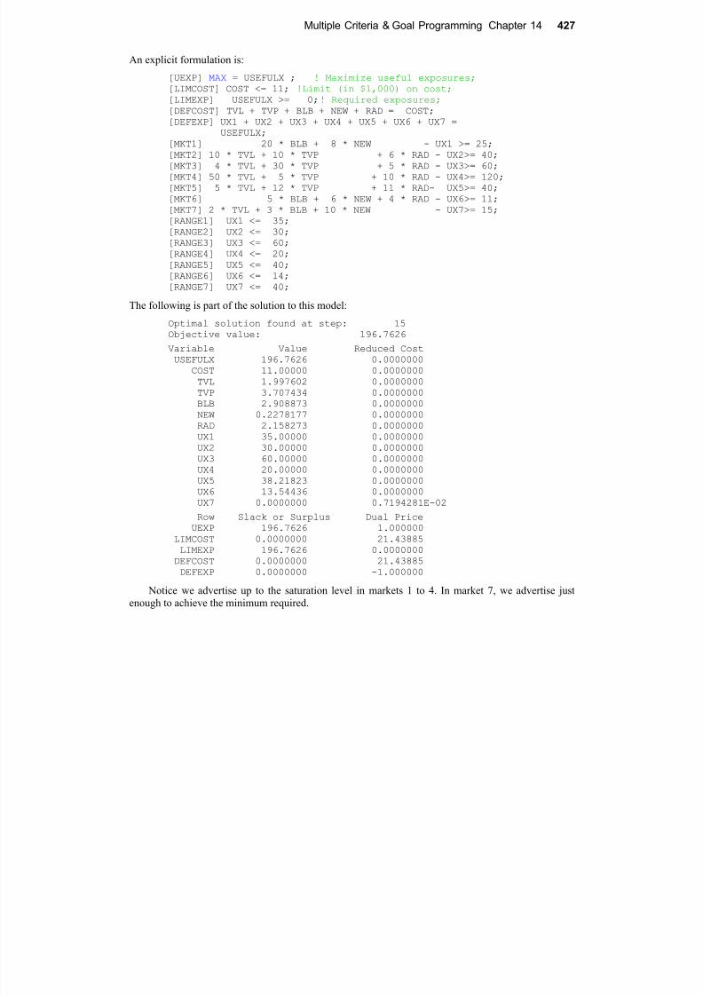
An explicit formulation is:
[UEXP] MAX = USEFULX ; ! Maximize useful exposures;
[LIMCOST] COST <= 11; !Limit (in $1,000) on cost;
[LIMEXP] USEFULX >= 0;! Required exposures; [DEFCOST] TVL + TVP + BLB + NEW + RAD = COST;
[DEFEXP] UX1 + UX2 + UX3 + UX4 + UX5 + UX6 + UX7 =
USEFULX;
[MKT1] 20 * BLB + 8 * NEW - UX1 >= 25;
[MKT2] 10 * TVL + 10 * TVP + 6 * RAD - UX2>= 40;
[MKT3] 4 * TVL + 30 * TVP + 5 * RAD - UX3>= 60;
[MKT4] 50 * TVL + 5 * TVP + 10 * RAD - UX4>= 120;
[MKT5] 5 * TVL + 12 * TVP + 11 * RAD- UX5>= 40;
[MKT6] 5 * BLB + 6 * NEW + 4 * RAD - UX6>= 11;
[MKT7] 2 * TVL + 3 * BLB + 10 * NEW - UX7>= 15;
[RANGE1] UX1 <= 35;
[RANGE2] UX2 <= 30;
[RANGE3] UX3 <= 60;
[RANGE4] UX4 <= 20;
[RANGE5] UX5 <= 40;
[RANGE6] UX6 <= 14;
[RANGE7] UX7 <= 40;
The following is part of the solution to this model:Optimal solution found at step: 15
Objective value: 196.7626
Variable Value Reduced Cost
USEFULX 196.7626 0.0000000
COST 11.00000 0.0000000
TVL 1.997602 0.0000000
TVP 3.707434 0.0000000
BLB 2.908873 0.0000000
NEW 0.2278177 0.0000000
RAD 2.158273 0.0000000
UX1 35.00000 0.0000000
UX2 30.00000 0.0000000
UX3 60.00000 0.0000000
UX4 20.00000 0.0000000
UX5 38.21823 0.0000000
UX6 13.54436 0.0000000
UX7 0.0000000 0.7194281E-02
Row Slack or Surplus Dual Price
UEXP 196.7626 1.000000
LIMCOST 0.0000000 21.43885
LIMEXP 196.7626 0.0000000
DEFCOST 0.0000000 21.43885
DEFEXP 0.0000000 -1.000000
Notice we advertise up to the saturation level in markets 1 to 4. In market 7, we advertise justenough to achieve the minimum required.

7/25/2019 Multiple Criteria and Goal Programming
http://slidepdf.com/reader/full/multiple-criteria-and-goal-programming 6/29
428 Chapter 14 Multiple Criteria & Goal Programming
If you change the cost limit (initially at 11) to various values ranging from 6 to 14 and plot themaximum possible number of useful exposures, you get a trade-off curve, or efficient frontier, shownin the Figure 14.2:
Figure 14.2 Trade-off Between Exposures and Advertising
Useful
Excess
Exposures
Advertising Expenditure
6 7 8 9 10 11 12 13 14
30
60
90
120
150
180
210
240
14.3 Goal Programming and Soft ConstraintsGoal Programming is closely related to the concept of multi-criteria as well as a simple idea that wedub “soft constraints”. Soft constraints and Goal Programming are a response to the following two
“laws of the real world”.
In the real world:
1) there is always a feasible solution;2) there are no alternate optima.
In practical terms, (1) means a good manager (or one wishing to at least keep a job) never throwsup his or her hands in despair and says “no feasible solution”. Law (2) means a typical decision maker
will never be indifferent between two proposed courses of action. There are always sufficient criteriato distinguish some course of action as better than all others.
From a model perspective, these two laws mean a well-formulated model (a) always has a feasiblesolution and (b) does not have alternate optima.

7/25/2019 Multiple Criteria and Goal Programming
http://slidepdf.com/reader/full/multiple-criteria-and-goal-programming 7/29
Multiple Criteria & Goal Programming Chapter 14 429
14.3.1 Example: Secondary Criterion to Choose Among Alternate OptimaHere is a standard, seven-day/week staffing problem similar to that discussed in Chapter 7. Thevariables: M , T , W , R, F , S , N , denote the number of people starting their five-day work week on
Monday, Tuesday, Wednesday, Thursday, Friday, Saturday, or Sunday, respectively:MIN = 9*M + 9*T + 9*W + 9*R + 9*F + 9*S + 9*N;
[MON] M + R + F + S + N 3;
[TUE] M + T + F + S + N 3;
[WED] M + T + W + S + N 8;
[THU] M + T + W + R + N 8;
[FRI] M + T + W + R + F 8;
[SAT] T + W + R + F + S 3;
[SUN] W + R + F + S + N 3;END
When solved, we get the following solution:
Optimal solution found at step: 6
Objective value: 72.00000
Variable Value Reduced Cost
M 5.000000 0.0000000
T 0.0000000 0.0000000
W 3.000000 0.0000000
R 0.0000000 0.0000000
F 0.0000000 9.000000
S 0.0000000 9.000000
N 0.0000000 0.0000000
Row Slack or Surplus Dual Price
1 72.00000 1.000000
MON 2.000000 0.0000000
TUE 2.000000 0.0000000
WED 0.0000000 0.0000000
THU 0.0000000 -9.000000
FRI 0.0000000 0.0000000
SAT 0.0000000 0.0000000
SUN 0.0000000 0.0000000
Notice there may be alternate optima (e.g., the slack and dual price in row “WED” are both zero).
This solution puts all the surplus capacity on Saturday and Sunday. The different optima mightdistribute the surplus capacity in different ways over the days of the week. Saturday and Sunday have a
lot of excess capacity while the very similar days, Monday and Tuesday, have no surplus capacity.In terms of multiple criteria, we might say:
a) our most important criterion is to minimize total staffing cost; b) our secondary criterion is to have a little extra capacity, specifically one unit, each day if
it will not hurt criterion 1.

7/25/2019 Multiple Criteria and Goal Programming
http://slidepdf.com/reader/full/multiple-criteria-and-goal-programming 8/29
430 Chapter 14 Multiple Criteria & Goal Programming
To encourage more equitable distribution, we add some “excess” variables ( XM , XT , etc.) that
give a tiny credit of 1 for each surplus up to at most 1 on each day. The modified formulation is:
MODEL:
MIN = 9*M + 9*T + 9*W + 9*R + 9*F + 9*S + 9*N- XM - XT - XW - XR - XF - XS - XN;
[MON] M + R + F + S + N - XM 3;
[TUE] M + T + F + S + N - XT 3;
[WED] M + T + W + S + N - XW 8;
[THU] M + T + W + R + N - XR 8;
[FRI] M + T + W + R + F - XF 8;
[SAT] T + W + R + F + S - XS 3;
[SUN] W + R + F + S + N - XN 3;
[N9] XM 1;
[N10] XT 1;
[N11] XW 1;
[N12] XR 1;
[N13] XF 1;
[N14] XS 1;
[N15] XN 1;
END
The solution now is:
Optimal solution found at step: 19
Objective value: 68.00000
Variable Value Reduced Cost
M 4.000000 0.0000000
T 0.0000000 0.0000000
W 4.000000 0.0000000
R 0.0000000 1.000000F 0.0000000 8.000000
S 0.0000000 8.000000
N 0.0000000 1.000000
XM 1.000000 0.0000000
XT 1.000000 0.0000000
XW 0.0000000 0.0000000
XR 0.0000000 6.000000
XF 0.0000000 0.0000000
XS 1.000000 0.0000000
XN 1.000000 0.0000000
Notice, just as before, we still hire a total of eight people, but now the surplus is evenly distributedover the four days M , T , S , and N . This should be a more attractive solution.

7/25/2019 Multiple Criteria and Goal Programming
http://slidepdf.com/reader/full/multiple-criteria-and-goal-programming 9/29
Multiple Criteria & Goal Programming Chapter 14 431
14.3.2 Preemptive/Lexico Goal ProgrammingThe above approach required us to choose the proper relative weights for our two objectives, cost andservice. In some situations, it may be clear that one objective is orders of magnitude more important
than the other. One could choose weights to reflect this (e.g., 99999999 for the first and 0.0000001 forthe second), but there are a variety of reasons for not using this approach. First of all, there would probably be numerical problems, especially if there are more than two objectives. A typical computercannot accurately add numbers that differ by more than 15 orders of magnitude (e.g., 100,000,000 and.0000001).
More importantly, it just seems more straightforward simply to say: “This first objective is far
more important than the remaining objectives, the second objective is far more important than theremaining objectives,” etc. This approach is sometimes called Preemptive or Lexico goal
programming. The following illustrates for our previous staff-scheduling example. The first modelsolved places a weight of 1.0 on the more important objective, COST , and no weight on the secondaryobjective, EXTRA credit for useful overstaffing:
!Example of Lexico-goal programming
MIN = 1 * COST - 0 * EXTRA;
[MON] M + R + F + S + N - XM >= 3;
[TUE] M + T + F + S + N - XT >= 3;
[WED] M + T + W + S + N - XW >= 8;
[THU] M + T + W + R + N - XR >= 8;
[FRI] M + T + W + R + F - XF >= 8;[SAT] T + W + R + F + S - XS >= 3;
[SUN] W + R + F + S + N - XN >= 3;
! Upper limit on creditable excess;
[EXM] XM <= 1;
[EXT] XT <= 1;
[EXW] XW <= 1;
[EXR] XR <= 1;
[EXF] XF <= 1;
[EXS] XS <= 1;[EXN] XN <= 1;
! Define the two objectives;
[OBJCOST] COST = M + R + F + S + N + T + W;
[OBJXTRA] EXTRA = XM + XT + XW + XR + XF + XS + XN;
END
7/25/2019 Multiple Criteria and Goal Programming
http://slidepdf.com/reader/full/multiple-criteria-and-goal-programming 10/29
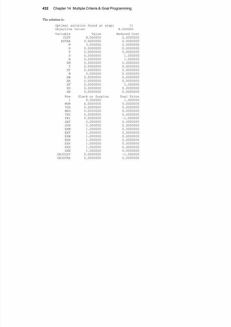
432 Chapter 14 Multiple Criteria & Goal Programming
The solution is:
Optimal solution found at step: 11
Objective value: 8.000000
Variable Value Reduced CostCOST 8.000000 0.0000000
EXTRA 0.0000000 0.0000000
M 3.000000 0.0000000
R 0.0000000 0.0000000
F 0.0000000 0.0000000
S 0.0000000 1.000000
N 0.0000000 1.000000
XM 0.0000000 0.0000000
T 0.0000000 0.0000000XT 0.0000000 0.0000000
W 5.000000 0.0000000
XW 0.0000000 0.0000000
XR 0.0000000 0.0000000
XF 0.0000000 1.000000
XS 0.0000000 0.0000000
XN 0.0000000 0.0000000
Row Slack or Surplus Dual Price
1 8.000000 1.000000
MON 0.0000000 0.0000000
TUE 0.0000000 0.0000000
WED 0.0000000 0.0000000
THU 0.0000000 0.0000000
FRI 0.0000000 -1.000000
SAT 2.000000 0.0000000
SUN 2.000000 0.0000000
EXM 1.000000 0.0000000
EXT 1.000000 0.0000000
EXW 1.000000 0.0000000EXR 1.000000 0.0000000
EXF 1.000000 0.0000000
EXS 1.000000 0.0000000
EXN 1.000000 0.0000000
OBJCOST 0.0000000 -1.000000
OBJXTRA 0.0000000 0.0000000
7/25/2019 Multiple Criteria and Goal Programming
http://slidepdf.com/reader/full/multiple-criteria-and-goal-programming 11/29
Multiple Criteria & Goal Programming Chapter 14 433
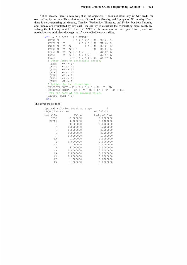
Notice because there is zero weight in the objective, it does not claim any EXTRA credit foroverstaffing by one unit. This solution starts 3 people on Monday, and 5 people on Wednesday. Thus,there is no overstaffing on Monday, Tuesday, Wednesday, Thursday, and Friday, but both Saturdayand Sunday are overstaffed by two each. We can try to distribute the overstaffing more evenly bysolving the following model. It fixes the COST at the minimum we have just learned, and nowmaximizes (or minimizes the negative of) the creditable extra staffing:
MIN = 0 * COST - 1 * EXTRA;
[MON] M + R + F + S + N - XM >= 3;
[TUE] M + T + F + S + N - XT >= 3;
[WED] M + T + W + S + N - XW >= 8;
[THU] M + T + W + R + N - XR >= 8;
[FRI] M + T + W + R + F - XF >= 8;
[SAT] T + W + R + F + S - XS >= 3;[SUN] W + R + F + S + N - XN >= 3;
! Upper limit on creditable excess;
[EXM] XM <= 1;
[EXT] XT <= 1;
[EXW] XW <= 1;
[EXR] XR <= 1;
[EXF] XF <= 1;
[EXS] XS <= 1;
[EXN] XN <= 1;! Define the two objectives;
[OBJCOST] COST = M + R + F + S + N + T + W;
[OBJXTRA] EXTRA = XM + XT + XW + XR + XF + XS + XN;
! Fix the cost at its minimum value;
[FXCOST] COST = 8;
END
This gives the solution:
Optimal solution found at step: 7Objective value: -4.000000
Variable Value Reduced Cost
COST 8.000000 0.0000000
EXTRA 4.000000 0.0000000
M 4.000000 0.0000000
R 0.0000000 1.000000
F 0.0000000 2.000000
S 0.0000000 2.000000
N 0.0000000 1.000000XM 1.000000 0.0000000
T 0.0000000 0.0000000
XT 1.000000 0.0000000
W 4.000000 0.0000000
XW 0.0000000 0.0000000
XR 0.0000000 0.0000000
XF 0.0000000 0.0000000
XS 1.000000 0.0000000
XN 1.000000 0.0000000
7/25/2019 Multiple Criteria and Goal Programming
http://slidepdf.com/reader/full/multiple-criteria-and-goal-programming 12/29
434 Chapter 14 Multiple Criteria & Goal Programming
Row Slack or Surplus Dual Price
1 -4.000000 -1.000000
MON 0.0000000 0.0000000
TUE 0.0000000 0.0000000
WED 0.0000000 -1.000000THU 0.0000000 -1.000000
FRI 0.0000000 -1.000000
SAT 0.0000000 0.0000000
SUN 0.0000000 0.0000000
EXM 0.0000000 1.000000
EXT 0.0000000 1.000000
EXW 1.000000 0.0000000
EXR 1.000000 0.0000000
EXF 1.000000 0.0000000
EXS 0.0000000 1.000000
EXN 0.0000000 1.000000
OBJCOST 0.0000000 -3.000000
OBJXTRA 0.0000000 1.000000
FXCOST 0.0000000 3.000000
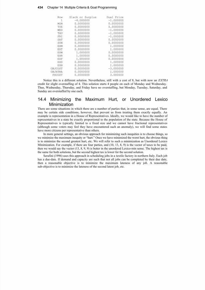
Notice this is a different solution. Nevertheless, still with a cost of 8, but with now an EXTRA credit for slight overstaffing of 4. This solution starts 4 people on each of Monday and Wednesday.Thus, Wednesday, Thursday, and Friday have no overstaffing, but Monday, Tuesday, Saturday, and
Sunday are overstaffed by one each.
14.4 Minimizing the Maximum Hurt, or Unordered LexicoMinimization
There are some situations in which there are a number of parties that, in some sense, are equal. Theremay be certain side conditions, however, that prevent us from treating them exactly equally. Anexample is representation in a House of Representatives. Ideally, we would like to have the number of
representatives in a state be exactly proportional to the population of the state. Because the House ofRepresentatives is typically limited to a fixed size and we cannot have fractional representatives(although some voters may feel they have encountered such an anomaly), we will find some stateshave more citizens per representative than others.
In more general settings, an obvious approach for minimizing such inequities is to choose things, sowe minimize the maximum inequity or “hurt.” Once we have minimized the worst hurt, the obvious thing
is to minimize the second greatest hurt, etc. We will refer to such a minimization as Unordered LexicoMinimization. For example, if there are four parties, and (10, 13, 8, 9) is the vector of taxes to be paid,
then we would say the vector (13, 8, 9, 9) is better in the unordered Lexico-min sense. The highest tax isthe same for both solutions, but the second highest tax is lower for the second solution.Serafini (1996) uses this approach in scheduling jobs in a textile factory in northern Italy. Each job
has a due-date. If demand and capacity are such that not all jobs can be completed by their due date,then a reasonable objective is to minimize the maximum lateness of any job. A reasonablesub-objective is to minimize the lateness of the second latest job, etc.

7/25/2019 Multiple Criteria and Goal Programming
http://slidepdf.com/reader/full/multiple-criteria-and-goal-programming 13/29
Multiple Criteria & Goal Programming Chapter 14 435
14.4.1 ExampleThis example is based on one in Sankaran (1989). There are six parties and xi is the assessment to be
paid by party i to satisfy a certain community building project. The xi must satisfy the set of
constraints:A. X1 + 2 X2 + 4 X3 + 7 X4 16
B. 2.5 X1 + 3.5 X2 + 5.2 X5 17.5
C. 0.4 X2 + 1.3 X4 + 7.2 X6 12
D. 2.5 X2 + 3.5 X3 + 5.2 X5 13.1
E. 3.5 X1 + 3.5 X4 + 5.2 X6 18.2
We would like to minimize the highest assessment paid by anyone. Given that, we would like to
minimize the second highest assessment paid by anyone. Given that, we would like to minimize thethird highest, etc. The interested reader may try to improve upon the following set of assessments:
X1 = 1.5625 X2 = 1.5625 X3 = .305357 X4 = 1.463362 X5 = 1.5625 X6 = 1.463362
There is no other solution in which:
a) the highest assessment is less than 1.5625, and b) the second highest assessment is less than 1.5625, andc) the third highest assessment is less than 1.5625, andd) the fourth highest assessment is less than 1.463362, etc.
14.4.2 Finding a Unique Solution Minimizing the Maximum
A quite general approach to finding a unique unordered Lexico minimum exists when the feasibleregion is convex (i.e. any solution that is a positively weighted average of two feasible solutions is alsofeasible). Thus, problems with integer variables are not convex. Let the vector { x1, x2, …, xn} denotethe cost allocated to each of n parties.
If the feasible region is convex, then there is a unique solution and the following algorithm willfind it. Maschler, Peleg, and Shapley (1979) discuss this idea in the game theory setting, where the“nucleolus” is a closely related concept. If the feasible region is not convex (e.g., the problem hasinteger variables), then the following method is not guaranteed to find the solution. Let S be the
original set of constraints on the x’s.
1) Let J = {1, 2, . . . , n}, and k = 0; (Note: J is the set of parties for whom we do not yetknow the final xi)
2) Let k = k + 1;

7/25/2019 Multiple Criteria and Goal Programming
http://slidepdf.com/reader/full/multiple-criteria-and-goal-programming 14/29
436 Chapter 14 Multiple Criteria & Goal Programming
3) Solve the problem:Minimize Z subject to
x feasible to S and, Z > x j for j in J (Note: this finds the minimum, maximum hurt among parties for which we have notyet fixed the x j’s.);
4) Set Z k = Z of (3), and add to S the constraints: x j < Z k for all j in J ;
5) Set L = { j in J for which x j = Z k in (3)}:For each j in L:
Solve:
Minimize x j subject to
x feasible to S ;
If x j = Z k , then set J = J j, and append to S the constraint x j = Z k 6) If J is not empty, go to (2), else we are done.
To find the minimum maximum assessment for our example problem, we solve the following problem:
MODEL:MIN = Z;
! The physical constraints on the X's;
[A] X1 + 2*X2 + 4*X3 + 7*X4 >= 16;
[B] 2.5*X1 + 3.5*X2 + 5.2*X5 >= 17.5;
[C] 0.4*X2 + 1.3*X4 + 7.2*X6 >= 12;
[D] 2.5*X2 + 3.5*X3 + 5.2*X5 >= 13.1;
[E] 3.5*X1 + 3.5*X4 + 5.2*X6 >= 18.2;
! Constraints to compute the max hurt Z;
[H1] Z - X1 >= 0;
[H2] Z - X2 >= 0;
[H3] Z - X3 >= 0;
[H4] Z - X4 >= 0;
[H5] Z - X5 >= 0;
[H6] Z - X6 >= 0;
END
Its solution is:
Objective value: 1.5625000
Variable Value Reduced Cost
Z 1.5625000 0.0000000
X1 1.5625000 0.0000000
X2 1.5625000 0.0000000
X3 1.5625000 0.0000000
X4 1.5625000 0.0000000
X5 1.5625000 0.0000000
X6 1.5625000 0.0000000
Thus, at least one party will have a “hurt” of 1.5625. Which party or parties will it be?
M lti l C it i & G l P i Ch t 14 437

7/25/2019 Multiple Criteria and Goal Programming
http://slidepdf.com/reader/full/multiple-criteria-and-goal-programming 15/29
Multiple Criteria & Goal Programming Chapter 14 437
Because all six xi’s equal 1.5625, we solve a series of six problems such as the following:
MODEL:
MIN = X1;
! The physical constraints on the X's;
[A] X1 + 2*X2 + 4*X3 + 7*X4 >= 16;
[B] 2.5*X1 + 3.5*X2 + 5.2*X5 >= 17.5;
[C] 0.4*X2 + 1.3*X4 + 7.2*X6 >= 12;
[D] 2.5*X2 + 3.5*X3 + 5.2*X5 >= 13.1;
[E] 3.5*X1 + 3.5*X4 + 5.2*X6 >= 18.2;
! Constraints for finding the minmax hurt, Z;
[H1] X1 <= 1.5625000;
[H2] X2 <= 1.5625000;
[H3] X3 <= 1.5625000;
[H4] X4 <= 1.5625000;[H5] X5 <= 1.5625000;
[H6] X6 <= 1.5625000;
END
The solution for the case of X1 is:
Objective value: 1.5625000
Variable Value Reduced Cost
X1 1.5625000 0.0000000
X2 1.5625000 0.0000000
X3 0.3053573 0.0000000
X4 1.5625000 0.0000000
X5 1.5625000 0.0000000
X6 1.3966350 0.0000000
Thus, there is no solution with all the xi’s < 1.5625, but with X1 strictly less than 1.5625. So, wecan fix X1 at 1.5625. Similar observations turn out to be true for X2 and X5.
So, now we wish to solve the following problem:
MODEL:
MIN = Z;
! The physical constraints on the X's;
X1 + 2*X2 + 4*X3 + 7*X4 >= 16;
2.5*X1 + 3.5*X2 + 5.2*X5 >= 17.5;
0.4*X2 + 1.3*X4 + 7.2*X6 >= 12;
2.5*X2 + 3.5*X3 + 5.2*X5 >= 13.1;
3.5*X1 + 3.5*X4 + 5.2*X6 >= 18.2;
! Constraints for finding the minmax hurt, Z;
X1 = 1.5625000;
X2 = 1.5625000;
- Z + X3 <= 0;
- Z + X4 <= 0;
X5 = 1.5625000;
- Z + X6 <= 0;
END
438 Chapter 14 Multiple Criteria & Goal Programming

7/25/2019 Multiple Criteria and Goal Programming
http://slidepdf.com/reader/full/multiple-criteria-and-goal-programming 16/29
438 Chapter 14 Multiple Criteria & Goal Programming
Upon solution, we see the second highest “hurt” is 1.4633621:
Objective value: 1.4633621
Variable Value Reduced Cost
Z 1.4633621 0.0000000X1 1.5625000 0.0000000
X2 1.5625000 0.0000000
X3 1.4633621 0.0000000
X4 1.4633621 0.0000000
X5 1.5625000 0.0000000
X6 1.4633621 0.0000000
Any or all of X3, X4 or X6 could be at this value in the final solution. Which ones? To find out, wesolve the following kind of problem for X3, X4 and X6 :
MODEL:
MIN = X3;
! The physical constraints on the X's;
[A] X1 + 2*X2 + 4*X3 + 7*X4 >= 16;
[B] 2.5*X1 + 3.5*X2 + 5.2*X5 >= 17.5;
[C] 0.4*X2 + 1.3*X4 + 7.2*X6 >= 12;
[D] 2.5*X2 + 3.5*X3 + 5.2*X5 >= 13.1;
[E] 3.5*X1 + 3.5*X4 + 5.2*X6 >= 18.2;
! Constraints for finding the minmax hurt, Z;
[H1] X1 = 1.5625000;
[H2] X2 = 1.5625000;
[H3] X3 <= 1.4633621;
[H4] X4 <= 1.4633621;
[H5] X5 = 1.5625000;
[H6] X6 <= 1.4633621;
END
The solution, when we minimize X3, is:
Objective value: .3053571400
Variable Value Reduced Cost
X3 .30535714 0.0000000
X1 1.5625000 0.0000000
X2 1.5625000 0.0000000
X4 1.4633621 0.0000000
X5 1.5625000 0.0000000
X6 1.4633621 0.0000000
Thus, X3 need not be as high as 1.4633621 in the final solution. We do find, however, that X4 and X6 can be no smaller than 1.4633621.
Multiple Criteria & Goal Programming Chapter 14 439
7/25/2019 Multiple Criteria and Goal Programming
http://slidepdf.com/reader/full/multiple-criteria-and-goal-programming 17/29
Multiple Criteria & Goal Programming Chapter 14 439
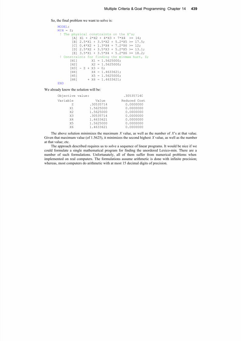
So, the final problem we want to solve is:
MODEL:
MIN = Z;
! The physical constraints on the X's;
[A] X1 + 2*X2 + 4*X3 + 7*X4 >= 16;
[B] 2.5*X1 + 3.5*X2 + 5.2*X5 >= 17.5;
[C] 0.4*X2 + 1.3*X4 + 7.2*X6 >= 12;
[D] 2.5*X2 + 3.5*X3 + 5.2*X5 >= 13.1;
[E] 3.5*X1 + 3.5*X4 + 5.2*X6 >= 18.2;
! Constraints for finding the minmax hurt, Z;
[H1] X1 = 1.5625000;
[H2] X2 = 1.5625000;
[H3] - Z + X3 = 0;
[H4] X4 = 1.4633621;[H5] X5 = 1.5625000;
[H6] + X6 = 1.4633621;
END
We already know the solution will be:
Objective value: .305357140
Variable Value Reduced Cost
Z .30535714 0.0000000
X1 1.5625000 0.0000000
X2 1.5625000 0.0000000
X3 .30535714 0.0000000
X4 1.4633621 0.0000000
X5 1.5625000 0.0000000
X6 1.4633621 0.0000000
The above solution minimizes the maximum X value, as well as the number of X ’s at that value.
Given that maximum value (of 1.5625), it minimizes the second highest X value, as well as the number
at that value; etc.The approach described requires us to solve a sequence of linear programs. It would be nice if we
could formulate a single mathematical program for finding the unordered Lexico-min. There are anumber of such formulations. Unfortunately, all of them suffer from numerical problems whenimplemented on real computers. The formulations assume arithmetic is done with infinite precision;whereas, most computers do arithmetic with at most 15 decimal digits of precision.
440 Chapter 14 Multiple Criteria & Goal Programming
7/25/2019 Multiple Criteria and Goal Programming
http://slidepdf.com/reader/full/multiple-criteria-and-goal-programming 18/29
440 Chapter 14 Multiple Criteria & Goal Programming
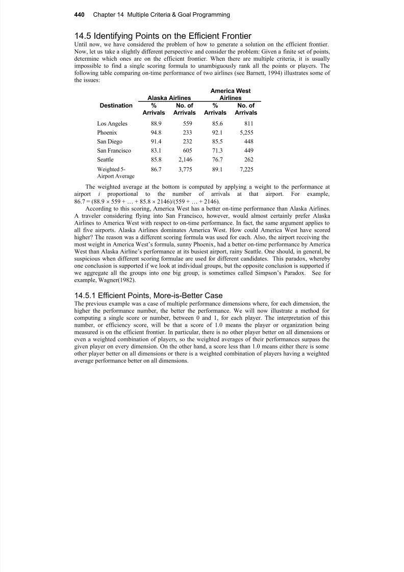
14.5 Identifying Points on the Efficient FrontierUntil now, we have considered the problem of how to generate a solution on the efficient frontier.
Now, let us take a slightly different perspective and consider the problem: Given a finite set of points,
determine which ones are on the efficient frontier. When there are multiple criteria, it is usuallyimpossible to find a single scoring formula to unambiguously rank all the points or players. Thefollowing table comparing on-time performance of two airlines (see Barnett, 1994) illustrates some ofthe issues:
Alaska AirlinesAmerica West
AirlinesDestination %
ArrivalsNo. of
Arrivals%
ArrivalsNo. of
Arrivals
Los Angeles 88.9 559 85.6 811
Phoenix 94.8 233 92.1 5,255
San Diego 91.4 232 85.5 448
San Francisco 83.1 605 71.3 449
Seattle 85.8 2,146 76.7 262
Weighted 5-
Airport Average
86.7 3,775 89.1 7,225
The weighted average at the bottom is computed by applying a weight to the performance atairport i proportional to the number of arrivals at that airport. For example,
86.7 = (88.9 559 + … + 85.8 2146)/(559 + … + 2146).According to this scoring, America West has a better on-time performance than Alaska Airlines.
A traveler considering flying into San Francisco, however, would almost certainly prefer AlaskaAirlines to America West with respect to on-time performance. In fact, the same argument applies toall five airports. Alaska Airlines dominates America West. How could America West have scored
higher? The reason was a different scoring formula was used for each. Also, the airport receiving themost weight in America West’s formula, sunny Phoenix, had a better on-time performance by AmericaWest than Alaska Airline’s performance at its busiest airport, rainy Seattle. One should, in general, besuspicious when different scoring formulae are used for different candidates. This paradox, wherebyone conclusion is supported if we look at individual groups, but the opposite conclusion is supported ifwe aggregate all the groups into one big group, is sometimes called Simpson’s Paradox. See forexample, Wagner(1982).
14.5.1 Efficient Points, More-is-Better CaseThe previous example was a case of multiple performance dimensions where, for each dimension, thehigher the performance number, the better the performance. We will now illustrate a method forcomputing a single score or number, between 0 and 1, for each player. The interpretation of thisnumber, or efficiency score, will be that a score of 1.0 means the player or organization beingmeasured is on the efficient frontier. In particular, there is no other player better on all dimensions oreven a weighted combination of players, so the weighted averages of their performances surpass thegiven player on every dimension. On the other hand, a score less than 1.0 means either there is some
other player better on all dimensions or there is a weighted combination of players having a weightedaverage performance better on all dimensions.
Multiple Criteria & Goal Programming Chapter 14 441

7/25/2019 Multiple Criteria and Goal Programming
http://slidepdf.com/reader/full/multiple-criteria-and-goal-programming 19/29
p g g p
Define:
r ij = the performance (or reward) of player i on the jth dimension (e.g., the on-time
performance of Alaska Airlines in Seattle);
v j = the weight or value to be applied to the jth
dimension in evaluating overall efficiency.To evaluate the performance of player k, we will do the following in words:
Choose the v j so as to maximize score (k )subject to
For each player i (including k ):
score (i) 1.
More precisely, we want to:
Max j v j r kj subject to
For every player i, including k :
j v j r ij 1For every weight j:
v j e,
where e is a small positive number.The reason for requiring every v j to be slightly positive is as follows. Suppose player k and someother player t are tied for best on one dimension, say j, but player k is worse than t on all otherdimensions. Player k would like to place all the weight on dimension j, so player k will appear to be
just as efficient as player t . Requiring a small positive weight on every dimension will reveal theseslightly dominated players. Some care should be taken in the choice of the small “infinitesimal”
constant e. If it is chosen too large, it may cause the problem to be infeasible. If it is chosen too small,it may be effectively disregarded by the optimization algorithm. From the above, you can observe thatit should be bounded by:
e 1/ j r ij.
See Mehrabian, Jahanshahloo, Alirezaee, and Amin(2000) for a more detailed discussion.
Example
The performance of five high schools in the “three R’s” of “Reading, Writing and Arithmetic” are
tabulated below (see Chicago Magazine, February 1995):
School Reading Writing MathematicsBarrington 296 27 306
Lisle 286 27.1 322
Palatine 290 28.5 303
Hersey 298 27.3 312
Oak Park River Forest (OPRF) 294 28.1 301
Hersey, Palatine, and Lisle are clearly on the efficient frontier because they have the highestscores in reading, writing, and mathematics, respectively. Barrington is clearly not on the efficientfrontier, because it is dominated by Hersey. What can we say about OPRF?
442 Chapter 14 Multiple Criteria & Goal Programming

7/25/2019 Multiple Criteria and Goal Programming
http://slidepdf.com/reader/full/multiple-criteria-and-goal-programming 20/29
We formulate OPRF’s problem as follows. Notice we have scaled both the reading and math
scores, so all scores are less than 100. This is important if one requires the weight for each attribute to be at least some minimum positive value.
MODEL:MAX = 29.4*VR + 28.1*VW + 30.1*VM;
[BAR] 29.6*VR + 27 *VW + 30.6*VM <= 1;
[LIS] 28.6*VR + 27.1*VW + 32.2*VM <= 1;
[PAL] 29 *VR + 28.5*VW + 30.3*VM <= 1;
[HER] 29.8*VR + 27.3*VW + 31.2*VM <= 1;
[OPR] 29.4*VR + 28.1*VW + 30.1*VM <= 1;
[READ] VR >= 0.0005;
[WRIT] VW >= 0.0005;
[MATH] VM >= 0.0005;
END
When solved:
Optimal solution found at step: 2
Objective value: 1.000000
Variable Value Reduced Cost
VR 0.1725174E-01 0.0000000
VW 0.1700174E-01 0.0000000
VM 0.5000000E-03 0.0000000Row Slack or Surplus Dual Price
1 1.000000 1.000000
BAR 0.1500157E-01 0.0000000
LIS 0.2975313E-01 0.0000000
PAL 0.0000000 0.0000000
HER 0.6150696E-02 0.0000000
OPR 0.0000000 1.000000
READ 0.1675174E-01 0.0000000
WRIT 0.1650174E-01 0.0000000MATH 0.0000000 0.0000000
The value is 1.0, and thus, OPRF is on the efficient frontier. It should be no surprise OPRF putsthe minimum possible weight on the mathematics score (where it is the lowest of the five).
14.5.2 Efficient Points, Less-is-Better CaseSome measures of performance, such as cost, are of the “less-is- better” nature. Again, we would like to
have a measure of performance that gives a score of 1.0 for a player on the efficient frontier, less than
1.0 for one that is not.Define:
cij = performance of player i on dimension j; w j = weight to be applied to the j
th dimension.
To evaluate the performance of player k , we want to solve a problem of the following form:
Choose weights w j, so as to maximize the minimum weighted score,subject to
the weighted score of player k = 1.
Multiple Criteria & Goal Programming Chapter 14 443

7/25/2019 Multiple Criteria and Goal Programming
http://slidepdf.com/reader/full/multiple-criteria-and-goal-programming 21/29
If the objective function value from this problem is less than 1, then player k is inefficient, becausethere is no set of weights such that player k has the best score. More precisely, we want to solve:
Max z
subject to j w jckj = 1
For each player i, including k:
j w jci j z .
For every weight j:
w j e.
Example
The GBS Construction Materials Company provides steel structural materials to industrial contractors.GBS recently did a survey of price, delivery performance, and quality in order to get an assessment ofhow it compares with its four major competitors. The results of the survey, with the names of allcompanies disguised, appears in the following table:
Company
Quality (based on freedomfrom scale, straightness,
etc., based on mean rank,where 1.0 is best)
Delivery time(days)
Price (in$/cwt)
A 1.8 14 $21
B 4.1 1 $26
C 3.2 3 $25
D 1.2 5 $23
E 2.4 7 $22
For each of the three criteria, smaller is always better. Vendors A, B, and D are clearlycompetitive, based on price, delivery time, and quality, respectively. For example, a customer forwhom quality is paramount will choose D. A customer for whom delivery time is important willchoose B. Are C and E competitive? Imagine a customer who uses a linear weighting system to
identify the best bid (e.g., score = WQ Quality + WT (delivery time) + WP price). Is there a set ofweights (all nonnegative), so Score (C ) < Score (i), for i = A, B, D, E ? Likewise, for E ?
444 Chapter 14 Multiple Criteria & Goal Programming

7/25/2019 Multiple Criteria and Goal Programming
http://slidepdf.com/reader/full/multiple-criteria-and-goal-programming 22/29
The model for Company C is:
MODEL:
MAX = Z;
[A] - Z + 1.8*WQ + 14*WT + 21*WP 0;
[B] - Z + 4.1*WQ + WT + 26*WP 0;
[C] - Z + 3.2*WQ + 3*WT + 25*WP 0;
[D] - Z + 1.2*WQ + 5*WT + 23*WP 0;
[E] - Z + 2.4*WQ + 7*WT + 22*WP 0;
[CTARG] 3.2*WQ + 3*WT + 25*WP = 1;
[QUAL] WQ 0.0005;
[TIME] WT 0.0005;
[PRICE] WP 0.0005;
END
The solution is:
Optimal solution found at step: 4
Objective value: 0.9814257
Variable Value Reduced Cost
Z 0.9814257 0.0000000
WQ 0.5000000E-03 0.0000000
WT 0.2781147E-01 0.0000000
WP 0.3659862E-01 0.0000000
Row Slack or Surplus Dual Price
1 0.9814257 1.000000
A 0.1774060 0.0000000
B 0.0000000 -0.5137615
C 0.1857431E-01 0.0000000
D 0.0000000 -0.4862385
E 0.1962431E-01 0.0000000
CTARG 0.0000000 0.9816514
QUAL 0.0000000 -0.4513761
TIME 0.2731147E-01 0.0000000
PRICE 0.3609862E-01 0.0000000
Company C has an efficiency rating of 0.981. Thus, it is not on the efficient frontier. With asimilar model, you can show Company E is on the efficient frontier.
14.5.3 Efficient Points, the Mixed Case
In many situations, there may be some dimensions where less is better, such as risk; whereas, there areother dimensions where more is better, such as chocolate.
In this case, unless we make additional restrictions on the weights, we cannot get a simple score ofefficiency between 0 and 1 for a company. We can nevertheless extend the previous approach todetermine if a point is on the efficient frontier.
Define:
cij = level of the jth “less is better” attribute for player i, e.g., a cost,
r ij = level of the jth “more is better” attribute for player i, e.g., a revenue or reward,
w j = weight to be applied to the jth “less is better” attribute, v j = weight to be applied to the jth “more is better” attribute.
Multiple Criteria & Goal Programming Chapter 14 445
7/25/2019 Multiple Criteria and Goal Programming
http://slidepdf.com/reader/full/multiple-criteria-and-goal-programming 23/29
In words, to evaluate the efficiency of player or point k , we want to:
Max score (k ) (best score of any other player)subject to
sum of the weights = 1If the objective value is nonnegative, then player k is efficient; whereas, if the objective is
negative, then there is no set of weights such that player k scores at least as well as every other player.If we denote the best score of any other player by z , then, more specifically, we want to solve:
Max j v j r kj j w j ckj z
subject to
For each player i, i k
z j v j r ij j w j ckj and
j v j + j w j = 1,
v j e, w j e, z unconstrained in sign, where e is a small positive number as introduced in the “more-is- better” case.
The dual of this problem is to find a set of nonnegative weights, i, to apply to each of the other players to:
Minimize g subject to
i i = 1For each “more is better” attribute j:
g + i k j r ij r kj ,
For each “less is better” attribute j :
g i k j cij ckj ,
g unconstrained in sign.
If g is nonnegative, it means no weighted combination of other points (or players) could be found,so their weighted performance surpasses k on every dimension.
14.6 Comparing Performance with Data Envelopment AnalysisData Envelopment Analysis (DEA) is a method for identifying efficient points in the mixed case. Thatis, when there are both “less is better” and “more is better” measures. An attractive feature of DEA,
relative to the previous method discussed, is it does produce an efficiency score between 0 and 1. Itdoes this by making slightly stronger assumptions about how efficiency is measured. Specifically,DEA assumes each performance measure can be classified as either an input or an output. For outputs,more is better; whereas, for inputs, less is better. The “score” of a point or a decision -making unit isthen the ratio of an output score divided by an input score.
DEA was originated by Charnes, Cooper, and Rhodes (1978) as a means of evaluating the performance of decision-making units. Examples of decision-making units might be hospitals, banks,airports, schools, and managers. For example, Bessent, Bessent, Kennington, and Reagan (1982) usedthe approach to evaluate the performance of 167 schools around Houston, Texas. Simple comparisonscan be misleading because different units are probably operating in different environments. Forexample, a school operating in a wealthy neighborhood will probably have higher test scores than a
446 Chapter 14 Multiple Criteria & Goal Programming

7/25/2019 Multiple Criteria and Goal Programming
http://slidepdf.com/reader/full/multiple-criteria-and-goal-programming 24/29
school in a poor neighborhood, even though the teachers in the poor school are working harder andrequire more skill than the teachers in the wealthy school. Also, different decision makers may havedifferent skills. If the teachers in school ( A) are well trained in science and those in school ( B) are welltrained in fine arts, then a scoring system that applies a lot of weight to science may make the teachers
in ( B) appear to be inferior, even though they are doing an outstanding job at what they do best.DEA circumvents both difficulties in a clever fashion. If the arts teachers were choosing the
performance measures, they would choose one that placed a lot of weight on arts. However, thescience teachers would probably choose a different one. DEA follows the philosophy of a popular fastfood chain, that is, “Have it your way.” DEA will derive an “efficiency” score between 0 and 1 for
each unit by solving the following problem:
For each unit k :Choose a scoring function
so as to:maximize score of unit k
subject to:For every unit j (including k ):score j < 1.
Thus, unit k may choose a scoring function making it look as good as possible, so long as no otherunit gets a score greater than 1 when that same scoring function is applied to the other unit. If a unit k
gets a score of 1.0, it means there is no other unit strictly dominating k .In the version of DEA we consider, the allowed scoring functions are limited to ratios of weightedoutputs to weighted inputs. For example:
score = weighted sum of outputsweighted sum of inputs
We can normalize weights, so:
weighted sum of inputs = 1;
then “score < 1” is equivalent to:
weighted sum of outputs < weighted sum of inputs.
Algebraically, the DEA model is:
Givenn = decision-making units,m = number of inputs,
s = number of outputs.Observed data:
cij = level of jth input for unit i,r ij = level of jth output for unit i.
Variables:w j = weight applied to the j
th input,v j = weight (or value) applied to the j
th output.
Multiple Criteria & Goal Programming Chapter 14 447
7/25/2019 Multiple Criteria and Goal Programming
http://slidepdf.com/reader/full/multiple-criteria-and-goal-programming 25/29
For unit k , the model to compute the best score is:
Maximize j
s
1v j r kj
subject to
j
m
1
w j ckj = 1
For each unit i (including k ):
j
s
1v j r ij <
j
m
1w j cij
This model will tend to have more constraints than decision variables. Thus, if implementationefficiency is a major concern, one may wish to solve the dual of this model rather than the primal.
Sexton et al. (1994) describes the use of DEA to analyze the transportation efficiency of 100county level school districts in North Carolina. Examples of inputs were number of buses used andexpenses. The single output was the number of pupils transported per day. Various adjustments weremade in the analysis to take into account the type of district (e.g., population density). A savings ofabout $50 million over a four-year period was claimed.
Sherman and Ladino (1995) describe the use of DEA to analyze and improve the efficiency of branches in a 33-unit branch banking system. They claimed annual savings of $6 million. Examples ofinputs for a branch unit were: number of tellers, office square feet, and expenses excluding personnel.Examples of outputs were number of deposits, withdrawals, checks cashed, loans made, and newaccounts. Of the 33 units, ten obtained an efficiency score of 100%. An automatic result of the DEAanalysis for an inefficient unit is an identification of the one or two units that dominate the inefficientunit. This dominating unit was then used as a “benchmark or best practices case” to help identify how
the inefficient unit could be improved.
Example
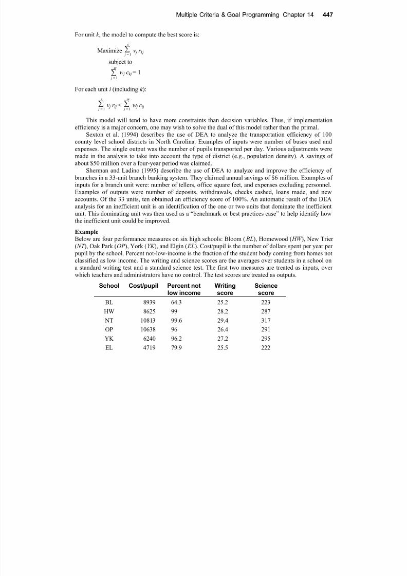
Below are four performance measures on six high schools: Bloom ( BL), Homewood ( HW ), New Trier( NT ), Oak Park (OP ), York (YK ), and Elgin ( EL). Cost/pupil is the number of dollars spent per year per
pupil by the school. Percent not-low-income is the fraction of the student body coming from homes notclassified as low income. The writing and science scores are the averages over students in a school ona standard writing test and a standard science test. The first two measures are treated as inputs, overwhich teachers and administrators have no control. The test scores are treated as outputs.
School Cost/pupil Percent notlow income
Writingscore
Sciencescore
BL 8939 64.3 25.2 223
HW 8625 99 28.2 287
NT 10813 99.6 29.4 317
OP 10638 96 26.4 291
YK 6240 96.2 27.2 295
EL 4719 79.9 25.5 222
448 Chapter 14 Multiple Criteria & Goal Programming

7/25/2019 Multiple Criteria and Goal Programming
http://slidepdf.com/reader/full/multiple-criteria-and-goal-programming 26/29
Which schools would you consider “efficient”? New Trier has the highest score in both writing
(29.4) and science (317). However, it also spends the most per pupil, $10,813, and has the highestfraction not-low-income. A DEA model for maximizing the score of New Trier appears below. Noticewe have scaled each factor, so it lies in the range (1,1000). This is important if one requires a strictly
positive minimum weight on each factor, as the last four constraints of the model imply. Themotivation for the strictly positive weight on each factor was given in the description of the“more-is- better” case:
MODEL:
MAX = SCORENT;
! Define the numerator for New Trier;
[DEFNUMNT] SCORENT - 317*WNTSCIN - 29.4*WNTWRIT = 0;
! Fix the denominator for New Trier;
[FIXDNMNT] 99.6*WNTRICH + 108.13*WNTCOST = 1;! Numerator/ Denominator < 1 for every school,;
! or equivalently, Numerator < Denominator;
[BLNT]223*WNTSCIN+25.2*WNTWRIT-64.3*WNTRICH-89.39*WNTCOST<=0;
[HWNT]287*WNTSCIN+28.2*WNTWRIT-99*WNTRICH-86.25*WNTCOST <= 0;
[NTNT]317*WNTSCIN+29.4*WNTWRIT-99.6*WNTRICH-108.13*WNTCOST<=0;
[OPNT]291*WNTSCIN+26.4*WNTWRIT-96*WNTRICH-106.38*WNTCOST<=0;
[YKNT]295*WNTSCIN+27.2*WNTWRIT-96.2*WNTRICH-62.40*WNTCOST<=0;
[ELNT]222*WNTSCIN+25.5*WNTWRIT-79.9*WNTRICH-47.19*WNTCOST<=0;
! Each measure must receive a little weight;
[SCINT] WNTSCIN >= 0.0005;
[WRINT] WNTWRIT >= 0.0005;
[RICNT] WNTRICH >= 0.0005;
[COSNT] WNTCOST >= 0.0005;
END
The solution is:
Optimal solution found at step: 3
Objective value: 0.9615803
Variable Value Reduced Cost
SCORENT 0.9615803 0.0000000
WNTSCIN 0.2987004E-02 0.0000000
WNTWRIT 0.5000000E-03 0.0000000
WNTRICH 0.8204092E-02 0.0000000
WNTCOST 0.1691228E-02 0.0000000
Row Slack or Surplus Dual Price
1 0.9615803 1.000000
DEFNUMNT 0.0000000 1.000000FIXDNMNT 0.0000000 0.9635345
BLNT 0.0000000 0.8795257
HWNT 0.8670327E-01 0.0000000
NTNT 0.3841965E-01 0.0000000
OPNT 0.8508738E-01 0.0000000
YKNT 0.0000000 0.4097145
ELNT 0.5945104E-01 0.0000000
SCINT 0.2487004E-02 0.0000000
WRINT 0.0000000 -3.908281
RICNT 0.7704092E-02 0.0000000
COSNT 0.1191227E-02 0.0000000
Multiple Criteria & Goal Programming Chapter 14 449

7/25/2019 Multiple Criteria and Goal Programming
http://slidepdf.com/reader/full/multiple-criteria-and-goal-programming 27/29
The score of New Trier is less than 1.0. Thus, according to DEA, New Trier is not efficient.Looking at the solution report, one can deduce that NT is, according to DEA, strictly less efficient than
BL and YK . Notice their “score less-than-or-equal-to 1” constraints are binding. Thus, if NT wants toimprove its efficiency by doing a benchmark study, it should perhaps study the practices of BL and YK
for insight.A sets-based model that evaluates all the schools in one model is given below:
MODEL:
! Data Envelopment Analysis of Decision Maker Efficiency ;
SETS:
DMU: !The decisionmaking units;
SCORE;! Each decision making unit has a
score to be computed;
FACTOR;
! There is a set of factors, input & output;
DXF( DMU, FACTOR): F, ! F( I, J) = Jth factor of DMU I;
W; ! Weights used to compute DMU I's score;
ENDSETS
DATA:
DMU = BL HW NT OP YK EL;
! Inputs are spending/pupil, % not low income;
! Outputs are Writing score and Science score;
NINPUTS = 2; ! The first NINPUTS factors are inputs;
FACTOR= COST RICH WRIT SCIN;! The inputs, the outputs;
F = 89.39 64.3 25.2 223
86.25 99 28.2 287
108.13 99.6 29.4 317
106.38 96 26.4 291
62.40 96.2 27.2 295
47.19 79.9 25.5 222;
WGTMIN = .0005; ! Min weight applied to every factor;
BIGM = 999999; ! Biggest a weight can be; ENDDATA
!----------------------------------------------------------;
! The Model;
! Try to make everyone's score as high as possible;
MAX = @SUM( DMU: SCORE);
! The LP for each DMU to get its score;
@FOR( DMU( I):
[CSCR] SCORE( I) = @SUM( FACTOR(J)|J #GT# NINPUTS:
F(I, J)* W(I, J));! Sum of inputs(denominator) = 1;
[SUM21] @SUM( FACTOR( J)| J #LE# NINPUTS:
F( I, J)* W( I, J)) = 1;
! Using DMU I's weights, no DMU can score better than 1,
Note Numer/Denom <= 1 implies Numer <= Denom;
@FOR( DMU( K):
[LE1] @SUM( FACTOR( J)| J #GT# NINPUTS: F( K, J) * W( I, J))
<= @SUM( FACTOR( J)| J #LE# NINPUTS: F( K, J) * W( I, J))
)
);
! The weights must be greater than zero;
450 Chapter 14 Multiple Criteria & Goal Programming

7/25/2019 Multiple Criteria and Goal Programming
http://slidepdf.com/reader/full/multiple-criteria-and-goal-programming 28/29
@FOR( DXF( I, J): @BND( WGTMIN, W, BIGM));
END
Part of the output is:
Variable Value Reduced CostSCORE( BL) 1.000000 0.0000000
SCORE( HW) 0.9095071 0.0000000
SCORE( NT) 0.9615803 0.0000000
SCORE( OP) 0.9121280 0.0000000
SCORE( YK) 1.000000 0.0000000
SCORE( EL) 1.000000 0.0000000
We see that the only efficient schools are Bloom, Yorktown, and Elgin.
14.7 Problems1. In the example staffing problem in this chapter, the primary criterion was minimizing the number
of people hired. The secondary criterion was to spread out any excess capacity as much as possible. The primary criterion received a weight of 9; whereas, the secondary criterion received aweight of 1. The minimum number of people required (primary criterion) was 8. How much couldthe weight on the secondary criterion be increased before the number of people hired increases tomore than 8?
2. Reconsider the advertising media selection problem of this chapter.
a) Reformulate it, so we achieve at least 197 (in 1000’s) useful exposures at minimum cost.
b) Predict the cost before looking at the solution.
3. A description of a “project crashing” decision appears in Chapter 8. There were two criteria,
project length and project cost. Trace out the efficient frontier describing the trade-off betweenlength and cost.
4. The various capacities of several popular sport utility vehicles, as reported by a popular consumerrating magazine, are listed below:
Vehicle SeatsCargo FloorLength (in.)
Rear OpeningHeight (in.)
Cargo Volume(cubic ft)
Blazer 6 75.5 31.5 42.5
Cherokee 5 62.0 33.5 34.5
Land Rover 7 49.5 42.0 42.0
Land Cruiser 8 65.5 38.5 44.5Explorer 6 78.5 35.0 48.0
Trooper 5 57.0 36.5 42.5
Multiple Criteria & Goal Programming Chapter 14 451
7/25/2019 Multiple Criteria and Goal Programming
http://slidepdf.com/reader/full/multiple-criteria-and-goal-programming 29/29
Assuming sport utility vehicle buyers sport a linear utility and more capacity is better, whichof the above vehicles are on the efficient frontier according to these four capacity measures?
5. The Rotorua Fruit Company sells various kinds of premium fruits (e.g., apples, peaches, and kiwi
fruit) in small boxes. Each box contains a single kind of fruit. The outside of the box specifies:i) the kind of fruit,
ii) the number of pieces of fruit, and
iii) the approximate weight of the fruit in the box.
Satisfying specification (iii) is nontrivial, because the per unit weight of fruit as it comes fromthe orchard is a random variable. Consider the case of apples. Each apple box contains 12 apples.The label on each apple box says the box contains 4.25 lbs. of apples. In fact, a typical apple
weighs from 5 to 6.5 ounces. At 16 ounces/lb., a box of 5-ounce apples would weigh only 3.75lbs., whereas, a box of 6.5-ounce apples would weigh 4.875 lbs. The approach Rotorua isconsidering is to have a set of 24 automated scales on the box loading line. The 24 scales will beloaded with 24 apples. Based on the weights of the apples, a set of 12 apples whose total weightcomes close to 4.25 lbs., will be dropped into the current empty box. In the next cycle, the 12empty scales will be reloaded with new apples, a new empty box will be moved into position, andthe process repeated. Rotorua cannot always achieve the ideal of exactly 4.25 lbs. in a box.However, being underweight is worse than being overweight. Rotorua has characterized itsfeeling/utility for this under/over issue by stating that given the choice between loading a box oneounce under and one ounce over, it clearly prefers to load it one ounce over. However, it would beindifferent between loading a box one ounce under vs. five ounces over.
Suppose the scales currently contain apples with the following weights in ounces:
5.6, 5.9, 6.0, 5.8, 5.9, 5.4, 5.0, 5.5, 6.3, 6.2, 5.1, 6.2,
6.1, 5.2, 6.4, 5.7, 5.6, 5.5, 5.3, 6.0, 5.4, 5.3, 5.8, 6.1.
a) How would you load the next box?
b) Discuss some of the issues in implementing your approach.


