Multiple-Choice Test Parabolic Partial Differential Equations
15
Multiple-Choice Test Parabolic Partial Differential Equations Partial Differential Equations COMPLETE SOLUTION SET 1. In a general second order linear partial differential equation with two independent variables 0 2 2 2 2 2 = + ∂ ∂ + ∂ ∂ ∂ + ∂ ∂ D y u C y x u B x u A where A , B , C are functions of x and y , and D is a function of x , y , x u ∂ ∂ , y u ∂ ∂ , then the partial differential equation is parabolic if (A) 0 4 2 < − AC B (B) 0 4 2 > − AC B (C) 0 4 2 = − AC B (D) 0 4 2 ≠ − AC B Solution The correct answer is (C). A general second order linear partial differential equation is parabolic if 0 4 2 = − AC B .
Transcript of Multiple-Choice Test Parabolic Partial Differential Equations

Multiple-Choice Test Parabolic Partial Differential Equations Partial Differential Equations COMPLETE SOLUTION SET 1. In a general second order linear partial differential equation with two independent
variables
02
22
2
2
=+∂∂
+∂∂
∂+
∂∂ D
yuC
yxuB
xuA
where A , B , C are functions of x and y , and D is a function of x , y , xu∂∂ ,
yu∂∂ , then
the partial differential equation is parabolic if (A) 042 <− ACB (B) 042 >− ACB (C) 042 =− ACB (D) 042 ≠− ACB
Solution The correct answer is (C). A general second order linear partial differential equation is parabolic if 042 =− ACB .

2. The region in which the following partial differential equation
053272
2
2
2
23 =+
∂∂∂
+∂∂
+∂∂ u
yxu
yu
xux
acts as parabolic equation is
(A) 3/1
121
>x
(B) 3/1
121
<x
(C) for all values of x
(D) 3/1
121
=x
Solution The correct answer is (D). A general partial differential equation with two independent variables is of the form
02
22
2
2
=+∂∂
+∂∂
+∂∂ D
yuC
xyuB
xuA
where CBA and,, are functions of yx and and is a function of yu
xuuyx
∂∂
∂∂ ,and,, .
For this equation to be parabolic, 042 =− ACB . In the above question, 27,3,3 === CBxA , giving
3/1
3
3
3
3
32
2
121
121
1089
910801089
0)27)((4)3(04
=
=
=
=
=−
=−
=−
x
x
x
xx
xACB

3. The partial differential equation of the temperature in a long thin rod is given by
2
2
xT
tT
∂∂
=∂∂ α
If scm /8.0 2=α , the initial temperature of rod is C°40 , and the rod is divided into three equal segments, the temperature at node 1 (using st 1.0=∆ ) by using an explicit solution at sec2.0=t is
(A) 40.7134 C0 (B) 40.6882 C0 (C) 40.7033 C0 (D) 40.6956 C0
Solution The correct answer is (C). Given
scm /8.0 2=α st 1.0=∆
st sec2.0= cms9=L
Number of divisions of the rod, 3=n
339
=
=
=∆nLx
Number of time steps=ttt initialfinal
∆
−
1.0
02.0 −=
2=
( )2xt
∆∆
=αλ
0=node 1 2 3
cm9
CT °= 20CT °= 80

( )23
1.08.0=
0089.0= The boundary conditions
1,0allfor20
80
3
0 =
°=
°=j
CTCT
j
j
(E3.1)
The initial temperature of the rod is C°40 , that is, all the temperatures of the nodes inside the rod are at C°40 when time, sec0=t except for the boundary nodes as given by Equation (E3.1). This could be represented as
1,2 allfor ,200 =°= iCTi . (E3.2) Initial temperature at the nodes inside the rod (when t=0 sec)
(E3.1)Equationfrom8000 CT °=
(E3.2)Equationfrom40
400
2
01
°=
°=
CTCT
(E3.1)Equationfrom2003 CT °=
Temperature at the nodes inside the rod when t=0.1 sec Setting 0=j and 3,2,1,0=i in Equation (7) (from Chapter 10.02) gives the temperature of the nodes inside the rod when time, sec1.0=t .
(E3.1)ConditionBoundary8010 CT °=
( )
( )( )
C
TTTTT
°=+=+=
+−+=+−+=
3556.403556.040
400089.04080)40(2400089.040
2 00
01
02
01
11 λ
( )
( )( )
C
TTTTT
°=−=
−+=+−+=
+−+=
8222.391778.040
200089.04040)40(2200089.040
2 01
02
03
02
12 λ
(E3.1)ConditionBoundary201
3 CT °=

Temperature at the nodes inside the rod when t=0.2 sec Setting 1=j and 3,2,1,0=i in Equation (6) (from Chapter 11.02) gives the temperature of the nodes inside the rod when time, sec2.0=t
(E3.1)ConditionBoundary8020 CT °=
( )
( )( )
C
TTTTT
°=+=+=
+−+=+−+=
7033.403477.03556.40
1110.390089.03556.4080)3556.40(28222.390089.03556.40
2 10
11
12
11
21 λ
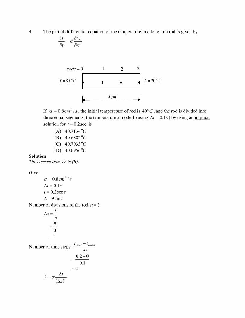
4. The partial differential equation of the temperature in a long thin rod is given by
2
2
xT
tT
∂∂
=∂∂ α
If scm /8.0 2=α , the initial temperature of rod is C°40 , and the rod is divided into three equal segments, the temperature at node 1 (using st 1.0=∆ ) by using an implicit solution for sec2.0=t is
(A) 40.7134 C0 (B) 40.6882 C0 (C) 40.7033 C0 (D) 40.6956 C0
Solution The correct answer is (B). Given
scm /8.0 2=α st 1.0=∆
st sec2.0= cms9=L
Number of divisions of the rod, 3=n
339
=
=
=∆nLx
Number of time steps=ttt initialfinal
∆
−
1.0
02.0 −=
2=
( )2xt
∆∆
=αλ
0=node 1 2 3
cm9
CT °= 20CT °= 80

( )23
1.08.0=
0089.0= The boundary conditions
1,0allfor20
80
3
0 =
°=
°=j
CTCT
j
j
(E4.1)
The initial temperature of the rod is C°40 , that is, all the temperatures of the nodes inside the rod are at C°40 when time, sec0=t except for the boundary nodes as given by Equation (E3.1). This could be represented as
1,2 allfor ,200 =°= iCTi . (E4.2) Initial temperature at the nodes inside the rod (when t=0 sec)
(E4.1)Equationfrom8000 CT °=
(E4.2)Equationfrom40
400
2
01
°=
°=
CTCT
(E4.1)Equationfrom2003 CT °=
Temperature at the nodes inside the rod when t=0.1 sec
(E4.1)ConditionBoundary20
801
3
10
°=
°=
CTCT
For all the interior nodes, putting 0=j and 2,1=i in Equation (11) (from Chapter 10.02) gives the following equations i=1
400089.00178.17111.0
40)0089.0()0089.021()800089.0(
)21(
12
11
12
11
01
12
11
10
=−+−
=−×++×−
=−++−
TTTT
TTTT λλλ
7111.400089.00178.1 12
11 =− TT (E4.3)
i=2 0
21
312
11 )21( TTTT =−++− λλλ
40)200089.0(0178.10089.0 12
11 =×−+− TT
401778.00178.10089.0 12
11 =−+− TT
1778.400178.10089.0 12
11 =+− TT (E4.4)
The simultaneous linear equations (E4.3) – (E4.4) can be written in matrix form as
=
−
−1778.407111.40
0178.10089.00089.00178.1
12
11
TT
The above coefficient matrix is tri-diagonal. Special algorithms such as Thomas’ algorithm can be used to solve simultaneous linear equation with tri-diagonal coefficient matrices. The solution is given by

=
8284.393478.40
12
11
TT
Temperature at the nodes inside the rod when t=0.2 sec
(E4.1)ConditionBoundary20
802
3
20
°=
°=
CTCT
For all the interior nodes, putting 1=j and 2,1=i in Equation (11) (from Chapter 10.02) gives the following equations i=1
3478.400089.00178.17111.0
3478.400089.0)0089.021()800089.0(
)21(
22
21
22
21
11
22
21
20
=−+−
=−×++×−
=−++−
TTTT
TTTT λλλ
0590.410089.00178.1 22
21 =− TT (E4.5)
i=2 1
22
32
22
1 )21( TTTT =−++− λλλ 8284.39)200089.0(0178.10089.0 2
22
1 =×−+− TT 8284.391778.00178.10089.0 2
22
1 =−+− TT 0061.400178.10089.0 2
22
1 =+− TT (E4.6) The simultaneous linear equations (E4.5) – (E4.6) can be written in matrix form as
=
−
−0061.400590.41
0178.10089.00089.00178.1
22
21
TT
The above coefficient matrix is tri-diagonal. Special algorithms such as Thomas’ algorithm can be used to solve simultaneous linear equation with tri-diagonal coefficient matrices. The solution is given by
=
6627.396882.40
22
21
TT

5. The partial differential equation of the temperature in a long thin rod is given by
2
2
xT
tT
∂∂
=∂∂ α
If scm /8.0 2=α , the initial temperature of rod is C°40 , and the rod is divided into three equal segments, the temperature at node 1 (using st 1.0=∆ ) by using a Crank-Nicolson solution for sec2.0=t is
(A) 40.7134 C0 (B) 40.6882 C0 (C) 40.7033 C0 (D) 40.6956 C0
Solution The correct answer is (D). Given
scm /8.0 2=α st 1.0=∆
st sec2.0= cms9=L
Number of divisions of the rod, 3=n
339
=
=
=∆nLx
Number of time steps=ttt initialfinal
∆
−
1.0
02.0 −=
2=
( )2xt
∆∆
=αλ
0=node 1 2 3
cm9
CT °= 20CT °= 80

( )23
1.08.0=
0089.0= The boundary conditions
1,0allfor20
80
3
0 =
°=
°=j
CTCT
j
j
(E5.1)
The initial temperature of the rod is C°40 , that is, all the temperatures of the nodes inside the rod are at C°40 when time, sec0=t except for the boundary nodes as given by Equation (E5.1). This could be represented as
1,2 allfor ,200 =°= iCTi . (E5.2) Initial temperature at the nodes inside the rod (when t=0 sec)
(E4.1)Equationfrom8000 CT °=
(E4.2)Equationfrom40
400
2
01
°=
°=
CTCT
(E4.1)Equationfrom2003 CT °=
Temperature at the nodes inside the rod when t=0.1 sec
(E4.1)ConditionBoundary20
801
3
10
°=
°=
CTCT
For all the interior nodes, putting 0=j and 2,1=i in Equation (15) (from Chapter 10.02) gives the following equations i=1
3556.02889.797111.00089.00178.27111.0
40)0089.0(40)0089.01(280)0089.0(0089.0)0089.01(2)800089.0(
)1(2)1(2
12
11
12
11
02
01
00
12
11
10
++=−+−
+−+=−++×−
+−+=−++−
TTTT
TTTTTT λλλλλλ
0667.810089.00178.2 12
11 =− TT (E5.3)
i=2
20)0089.0(40)0089.01(240)0089.0()200089.0()0089.01(20089.0
)1(2)1(21
21
1
03
02
01
13
12
11
+−+=×−++−
+−+=−++−
TTTTTTTT λλλλλλ
1778.02889.793556.01778.00178.20089.0 12
11 ++=−+− TT
0000.800178.20089.0 12
11 =+− TT (E5.4)
The simultaneous linear equations (E5.3) – (E4.4) can be written in matrix form as
=
−
−0000.800667.81
0178.20089.00089.00178.2
12
11
TT
The above coefficient matrix is tri-diagonal. Special algorithms such as Thomas’ algorithm can be used to solve simultaneous linear equation with tri-diagonal coefficient matrices. The solution is given by

=
8253.393517.40
12
11
TT
Temperature at the nodes inside the rod when t=0.2 sec
(E4.1)ConditionBoundary20
802
3
20
°=
°=
CTCT
For all the interior nodes, putting 1=j and 2,1=i in Equation (11) (from Chapter 10.02) gives the following equations i=1
3540.09860.797111.00089.00178.27111.08253.39)0089.0(3517.40)00899.01(280)0089.0(
0089.0)0089.01(2)800089.0(
)1(2)1(2
22
21
22
21
12
11
10
22
21
20
++=−+−
+−+=−++×−
+−+=−++−
TT
TTTTTTTT λλλλλλ
7622.810089.00178.2 22
21 =− TT (E5.5)
i=2
1780.09426.783587.01780.00178.20089.020)0089.0(8253.39)0089.01(23517.40)0089.0(
)200089.0()0089.01(20089.0
)1(2)1(2
22
21
22
21
13
12
11
23
22
21
++=−+−
+−+=×−++−
+−+=−++−
TT
TTTTTTTT λλλλλλ
6569.790178.20089.0 22
21 =+− TT (E5.6)
The simultaneous linear equations (E5.5) – (E5.6) can be written in matrix form as
=
−
−6569.797622.81
0178.20089.00089.00178.2
22
21
TT
The above coefficient matrix is tri-diagonal. Special algorithms such as Thomas’ algorithm can be used to solve simultaneous linear equation with tri-diagonal coefficient matrices. The solution is given by
=
6568.396956.40
22
21
TT

6. The partial differential equation of the temperature in a long thin rod is given by
2
2
xT
tT
∂∂
=∂∂ α
If scm /8.0 2=α , the initial temperature of rod is C°40 , and the rod is divided into three equal segments, the temperature at node 1 (using st 1.0=∆ ) by using an explicit
solution at sec2.0=t is. (For node 0, )( 0TThxTk a −=∂∂
− ), where
)/(9 CmWk °= , 2/20 mWh = , CTa °= 25 , =0T the temperature of rod at node 0 (A) 41.6478 C0 (B) 38.4356 C0 (C) 39.9983 C0 (D) 37.5798 C0
Solution The correct answer is (C). Given
scm /8.0 2=α st 1.0=∆
st sec2.0= cms9=L
CTa °= 25 2/20 mWh =
)/(9 CmWk °= Number of divisions of the rod, 3=n
cm
nLx
339
=
=
=∆
0=node 1 2 3
cm9
CT °= 20insulated

Number of time steps=ttt initialfinal
∆
−
1.0
02.0 −=
2=
( )2xt
∆∆
=αλ
( )23
1.08.0=
0089.0= The boundary conditions
1,0allfor0),(
20
,,
3
=
=−=∂∂
−
°=j
iTThxTk
CT
jiaji
j
(E6.1)
Approximating the derivative by the central divided difference,
)(211
, xTT
xT j
ij
i
ji ∆−
≅∂∂ −+ (E6.2)
Substituting Equation (E6.2) in the derivative boundary condition of Equation (E6.3) we have
0),()(2
11 =−=
∆−
− −+ iTThxTTk j
ia
ji
ji
Rewriting the above equation we have
0,)(2 11 =+−∆= +− iTTTxkhT j
ij
iaj
i (E6.4)
From the explicit method (Equation 7 from Chapter 10.02) we have ( ) 0,2 11
1 ≠+−+= −++ iTTTTT j
ij
ij
ij
ij
i λ (E6.5) Substituting Equation (E6.4) in Equation (E6.5) we get
+−∆+−+= ++
+ ji
jia
ji
ji
ji
ji TTTx
khTTTT 11
1 )(22λ
0,)(2 1 =
−∆+−+= + iTTx
khTTT j
iaj
ij
ij
i λ (E6.8)
Equation (E6.8) is used for the node 0 (insulated edge) The initial temperature of the rod is C°40 , that is, all the temperatures of the nodes inside the rod are at C°40 when time, sec0=t except for the boundary nodes as given by Equation (E6.1). This could be represented as
1,2,3 allfor ,200 =°= iCTi . (E6.9) Initial temperature at the nodes inside the rod (when t=0 sec)
(E6.9)Equationfrom
40
40
40
02
01
00
°=
°=
°=
CTCTCT

(E6.1)Equationfrom2003 CT °=
Temperature at the nodes inside the rod when t=0.1 sec Setting 0=j and 3,2,1,0=i in Equation (7) (from Chapter 10.02) gives the temperature of the nodes inside the rod when time, sec1.0=t . i=0
−∆+−+= )(2 0
00
00
10
01
0 TTxkhTTTT aλ (From Equation E6.8)
−+−×+= )4025(03.0
92040400089.0240 note: mx 03.0=∆
( )1017778.040 −+= 017778.040 −=
C°= 9822.39 i=1
( )( )( )
C
TTTTT
°=+=+=
+−+=+−+=
0000.40040
00089.04040)40(2400089.040
2 00
01
02
01
11 λ
i=2 ( )
( )( )
C
TTTTT
°=−=
−+=+−+=
+−+=
8222.391778.040
200089.04040)40(2200089.040
2 01
02
03
02
12 λ
i=3
(E3.1)ConditionBoundary2013 CT °=

Temperature at the nodes inside the rod when t=0.2 sec Setting 1=j and 3,2,1,0=i in Equation (7) (from Chapter 10.02) gives the temperature of the nodes inside the rod when time, sec2.0=t i=0
−∆+−+= )(2 1
01
01
11
02
0 TTxkhTTTT aλ (From Equation E6.8)
−+−×+= )9822.3925(03.0
9209822.39400089.029822.39 note : mx 03.0=∆
( )98101.0017778.09822.39 −+= 01744.09822.39 −=
C°= 9648.39 i=1
( )( )( )
C
TTTTT
°=−=
−+=+−+=
+−+=
9983.39001741.00000.40
1956.00089.00000.409822.39)0000.40(28222.390089.00000.40
2 10
11
12
11
21 λ


![Neumann Boundary Problem for Parabolic Partial Differential … · 2018-08-06 · arXiv:1802.07626v1 [math.PR] 21 Feb 2018 Neumann Boundary Problem for Parabolic Partial Differential](https://static.fdocuments.net/doc/165x107/5fad472c1e274c0e81441004/neumann-boundary-problem-for-parabolic-partial-differential-2018-08-06-arxiv180207626v1.jpg)