Multiphase Turbulent Flow

Ken Kiger - UMCP

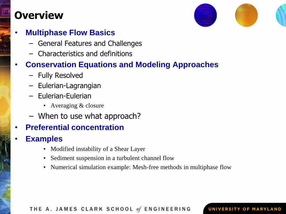
Overview

• Multiphase Flow Basics

– General Features and Challenges

– Characteristics and definitions

• Conservation Equations and Modeling Approaches

– Fully Resolved

– Eulerian-Lagrangian

– Eulerian-Eulerian

• Averaging & closure

– When to use what approach?

• Preferential concentration

• Examples

• Modified instability of a Shear Layer

• Sediment suspension in a turbulent channel flow

• Numerical simulation example: Mesh-free methods in multiphase flow

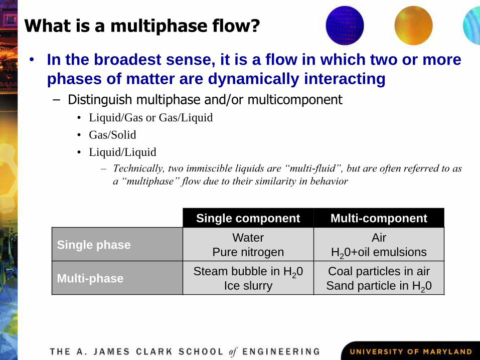
What is a multiphase flow?

• In the broadest sense, it is a flow in which two or more

phases of matter are dynamically interacting

– Distinguish multiphase and/or multicomponent

• Liquid/Gas or Gas/Liquid

• Gas/Solid

• Liquid/Liquid

– Technically, two immiscible liquids are “multi-fluid”, but are often referred to as

a “multiphase” flow due to their similarity in behavior

Single component Multi-component

Single phaseWater

Pure nitrogen

Air

H20+oil emulsions

Multi-phaseSteam bubble in H20

Ice slurry

Coal particles in air

Sand particle in H20

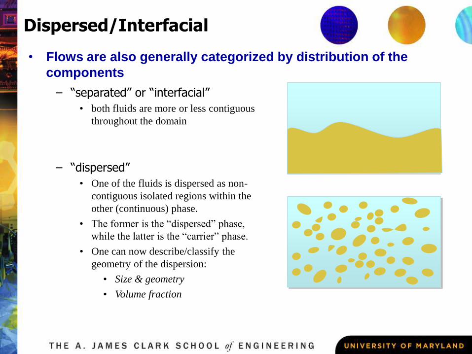
Dispersed/Interfacial

• Flows are also generally categorized by distribution of the

components

– “separated” or “interfacial”

• both fluids are more or less contiguous

throughout the domain

– “dispersed”

• One of the fluids is dispersed as non-

contiguous isolated regions within the

other (continuous) phase.

• The former is the “dispersed” phase,

while the latter is the “carrier” phase.

• One can now describe/classify the

geometry of the dispersion:

• Size & geometry

• Volume fraction

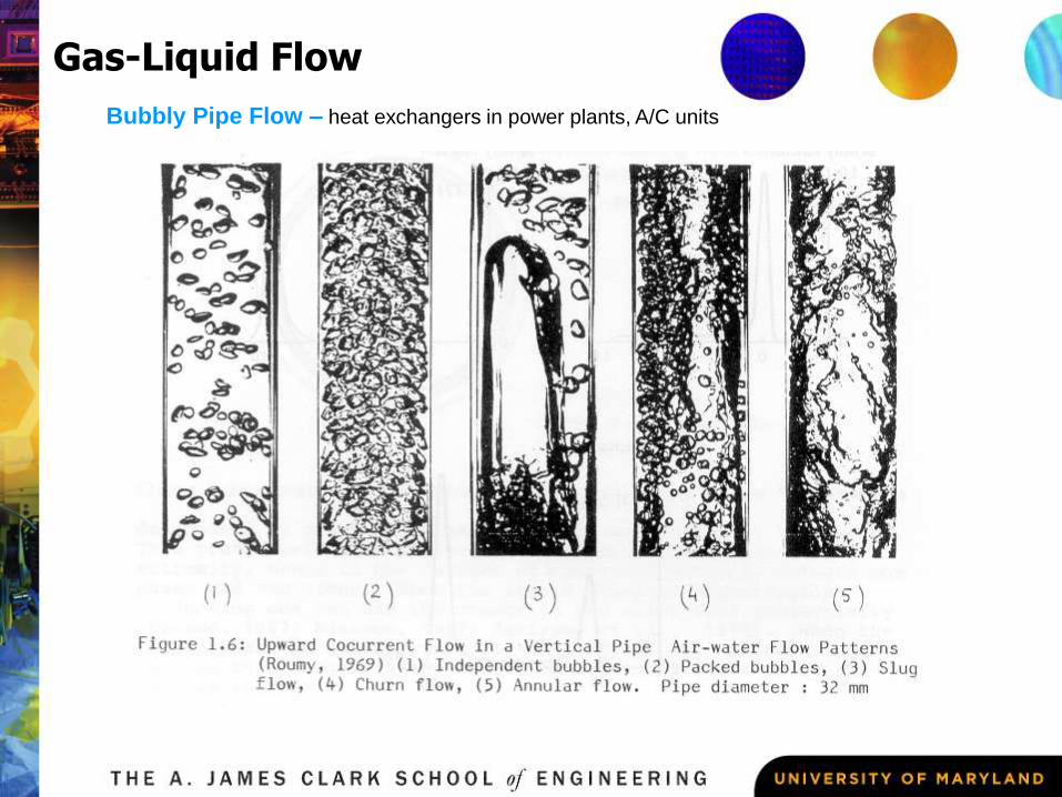
Bubbly Pipe Flow – heat exchangers in power plants, A/C units

Gas-Liquid Flow

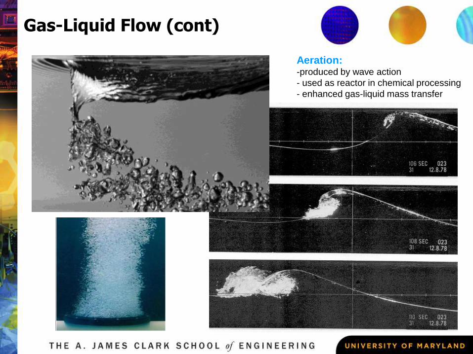
Aeration:-produced by wave action

- used as reactor in chemical processing

- enhanced gas-liquid mass transfer

Gas-Liquid Flow (cont)

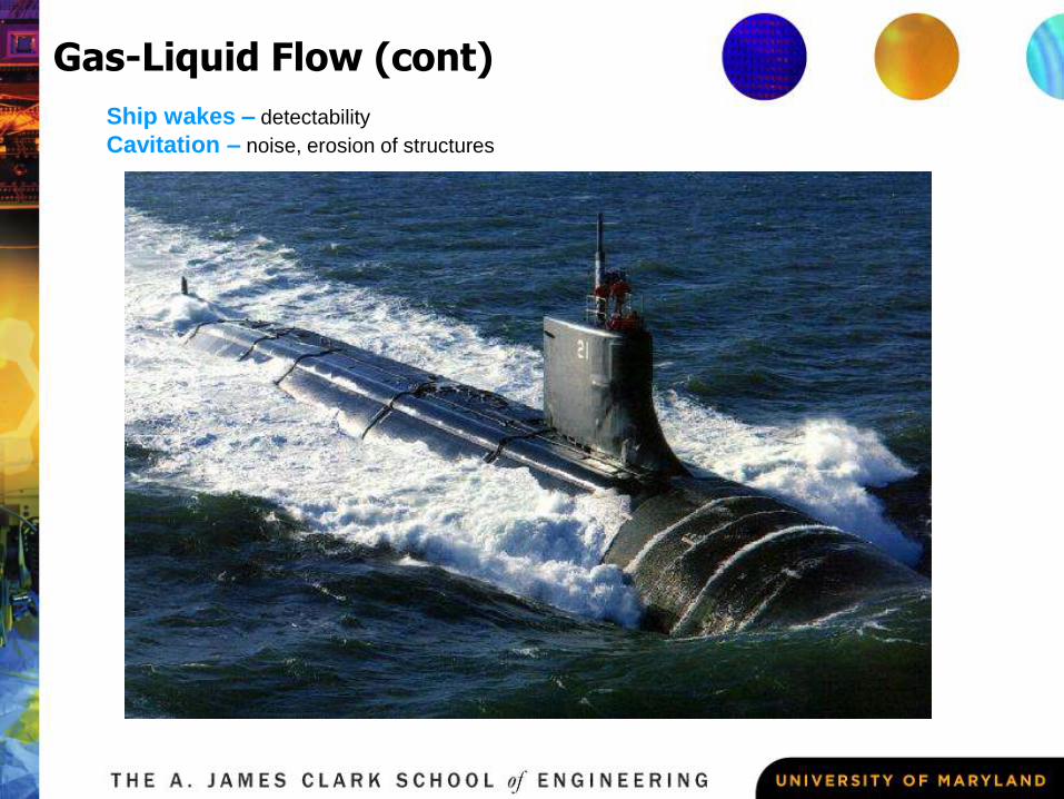
Ship wakes – detectability

Cavitation – noise, erosion of structures

Gas-Liquid Flow (cont)

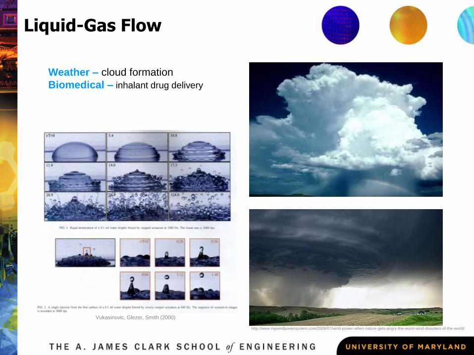
Weather – cloud formation

Biomedical – inhalant drug delivery

Liquid-Gas Flow

http://www.mywindpowersystem.com/2009/07/wind-power-when-nature-gets-angry-the-worst-wind-disasters-of-the-world/

Vukasinovic, Glezer, Smith (2000)

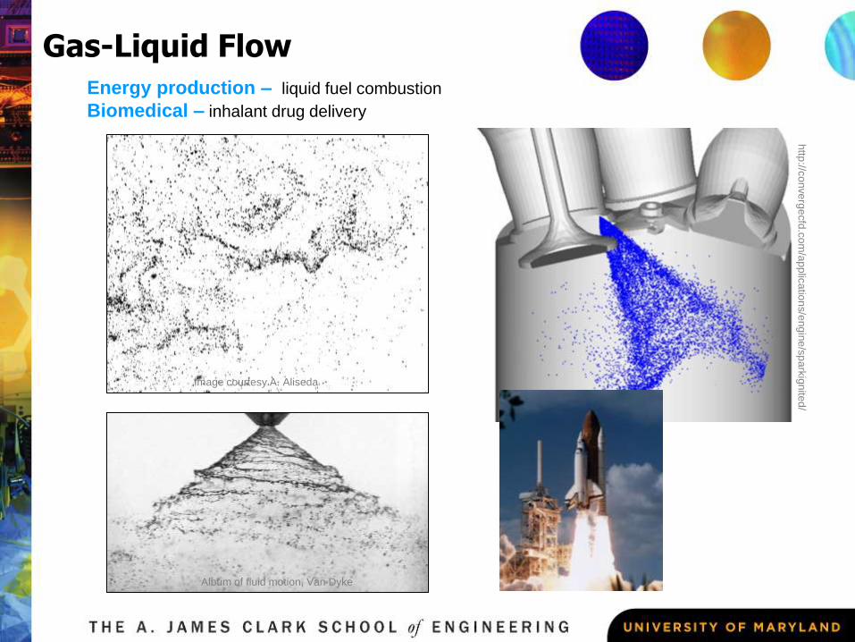
Energy production – liquid fuel combustion

Biomedical – inhalant drug delivery

Gas-Liquid Flowh

ttp://c

on

ve

rge

cfd

.co

m/a

pp

lica

tion

s/e

ng

ine

/sp

ark

ign

ited

/

Album of fluid motion, Van Dyke

Image courtesy A. Aliseda

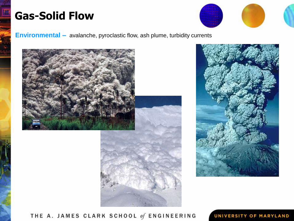
Gas-Solid Flow

Environmental – avalanche, pyroclastic flow, ash plume, turbidity currents

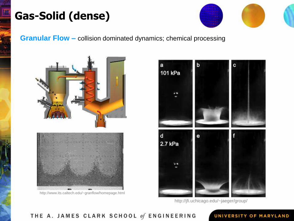
Gas-Solid (dense)

Granular Flow – collision dominated dynamics; chemical processing

http://jfi.uchicago.edu/~jaeger/group/

http://www.its.caltech.edu/~granflow/homepage.html

Chemical production – mixing and reaction of immiscible liquids

http://www.physics.emory.edu/students/kdesmond/2DEmulsion.html

Liquid-Liquid

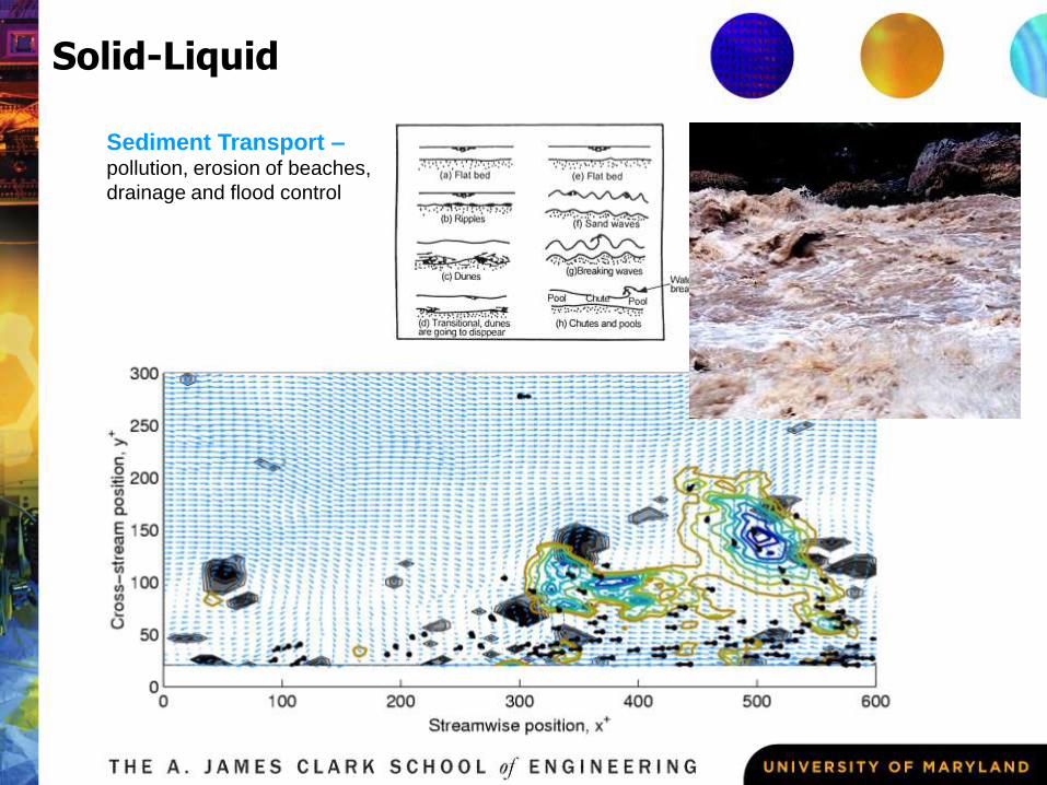
Sediment Transport –pollution, erosion of beaches,

drainage and flood control

Solid-Liquid

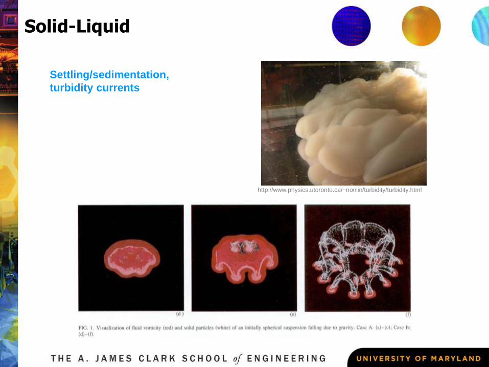
Settling/sedimentation,

turbidity currents

Solid-Liquid

http://www.physics.utoronto.ca/~nonlin/turbidity/turbidity.html

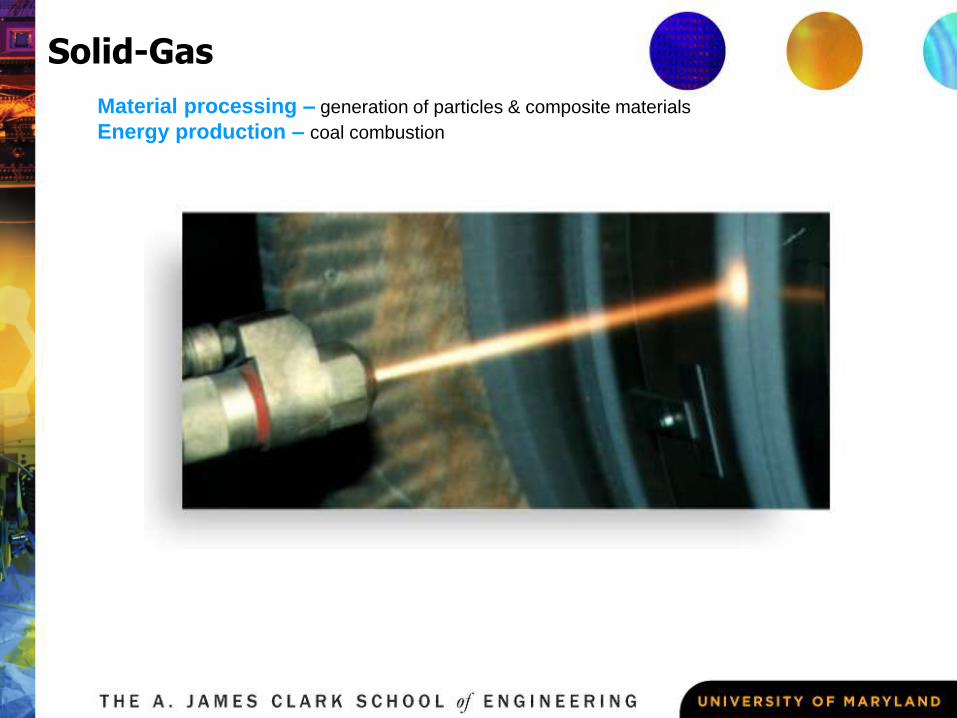
Material processing – generation of particles & composite materials

Energy production – coal combustion

Solid-Gas

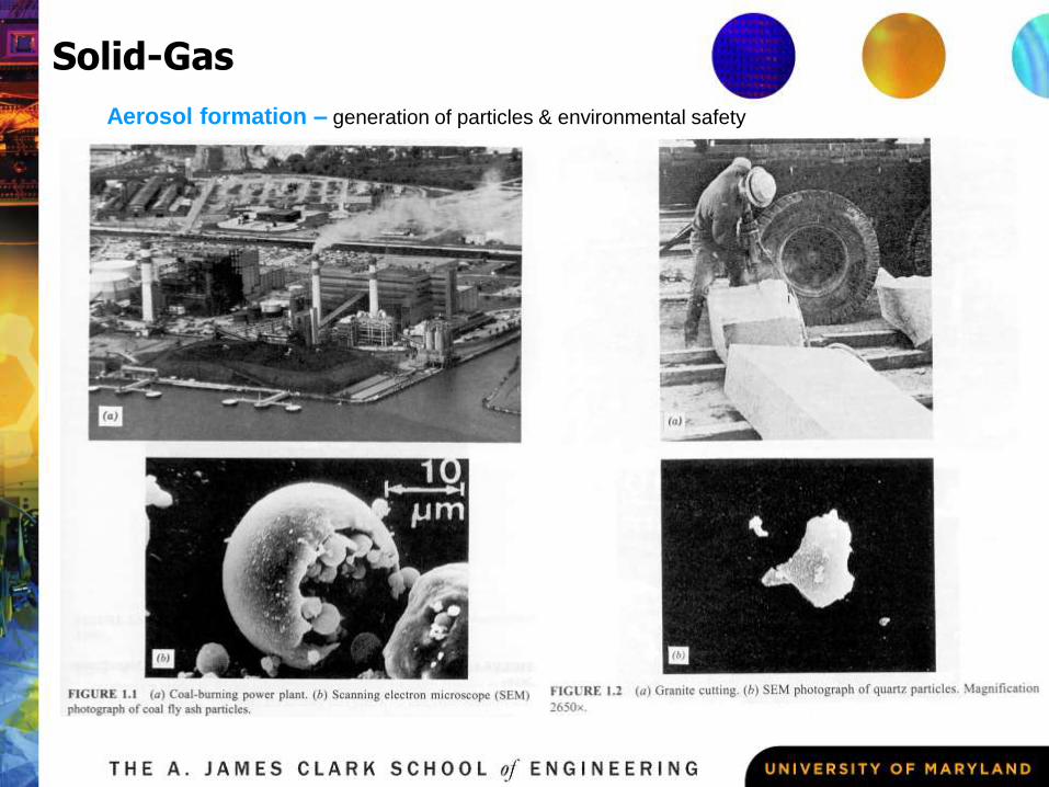
Aerosol formation – generation of particles & environmental safety

Solid-Gas

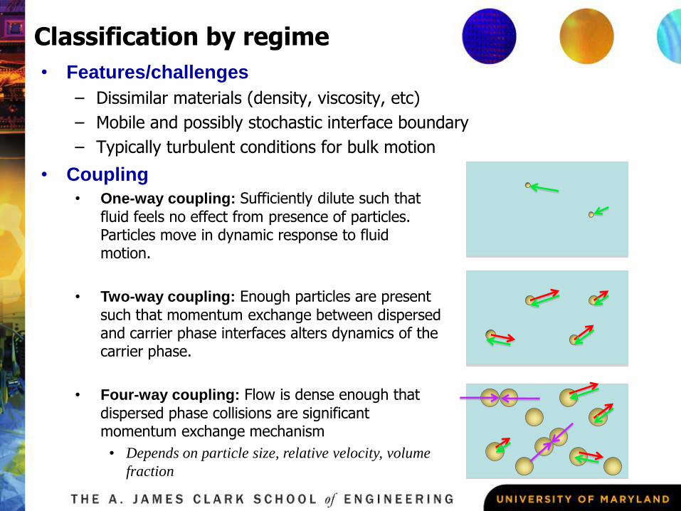
Classification by regime

• Features/challenges

– Dissimilar materials (density, viscosity, etc)

– Mobile and possibly stochastic interface boundary

– Typically turbulent conditions for bulk motion

• Coupling

• One-way coupling: Sufficiently dilute such that

fluid feels no effect from presence of particles. Particles move in dynamic response to fluid motion.

• Two-way coupling: Enough particles are present

such that momentum exchange between dispersed and carrier phase interfaces alters dynamics of the carrier phase.

• Four-way coupling: Flow is dense enough that

dispersed phase collisions are significant momentum exchange mechanism

• Depends on particle size, relative velocity, volume

fraction

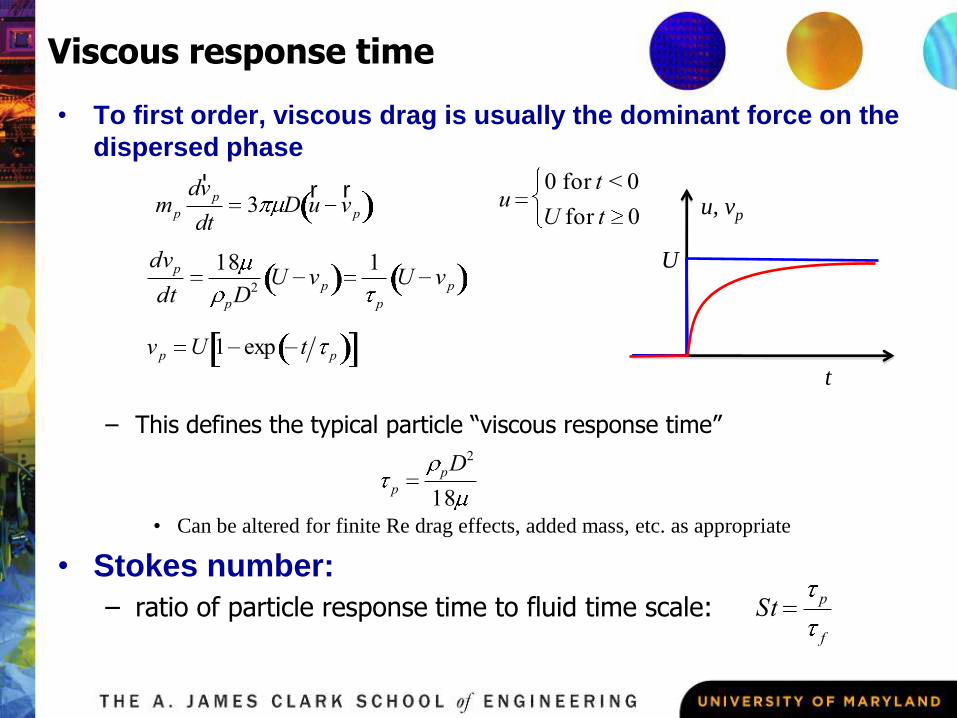
Viscous response time

• To first order, viscous drag is usually the dominant force on the

dispersed phase

– This defines the typical particle “viscous response time”

• Can be altered for finite Re drag effects, added mass, etc. as appropriate

• Stokes number:

– ratio of particle response time to fluid time scale:

mp

dr v p

dt3 D

r u

r v p

u0 for t < 0

U for t 0

dvp

dt

18

pD2U vp

1

p

U vp

v p U 1 exp t p

u, vp

t

U

p

pD2

18

Stp

f

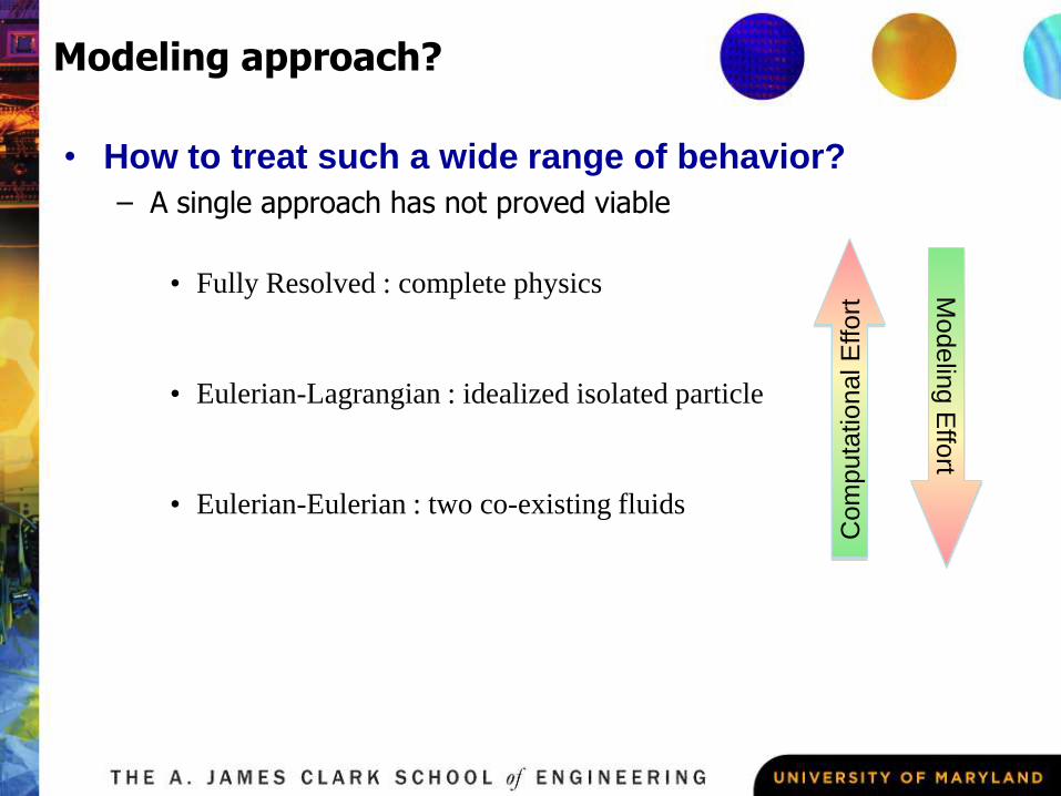
Modeling approach?

• How to treat such a wide range of behavior?

– A single approach has not proved viable

• Fully Resolved : complete physics

• Eulerian-Lagrangian : idealized isolated particle

• Eulerian-Eulerian : two co-existing fluids

Com

puta

tional E

ffort

Modelin

g E

ffort

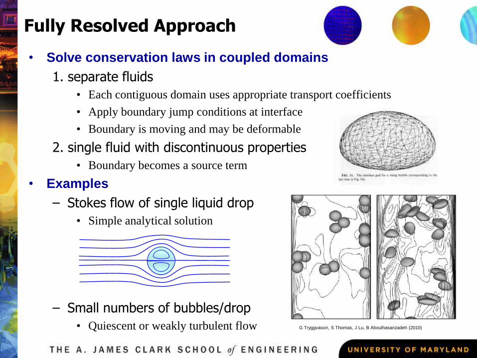
Fully Resolved Approach

• Solve conservation laws in coupled domains

1. separate fluids

• Each contiguous domain uses appropriate transport coefficients

• Apply boundary jump conditions at interface

• Boundary is moving and may be deformable

2. single fluid with discontinuous properties

• Boundary becomes a source term

• Examples

– Stokes flow of single liquid drop

• Simple analytical solution

– Small numbers of bubbles/drop

• Quiescent or weakly turbulent flow G Tryggvason, S Thomas, J Lu, B Aboulhasanzadeh (2010)

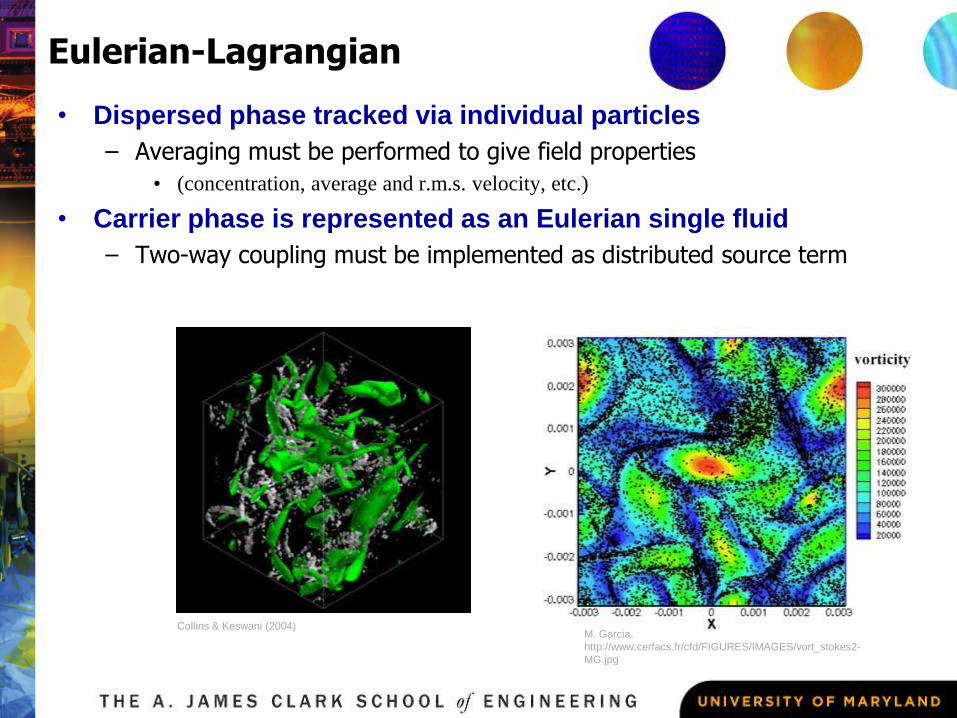
Eulerian-Lagrangian

• Dispersed phase tracked via individual particles

– Averaging must be performed to give field properties

• (concentration, average and r.m.s. velocity, etc.)

• Carrier phase is represented as an Eulerian single fluid

– Two-way coupling must be implemented as distributed source term

M. Garcia,

http://www.cerfacs.fr/cfd/FIGURES/IMAGES/vort_stokes2-

MG.jpg

Collins & Keswani (2004)

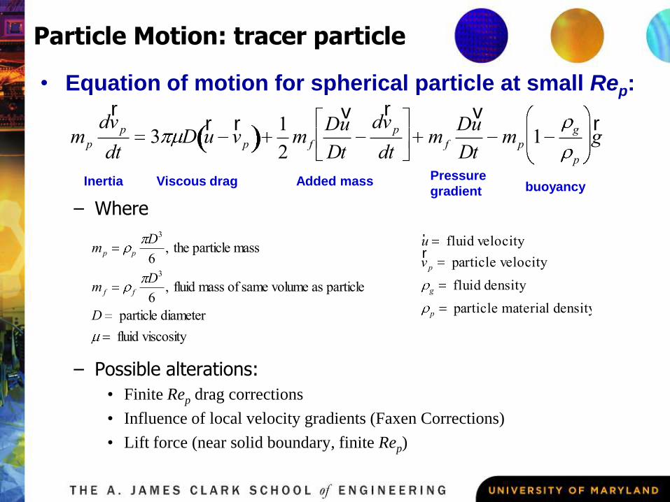
Particle Motion: tracer particle

• Equation of motion for spherical particle at small Rep:

– Where

– Possible alterations:

• Finite Rep drag corrections

• Influence of local velocity gradients (Faxen Corrections)

• Lift force (near solid boundary, finite Rep)

mp

dr v p

dt3 D

r u

r v p

1

2m f

Dv u

Dt

dr v p

dtm f

Dv u

Dtmp 1

g

p

r g

mp p

D3

6, the particle mass

m f f

D3

6, fluid mass of same volume as particle

D particle diameter

fluid viscosity

Added massViscous drag Pressure

gradient buoyancyInertia

r u fluid velocityr v p particle velocity

g fluid density

p particle material density

Two-Fluid Equations

• Apply averaging operator to mass and momentum equations

– Drew (1983), Simonin (1991)

• Phase indicator function

• Averaging operator

– Assume no inter-phase mass flux, incompressible carrier phase

• Mass

• Momentum

kx

kxtx

i

i

ik phase outside if 0

phase inside if 1, 0,

j

kjI

k

xu

t

tk k

x j

k kUk, j 0

k k

Uk,i

tUk, j

Uk,i

x j

k

P1

x i

k kgix j

k k,ijx j

k k u iu j kIk,i

kijk phasein tensor stress viscousaveraged ,

on)contributi pressuremean (less

transportmomentum interphaseMean ,ikI

ijkijkk gG,fraction volume,kk ijijij Ggg ,2

Two-Fluid Equations (cont)

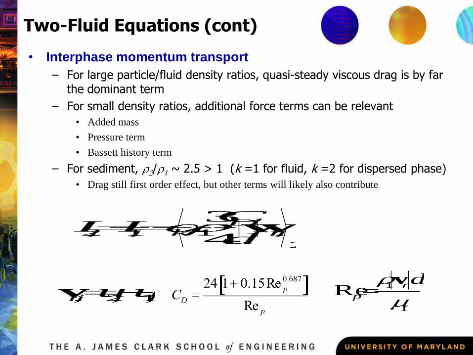
• Interphase momentum transport

– For large particle/fluid density ratios, quasi-steady viscous drag is by far the dominant term

– For small density ratios, additional force terms can be relevant

• Added mass

• Pressure term

• Bassett history term

– For sediment, / ~ 2.5 > 1 (k =1 for fluid, k =2 for dispersed phase)

• Drag still first order effect, but other terms will likely also contribute

2

,1,1,24

3irr

Dkii

d

CII vv

iiir uu ,1,2,v CD

24 1 0.15Re p

0.687

Re p 1

1Re

dr

p

v

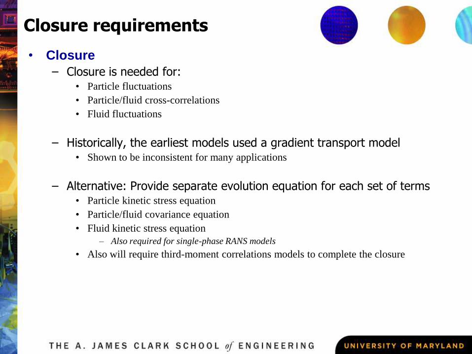
Closure requirements

• Closure

– Closure is needed for:• Particle fluctuations

• Particle/fluid cross-correlations

• Fluid fluctuations

– Historically, the earliest models used a gradient transport model• Shown to be inconsistent for many applications

– Alternative: Provide separate evolution equation for each set of terms• Particle kinetic stress equation

• Particle/fluid covariance equation

• Fluid kinetic stress equation

– Also required for single-phase RANS models

• Also will require third-moment correlations models to complete the closure

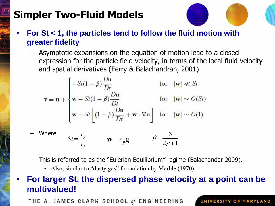
Simpler Two-Fluid Models

• For St < 1, the particles tend to follow the fluid motion with

greater fidelity

– Asymptotic expansions on the equation of motion lead to a closed expression for the particle field velocity, in terms of the local fluid velocity and spatial derivatives (Ferry & Balachandran, 2001)

– Where

– This is referred to as the “Eulerian Equilibrium” regime (Balachandar 2009).

• Also, similar to “dusty gas” formulation by Marble (1970)

• For larger St, the dispersed phase velocity at a point can be

multivalued!

Stp

f

w pg3

2 1

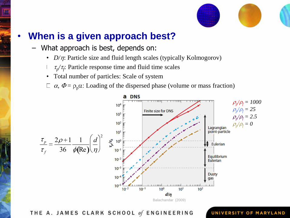
• When is a given approach best?– What approach is best, depends on:

• D/ : Particle size and fluid length scales (typically Kolmogorov)

p/ f: Particle response time and fluid time scales

• Total number of particles: Scale of system

, = p Loading of the dispersed phase (volume or mass fraction)

Balachandar (2009)

p

f

2 1

36

1

Re

d2

p/ f = 1000

p/ f = 25

p/ f = 2.5

p/ f = 0

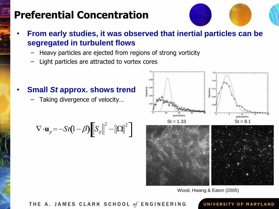
• From early studies, it was observed that inertial particles can be

segregated in turbulent flows

– Heavy particles are ejected from regions of strong vorticity

– Light particles are attracted to vortex cores

• Small St approx. shows trend

– Taking divergence of velocity…

Preferential Concentration

Wood, Hwang & Eaton (2005)

St = 1.33 St = 8.1

up St 1 Sij

2 2

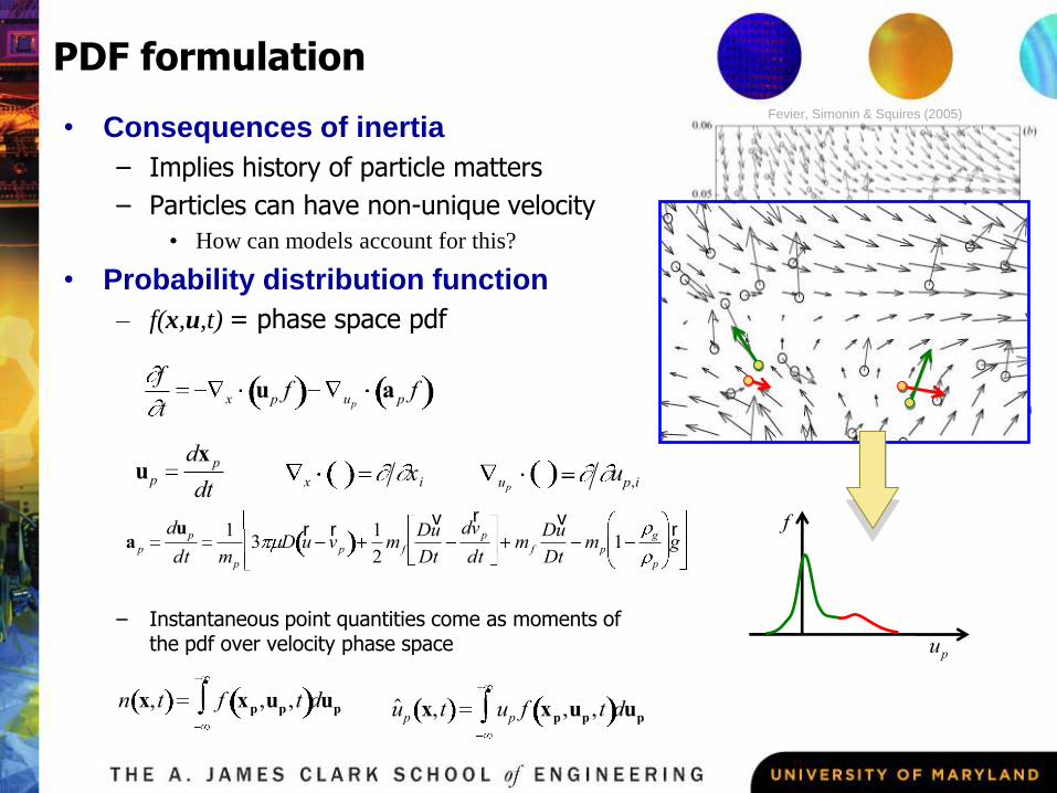
PDF formulation

• Consequences of inertia

– Implies history of particle matters

– Particles can have non-unique velocity

• How can models account for this?

• Probability distribution function

– f(x,u,t) = phase space pdf

– Instantaneous point quantities come as moments of the pdf over velocity phase space

n x,t f xp,up ,t dup

f

tx up f up

a p f

x xi upup,i

up

dx p

dt

a p

dup

dt

1

mp

3 Dr u

r v p

1

2m f

Dv u

Dt

dr v p

dtm f

Dv u

Dtmp 1

g

p

r g

Fevier, Simonin & Squires (2005)

ˆ u p x,t up f xp,up ,t dup

up

f

Examples

• Effect of particles on shear layer instability

• Particle-Fluid Coupling in sediment transport

• Case studies in interface tracking methods

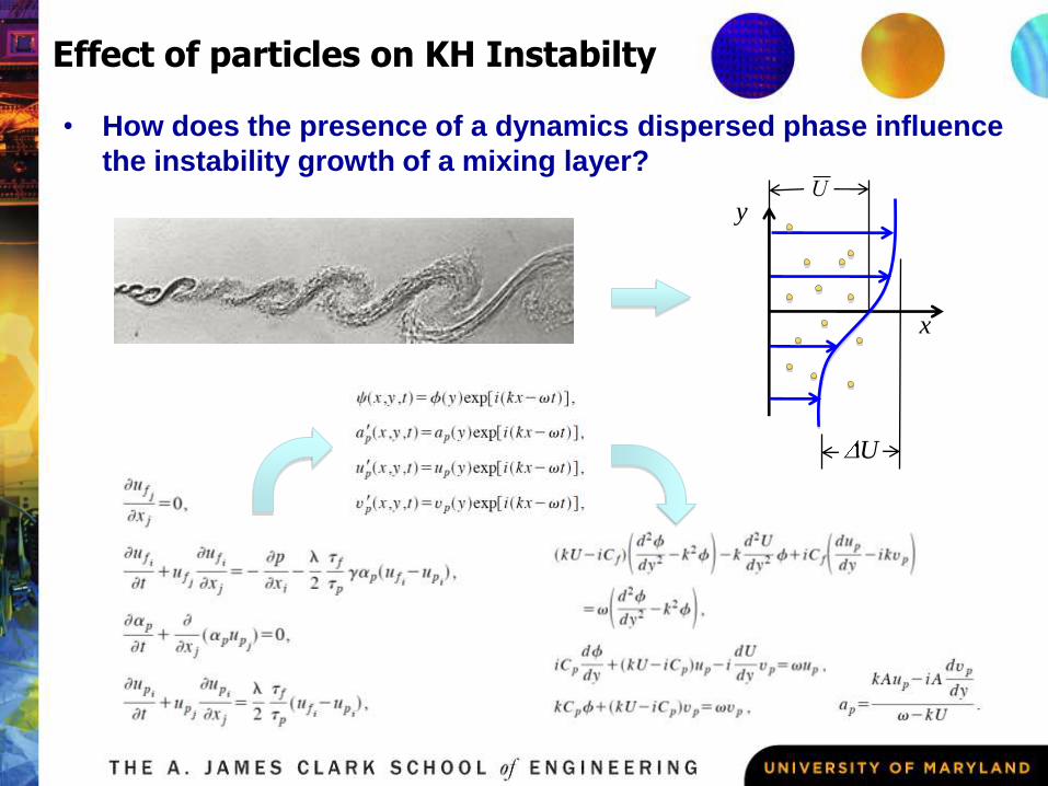
Effect of particles on KH Instabilty

• How does the presence of a dynamics dispersed phase influence

the instability growth of a mixing layer?

x

y

U

U

Results

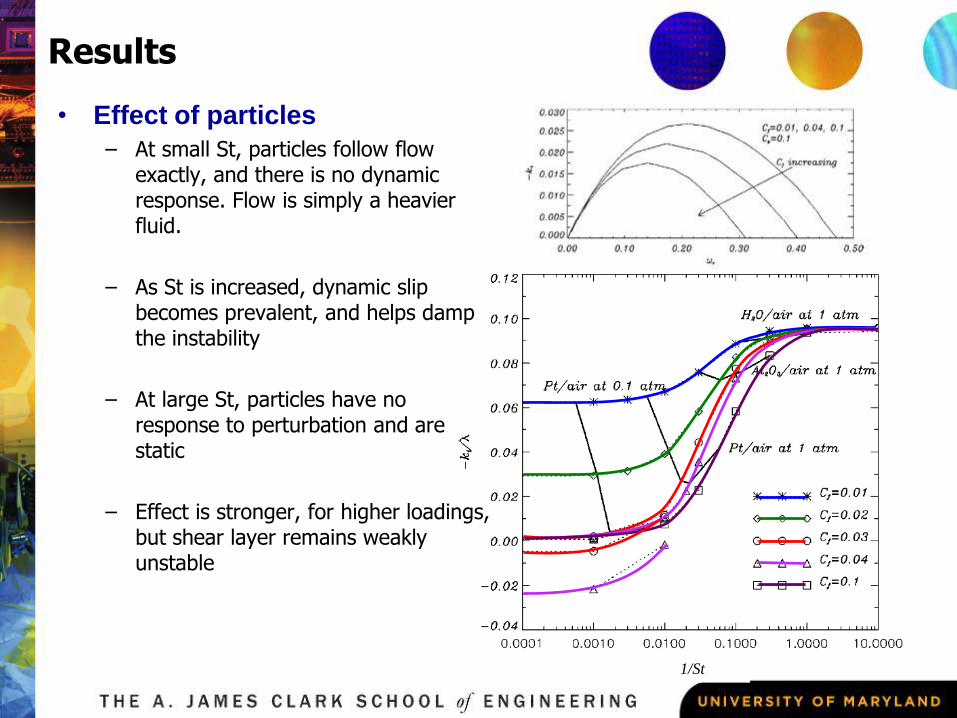
• Effect of particles

– At small St, particles follow flow exactly, and there is no dynamic response. Flow is simply a heavier fluid.

– As St is increased, dynamic slip becomes prevalent, and helps damp the instability

– At large St, particles have no response to perturbation and are static

– Effect is stronger, for higher loadings, but shear layer remains weakly unstable

1/St

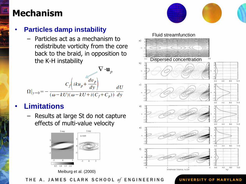
Mechanism

• Particles damp instability

– Particles act as a mechanism to redistribute vorticity from the core back to the braid, in opposition to the K-H instability

• Limitations

– Results at large St do not capture effects of multi-value velocity

Fluid streamfunction

Dispersed concentration

up

Meiburg et al. (2000)

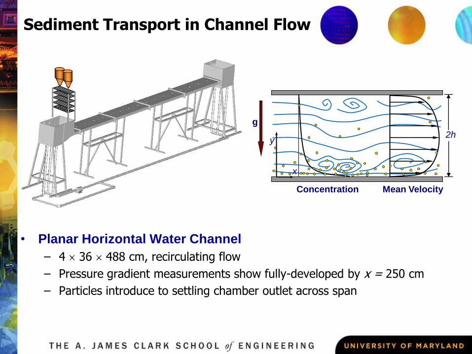
Sediment Transport in Channel Flow

• Planar Horizontal Water Channel

– 4 36 488 cm, recirculating flow

– Pressure gradient measurements show fully-developed by x = 250 cm

– Particles introduce to settling chamber outlet across span

Concentration Mean Velocity

g

x

y2h

• Both single-phase and two-phase experiments conducted

• Carrier Fluid Conditions

– Water, Q = 7.6 l/s

– Uc = 59 cm/s, u = 2.8 cm/s, Re = 570

– Flowrate kept the same for two-phase experiments

– Tracer particles: 10 m silver-coated, hollow glass spheres, SG = 1.4

• Dispersed Phase Conditions

– Glass beads: (specific gravity, SG = 2.5)

– Standard sieve size range: 180 < D < 212 m

– Settling velocity, vs = 2.2 to 2.6 cm/s

– Corrected Particle Response Time, = 4.5 ms

– St+ = p/+ ~ 4

– Bulk Mass Loading: dM/dt = 4 gm/s, Mp/Mf ~ 5 10-4

– Bulk Volume Fraction, = 2 10-4

Experimental Conditions

p

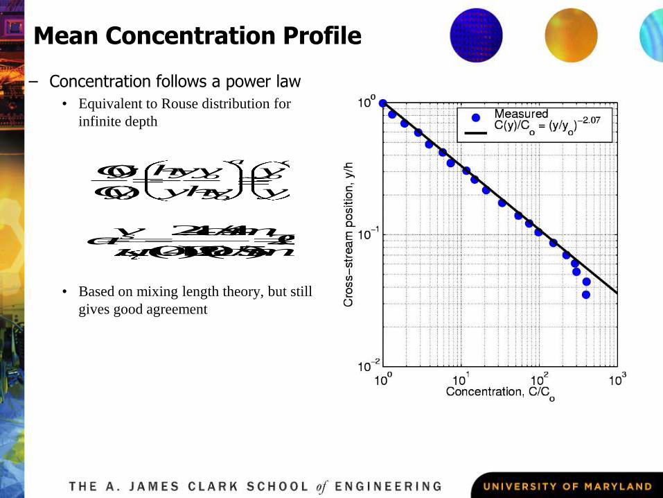
– Concentration follows a power law

• Equivalent to Rouse distribution for

infinite depth

• Based on mixing length theory, but still

gives good agreement

Mean Concentration Profile

a

o

a

o

o

o y

y

yh

y

y

yh

yC

yC

)(

)(

07.2)/95.2)(40.0(

/44.2

scm

scm

u

vas

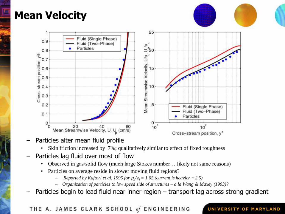
Mean Velocity

– Particles alter mean fluid profile• Skin friction increased by 7%; qualitatively similar to effect of fixed roughness

– Particles lag fluid over most of flow• Observed in gas/solid flow (much large Stokes number… likely not same reasons)

• Particles on average reside in slower moving fluid regions?

– Reported by Kaftori et al, 1995 for p/ f = 1.05 (current is heavier ~ 2.5)

– Organization of particles to low speed side of structures – a la Wang & Maxey (1993)?

– Particles begin to lead fluid near inner region – transport lag across strong gradient

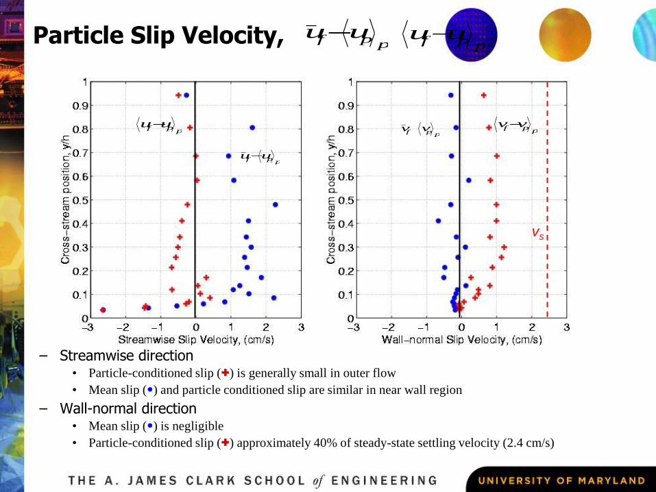
Particle Slip Velocity,

– Streamwise direction• Particle-conditioned slip (+) is generally small in outer flow

• Mean slip (•) and particle conditioned slip are similar in near wall region

– Wall-normal direction• Mean slip (•) is negligible

• Particle-conditioned slip (+) approximately 40% of steady-state settling velocity (2.4 cm/s)

ppf uuppf uu

ppf uu

ppf uuppf vv ppf vv

vs

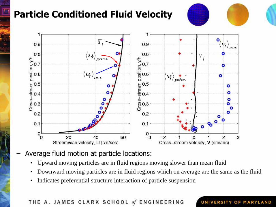
Particle Conditioned Fluid Velocity

– Average fluid motion at particle locations:

• Upward moving particles are in fluid regions moving slower than mean fluid

• Downward moving particles are in fluid regions which on average are the same as the fluid

• Indicates preferential structure interaction of particle suspension

downpfu ,

uppfu,

fu

fv

downpfv ,

uppfv,

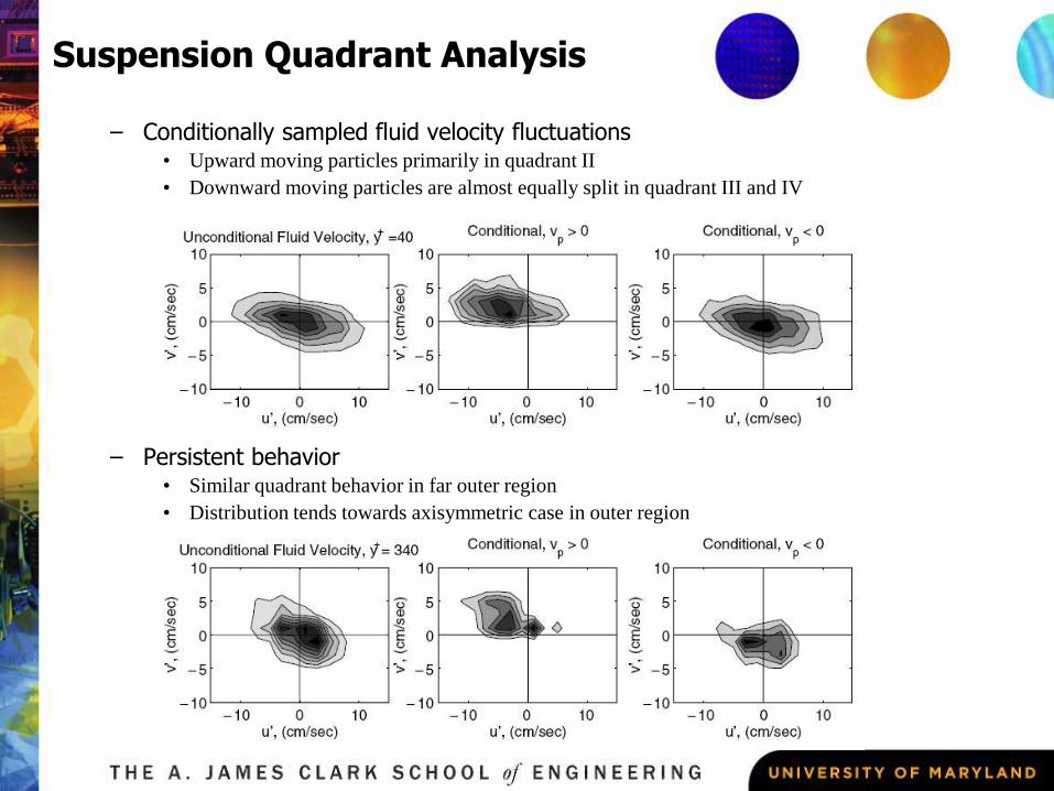
Suspension Quadrant Analysis

– Conditionally sampled fluid velocity fluctuations• Upward moving particles primarily in quadrant II

• Downward moving particles are almost equally split in quadrant III and IV

– Persistent behavior• Similar quadrant behavior in far outer region

• Distribution tends towards axisymmetric case in outer region

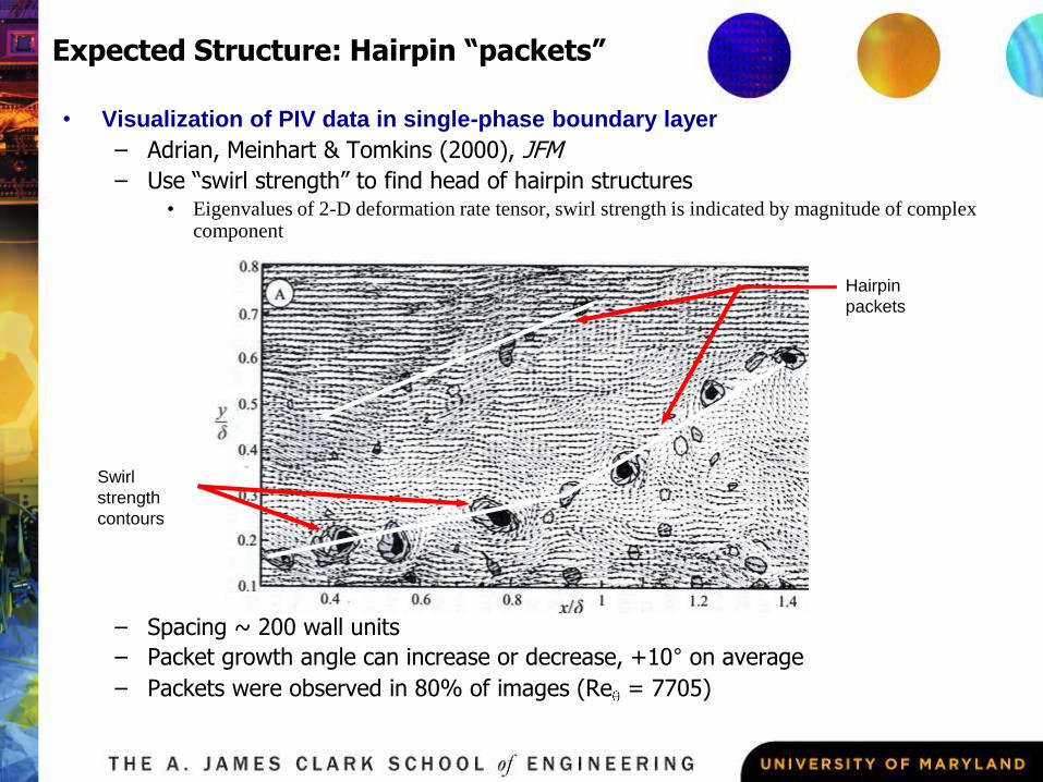
Expected Structure: Hairpin “packets”

• Visualization of PIV data in single-phase boundary layer

– Adrian, Meinhart & Tomkins (2000), JFM

– Use “swirl strength” to find head of hairpin structures • Eigenvalues of 2-D deformation rate tensor, swirl strength is indicated by magnitude of complex

component

– Spacing ~ 200 wall units

– Packet growth angle can increase or decrease, +10° on average

– Packets were observed in 80% of images (Re = 7705)

Swirl

strength

contours

Hairpin

packets

Event structures: Quadrant II hairpin

• Similar structures found

– Appropriate spacing

– Not as frequent• Re effects? (Re = 1183)

• Smaller field of view?

• Evidence suggests packets contribute to particle suspension

Q2 & Q4

contribution

s

Swirl

Strength

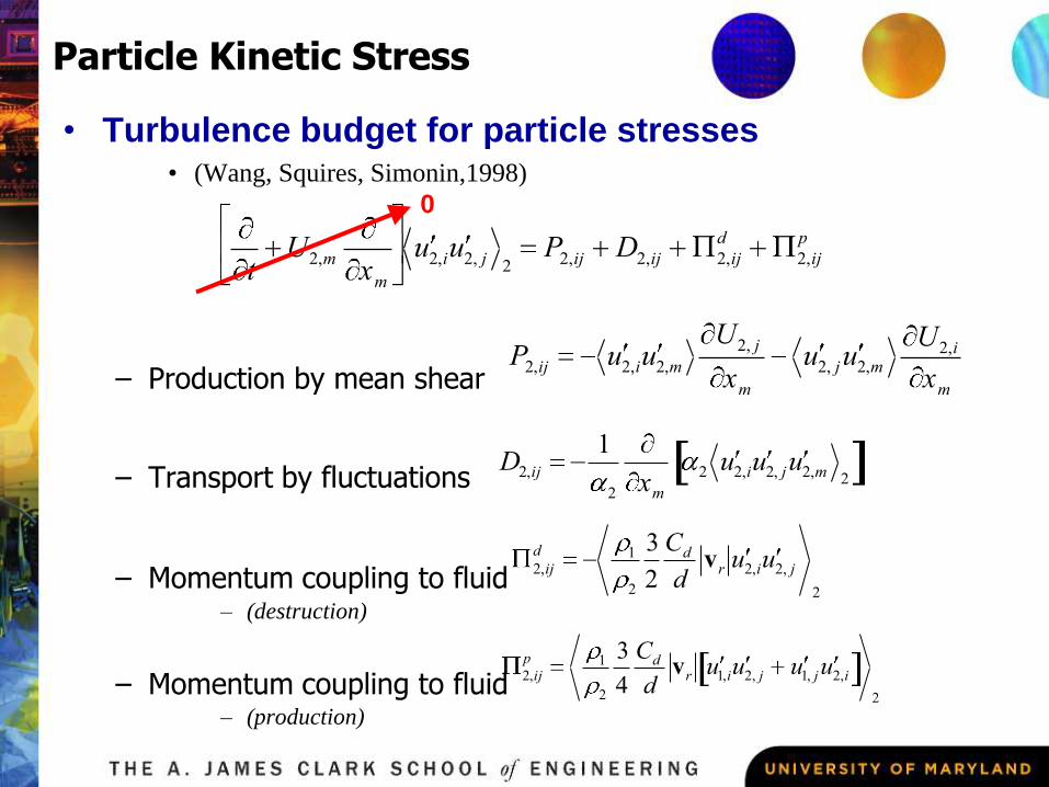
• Turbulence budget for particle stresses • (Wang, Squires, Simonin,1998)

– Production by mean shear

– Transport by fluctuations

– Momentum coupling to fluid – (destruction)

– Momentum coupling to fluid – (production)

Particle Kinetic Stress

tU2,m

xm

u 2,iu 2, j 2P2,ij D2,ij 2,ij

d

2,ij

p

P2,ij u 2,iu 2,m

U2, j

xm

u 2, ju 2,m

U2,i

xm

D2,ij

1

2 xm

2 u 2,iu 2, ju 2,m 2

2,ij

p 1

2

3

4

Cd

dvr u 1,iu 2, j u 1, ju 2,i

2

2,ij

d 1

2

3

2

Cd

dvr u 2,iu 2, j

2

0

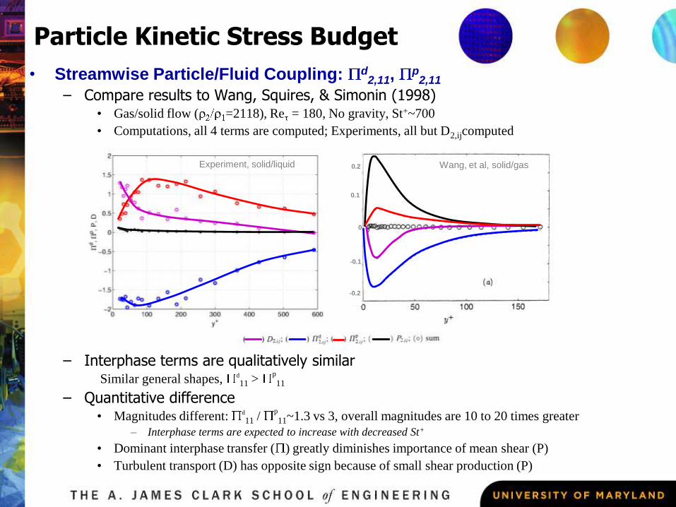
• Streamwise Particle/Fluid Coupling: d2,11,

p2,11

– Compare results to Wang, Squires, & Simonin (1998)• Gas/solid flow ( =2118), Re = 180, No gravity, St+~700

• Computations, all 4 terms are computed; Experiments, all but D2,ijcomputed

– Interphase terms are qualitatively similar Similar general shapes, d

11 > p

11

– Quantitative difference• Magnitudes different: d

11 / p

11~1.3 vs 3, overall magnitudes are 10 to 20 times greater

– Interphase terms are expected to increase with decreased St+

• Dominant interphase transfer ( ) greatly diminishes importance of mean shear (P)

• Turbulent transport (D) has opposite sign because of small shear production (P)

Particle Kinetic Stress Budget

0.2

0.1

0

-0.1

-0.2

Experiment, solid/liquid Wang, et al, solid/gas