Multiphase Pipelining - AEM · does not seem to be a literature on frictional heating in turbulent...

printed 11/30/00 1 DDJ/2000/proposals/DOE-multiphase/pipelineV3.doc

Proposal to the Department of Energy, Office of Basic Energy Sciences,

Division of Engineering

Multiphase Pipelining

Daniel D. Joseph

December 2000

I Research on fundamentals for multiphase pipelining ................................................... 1II Accomplishments of our previous DOE/DE-FG02-87ER 13798, 9/1/98--8/31/01...... 2III Lubricated transport of viscous oils. Friction factor efficiency ratio......................... 5IV Numerical simulation of laminar wavy core flow........................................................ 9V Numerical simulation of wavy core flow of oil in

turbulent water and turbulent gas-liquid flow with fouled pipe wall...................... 10VI Analysis of frictional heating in turbulent two-phase flow ....................................... 13VII Gas-liquid flow in pipelines....................................................................................... 14VIII Flow charts for gas-liquid flow. Multiple solutions. Transition to annular flow. 15IX Viscous potential flow (VPH) analysis of Kelvin-Helmholz instability in

rectangular conduits ................................................................................................. 17X Nonlinear effects. Bifurcation analysis of KH instability using

viscous potential flow. Multiple solutions. ............................................................... 23XI Rise velocity of long gas bubbles in pipes and conduits ............................................ 26XII Appendix A -Experimental facilities......................................................................... 33XIII Appendix B – Shear stress transport (SST) turbulence model............................... 34XIV References................................................................................................................. 37

I Research on fundamentals for multiphase pipeliningThis proposal focuses on a suite of fundamental problems of multiphase pipelining of

liquid-liquid and gas-liquid flows that arise in various branches of the oil industry. Wehave defined and developed methods of solution to the problems being proposed here. Allthese problems are academically viable and all are relevant to improvements in theproduction and transport of oil and gas.


Three broad categories of study will be undertaken.

(1) Analysis of the lubrication efficiency of core-annular flow of heavy oil inturbulent water. The organizing concept introduced here is the friction factor efficiencyratio, which is the ratio of the friction factor for core-annular flow to the friction factor ofturbulent flow of water alone at the same superficial velocity. This ratio is greater thanone due to extra dissipation that we believe is due to wave propagation on the oil coreand fouling. The problem of increased dissipation can be studied theoretically using aturbulence model we have adapted for this application. Using this model, various causesfor increased dissipation can be examined one at a time and compared with observedincreases of dissipation in laboratory experiments and Syncrude's commercial line. Avery large increase in temperature (over 50°C) due to frictional heating in pipelining ofbitumen froth was observed in 1" pipes, but not in the 36" commercial pipeline. Theproblem of frictional heating in turbulent core annular flow has not been studied; theredoes not seem to be a literature on frictional heating in turbulent pipelines even whenonly one phase is present; we intend to create such a literature.

(2) Studies of pipelining of gas-liquid flows. We will study stability and bifurcationof stratified flow using a new approach based on viscous potential flow. This transitionand pressure drop in annular gas-liquid flow will be studied using our turbulence modellooking again at the friction factor efficiency ratio, which here is the ratio of the frictionfactor of turbulent annular gas-liquid flow to turbulent gas flow when no liquid is on thewall. The huge experimental literature on annular flows can also be processed forunderstanding the sources of increased dissipation. Preliminary studies suggest that thedissipation increases sharply with the volume fraction of liquid on the wall.

(3) Experimental and numerical studies will be undertaken to explain anomalousproperties of Taylor bubbles of gas in water and heavy oils in vertical pipes and in theannulus between concentric vertical cylinders. The numerical studies will be carried outwith a fully 3D code based on level set methods that can be applied even tononaxisymmetric bubbles, which are always observed in annular pipes.

II Accomplishments of our previous DOE/DE-FG02-87ER13798, 9/1/98--8/31/01The projects proposed were focused on self-lubricated transport of bitumen froth.

This project was brought to us by Syncrude Canada at a time when they were evaluatingoptions for transporting bitumen froth from a newly opened Aurora mine 35 kilometers tothe upgrading facility at Lake Mildred. Bitumen froth is a stable water in oil emulsionwhich is created from the oil sands by a steam process in which most of the dirt andstones are removed. It is extremely important that the natural water left in this emulsion isa colloidal dispersion of clay particles that can be seen as the milk colored white fluid infigure 8. We found that the clay particles are crucial to the success of the technologysince they stick to the bitumen yet are hydrophilic, thus giving rise to a surfactant actionthat acts to keep the clay-covered bitumen from sticking to itself. After the water


coalesces into a lubricating film under shear, the oil on the wall is protected from thebuildup of fouling by the clay covering.

Very interesting fundamental problems came out of our DOE/Syncrude studies. Wediscovered a scale up law in which the friction factor vs. Reynolds number follows theBlasius turbulence relation in which the pressure gradient is proportional to the ratio ofthe 7/4th power of the velocity to the 5/4th power of the pipe radius at a cost of ten to 20times greater than water alone. These results were shown to hold 1”, 2” and 24” pipes inthe paper by Joseph, Bai, Mata, Grant and Sury, “Self-lubricated transport of bitumenfroth”, J. Fluid Mech. 386, pp 127-149 1999. Grant and Sury are from Syncrude.Sanders at Syncrude research in Edmonton confirmed the scale up law; together wedeveloped a froth rheometer to determine critical stress for self-lubrication and we foundthat cement lined pipes promote self-lubrication of bitumen froth because the clay in thenatural water promotes a strong wetting of cement by colloidal clay.

The Blasius scale up seems to be universal for lubricated flows in which thelubricating water layer is turbulent. The increased friction is apparently due to waves.The source of the increased friction is a topic of research because unlike roughness,which increases the exponent from 7/4 toward 2, the increase of friction in lubricatedflows does not change the exponent.

Based on our joint works withSyncrude people, Syncrude’s manage-ment authorized a 76 million dollarinvestment for the construction of a36” pipeline to run 35 kilometers fromthe Aurora mine to the upgradingfacility at Lake Mildred. Theengineering of this pipeline followsour scale up, since no tests were donein such a large pipeline. This line wasput into operation in August of 2000;it is a total success and transports frothat a cost 6 times more than wateralone, better than expected.

In their press release of August 17,2000 titled, "Syncrude's AuroraMine Heralds New Era of EnergyProduction for Canada, New tech-nology lowers cost and improves en-vironmental performance," they cointhe words "natural froth lubricity":


Long distance pipelining of bitumen froth is enabled by Natural Froth Lubricity. Thistechnology uses the water that is naturally evident in the froth to form a lubricating'sleeve,' thus allowing the froth to travel via pipeline without adding a diluent such asnaphtha.

A letter of recognition of the importance of our contribution to the Aurora projectappears above.

The idea of a lubricated gas-liquid flow was proposed by Bannwart and Joseph 1996.We are speaking of annular gas-liquid flow in which the liquid covers the pipe wall. Weproposed to think of this flow as lubricated; though the molecular viscosity of the gas ismuch lower than the eddy viscosity of the turbulent gas is larger. This theory worksextremely well for water, both in horizontal and vertical pipes but it is not in such goodagreement with data from other liquids. We believe that the basic and new idea that thestabilization of annular flow is due to the increased flow resistance of the turbulent gas issound and we are going to see if we can come up with an acceptable modification of ourtheory which is compatible with all the data.

Our studies of the lubricated transport of slurries have been carried out using directnumerical simulation. We have become world leaders in this kind of work and will beable to exploit these new opportunities in the next years. Our main work in this arenaduring the last year focused on surgical analysis of the inertial, normal stress, shearthinnings and combined effects on the migration of neutrally buoyant particles inPoiseuille flow.

We were recently funded by Exxon-Mobil to do small studies of the lubricationoptions for a new pipeline they are going to build in Africa.

I have listed the papers that are most relevant to our ongoing work as described herebelow:

Lubricated Transport

1. A. Bannwart and D.D. Joseph, 1996. “Stability of annular flow and slugging” Int.J. of Multiphase Flow 22 (6), 1247-1254.

2. D.D. Joseph, 1997. “Steep wave fronts on extrudates of polymer melts andsolutions: Lubrication layers and boundary lubrication”, J. Non-Newtonian FluidMech., 70, 187-203.

3. G. Nunez, H. Rivas, D.D. Joseph, Oct. 26, 1998. Drive to produce heavy crudeprompts a variety of transportation methods. Oil and Gas Journal, 59-68

4. D.D. Joseph and R. Bai, 1999. Interfacial Shapes in the Steady Flow of a HighlyViscous Dispersed Phase. Fluid Dynamics at Interfaces Ed. Wei Shyy, CambridgeUniversity Press.

5. D.D. Joseph, R. Bai, C. Mata, K. Surry and C. Grant, 1999. Self LubricatedTransport of Bitumen Froth. J. of Fluid Mech., 381, 127-149


6. R. Bai and D.D. Joseph, 1999. Steady flow and interfacial shapes of a highlyviscous dispersed phase. Int. J. Multiphase Flow, 26 (8)

7. P. Huang and D.D. Joseph, 2000. “Effects of shear thinning on migration ofneutrally buoyant particles in pressure driven flow of Newtonian and Viscoelasticfluids”, J. Non-Newtonian Fluid Mech., 90, 159-185.

8. C. Mata, M.S. Chirinos, M.E. Gurfinkel, G.A. Núñez and D.D. Joseph, 2001.“Pipeline transport of highly concentrated oil in water emulsions.” SPE paper, toappear.

9. S. Sanders, R. Bai and D.D. Joseph. “Self lubricated transport of bitumen froth;effect of bulk property change and internal pipe coatings.” Under preparation.

10. T.A. Smieja, D.D. Joseph, G. Beavers, 2000. “Flow charts and lubricatedtransport of foams,” Int. J. Multiphase Flow, submitted.

Honors and awards since 1997 (grant start year):

• Illinois Institute of Technology Professional Achievement Award, 1998• Kovasznay Lecturer, University of Houston, Mechanical Engineering, April 1999• University of Chicago, Professional Achievement Award, May 1999• Fluid Dynamics Prize of the American Physical Society, November, 1999Patents obtained:• US Patent 5,988,198. Process for pumping bitumen froth through a pipeline. O.

Nieman, K. Sury, D.D. Joseph, R. Bai and C. Grant.

III Lubricated transport of viscous oils. Friction factorefficiency ratio.The usual notion of lubrication of a solid carries over to the lubrication of a very

viscous liquid by a less viscous one. Nature's gift is that the less viscous liquid migratesinto regions where the shear is greatest, minimizing dissipation, lubricating the flow. Inmany of the practical cases, and all those considered here, water lubricates oil. In pipeflows the region of high shear is at the pipe wall, which is where the water migrates.Lubricated flow is hydrodynamically stable, if the oil doesn't stick to the wall and thenstick to itself building up fouling, water will go to the wall stably. In the best cases thepressure gradients used to drive water-lubricated flows can be even less than thoseneeded to transport water alone. This can lead to pressure gradient reductions of the orderof the viscosity ratio, which can be factors of the order 105.

There are three ways to create a water lubrication of oils: (1) core annular flows, inwhich oil and water are pumped simultaneously, (2) self-lubricated flow of water in oilemulsions, in which the droplets of water are in a thermodynamically stable range, say30%-40% and form a lubricating layer suddenly, at a critical rate of shear, (3) lubricatedflow of concentrated oil in water emulsions, in which lubrication is achieved by


migration of oil droplets away from the wall wringing water out of the core of theemulsion.

All three modes of lubrication have been used in pipelining, depending on localconditions.

The science and technology of core-annular flows, in which oil and water are pumpedsimultaneously, has a long history since the early 1900's, which is reviewed by Joseph &Renardy 199211 and Joseph, Bai, Chen and Renardy 199712.

Core-annular flows can be established only in oils of viscosity greater than 500 cp(rule of thumb with some theoretical backup.)

The main threats to core annular flow are

(i) Stratification. When the density difference of oil-and water is large, or

when the flow is very slow. It takes inertia associated with waves to levitate

the core away from the wall.

(ii) Fouling. There are two parts to fouling. The oil may stick to the wall; this is

an energy effect and it depends on the oil and pipe wall interaction

measured by contact angles. If the wall is oleophobic, it won't foul and the

hydrodynamics will put the water on the wall.

More important than fouling is buildup of fouling. Here we know that the wall foulsand we ask if the oil wants to stick to itself; if it does, we will get a buildup of fouling andfailure. This depends on the oil and what's in the water. With the right choice ofsurfactants we might prevent an oil from sticking to itself.

Self-lubricated flow of water in oil emulsions does not require separate pumping ofoil and water. Little water droplets of modest volume fraction, say 20% or 30%, aredispersed throughout the oil. The viscosity of this dispersion is even larger than the oilalone. To get lubrication you need to break the emulsion by shearing at the wall (seeKruka 1977)13. This implies that there is a critical speed at which the shear becomes largeenough to break the emulsion.

We plotted up the data in Kruka's patent; it is displayed as figure 1.


Figure 1. Kruka's data is for 90/10 o/wemulsion using Midway Sunset crude in a1/2" pipeline. We predict 5 m/sec arerequired to break 70/30 o/w emulsion.

0.1

1

10

10 100 1000

Data from Kruka

Fitted curvepredicted Exxon value (5 m/s)

Syncrude data

Sp

eed

(m

/s)

Viscosity (poise)

There is almost no literature on self-lubrication of water in oil emulsions. BesidesKruka's patent, there are reports of self-lubrication of Syncrude's bitumen froth, which isan emerging technology. Syncrude's case is special because the clay in the natural waterkeeps the oil from sticking to itself; we call this powdering the dough. The patent for thispumping process is described by Neiman et al 199914.

Syncrude Canada Ltd. contacted us in 1994 to study self-lubrication of bitumen froth.They were particularly interested in fouling as a possible show stopper for self-lubricatedpipelining which in-house 1985 studies of O. Nieman15 suggested might be a viableoption for pipelining froth from the mine. Our studies showed that though the pipelinesfouled initially, no buildup of fouling would occur. Results of our studies of start andrestart of a stopped line were similarly successful. Motivated by the success of theMinnesota studies, Syncrude built a 24"× 1km pilot loop in Fort McMurray. The resultsof these tests confirmed the Minnesota studies and they provided a database from whichwe determined a powerful scale-up result described in the abstract16 partly reproducedhere:

"Bitumen froth is produced from the oil sands of Athabasca using the Clark’s Hot WaterExtraction process. When transported in a pipeline, water present in the froth is releasedin regions of high shear; namely, at the pipe wall. This results in a lubricating layer ofwater that allows bitumen froth pumping at greatly reduced pressures and hence thepotential for savings in pumping energy consumption. Experiments establishing thefeatures of this self-lubrication phenomenon were carried out in a 1" diameter pipeloop atthe University of Minnesota, and in a 24" (0.6m) diameter pilot pipeline at Syncrude,Canada. The pressure gradient of lubricated flows in 1"(25mm), 2"(50mm) and24"(0.6m) pipes diameters closely follow the empirical law of Blasius for turbulent pipeflow; the pressure gradient is proportional to the ratio of the 7/4th power of the velocityto the 4/5th power of the pipe diameter, but the constant of proportionality is about 10 to20 times larger than that for water alone… "

The Blasius expression for a single fluid with viscosity µ, density ρ, velocity U,pressure gradient β= = ∆P/L in a pipe of radius R can be written as


4/5

4/74/1

9

3

2316.0

RU

= µρψβ (1)

where ψ is the friction factor efficiency ratio, the ratio of the friction factor in two-phaseflow to the friction factor for water and gas alone; ψ== 1 is for the flow of a single fluid.It is well known and at first surprising that in ideal lubrication in which the core is veryviscous, without waves, and the flow of water is laminar, then for a given volume flux thepressure gradient can be smaller than for water. Equation (1) does not apply to laminarflow but an equivalent formula, linear in the mean velocity, would yield a high efficiencywith ψ < 1. The presence of waves and fouling increase ψ. When dealing with turbulentannular flow, even with turbulent gas-liquid annular flow, it is important to know thevalue of ψ and how ψ depends on parameters.

Figure 2. Curve fits parallel to the Blasius correlation for turbulent pipe flow (water alone), fortemperature range 41-47°C. 14

For Syncrude froth in the pilot pipelines mentioned in the abstract ψ is between 10and 20, and depends strongly on temperature (figure 2). In the 36" commercial line thatwas designed using the relation (1), the value of ψ is about 6, indicating more efficientlubrication.

The various components of our study of turbulent annular flow can ultimately beexpressed in terms of factors that determine the two-phase flow function ψ. This functiontakes values rather larger than 1 due to fouling of the walls. When the oil on the wall isprotected from the buildup of fouling, as in the case of froth covered by clay, waves onthe pipe are also driven by turbulent water at a cost in the pressure gradient reflected inthe multiplicative factor ψ >1. This increased friction is not like a rough pipe in which the


exponent n (7/4 ≤ n ≤ 2) of Un is increased over 7/4 rather than in a multiplicative factorlike ψ.

IV Numerical simulation of laminar wavy core flowAnalysis of problems of levitation, transitions between flow types, pressure gradients

and hold-up ratios have been carried out by direct numerical simulation. Bai, Kelkar andJoseph17 1996 did a direct simulation of steady axisymmetric, axially periodic CAF,assuming that the core viscosity was so large that secondary motions could be neglectedin the core. They found that wave shapes with steep fronts like those shown in Figure 3always arise from the simulation, see figure 4. The wave front steepens as the speedincreases. The wave shapes are in agreement with the shapes of bamboo waves in up-flows studied by Bai, Chen and Joseph18 1992. Better agreements were obtained by theperturbation analysis for steady flow of a highly but not infinitely viscous core of Bai andJoseph6 1999 in which account is taken of flow motions in the core. Li and Renardy19

1999 were the first to solve the initial value problem for computed bamboo waves invertical core annular laminar flow using a volume of fluid method. Their results are inexcellent agreement with experiments of Bai et al 1992. They found an unsteady solutionin which the velocity and pressure in the water change with time but the interfacialshapes are steady.

g

Water

Water

Oil

Figure 3. The high pressure at the front of the wave crest steepens the interface and the lowpressure at the back makes the interface less steep. The pressure distribution in the troughdrives an eddy in each trough.


Figure 4. Streamlines and secondary motion for (a) rigid core and (b) perturbation theorywhen [η,h,R,J] = [0.8, 1.4, 600, 13 × 104].20

V Numerical simulation of wavy core flow of oil in turbulentwater and turbulent gas-liquid flow with fouled pipe wallIn most pilot and test loops, and all commercial lines, the water in the annulus

surrounding the oil core is turbulent and the flow in the viscous core is laminar. If the oilviscosity is very large, as is true of heavy oils and bitumen froth, secondary flows and thepressure gradients that produce them may be ignored.

Ko, Choi, Bai and Joseph21 2000 have developed a numerical method to predictwaves on the core of viscous oil in turbulent water. The numerical code is based on the k-ω (shear stress transport) method proposed by Menter22 1994. There are no adjustableparameters in this code. Computed results using this code are in agreement withexperiments. A few of these results are mentioned below (see table 1 and figure 7) andmore can be found in the paper posted on our web site, http://www.aem.umn.edu /Solid-Liquid_Flows/.

We are proposing to use our code to study the efficiency of lubrication (thecoefficient ψ in the Blasius expression (1)) in core flow of viscous oil in an annulus ofturbulent water next to a fouled pipe wall, and in a turbulent gas flow in a pipe whosewalls are covered by a liquid (annular gas-liquid flow).


We used Menter's shear stress transport k-ω model to solve the turbulent kineticenergy and dissipation rate equations (see Appendix B), and a four step fractional splitmethod to solve the Navier-Stokes equations. A streamline upwind Petrov-Galerkinmethod is adopted for the convection dominated flow. Menter's model utilizes theoriginal k-ω model of Wilcox in the inner region of the boundary layer and switches tothe standard k-ε model in the outer region of the boundary layer.

The turbulent code was validated for the case of developing Poiseuille flow in theflow of a single fluid in a pipe at Reynolds numbers from 200 to 40,000. The length ofthe computational domain is sufficient to get a fully developed profile for velocity,pressure and kinetic energy. The numerical simulation reproduces the laminar frictionfactor λ = 64/Re and turbulent friction factor λ = 0.316/Re1/4 with high accuracy (figure5) and the velocity profile in developed flow is close to the values computed by directnumerical simulation (figure 6).

0.01

0.1

1

100 1000 10000 100000Re

l

Numerical Result

l = 64/Re

l = 0.316/Re0.25

Figure 5. The friction factor vs. Reynoldsnumber in the fully developed pipe flow.

0

0.5

1

0 0.5 1

Direct numerical simulationOur calculationWilcox's k-w Model

Y/ R

U / U max

Figure 6. The velocity profile of the turbulentpipe flow at Re = 40,000.

0.0

0.0

0.1

1.0

10.0

1 10 100 1000U1.75/RO

1.25

Diameter = 1.27 cm Diameter = 2.54 cm Diameter = 5.08 cm Blasius correlation

Figure 7. Pressure gradient vs. Blasius parameter U1.75/R1.25 for wavy core annular flow.


Ko et al 2000 applied the turbulence code to the computation of waves and frictionfactor on a very viscous core in which the core moves forward with a uniform motion(relative motion in the core is suppressed) but the core deforms under normal stressesfrom turbulent water. This kind of approximation was introduced by Bai, Kelkar andJoseph15 1996 for laminar flow. The effects of turbulence may be suppressed in themodel by putting k = 0; in this case we have the "laminar" flow equations of Bai et al1996. Turbulence has a very strong effect as is seen in table 1, where experiments of Bai,Chen and Joseph 1992 are compared with results from the laminar and turbulentcalculations; the results computed with the turbulent code are much closer toexperiments, and the error decreases as the Reynolds number increases.

The Blasius friction factor correlation (1) was also computed using the turbulentcode. The code gives rise to a perfect agreement with the Blasius correlation with respectto the dependence on the velocity U 7/4 and radius RO

5/4. The two-phase flow factorψ = 3.17/3.16 for this calculation is essentially ψ== 1. It can be said that wavy core flowof an infinitely viscous core in turbulent water can be transported as cheaply as wateralone.

Reynolds Number 4000.2 4684.6 5333.6 5811.5 8000.4

Experiments 1.35786 1.23102 1.07574 1.02346 0.82907Laminar Code 1.91 1.83 1.76 1.72 1.6

DimensionlessWavelength(L*) Turbulent Code 1.55 1.34 1.2 1.11 0.9

Laminar Code 28.9078 32.7311 38.8784 40.4963 48.1828Error (%)Turbulent Code 12.3961 8.13281 10.355 7.79613 7.88061

Table 1. The comparison of measured and computed values of wavelength at h = 1.4 andη = 0.826.

To explain the increase in the frictional resistance (ψ = 10 or 20) in the self-lubricatedflow of bitumen froth evident in figure 2 we need to consider the dissipation due to thepropagation of waves in the oil. Waves do not propagate on the infinitely viscous case;this is probably why ψ== 3.17/3.16 for this case. In the next turbulence calculation wewill relax the assumption that the core is infinitely viscous (as we did in the laminar casein figure 4) and then calculate ψ. The large increase in ψ=seen in figure 2 is very likelydue to fouling waves develop on the fouled walls of the pipe; these are the "tiger waves"shown in figure 9. The same kind of waves occur in annular flows of turbulent gasdriving liquid waves, shown in figure 10. Ultimately we are proposing to do turbulencecalculations for the situations in figures 9 and 10.

Figure 8. (Joseph, Bai, Mata, Sury, Grant 1999.) Tiger waves of bitumen froth in water with

colloidal clay.


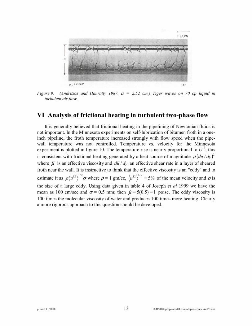
Figure 9. (Andritsos and Hanratty 1987, D = 2.52 cm.) Tiger waves on 70 cp liquid inturbulent air flow.

VI Analysis of frictional heating in turbulent two-phase flowIt is generally believed that frictional heating in the pipelining of Newtonian fluids is

not important. In the Minnesota experiments on self-lubrication of bitumen froth in a one-inch pipeline, the froth temperature increased strongly with flow speed when the pipe-wall temperature was not controlled. Temperature vs. velocity for the Minnesotaexperiment is plotted in figure 10. The temperature rise is nearly proportional to U 2; thisis consistent with frictional heating generated by a heat source of magnitude ( )2/ dyudµwhere µ is an effective viscosity and dyud / an effective shear rate in a layer of shearedfroth near the wall. It is instructive to think that the effective viscosity is an "eddy" and to

estimate it as σρ2/112u where ρ = 1 gm/cc, %5

2/112 =u of the mean velocity and σ isthe size of a large eddy. Using data given in table 4 of Joseph et al 1999 we have themean as 100 cm/sec and σ = 0.5 mm; then 1)5.0(5ˆ ==µ poise. The eddy viscosity is100 times the molecular viscosity of water and produces 100 times more heating. Clearlya more rigorous approach to this question should be developed.


40

45

50

55

60

65

0 2 4 6 8 10

Tem

pera

ture

(C

)

U2

Figure 10. Temperature vs. the square of the flow speed in a 25mm diameter pipe. Thetemperature of the room was 26°C and the froth temperature was not controlled; the increasein temperature is due to frictional heating.

Data from Syncrude's 36" commercial pipeline does not give evidence of frictionalheating. This suggests that frictional heating is a strong function of pipe diameter and thatscaling laws are far from evident.

We have not found a literature on frictional heating of multiphase pipelining. We areproposing to carry out a mathematical analysis of frictional heating of core annular flowboth in laminar and turbulent flow. One goal is the development of k-ω model for thetemperature generated by heat dissipation in turbulent water. We would seek to predictdata obtained in our one-inch pipeline and in Syncrude's 36" commercial pipeline.

The development of a working theory of frictional heating in turbulent multiphasepipelining is a challenging modeling problem whose solution could have practicalapplications.

VII Gas-liquid flow in pipelinesWe are going to bring two new methods to the analysis of gas-liquid flows in

pipelines. The simulation method we plan to use to use to analyze turbulent annular gas-liquid flows (figure 10) has already been described. The second new method makes useof a theory of viscous and viscoelastic potential flow that is discussed in section IX. Thistheory will be applied to the study of stability and bifurcation of stratified flow inrectangular, circular, horizontal, tilted and vertical pipelines. The third method is anapplication of level set methods to several variants of the Taylor bubble. Unlike the othertwo methods, the level set method is not our invention; we are using the method to


explain anomalous results like the independence of the rise velocity on bubble and theenhancement of the rise velocity with wetted area of inserted rods and strips.

We plan collaborative studies of gas-heavy oil flows with Intevep S.A., which is theresearch division of PDVSA, the Venezuelan national oil company. I have worked withthis company for many years over a very wide range of projects. I have advised threeVenezuelan students from INTEVEP to a PhD and one to a Masters degree. At present, Ihave one Masters degree student and two PhD students from Intevep. The companysupports all these students; it costs them $250,000 to educate a PhD student. The qualityof these students is excellent since only the best are selected for such a scholarship.

Besides working with my students on academically viable projects of interest toIntevep and oil companies, generally I do research with people from the company, at thecompany for weeks three times a year and remotely at other times. Three or four archivalpapers authored jointly with Venezuelans have appeared year after year.

For this project I propose to work on gas liquid pipeline flows with a group of about 8persons at the company. We are going to focus on flow transitions and pressure dropformulas in cases of transport of hydrocarbons, which we have not yet a well developedunderstanding. New problems and approaches will be described in section III.

We have excellent experimental facilities to study gas liquid flows at Intevep that aredescribed in appendix 2. These facilities allow me to construct real tests of our theoreticalideas.

VIII Flow charts for gas-liquid flow. Multiple solutions.Transition to annular flow.Multiphase flow through pipes and annular ducts is an important technical subject in

the oil industry. Detailed knowledge of this kind of flow is fundamental for the oilproduction system's proper design. Multiphase flow systems are highly complex andmany aspects of its behavior are not well understood today. This lack of knowledge isespecially critical in the case of heavy/extra-heavy oils. In order to design the facilities(selection of pipes, pumps, motors, etc.) traditional correlations of pressure gradient areused. These correlations were developed using fluids with viscosities ranging from 1 to 5cP. Nevertheless, even for these low viscosity liquids, errors in pressure gradientcalculations can be between 20% 23 and 30% 24. These errors will be greater in the case ofextra-heavy oils that can have up to 3000 cp.

The study of gas-heavy oil flow is best done as an emphasis in a general study of gas-liquid flow in which flow regime transitions, like the transition from stratified to slugflow are targets.

The most common correlation used to calculate the conditions for the transition fromone flow regime to another is the Mandhane plot25 shown in figure 11.


Lin and Hanratty 198726 note that "…the general consensus is that this plot is mostreliable for air and water flowing in a small diameter pipe." They get a quite differentflow chart even for air and water, when the pipe diameter is larger as shown in figure 12.

Figure 11. (After Taitel & Dukler 1976).Comparison of theory and experiment. Water-air, 25°C, 1 atm, 2.5 cm. diameter, horizontal.

theory; Mandhane et al, 1974.Regime descriptions as in Mandhane.

Figure 12. (After Lin & Hanratty, 1987.)Flow regime map for air and waterflowing in horizontal 2.54cm and 9.53cmpipes.

The Mandhane charts cannot well describe the flow regimes that can arise in allcircumstances. The coordinates of the charts are superficial velocities, dimensionalquantities that do not reflect any consequence of similarity, Reynolds numbers, Webernumbers etc. Mandhane charts lack generality since each sheet requires specification of aset of relevant parameters like fluid viscosity, surface tension, pressure level and gasdensity, turbulence intensity data, pipe radius, gas fraction, etc.

Mandhane charts assume that flow regimes are unique and do not acknowledge thefact that nonlinear system allow multiple solutions; for example, Wallis and Dobson27

1973 have shown that apparently stable slug flow can be initiated by large disturbances inthe region where stratified flow is stable (see their section titled "Premature slugging").Slugs are always formed in the 2" Intevep flow loop in gas-oil (µ = 400 cp) flows at eventhe smallest velocities that can be achieved in the system. These slugs are separatedregions of apparently stable stratified flow with a perfectly flat free surface. The length ofstable stratified flow between slugs can be nearly the length of the flow loop. This mayalso be interpreted as "premature" slugging though it is more appropriate to describe it asa multiple solution; slug flow and stratified flow exist at one and the same point on theflow chart.


From the practical point of view the existence of multiple solutions point to thedesirability of a careful analysis of domains of attraction of stable solutions. Theappearance of slugs in a region of stable stratified flow points to a careful analysis of thedisturbance level at the inlet where large waves may be created. At the end of the paperon waves Crowley, Wallis and Barry28 1992 write that

When a new slug forms it requires additional pressure drop to accelerate it. This feedsback to the inlet by acoustic waves in the gas (which can travel upstream) and changesthe conditions there. This new "disturbance" eventually grows to form a slug and thecycle repeats. The method of characteristics can represent this cycle, but assumptions (ora separate mechanistic analysis) are needed about this inlet behavior.

It is at present not possible to predict the transition of one flow type to another. Thedependence of the empirical charting of flows is also incomplete; there is only sparse dataon the dependence of flow type on pipe radius, liquid viscosity, pressure level,atomization level, turbulent intensity. Pressure gradients vs. volume flux, holdup ofphases and other process control data are not predictable from first principles or fromempirical flow charting.

We propose to study the transition of stratified flow to wavy flow and the transition toannular flow in hydrocarbon systems with viscosities greater than 100 cp. We are goingto analyze the effect of turbulence on the flow charts in general and for the targetedsystems; we will use our k-ω model and experimental data to determine the increases inthe pressure drop in annular flow due to liquid on the wall and atomization over thepressure drop for turbulent gas flow for dry gas in a clean pipe. This increase will beexpressed in terms of the friction factor efficiency factor ψ defined in equation (1).

We are also looking at y by processing the huge database in the literature. Our studieshave already suggested that increases in friction correlate with the amount of liquid onthe wall, with liquid holdup. Wave propagation in a deep liquid layer might increasefriction. Unfortunately, holdup data is not usually given in published data.

IX Viscous potential flow (VPH) analysisof Kelvin-Helmholz instability in rectangular conduitsIt is well known that the Navier-Stokes equations are satisfied by potential flow; the

viscous term is identically zero when the vorticity is zero but the viscous stresses are notzero (Joseph and Liao29 1994). It is not possible to satisfy the no-slip condition at a solidboundary or the continuity of the tangential component of velocity and shear stress at afluid-fluid boundary when the velocity is given by a potential. The viscous stresses enterinto the viscous potential flow analysis of free surface problems through the normal stressbalance at the interface. Viscous potential flow analysis gives good approximations tofully viscous flows in cases where the shears from the gas flow are negligible; theRayleigh-Plesset bubble is a potential flow which satisfies the Navier-Stokes equationsand all the interface conditions. Joseph, Belanger and Beavers30 1999 constructed a


viscous potential flow analysis of the Rayleigh-Taylor instability that can scarcely bedistinguished from the exact fully viscous analysis.

The success of viscous potential flow in the analysis of Rayleigh-Taylor instabilityhas motivated the analysis of Kelvin-Helmholz (KH) theory given in the recent shortpaper by Joseph, Lundgren and Funada31 2000 and in a very detailed viscous potentialflow analysis of KH instability in a rectangular duct by Funada and Joseph32 2000. As wehave already mentioned potential flow requires that we neglect the no-slip condition atsolid surfaces. In the rectangular channel the top and bottom walls are perpendicular togravity; the bottom wall is under the liquid and parallel to the undisturbed uniformstream; the top wall contacts gas only. The side walls are totally inactive; there is nomotion perpendicular to the side walls unless it is created initially and since the twofluids slip at the walls all the conditions required in the analysis of three dimensions canbe satisfied by flow in two dimensions.

The viscosity in viscous potential flow enters into the normal stress balance ratherthan tangential stress balance. Air over water induces small viscous stresses that may beconfined to boundary layer and may be less and less important as the viscosity of theliquid increases. At a flat, free surface z = 0 with velocity components (u,w)corresponding to (x,z) the shear stress is given by

∂∂+

∂∂

xw

zuµ and the normal stress is

zw∂∂µ2

The normal stress is an extensional rather than a shear stress and it is activated bywaves on the liquid; the waves are induced more by pressure than by shear. For thisreason, we could argue that the neglect of shear could be justified in wave motions inwhich the viscous resistance to wave motion is not negligible; this is the situation whichmay be well approximated by viscous potential flow.

The prescription of a discontinuity in velocity across z = 0 is not compatible with theno-slip condition of Navier-Stokes viscous fluid mechanics. The discontinuousprescription of data in the study of KH instability is a viscous potential flow solution ofthe Navier-Stokes in which no-slip conditions at walls and no slip and continuity of shearstress across the gas liquid surface are neglected. Usually the analysis of KH instability isdone using potential flow for an inviscid fluid but this procedure leaves out certain effectsof viscosity that can be included with complete rigor. This kind of analysis using viscouspotential flow has been constructed by Funada and Joseph 2000.

For 2D disturbances of stratified flow the disturbance potential is given by

)(cosh ±±= hzkeeA ikxtσφ (1)

where ∂φ /∂z = 0 at the top and bottom wall, k is the wave number and σ=is an eigenvalueσ= = σR + iσi and σR is the growth rate. The dispersion relation for σ=is found in the form


( ) ( )[ ]( ) ( )[ ] ( ) 0)coth(2

)coth(2322

22

=+−+++++

+++

kgkkhikUkikU

khikUkikU

allllll

aaaaa

γρρσµσρ

σµσρ(2)

where the subscript a stands for air and l for liquid.

The neutral curve σR(k) = 0 gives the border between stability and instability. Thisneutral curve can be expressed in dimensionless form as

( ) ( )[ ]( ) ( ) ( )

−+

++=

)ˆ1(

ˆˆ11

ˆˆtanhˆ/ˆˆˆtanh

ˆˆtanhˆˆˆtanhˆ2

2

2

ργ

ρµµ k

khkhkhkhkV

la

la (3)

where

( ) 22 ˆˆˆla UUV −≡ , (4)

γ is surface tension and

l

a

l

a

ρρρ

µµµ == ˆ,ˆ . (5)

The stability criterion is symmetric with respect to aU and lU . Because the problemis Galilean invariant the flow seen by the observer moving with gas is the same as the oneseen by an observer moving with the liquid. Nearly all authors who study KH instabilityget a criterion of stability like (3) with stability when

fV <2ˆ (6)

with different f dependent on the author. This criterion is plotted in figure 11; it is notconsistent with many flow charts. When ρµ ˆˆ = equation (3) reduces to the neutral curvefor an inviscid fluid. It can be shown that for each fixed k , 2V is maximum when

ρµ ˆˆ = . All viscous fluids with ρµ ˆˆ ≠ have a lower stability limit; hence the stability foran inviscid fluid is maximum among all viscous fluids.

The gas fraction is α=ah and since α−=1lh , (3) is determined by α, the ratios (5),

γ and the wave number k . The stability limit is then obtained as

)ˆ(ˆminˆ 2ˆ

2min kVV

k= (7)

The heavy black line in figure 13 is the stability limit from viscous potential flow; itcorresponds to the minimum value of 2V over k of different gas fractions α. The effectsof surface tension are always important and actually determine the stability limits for thecases in which the volume fraction is not too small.


x

x

x

+

a

j* = a3/2

j*= 0.5a3/2

0 .1 0 .2 0 .3 0 .4 0 .5 0 .6 0 .7 0 .8 1

0 .05

0 .1

0 .15

0 .2

0 .250 .3

0 .4

0 .5

f 1 .1f 1 .2

f 1 .3f 1 .4f 1 .5

f 1 .6f 1 .7

f 1 .9

x+j*

=

Vm

in a

ra

gH

(rw

-ra)

x

Figure 13. j* vs. α. Comparison of theory and experiments. j* = α 3/2 is the long wave criterionfor an inviscid fluid put forward by Wallis and Dobson 1973. j* = 0.5 α.3/2 was proposed bythem as best fit to the experiments f 1.1 through f 1.9 described in their paper. The shadedregion is from experiments by Kordyban and Ranov 1970.

The interpretation of the results shown in figure 13 is not straightforward; on asuperficial level it can be said that the criterion for stability of stratified flow given byviscous potential flow is in good agreement with experiments when the liquid layer isthin, but it over predicts the data when the liquid layer is thick.

The most interesting aspect of our potential flow analysis is the surprising importanceof the viscosity ratio la µµµ /ˆ = and density ratio la ρρρ /ˆ = ; when ρµ ˆˆ = the equation(3) for marginal stability is identical to the equation for the neutral stability of an inviscidfluid even though ρµ ˆˆ = in no way implies that the fluids are inviscid. Moreover, thecritical velocity is a maximum at ρµ ˆˆ = ; hence the critical velocity is smaller for allviscous fluids such that ρµ ˆˆ ≠ and is smaller than the critical velocity for inviscid fluids.All this may be understood by inspection of figure 13, which shows that ρµ ˆˆ = is adistinguished value that can be said to divide high viscosity liquids with ρµ ˆˆ < from lowviscosity liquids. As a practical matter the stability limit of high viscosity liquids canhardly be distinguished from each other while the critical velocity decreases sharply forlow viscosity fluids.


1000

800

600

400

200

0

V (

cm

/sec)

Water

m

1e-6 1e-5 0.0001 0.001 0.010.0180.0012

0.1 101

Figure 14. Critical velocity V^ =|Ua - Ul | vs. µ for α = 0.5. The critical velocity is the minimum

value on the neutral curve. The vertical line is µ = ρ =0.0012 and the horizontal line at

V^ = 635.9 is the critical value for inviscid fluids. The vertical dashed line at µ = 0.018 is forair and water.

Ugs (m/s )

Uls

(m/s

)

1 3 5 7 9 11 15 19 250.0001

0.0003

0.0005

0.00070.0009

0.002

0.004

0.0060.008

0.01

0.03

0.05

0.070.09

2.52cm, 1cP

2.52cm,16cP

2.52cm,70cP

9.53cm,1cP

9.53cm,12cP

9.53cm,80cP

Figure 15. (After Andritsos and Hanratty 1987.) These lines represent the borders betweensmooth stratified flow and disturbed flow observed in experiment. The water-air data is wellbelow the cluster of high viscosity data that is bunched together. Uls is a superficial velocity.


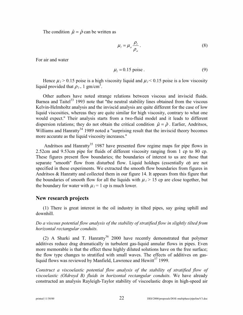
The condition ρµ ˆˆ = can be written as

a

lal ρρµµ = . (8)

For air and water

poise15.0=lµ . (9)

Hence µ l > 0.15 poise is a high viscosity liquid and µ l < 0.15 poise is a low viscosityliquid provided that ρ l ≈ 1 gm/cm3.

Other authors have noted strange relations between viscous and inviscid fluids.Barnea and Taitel33 1993 note that ''the neutral stability lines obtained from the viscousKelvin-Helmholtz analysis and the inviscid analysis are quite different for the case of lowliquid viscosities, whereas they are quite similar for high viscosity, contrary to what onewould expect.'' Their analysis starts from a two-fluid model and it leads to differentdispersion relations; they do not obtain the critical condition ρµ ˆˆ = . Earlier, Andritsos,Williams and Hanratty34 1989 noted a ''surprising result that the inviscid theory becomesmore accurate as the liquid viscosity increases.''

Andritsos and Hanratty35 1987 have presented flow regime maps for pipe flows in2.52cm and 9.53cm pipe for fluids of different viscosity ranging from 1 cp to 80 cp.These figures present flow boundaries; the boundaries of interest to us are those thatseparate ''smooth'' flow from disturbed flow. Liquid holdups (essentially α) are notspecified in these experiments. We extracted the smooth flow boundaries from figures inAndritsos & Hanratty and collected them in our figure 14. It appears from this figure thatthe boundaries of smooth flow for all the liquids with µ l > 15 cp are close together, butthe boundary for water with µ l = 1 cp is much lower.

New research projects

(1) There is great interest in the oil industry in tilted pipes, say going uphill anddownhill.

Do a viscous potential flow analysis of the stability of stratified flow in slightly tilted fromhorizontal rectangular conduits.

(2) A Sharki and T. Hanratty36 2000 have recently demonstrated that polymeradditives reduce drag dramatically in turbulent gas-liquid annular flows in pipes. Evenmore memorable is that the effect these highly diluted solutions have on the free surface;the flow type changes to stratified with small waves. The effects of additives on gas-liquid flows was reviewed by Manfield, Lawrence and Hewitt37 1999.

Construct a viscoelastic potential flow analysis of the stability of stratified flow ofviscoelastic (Oldroyd B) fluids in horizontal rectangular conduits. We have alreadyconstructed an analysis Rayleigh-Taylor stability of viscoelastic drops in high-speed air


streams at ultra high Weber numbers. We used an Oldroyd B model. The analysis can befit to the observations by the selection on very small retardation times.

There is controversy about drag reduction in dilute polymer solutions and perhaps themajority think it can't be explained by Oldroyd B models. However our very accuratecalculations do give rise to drag reductions matching experiment (Min, Yoo, Choi andJoseph38 2000).

(3) There is no analysis of stability in round pipes that respect the geometry of thepipe by enforcing the condition that the pipe wall is a streamline. This is a difficultproblem that is much simpler but still difficult in the context of viscous potential flow inwhich the potential φ=satisfies Laplace's equations. If x is the axis and r, θ=are polarcoordinates in the cross section, we look for eigenfunctions

φ (r,θ,x,t) = eσ=teikxΦ=(r,φ,k)

such that

( ) 0,, =∂Φ∂ kar

θ

where r = a is the pipe wall. The determination of representations of the functions Φabove and below the flat free surface at y = 0 is not straightforward and is the mainobstacle to be overcome.

X Nonlinear effects. Bifurcation analysis of KH instabilityusing viscous potential flow. Multiple solutions. There is no theory that is faithful to all conditions at play in experiments. None of the

theories agree with experiments. Attempts to represent the effects of viscosity are onlypartial, as in our theory of viscous potential flow, or they require empirical data on walland interfacial friction, which are not known exactly and may be adjusted to fit the data.Some choices for empirical inputs underpredict and others overpredict the experimentaldata.

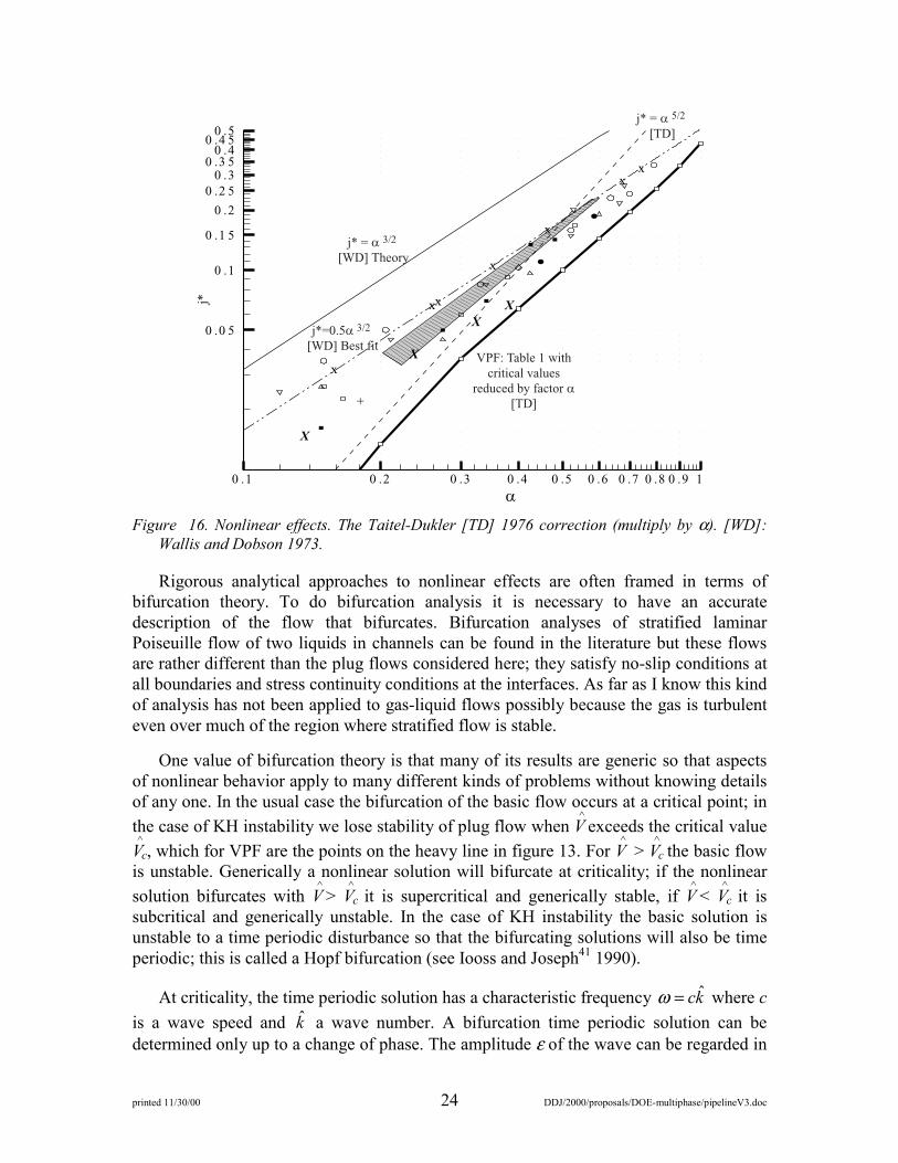
It is widely acknowledged that nonlinear effects at play in the transition fromstratified to slug flow are not well understood. The well-known criteria of Taitel andDukler39 1976, based on a heuristic adjustment of the linear inviscid long wave theory fornonlinear effects, is possibly the most accurate predictor of experiments. Their criterionreplaces j* = α 3/2 with j* = α 5/2. We can obtain the same heuristic adjustment fornonlinear effects on viscous potential flow by multiplying the critical value of velocity infigure 13 by α. Plots of j* = α 3/2, j* = α 5/2 and the heuristic adjustment of viscouspotential flow, together with the experimental values of Wallis and Dobson24 1973, andKordyban and Ranov40 1970 are shown in figure 16. The good agreements in evidencethere lacks a convincing foundation.


X

X

XX

+

x

xx

x

x

xx

a

j*

0 .1 0 .2 0 .3 0 .4 0 .5 0 .6 0 .7 0 .8 0 .9 1

0 .0 5

0 .1

0 .1 5

0 .2

0 .2 5

0 .30 .3 5

0 .40 .4 5

0 .5

j* = a 3/2

[WD] Theory

j*=0.5a 3/2

[WD] Best fit

j* = a 5/2

[TD]

VPF: Table 1 with

critical values

reduced by factor a

[TD]

Figure 16. Nonlinear effects. The Taitel-Dukler [TD] 1976 correction (multiply by α). [WD]:Wallis and Dobson 1973.

Rigorous analytical approaches to nonlinear effects are often framed in terms ofbifurcation theory. To do bifurcation analysis it is necessary to have an accuratedescription of the flow that bifurcates. Bifurcation analyses of stratified laminarPoiseuille flow of two liquids in channels can be found in the literature but these flowsare rather different than the plug flows considered here; they satisfy no-slip conditions atall boundaries and stress continuity conditions at the interfaces. As far as I know this kindof analysis has not been applied to gas-liquid flows possibly because the gas is turbulenteven over much of the region where stratified flow is stable.

One value of bifurcation theory is that many of its results are generic so that aspectsof nonlinear behavior apply to many different kinds of problems without knowing detailsof any one. In the usual case the bifurcation of the basic flow occurs at a critical point; inthe case of KH instability we lose stability of plug flow when V

^ exceeds the critical valueV^ c, which for VPF are the points on the heavy line in figure 13. For V

^ > V^ c the basic flow

is unstable. Generically a nonlinear solution will bifurcate at criticality; if the nonlinearsolution bifurcates with V

^ > V^ c it is supercritical and generically stable, if V

^ < V^ c it is

subcritical and generically unstable. In the case of KH instability the basic solution isunstable to a time periodic disturbance so that the bifurcating solutions will also be timeperiodic; this is called a Hopf bifurcation (see Iooss and Joseph41 1990).

At criticality, the time periodic solution has a characteristic frequency kc ˆ=ω where cis a wave speed and k a wave number. A bifurcation time periodic solution can bedetermined only up to a change of phase. The amplitude ε of the wave can be regarded in


the bifurcation parameter; it can be positive or negative and is conveniently described byprojections on the null spaces of the adjoint operator (Iooss and Joseph, Chapter VII).

We may formulate the bifurcation analysis in a frame moving with water; the UV =ˆis the velocity of air. We seek a bifurcating solution U(ε ) with a frequency ω(ε ) obtainedby scaling time tt ∂∂=∂∂ /ˆ/ ω and write the governing equations for viscous potentialflow with potential φ as follows:

0,,ˆ 2 =∇=∇+=∇ φφεφ UU xeU

It is understood that each equation must be written twice, for the gas with parameters(U, µg, ρg) and the liquid (0, µl, ρ=l).

( ) px

Ut

−∇=

∇∇+∂∂+

∂∂∇ 2

2φεφφωρ

On the interface z = h(x,y,t) we have

∂∂

∂∂+

∂∂

∂∂+

∂∂+

∂∂=

∂∂

yh

yxh

xxhU

th

zφφεωφ

and

Hghnxx

np jji

2]][[42

2 γρφµ −=+

⋅∂⋅∂∂⋅+−

where H is twice the mean curvature and, for example

[[ρ]] = ρg - ρ=l

We seek a solution as a power series in ε. It can be shown the U(ε) and ω(ε) are evenfunctions (Iooss & Joseph, Chapter III). It follows that periodic solutions that bifurcate toone or the other side of criticality, as in figure 18, and never to both sides; periodicbifurcating solutions cannot undergo two-sided bifurcation.

It is of interest to speculate how some outstanding experimental observations on theloss of stability of stratified flow may be explained by bifurcation. First, we recall thatWallis and Dobson 1973 reported very robust data on premature slugging, slugs whenV^ < V

^ c . Andritsos and Hanratty 1987 report that stratified flow loses stability to regularwaves when the viscosity is small, and directly to slugs when the viscosity is large.Premature waves would be described by subcritical bifurcation as in the diagram offigure 17. A supercritical fabrication to regular waves is shown in figure 18. Perhapsthere is a change from supercritical to subcritical bifurcation as the viscosity is increasedin the experiments of Andritsos and Hanratty. Many other bifurcation scenarios arepossible.


WaveAmplitude

Stable StratifiedFlow

Stable Slug

Unstable Slug

V^ c

V^

Unstable

Figure 17. A speculative diagram ofsubcritical bifurcation to explainpremature slugging.

WaveAmplitude

Stratified Flow

V^ c

V^

Figure 18. A speculative diagram ofsubcritical bifurcation to explain thesupercritical bifurcation of regular waves.

XI Rise velocity of long gas bubbles in pipes and conduitsWe propose to do studies to explain many unexplained and even paradoxical results

for long gas bubbles, called slugs, rising in liquids in vertical pipes and conduits. Suchbubbles form when the gas input is large. These kinds of bubbles can arise naturally bycoalescence of small bubbles following in the wake of large gas bubbles. The formationof slugs in vertical pipelines is an important feature in the extraction of oil from a verticalwell bore. The pressure depletion along the pipe will cause dissolved gases like methaneand carbon dioxide to come out of solution and join the already existing gas phase.

U

θ0

qs

y

θ

Figure 19. Spherical cap bubble

The properties of slugs, even in stillliquids, which is the easiest, are reallyamazing. First of all, the rise velocity ofthe bubble can be predicted without anydynamic force balance, from the shape ofthe bubble alone. Secondly, the risevelocity is independent of the length of thebubble so that the usual idea based onArchidmedes principle seems not to applyhere. The rise velocity of the Taylor-Davies42 bubble and the spherical capbubble, which was also analyzed by them,is determined by the shape of the bubble.When the radius R = D/2 of the bubble is

not too small surface tension may be neglected and the pressure in the gas and on thespherical cap is constant. The Bernoulli equation on the cap is given by

[ ]θθ cos)(22 rRgqs −=− . For potential flow over a sphere θsin232 Uqs = . Looking near

the stagnation point with r(θ) = R, sin θ = θ, cos θ = 1-θ=2 /2 they find


32, == KgDKU (10)

where K is a shape factor. Batchelor notes that

the remarkable feature of [equations like (10)] and its various extensions is that the speedof movement of the bubble is derived in terms of the bubble shape, without any need forconsideration of the mechanism of the retarding force which balances the effect of thebuoyancy force on a bubble in steady motion. That retarding force is evidentlyindependent of Reynolds number, and the rate of dissipation of mechanical energy isindependent of viscosity, implying that stresses due to turbulent transfer of momentumare controlling the flow pattern in the wake of the bubble43.

The rise of a Taylor bubble is similar, but slightly lower, with an empirical of K about0.35. The formula (10) for the rise velocity is independent of the length of the bubble, itis independent of the gas or liquid density or viscosity.

Another paradoxical property is that the Taylor bubble rise velocity does not dependon how the gas is introduced. In the Taylor-Davies experiments the bubble column isopen to the gas. In other experiments the gas is injected into a column whose bottom isclosed.

There are many studies of the effects of liquid of viscosity µ, pipe diameter, densityρ, and surface tension on the rise velocity of Taylor bubbles. Correlations by White andBeardmore44 1962, and Brown45 1965, who gives

2/12/1

2/1)1(135.0

−+−=

NDNDgDU (11)

where3/1

2

2

5.14

=

µρ gN .

Equation (11) gives accurate results when ND > 120 and it reduces to (10) when the lastterm in (11) is much less than 1.

Why doesn’t the rise velocity depend on the length of the Taylor bubble? If a Taylorbubble rises in steady flow it must be in a balance between buoyant weight and drag. Wedon't know how to compute either. If we think of Achimedes principle we would be ledto think that the buoyant would increase with volume accordingly (ρl-ρg)g. Volume andthe bubble would rise faster, just as large spherical bubbles rise faster than small one.Archimedes principle requires that the pressure of the hydrostatic impress itself on thebubble. Evidently this does not occur in the Taylor bubble.

The liquid at the wall drains under gravity without changing the pressure. Theequation is


=∂∂

dxdpg

xU

l no2

2

ρµ (12)

Then the cylindrical part of the long bubble is effectively not displacing liquid (doesn’tchange pressure). The buoyancy is still the volume of the hemisphere poking into theliquid at the top. The equation of motion buoyancy = drag doesn’t change.

x

Figure 20. Drainage at the wall of a rising Taylor bubble. If -U is added to this system the wallmoves and the bubble is stationary.

Rise velocity in annular pipes. Another paradoxical result is that if a Taylor bubble risesin the annular space between two cylinders, it will rise faster than it would if the innercylinder were absent. Caetano, Shoham and Brill46 1992 studied the rise of gas bubbles inannular pipes; they note that

For any combination of fluid pairs and annuli configurations., the Taylor bubble risevelocity is larger than predicted for a circular pipe with a diameter equal to the annulusshroud diameter. As in the circular pipe case, once the bubble cap is developed, thebubble rise velocity is insensitive to the bubble length and/or volume.

Moreover, if the perimeter of the annular increased while the radius of the outer cylinderis fixed, so that the gap between the cylinders decreases, the Taylor bubble will rise stillfaster. Radar, Bourgoyne and Ward47 1975 did experiments in a small scale apparatus andin a 6000 ft. deep well. They used water, water-glycerin and non-Newtonian fluids andair, methane and penthane as gas. They say (pg. 574) "…It was surprising that, at first,the gas bubble rose faster when the inner tube was present… More surprising was that thebubble rose even faster when the annular cross-sectional area was further reduced byincreasing the diameter of the inner tube."

Bubble rise with insertions. Bubble rise velocities in configurations with and withoutinsertions were studied by Grace and Harrison48 (1967). They studied bubbles of Taylortype, but smaller ones, big enough to have an ellipsoidal shape but not so big as todisplay Taylor bubble behavior. Their basic experimental configuration was a verticalduct with a rectangular cross-sectional area. The insertions consisted of single or multiplerods, flat plates and rectangular cross section area ducts. They found that a bubble


changes its shape from a circular-cap to an elliptical-cap and, in the limit, to a parabolic-cap shape. These new shapes are a function of the particular surface inserted, and providefaster rising velocities as compared to flow without insertions.

Research questions. We are interested in Taylor bubbles and especially when they rise inoils of high viscosity. Brown 1965 and White and Beardmore49 1962 have shown that incertain circumstances Taylor bubbles in high viscosity liquids, as high as 450 cp will riseat the speed gD35.0 of gas bubbles in water. The questions asked below are meant tobe qualified by a specification of parameters for which they are appropriate.

• When and why is the rise velocity of the Taylor bubble independent of volume?

• When and why is the rise velocity of the Taylor bubble the same whether thebottom of the column is open or closed?

• How is bubble shape connected with wall drainage?

• How does the bubble rise velocity change with the gap size in the annulus and withdrainage area on both cylinder walls?

• What is the mechanism by which inserts increase the rise velocity of Taylorbubbles?

• Is there an optimal position, type and placement of inserts for the fastest rise ofTaylor bubbles in a tube with inserts?

• What is the force balance that controls the rise velocity of a Taylor bubble?

• What is the effect on all the above questions and the dynamics of Taylor bubblesgenerally of upflow and downflow of the liquid?

Experiments indicate that Taylor bubbles in concentric annuli are unstable. Observed gasbubbles only partially fill the annulus45,46.

• To what extent are nonaxisymmetric shapes of bubbles stable and unique inperfectly concentric annuli?

• Compare the rise velocity of axisymmetric and nonaxisymmetric bubbles inannuli.

Research projects

The projects we propose are motivated by the research questions posed above. Weplan to attack these projects with experiments and numerical simulations.

Experiments: In the Minnesota lab we will do experiments on the effects of inserts onTaylor bubbles in water. A diagram of this kind is shown below as figure 21. We willalso consider the case in which the flat plate extends to the bottom of the bubble column.


Flat plate

Figure 21. Diagram of the effect of a splitter plate on the rise velocity of a Taylor bubble.

The effects of upflow and downflow of water on the rise velocity of Taylor bubbleswill be studied in the apparatus described in figure A.1.

Experiments of a similar type, using oils, will be carried out in Venezuela, using theirexcellent apparatus shown in figure A.3.

Numerical simulation

Numerical studies of Taylor bubbles rising through stagnant liquids have been givenby Mao and Dukler50 1990 and by Bugg, Mack and Rezkallah51 1998. The Bugg et alpaper covers a wider range of conditions and makes no a priori assumption about theshape of the leading edge or the terminal speed. They use a volume of fluid method anddo extensive calculations for different values of the Froude Eötvös and Morton numbers.They obtain some reasonable agreement with experiments in the literature. They do notaddress the research questions posed in the previous section and they neglect surfacetension.

The simulation project being proposed here is based on level set method based on afully resolved Navier Stokes solver with no approximations developed by P. Singh 1999,2000. This code has been programmed and preliminary results are shown in figures 22.


(a) (b) Figure 22. The direct numerical approach is used to simulate the motion of an air bubble rising

in a two-dimensional channel filled with a liquid of viscosity 1.0 CGS units. The channelwidth is 1 cm and the bubble length is approximately 4 cm. The initial bubble width is 0.8 cm.The steady state bubble shape and streamlines are shown. (a) t = 0.001 (b) t = 0.01.

In the level set method, the interface position is not explicitly tracked, but is defined to bethe zero level set of a smooth function φ,==which is assumed to be the signed distancefrom the interface. Along the interface it is assumed to be zero. In order to track theinterface, the level set function is advected according the velocity field. One of theattractive features of this approach is that it is relatively easy to implement in both twoand three dimensions. In fact, an algorithm developed for two dimensions can be easily


generalized to three dimensions. Also, the method does not require any special treatmentwhen a front splits into two or when two fronts merge.

Our level set code is fully 3D; unlike previous numerical approaches (Mao et all1990, Bugg et al 1998) it is not restricted to axisymmetric flow. This code can be used toaddress all of the questions posed above.


XII Appendix A -Experimental facilities

The Minnesota laboratory has two horizontal 1" diameter × 240" long pipelines; oneis equipped for simultaneous injection of water and oil and the other is equipped forstudies of pipelining of bitumen froth. The froth line is jacketed in a plastic tube in whichcooling water can be circulated. A vertical 0.48D vertical U loop, 180" high is used tostudy vertical up and down flow. Many measuring devices are available for our use, suchas high-speed and high-resolution video cameras, analytical software for imageprocessing and a wide range of rheometers. We plan to use these lines in studies offrictional heating of core-annular flow. We will be comparing data from the Minnesotalab with data from Syncrude's 36" commercial line.

For studies of Taylor bubbles we haveconstructed a 2" vertical transparent bubblecolumn 10 meters high (figure A.1). Thefrequency controller can deliver water flowrates from 0.3 m/s to 1.3 m/s.

Figure A.1. (right) Bubble column schematic.Fl

exib

le h

ose

Ultr

ason

ic fl

owm

eter

Tank

PPressureGauge

Frecuencycontroler

10 m

5 m

9 m

2" pipe

Flow

gas flow

The Minnesota lab is not equipped to do experiments on gas-heavy oil flow. The oilsare environmentally unfriendly and the pipelines are expensive. We are going to carry outthe experiments on heavy oils with viscosities from 130 to 1200 cp at the experimentalfacility of PDVSA / Intevep in Los Teques, VZ. Their D = 2" horizontal flow loop is1253D total length, 835D entrance region and 250D test section which is transparent andfully instrumented. The loop is to run with VSL < 3 m/s and VSG < 10 m/s (see figure A.2).

The experimental apparatus is shown in figure A.3. It consists of a transparent acryliccolumn with an inside diameter of 3 in. and a total height of approximately 2.5m. At thebottom of the column a transparent acrylic box is connected. The box has a hemisphericalcup held above an injection nozzle. This nozzle is connected to a syringe using tubing. Inorder to obtain the desired bubble volume air is added into the cup, by injecting airrepeatedly with the small syringe. The bubble is released by inverting the cup. Thismechanism allows the formation of small bubbles (0.8 ml) and Taylor bubbles (300 ml).


To measure the bubble's velocity, the rising bubble is recorded with a high speed videocamera NAC HSV 1000, which acquires 500 to 1000 frames per second. This video isdigitized and processed by a program developed in PDVSA Intevep using the IMAQVision for LabView.

Figure A.2. Horizontal flow loop in Venezuela laboratory.1253D total length, 2 in., 835D

entrance region, 250D test section. Fully transparent test section, fully instrumented andadvance Scada with slug tracking. VSL < 3 m/s and VSG < 10 m/s, µ0 = 134, 481, 754, 1180cp.

Figure A.3. Vertical flow loop in Venezuela laboratory. 65 ft. long, annulus I.D. 3", internal rod1". QL = 30-4000 BPD, QG = 1.2-1200 MSCF/D. µ0 = 134, 481, 754, 1180 cp. Fullytransparent test section, fully instrumented and advance Scada.

XIII Appendix B – Shear stress transport (SST) turbulencemodelConsider two concentric immiscible fluids flowing down an infinite horizontal

pipeline. We assume that the core is axisymmetric with interfacial waves that are periodicalong the flow direction; the pressure in periodic fully developed flows can be expressedas

),(),( rxpxrxP +−= β , (B-1)

where β is a mean pressure gradient and p(x,r) represents the periodic part of the wholepressure P and behaves in periodic fashion from module to module. The term βxindicates the general pressure drop along the flow direction.


The continuity equation and Navier-Stoke equation for the unsteady incompressibleflow in cylindrical coordinate can be written as follows:

continuity

0)(1)( =∂∂+

∂∂ vr

rru

xρρ , (B-2)

x-momentum

∂∂

∂∂+

∂∂−=

∂∂+

∂∂+

∂∂

xu

xxp

ruv

xuu

tu

eff 2µβρxk

ru

xvr

rr eff ∂∂−

∂∂+

∂∂

∂∂+

321 ρµ , (B-3)

r-momentum

∂∂+

∂∂

∂∂+

∂∂−=

∂∂+

∂∂+

∂∂

ru

xv

xrp

rvv

xvu

tv

effµρxk

rv

rvr

rr effeff ∂∂−−

∂∂

∂∂+

32221

2 ρµµ ,

(B-4)where

Teff µµµ += , );31.0max(

31.0

2Fk

T Ω=

ωρµ ,

and Ω is the absolute value of the vorticity.The turbulent kinetic energy equation and the dissipation rate equation are obtained

from Menter’s shear stress transport model (F. R. Menter 1994). The SST model utilizesthe original k-ω model of Wilcox in the inner region of the boundary layer and switchesto the standard k-ε model in the outer region of the boundary layer and in free shearflows. In the dissipation rate equation, the function F1 is designed to be one in the nearwall region (activating the original model) and zero away from the surface (activating thetransformed model). Then the turbulent kinetic energy and the dissipation rate equationmodified by SST model are written as

turbulent kinetic energy

( )

∂∂+

∂∂+=

∂∂+

∂∂+

∂∂

xk

xP

rkv

xku

tk

Tkk µσµρ ( ) ωρβµσµ krkr

rr Tk*1 −

∂∂+

∂∂+ , (B-5)

dissipation rate

( ) 2βρωµγρωµσµωωωρ ω −+

∂∂+

∂∂=

∂∂+

∂∂+

∂∂

kT

T Pxxr

vx

ut

( ) ( )xx

kFr

rrr T ∂

∂∂∂−+

∂∂+

∂∂+ ω

ωρσωµσµ ωω

112121 ( )

rrkF∂∂

∂∂−+ ω

ωρσω

112 21 , (B-6)

where


∂∂+

∂∂+

+

∂∂+

∂∂=

2222

2ru

xv

rv

rv

xuP Tk µ .

Let φ1 represent a constant in the original k-ω model (σk1,…), φ2 a constant in thetransformed k-ε model (σk2,…). The corresponding constant φ of the new model (σk,…)is given as follows:

2111 )1( ΦΦΦ FF −+= . (B-7)

The constants of set 1 (φ1) and set 2 (φ2) are

σk1 = 0.85, σw1 = 0.5, β1 = 0.075, κ = 0.41, = *21

*11 βκσββγ ω−= ,

σk2 = 1.0, σw2 = 1.856, β2 = 0.0828, β∗===0.09,= *22

*21 βκσββγ ω−= ,

and F1 and F2 are given by

)tanh(arg411 =F ,

= 2

221

4;500;

09.0maxminarg

yCDk

yyk

kω

ωρσρωµ

ω,

∂∂

∂∂= −20

2 10;12maxjj

k xxkCD ω

ωρσωω , )tanh(arg2

22 =F ,

=

ρωµ

ω 22500;

09.0maxarg

yyk ,

where y is the distance to the next surface.


XIV References

The first ten references are listed in section II on page 4 of the text.

11 D.D. Joseph & Y. Renardy, 1992. Fundamentals of Two-Fluid Dynamics. Part II, IAM412 D.D. Joseph, R. Bai, K.P. Chen & Y. Renardy, 1997. Core-annular flows, Annular Rev. Fluid

Mech. 21, 65-90. This paper gives an overview of the issues posed by the science andtechnology of transporting heavy oil in a sheath of lubricating water. It touches on measuresof energy efficiency, industrial experiences, fouling, stability, models of levitation and futuredirection.

13 V. Kruka, 1977. Method for establishing Core-Flow in Water-in-Oil Emulsions or dispersionsCanadian patent granted to Shell Canada, No. 1008108.

14 O. Neiman, K. Sury, D.D. Joseph, R. Bai and C. Grant, 1999. Process for pumping bitumenfroth through a pipeline, US Patent 5,988,198.

15 O Neiman . 1986. Froth pipelining tests. Syncrude Canada Research and DevelopmentProgress Report. 15(1):373-407.

16 DD Joseph, R Bai, C Mata, K Sury & C Grant, 1999. Self-lubricated transport of bitumen froth,J. Fluid Mech. 386, 127-148.

17 R Bai, K Kelkar, DD Joseph, 1996. Direct simulation of interfacial waves in a high-viscosity-ratio and axisymmetric core-annular flow. J. Fluid Mech. 327, 1-34.

18 R Bai, K Chen and DD Joseph, 1992. Lubricated pipelining: stability of core-annular flow. Part5, experiments and comparison with theory. J. Fluid Mech. 240, 97-142.

19 J Li, Y Renardy, 1999. Direct simulation of unsteady axisymmetric core-annular flow with highviscosity ratio. J. Fluid Mech. 391, 123-149.

20 R Bai & DD Joseph, 2000. Steady flow and interfacial shapes of a highly viscous dispersedphase, Int. J. Multiphase Flow, 26, 1469-1491.

21 T Ko, HG Choi, R Bai and DD Joseph, 2000. Turbulent wavy core-annular flow simulationusing a k-ω turbulence model and finite element method, in progress.

22 FR Menter, 1994. Two-equation eddy-viscosity turbulence models for engineering applications.AIAA Journal, 32(8), 1598-1605.

23 R Chokshi, Z Schmidt, D Doty. May 1996. Experimental Study and the Development of aMechanistic Model for Two-Phase flow Through Vertical Tubing. SPE 35676. WesternRegional Meeting, Alaska, pp 255-267.

24 L Gómez, O Shoham, Z Schmidt, R Chokshi, A. Brown, T. Northug October 1999. A UnifiedModel for Steady Two-Phase Flow in Wellbores and Pipelines. SPE 56520, SPE AnnualTechnical Conference and Exhibition, Houston, Texas, pp 307-320.

25 J.M. Mandhane, G.A. Gregory and K. Aziz, 1974, A flow pattern map for gas-liquid flow inhorizontal pipes. Int. J. Multiphase Flow 1, 537-551.


26 PY Lin & TJ Hanratty, 1987. Effect of pipe diameter on flow patterns for air-water flow in

horizontal pipes, Int. J. Multiphase Flow, 13(4), 549-563.27 G.B. Wallis and J.E. Dobson, 1973. The onset of slugging in horizontal stratified air-water

flow. Int. J. Multiphase Flow, 1, 173-193.28 C.J. Crowley, G.H. Wallis and J.J. Barry, 1992. Validation of a one-dimensional wave model

for the stratified-to-slug flow regime transition, with consequences for wave growth and slugfrequency. Int. J. Multiphase Flow. 18(2), 249-271.

29 DD Joseph and TY Liao, 1994. Potential flows of viscous and viscoelastic fluids, J. FluidMech. 265, 1-23.

30 D.D. Joseph, J. Belanger and G.S. Beavers, 1999. Breakup of a liquid drop suddenly exposed toa high-speed airstream, Int. J. Multiphase Flow 25, 1263-1303.

31 DD Joseph, TS Lundgren, T Funada, 2000. Viscous Potential Flow Analysis of Kelvin-Helmholtz Instability, http://www.aem.umn.edu/people/faculty/joseph/.

32 T Funada and DD Joseph, 2000. Viscous potential flow analysis of Kelvin-Helmholz instabilityin a channel, Submitted to Int. J. Multiphase Flow; alsohttp://www.aem.umn.edu/people/faculty/joseph/.

33 D. Barnea, and Y. Taitel, 1993. Kelvin-Helmholtz stability criteria for stratified flow: viscousversus non-viscous (inviscid) approaches, Int. J. Multiphase Flow 19, 639-649.

34 N. Andritsos, L. Williams and T.J. Hanratty, 1989. Effect of liquid viscosity on the stratified-slug transition in horizontal pipe flow. Int. J. Multiphase Flow, 15, 877-892.

35 N. Andritsos and T.J. Hanratty, 1987. Interfacial instabilities for horizontal gas-liquid flows inpipelines, Int. J. Multiphase Flow, 13, 583-603.

36 Al Sharki and TJ Hanratty, 2000. Effect of drag reducing polymers on annular gas-liquid flowin a horizontal pipe, Int. J. Multiphase Flow, to appear.

37 CJ Manfield, C Lawrence and G Hewitt, 1999. Drag reduction with additives in multiphaseflow: a literature survey. Multiphase Science and Technology, 11, 197-221.

38 T Min, JY Yoo, H Choi and DD Joseph, 2000. Direct numerical simulation of turbulent dragreduction by polymer additive. DFD00 meeting of the American Physical Society. To bepublished.

39 Y. Taitel and A.E. Dukler, 1976. A model for predicting flow regime transitions in horizontaland near horizontal gas-liquid flow. AIChE J., 22, 47-55.

40 E.S. Kordyban and T. Ranov, 1970. Mechanism of slug formation in horizontal two-phaseflow. Trans. ASME J. Basic Engng., 92, 857-864.

41 G Iooss and DD Joseph, 1990. Elementary Stability and Bifurcation Theory. Springer, 2nd

edition.42 RM Davies and GI Taylor 1950. The mechanism of large bubbles rising through liquids in

tubes, Proceedings of the Royal Society, 200(A), 375-390.


43 G.K. Batchelor 1967, An Introduction to Fluid Dynamics, Cambridge University Press, page

477.44 ET White and RH Beardmore 1962. The velocity of rise of single cylindrical air bubbles

through liquids contained in vertical tubes. Chem. Eng. Sci. 17, 351-361.45 RAS Brown 1965. The mechanics of large gas bubbles in tubes, I. Bubble velocities in stagnant

liquids. The Canadian Journal of Chemical Engineering, October, pp 217.46 EF Caetano, O. Shoham and JP Brill, 1992. Upward vertical two-phase flow through an

annulus--Part I: Single-phase friction factor, Taylor bubble rise velocity, and flow patternprediction. J. Energy Resources Tech., 114, 1.

47 EW Radar, AT Bourgoyne and RH Ward, 1975. Factors affecting bubble rise velocity gaskicks. J. Pet. Tech. 27, 571-584.

48 JR Grace and D Harrison, 1967. The influence of bubble shape on the rising velocities of largebuble, Chemical Engineering Science. 22, 1337-1347.

49 ET White and RH Beardmore, 1962. The velocity of rise of single cylindrical air bubblesthrough liquids contained in vertical tubes. Chem. Eng. Sci. 17, 351-361.

50 Z-S Mao and AE Dukler, 1990. The motion of Taylor bubbles in vertical tubes. I. A numericalsimulation for the shape and rise velocity of Taylor bubbles in stagnant and flowing liquids.J. Comp. Phys. 91, 132-160.

51 JD Bugg, K Mack and KS Rezkallah, 1998. a numerical model of Taylor bubbles risingthrough stagnant liquids in vertical tubes, Int. J. Multiphase Flow, 24(2), 271-281.

Multiphase Pipelining - AEM · does not seem to be a literature on frictional heating in turbulent...

Documents

Transcript of Multiphase Pipelining - AEM · does not seem to be a literature on frictional heating in turbulent...