Single and Multiphase Flow and Transport in Fractured Porous Media STANFORD THESES
Multiphase Flow in Porous /Fracture MediaMultiphase Flow in Porous /Fracture Media
M S Mohan KumarMini Mathew & Shibani jhaM S Mohan KumarMini Mathew & Shibani jhajDept. of Civil EngineeringIndian Institute of Science
jDept. of Civil EngineeringIndian Institute of ScienceBangalore, IndiaBangalore, India

2 Multiphase fluids ----Fluids which are immiscible and isslightly soluble.Represent as individual phase in the subsurface, flow behavior is described asmultiphase problemmultiphase problem.Common trait of these substance are NAPLs
2 NAPLs -- ----- LNAPLsDNAPL------- DNAPLs
2 The phase does not fill the pore space completely.
2 Multiphase flow--- Simultaneous flow of more than two fluids, does not take place as a piston like process.
2 Flow experiments show that Darcy’s law can be extended for multiphase flows
2 D ’ l it f h h i di i d ib d2 Darcy’s velocity for each phase in a porous medium is described by the generalized Darcy’s law.
2 Subsurface leakage of hydrocarbon fuels and other immiscible Source of NAPLsSource of NAPLs
organic liquids due to leaky storage tanks or pipelines.
2 Coal tar from illuminating gas production, wastes from steelCoal tar from illuminating gas production, wastes from steel industry and wood treating operation
2 O i b t d i i d t i Mi l f l2 Organic substances used in industries as Mineral fuels ( ex : Petrol, fuel oil etc), Solvents Detergents ( ex : Chlorinated hydrocarbons)
GoalGoal2 Estimate the potential danger of NAPL infiltration
& to plan eventual remediation techniques.
2 To reduce the field investigation effort and cost.

2 Vertical migration in the vadose gzone predominantly by gravity
2 Some lateral spreading due to capillarforces and media propertiesforces and media properties
2 Migration occurs when enough pressure is available to over come pthe displacement pressure
2 In saturated zone the movement is bydisplacement of waterdisplacement of water
2 In saturated medium ---- 2 phase systemIn saturated medium 2 phase system
2 In unsaturated medium ----- 3 phase system or------ 2 phase system with static air pressure
General migration pattern and process of NAPLs (after Helmig)General migration pattern and process of NAPLs (after Helmig)

Air
Processes of Multiphase Multicomponent SystemProcesses of Multiphase Multicomponent System
Water Air
AirWatervapour
Water Organiccompound
p
Organiccompound
Air
NAPL
Air
Water
NAPL
NAPL Water
NAPL
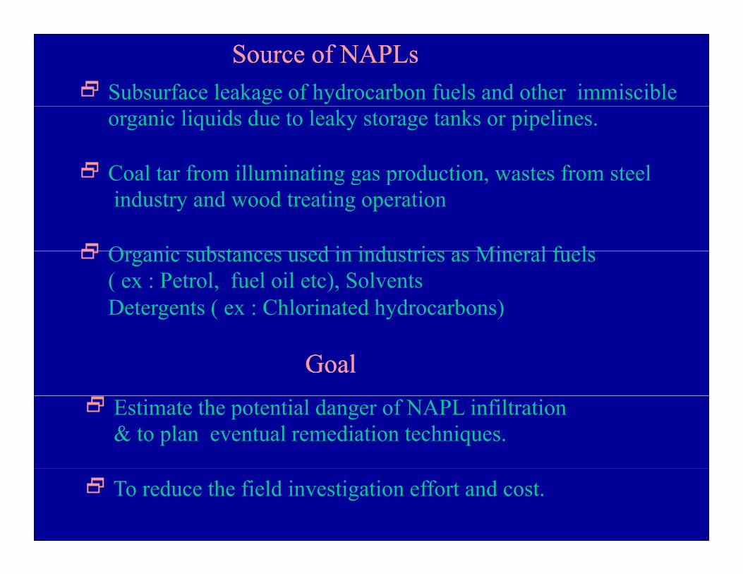
Multiphase Multicomponent Flow in the Subsurface -Governing Equations
Multiphase Multicomponent Flow in the Subsurface -Governing EquationsGoverning EquationsGoverning Equations
] 0dGqρ)vρ(φdivt
)ρφ()vρ,L(φ αααααG
αααα,α =−+⎢⎣
⎡∂
∂= ∫
{ } ] 0dGr)Xgrad(ρDSφXvρdiv)XρS(φ
)XL(v kα
kαα
kpmαα
kααα
kαααk
αα =−−+⎢⎢⎡
∂
∂=∫ { } ]
vv
)g(ρφρt
)( αααpmαααααG
αα,⎢⎢⎣ ∂∫
DSδvvv
)α(αvαδDSφ 10/3α
3/4ij
jiTLLjiαpm
kα ji +−+= ϕ
[ { } { } ] 0rTgradλdiv)ρPu(ρvdiv
t)Sρ(u
tTcρ)φ(1T)PL(u αpm
α
αααα
αααs
Gs
N
1αα,α, =−+++
∂∂
+∂∂
−= ∫∑=
ϕ
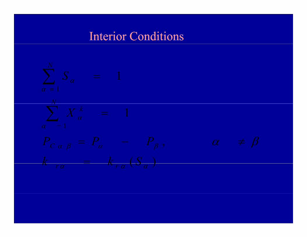
Interior ConditionsInterior Conditions
1SN
∑ 11α
αS
N
=∑=
11α
αXN
k =∑=
)(
,βαβα βα
Skk
PPPC=
≠−=
)( ααα Skk rr

Present study consists ofPresent study consists of
2Modelling and analysis of NAPLs migration in saturated porous medium----two phase NAPL-Water system
2 Study the influence of air phase on the infiltration of waterin unsaturated porous medium ---- two phase Air-Water system.
2Modelling and analysis of NAPL migration in unsaturated porous mediumin unsaturated porous medium.
Three phase Air-NAPL-Water systemTwo phase NAPL-Water system with constant air pressure
2Modelling and analysis of NAPL migration in combined saturated-unsaturated porous medium
2 Parallel computation of multiphase flow in saturated porous medium
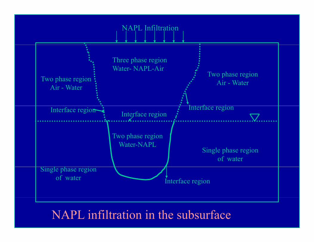
NAPL Infiltration
Three phase regionWater- NAPL-Air
Two phase regionTwo phase regionAir - WaterTwo phase region
Air - Water
I t f i
Two phase region
Interface regionInterface regionInterface region
Si l h i
Single phase regionof water
Two phase regionWater-NAPL
Single phase regionof water Interface region
NAPL infiltration in the subsurface

Two Phase NAPL-Water Simulation in Saturated Porous MediaTwo Phase NAPL-Water Simulation in Saturated Porous Media
2 Develop a robust model and numerical method for the simulation of NAPL-Water in saturated porous media
2 Models of all the combinations of pressures and saturations of the phases have been developed
2 Comparative study is made between 6 models with simultaneous and modified sequential methods.
2 Comparative study between conventional simultaneous,modified sequential, and adaptive solution fully implicitmodified sequential, and adaptive solution fully implicitmodified sequential methods using pressure and saturationof wetting fluid are made
2 Effect of different types of approximations of nodalcoefficient

2 Effect of different types of linearization methods innumerical modelling
2 Effect of different types of iterative methods in numerical modellingmodelling
2 Influence of capillarity and heterogeneity in h t diheterogeneous media
2 Effect of Peclet, Courant numbers, and convergence criteriain two phase systems
2 Effect of different types of constitutive relations in theEffect of different types of constitutive relations in the numerical simulation
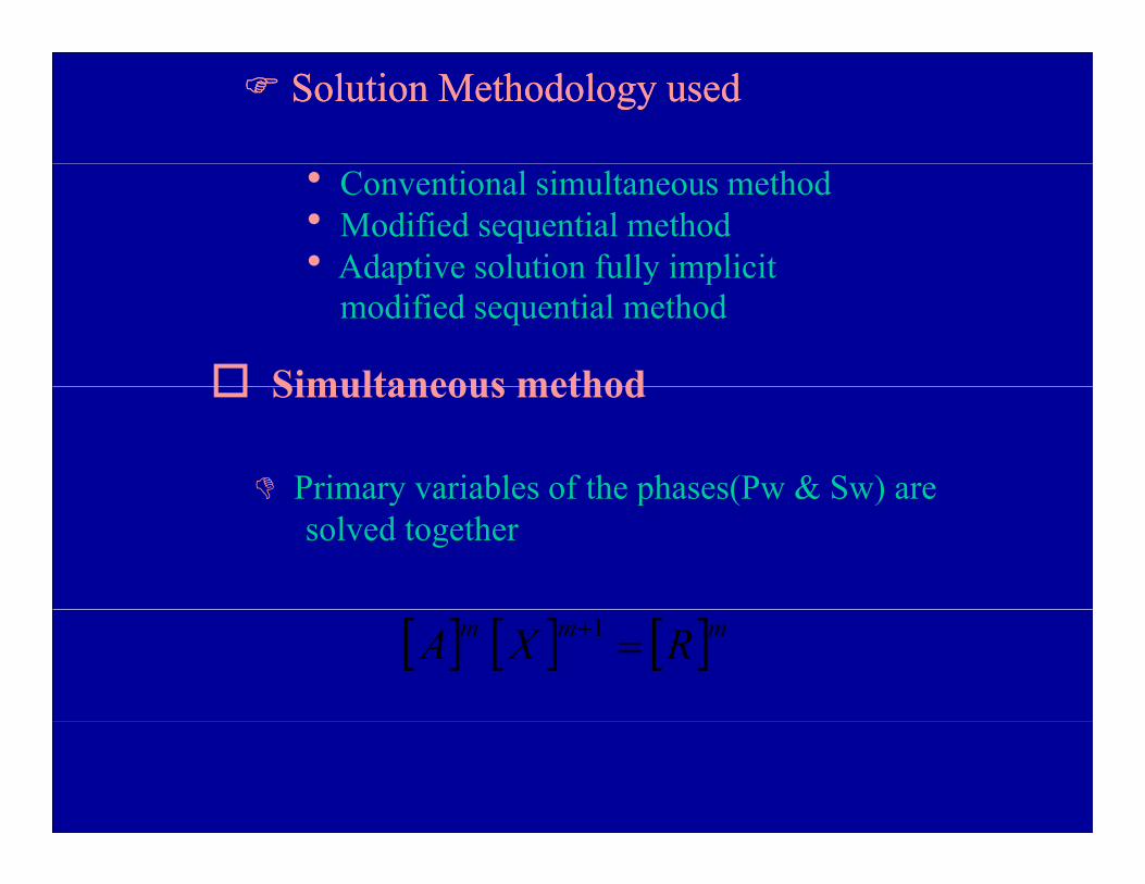
Solution Methodology usedSolution Methodology used
h Conventional simultaneous methodhModified sequential methodhAdaptive solution fully implicitAdaptive solution fully implicit
modified sequential method
Simultaneous method
Primary variables of the phases(Pw & Sw) are
Simultaneous method
Primary variables of the phases(Pw & Sw) aresolved together
[ ] [ ] [ ]mmm RXA =+1
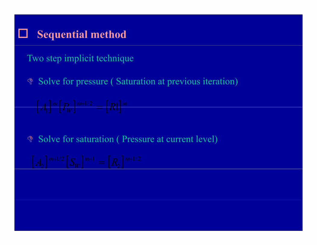
Sequential method
Two step implicit technique
[ ] [ ] [ ]mmm RPA 12/1 =+
Solve for pressure ( Saturation at previous iteration)
[ ] [ ] [ ]W RPA 11 =
Solve for saturation ( Pressure at current level)Solve for saturation ( Pressure at current level)
[ ] [ ] [ ] 2/12
12/12
+++ = mmW
m RSA
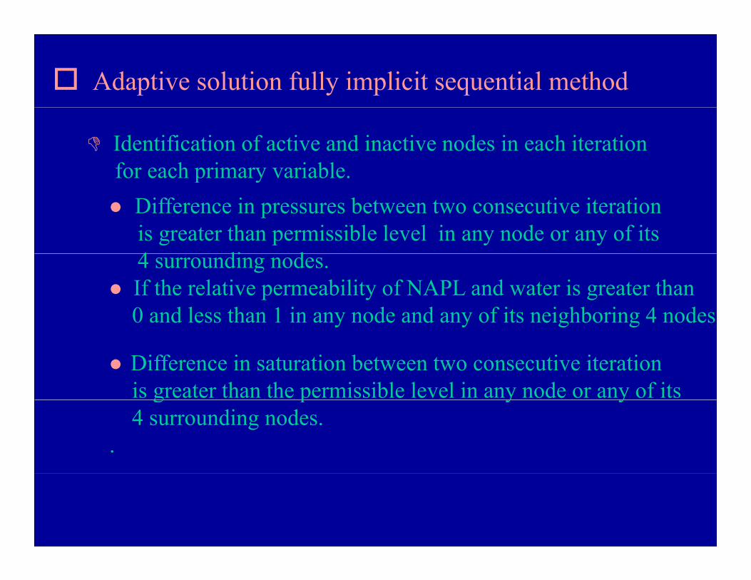
Adaptive solution fully implicit sequential method
Identification of active and inactive nodes in each iterationfor each primary variable.p y
Difference in pressures between two consecutive iterationis greater than permissible level in any node or any of its 4 di d4 surrounding nodes.If the relative permeability of NAPL and water is greater than 0 and less than 1 in any node and any of its neighboring 4 nodesy y g g
Difference in saturation between two consecutive iterationis greater than the permissible level in any node or any of its g p y y4 surrounding nodes.
.

T difi d i l h d
For active nodesFor active nodesTwo step modified sequential method
Solve for pressure ( Saturation at previous iteration) p ( p )
[ ] [ ] [ ]mmW
m RPA 12/1
1 =+
Solve for saturation ( Pressure at current level)[ ] [ ] [ ] 2/1
212/1
2+++ = mm
Wm RSA[ ] [ ] [ ]22 W
For inactive nodesFor inactive nodesPressure and saturation from the previous iteration
Porosity of the medium [m2] 0 35
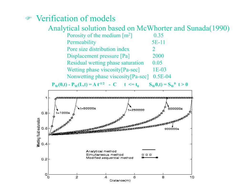
Verification of modelsAnalytical solution based on McWhorter and Sunada(1990)
Porosity of the medium [m ] 0.35Permeability 5E-11Pore size distribution index 2Displacement pressure [Pa] 2000Residual wetting phase saturation 0.05Wetting phase viscosity[Pa-sec] 1E-03Nonwetting phase viscosity[Pa-sec] 0.5E-04
P (0 t) - P (L t) = A t-1/2 - C t <= t S 0 t) = S 0 t > 0PW(0,t) - PW(L,t) = A t - C t <= t0 SW0,t) = SW t > 0
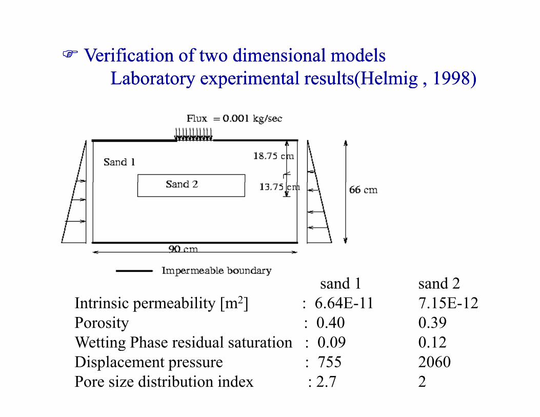
Verification of two dimensional modelsLaboratory experimental results(Helmig 1998)
Verification of two dimensional modelsLaboratory experimental results(Helmig 1998)Laboratory experimental results(Helmig , 1998)Laboratory experimental results(Helmig , 1998)
sand 1 sand 2sand 1 sand 2Intrinsic permeability [m2] : 6.64E-11 7.15E-12Porosity : 0.40 0.39Wetting Phase resid al sat ration : 0 09 0 12Wetting Phase residual saturation : 0.09 0.12Displacement pressure : 755 2060Pore size distribution index : 2.7 2

NAPL saturation distribution at different times
Experimental resultT = 1000sec
T 3000 T = 5000secPresent Model resultsT = 3000sec T = 5000sec

Comparison of different types of models
Between modelsBetween numerical methods
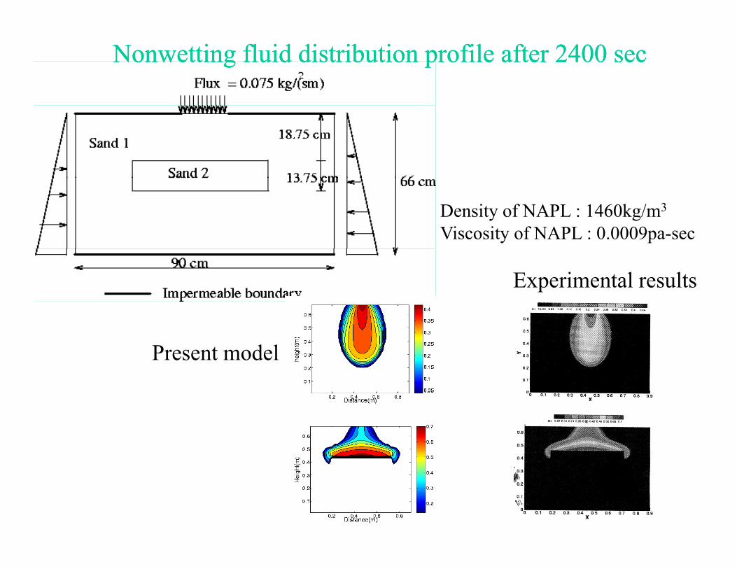
Nonwetting fluid distribution profile after 2400 secNonwetting fluid distribution profile after 2400 sec
Density of NAPL : 1460kg/m3
Viscosity of NAPL : 0.0009pa-sec
Experimental results
Present model
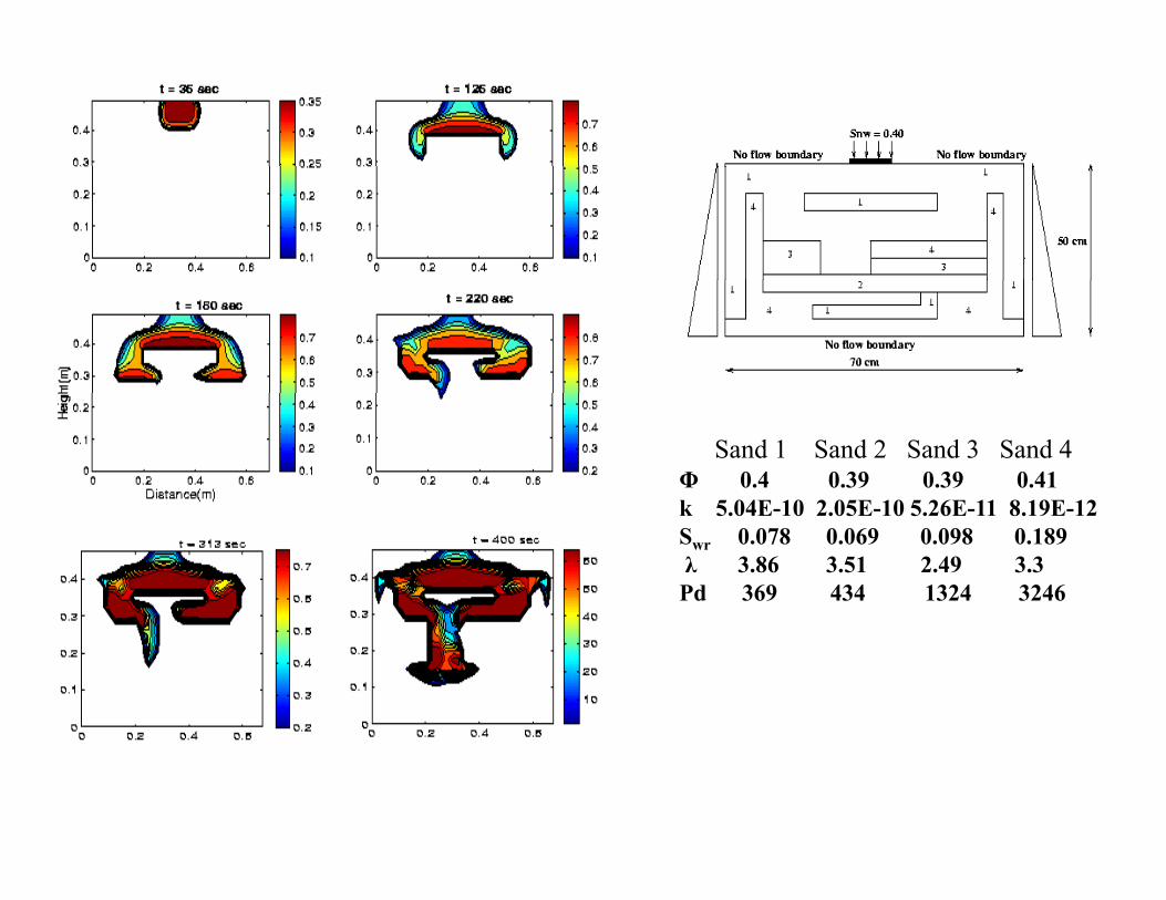
Sand 1 Sand 2 Sand 3 Sand 4Φ 0.4 0.39 0.39 0.41k 5 04E 10 2 05E 10 5 26E 11 8 19E 12k 5.04E-10 2.05E-10 5.26E-11 8.19E-12 Swr 0.078 0.069 0.098 0.189λ 3.86 3.51 2.49 3.3Pd 369 434 1324 3246

Sensitivity study for SIM, MSEM and ASMSEM
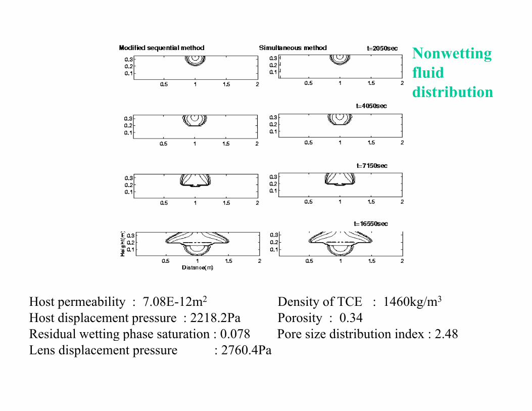
Nonwetting fluidfluid distribution
Host permeability : 7.08E-12m2 Density of TCE : 1460kg/m3
Host displacement pressure : 2218.2Pa Porosity : 0.34Residual wetting phase saturation : 0 078 Pore size distribution index : 2 48Residual wetting phase saturation : 0.078 Pore size distribution index : 2.48Lens displacement pressure : 2760.4Pa
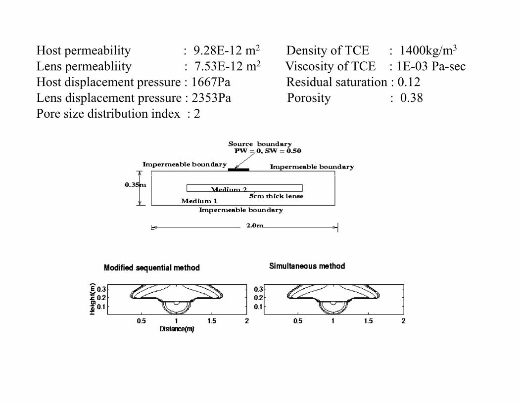
Host permeability : 9.28E-12 m2 Density of TCE : 1400kg/m3
Lens permeabliity : 7.53E-12 m2 Viscosity of TCE : 1E-03 Pa-secHost displacement pressure : 1667Pa Residual saturation : 0.12Lens displacement pressure : 2353Pa Porosity : 0.38Pore size distribution index : 2

Sand 1 Sand 2k 6.64E-11 7.15E-12Φ 0.4 0.39SWr 0.09 0.12SWr 0.09 0.12Pd 755 2060λ 2.7 2ρ 1460kg/m3ρNW 1460kg/m3
μNW 0.9e-03pa-s

Effect of different types of approximations at the cell facesa Arithmetic mean or Harmonic meana Arithmetic mean or Harmonic meanb Harmonic mean with upstream weighing of relative
permeabilitiesc Harmonic mean with upstream weighing of relativec Harmonic mean with upstream weighing of relative
permeability and capillarity diffusivitiesd. Fully upwind method
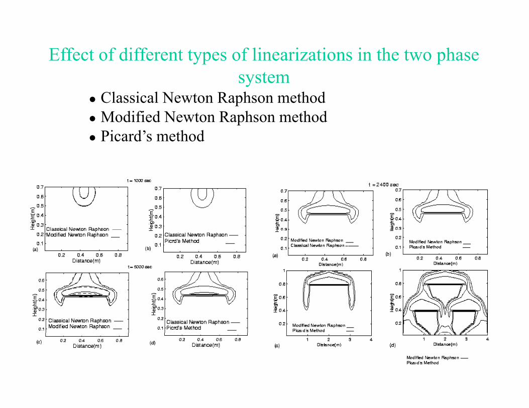
Effect of different types of linearizations in the two phase systemsystem
Classical Newton Raphson methodModified Newton Raphson methodPicard’s method

Effect of classical Newton Raphson method

Influence of capillarity and heterogeneity in Influence of capillarity and heterogeneity in
* P+
two phase simulation two phase simulation
[ ] )(
)(
2/1
*
WLC
e
e
SJP
PPsJ
φσ=
= −
Pc
[ ] )( WLC SJk
P σ
+-
S*
Pd-
Pd+
Wetting fluid saturation0 1Wetting fluid saturation0 1

Effect of without and with heterogeneity and capillary pressure effect
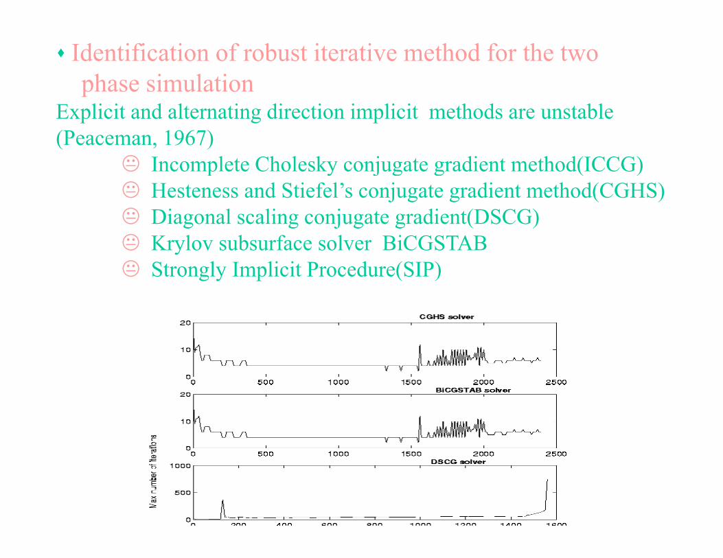
Identification of robust iterative method for the twophase simulation
Explicit and alternating direction implicit methods are unstable(Peaceman, 1967)
Incomplete Cholesky conjugate gradient method(ICCG)p y j g g ( )Hesteness and Stiefel’s conjugate gradient method(CGHS)Diagonal scaling conjugate gradient(DSCG)Krylov subsurface solver BiCGSTABKrylov subsurface solver BiCGSTABStrongly Implicit Procedure(SIP)
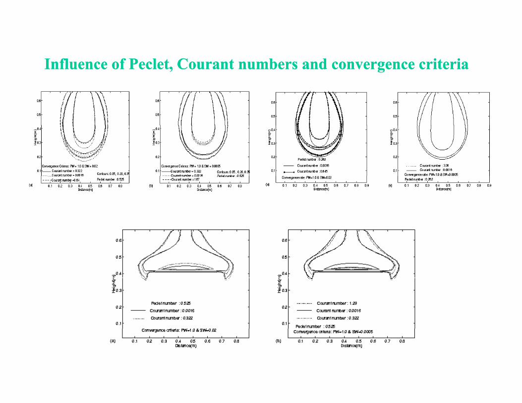
Influence of Peclet, Courant numbers and convergence criteriaInfluence of Peclet, Courant numbers and convergence criteria
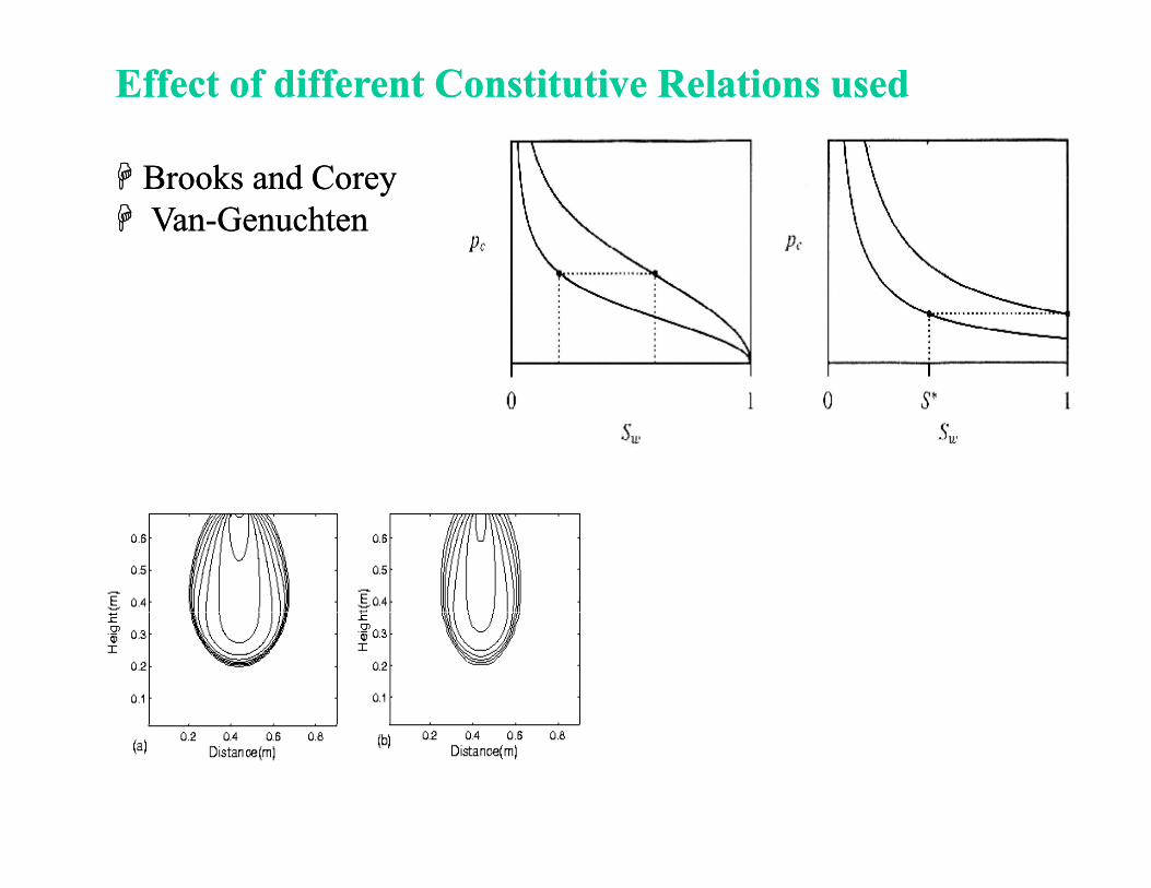
Effect of different Constitutive Relations usedEffect of different Constitutive Relations used
Brooks and CoreyVan-GenuchtenBrooks and CoreyVan-Genuchten

Effect of NAPL migration in Random Heterogeneous Media
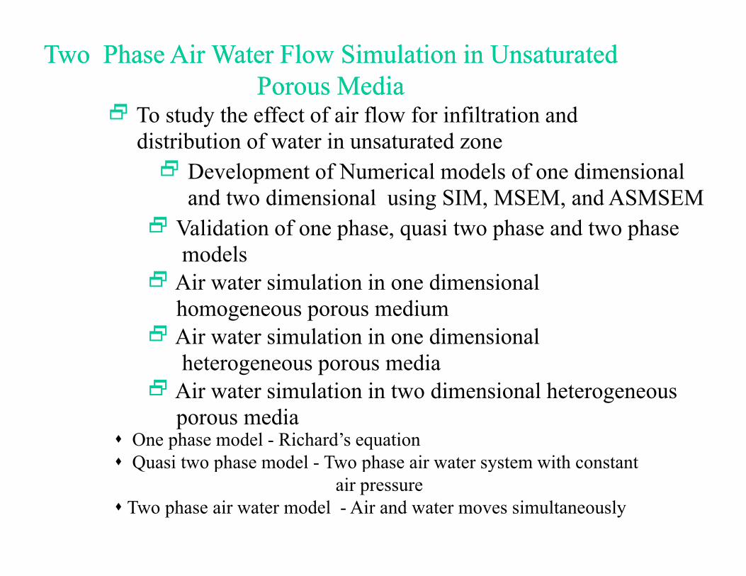
Two Phase Air Water Flow Simulation in UnsaturatedPorous Media
Two Phase Air Water Flow Simulation in UnsaturatedPorous Media
2 d h ff f i fl f i fil i d
2 Development of Numerical models of one dimensional
2 To study the effect of air flow for infiltration and distribution of water in unsaturated zone
pand two dimensional using SIM, MSEM, and ASMSEM
2 Validation of one phase, quasi two phase and two phasemodelsmodels
2Air water simulation in one dimensional homogeneous porous medium
2Air water simulation in one dimensional heterogeneous porous media
2Air water simulation in two dimensional heterogeneousAir water simulation in two dimensional heterogeneous porous media
One phase model - Richard’s equationQuasi two phase model - Two phase air water system with constant Q p p y
air pressureTwo phase air water model - Air and water moves simultaneously

One phase model - Richard’s equationVerification of quasi two phase model using one phase modelVerification of quasi two phase model using one phase model
p qQuasi two phase model - Arithmetic approximation
- Harmonic approximation with upstream nodal relative
Flux = 3.29m/day i i l
upstream nodal relative permeabilities
Initial pressure = -0.615m

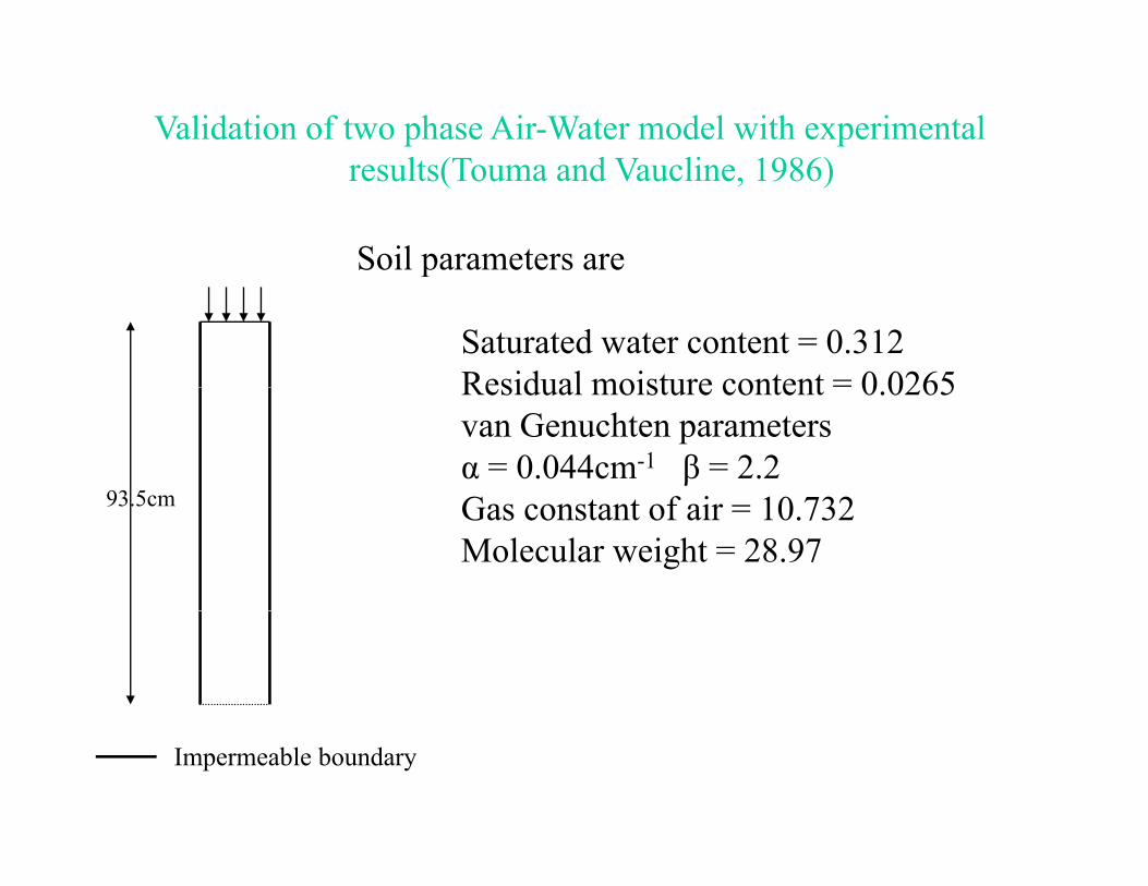
Validation of two phase Air-Water model with experimentallt (T d V li 1986)results(Touma and Vaucline, 1986)
Soil parameters arep
Saturated water content = 0.312Residual moisture content = 0 0265
93 5cm
Residual moisture content 0.0265van Genuchten parametersα = 0.044cm-1 β = 2.2G f i 10 73293.5cm Gas constant of air = 10.732Molecular weight = 28.97
Impermeable boundary

Flux greater than hydraulic conductivity - 20cm/h
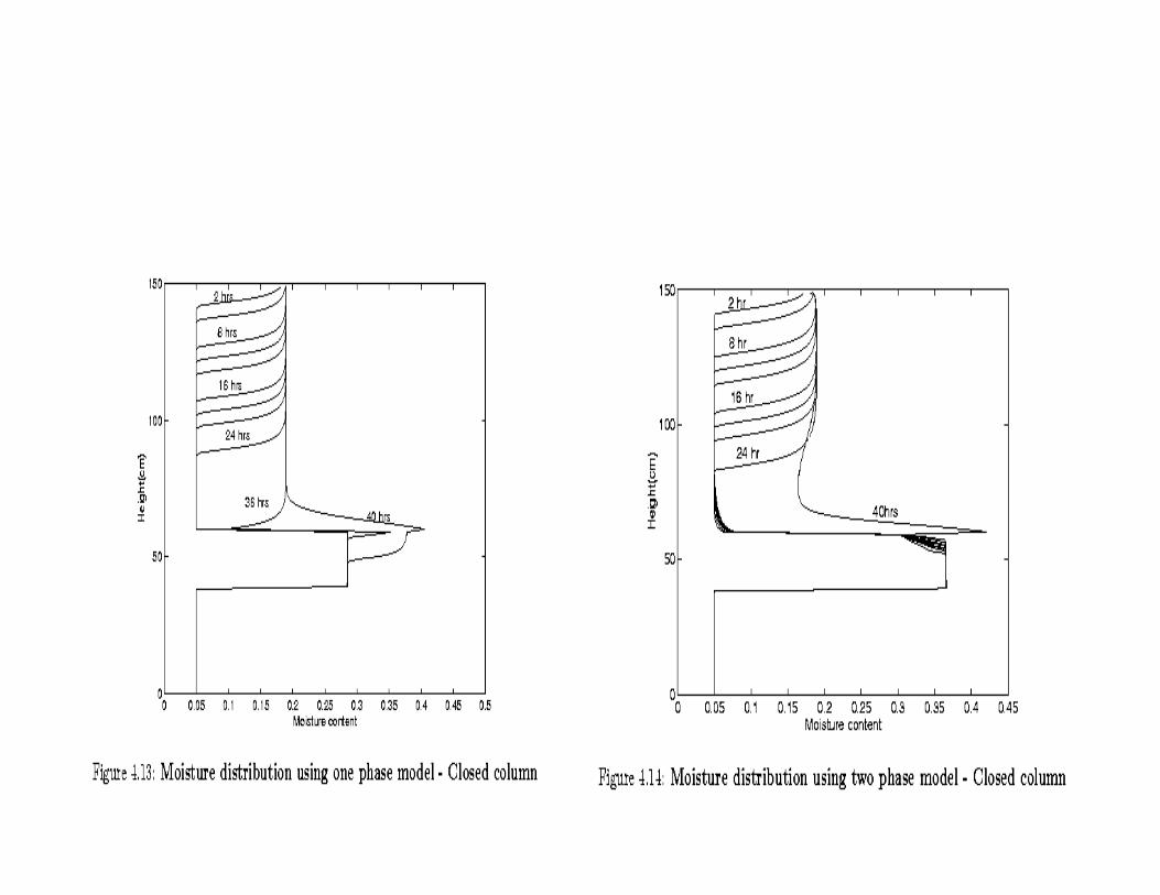
Bounded column
Two phase model One phase model
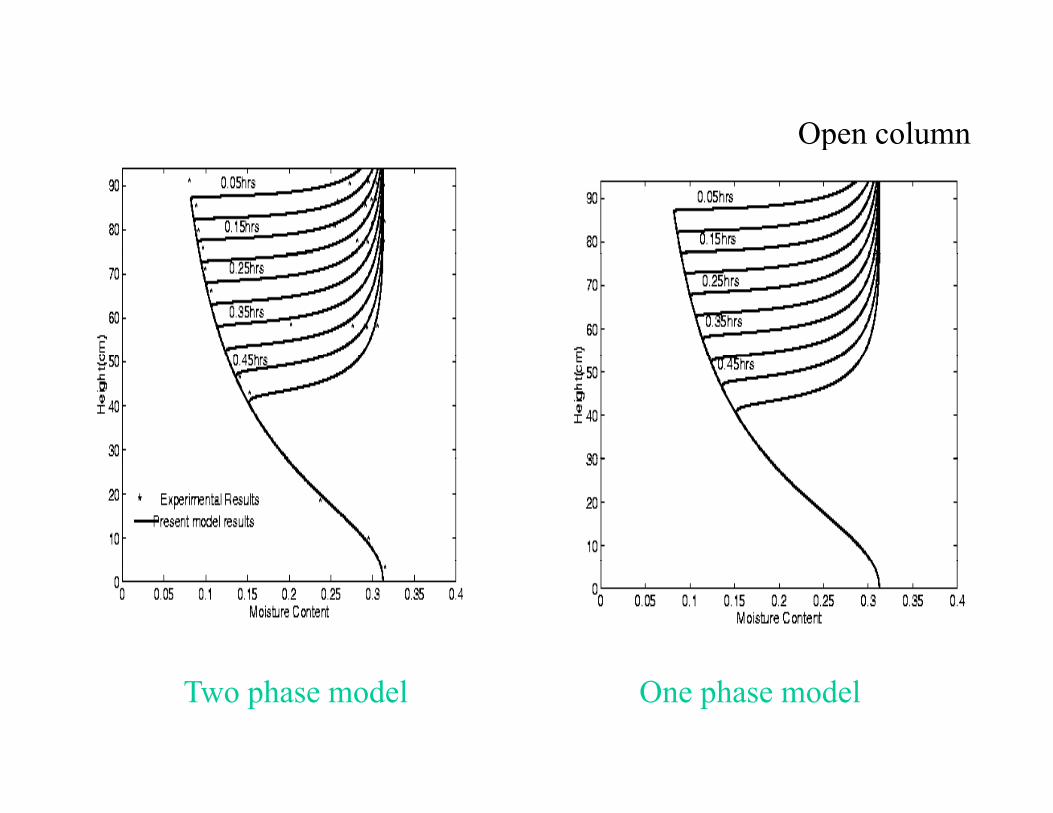
Open columnp
Two phase model One phase model
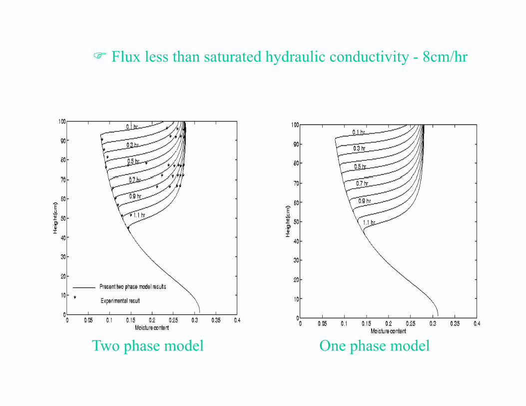
Flux less than saturated hydraulic conductivity - 8cm/hr
Two phase model One phase model
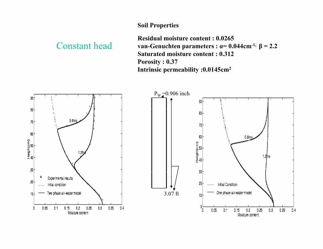
Constant head
Soil Properties
Residual moisture content : 0.0265van Genuchten parameters : α= 0 044cm-1, β = 2 2Constant head van-Genuchten parameters : α= 0.044cm 1, β = 2.2Saturated moisture content : 0.312Porosity : 0.37Intrinsic permeability :0.0145cm2
PW =0.906 inch
3.07 ft
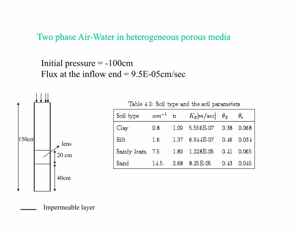
Two phase Air-Water in heterogeneous porous mediaTwo phase Air-Water in heterogeneous porous media
Initial pressure = -100cmFl t th i fl d 9 5E 05 /Flux at the inflow end = 9.5E-05cm/sec
150cm
20 cm
lens
40cm
Impermeable layer
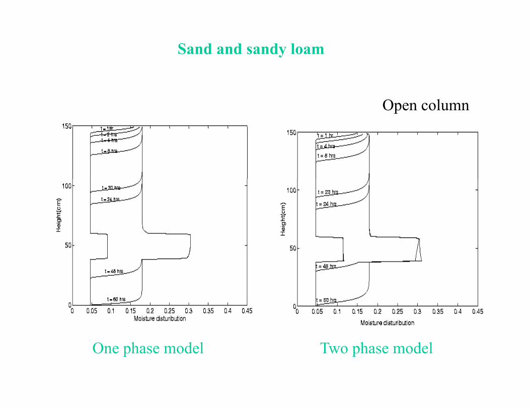
Sand and sandy loam
Open column
One phase model Two phase model
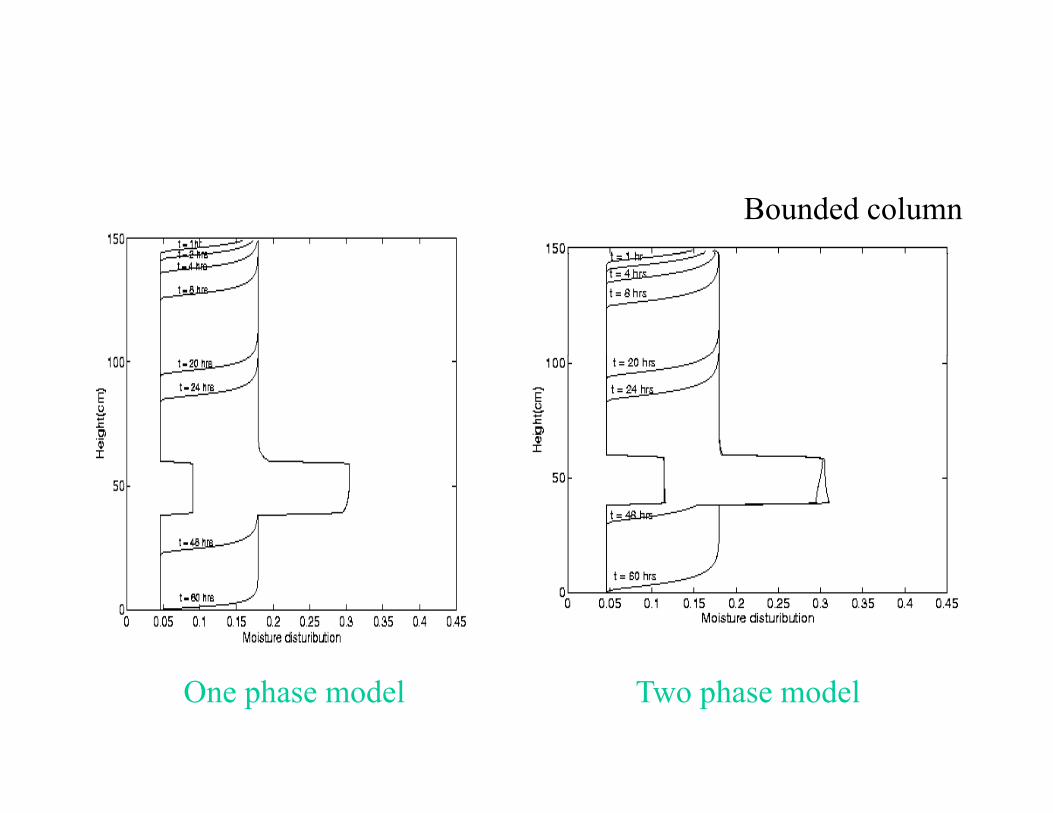
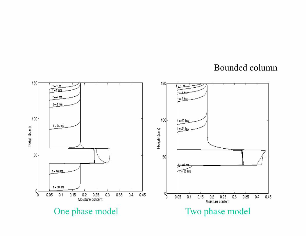
Bounded column
One phase model Two phase model

Sand and Silt
Open column
One phase model Two phase model
Bounded column
One phase model Two phase model

Sand and Clay

Two dimensional two phase air water simulation in heterogeneous media
Two dimensional two phase air water simulation in heterogeneous media
Fl 1 13 10 5 / Initial pressure = -150cm10cm
sand
Flux = 1.13x10⁻⁵ cm/sec
20
15cm50cm
60
Low permeability soil
20cm
100 cm
60cm
Test One phase Two phase Two phase Two phaseproblem model MSEM SIM ASMSEM
1 1217 1893 2272 7992 1229 1952 2389 822

Sand and Sandy loam

Modelling and Simulation of NAPL Migration in Saturated -unsaturated zone
Modelling and Simulation of NAPL Migration in Saturated -unsaturated zoneu s u ed o eu s u ed o e
2 Development of three phase model of water, NAPL, and air2 Q i th h d l Ai NAPL W t2 Quasi three phase model - Air - NAPL - Water
with static air pressure2 Fully three phase model - Air- NAPL - Water
with air pressure 2 Validation of the present models
2 Effect of capillary pressure and heterogeneityin the numerical modelling of three phase systems
2 Comparative study between simultaneous, sequential and adaptivemodified sequential methods for the saturated unsaturated systems
2 Effect of air pressure on the numerical modelling of three phasesystems

Model ValidationModel Validation
Oil infiltration
15 cm3 cm
30 cm
20 cm
Watertable
Infiltration : 30ml of NAPL , 20,5,5----1hr interval -----case a: 30ml ------30ml for 3hrs-----------case b
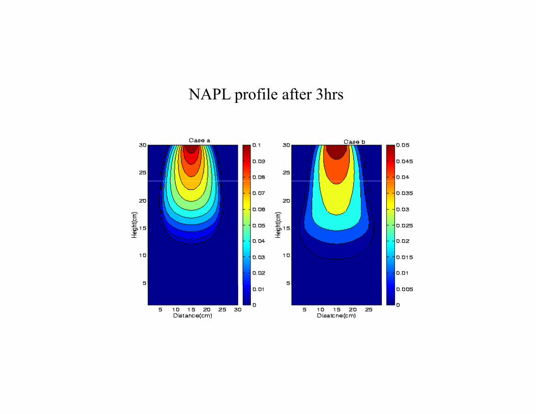
NAPL profile after 3hrs


Air-NAPL-Water simulation in variably saturated mediay
Infiltartion rate- 5.07E-05m/sec

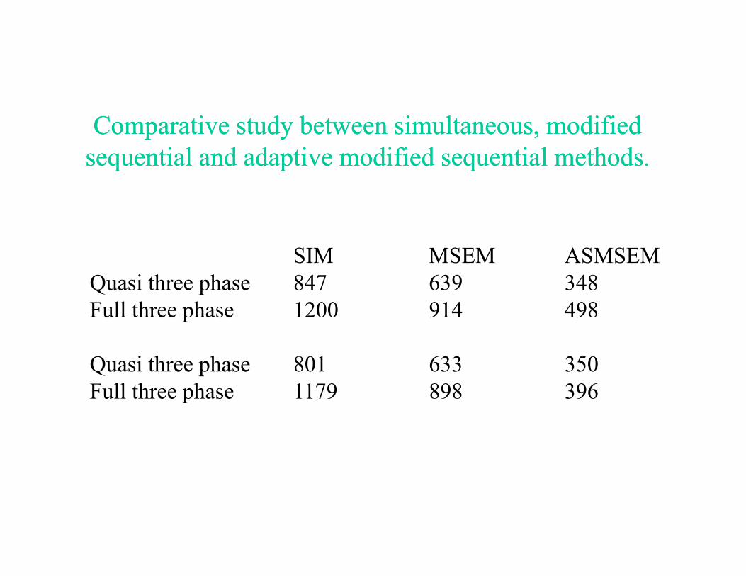
Comparative study between simultaneous, modified sequential and adaptive modified sequential methods.Comparative study between simultaneous, modified
sequential and adaptive modified sequential methods.
SIM MSEM ASMSEMSIM MSEM ASMSEMQuasi three phase 847 639 348Full three phase 1200 914 498
Quasi three phase 801 633 350Full three phase 1179 898 396Full three phase 1179 898 396

Effect of capillarity and heterogeneity in the numerical p y g ymodelling of three phase systems
LNAPL
Flux = 7.1x10⁻⁴m/sec
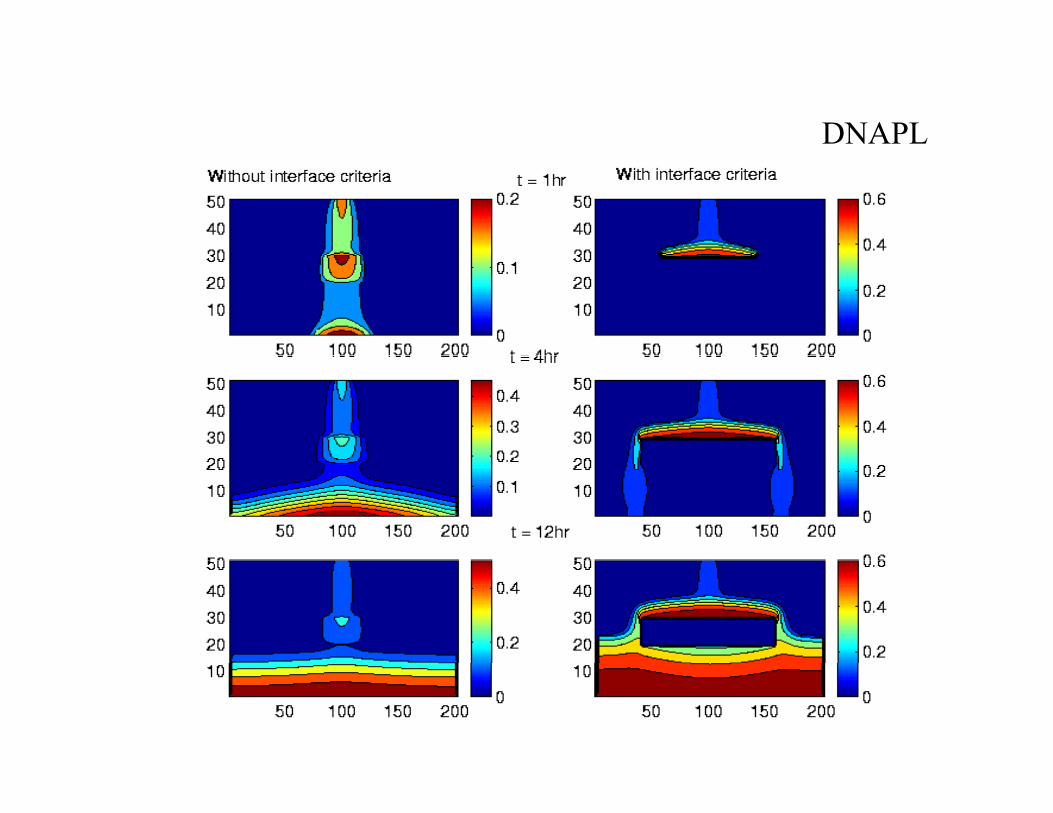
DNAPL
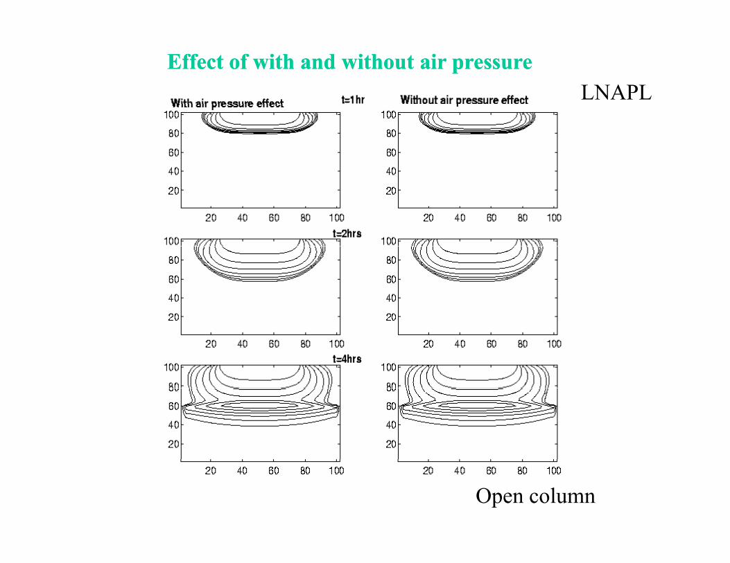
Effect of with and without air pressureEffect of with and without air pressureLNAPL
Open column
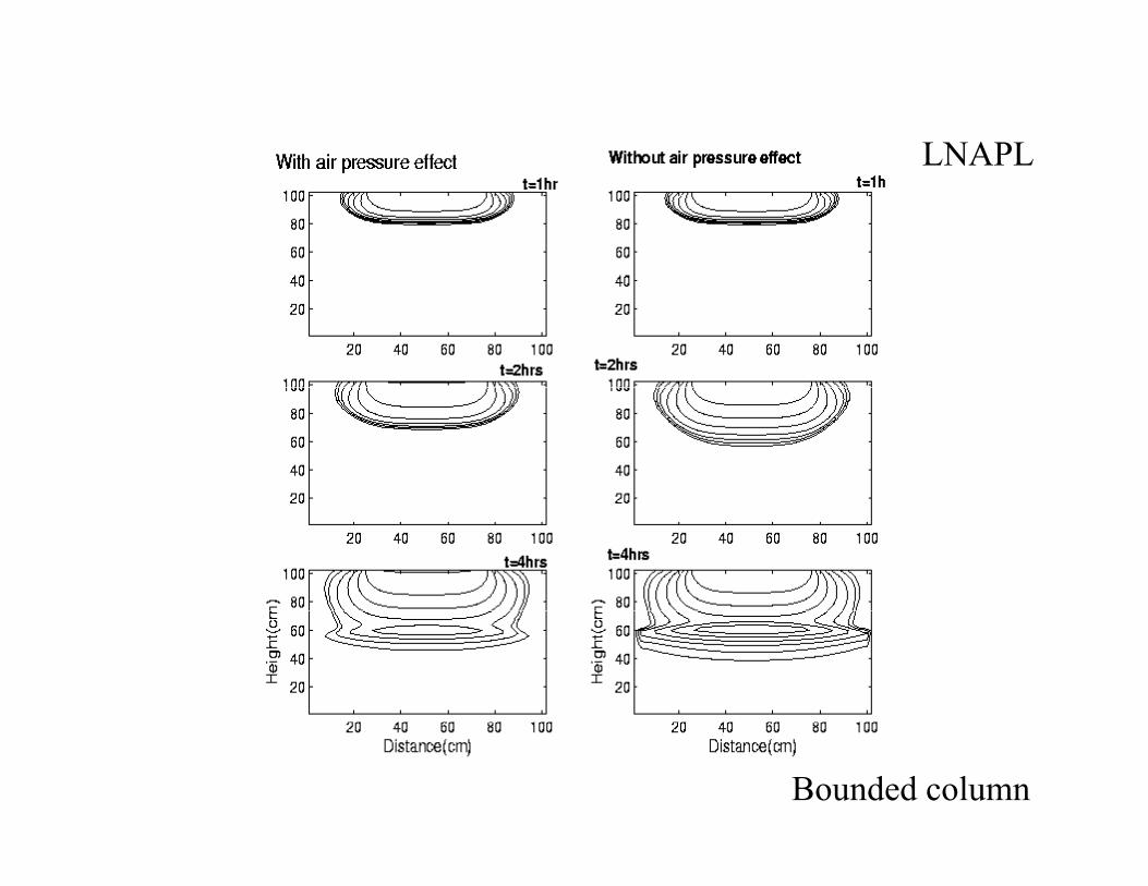
LNAPLLNAPL
Bounded column
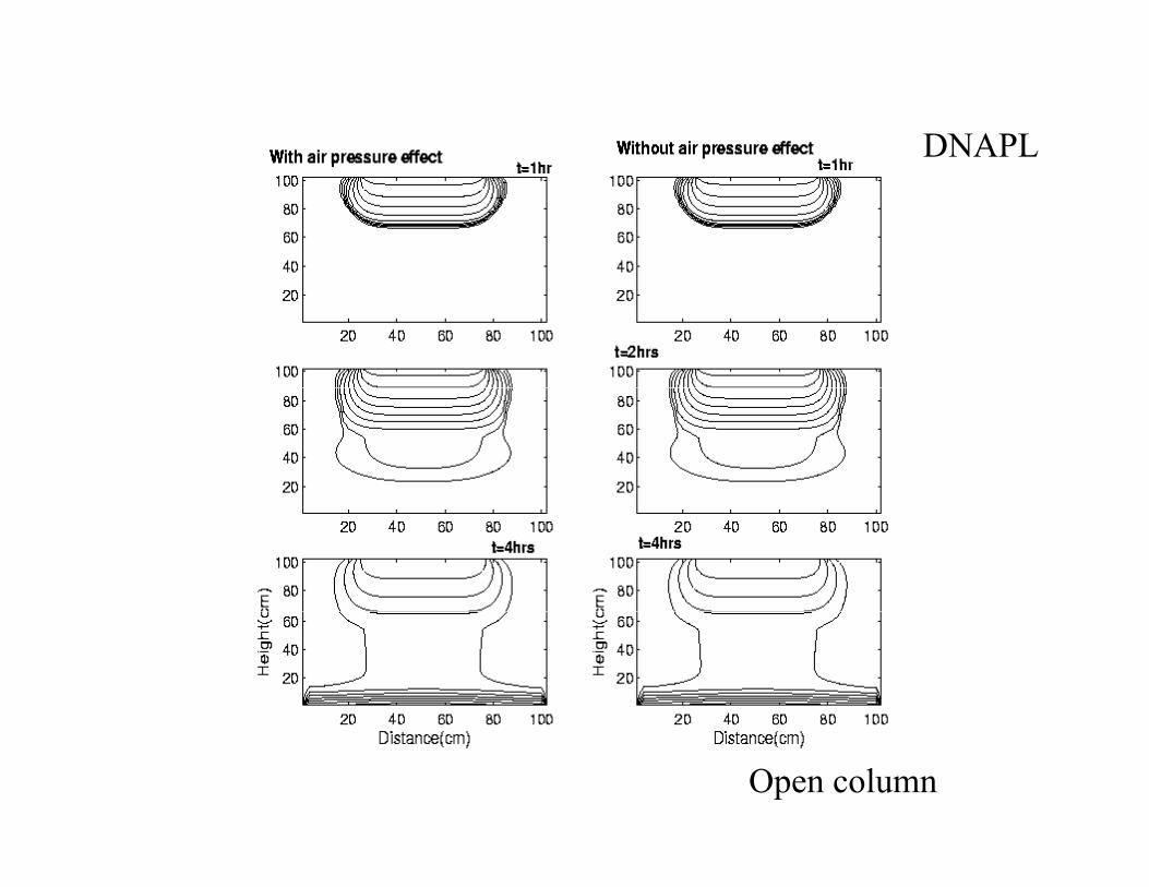
DNAPL
Open column

DNAPL
Bounded column
Parallel computation of NAPL migartion in saturated porous media
Parallel computation of NAPL migartion in saturated porous mediapp
Need of Parallel ComputationTo reduce the computational timeTo reduce the computational time
To simulate bigger domain multiphase flow simulations which is not possible by conventional computation
General Parallel Architecture - Interaction between the processorsGeneral Parallel Architecture Interaction between the processors
Shared memory programmingy p g g
Distributed memory with Message Passing Interface programmingprogramming
Data parallel programming
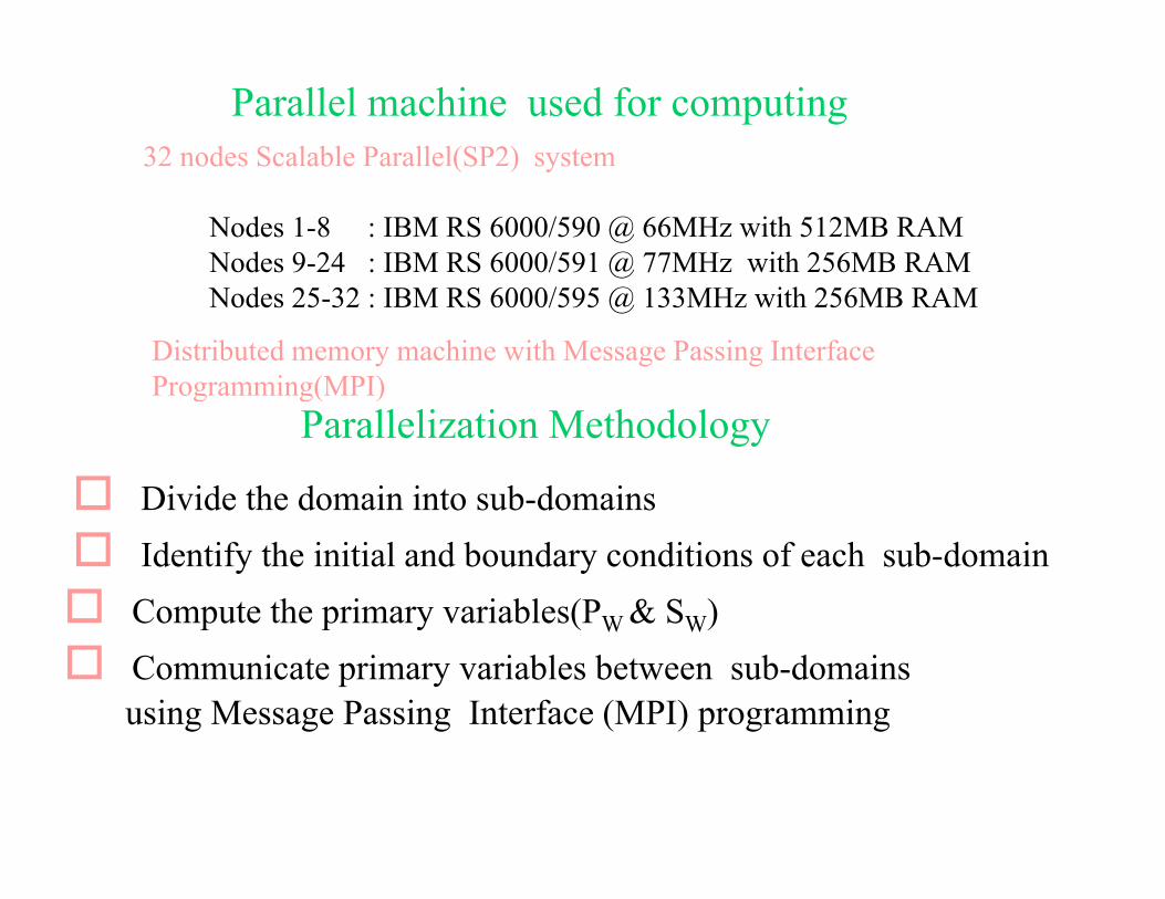
Parallel machine used for computing32 nodes Scalable Parallel(SP2) system3 odes Sca ab e a a e (S ) sys e
Nodes 1-8 : IBM RS 6000/590 @ 66MHz with 512MB RAMNodes 9-24 : IBM RS 6000/591 @ 77MHz with 256MB RAMNodes 25-32 : IBM RS 6000/595 @ 133MHz with 256MB RAM
Distributed memory machine with Message Passing InterfaceProgramming(MPI)Programming(MPI)
Divide the domain into sub-domains
Parallelization Methodology
Divide the domain into sub domainsIdentify the initial and boundary conditions of each sub-domainCompute the primary variables(PW & SW)Compute the primary variables(PW & SW)Communicate primary variables between sub-domains using Message Passing Interface (MPI) programming

Domain Decomposition methods usedDomain Decomposition methods used
1 1
2
3
Overlapping region 2
3
Row wise Column wise
3
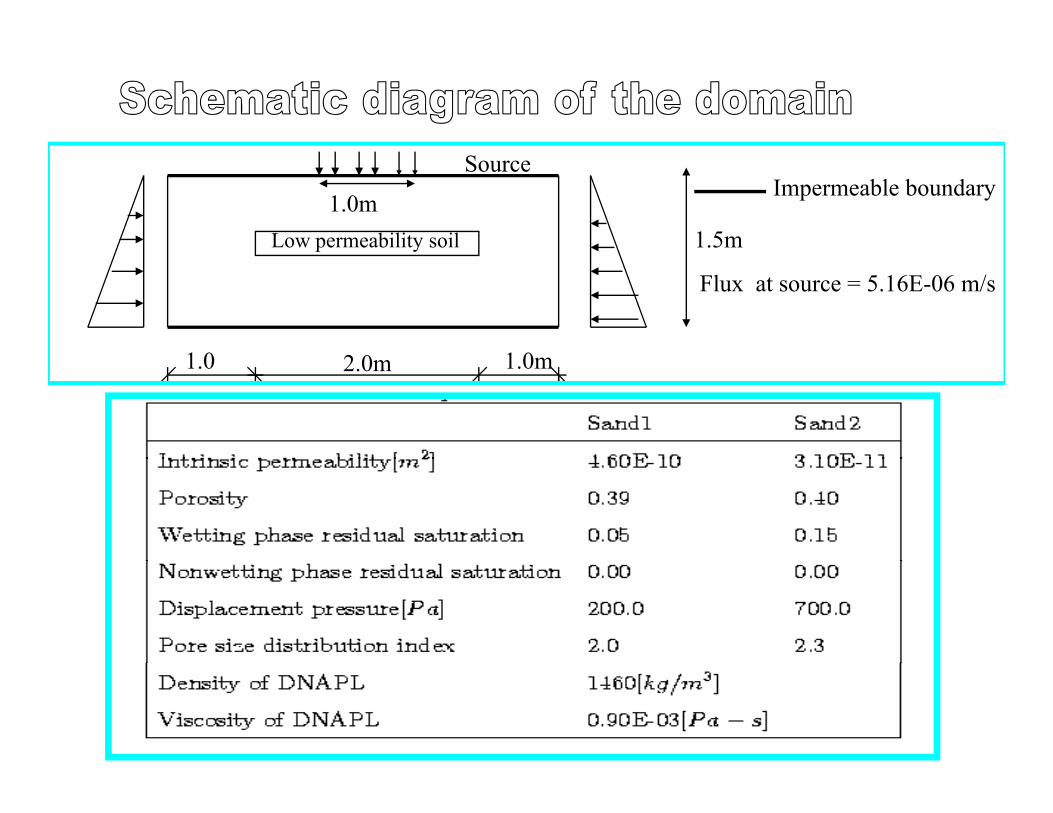
Source
1.5m
Impermeable boundary1.0m
Low permeability soil
1 0 1 02 0
Flux at source = 5.16E-06 m/s
1.0 1.0m2.0m


Properties Sand 1 Sand 2
Properties of media and fluidProperties Sand 1 Sand 2
Porosity 0.40 0.41Displacement pressure[Pa] 369 3246
2Intrinsic permeability [m2] 5.04E-11 8.19E-12Residual saturation 0.078 0.1189pore size distribution index 3.86 3.3
Density of NAPL[kg/m3] 1460Viscosity[Pa-s ] 0.90E-03

Nonwetting fluid saturation distributionNonwetting fluid saturation distribution
after 1day after 3days
Modelling of Multiphase Flow in a Fracture Mediaa Fracture Media
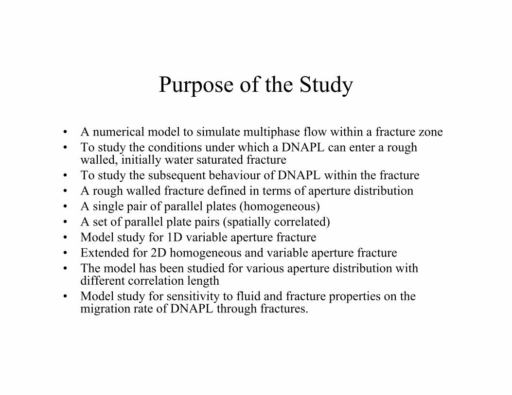
Purpose of the Study
• A numerical model to simulate multiphase flow within a fracture zone• To study the conditions under which a DNAPL can enter a rough
walled, initially water saturated fracture T t d th b t b h i f DNAPL ithi th f t• To study the subsequent behaviour of DNAPL within the fracture
• A rough walled fracture defined in terms of aperture distribution• A single pair of parallel plates (homogeneous)• A set of parallel plate pairs (spatially correlated)• A set of parallel plate pairs (spatially correlated)• Model study for 1D variable aperture fracture• Extended for 2D homogeneous and variable aperture fracture• The model has been studied for various aperture distribution with e ode as bee s ud ed o va ous ape u e d s bu o w
different correlation length• Model study for sensitivity to fluid and fracture properties on the
migration rate of DNAPL through fractures.
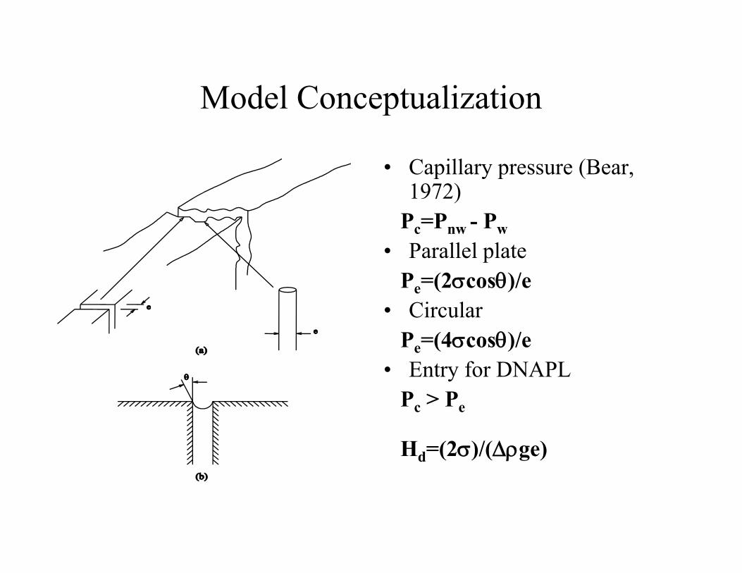
Model ConceptualizationModel Conceptualization
• Capillary pressure (Bear, p y p (1972)
Pc=Pnw - Pw• Parallel plate• Parallel plate
Pe=(2σcosθ)/e• Circular
Pe=(4σcosθ)/e• Entry for DNAPL
P > PPc > Pe
Hd=(2σ)/(Δρge)

Height of Pool versus Aperture Invaded10
2
( μ
m )
σ = 0.045 N/m
σ = 0.035 N/m
101
ER
TU
RE
INV
AD
ED
( σ = 0.025 N/m
σ = 0.015 N/m
σ = 005 N/m
100
FR
AC
TU
RE
AP
E
10−2
10−1
100
101
102
103
10−1
HEIGHT OF DNAPL POOL (m)

Mathematical Equations
• Mass conservation- ∂(ρw qwi e)⁄∂xi = (∂(φ Sw ρw)/t) e
- ∂(ρnw qnwi e)⁄∂xi = (∂(φ Snw ρnw)⁄∂t)e
• Darcy’s law(k k / ) (∂P /∂ + ∂ /∂ )qwi= - (kijkrw/μw) (∂Pw/∂xj+ρwg∂y/∂xj)
qnwi= - (kijkrnw/μnw) (∂Pnw/∂xj+ρnwg∂y/∂xj)
• Continuity equations(∂/∂xi)[(ekijkrw/μw)(∂Pw/∂xj + (ρwg) (∂y/∂xj))] = eφ(∂Sw/∂t)
(∂/∂xi)[(ekijkrnw/μnw)(∂Pnw/∂xj + (ρnwg) (∂y/∂xj))] = eφ(∂Snw/∂t)
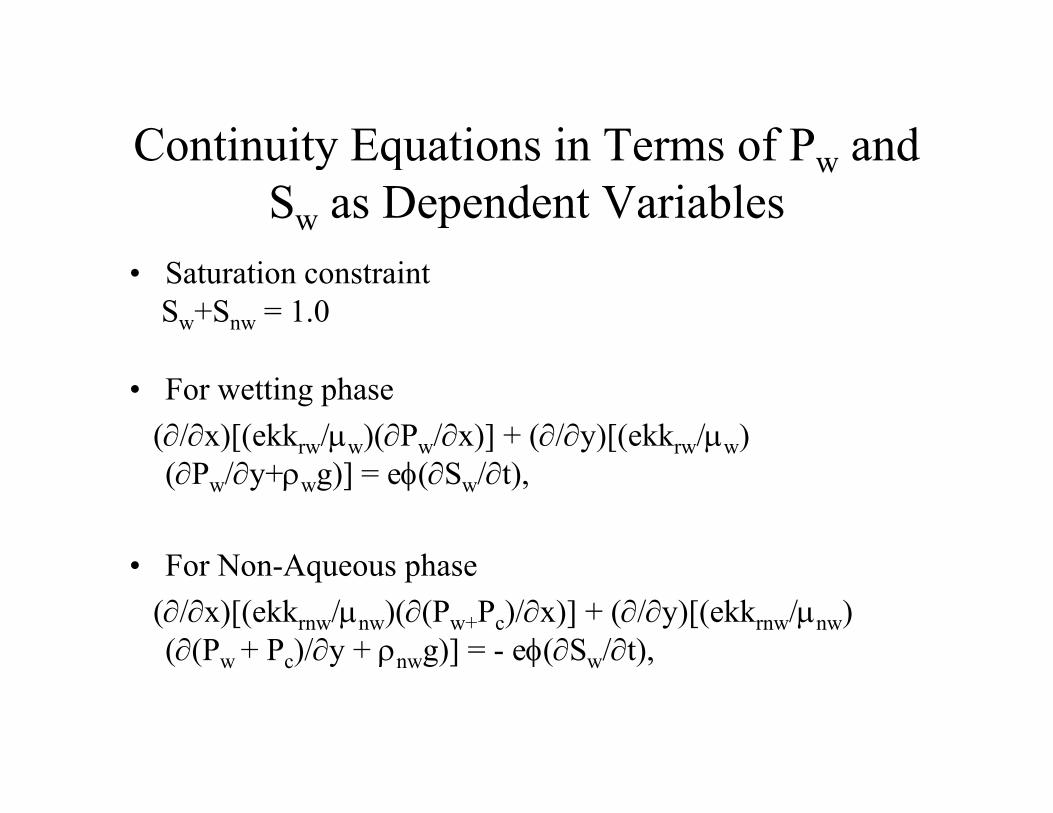
Continuity Equations in Terms of P andContinuity Equations in Terms of Pw and Sw as Dependent Variables
• Saturation constraintSw+Snw = 1.0
• For wetting phase(∂/∂x)[(ekkrw/μw)(∂Pw/∂x)] + (∂/∂y)[(ekkrw/μw) (∂Pw/∂y+ρwg)] = eφ(∂Sw/∂t),
F N A h• For Non-Aqueous phase(∂/∂x)[(ekkrnw/μnw)(∂(Pw+Pc)/∂x)] + (∂/∂y)[(ekkrnw/μnw) (∂(Pw + Pc)/∂y + ρnwg)] = - eφ(∂Sw/∂t),( ( w c) y ρnwg)] φ( w ),

B d C ditiBoundary ConditionsNeumann boundary with zero flux
Constant mass flow rate or constant pressure-saturation
Dirichlet boundary Dirichlet boundary
Neumann boundary with zero flux
a) Dirichlet boundary condition: u1 = f1 and u2 = f2
b) Neumann boundary condition:
(k k /μ ) (∂P /∂x +ρ g∂y/∂x ) = f- (kijkrw/μw) (∂Pw/∂xj+ρwg∂y/∂xj) = f3- (kijkrnw/μnw) (∂Pnw/∂xj+ρnwg∂y/∂xj) = f4
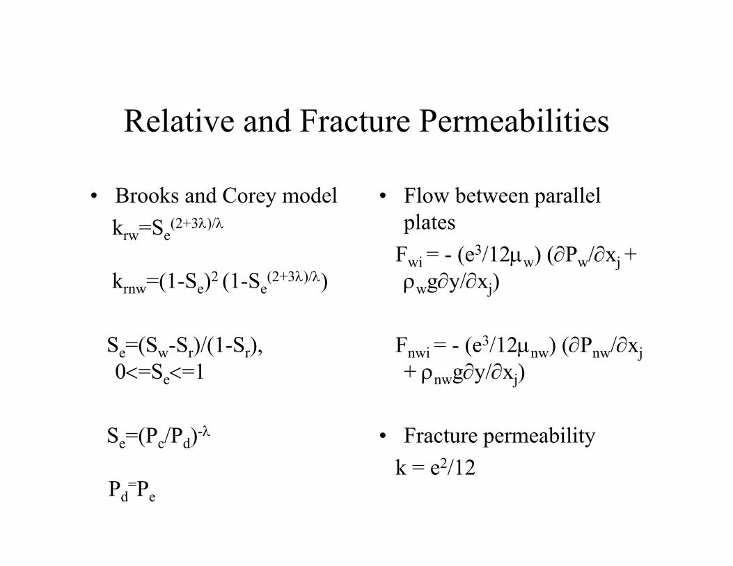
Relative and Fracture Permeabilities
• Brooks and Corey modelkrw=Se
(2+3λ)/λ
• Flow between parallel plates
F ( 3/12 ) (∂P /∂krnw=(1-Se)2 (1-Se
(2+3λ)/λ)Fwi = - (e3/12μw) (∂Pw/∂xj + ρwg∂y/∂xj)
Se=(Sw-Sr)/(1-Sr), 0<=Se<=1
Fnwi = - (e3/12μnw) (∂Pnw/∂xj + ρnwg∂y/∂xj)
Se=(Pc/Pd)-λ • Fracture permeabilityk 2/12
Pd=Pe
k = e2/12
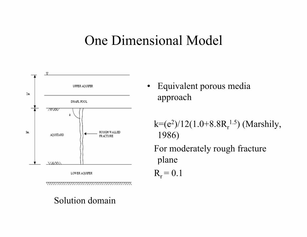
One Dimensional ModelOne Dimensional Model
• Equivalent porous media approach
k=(e2)/12(1.0+8.8Rr1.5) (Marshily,
1986)1986)For moderately rough fracture plane p
Rr = 0.1
Solution domain

Fluid and Fracture PropertiesFluid and Fracture Properties
Properties Values Units
Wetting phase viscosity 0.001 Pa.s
Nonwetting phase viscosity 0.00057 Pa.s
Wetting phase density 1000.0 Kg/m3
Nonwetting phase density 1460.0 Kg/m3
Interfacial tension 0.045 N/m
Porosity 0.8 -
Pore size distribution index 1.0 -
Wetting phase residual saturation 0.1 -

Model VerificationModel Verification
2
2.5
present model for density = 1460 kg/m3
Kueper’s model for density = 1460 kg/m3
present model for density = 1200 kg/m3
Kueper’s model for density = 1200 kg/m3
160
180
200
present model for density = 1460 kg/m3
Kueper’s model for density = 1460 kg/m3
present model for density = 1200 kg/m3
Kueper’s model for density = 1200kg/m3
1
1.5
Po
ol H
eig
ht
(met
ers)
60
80
100
120
140
Ap
ertu
re (
mic
ron
s)
Kueper s model for density = 1200kg/m
0 1 2 3 4 5 6 7 8 9 100
0.5
Time (hours)
0 5 10 15 20 25 300
20
40
Time (hours)
DNAPL pool vs time Aperture vs time
60
70
80
90
es)
Kueper’s ResultPresent Model
DNAPL pool vs time Aperture vs time
20
30
40
50
60
Fra
ctu
re D
ip (
deg
ree
0 1 2 3 4 5 60
10
Time (hours)
Fracture dip vs time

Sensitivity with DNAPL Pooled AboveSensitivity with DNAPL Pooled Above Fracture Opening
120
140DNAPL pool height = 0.5 mDNAPL pool height = 1.0 mDNAPL pool height = 1.5 mDNAPL pool height = 2.0 m
0.4
0.45
DNAPL pool = 0.50 mDNAPL pool = 0.40 mDNAPL pool = 0.30 mDNAPL pool = 0 35 m
80
100
per
ture
(m
icro
ns)
0 2
0.25
0.3
0.35
PL
Sat
urat
ion
DNAPL pool = 0.35 m
20
40
60
Fra
ctu
re A
p
0.05
0.1
0.15
0.2
DN
AP
0 2 4 6 8 10 12 14 16 180
Time (hours)
0 0.5 1 1.5 2 2.5 3 3.5 4 4.5 50
0.05
Length of Fracture (m)
F t tFracture aperture vs travel time
DNAPL saturation att = 15000s

Sensitivity with aperture of FractureSensitivity with aperture of Fracture Opening
2.5
3
Fracture Aperture = 100 μmFracture Aperture = 75 μm Fracture Aperture = 50 μm Fracture Aperture = 25 μm 0 4
0.45
0.5
1.5
2
ol H
eig
ht
(met
ers)
Fracture Aperture = 25 μm
0.25
0.3
0.35
0.4
PL
Sat
urat
ion
e = 25 μme = 50 μme = 75 μme = 100 μm
0.5
1
DN
AP
L P
oo
0.1
0.15
0.2DN
AP
0 5 10 15 20 25 30 35 40 45 500
Time (hours)0 0.5 1 1.5 2 2.5 3 3.5 4 4.5 5
0
0.05
Length of Fracture (m)
DNAPL Pool vs travel time DNAPL saturation att = 15000s

Sensitivity With Fracture DipSensitivity With Fracture Dip
0.45
0.5
Dip = 15o Dip = 30o
0.35
0.4Dip = 0o
Dip = 30
Dip = 45o
Dip = 60o
0.25
0.3
AP
L S
atu
ratio
n
Dip = 90o
0 1
0.15
0.2DN
0 0 5 1 1 5 2 2 5 3 3 5 4 4 5 50
0.05
0.1
0 0.5 1 1.5 2 2.5 3 3.5 4 4.5 5Length of Fracture (m)
DNAPL saturation at t = 15000s

Effect of Viscosity and DensityEffect of Viscosity and Density
0.9
1
Fracture Dip = 90 degree
Aperture = 75 μ m
0.9
1
Fracture Dip = 90 degree
Aperture = 75 μ m
0.4
0.5
0.6
0.7
0.8
DN
AP
L S
atu
rati
on
Time = 1000 secondsTime = 2000 secondsTime = 5000 secondsTime = 10000 seconds
Aperture = 75 μ m
DNAPL Pool = 0.5 m
Viscosity = 0.57E−03
0.4
0.5
0.6
0.7
0.8
DN
AP
L S
atu
rati
on
Time = 1000 secondsTime = 2000 secondsTime = 5000 secondsTime = 10000 seconds
DNAPL Pool = 0.5 m
DNAPL Density = 1460 kg/m3
0 0.5 1 1.5 2 2.5 3 3.5 4 4.5 50
0.1
0.2
0.3
Length of Fracture (meters)
0 0.5 1 1.5 2 2.5 3 3.5 4 4.5 50
0.1
0.2
0.3
Length of Fracture (meters)
0.6
0.7
0.8
0.9
1
ura
tio
n
Time = 1000 secondsTime = 2000 secondsTime = 5000 secondsTime = 10000 seconds
Fracture Dip = 90 degree
Aperture = 75 μ m
DNAPL Pool = 0.5 m
Viscosity = 0.9E−03
0.6
0.7
0.8
0.9
1
atu
rati
on
Time = 1000 secondsTime = 2000 secondsTime = 5000 secondsTime = 10000 seconds
Fracture Dip = 90 degree
Aperture = 75 μ m
DNAPL Pool = 0.5 m
DNAPL Density = 1600 kg/m3
0.1
0.2
0.3
0.4
0.5
DN
AP
L S
atu
0.1
0.2
0.3
0.4
0.5
DN
AP
L S
a
0 0.5 1 1.5 2 2.5 3 3.5 4 4.5 50
Length of Fracture (meters)
0 0.5 1 1.5 2 2.5 3 3.5 4 4.5 50
Length of Fracture (meters)
DNAPL saturation plots for viscosity effect
DNAPL saturation plots for density effect
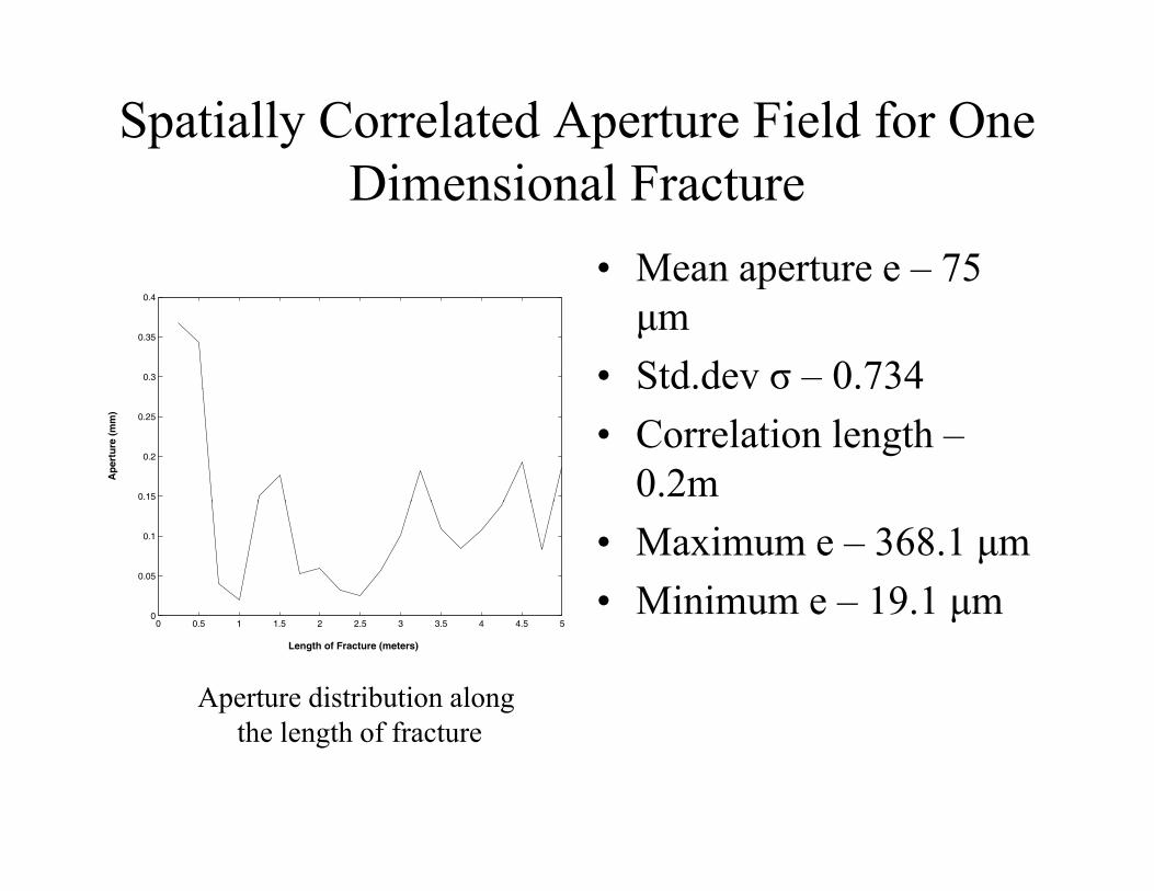
Spatially Correlated Aperture Field for One i i lDimensional Fracture
• Mean aperture e – 75Mean aperture e 75 μm
• Std.dev σ – 0.7340.3
0.35
0.4
• Correlation length –0.2m0.15
0.2
0.25
Ap
ertu
re (
mm
)
• Maximum e – 368.1 μm• Minimum e – 19.1 μm0
0.05
0.1
u e 9. μ0 0.5 1 1.5 2 2.5 3 3.5 4 4.5 5
0
Length of Fracture (meters)
Aperture distribution along th l th f f tthe length of fracture
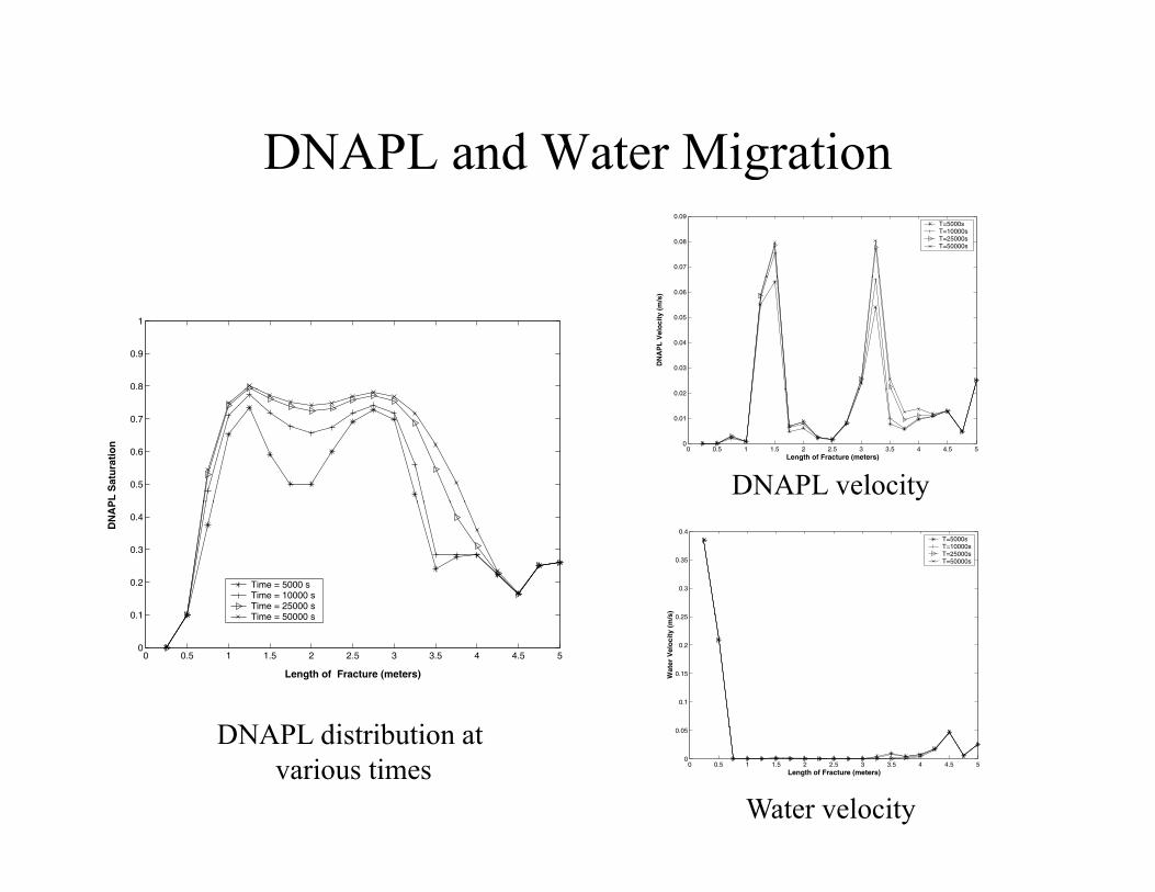
DNAPL and Water MigrationDNAPL and Water Migration
0.07
0.08
0.09T=5000sT=10000sT=25000s T=50000s
0.8
0.9
1
0.03
0.04
0.05
0.06
DN
AP
L V
elo
city
(m
/s)
0.5
0.6
0.7
PL
Sat
ura
tio
n
0 0.5 1 1.5 2 2.5 3 3.5 4 4.5 50
0.01
0.02
Length of Fracture (meters)
DNAPL velocity
0 1
0.2
0.3
0.4
DN
AP
Time = 5000 sTime = 10000 s Time = 25000 sTime 50000 s 0 25
0.3
0.35
0.4
s)
T=5000sT=10000sT=25000sT=50000s
0 0.5 1 1.5 2 2.5 3 3.5 4 4.5 50
0.1
Length of Fracture (meters)
Time = 50000 s
0.1
0.15
0.2
0.25
Wat
er V
elo
city
(m
/s
DNAPL di t ib ti t0 0.5 1 1.5 2 2.5 3 3.5 4 4.5 5
0
0.05
Length of Fracture (meters)
DNAPL distribution at various times
Water velocity
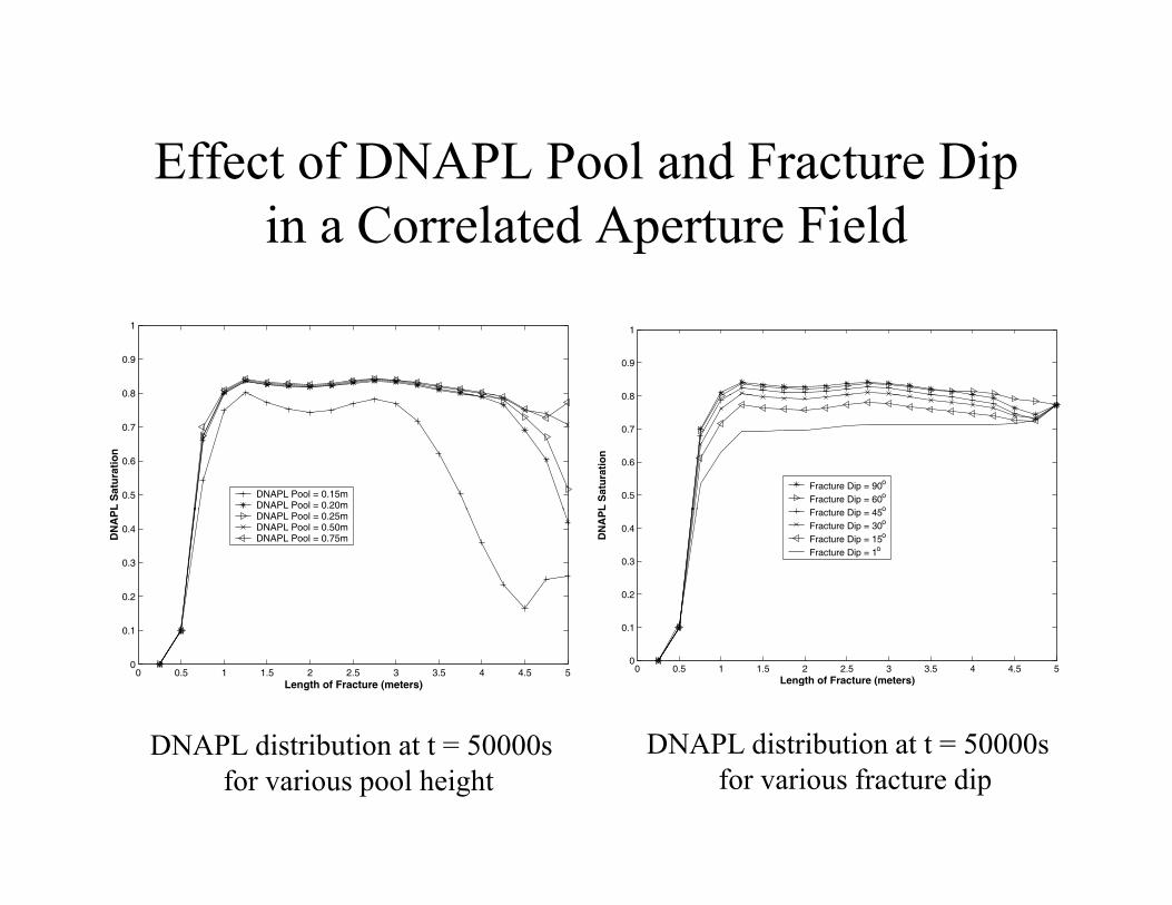
Effect of DNAPL Pool and Fracture DipEffect of DNAPL Pool and Fracture Dip in a Correlated Aperture Field
0.8
0.9
1
0 8
0.9
1
0.5
0.6
0.7
0.8
L S
atu
rati
on
DNAPL Pool = 0.15mDNAPL Pool = 0.20m
0.5
0.6
0.7
0.8
L S
atu
rati
on
Fracture Dip = 90o
Fracture Dip = 60o
F t Di 45o
0.2
0.3
0.4
DN
AP DNAPL Pool = 0.25m
DNAPL Pool = 0.50mDNAPL Pool = 0.75m
0.2
0.3
0.4
DN
AP
L Fracture Dip = 45o
Fracture Dip = 30o
Fracture Dip = 15o
Fracture Dip = 1o
0 0.5 1 1.5 2 2.5 3 3.5 4 4.5 50
0.1
Length of Fracture (meters)
0 0.5 1 1.5 2 2.5 3 3.5 4 4.5 50
0.1
Length of Fracture (meters)
DNAPL di t ib ti t t 50000 DNAPL di t ib ti t t 50000DNAPL distribution at t = 50000s for various pool height
DNAPL distribution at t = 50000s for various fracture dip

Effect of Correlation Length on DNAPL d i iand Water Migration
0.4
0.45
0.5
correlation length = 100 mm correlation length = 200 mm correlation length = 300 mm
Nodal Discretization = 250 mm
0.08
0.09
0.1
correlation length=200mm
0.15
0.2
0.25
0.3
0.35
Fra
ctu
re A
per
ture
(m
m)
correlation length = 300 mm correlation length = 400 mm
0.03
0.04
0.05
0.06
0.07
DN
AP
L V
elo
city
(m
/s)
correlation length=300mm
correlationlength=400mm
0 0.5 1 1.5 2 2.5 3 3.5 4 4.5 50
0.05
0.1
Length of Fracture (meters)0 0.5 1 1.5 2 2.5 3 3.5 4 4.5 5
0
0.01
0.02
Length of Fracture (meters)
correlation length=100mm
Aperture distribution DNAPL velocity at t = 50000s
0 6
0.7
0.8
0.9
1
on
correlation length = 200mm
correlation length = 300mm 0.5
0.6
0.7
m/s
)
correlation length = 400mm
correlation length = 300mm
0.2
0.3
0.4
0.5
0.6
DN
AP
L S
atu
rati
o
correlation length = 400mm
0.1
0.2
0.3
0.4
Wat
er V
elo
city
(m
correlation length = 200mm
correlation length = 100mm
0 0.5 1 1.5 2 2.5 3 3.5 4 4.5 50
0.1
Length of Fracture (meters)
correlation length = 100mm
0 0.5 1 1.5 2 2.5 3 3.5 4 4.5 50
Length of Fracture (meters)
DNAPL distribution at t = 50000s Water velocity at t = 50000s

Range of Apertures for Various Fracture A fi ld dAperture fields generated
Correlation Maximum Minimum Aperture at Aperture justlengths
mm
aperture
μm
aperture
μm
the top of fractureμm
below the top cellμmmm μm μm μm μm
100 368.1 24.9 27.722 24.926
200 368.1 19.1 186.77 82.627
300 469.1 19.8 144.57 182.41
400 466.5 19.0 40.033 25.1
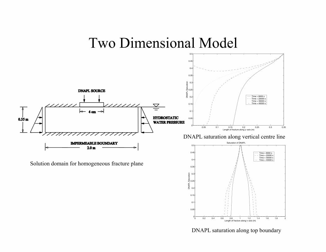
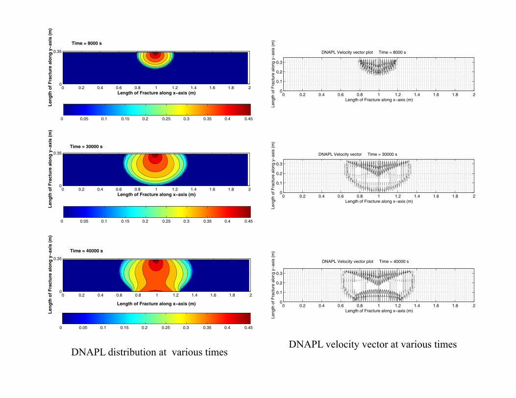
Two Dimensional ModelTwo Dimensional Model
0.35
0.4
0.45
0.5
0.15
0.2
0.25
0.3
DN
AP
L S
atur
atio
n
Time = 8000 sTime = 20000 sTime = 30000 sTime = 40000 s
0.05 0.1 0.15 0.2 0.25 0.3 0.350
0.05
0.1
Length of fracture along y−axis (m)
DNAPL saturation along vertical centre line
Solution domain for homogeneous fracture plane0 3
0.35
0.4
0.45
0.5
n
Time = 8000 sTime = 20000 sTime = 30000 sTime = 40000 s
Saturation of DNAPL
0.1
0.15
0.2
0.25
0.3
DN
AP
L S
atur
atio
0 0.2 0.4 0.6 0.8 1 1.2 1.4 1.6 1.8 20
0.05
Length of fracture along x−axis (m)
DNAPL saturation along top boundary
0.35tu
re a
lon
g y−a
xis
(m)
Time = 8000 s
0.2
0.3
e al
ong
y−ax
is (
m)
DNAPL Velocity vector plot Time = 8000 s
0 0.05 0.1 0.15 0.2 0.25 0.3 0.35 0.4 0.45
0 0.2 0.4 0.6 0.8 1 1.2 1.4 1.6 1.8 20
Length of Fracture along x−axis (m)
Len
gth
of
Fra
ct
0 0.2 0.4 0.6 0.8 1 1.2 1.4 1.6 1.8 20
0.1
Length of Fracture along x−axis (m)
Leng
th o
f Fra
ctur
e
0.35
ure
alo
ng
y−a
xis
(m)
Time = 30000 s
0 2
0.3
alo
ng y−
axis
(m
)
DNAPL Velocity vector Time = 30000 s
0 0.05 0.1 0.15 0.2 0.25 0.3 0.35 0.4 0.45
0 0.2 0.4 0.6 0.8 1 1.2 1.4 1.6 1.8 20
Length of Fracture along x−axis (m)
Len
gth
of
Fra
ctu
0 0.2 0.4 0.6 0.8 1 1.2 1.4 1.6 1.8 20
0.1
0.2
Length of Fracture along x−axis (m)
Leng
th o
f Fra
ctur
e
0.35
e al
on
g y−a
xis
(m)
Time = 40000 s
0.3g y−
axis
(m
)
DNAPL Velocity vector plot Time = 40000 s
0 0.2 0.4 0.6 0.8 1 1.2 1.4 1.6 1.8 20
Length of Fracture along x−axis (m)
Len
gth
of
Fra
ctu
re
0 0.2 0.4 0.6 0.8 1 1.2 1.4 1.6 1.8 20
0.1
0.2
0.3
Length of Fracture along x−axis (m)
Leng
th o
f Fra
ctur
e al
on
0 0.05 0.1 0.15 0.2 0.25 0.3 0.35 0.4 0.45
DNAPL distribution at various timesDNAPL velocity vector at various times

0.35
ctu
re a
lon
g y−a
xis
(m)
Fracture Aperture = 25 μm
0 0.05 0.1 0.15 0.2 0.25 0.3 0.35 0.4 0.45
0 0.2 0.4 0.6 0.8 1 1.2 1.4 1.6 1.8 20
Length of Fracture along x−axis (m)
Len
gth
of
Fra
c0.35
alo
ng
y−a
xis
(m)
Fracture Aperture = 35 μm
Base case
0 0.2 0.4 0.6 0.8 1 1.2 1.4 1.6 1.8 20
Length of Fracture along x−axis (m)
Len
gth
of
Fra
ctu
re
0 0.05 0.1 0.15 0.2 0.25 0.3 0.35 0.4 0.45
0.35
ng
y−a
xis
(m)
Horizontal Fracture
Effect of aperture
0 0.2 0.4 0.6 0.8 1 1.2 1.4 1.6 1.8 20
Length of Fracture along x−axis (m)
eng
th o
f F
ract
ure
alo
n
0 0.05 0.1 0.15 0.2 0.25 0.3 0.35 0.4 0.45
Le
Effect of dip

DNAPL Courant Number

Effect of Heterogeneity
0.5 0.5T = 8000sT 30000s
DNAPL Saturation
Solution domain for heterogeneous fracture plane
0.3
0.35
0.4
0.45
tura
tion
0.3
0.35
0.4
0.45
urat
ion
T = 30000sT = 40000s
0.1
0.15
0.2
0.25
DN
AP
L S
at
Time = 8000 sTime = 30000 sTime = 40000 s
0.1
0.15
0.2
0.25
DN
AP
L S
atu
0 0.05 0.1 0.15 0.2 0.25 0.3 0.350
0.05
Length of Fracture along y−axis (m)0 0.2 0.4 0.6 0.8 1 1.2 1.4 1.6 1.8 2
0
0.05
Length of Fracture along x−axis (m)
DNAPL saturation along vertical centre line DNAPL saturation along top boundary

Effect of Heterogeneity on DNAPL Mi tiMigration
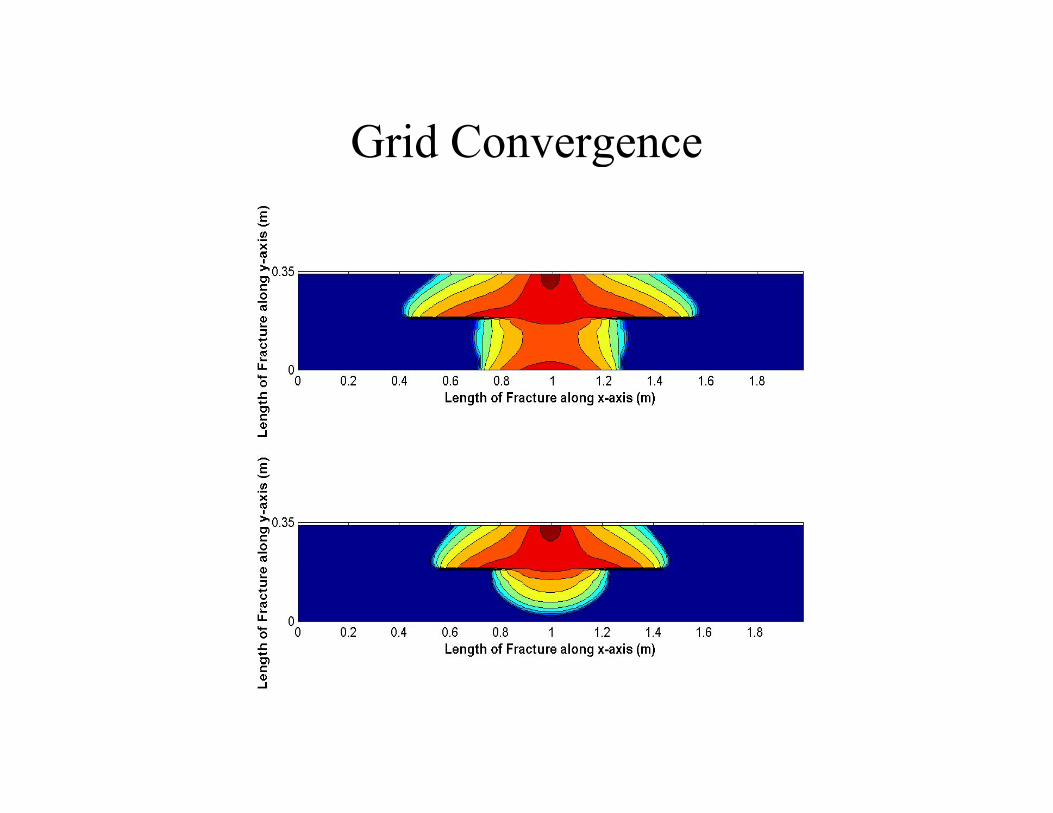
Grid ConvergenceGrid Convergence
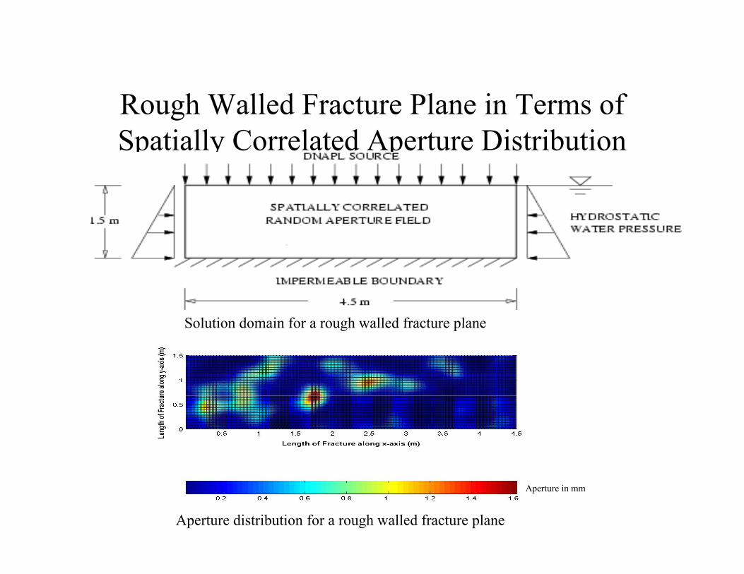
Rough Walled Fracture Plane in Terms ofRough Walled Fracture Plane in Terms of Spatially Correlated Aperture Distribution
Solution domain for a rough walled fracture planeSolution domain for a rough walled fracture plane
Aperture in mm
Aperture distribution for a rough walled fracture plane
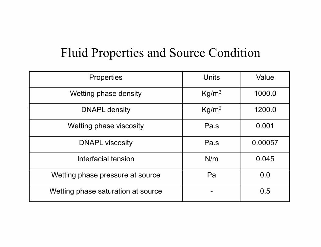
Fluid Properties and Source Condition
Properties Units ValueProperties Units Value
Wetting phase density Kg/m3 1000.0
DNAPL d it K / 3 1200 0DNAPL density Kg/m3 1200.0
Wetting phase viscosity Pa.s 0.001
DNAPL viscosity Pa.s 0.00057
Interfacial tension N/m 0.045
Wetting phase pressure at source Pa 0.0
Wetting phase saturation at source - 0.5

Range of Apertures in the Field GeneratedRange of Apertures in the Field Generated
0.6
0.7Along the topAlong the bottom
3.5
4
4.5x 10
−8
Along the topAlong the bottom
0.3
0.4
0.5
riatio
n of
Ape
rture
(mm
)
2
2.5
3
mea
bilit
y of
Fra
ctur
e (m
2 )
0 0.5 1 1.5 2 2.5 3 3.5 4 4.50
0.1
0.2
Length of Fracture along x axis (m)
Var
0 0.5 1 1.5 2 2.5 3 3.5 4 4.50
0.5
1
1.5
Length of Fracture along x axis (m)
Perm
Length of Fracture along x−axis (m) Length of Fracture along x−axis (m)
Aperture distribution along the top and bottom boundary Fracture permeability along the top and bottom boundary
Range of apertures within a fracture
Range Unit Domain Top boundary Bottom boundary
Maximum μm 1615 1 695 73 340 53
g p
Maximum μm 1615.1 695.73 340.53
minimum μm 30.231 30.231 44.234
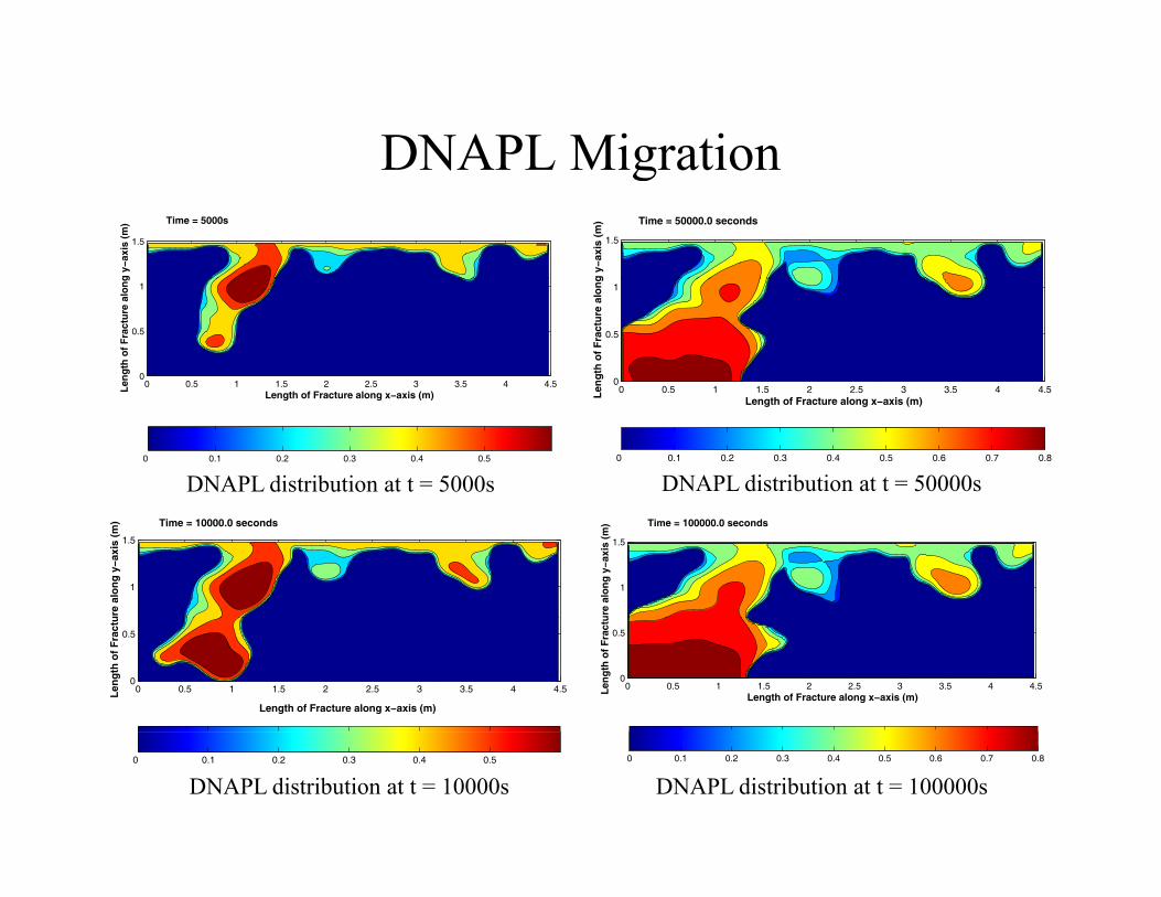
DNAPL MigrationDNAPL Migration1.5
g y−a
xis
(m) Time = 5000s
1.5
g y−a
xis
(m) Time = 50000.0 seconds
0 0.5 1 1.5 2 2.5 3 3.5 4 4.50
0.5
1
L th f F t l i ( )
Len
gth
of
Fra
ctu
re a
lon
g
0 0.5 1 1.5 2 2.5 3 3.5 4 4.50
0.5
1
eng
th o
f F
ract
ure
alo
ng
0 0.1 0.2 0.3 0.4 0.5
Length of Fracture along x−axis (m)
0 0.1 0.2 0.3 0.4 0.5 0.6 0.7 0.8
0 0.5 1 1.5 2 2.5 3 3.5 4 4.5Length of Fracture along x−axis (m)
L
DNAPL distribution at t = 5000s DNAPL distribution at t = 50000s
1
1.5
ure
alo
ng
y−a
xis
(m) Time = 10000.0 seconds
1
1.5
ure
alo
ng
y−a
xis
(m) Time = 100000.0 seconds
0 0.5 1 1.5 2 2.5 3 3.5 4 4.50
0.5
Length of Fracture along x−axis (m)
Len
gth
of
Fra
ctu
0 0.5 1 1.5 2 2.5 3 3.5 4 4.50
0.5
Length of Fracture along x−axis (m)
Len
gth
of
Fra
ctu
0 0.1 0.2 0.3 0.4 0.5 0 0.1 0.2 0.3 0.4 0.5 0.6 0.7 0.8
DNAPL distribution at t = 10000s DNAPL distribution at t = 100000s

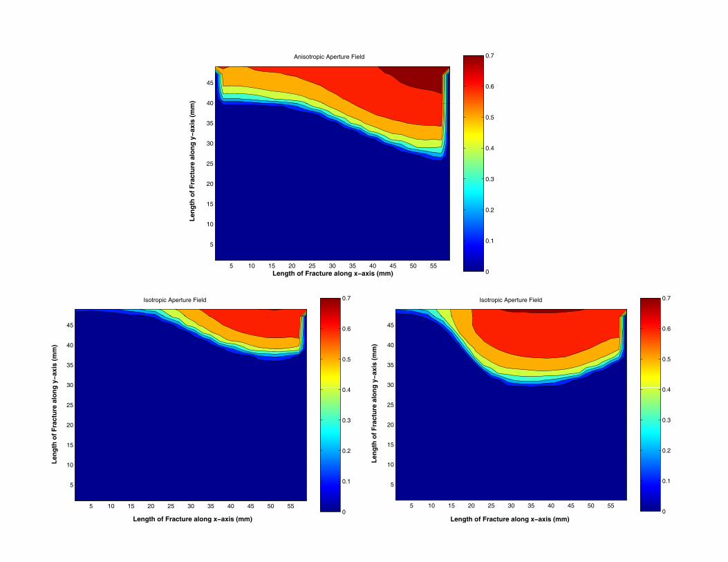
Isotropic and Anisotropic Aperture FieldIsotropic and Anisotropic Aperture Field
0.11
45
Aperture (mm)
0.06
0.07
0.08
0.09
0.1
20
25
30
35
40
45
Fra
ctu
re a
lon
g y−a
xis
(mm
)
0.02
0.03
0.04
0.05
5 10 15 20 25 30 35 40 45 50 55
5
10
15
Length of Fracture along x−axis (mm)
Len
gth
of
C l ti l th (30 30)
0.25
0.3
40
45
mm
)
Aperture (mm)
0.12
40
45
s (m
m)
Aperture (mm) Solution domain
Correlation length (30,30)mm
0.15
0.2
10
15
20
25
30
35
Len
gth
of
Fra
ctu
re a
lon
g y−a
xis
(m
0.06
0.08
0.1
10
15
20
25
30
35
Len
gth
of
Fra
ctu
re a
lon
g y−a
xis
0.1
5 10 15 20 25 30 35 40 45 50 55
5
10
Length of Fracture along x−axis (mm)
0.02
0.04
5 10 15 20 25 30 35 40 45 50 55
5
10
Length of Fracture along x−axis (mm)
Correlation length (30,20)mm Correlation length (20,20)mm
0.6
0.7
40
45
m)
Anisotropic Aperture Field
0.4
0.5
25
30
35
40
ctu
re a
lon
g y−a
xis
(mm
0.1
0.2
0.3
5
10
15
20L
eng
th o
f F
rac
0.7Isotropic Aperture Field
0 5 10 15 20 25 30 35 40 45 50 55
5
Length of Fracture along x−axis (mm)
0.7Isotropic Aperture Field
0.5
0.6
30
35
40
45
g y−a
xis
(mm
)
0 4
0.5
0.6
30
35
40
45
g y−a
xis
(mm
)
0.2
0.3
0.4
15
20
25
eng
th o
f F
ract
ure
alo
ng
0.2
0.3
0.4
15
20
25
eng
th o
f F
ract
ure
alo
ng
0
0.1
5 10 15 20 25 30 35 40 45 50 55
5
10
Length of Fracture along x−axis (mm)
Le
0
0.1
5 10 15 20 25 30 35 40 45 50 55
5
10
Length of Fracture along x−axis (mm)
Le

Buoyancy flow and Capillary Trapping
Local capillary Gravity fingering
Buoyancy flow -most dense fluid- downward, lateral and lidi tp y
trapping sliding movement
Gravity fingering - once the residual DNAPL pools up on the top of the wedge
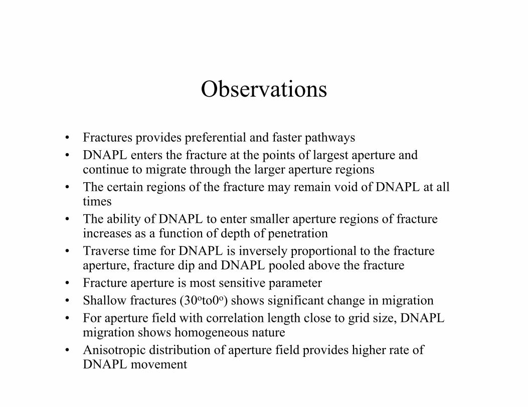
Observations
• Fractures provides preferential and faster pathways• DNAPL enters the fracture at the points of largest aperture and
continue to migrate through the larger aperture regions• The certain regions of the fracture may remain void of DNAPL at all
times • The ability of DNAPL to enter smaller aperture regions of fracture
i f i f d h f iincreases as a function of depth of penetration• Traverse time for DNAPL is inversely proportional to the fracture
aperture, fracture dip and DNAPL pooled above the fractureF t t i t iti t• Fracture aperture is most sensitive parameter
• Shallow fractures (30oto0o) shows significant change in migration • For aperture field with correlation length close to grid size, DNAPL
migration shows homogeneous naturemigration shows homogeneous nature• Anisotropic distribution of aperture field provides higher rate of
DNAPL movement

ImmiscibleImmiscible--miscible flow in coastal miscible flow in coastal iireservoirsreservoirs
Seawater intrusion is an ideal problem to study the buoyancy flow
Natural intrusion of heavier fluid with matched viscosity

Ghyben-Herzberg approximation for seawater intrusion
Groundwater flow patterns in an idealized,
homogeneous coastal aquifer. (Source: USGS)q ( )
•Analytical solution on the basis of Ghyben-herzberg Relationship(Bear,1972) and Single Potential Theory (strack,1976).•The assumption of a sharp interface between freshwater andsaltwater.
1082/10/2012
•Variable density flow in both time and space dimension (Frind,1982;Voss and Souza; Kolditz et al.,1998).

Immiscible-miscible flow of Seawater - freshwater• A freshwater confined aquifer of size 2m by 1m,
I bl b d diti th t• Impermeable boundary conditions on the topand bottom.
• The left open boundary, a constant freshwaterinflux (qf =6.6x10⁻⁵ m2/s, ρf=1000 kg/ m3, μf=10-3 m2/s)3 m2/s)
• The open right hand boundary, a hydrostaticpressure distribution (ρs=1025 kg/ m3, μs=10-3m2/s)
• 50 % saltwater saturation (S ) is assumed• 50 % saltwater saturation (SS) is assumed• 25 % of the vertical dimension of the aquifer is
assumed to be freshwater mouth.
The interface between the 2 fluids is sharp without
any smearingany smearing
Seawater saturation contours at 6000 seconds
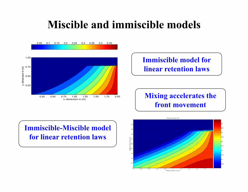
Miscible and immiscible models
1.00
0.05 0.1 0.15 0.2 0.25 0.3 0.35 0.4 0.45
Immiscible model for
−dim
ensi
on in
(m)
0.50
0.75
Immiscible model for linear retention laws
x−dimension in (m)
y−
0.25 0.50 0.75 1.00 1.25 1.50 1.75 2.00
0.25
Mixing accelerates the front movement
Immiscible-Miscible model for linear retention laws
110

Miscible and immiscible models
Immiscible model for li t ti llinear retention laws
Mixing accelerates the front movement
Immiscible-Miscible model for linear retention laws
111

With buoyancy
Effect of freshwater flux
buoyancy
Without buoyancy
Effect of buoyancyEffect of buoyancy
Buoyancy in a multiphase model acts as a dispersive
Freshwater flux reduced to half
mechanism

Effect of relative permeability on the seawater-freshwater transition zone
B k C Linear relationBrooks - Corey Linear relation
Quadratic relation
Cubic relationCubic relation shows nearest
resemblance to Brooks - Corey

Effect of relative permeability on the seawater-freshwater transition zone

3-Phase Immiscible Flow in Coastal Reservoir(Buoyancy Flow and Capillary Trapping)(Buoyancy Flow and Capillary Trapping)
Seawater intrusionSeawater intrusion and oil migration oil migration in ain a coastal aquifer
This study is done to demonstrate buoyancy This study is done to demonstrate buoyancy flow and capillary trapping in immiscible flowflow and capillary trapping in immiscible flow
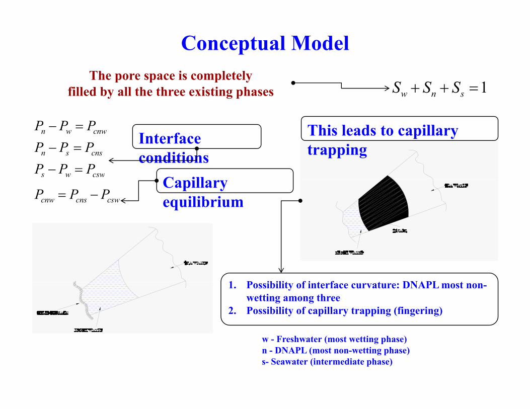
Conceptual ModelThe pore space is completely
1=++ snw SSS
PPP =−
The pore space is completely filled by all the three existing phases
Thi l d t ill
cswws
cnssn
cnwwn
PPPPPPPPP
=−=−=
Interface conditions
C ill
This leads to capillary trapping
cswcnscnw PPP −=Capillary equilibrium
1 P ibilit f i t f t DNAPL t1. Possibility of interface curvature: DNAPL most non-wetting among three
2. Possibility of capillary trapping (fingering)
w - Freshwater (most wetting phase)n - DNAPL (most non-wetting phase)s- Seawater (intermediate phase)

)( rnnsd
SSSPP −+=
Linear relation for capillary pressure (conditions for the interfaces)
)0.1( rwrndcnw SSPP
−−
)01()( rnrwnw
dcns SSSSSSPP
−−−−+
−=
( )
)0.1( rwrn SS
Non-linear relation (Brooks-Corey) for relative permeability of phases
( )( )
rwwew SS
SSS −=
01
(conditions for the interfaces)
( )3( )4ewrw Sk =
( )rnrw SS −−0.1
( )rnrw
ses SS
SS−−
=0.1
( ) )0.2(3esesrs SSk −=
( ) )0.1(3ewesenrn SSSk +−=
( )rnrw
rnnen SS
SSS−−
−=
0.1
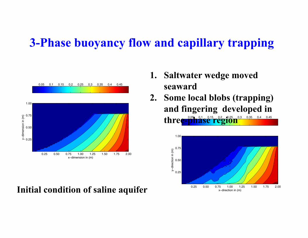
3-Phase buoyancy flow and capillary trapping3-Phase buoyancy flow and capillary trapping
1 Saltwater wedge moved
1.00
0.05 0.1 0.15 0.2 0.25 0.3 0.35 0.4 0.45
1. Saltwater wedge moved seaward
2. Some local blobs (trapping)
men
sion
in (
m)
0.50
0.75
1.00
0.05 0.1 0.15 0.2 0.25 0.3 0.35 0.4 0.45
and fingering developed in three-phase region
x−dimension in (m)
y−di
0.25 0.50 0.75 1.00 1.25 1.50 1.75 2.00
0.25
ectio
n in
(m
)
0.50
0.75
1.00
x−direction in (m)
y−di
re
0.25 0.50 0.75 1.00 1.25 1.50 1.75 2.00
0.25
Initial condition of saline aquiferq

Buoyancy flow and Capillary Trapping
Local capillary Gravity fingering
Buoyancy flow -most dense fluid- downward, lateral and lidi ttrapping sliding movement
Gravity fingering - once the residual DNAPL pools up on the top of the wedge
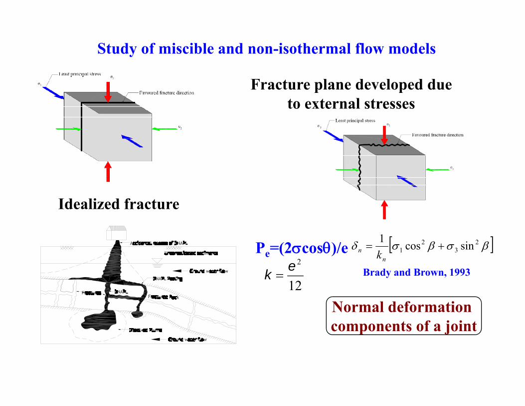
Study of miscible and non-isothermal flow models
Fracture plane developed due to external stresses
Idealized fracture plane
[ ]βσβσδ 23
21 sincos1
+=n
n kBrady and Brown, 1993
p
2ek =
Pe=(2σcosθ)/e
Normal deformation components of a joint
12
co po e ts o a jo t

Coupling Deformation with Fluid Pressures
[ ]wn
n Pk
−+= βσβσδ 23
21 sincos1Assumption
Modifiednormal
d f ti If P >P
n
deformation If Pw >Pn
If Pw <Pn
[ ]nn P−+= βσβσδ 23
21 sincos1 [ ]n
nn k
ββ 31
Coupling Deformation with I i ibl fl M d l
121
Immiscible flow ModelAperture of fracture, et nt ee δ±= 0
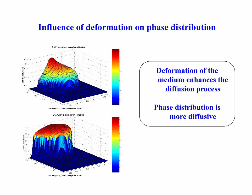
Influence of deformation on phase distribution
Deformation of the medium enhances the
diffusion process
Phase distribution is more diffusive

Influence of deformation on energy transfer
Deformation of the medium enhances
th diff ithe diffusion process

Influence of deformation on mass transfer
Deformation of the mediumDeformation of the medium enhances the diffusion
process
Mass transfer diffuses very fast
In the storage system this kind of diffusive processkind of diffusive process
secures better storage

Immiscible flow with miscible, non-isothermal and medium deformationmedium deformation
• This test problem shows that immiscible flow systemp yshould be coupled with miscible and non-isothermalflow which can represent the complete multiphasesystem
• Also the medium deformation through hydro-mechanical coupling should be considered if the
lti h fl t h t b id d imultiphase flow system has to be considered in anygeological environment, shallow or deep

Thank YouThank YouThank YouThank You