Multiobjective shortest path problems with lexicographicgoal-based preferences

Francisco Javier Pulidoa,∗, Lawrence Mandowa,∗∗, José Luis Pérez de la Cruza

aDpto. Lenguajes y Ciencias de la ComputaciónUniversidad de Málaga

Boulevar Louis Pasteur, 35. Campus de Teatinos, 29071 - Málaga (Spain)

Abstract

Multiobjective shortest path problems are computationally harder than single objective ones.In particular, execution time is an important limiting factor in exact multiobjective search al-gorithms. This paper explores the possibility of improving search performance in those caseswhere the interesting portion of the Pareto front can be initially bounded. We introduce a newexact label-setting algorithm that returns the subset of Pareto optimal paths that satisfy a set oflexicographic goals, or the subset that minimizes deviation from goals if these cannot be fullysatisfied. Formal proofs on the correctness of the algorithm are provided. We also show that thealgorithm always explores a subset of the labels explored by a full Pareto search. The algorithmis evaluated over a set of problems with three objectives, showing a performance improvementof up to several orders of magnitude as goals become more restrictive.

Keywords:Combinatorial optimization, Multiobjective Shortest Path Problem, Best-first search, Heuristicsearch, Goal programming, Artificial Intelligence

1. Introduction

Goal programming is one of the most successful models of Multicriteria Decision Theory(Chankong and Haimes, 1983). Virtually hundreds of applications can be found in the litera-ture (Romero, 1991; Tamiz et al., 1995). This paper explores the application of the goal-baseddecision paradigm to multicriteria shortest path problems.

Multicriteria shortest path problems arise naturally in many fields, such as robot surveillance(Delle Fave et al., 2009), robot path planning (Fujimura, 1996), satellite scheduling (Gabrel andVanderpooten, 2002), and route planning in different contexts (Machuca and Mandow, 2012;Jozefowiez et al., 2008; Clímaco et al., 2003; Delling and Wagner, 2009). A number of shortestpath algorithms have been proposed to tackle different multicriteria decision models. The workof Hansen (1979) presented a bi-objective extension of Dijkstra’s label setting algorithm. Martins

∗Main Corresponding author, Tel. +34 (9)52 132863∗∗Corresponding author

Email addresses: francis@lcc.uma.es (Francisco Javier Pulido), lawrence@lcc.uma.es (LawrenceMandow), perez@lcc.uma.es (José Luis Pérez de la Cruz)Preprint submitted to European Journal of Operational Research, www.elsevier.com/locate/ejorMay 2, 2014

(1984) proposed a general multiobjective label setting algorithm. A recent evaluation of severalmultiobjective shortest path algorithms can be found in (Raith and Ehrgott, 2009).

The multiobjective shortest path problem is computationally harder than the single objectiveone. The number of label expansions can grow exponentially with solution depth, even forthe two objective case (Hansen, 1979). With the assumption of bounded integer costs and afixed number of objectives the problem becomes tractable for polynomially sized graphs, butstill harder than single objective search (e.g. see (Mandow and Pérez de la Cruz, 2009; Müller-Hannemann and Weihe, 2006)).

Search efficiency can be improved in single destination (one to one) problems using lowerbound distance estimates in a similar way as algorithm A* improves over Dijkstra’s (Pearl,1984). Several multiobjective extensions of A* have been proposed. These can be groupedin two classes: those that perform node expansion as its basic operation (like MOA∗ (Stewartand White, 1991)), and those that perform label expansion (like Tung and Chew’s algorithm(Tung and Chew, 1992) and NAMOA∗ (Mandow and Pérez de la Cruz, 2010)). The interest inthese algorithms with lower bounds is justified by the fact that: precise lower bound estimatescan be efficiently precalculated for a large class of problems (Tung and Chew, 1992); and the useof such estimates still guarantees an exact solution, i.e. the algorithms find the set of all Paretooptimal solutions to the problem.

Several algorithms extended the node expansion policy of MOA* to different contexts, likealgorithms MOA∗∗ for search with nonconsistent lower bounds (Dasgupta et al., 1999), BCA∗

for compromise solutions (Galand and Perny, 2006), or METAL-A∗ for goal based preferences(Mandow and Pérez de la Cruz, 2001). The latter are the subject of this work. However, recentempirical and formal analyses (Machuca et al., 2012; Pérez et al., 2013) have shown that lowerbounded search with node expansion can perform much worse than blind search algorithms and,more precisely, that performance can seriously degrade with better lower bound estimates. Inpractice, this result ruins the primary purpose of using lower bounds in these algorithms in thefirst place.

On the other hand, label expansion algorithms with lower bounds have successfully improvedperformance over blind search algorithms. The efficiency of NAMOA∗ has been formally shownto improve with better informed lower bound estimates and, in fact, it has been shown to opti-mally exploit such estimates among the class of admissible algorithms (Mandow and Pérez dela Cruz, 2010). Empirical results confirm that NAMOA∗ performs consistently better than blindsearch, and that better informed lower bounds result in faster search with less space requirements(Machuca et al., 2012). Experiments on problems like bicriteria route planning reveal that time,rather than space, is the practical limiting factor in the calculation of the full Pareto set of so-lutions (Machuca and Mandow, 2012; Machuca et al., 2009). Recent attempts to improve thisalgorithm include parallel search (Sanders and Mandow, 2013) and the use of specific efficientdata structures (Mali et al., 2012).

Many problems do not require in practice the calculation of the full Pareto optimal set ofsolutions. In this work we investigate the possibility of further improvements over the efficiencyof NAMOA∗ through the introduction of lexicographic goal based preferences. A set of goalscan be proposed to bound the area of interesting solutions. More precisely, given a set of goals,we tackle the problem of finding the subset of Pareto optimal paths that satisfy the goals or, ifthese cannot be satisfied, finding the subset of Pareto optimal paths that minimize deviation fromthe goals. We propose a new multicriteria label-setting algorithm with lower bounds and labelexpansion that finds such goal-optimal solutions. The new algorithm explores a subset of thelabels explored by NAMOA∗, achieving important performance improvements.

2

Section 2 reviews relevant concepts from multicriteria decision theory and introduces theconcept of pruning preference. Section 3 describes the algorithm. Important properties concern-ing admissibility and efficiency are presented in section 4. An empirical evaluation is describedand discussed in section 5. Finally some conclusions and future work are outlined.

2. Preliminaries

2.1. Lexicographic goal preferences

First of all, we review the concepts of attribute, objective, and goal, as defined in Romero(1991). Let X be the set of solutions to a decision problem. An attribute is a measurableproperty g(x) : X → R. An objective represents the desired improvement of an attribute,i.e. maximization or minimization. A goal combines an attribute with a specific target value,or aspiration level t ∈ R, stated by the decision maker to define his/her preference. Goals formultiobjective shortest path problems are always of the form g(x) ≤ t. Goals are not constraints,i.e. feasible solutions may not satisfy all goals.

Let us consider a set of q attributes gi : X → R, 1 ≤ i ≤ q grouped in l priority levels sortedin order of decreasing preemptive importance. Each priority level k comprises a set Ik of one ormore attributes. Goals are defined by setting targets ti for each attribute, gi(x) ≤ ti.

A solution to a goal problem is satisfactory when all the goals can be satisfied. We seeknondominated satisfactory solutions. If there are no satisfactory solutions to a problem, we seeknondominated solutions that minimize deviation from the targets. In lexicographic goal prob-lems, the deviation of a set of goals is measured separately for each priority level. Minimizingthe deviation of goals at level k is infinitely more important than minimizing deviation at levelk + 1.

Several methods have been proposed to measure the deviation from a set of goals. In thiswork, the minimization of the weighted sum of deviations is employed. Let ~g = (g1, g2, ..., gq)be a vector with all attributes (costs) of a given solution x ∈ X . We can calculate a deviationvector for ~g with one component for each priority level, ~d(~g) = (d1(~g), d2(~g), ..., dl(~g)). Foreach level k, its deviation dk can be defined as:

dk(~g) =∑i∈Ik

wi ×max(0, gi − ti) (1)

where wi is the relative weight of goal i in level k.We define the optimum achievement vector ~d∗ = (d∗1, d

∗2, ..., d

∗l ) as the minimum lexico-

graphic deviation vector among all solutions. Thus, the set of goal-optimal solutions consistsof all nondominated feasible solutions with a deviation equal to ~d∗. If there is a satisfactorysolution, then the optimum achievement vector is equal to ~0.

2.2. Formal definitions

We will now reproduce some standard definitions and introduce some new preference rela-tions between cost vectors ~y, ~y′ ∈ Rq .

• Dominance (≺) or Pareto-optimal preference is defined as follows,

~y ≺ ~y′ ⇔ ∀i yi ≤ y′i ∧ ~y 6= ~y′ (2)

3

Dominance is a strict partial order. Given a set of vectors X , we shall defineN (X) the setof nondominated vectors in set X in the following way,

N (X) = {~x ∈ X | @~y ∈ X ~y ≺ ~x} (3)

We shall find it useful to denote by � the relation ”dominates or equals”.

• Let us denote αi = min~x∈N (X){xi}, and βi = max~x∈N (X){xi}. The set N (X) isbounded by the ideal point ~α = (α1 . . . αq), and the nadir point ~β = (β1 . . . βq). Theideal point can be calculated optimizing each objective separately. However, for q > 2 itis difficult to calculate the nadir point without computing the whole set of nondominatedsolutions.

• Lexicographic order ≺L is defined as follows,

~y ≺L ~y′ ⇔ ∃j yj < y′j ∧ ∀i < j yi = y′i. (4)

The lexicographic order is a strict total order. The lexicographic optimum of a set ofvectors is trivially a nondominated vector.

• We define lexicographic goal preferences (≺G) as a partial order relation,

~y ≺G ~y′ ⇔ ~d(~y) ≺L ~d(~y′) ∨ (~d(~y) = ~d(~y′) ∧ ~y ≺ ~y′) (5)

It is easy to see that ≺G is a strict partial order (it is irreflexive and transitive). Givena set of vectors X , we shall define OG(X) the set of optimal vectors in X according tolexicographic goal preferences (i.e. goal-optimal vectors) as,

OG(X) = {~x ∈ X | @~y ∈ X ~y ≺G ~x} (6)

Notice that an optimal solution according to ≺G is also a nondominated solution, i.e.OG(X) ⊆ N (X).

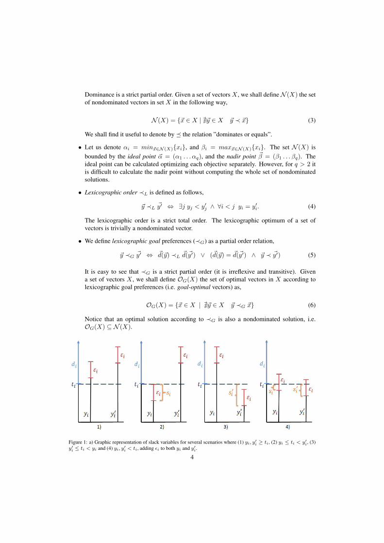
Figure 1: a) Graphic representation of slack variables for several scenarios where (1) yi, y′i ≥ ti, (2) yi ≤ ti < y′i, (3)y′i ≤ ti < yi and (4) yi, y′i < ti, adding εi to both yi and y′i.

4

• Let us consider a goal yk ≤ tk, the slack variable sk for this goal is defined as

sk = max(0, tk − yk) (7)

Let us assume two vectors ~y, ~y′ ∈ Rq and a level j such that dj(~y) < dj(~y′). Let us denote∆j(~y,~ε) = dj(~y + ~ε) − dj(~y). Obviously, if ~ε � ~0, ∆j(~y,~ε) ≥ 0. We define the cross-slack δj(~y, ~y′) = max~ε∈R+q (∆j(~y,~ε) −∆j(~y′,~ε)), i.e. the greatest relative increment ofthe deviations of ~y and ~y′ at level j when adding any ~ε ∈ R+q . Notice that δj(~y, ~y′) ≥ 0

and generally δj(~y, ~y′) 6= δj(~y′, ~y).

Figure 1 shows that for each i ∈ Ij four different cases can arise: (1) y′i, yi ≥ ti; (2)y′i ≥ ti and yi < ti; (3) y′i < ti and yi ≥ ti; (4) y′i, yi < ti. It is straightforward that thegreatest relative increment in cases 1 and 2 is 0, since the slack variable s′i equals 0, whilein cases 3 and 4, the greatest relative increment is wi × (s′i − si) . Therefore, an operativeway of calculating the cross-slack δj(~y, ~y′) of ~y, ~y′ at level j is

δj(~y, ~y′) =∑k∈Ij

wk ×max(0, s′k − sk) (8)

• We define the pruning preference ≺P by imposing on the lexicographical goal preferenceadditional conditions concerning cross-slacks:

~y ≺P ~y′ ⇔ ∃j (dj(~y) < dj(~y′) ∧ δj(~y, ~y′) < dj(~y′)− dj(~y)

∧ ∀i < j (di(~y) = di(~y′) ∧ δi(~y, ~y′) = 0)) (9)

i.e., ~y ≺P ~y′ when (i) ~y ≺G ~y′; (ii) the cross-slacks of ~y and ~y′ are zero for the first levels(where deviations are the same); and (iii) for the first level where deviations differ, thecross-slack of ~y and ~y′ is strictly smaller than the difference between deviations.

It can be easily checked that ≺P is irreflexive and transitive. Therefore ≺P is a partialorder relation. We read ~y ≺P ~y′ as «~y allows to prune ~y′».

2.3. Multicriteria shortest path problems

In the following, we shall be concerned with the evaluation of goals in multiobjective graphs,where the following definitions apply. Let G = (N,A,~c) be a locally finite labeled directedgraph, of |N | nodes, and |A| arcs (n, n′) labeled with positive cost vectors ~c(n, n′) ∈ Rq . Let apath in G be any sequence of nodes P = (n1, n2, ....nk) such that for all i < k, (ni, ni+1) ∈ A,and the cost vector of each path ~g(P ) = (g1(P ), g2(P ), ..., gq(P )) be the sum of the costsvectors of its component arcs.

A problem over a multiobjective graph is defined by a start node s ∈ N , and a destination1

node t. Each path in the graph, P = (s, ..., ni, ni+1, ..., t), represents a feasible solution to theproblem. A lower bound function ~h : N → Rq returns an estimate ~h(n) of the minimum costof all paths from n to t. A lower bound function ~h(n) is monotone if for all arcs (n, n′) in the

1Graph search literature often refers to this node as goal node. However, in this article we refer to it as destinationnode to avoid overloading the meaning of the word ”goal”.

5

graph, the following condition holds, ~h(n) � ~c(n, n′) + ~h(n′). ~h is admissible if ~h(n) neveroverestimates the cost of any path from n to t.

In the following we consider that the preference between solution paths is defined by a setof lexicographic goals. The solution to the problem is the set of all goal-optimal solutions (seeequation 5). We define the set of nondominated solutions as C∗ and the set of goal-optimalsolutions as C∗G, respectively. By definition, C∗G ⊆ C∗.

3. Algorithm LEXGO∗

This section introduces LEXGO∗, a multiobjective label-setting search algorithm for lexico-graphic goal preferences with lower bound estimates. The pseudocode of LEXGO∗ is shownin Table 1. The inputs are a multiobjective graph G, a start node s, a destination node t, a setof weighted goals grouped in preemptive priority levels, and a monotone lower bound function.LEXGO∗ outputs the set of all goal-optimal solution paths between s and t. The following datastructures are managed by the algorithm:

• SG: A search graph that records partial solution paths emanating from s and their costs.Each node n in SG stores the following information:

– Gop(n): Set of cost vectors (labels) ~gn of paths reaching node n which have not beenexplored yet.

– Gcl(n): Set of labels reaching node n which have already been explored.

• OPEN: A priority queue of unexplored labels. For each node n in SG and each cost vec-tor ~gn ∈ Gop(n), there is a label (n, ~gn) in OPEN. In fact, labels are extended to includealso evaluation vectors and their deviation from goals. Each extended label (n, ~dn, ~fn, ~gn)

denotes that node n is reached by a path with cost ~gn, deviation vector ~dn, and evalua-tion vector ~fn. We define ~fn = ~gn + ~h(n). For the sake of simplicity, we will denote~d(~fn) as ~dn. Initially, (s, ~ds, ~fs, ~gs) is the only label in OPEN. Labels in OPEN are sortedlexicographically according to deviation vectors. In case of ties they are ordered lexico-graphically according to evaluation vectors ~f . This ensures that the first element in thequeue has a goal-optimal evaluation.

• COSTS: The set of cost vectors of solution paths found to the destination node.

• Best achievement vector ~dB among all solutions already found.

The structure of LEXGO∗ is similar to previous label-setting multiobjective algorithms withlabel expansion, but incorporating elements of lexicographic goal preferences to guarantee thatonly a subset of the labels explored by a full multiobjective search will need to be explored.

The algorithm has five main steps. The first one is devoted to data structure initialization.The second one is devoted to label selection from OPEN, and lazy filtering. At each iteration thealgorithm selects the first label (n, ~dn, ~fn, ~gn) from OPEN, which has a goal-optimal evaluationvector. The label is removed from OPEN, and moved from Gop(n) to Gcl(n). The third steprecovers and returns the solution subgraph whenever some termination condition is satisfied. Thefourth step records the solution whenever a destination node is selected. COSTS and ~dB areupdated accordingly. Finally, the selected label is expanded in step 5, i.e. all the extensions ofthe selected label are considered for inclusion in the search graph and the OPEN set.

6

1. CREATE:—An empty search graph SG, and set s as its root.—Two sets Gcl(s) = ∅ and Gop(s) = {~0}.—A list of alternatives, OPEN = {(s, ~d(~h(s)),~h(s),~0}.—An empty set, COSTS.—~dB = ~∞, optimum achievement vector for solutions found.

2. PATH SELECTION. If OPEN is not empty, then,—Select a label (n, ~dn, ~fn, ~gn) from OPEN such that@(n′, ~dn′ , ~fn′ , ~gn′) ∈ OPEN | ~fn′ ≺G ~fn.—Delete the selected label from OPEN, and move ~gn from Gop(n) to Gcl(n).—If ∃~c∗ ∈ COSTS | ~c∗ ≺ ~fn, then repeat step 2 (lazy filtering)

3. CHECK TERMINATION. If OPEN is empty, or ~dB ≺L ~dn, then backtrack in SG from tand return the set of solution paths with costs in COSTS.

4. SOLUTION RECORDING. If n is a destination node, then—Include ~gn in COSTS.—~dB ←− ~dn—Go back to step 2.

5. PATH EXPANSION: If n is not a destination node, then for all successor nodes m of ndo:

(a) Calculate the cost of the new path found to m, its evaluation vector and deviation,~gm = ~gn + ~c(n,m), ~fm = ~gm + ~h(m), ~dm = ~d(~fm).

(b) If no Pareto or deviation filtering (equations 13 and 14), then:• If m /∈ SG:

– Add (m, ~dm, ~fm, ~gm) to OPEN– Set Gop(m) = {(~gm)}.– Label with ~gm a pointer from m to n.

• else if ~gm equals some cost vector in Gop(m) ∪Gcl(m) then– Label with ~gm a pointer from m to n.

• else if no Pareto or deviation pruning (equations 11 and 12), then:i. Eliminate vectors ~g′m ∈ Gop(m) | ~gm ≺ ~g′m ∨ ~fm ≺P ~g′m + ~h(m),

and their corresponding labels (m, ~d′m, ~f ′m, ~g′m) from OPEN.

ii. Add (m, ~dm, ~fm, ~gm) to OPEN, ~gm to Gop(m) and label with ~gm a pointerfrom m to n.

(c) Go back to step 2.

Table 1: Algorithm LEXGO∗

7

The algorithm iterates over steps 2,3,4 and 5 until OPEN is empty, or ~dB ≺L ~dn, i.e. allpotential goal-optimal solutions have been examined. In such case, the algorithm terminatesreturning a solution subgraph, made up of all goal-optimal solution paths. COSTS stores theset of distinct goal-optimal costs.

During path expansion two different conditions may prevent an extension from consideration:filtering and pruning. These are described in detail below.

3.1. Pruning conditionsRegrettably, the optimality principle does not hold for lexicographic goal preferences, i.e. a

goal-optimal path is not made of goal-optimal subpaths. The following example illustrates thisfact.

Example 1. Let us consider a search problem in a multiobjective graph with start node s, adestination node t, and the following preferences over three different attributes,

Level 1: g1 ≤ 20, w1 = 1.0Level 2: g2 ≤ 20, w2 = 0.5

g3 ≤ 20, w3 = 0.5(10)

Let us further assume the graph has two different paths P1 and P2 reaching some node n,where ∀n ~h(n) = (0, 0, 0), and the following costs and associated deviations,

~g(P1) = ~f(P1) = (15, 16, 22) ⇒ ~d(P1) = (0, 1)

~g(P2) = ~f(P2) = (20, 12, 16) ⇒ ~d(P2) = (0, 0)

We observe that ~f(P2) ≺G ~f(P1), since ~d(P2) ≺L ~d(P1). However, we cannot discard P1

in favor of P2. Let us now consider there is only one additional path P3 = (n, . . . , t) from n tothe destination node with cost ~g(P3) = (4, 4, 4). It is easy to show now that the concatenationP1P3 is the only goal-optimal solution,

~g(P1P3) = (19, 20, 26) ⇒ ~d(P1P3) = (0, 3)

~g(P2P3) = (24, 16, 20) ⇒ ~d(P2P3) = (4, 0)

Therefore, pruning and filtering using goal preferences would not yield an admissible labelsetting algorithm in this case. Nevertheless, LEXGO∗ includes two pruning conditions that im-prove search efficiency and, at the same time, guarantee that no goal-optimal solution will bepruned, (see Theorem 2 in Section 4 below):

• Pareto pruning. As in other Pareto search algorithms like NAMOA∗, we prune any domi-nated path to any node. A new label (m, ~dm, ~fm, ~gm) to node m is pruned whenever

∃~g ∈ Gop(m) ∪Gcl(m) | ~g ≺ ~gm (11)

• Deviation-based pruning. We propose an additional specific pruning condition based inthe pruning preference defined by equation 9. We prune a new label (m, ~dm, ~fm, ~gm) tonode m whenever,

∃~g ∈ Gop(m) ∪Gcl(m) | ~g + ~h(m) ≺P ~fm (12)8

Example 2. Let us assume the same preference as in example 1 and two paths P and P ′ reachingthe same node n from s with the following evaluation vectors,

~f = ~f(P ) = (22, 22, 12)⇒ ~d(P ) = (2, 1)~f ′ = ~f(P ′) = (22, 18, 26)⇒ ~d(P ′) = (2, 3)

We observe that ~d(P ) ≺L ~d(P ′). We can also easily check that the extra conditions forpruning, δ1(~f, ~f ′) = 0 and δ2(~f, ~f ′) = 1 < 3− 1 = 2, also hold,

δ1(~f, ~f ′) = 1×max(0, s′1 − s1) = max(0, 0− 0) = 0

δ2(~f, ~f ′) = 0.5×max(0, s′2 − s2) + 0.5×max(0, s′3 − s3)= 0.5×max(0, 2− 0) + 0.5×max(0, 0− 8)= 1

Therefore, path P ′ will never lead to a better goal solution than P and can be safely pruned.

3.2. Filtering conditionsFiltering is the process of discarding labels that will never lead to a solution better than one

already found. Two different conditions allow a label (n, ~dn, ~fn, ~gn) to be filtered,

• Pareto filtering. This is the standard dominance filtering in Pareto search algorithms,

∃~c∗ ∈ COSTS | ~c∗ ≺ ~fn (13)

• Deviation based filtering. We introduce a specific filtering condition for goal-based pref-erences when a known solution has better goal satisfaction,

~dB ≺L ~dn (14)

When a new solution is found, or the best achievement vector is updated, no new label sat-isfying the above conditions will be allowed to enter OPEN. LEXGO∗ applies lazy filtering, asdescribed in (Sanders and Mandow, 2013), i.e. we do not explicitly filter existing labels whena new solution is found. Labels are tested and, if necessary, filtered only after selection. Thisprevents a costly update operation.

3.3. ExampleThis section illustrates the algorithm with a simple example. The decision maker’s prefer-

ence involves two levels of goals:

Level 1 cost1(P ) ≤ 10, w1 = 0.5. cost2(P ) ≤ 10, w2 = 0.5

Level 2 cost3(P ) ≤ 10, w3 = 1

Let us consider the sample graph in Figure 2, where s is the start node, and t the destinationnode. A lower bound function ~h(n) has been calculated using the method proposed by Tung andChew (Tung and Chew, 1992) and is presented in Table 2. A trace of the OPEN list is shownin Table 3. At each iteration the selected label is indicated with an arrow and pruned labels arecrossed out.

9

Figure 2: Sample graph with feasible goals

n h(n)s (10,8,4)n1 (8,6,5)n2 (7,5,2)n3 (5,4,2)t (0,0,0)

Table 2: Lower bounds table for an example of LEXGO∗ with feasible goals

At iteration 1, SG has only node s as its root and its corresponding label is selected fromOPEN. Labels for the three descendants n1, n2 and n3 of s are added to OPEN. At iteration 2, twolabels in OPEN have the same deviation vector, so the best lexicographic ~f is used to break thetie. Hence, the label to n1 is selected. Its two successors n3 and t are added to OPEN. Additionof n3 to Gop(n3) prunes the alternative already stored for n3, since (10, 9, 7) ≺P (12, 10, 4).Notice that both evaluation vectors are nondominated, however, the pruning condition presentedin equation 12 is applied, since δ1((10, 9, 7), (12, 10, 4)) < d1(12, 10, 4)− d1(10, 9, 7) ⇒ 0 <1 − 0. At iteration 3, the label to n2 is selected and expanded, generating new paths to thesuccessors n3 and t. The extension to n3 is pruned, since the cost vector (5, 5, 8) from path(s, n2, n3) is dominated by the cost (5, 5, 5) from path (s, n1, n3). The second successor, t, isalso pruned due to the existence of another label in Gop(t) such that (10, 8, 10) ≺P (12, 8, 8).At iteration 4, the first path to a destination node is selected, the corresponding cost vector isadded to COSTS = {(10, 8, 10)} and ~dB is updated to (0, 0). This means that there is at leastone path which satisfies all the goals provided.

At iteration 5, n3 is selected, and a new path to t is generated and added to OPEN. At iteration6, the only label in OPEN is selected. The cost vector (10, 9, 7) represents another solution sincet is the destination node, its cost is not dominated by any vector inCOSTS and it can also satisfyall goals. Finally, in the next iteration OPEN is empty and the algorithm would search backwardfrom t returning the solution subgraph with the two paths with costs (10,8,10) and (10,9,7).

4. Properties

This section proves some relevant properties of LEXGO∗. First, we will show that LEXGO∗

is efficient, i.e. it always expands a subset of the labels expanded by NAMOA∗. Then, we will10

It OPEN (n, ~d, ~f,~g)

1 (s, (0, 0), (10, 8, 4), (0, 0, 0))←−

2(n1, (0, 0), (10, 8, 7), (2, 2, 2))←−(n2, (0, 0), (10, 8, 8), (3, 3, 6))(n3, (1, 0), (12, 10, 4), (7, 6, 2))

3

(n2, (0, 0), (10, 8, 8), (3, 3, 6))←−(t, (0, 0), (10, 8, 10), (10, 8, 10))(n3, (0, 0), (10, 9, 7), (5, 5, 5))(n3, (1, 0), (12, 10, 4), (7, 6, 2))

4

(t, (0, 0), (10, 8, 10), (10, 8, 10))←−(n3, (0, 0), (10, 9, 7), (5, 5, 5))(n3, (0, 0), (10, 9, 10), (5, 5, 8))(t, (1, 0), (12, 8, 8), (12, 8, 8))

5 (n3, (0, 0), (10, 9, 7), (5, 5, 5))←−6 (t, (0, 0), (10, 9, 7), (10, 9, 7))←−7 EMPTY SET

Table 3: Trace for an example of LEXGO∗ with feasible goals (graph in Figure 2).

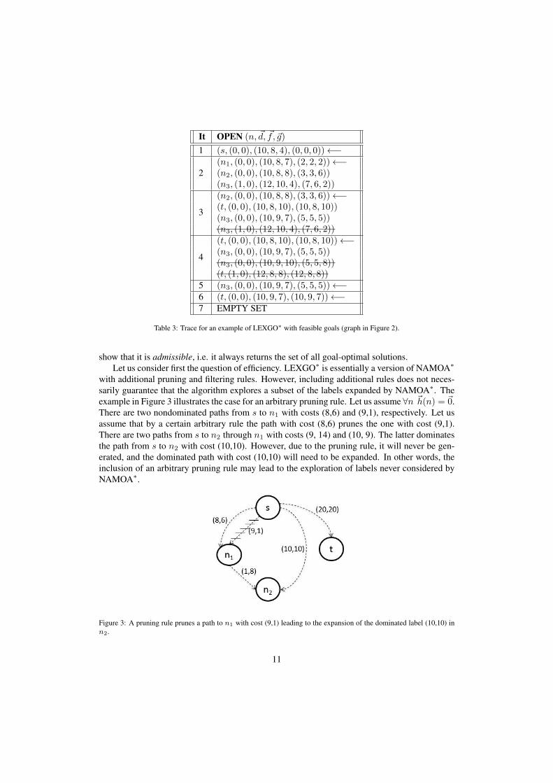
show that it is admissible, i.e. it always returns the set of all goal-optimal solutions.Let us consider first the question of efficiency. LEXGO∗ is essentially a version of NAMOA∗

with additional pruning and filtering rules. However, including additional rules does not neces-sarily guarantee that the algorithm explores a subset of the labels expanded by NAMOA∗. Theexample in Figure 3 illustrates the case for an arbitrary pruning rule. Let us assume ∀n ~h(n) = ~0.There are two nondominated paths from s to n1 with costs (8,6) and (9,1), respectively. Let usassume that by a certain arbitrary rule the path with cost (8,6) prunes the one with cost (9,1).There are two paths from s to n2 through n1 with costs (9, 14) and (10, 9). The latter dominatesthe path from s to n2 with cost (10,10). However, due to the pruning rule, it will never be gen-erated, and the dominated path with cost (10,10) will need to be expanded. In other words, theinclusion of an arbitrary pruning rule may lead to the exploration of labels never considered byNAMOA∗.

Figure 3: A pruning rule prunes a path to n1 with cost (9,1) leading to the expansion of the dominated label (10,10) inn2.

11

So we must formally show that the additional rules of LEXGO∗ guarantee that only a subsetof the labels expanded by NAMOA∗ are actually considered. To do so, Lemma 1 analyzes therelation between pruning, goal, and Pareto preferences. Then, Theorem 1 proves the desiredefficiency of LEXGO∗, and finally, Theorem 2 establishes its admissibility.

Lemma 1. Assume ~ε � ~0. Thena) If ~y ≺P ~y′ then ~y + ~ε ≺G ~y′ + ~ε.b) If ~y ≺P ~y′ then ~y + ~ε ≺P ~y′ + ~ε.c) If ~y ≺P ~y′ and ~y′ ≺ ~y′′, then ~y ≺P ~y′′.

Proof. Notice that, by definition,

δi(~y, ~y′) = 0 ⇒ ∀k ∈ Ii sk ≥ s′k (15)

Additionally, assume di(~y) = di(~y′). Since ~y has greater or equal slack than ~y′ for all goalsin level i, then it is straightforward that,

∀~ε � ~0, di(~y′ + ~ε) ≥ di(~y + ~ε) (16)

Notice again that, by definition,

δj(~y, ~y′) < dj(~y′)− dj(~y) ⇒ ∀~ε � ~0, dj(~y′ + ~ε) > dj(~y + ~ε) (17)

Property (a) follows then from the definition of goal preferences. Assume ~y ≺P ~y′, and that∃j dj(~y) < dj(~y′)∧(∀i < j di(~y) = di(~y′)). Then, from equations 16 anf 17, ~y′+~ε will nothave better deviation over ~y+~ε for any of the first j levels, and will have strictly worse deviationfor at least one of them, i.e. ~y + ~ε ≺G ~y′ + ~ε.

For part (b) we still have to prove the additional constraints imposed on cross-slacks. Let usdenote by s′′k and s′′′k the slack for goal k of vectors ~y + ~ε and ~y′ + ~ε respectively. For all levelsi < j we have,

δi(~y, ~y′) = 0 ⇒ ∀k ∈ Ii sk ≥ s′k ⇒ ∀k ∈ Ii s′′k ≥ s′′′k ⇒ δi(~y + ~ε, ~y′ + ~ε) = 0

and also di(~y′ + ~ε) ≥ di(~y + ~ε).If for some m < j dm(~y′ + ~ε) > dm(~y + ~ε), then δm(~y + ~ε, ~y′ + ~ε) = 0 < dm(~y′ + ~ε) −

dm(~y + ~ε), and the property holds. Otherwise, we need to prove that the condition on cross-slacks still holds for level j. Let us define δi(~y, ~y′) = wi ×max(0, s′i − si). The following is analternate definition of formula 8,

δj(~y, ~y′) =∑m∈Ij

δm(~y, ~y′)

Analogously, let us define di(~y) = wi ×max(0, yi − ti). Then,

dj(~y) =∑m∈Ij

dm(~y)

Now, we analyze for each goal m ∈ Ij its influence in deviations and cross-slack. We havethree cases to consider,

12

• When sm = s′m, deviations increase in the same amount (i.e. their relative difference doesnot change) and δm(~y + ~ε, ~y′ + ~ε) = δm(~y, ~y′) = 0.

• If sm > s′m, then dm(~y′)− dm(~y) ≤ dm(~y′ + ~ε)− dm(~y + ~ε), i.e. the relative differencebetween deviations can never decrease. Since δm(~y, ~y′) = δm(~y+~ε, ~y′+~ε) , the conditionwill hold for the goal.

• If sm < s′m, then we have to consider three distinct cases,

– When 0 ≤ εm ≤ sm < s′m, both deviations are zero, their relative difference remainszero and δm(~y, ~y′) does not change.

– When sm < εm ≤ s′m, we have [dm(~y′)−dm(~y)]−[dm(~y′+~ε)−dm(~y+~ε)] = wm×(εm−sm). However, we also have δm(~y, ~y′)−δm(~y+~ε, ~y′+~ε) = wm×(εm−sm),i.e. it decreases in the same amount as before, and the inequality still holds for goalm.

– When sm < s′m < εm, we have [dm(~y′) − dm(~y)] − [dm(~y′ + ε) − dm(~y + ε)] =

wm × (s′m − sm). However, δm(~y, ~y′)− δm(~y +~ε, ~y′ +~ε) = wm × (s′m − sm), i.e.it also decreases in the same amount as before, and the inequality still holds for goalm.

Part (c) is quite straightforward. Notice that,

~y′ ≺ ~y′′ ⇒ ∀l∀k ∈ Il s′k ≥ s′′k (18)

If ~y ≺P ~y′, then we have that for all levels i < j, δi(~y, ~y′) = 0, δi(~y, ~y′′) = 0, and di( ~y′′) ≥di(~y′) = di(~y).

Let us examine level j. From equation 18 it follows that δj(~y, ~y′) ≥ δj(~y, ~y′′) and fromdominance dj( ~y′′) ≥ dj(~y′). In consequence,

dj( ~y′′)− dj(~y) ≥ dj(~y′)− dj(~y) > δj(~y, ~y′) ≥ δj(~y, ~y′′) (19)

and therefore ~y ≺P ~y′′.

Theorem 1. When the lower bound function is monotone LEXGO∗ explores a subset of the la-bels explored by NAMOA∗, i.e. if NAMOA∗ does not explore a label (n,~g), LEXGO∗ will notexplore it either.

Proof. A label (n,~g, ~f) is not explored by NAMOA∗ if: (a) ∃~c∗ ∈ C∗ such that ~c∗ ≺ ~f , or (b)~g is dominated in n.

It is quite straightforward that LEXGO∗ never explores a label discarded by NAMOA∗ bycondition (a). Since C∗G ⊆ C∗, for all c∗ ∈ C∗, either c∗ ∈ C∗G, or ~dB = ~d∗ ≺L ~d(~c∗). In thelatter case, if for some ~f , ~c∗ ≺ ~f , then ~d∗ ≺L ~d(~c∗) �L ~d(~f). Therefore, LEXGO∗ filters thelabels with equations 13 and 14.

Let us consider now labels discarded by NAMOA∗ by condition (b). Let us assume a non-dominated path P = (s, n, . . . , ni, . . . , nk) to nk represented by label (nk, ~g, ~f), and its twosubpaths P1 = (s, n, . . . , ni) and P2 = (ni+1, . . . , nk). Let us also assume a dominated pathP ′ = (s, . . . , nk) to nk in OPEN with label (nk, ~g′, ~f ′). Finally, lets assume that P1 is the largestsubpath of P to enter OPEN, with label (ni, ~g1, ~f1). This situation is depicted in Figure 4.

13

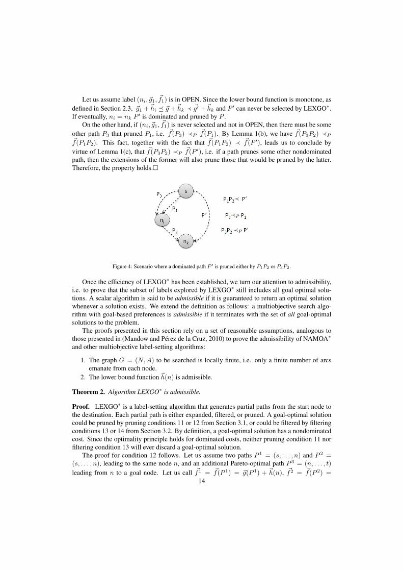
Let us assume label (ni, ~g1, ~f1) is in OPEN. Since the lower bound function is monotone, asdefined in Section 2.3, ~g1 + ~hi � ~g + ~hk ≺ ~g′ + ~hk and P ′ can never be selected by LEXGO∗.If eventually, ni = nk P

′ is dominated and pruned by P .On the other hand, if (ni, ~g1, ~f1) is never selected and not in OPEN, then there must be some

other path P3 that pruned P1, i.e. ~f(P3) ≺P ~f(P1). By Lemma 1(b), we have ~f(P3P2) ≺P~f(P1P2). This fact, together with the fact that ~f(P1P2) ≺ ~f(P ′), leads us to conclude byvirtue of Lemma 1(c), that ~f(P3P2) ≺P ~f(P ′), i.e. if a path prunes some other nondominatedpath, then the extensions of the former will also prune those that would be pruned by the latter.Therefore, the property holds.�

Figure 4: Scenario where a dominated path P ′ is pruned either by P1P2 or P3P2.

Once the efficiency of LEXGO∗ has been established, we turn our attention to admissibility,i.e. to prove that the subset of labels explored by LEXGO∗ still includes all goal optimal solu-tions. A scalar algorithm is said to be admissible if it is guaranteed to return an optimal solutionwhenever a solution exists. We extend the definition as follows: a multiobjective search algo-rithm with goal-based preferences is admissible if it terminates with the set of all goal-optimalsolutions to the problem.

The proofs presented in this section rely on a set of reasonable assumptions, analogous tothose presented in (Mandow and Pérez de la Cruz, 2010) to prove the admissibility of NAMOA∗

and other multiobjective label-setting algorithms:

1. The graph G = (N,A) to be searched is locally finite, i.e. only a finite number of arcsemanate from each node.

2. The lower bound function ~h(n) is admissible.

Theorem 2. Algorithm LEXGO∗ is admissible.

Proof. LEXGO∗ is a label-setting algorithm that generates partial paths from the start node tothe destination. Each partial path is either expanded, filtered, or pruned. A goal-optimal solutioncould be pruned by pruning conditions 11 or 12 from Section 3.1, or could be filtered by filteringconditions 13 or 14 from Section 3.2. By definition, a goal-optimal solution has a nondominatedcost. Since the optimality principle holds for dominated costs, neither pruning condition 11 norfiltering condition 13 will ever discard a goal-optimal solution.

The proof for condition 12 follows. Let us assume two paths P 1 = (s, . . . , n) and P 2 =(s, . . . , n), leading to the same node n, and an additional Pareto-optimal path P 3 = (n, . . . , t)

leading from n to a goal node. Let us call ~f1 = ~f(P 1) = ~g(P 1) + ~h(n), ~f2 = ~f(P 2) =14

~g(P 2) + ~h(n). Since the lower bound is optimistic, we know that ~h(n) � ~g(P 3). Let uscall ~e = ~g(P 3) − ~h(n) � ~0. Extending P 1 and P 2 with P 3, the costs of both solutions arerespectively ~f13 = ~g(P 1) +~g(P 3) = ~g(P 1) +~h(n) +~e = ~f1 +~e and ~f23 = ~g(P 2) +~g(P 3) =

~g(P 2) + ~h(n) + ~e = ~f2 + ~e.Let us assume that P 1 prunes P 2 in virtue of condition 12. Then ~f1 ≺P ~f2 and, by Lemma

1(a), ~f13 = ~f1 + ~e ≺G ~f2 + ~e = ~f23, so by this expansion P 2 does not lead to a better solutionthan P 1. Since no assumptions were made about P 3, the result holds for every expansion of n,therefore P 2 does not lead to a better solution than P 1 and the pruning is correct.

Finally, let us consider filtering condition 14, due to the lexicographic selection policy, thedeviation of the first solution found ~dB = ~dt is trivially equal or lexicographically better thanthe deviation of any other label in OPEN. No goal-optimal solution cost ~c∗ ∈ C∗G with deviation~d(~c∗) can have worse lexicographical deviation than ~dB Therefore, filtering condition 14 neverfilters goal-optimal solutions.

Since LEXGO* never prunes nor filters goal-optimal solutions, the only remaining possibilityis that they are all selected and found before termination, i.e. LEXGO∗ is admissible.�

5. Experiments

In this work we aim to improve over the efficiency of full multiobjective search, concentratingsearch effort on a subset of all Pareto optimal solutions. Algorithm LEXGO∗ uses lexicographicgoals to characterize this subset. This section analyzes the relative space and time performanceof LEXGO∗, versus a search of the full Pareto set of solutions based on NAMOA∗ that calculatesfirst the full Pareto set, and then determines the subset of goal-optimal solutions from it.

Moreover, we analyze the performance of LEXGO∗ with progressively stricter goals. On oneextreme, when all nondominated solutions satisfy all goals, LEXGO∗ will return the full Paretoset. At the opposite, it will return only the subset that minimizes deviation from unsatisfied goals.

In our experiments we use randomly generated grids which are a standard testbed in theevaluation of multicriteria search algorithms (Machuca et al., 2012) (Raith and Ehrgott, 2009).In particular, we generate square bidimensional grids of 100 × 100 nodes with a vicinity offour neighbors. The start node is placed at the grid’s center (50, 50). A single destination nodeis placed in the diagonal from the center to the bottom right corner. Different solution depthsare considered, varying from 20 to 100, i.e. for solution depth d, the destination node is atcoordinates (50+d/2, 50+d/2). A set of five different problems was generated for each solutiondepth. For each arc, three integer scalar costs ~c(i, j) = (c1, c2, c3) were randomly generated inthe range [1,10] using an uniform distribution, i.e. leading to uncorrelated objectives.

All the experiments were carried out considering three goals grouped in two priority levels,

Level 1 g1 ≤ t1, w1 = 0.5. g2 ≤ t2, w2 = 0.5

Level 2 g3 ≤ t3, w3 = 1

We define sets of target values for each problem in terms of the ideal ~α = (α1, α2, α3), andnadir points ~β = (β1, β2, β3). These were previously calculated from the full Pareto sets ob-tained with NAMOA∗. The nadir point is generally unknown in practice, but we take advantageof it in these experiments to obtain targets with different degrees of satisfaction for the purposeof experimentation. In a practical situation the ideal point is known thanks to the lower bound

15

Execution time (s) % to NAMOA∗ Labels explored % to NAMOA∗

NAMOA∗ 5369.6 100% 2550354 100%LEXGO∗

(k1 = 1) 5411.5 100.8% 2550347 99.9%(k1 = 0.75) 4569.9 85.1% 2473138 96.9%(k1 = 0.5) 1073.6 20% 1512099 59.2%(k1 = 0.25) 35.4 0.7% 216826 8.5%(k1 = 0) 0.1 0.001% 1994 0.08%

Table 4: Relative performance of LEXGO∗ over NAMOA∗ for d = 100 in Class I problems.

precalculations (Tung and Chew, 1992). These also provide the nadir point for two objectives,and at least an approximation for three or more objectives.

Three different classes of experiments were carried out. For the first class, five different targetsets were calculated as follows,

ti = αi + (βi − αi)× k1, k1 ∈ {0, 0.25, 0.5, 0.75, 1} (20)

For example, for k1 = 1 all Pareto optimal solutions will satisfy all goals, and for k1 = 0 noPareto solution will likely satisfy them.

For the second class, targets of the first level were fixed for k1 = 0.5, which was found toprovide satisfactory solutions. We then measured efficiency setting stricter targets for the thirdgoal,

t3 = α3 + (β3 − α3)× k2 k2 = k1 × k′, where k′ ∈ {0.25, 0.5, 0.75, 1} (21)

These values of t3 allow us to evaluate the performance when some goals are satisfied andsome not. Finally, the performance of LEXGO∗ was evaluated with and without the pruningcondition defined in equation 12, in order to evaluate its overall effectiveness.

The algorithms were implemented in Common Lisp using LispWorks Professional 6.01 (64-bit), and run on a 3GHz Intel Xeon X5472 with 32 Gb of RAM, under Windows Server 2008 R2(64-bit). The algorithms were implemented to share as much code as possible. Lexicographicorder was used to choose among nondominated open alternatives in NAMOA∗, and to break tiesin LEXGO∗. In all cases we used the lower bound function proposed by Tung and Chew (Tungand Chew, 1992).

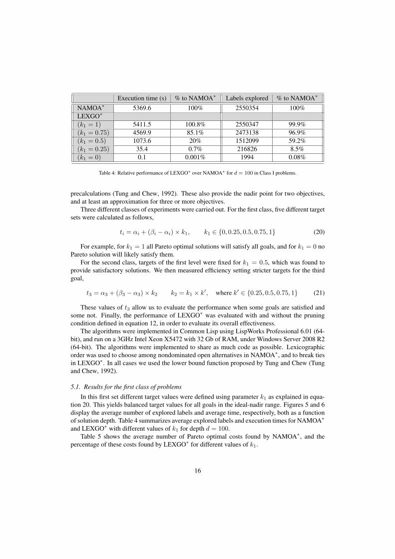
5.1. Results for the first class of problems

In this first set different target values were defined using parameter k1 as explained in equa-tion 20. This yields balanced target values for all goals in the ideal-nadir range. Figures 5 and 6display the average number of explored labels and average time, respectively, both as a functionof solution depth. Table 4 summarizes average explored labels and execution times for NAMOA∗

and LEXGO∗ with different values of k1 for depth d = 100.Table 5 shows the average number of Pareto optimal costs found by NAMOA∗, and the

percentage of these costs found by LEXGO∗ for different values of k1.

16

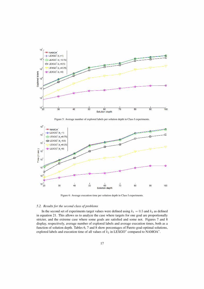
Figure 5: Average number of explored labels per solution depth in Class I experiments.

Figure 6: Average execution time per solution depth in Class I experiments.

5.2. Results for the second class of problems

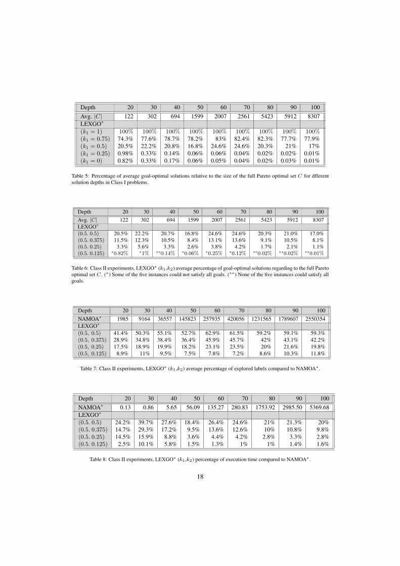
In the second set of experiments target values were defined using k1 = 0.5 and k2 as definedin equation 21. This allows us to analyze the case where targets for one goal are proportionallystricter, and the extreme case where some goals are satisfied and some not. Figures 7 and 8display, respectively, average number of explored labels and average execution times, both as afunction of solution depth. Tables 6, 7 and 8 show percentages of Pareto goal-optimal solutions,explored labels and execution time of all values of k2 in LEXGO∗ compared to NAMOA∗.

17

Depth 20 30 40 50 60 70 80 90 100Avg. |C| 122 302 694 1599 2007 2561 5423 5912 8307LEXGO∗

(k1 = 1) 100% 100% 100% 100% 100% 100% 100% 100% 100%(k1 = 0.75) 74.3% 77.6% 78.7% 78.2% 83% 82.4% 82.3% 77.7% 77.9%(k1 = 0.5) 20.5% 22.2% 20.8% 16.8% 24.6% 24.6% 20.3% 21% 17%(k1 = 0.25) 0.98% 0.33% 0.14% 0.06% 0.06% 0.04% 0.02% 0.02% 0.01%(k1 = 0) 0.82% 0.33% 0.17% 0.06% 0.05% 0.04% 0.02% 0.03% 0.01%

Table 5: Percentage of average goal-optimal solutions relative to the size of the full Pareto optimal set C for dfferentsolution depths in Class I problems.

Depth 20 30 40 50 60 70 80 90 100Avg. |C| 122 302 694 1599 2007 2561 5423 5912 8307LEXGO∗

(0.5. 0.5) 20.5% 22.2% 20.7% 16.8% 24.6% 24.6% 20.3% 21.0% 17.0%(0.5. 0.375) 11.5% 12.3% 10.5% 8.4% 13.1% 13.6% 9.1% 10.5% 8.1%(0.5. 0.25) 3.3% 5.6% 3.3% 2.6% 3.8% 4.2% 1.7% 2.1% 1.1%(0.5. 0.125) ∗0.82% ∗1% ∗∗0.14% ∗0.06% ∗0.25% ∗0.12% ∗∗0.02% ∗∗0.02% ∗∗0.01%

Table 6: Class II experiments, LEXGO∗ (k1,k2) average percentage of goal-optimal solutions regarding to the full Paretooptimal set C. (∗) Some of the five instances could not satisfy all goals. (∗∗) None of the five instances could satisfy allgoals.

Depth 20 30 40 50 60 70 80 90 100NAMOA∗ 1985 9164 36557 145823 257935 420056 1231565 1789607 2550354LEXGO∗

(0.5, 0.5) 41.4% 50.3% 55.1% 52.7% 62.9% 61.5% 59.2% 59.1% 59.3%(0.5, 0.375) 28.9% 34.8% 38.4% 36.4% 45.9% 45.7% 42% 43.1% 42.2%(0.5, 0.25) 17.5% 18.9% 19.9% 18.2% 23.1% 23.5% 20% 21.6% 19.8%(0.5, 0.125) 8.9% 11% 9.5% 7.5% 7.8% 7.2% 8.6% 10.3% 11.8%

Table 7: Class II experiments, LEXGO∗ (k1,k2) average percentage of explored labels compared to NAMOA∗.

Depth 20 30 40 50 60 70 80 90 100NAMOA∗ 0.13 0.86 5.65 56.09 135.27 280.83 1753.92 2985.50 5369.68LEXGO∗

(0.5. 0.5) 24.2% 39.7% 27.6% 18.4% 26.4% 24.6% 21% 21.3% 20%(0.5. 0.375) 14.7% 29.3% 17.2% 9.5% 13.6% 12.6% 10% 10.8% 9.8%(0.5. 0.25) 14.5% 15.9% 8.8% 3.6% 4.4% 4.2% 2.8% 3.3% 2.8%(0.5. 0.125) 2.5% 10.1% 5.8% 1.5% 1.3% 1% 1% 1.4% 1.6%

Table 8: Class II experiments, LEXGO∗ (k1,k2) percentage of execution time compared to NAMOA∗.

18

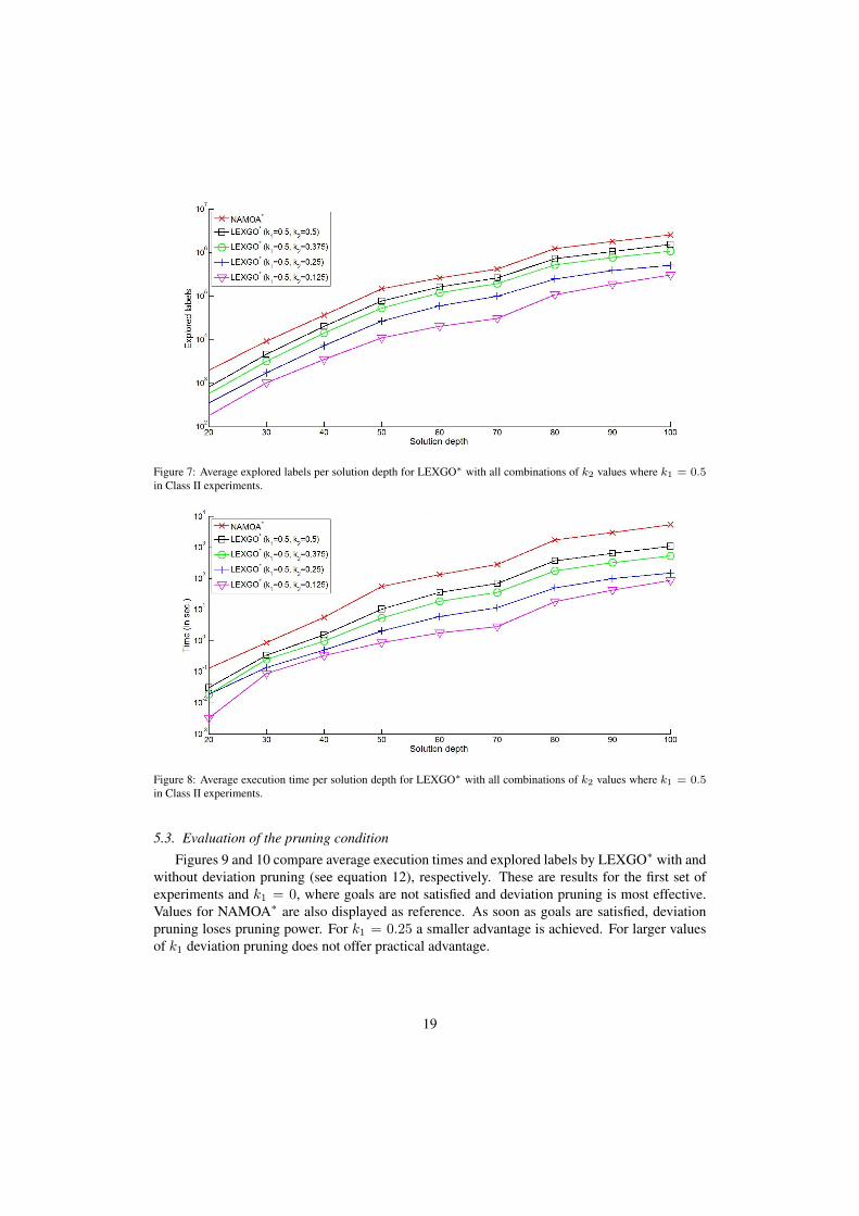
Figure 7: Average explored labels per solution depth for LEXGO∗ with all combinations of k2 values where k1 = 0.5in Class II experiments.

Figure 8: Average execution time per solution depth for LEXGO∗ with all combinations of k2 values where k1 = 0.5in Class II experiments.

5.3. Evaluation of the pruning condition

Figures 9 and 10 compare average execution times and explored labels by LEXGO∗ with andwithout deviation pruning (see equation 12), respectively. These are results for the first set ofexperiments and k1 = 0, where goals are not satisfied and deviation pruning is most effective.Values for NAMOA∗ are also displayed as reference. As soon as goals are satisfied, deviationpruning loses pruning power. For k1 = 0.25 a smaller advantage is achieved. For larger valuesof k1 deviation pruning does not offer practical advantage.

19

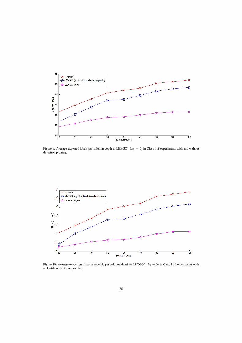
Figure 9: Average explored labels per solution depth to LEXGO∗ (k1 = 0) in Class I of experiments with and withoutdeviation pruning.

Figure 10: Average execution times in seconds per solution depth to LEXGO∗ (k1 = 0) in Class I of experiments withand without deviation pruning.

20

6. Discussion

Regarding Class I problems, a small time overhead can be observed for LEXGO∗ with k1 = 1when compared with NAMOA∗. In this case both algorithms return exactly the same set ofsolutions, and perform virtually the same number of label expansions. The time difference canbe attributed to the extra calculations of deviation from targets needed by LEXGO∗ for all costlabels, and the extra checks for pruning and filtering that do not provide any advantage in thissituation.

However, for other values of k1 LEXGO∗ achieves important reductions in time of almostone order of magnitude for k1 = 0.5, two orders of magnitude for k1 = 0.25, and up to fourorders of magnitude for k1 = 0. These are explained in large part by the reduction observed inthe number of labels selected, i.e. half the number of labels for k1 = 0.5, around one order ofmagnitude less for k1 = 0.25 and three orders of magnitude less for k1 = 0.

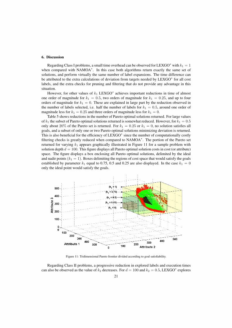
Table 5 shows reductions in the number of Pareto optimal solutions returned. For large valuesof k1 the subset of Pareto optimal solutions returned is somewhat reduced. However, for k1 = 0.5only about 20% of the Pareto set is returned. For k1 = 0.25 or k1 = 0, no solution satisfies allgoals, and a subset of only one or two Pareto optimal solutions minimizing deviation is returned.This is also beneficial for the efficiency of LEXGO∗ since the number of computationally costlyfiltering checks is greatly reduced when compared to NAMOA∗. The portion of the Pareto setreturned for varying k1 appears graphically illustrated in Figure 11 for a sample problem withsolution depth d = 100. This figure displays all Pareto optimal solution costs in cost (or attribute)space. The figure displays a box enclosing all Pareto optimal solutions, delimited by the idealand nadir points (k1 = 1). Boxes delimiting the regions of cost space that would satisfy the goalsestablished by parameter k1 equal to 0.75, 0.5 and 0.25 are also displayed. In the case k1 = 0only the ideal point would satisfy the goals.

Figure 11: Tridimensional Pareto frontier divided according to goal satisfiability.

Regarding Class II problems, a progressive reduction in explored labels and execution timescan also be observed as the value of k2 decreases. For d = 100 and k2 = 0.5, LEXGO∗ explores

21

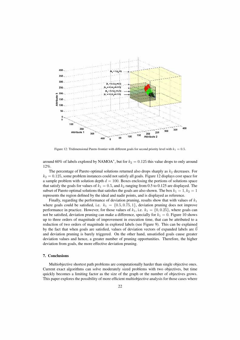
Figure 12: Tridimensional Pareto frontier with different goals for second priority level with k1 = 0.5.

around 60% of labels explored by NAMOA∗, but for k2 = 0.125 this value drops to only around12%.

The percentage of Pareto optimal solutions returned also drops sharply as k2 decreases. Fork2 = 0.125, some problem instances could not satisfy all goals. Figure 12 displays cost space fora sample problem with solution depth d = 100. Boxes enclosing the portions of solutions spacethat satisfy the goals for values of k1 = 0.5, and k2 ranging from 0.5 to 0.125 are displayed. Thesubset of Pareto optimal solutions that satisfies the goals are also shown. The box k1 = 1, k2 = 1represents the region defined by the ideal and nadir points, and is displayed as reference.

Finally, regarding the performance of deviation pruning, results show that with values of k1where goals could be satisfied, i.e. k1 = {0.5, 0.75, 1}, deviation pruning does not improveperformance in practice. However, for those values of k1, i.e. k1 = {0, 0.25}, where goals cannot be satisfied, deviation pruning can make a difference, specially for k1 = 0. Figure 10 showsup to three orders of magnitude of improvement in execution time, that can be attributed to areduction of two orders of magnitude in explored labels (see Figure 9). This can be explainedby the fact that when goals are satisfied, values of deviation vectors of expanded labels are ~0and deviation pruning is barely triggered. On the other hand, unsatisfied goals cause greaterdeviation values and hence, a greater number of pruning opportunities. Therefore, the higherdeviation from goals, the more effective deviation pruning.

7. Conclusions

Multiobjective shortest path problems are computationally harder than single objective ones.Current exact algorithms can solve moderately sized problems with two objectives, but timequickly becomes a limiting factor as the size of the graph or the number of objectives grows.This paper explores the possibility of more efficient multiobjective analysis for those cases where

22

the interesting portion of the Pareto front can be initially bounded. In practice, the efficientcalculation of cost estimates described by Tung and Chew provides important information aboutthe problem to be searched. In particular, the ideal point and at least an estimate of the nadirpoint are known before actual multiobjective search takes place.

We introduce LEXGO∗, a new algorithm that returns the subset of the Pareto front definedby a set of lexicographic goal preferences. We define goal-optimal solutions as the subset ofPareto-optimal solutions that satisfy all goals or, when these cannot be satisfied, the subset ofPareto-optimal solutions that minimize deviation from the goals. Under reasonable assumptionsthe algorithm is formally guaranteed to return the set of goal-optimal solutions, and to explore asubset of the labels explored by NAMOA∗, the state-of-the-art multiobjective search algorithm.The algorithm is evaluated over a set of standard multiobjective problems with three objectives.As goals become more restrictive, results show a dramatic reduction of up to several orders ofmagnitude in the number of explored labels and execution time. In general, the improvement inperformance is related to the reduction in the number of explored labels. However, in problemswere goals are not satisfied, the special pruning condition developed for LEXGO∗ can also havea fundamental influence in time performance.

In cases where the interesting portion of the Pareto front can be bounded, LEXGO∗ can bean algorithm of choice to reduce execution time from hours to seconds, or to explore hardermultiobjective problems.

Acknowledgments

This work is partially funded by Consejería de Innovación, Ciencia y Empresa. Junta deAndalucía (España), P07-TIC-03018, and Gobierno de España, Plan Nacional de I+D+i, grantTIN2009-14179.

References

Chankong, V., Haimes, Y., 1983. Multiobjective Decision Making: Theory and Methodology. North-Holland.Clímaco, J. C. N., Craveirinha, J. M. F., Pascoal, M. M. B., 2003. A bicriterion approach for routing problems in

multimedia networks. Networks 41 (4), 206–220.Dasgupta, P., Chakrabarti, P., DeSarkar, S., 1999. Multiobjective Heuristic Search. Vieweg, Braunschweig/Wiesbaden.Delle Fave, F., Canu, S., Iocchi, L., Nardi, D., Ziparo, V., 2009. Multi-objective multi-robot surveillance. In: 4th Inter-

national Conference on Autonomous Robots and Agents, 2009. ICARA 2009. pp. 68–73.Delling, D., Wagner, D., 2009. Pareto Paths with SHARC. In: Proceedings of the 8th International Symposium on

Experimental Algorithms (SEA’09). Vol. 2. Springer Verlag, pp. 125–136.Fujimura, K., 1996. Path planning with multiple objectives. Robotics Automation Magazine, IEEE 3 (1), 33–38.Gabrel, V., Vanderpooten, D., 2002. Enumeration and interactive selection of efficient paths in a multiple criteria graph

for scheduling an earth observing satellite. European Journal of Operational Research 139 (3), 533–542.Galand, L., Perny, P., 2006. Search for compromise solutions in multiobjective state space graphs. In: ECAI. pp. 93–97.Hansen, P., 1979. Bicriterion path problems. In: Lecture Notes in Economics and Mathematical Systems 177. Springer,

pp. 109–127.Jozefowiez, N., Semet, F., Talbi, E.-G., 2008. Multi-objective vehicle routing problems. European Journal of Operational

Research 189, 293–309.Machuca, E., Mandow, L., 2012. Multiobjective heuristic search in road maps. Expert Syst. Appl. 39 (7), 6435–6445.Machuca, E., Mandow, L., Pérez de la Cruz, J. L., 2009. An evaluation of heuristic functions for bicriterion shortest

path problems. In: Seabra Lopes, L., Lau, N., Mariano, P., Rocha, L. (Eds.), New Trends in Artificial Intelligence.Proceedings of EPIA’09. Universidade de Aveiro, Portugal, pp. 205–216.

Machuca, E., Mandow, L., Pérez de la Cruz, J. L., Ruiz-Sepulveda, A., 2012. A comparison of heuristic best-firstalgorithms for bicriterion shortest path problems. European Journal of Operational Research 217 (1), 44 – 53.

23

Mali, G., Michail, P., Zaroliagis, C., 2012. Faster multiobjective heuristic search in road maps. In: Proc. Int. Conf. onAdvances in Information and Communication Technologies - ICT 2012. Vol. 3. pp. 67–72.

Mandow, L., Pérez de la Cruz, J. L., 2001. A heuristic search algorithm with lexicographic goals. Engineering Applica-tions of Artificial Intelligence 14 (6), 751 – 762.

Mandow, L., Pérez de la Cruz, J. L., 2009. A memory-efficient search strategy for multiobjective shortest path problems.KI 2009: Advances in Artificial Intelligence 5803, 25–32.

Mandow, L., Pérez de la Cruz, J. L., 2010. Multiobjective A* search with consistent heuristics. Journal of the ACM57 (5), 27:1–25.

Martins, E. Q. V., 1984. On a multicriteria shortest path problem. European Journal of Operational Research 16 (2),236–245.

Müller-Hannemann, M., Weihe, K., 2006. On the cardinality of the Pareto set in bicriteria shortest path problems. Annalsof Operations Research 147 (1), 269–286.

Pearl, J., 1984. Heuristics. Addison-Wesley, Reading, Massachusetts.Pérez de la Cruz, J.L., Mandow, L., Machuca, E. (2013). A Case of Pathology in Multiobjective Heuristic Search. Journal

of Artificial Intelligence Research, Volume 48, 717–732Raith, A., Ehrgott, M., Apr. 2009. A comparison of solution strategies for biobjective shortest path problems. Computers

& Operations Research 36 (4), 1299–1331.Romero, C., 1991. Handbook of critical issues in goal programming. Pergamon Press.Sanders, P., Mandow, L., 2013. Parallel label-setting multi-objective shortest path search. In: 27th IEEE International

Parallel and Distributed Processing Symposium (IPDPS 2013), 215–224.Stewart, B. S., White, C. C., 1991. Multiobjective A*. Journal of the ACM 38 (4), 775–814.Tamiz, M., Jones, D. F., El-Darzi, E., Jan. 1995. A review of Goal Programming and its applications. Annals of Opera-

tions Research 58 (1), 39–53.Tung, C. T., Chew, K. L., 1992. A multicriteria Pareto-optimal path algorithm. European Journal of Operational Research

62, 203–209.

24