Multimodel assessment of water scarcity underclimate changeJacob Schewea,1, Jens Heinkea,b, Dieter Gertena, Ingjerd Haddelandc, Nigel W. Arnelld, Douglas B. Clarke,Rutger Dankersf, Stephanie Eisnerg, Balázs M. Feketeh, Felipe J. Colón-Gonzálezi, Simon N. Goslingj, Hyungjun Kimk,Xingcai Liul, Yoshimitsu Masakim, Felix T. Portmannn,o, Yusuke Satohp, Tobias Stackeq, Qiuhong Tangl,Yoshihide Wadar, Dominik Wissers, Torsten Albrechta, Katja Frielera, Franziska Pionteka, Lila Warszawskia,and Pavel Kabatt,u

aPotsdam Institute for Climate Impact Research, 14412 Potsdam, Germany; bInternational Livestock Research Institute, Nairobi, Kenya; cNorwegian WaterResources and Energy Directorate, N-0301 Oslo, Norway; dWalker Institute for Climate System Research, University of Reading, Reading RG6 6AR, UnitedKingdom; eCentre for Ecology and Hydrology, Wallingford OX10 8BB, United Kingdom; fMet Office Hadley Centre, Exeter EX1 3PB, United Kingdom; gCenterfor Environmental Systems Research, University of Kassel, 34109 Kassel, Germany; hCivil Engineering Department, The City College of New York, New York,NY 10031; iAbdus Salam International Centre for Theoretical Physics, I-34151Trieste, Italy; jSchool of Geography, University of Nottingham, Nottingham NG72RD, United Kingdom; kInstitute of Industrial Science , The University of Tokyo, 4-6-1 Komaba, Meguro, Tokyo 153-8505, Japan; pDepartment of CivilEngineering, The University of Tokyo, 7-3-1 Hongo, Bunkyo, Tokyo 113-8654, Japan; lInstitute of Geographic Sciences and Natural Resources Research, ChineseAcademy of Sciences, Beijing 100101, China; mCenter for Global Environmental Research, National Institute for Environmental Studies, Tsukuba 305-8506,Japan; nLOEWE Biodiversity and Climate Research Centre and Senckenberg Research Institute and Natural History Museum, 60325 Frankfurt am Main,Germany; oInstitute of Physical Geography, Goethe University Frankfurt, 60438 Frankfurt am Main, Germany; qMax Planck Institute for Meteorology, 20146Hamburg, Germany; rDepartment of Physical Geography, Utrecht University, 3584 CS Utrecht, The Netherlands; sCenter for Development Research, Universityof Bonn, 53113 Bonn, Germany; tInternational Institute for Applied Systems Analysis, A-2361 Laxenburg, Austria; and uWageningen University and ResearchCentre, 6708, Wageningen, The Netherlands

Edited by Hans Joachim Schellnhuber, Potsdam Institute for Climate Impact Research, Potsdam, Germany, and approved August 13, 2013 (received for reviewJanuary 31, 2013)

Water scarcity severely impairs food security and economic pros-perity inmany countries today. Expected future population changeswill, in many countries as well as globally, increase the pressure onavailable water resources. On the supply side, renewable waterresources will be affected by projected changes in precipitationpatterns, temperature, and other climate variables. Here we usea large ensemble of global hydrological models (GHMs) forced byfive global climate models and the latest greenhouse-gas concen-tration scenarios (Representative Concentration Pathways) to syn-thesize the current knowledge about climate change impacts onwater resources. We show that climate change is likely to exacer-bate regional and global water scarcity considerably. In particular,the ensemble average projects that a global warming of 2 °C abovepresent (approximately 2.7 °C above preindustrial) will confront anadditional approximate 15% of the global population with a severedecrease in water resources and will increase the number of peopleliving under absolutewater scarcity (<500m3 per capita per year) byanother 40% (according to some models, more than 100%) com-pared with the effect of population growth alone. For some indica-tors of moderate impacts, the steepest increase is seen between thepresent day and 2 °C, whereas indicators of very severe impacts in-crease unabated beyond 2 °C. At the same time, the study highlightslargeuncertainties associatedwith these estimates,with bothglobalclimate models and GHMs contributing to the spread. GHM uncer-tainty is particularly dominant in many regions affected by decliningwater resources, suggesting a high potential for improved waterresource projections through hydrological model development.

climate impacts | hydrological modeling | Inter-Sectoral Impact ModelIntercomparison Project

Freshwater is one of the most vital natural resources of theplanet. The quantities that humans need for drinking and

sanitation are relatively small, and the fact that these basic needsare not satisfied for many people today is primarily a matter ofaccess to, and quality of, available water resources (1). Muchlarger quantities of water are required for many other purposes,most importantly irrigated agriculture, but also for industrial use,in particular for hydropower and the cooling of thermoelectricpower plants (2, 3). These activities critically depend on a suffi-cient amount of freshwater that can be withdrawn from rivers,lakes, and groundwater aquifers. Whereas scarcity of freshwater

resources already constrains development and societal well-beingin many countries (4, 5), the expected growth of global populationover the coming decades, together with growing economic pros-perity, will increase water demand and thus aggravate theseproblems (6–8).Climate change poses an additional threat to water security

because changes in precipitation and other climatic variablesmay lead to significant changes in water supply in many regions(6–11). The effect of climate change on water resources is,however, uncertain for a number of reasons. Climate modelprojections, although rather consistent in terms of global averagechanges, disagree on the magnitude, and in many cases even thesign, of change at a regional scale, in particular when it comes toprecipitation patterns (12). In addition, the way in which pre-cipitation changes translate into changes in hydrological varia-bles such as surface or subsurface runoff and river discharge (i.e.,runoff accumulated along the river network), and thus in re-newable water resources, depends on many biophysical charac-teristics of the affected region (e.g., orography, vegetation, andsoil properties) and is the subject of hydrological models, whichrepresent a second level of uncertainty (11, 13).In the framework of the Inter-Sectoral Impact Model In-

tercomparison Project [ISI-MIP; Warszawski et al. (14) in thisissue of PNAS] a set of nine global hydrological models, oneglobal land-surface model, and one dynamic global vegetationmodel [here summarized as global hydrological models (GHMs);Materials and Methods] has been applied using bias-correctedforcing from five different global climate models (GCMs) underthe newly developed Representative Concentration Pathways(RCPs). The purpose is to explore the associated uncertaintiesand to synthesize the current state of knowledge about theimpact of climate change on renewable water resources atthe global scale. In this paper we investigate the multimodel

Author contributions: J.S., K.F., F.P., L.W., and P.K. designed research; J.S., J.H., D.G., I.H.,N.A., D.B.C., R.D., S.E., B.M.F., F.J.C.-G., S.N.G., H.K., X.L., Y.M., F.T.P., Y.S., T.S., Q.T., Y.W.,and D.W. performed research; J.S. and T.A. analyzed data; and J.S. wrote the paper.

The authors declare no conflict of interest.

This article is a PNAS Direct Submission.1To whom correspondence should be addressed. E-mail: jacob.schewe@pik-potsdam.de.

This article contains supporting information online at www.pnas.org/lookup/suppl/doi:10.1073/pnas.1222460110/-/DCSupplemental.

www.pnas.org/cgi/doi/10.1073/pnas.1222460110 PNAS | March 4, 2014 | vol. 111 | no. 9 | 3245–3250

SUST

AINABILITY

SCIENCE

SPEC

IALFEATU

RE

ensemble projections and the associated spread for changes inannual discharge—taken here as a first-order measure of thewater resources available to humans. We then reconcile thesehydrological changes with global population patterns to estimatehow many people will be living in areas affected by a givenchange in water resources. Finally, we apply a commonly usedmeasure of water scarcity to estimate the percentage of theworld’s population living in water-scarce countries and toquantify the contributions of both climate change and populationchange to the change in water scarcity. Results are presented asa function of global mean warming above the present day to ac-count for the relative independence of regional temperature,precipitation, and runoff changes of the rate of warming (15, 16)and to allow for systematic comparison of climate change impactsacross scenarios and sectors.

ResultsDischarge Trends and Uncertainties. We first consider the spatialpattern of relative change in annual mean discharge at 2 °Cglobal warming compared with present day (the term “presentday” in this study refers to the 1980–2010 average, which is ∼0.7 °C warmer globally than preindustrial), under RCP8.5 (Fig. 1).The multimodel mean across all GHMs and GCMs (Fig. 1,Upper) exhibits a number of robust large-scale features. In par-ticular, discharge is projected to increase at high northern lat-itudes, in eastern Africa and on the Indian peninsula, and todecrease in a number of regions including the Mediterraneanand large parts of North and South America. In these regions,

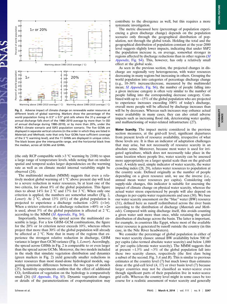
a relatively high level of agreement across the multimodel en-semble on the sign of change indicates high confidence. Most ofthese patterns are consistent with previous studies (8, 11, 17, 18),but there are also some differences. For example, ensemble pro-jections using the previous generation of GCMs and climate sce-narios found a robust runoff increase in southeastern SouthAmerica (19, 20), where we find no clear trend, or partly evena drying trend. Whereas those latter studies used larger GCMensembles, we apply an unprecedented number of GHMs as well asthe new RCP climate forcing. At 3 °C of global mean warming, thepattern of change is similar to that at 2 °C, although the changes areenhanced in many regions, and new robust trends emerge in someregions (most notably a strong negative trend in Mesoamerica; SIAppendix, Fig. S1).Inother parts of the globe, however, the projections are subject to

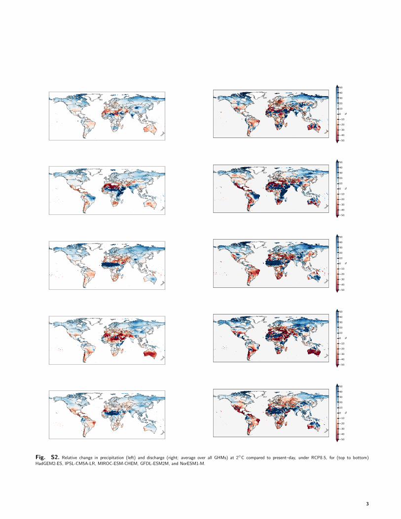
a large spread across the ensemble. In many regions, forcing bydifferent GCMs yields discharge changes (averaged across GHMs)that are large but of opposite sign (SI Appendix, Fig. S2 shows in-dividualmaps of precipitation anddischarge changes).Accordingly,the spread owing to differences betweenGCMs dominates the totalensemble spread in these regions (Fig. 1,Lower). By contrast, GHMspread is dominant in many regions that are subject to dischargereductions (e.g., northern and southern Africa). In most otherregions showing a large total spread, GHMs andGCMs contributeabout equally. Note that the bias correction applied to theGCMdata (Materials and Methods) substantially reduces the spreadamong the GCMs’ present-day climatologies, but not among theirfuture temperature and precipitation trends (21).

Population Affected by Severe Changes in Water Resources. To putthese discharge changes into a societal perspective, we reconcilethem with the spatial distribution of population, using pop-ulation projections from the newly developed Shared Socioeco-nomic Pathways (SSPs) (22). In the following, we will focus onthe middle-of-the-road population scenario according to SSP2,which projects global population to increase up to a peak ataround 10 billion by the year 2090 and includes substantialchanges in relative population densities among countries; con-stant present-day population will be considered additionally asa reference case.We first consider two criteria for a severe decrease in average

annual discharge, as an indicator of renewable water resources:a reduction by more than 20% and a reduction by more than 1SD (σ) of 1980–2010 annual discharge. Both criteria can be seenas first-order indicators of when available water resources con-sistently fall short of what a given population has adapted to andthus serious adaptation challenges are likely to arise. In manycases, a given discharge decrease may be detected using eithercriterion. In regions where interannual variability is high butbaseline discharge is low, the first criterion is particularly im-portant because even discharge reductions smaller than 1σ canaggravate water stress significantly in these regions. Conversely,in regions with low interannual variability, the second criteriondetects low-amplitude changes that may nonetheless requiresubstantial adaptation action as they transgress the range of pastvariability [e.g., in central and western Africa; Piontek et al. (23)in this issue of PNAS]. Based on grid-cell discharge averagedover 31-y periods that correspond to a given level of globalwarming, and on gridded population projections (Materials andMethods and SI Appendix, Table S1), we compute the percentageof global population living in countries with a discharge re-duction according to either or both of the criteria (Fig. 2). Withglobal mean warming on the horizontal axis, the differencesbetween the different RCPs in this population-weighted metric,as well as in globally averaged runoff, are small and in the rangeof interdecadal variability (SI Appendix, Fig. S3), meaning thatthese global, long-term indicators do not depend strongly on therate of global warming. We therefore concentrate on RCP8.5

Fig. 1. Relative change in annual discharge at 2 °C compared with presentday, under RCP8.5. (Upper) Color hues show the multimodel mean change,and saturation shows the agreement on the sign of change across all GHM–

GCM combinations (percentage of model runs agreeing on the sign; colorscheme following ref. 58). (Lower) Ratio of GCM variance to total variance;in red (blue) areas, GHM (GCM) variance predominates. GHM variance wascomputed across all GHMs for each GCM individually, and then averagedover all GCMs; vice versa for GCM variance. Greenland has been masked.

3246 | www.pnas.org/cgi/doi/10.1073/pnas.1222460110 Schewe et al.

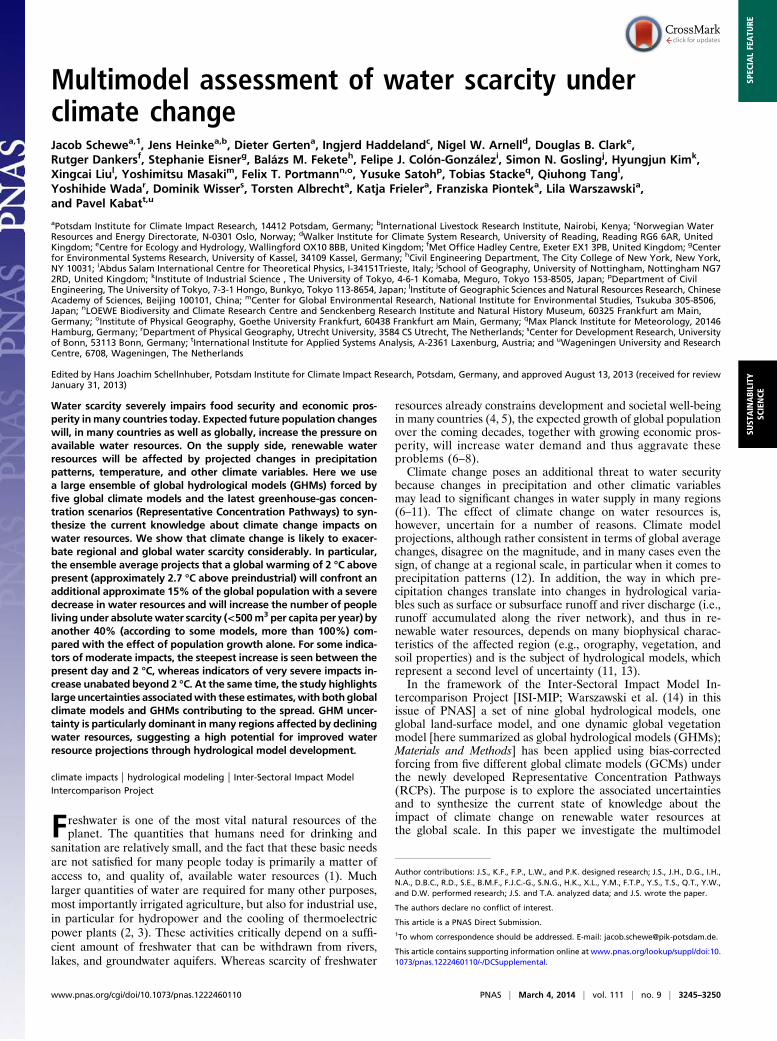
(the only RCP compatible with >3 °C warming by 2100) to spana large range of temperature levels, while noting that on smallerspatial and temporal scales larger dependencies on the warmingrate as well as on climate model internal variability might beobserved (24).The multimodel median (MMM) suggests that even a rela-

tively modest global warming of 1 °C above present day will leadto a severe reduction in water resources, by at least one of thetwo criteria, for about 8% of the global population. This figurerises to about 14% for 2 °C and 17% for 3 °C. When only onecriterion is applied, the numbers are somewhat smaller (Fig. 2,Lower): At 2 °C, about 13% (6%) of the global population isprojected to experience a discharge reduction >20% (>1σ).When a stricter criterion of a discharge reduction >40% or >2σis used, about 5% of the global population is affected at 2 °C,according to the MMM (SI Appendix, Fig. S4).Importantly, however, the spread across the multimodel en-

semble is large. For a few GHM–GCM combinations, the figurefor the 20% or 1σ criterion never exceeds 10%, whereas othersproject that more than 30% of the global population will alreadybe affected at 2 °C. Note that in many of the regions that ex-perience the strongest relative reduction in discharge, GHMvariance is larger than GCM variance (Fig. 1, Lower). Accordingly,the spread across GHMs in Fig. 2 is comparable to or even largerthan the spread across GCMs. Moreover, the two models includedin the study that simulate vegetation distribution and dynamics(green markers in Fig. 2) yield generally smaller reductions inwater resources than most stand-alone hydrological models, sug-gesting systematic differences between the two types of models(25). Sensitivity experiments confirm that the effect of additionalCO2 fertilization of vegetation on the hydrology is comparativelysmall (26) (SI Appendix, Fig. S5). Dynamic vegetation changesor details of the parameterizations of evapotranspiration may

contribute to the divergence as well, but this requires a moresystematic investigation.The metric discussed here (percentage of population experi-

encing a given discharge change) depends on the populationscenario only through the geographical distribution of pop-ulation, not through the global totals. Holding the total and thegeographical distribution of population constant at the year-2000level suggests slightly lower impacts, indicating that under SSP2the population increase is, on average, somewhat stronger inregions affected by discharge reductions than in other regions (SIAppendix, Fig. S4). This, however, has only a relatively smalleffect at the global scale.As seen in the previous section, the projected changes in dis-

charge are regionally very heterogeneous, with water resourcesdecreasing in many regions but increasing in others. Grouping theworld population into categories of percentage discharge change(e.g., 10–30% increase/decrease, measured by the multimodelmean; SI Appendix, Fig. S6), the number of people falling intoa given increase category is often very similar to the number ofpeople falling into the corresponding decrease category. Com-bined with up to ∼15% of the global population who are projectedto experience increases exceeding 100% of today’s discharge,overall more people will be affected by discharge increases thanwill be by decreases. Whereas such increases may enhance actualwater availability in many cases, they can also entail adverseimpacts such as increasing flood risk, deteriorating water quality,and malfunctioning of water-related infrastructure (27).

Water Scarcity. The impact metric considered in the previoussection measures, at the grid-cell level, significant departuresfrom present levels of resource availability, irrespective of whatthose levels are. It is thus an indicator of adaptation challengesthat may arise, but not necessarily of resource scarcity in anabsolute sense. Moreover, because most water is used for irri-gated agriculture, which does not necessarily take place in thesame location where people live, water scarcity can be assessedmore appropriately on a larger spatial scale than on the grid-celllevel. A widely used, simple indicator of water scarcity, the watercrowding index (28, 29), relates water resources to population atthe country scale. Defined originally as the number of peopledepending on a given resource unit, we use the inverse (i.e.,annual mean water resources per capita). Considering onlysupply-side changes, this indicator is suitable for assessing theimpact of climate change on physical water scarcity, whereas theactual water stress experienced by people will also depend onchanges in per-capita water requirements and uses (30). We baseour water scarcity assessment on the “blue” water (BW) resource(31), defined here as runoff redistributed across the river basinaccording to the distribution of discharge (Materials and Meth-ods). Compared with using discharge itself, this avoids countinga given water unit more than once, while retaining the spatialdistribution of discharge across the basin. The latter is important,for example, in countries like Egypt, where most of the availablewater resource is generated by runoff outside the country (in thiscase, in the Nile River headwaters).We consider the percentage of global population in either of

two water scarcity classes: annual BW availability below 500 m3

per capita (also termed absolute water scarcity) and below 1,000m3 per capita (chronic water scarcity). The MMM suggests thatat present ∼1.5% and ∼3% of the global population fall intothese two scarcity classes, respectively (the first class beinga subset of the second; Fig. 3 A and B). This is similar to previousestimates at the country level (7) but much lower than estimatesdone at the grid-cell level (4, 17) or river basin level (7) becauselarger countries may not be classified as water-scarce eventhough significant parts of their population live in water-scarcegrid cells. Whereas the country level might in some cases be toocoarse for a realistic assessment of water scarcity and generally

Fig. 2. Adverse impact of climate change on renewable water resources atdifferent levels of global warming. Markers show the percentage of theworld population living in 0.5° × 0.5° grid cells where the 31-y average ofannual discharge falls short of the 1980–2010 average by more than 1σ (SDof annual discharge during 1980–2010), or by more than 20%, under theRCP8.5 climate scenario and SSP2 population scenario. The five GCMs aredisplayed in separate vertical columns (in the order in which they are listed inMaterials and Methods; note that only four GCMs have sufficient coverageof the 3 °C warming level), and the 11 GHMs are displayed in unique colors.The black boxes give the interquartile range, and the horizontal black linesthe median, across all GCMs and GHMs.

Schewe et al. PNAS | March 4, 2014 | vol. 111 | no. 9 | 3247

SUST

AINABILITY

SCIENCE

SPEC

IALFEATU

RE

underestimate the global figure, the grid-cell level likely over-estimates it because water transfers between grid cells [and alsovirtual water imports related to trade of water-intensive goods(32)] are large in reality.Our present-day estimate is already subject to a significant

spread across the multimodel ensemble (ranging from 0 to 4% forthe<500 m3 class and 1–8% for the<1,000 m3 class), owing mainlyto differences in present-day discharge simulated by the differentGHMs (13). The present-day discharge estimates also depend toa certain extent on the observation-based dataset that was used forbias-correcting the climate input data (Materials and Methods).Under the SSP2 population scenario (and again using 31-y aver-ages associated with the different warming levels), the percentageof people living in countries below 500 m3 per capita (1,000 m3 percapita) is projected to rise to 6% (13%) at 1 °C, 9% (21%) at 2 °C,and 12% (24%) at 3 °C of global warming, according to the MMM(Fig. 3A andB). The high rates of rise between present-day and 1 °Ccould be partly related to the fact that the present-day estimate isvery low, and different spatial scales of analysis may lead to differentrelative changes.Population growth plays a major role in this increase in water

scarcity because it reduces per-capita availability even with un-changed resources. To separate the population signal from theclimate signal, we use each model combination’s average 1980–2010 discharge pattern to compute the percentage of people thatwould fall into a scarcity class if climate were to remain constantand population changed according to SSP2 (SI Appendix, Fig. S7).As found in previous studies (6, 31, 33), population change

explains the larger part of the overall change in water scarcity.Subtracting the constant-climate scenario from the full scenarioand dividing by the constant-climate scenario indicates by howmuch the level of water scarcity expected owing to populationchange alone is amplified by climate change (Fig. 3 C and D).According to the MMM, this amplification is nearly 40% for the<500 m3 class at 1 °C and 2 °C global warming. The factor issomewhat lower (approximately 25%) at 3 °C, indicating that atthis level of warming the effect of additional climate change onthis global metric becomes smaller compared with the effect ofpopulation changes. Note that this is partly related to the relativetiming of warming and population change: In an even faster-warming scenario than RCP8.5, a warming from 2 °C to 3 °Cmight still have a relatively larger impact because it would beassociated with generally lower population numbers. This ob-servation illustrates how climate change and population changecombine to aggravate global water scarcity: A country can movetoward the water scarcity threshold both through populationgrowth and through declining water resources, and depending onthe relative rates of change, it may be one or the other factor thateventually causes the threshold to be crossed.

Along similar lines, for the ≤1,000 m3 class, the MMM am-plification due to climate change is nearly 30% at 1 °C, drops toabout 20% at 2 °C, and is close to zero at 3 °C. A number ofmodel combinations yield negative values in Fig. 3 C and D; inthese cases, climate change is projected to alleviate the globalincrease in water-scarce population that is expected owing topopulation change. The GHMs projecting a positive effect ofclimate change on chronic water scarcity (i.e., yielding negativevalues in Fig. 3D) are primarily models that show a large numberof people in this scarcity class in the first place (yellow and redmarkers in Fig. 3B). This suggests that in these models manycountries in regions that get drier are already in this class atpresent, such that the potential for additional countries to moveinto the class is smaller compared with the potential for countriesto move out of the class in regions that get wetter.

DiscussionOur multimodel assessment adds to extensive previous work, inparticular in the framework of the European Union IntegratedProject Water and Global Change (EU-WATCH) and WaterModel Intercomparison Project (WaterMIP) (13), which dem-onstrated that hydrological models are a significant source ofuncertainty in projections of runoff and evapotranspiration (11).The present study, using a larger ensemble ensemble of GHMsand GCMs and the state-of-the-art RCP climate forcing avail-able from Coupled Model Intercomparison Project Phase 5(CMIP-5), explores the range of uncertainty not only in hydro-logical change but also in its effect on people. Results are mappedagainst global mean temperature increase to allow direct com-parison of the impacts at different levels of global warming.It is important to note that our globally aggregated water

scarcity estimates can obscure potentially much more severechanges at the scale of individual countries or locations. Forexample, if a number of countries were to move into a givenwater scarcity class, but at the same time other countries witha similar share of global population were to move out of thisclass, the resulting change on the global scale would be close tozero. Likewise, if the amplification of the global water scarcitysignal by climate change becomes small at higher levels ofwarming, as seen in Fig. 3 C and D, this could mean that climatechange continues to force additional countries into the scarcityclass, but at the same time other countries move out of the class(e.g., because of more pronounced regional precipitation increasesat this temperature level). The results in Fig. 3 must thus beinterpreted with care, and the numbers in Fig. 3 C and D inparticular are more likely to represent a lower bound to the cli-mate change contribution in regions that are affected by a dis-charge decrease. Moreover, changes within a given water scarcityclass are not detected here but can be very important. Countries

A B

DC

Fig. 3. Percentage of world population living incountries with annual mean BW availability (Materialsand Methods) below 500 m3 per capita (Left) andbelow 1,000 m3 per capita (Right). Symbols as in Fig. 2.(A and B) RCP8.5 climate scenario, population changeaccording to SSP2. (C and D) Amplification by climatechange of the level of water scarcity that is expectedfrom population change alone; computed as the dif-ference between a constant-climate scenario (SI Ap-pendix, Fig. S7) and the full scenario shown above,divided by the constant-climate scenario, and ex-pressed as percentage (so that the population-onlycase equals 100%). For example, in C, the MMMindicates that at 2 °C global warming, climate changeamplifies the level of absolute water scarcity (numberof people below 500 m3 per capita) expected frompopulation change alone by about 36%.

3248 | www.pnas.org/cgi/doi/10.1073/pnas.1222460110 Schewe et al.

that are already extremely water-scarce will be all the more vul-nerable to even small decreases in resource availability.Although the water crowding index is an appropriate measure

for supply-side effects on global water scarcity, it is not a mea-sure of the actual problems that countries and people face insatisfying their water needs because it does not take the demandside into account. Future water stress (as measured, for instance,by the ratio of water use to availability) will depend on changesin demand, for example, related to economic growth, lifestylechanges, or technological developments, as well as on watermanagement practices and infrastructure. Alternative sources ofwater for agriculture, such as “green” water contained in the soil(31, 33, 34), and nonrenewable water resources (35, 36), alsoaffect actual BW requirements.We have only considered long-term averages, neglecting po-

tential changes in the interannual and seasonal availability ofwater resources and their variability (10, 37). Changes in sea-sonality can have severe impacts even if the annual average isstable e.g., if irrigation water availability in the growing seasonchanges, or if flood hazard is affected by changes in snow-meltrunoff [Dankers et al. (38) in this issue of PNAS]. Again, in-frastructure such as dams and reservoirs can substantially alterthe timing of water resource availability (39). Moreover, hydro-logical changes can have consequences going far beyond theavailability of water resources for human uses, for instance, byaltering the occurrence of damaging extreme events like floodsand droughts [Prudhomme et al. (40) in this issue of PNAS],affecting aquatic and terrestrial ecosystems (41), and potentiallyinteracting with, and amplifying, climate change impacts in othersectors (42).

ConclusionsWe have synthesized results from 11 GHMs with forcing fromfive GCMs to provide an overview of the state of the art ofmodeling the impact of climate change on global water resour-ces. In all metrics considered, we find a considerable spreadacross the simulation ensemble. GHMs and GCMs contribute tosimilar extents to the spread in relative discharge changes glob-ally. When changes in water scarcity are considered, GHMspread is in fact larger than GCM spread. This finding suggeststhat, although climate model uncertainty remains an importantconcern, further impact model development promises majorimprovements in water scarcity projections.The multimodel mean projected changes in annual discharge

are spatially heterogenous. As the planet gets warmer, a risingshare of the world population will be affected by severe reduc-tions in water resources, measured as deviation from present-daydischarge in terms of either SD or percentage. However, a simi-lar fraction of the population will experience increases in averagedischarge, which could potentially improve water availability, butalso entail adverse effects.Our estimate of water scarcity at the country scale indicates

that climate change may substantially aggravate the water scar-city problem. Depending on the rates of both population changeand global warming, the level of water scarcity expected owing topopulation change alone is amplified by up to 40% owing toclimate change, according to the multimodel mean; some modelssuggest an amplification by more than 100%. This adds up tobetween 5% and 20% of global population likely exposed toabsolute water scarcity at 2 °C of global warming. For chronicwater scarcity, most adverse climate change impacts alreadyoccur between present day and 2 °C, whereas beyond this tem-perature positive and negative additional impacts of climatechange are of a similar magnitude (although they affect differentgroups of people and therefore cannot be offset against eachother). However, absolute water scarcity continues to be sub-stantially amplified by climate change on the global scale evenbeyond 2 °C. We conclude that the combination of unmitigated

climate change and further population growth will expose a sig-nificant fraction of the world population to chronic or absolutewater scarcity. This dwindling per-capita water availability islikely to pose major challenges for societies to adapt their wateruse and management.

Materials and MethodsModels and Data. The GHMs used in this study are the DBH (43), H08 (44),Mac-PDM.09 (45), MATSIRO (46), MPI-HM (47), PCR-GLOBWB (36), VIC (48),WaterGAP (49), and WBMplus (50) hydrological models, the JULES (51) land-surface model, and the LPJmL (52) dynamic global vegetation model; thelatter two also represent vegetation dynamics in addition to hydrologicalprocesses. SI Appendix, Table S2 gives further model details. Forcing datawere derived from climate projections with the HadGEM2-ES, IPSL-CM5A-LR,MIROC-ESM-CHEM, GFDL-ESM2M, and NorESM1-M GCMs under the RCPs(53), which were prepared for the CMIP-5 (54). All required climate variableshave been bias-corrected (55) toward an observation-based dataset (56)using a newly developed method (21) that builds on earlier approaches (57)but was specifically designed to preserve the long-term trends in tempera-ture and precipitation projections to facilitate climate change studies. GHMswere run without direct coupling to GCMs, so that potential feedbacks (e.g.,from GHM-simulated evapotranspiration on precipitation) were not repre-sented. Further details about the GHM simulations can be found in the ISI-MIPsimulation protocol available at http://www.isi-mip.org/. Country-level UnitedNations World Population Prospects (historical) and SSP (projections) pop-ulation data at a 5-y time step were obtained from the SSP Database at https://secure.iiasa.ac.at/web-apps/ene/SspDb and linearly interpolated to obtain an-nual values. A gridded population dataset was also used in which the NationalAeronautics and Space Administration GPWv3 y-2010 gridded populationdataset (http://sedac.ciesin.columbia.edu/data/collection/gpw-v3) was scaledup to match the SSP country totals (neglecting changes in population distri-bution within countries).

Temperature Axis. Global mean temperature is calculated from the GCM data(including ocean cells) and presented as the difference from the 1980–2010average. For each GCM and RCP, 31-y periods are selected whose averagetemperature corresponds to the different levels of global warming (SI Ap-pendix, Table S1; note that GFDL-ESM2M does not reach the 3 °C warminglevel). Population affected by discharge changes (Fig. 2) was calculated usingthe population distribution corresponding to the middle year of each in-dividual 31-y period (except for the baseline period 1980–2010, which wasassumed to correspond to year-2000 population). Water scarcity (Fig. 3) wascalculated annually, using annual population values, and then averagedover the 31-y periods; results for the 0 °C baseline were obtained from the“constant-climate” run, that is, using 1980–2010 average BW resources andannual population values (discussed in the following section).

Water Scarcity. For assessing country-scale water scarcity, we calculate theannual mean BW resource availability following ref. 31: The sum of annualmean runoff R in each river basin b is redistributed across the basinaccording to the relative distribution of discharge Q, yielding the BW re-source in each grid cell i:

BWi =RbQi

.XQi ,

where Σ is the sum over all grid cells in basin b. BW is then summed up overall grid cells within a country and divided by the country’s population toyield the water crowding index. Finally, for each year, the total number ofpeople living in countries that are below a given threshold of this index (500m3 or 1,000 m3 per capita) is calculated and divided by global population toyield the corresponding percentage of world population. Results are againaveraged over the 31-y periods that correspond to the different levels ofglobal warming shown in Fig. 3 A and B. For the climate change contributionshown in Fig. 3 C and D, the subtraction of, and division by, the results fromthe constant-climate run is done year by year, and the resulting percentageis averaged over the 31-y periods.

Ensemble Statistics. Statistics across the multimodel ensemble were computedafter the calculation of the respective metric. For instance, in Fig. 1 the relativechange in discharge was calculated for each model combination individuallybefore computing the multimodel mean, agreement, and variances.

ACKNOWLEDGMENTS. The authors acknowledge theWorld Climate ResearchProgramme’s Working Group on Coupled Modelling, which is responsible for

Schewe et al. PNAS | March 4, 2014 | vol. 111 | no. 9 | 3249

SUST

AINABILITY

SCIENCE

SPEC

IALFEATU

RE

the Coupled Model Intercomparison Project, and thank the climate modelinggroups for producing and making available their model output. J.S. wishes tothankA. Levermann for helpful discussions. This work has been conducted underthe framework of the Inter-Sectoral Impact Model Intercomparison Project (ISI-MIP). The ISI-MIP Fast Track project underlying this paper was funded by theGerman Federal Ministry of Education and Research with project funding refer-ence number 01LS1201A. R.D. was supported by the joint Department of Energyand Climate Change/Defra Met Office Hadley Centre Climate Programme(GA01101). F.J.C.-G. was jointly funded by the European Union Seventh Frame-work Programme Quantifying Weather and Climate Impacts on health in

developing countries and HEALTHY FUTURES projects. S.N.G. was supportedby a Science, Technology and Society Priority Group grant from University ofNottingham. Y.M. was supported by the Environment Research and TechnologyDevelopment Fund (S-10) of the Ministry of the Environment, Japan. F.T.P. re-ceived funding from the European Union’s Seventh Framework Programme(FP7/2007-2013) under Grant 266992. K.F. was supported by the Federal Ministryfor the Environment, Nature Conservation and Nuclear Safety, Germany(11_II_093_Global_A_SIDS and LDCs). H.K. and Y.S. were jointly supported byJapan Society for the Promotion of Science KAKENHI (23226012) and Ministryof Education, Culture, Sports, Science and Technology SOUSEI Program.

1. Ohlsson L, Turton AR (1999) The turning of a screw: Social resource scarcity as a bot-tleneck in adaptation to water scarcity. Occasional Paper Series, School of Orientaland African Studies Water Study Group, University of London.

2. Wallace J (2000) Increasing agricultural water use efficiency to meet future foodproduction. Agric Ecosyst Environ 82(1-3):105–119.

3. Kummu M, Ward PJ, de Moel H, Varis O (2010) Is physical water scarcity a new phe-nomenon? Global assessment of water shortage over the last two millennia. EnvironRes Lett 5(3):034006.

4. Oki T, et al. (2001) Global assessment of current water resources using total runoffintegrating pathways. Hydrol Sci J 46(6):983–995.

5. Rijsberman F (2006) Water scarcity: Fact or fiction? Agric Water Manage 80:5–22.6. Vörösmarty CJ, Green P, Salisbury J, Lammers RB (2000) Global water resources:

Vulnerability from climate change and population growth. Science 289(5477):284–288.

7. Arnell NW (2004) Climate change and global water resources: SRES emissions andsocio-economic scenarios. Glob Environ Change 14(3-4):31–52.

8. Alcamo J, Flörke M, Märker M (2007) Future long-term changes in global water re-sources driven by socio-economic and climatic changes. Hydrol Sci J 52(3):247–275.

9. Milly PCD, Dunne KA, Vecchia AV (2005) Global pattern of trends in streamflow andwater availability in a changing climate. Nature 438(7066):347–350.

10. Fung F, Lopez A, New M (2011) Water availability in +2C and +4C worlds. Philos TransSer A 369(1934):99–116.

11. Hagemann S, et al. (2012) Climate change impact on available water resources ob-tained using multiple global climate and hydrology models. Earth Syst Dynam Discuss3(3-4):1321–1345.

12. Meehl G, Stocker T, Collins W (2007) Global Climate Projections (Cambridge UnivPress, Cambridge, UK).

13. Haddeland I, et al. (2011) Multimodel estimate of the global terrestrial water balance:Setup and first results. J Hydrometeorol 12(5):869–884.

14. Warszawski L, et al. (2014) The Inter-Sectoral Impact Model Intercomparison Project(ISI–MIP): Project framework. Proc Natl Acad Sci USA 111:3228–3232.

15. Frieler K, Meinshausen M, Mengel M, Braun N, Hare W (2012) A scaling approach toprobabilistic assessment of regional climate change. J Clim 25(4):3117–3144.

16. Tang Q, Lettenmaier DP (2012) 21st century runoff sensitivities of major global riverbasins. Geophys Res Lett 39(3):L06403.

17. Arnell NW, van Vuuren DP, Isaac M (2011) The implications of climate policy for theimpacts of climate change on global water resources. Glob Environ Change 21(2):592–603.

18. Gosling SN, Bretherton D, Haines K, Arnell NW (2010) Global hydrology modellingand uncertainty: Running multiple ensembles with a campus grid. Philos Trans Ser A368(1926):4005–4021.

19. Bates B, Kundzewicz Z, Wu S, Palutikof J (2008) Climate change and water. Technicalpaper of the Intergovernmental Panel on Climate Change (IPCC Secretariat, Geneva).

20. Füssel H, Heinke J, Popp A, Gerten D (2012) Climate change and water supply. ClimateChange, Justice and Sustainability: Linking Climate and Development Policy (Springer,Dordrecht, The Netherlands), pp 19–32.

21. Hempel S, Frieler K, Warszawski L, Schewe J, Piontek F (2013) A trend-preserving biascorrection the ISI-MIP approach. Earth System Dynamics 4(1):219–236.

22. Neill BCO, et al. (2012) Meeting report of the Workshop on the Nature and Use ofNew Socioeconomic Pathways for Climate Change Research, Boulder, CO, November2–4, 2011.

23. Piontek F, et al. (2014) Multisectoral climate impact hotspots in a warming world. ProcNatl Acad Sci USA 111:3233–3238.

24. Heinke J, et al. (2012) A new dataset for systematic assessments of climate changeimpacts as a function of global warming. Geoscientific Model Development Dis-cussions 5(4):3533–3572.

25. Davie JCS, et al. (2013) Comparing projections of future changes in runoff and waterresources from hydrological and ecosystem models in ISI-MIP. Earth System DynamicsDiscussions 4(1):279–315.

26. Piao S, et al. (2007) Changes in climate and land use have a larger direct impact thanrising CO2 on global river runoff trends. Proc Natl Acad Sci USA 104(39):15242–15247.

27. Kundzewicz ZW, et al. (2008) The implications of projected climate change forfreshwater resources and their management. Hydrol Sci J 53(1):3–10.

28. Falkenmark M, Lundqvist J, Widstrand C (1989) Macro-scale water scarcity requiresmicro-scale approaches. Aspects of vulnerability in semi-arid development. Nat Re-sour Forum 13(4):258–267.

29. Falkenmark M, et al. (2007) On the Verge of a New Water Scarcity (Stockholm In-ternational Water Institute, Stockholm).

30. Ashton PJ (2002) Avoiding conflicts over Africa’s water resources. Ambio 31(3):236–242.

31. Gerten D, et al. (2011) Global water availability and requirements for future foodproduction. J Hydrometeorol 12(5):885–899.

32. Hanasaki N, Inuzuka T, Kanae S, Oki T (2010) An estimation of global virtual waterflow and sources of water withdrawal for major crops and livestock products usinga global hydrological model. J Hydrol (Amst) 384(3-4):232–244.

33. Rockström J, et al. (2009) Future water availability for global food production: Thepotential of green water for increasing resilience to global change. Water Resour Res45:1–16.

34. Rost S, et al. (2008) Agricultural green and blue water consumption and its influenceon the global water system. Water Resour Res 44(9):1–17.

35. Taylor RG, et al. (2012) Ground water and climate change. Nature Climate Change 3:322–329.

36. Wada Y, et al. (2010) Global depletion of groundwater resources. Geophys Res Lett37(7):L20402.

37. Gosling SN, Taylor RG, Arnell NW, Todd MC (2011) A comparative analysis of pro-jected impacts of climate change on river runoff from global and catchment-scalehydrological models. Hydrol Earth Syst Sci 15(7):279–294.

38. Dankers et al. (2014) First look at changes in flood hazard in the Inter-SectoralImpact Model Intercomparison Project ensemble. Proc Natl Acad Sci USA 111:3257–3261.

39. Biemans H, et al. (2011) Impact of reservoirs on river discharge and irrigation watersupply during the 20th century. Water Resour Res 47(3):1–15.

40. Prudhomme et al. (2014) Hydrological droughts in the 21st century: Hotspots anduncertainties from a global multimodel ensemble experiment. Proc Natl Acad Sci USA111:3262–3267.

41. Gerten D, Schaphoff S, Lucht W (2007) Potential future changes in water limitationsof the terrestrial biosphere. Clim Change 80(3-4):277–299.

42. Parry M, et al. (2001) Millions at risk: Defining critical climate change threats andtargets. Glob Environ Change 11:181–183.

43. Tang Q, Oki T, Kanae S, Hu H (2007) The influence of precipitation variability andpartial irrigation within grid cells on a hydrological simulation. J Hydrometeorol 8:499–512.

44. Hanasaki N, et al. (2008) An integrated model for the assessment of global waterresources – Part 1: Model description and input meteorological forcing. Hydrol EarthSyst Sci 12(4):1007–1025.

45. Gosling SN, Arnell NW (2011) Simulating current global river runoff with a globalhydrological model: Model revisions, validation, and sensitivity analysis. Hydrol Pro-cesses 25:1129–1145.

46. Takata K, Emori S, Watanabe T (2003) Development of the minimal advancedtreatments of surface interaction and runoff. Global Planet Change 38(1-2):209–222.

47. Stacke T, Hagemann S (2012) Development and validation of a global dynamicalwetlands extent scheme. Hydrol Earth Syst Sci Discuss 9(1):405–440.

48. Liang X, Lettenmaier DP, Wood EF, Burges SJ (1994) A simple hydrologically basedmodel of land surface water and energy fluxes for general circulation models.J Geophys Res 99(D7):14415.

49. Döll P, Kaspar F, Lehner B (2003) A global hydrological model for deriving wateravailability indicators: model tuning and validation. J Hydrol (Amst) 270(1-2):105–134.

50. Wisser D, Fekete BM, Vörösmarty CJ, Schumann AH (2010) Reconstructing 20th cen-tury global hydrography: a contribution to the Global Terrestrial Network- Hydrology(GTN-H). Hydrol Earth Syst Sci 14(1):1–24.

51. Best MJ, et al. (2011) The Joint UK Land Environment Simulator (JULES), model de-scription Part 1: Energy and water fluxes. Geoscientific Model Development 4(3):677–699.

52. Bondeau A, et al. (2007) Modelling the role of agriculture for the 20th century globalterrestrial carbon balance. Glob Change Biol 13(3):679–706.

53. Moss RH, et al. (2010) The next generation of scenarios for climate change researchand assessment. Nature 463(7282):747–756.

54. Taylor KE, Stouffer RJ, Meehl GA (2012) An overview of CMIP5 and the experimentdesign. Bull Am Meteorol Soc 93:485–498.

55. Ehret U, Zehe E, Wulfmeyer V, Warrach-Sagi K, Liebert J (2012) HESS opinions: Shouldwe apply bias correction to global and regional climate model data? Hydrol Earth SystSci 16(9):3391–3404.

56. Weedon GP, et al. (2011) Creation of the WATCH forcing data and its use to assessglobal and regional reference crop evaporation over land during the twentiethcentury. J Hydrometeorol 12(5):823–848.

57. Hagemann S, et al. (2011) Impact of a statistical bias correction on the projectedhydrological changes obtained from three GCMs and two hydrology models. JHydrometeorol 12(4):556–578.

58. Kaye NR, Hartley A, Hemming D (2012) Mapping the climate: Guidance on appro-priate techniques to map climate variables and their uncertainty. GeoscientificModel Development 5(1):245–256.

3250 | www.pnas.org/cgi/doi/10.1073/pnas.1222460110 Schewe et al.

Multi-model assessment of water scarcity underclimate changeJacob Schewe ∗, Jens Heinke ∗ a, Dieter Gerten ∗ , Ingjerd Haddeland †, Nigel W. Arnell ‡, Douglas B. Clark §, Rutger Dankers¶, Stephanie Eisner ‖, Balazs Fekete ∗∗, Felipe J. Colon-Gonzalezb, Simon N. Gosling ††, Hyungjun Kim ‡‡, Xingcai Liu §§,Yoshimitsu Masaki ¶¶, Felix T. Portmann ∗∗∗, Yusuke Satoh †††, Tobias Stacke ‡‡‡, Qiuhong Tang §§ , Yoshihide Wada §§§,Dominik Wisserc, Torsten Albrecht ∗ , Katja Frieler ∗ , Franziska Piontek ∗ , Lila Warszawski ∗ , and Pavel Kabat ¶¶¶

∗Potsdam Institute for Climate Impact Research, Potsdam, Germany, aInternational Livestock Research Institute, Nairobi, Kenya,†Norwegian Water Resources and Energy

Directorate, Oslo, Norway,‡Walker Institute for Climate System Research, University of Reading, Reading, UK,§Centre for Ecology & Hydrology, Wallingford, UK,¶Met Office

Hadley Centre, Exeter, UK,‖Center for Environmental Systems Research (CESR), University of Kassel, Kassel, Germany,∗∗Civil Engineering Department, The City College of New

York, New York, USA, bAbdus Salam International Centre for Theoretical Physics, Trieste, Italy,††School of Geography, University of Nottingham, Nottingham, UK,‡‡Institute

of Industrial Science, The University of Tokyo, Tokyo, Japan,§§Institute of Geographic Sciences and Natural Resources Research, Chinese Academy of Sciences, Beijing,

China,¶¶Center for Global Environmental Research, National Institute for Environmental Studies, Tsukuba, Japan,∗∗∗Biodiversity and Climate Research Centre (LOEWE BiK-

F) & Senckenberg Research Institute and Natural History Museum, Frankfurt am Main, Germany; and Institute of Physical Geography, Goethe University Frankfurt, Frankfurt

am Main, Germany,†††Department of Civil Engineering, The University of Tokyo, Tokyo, Japan,‡‡‡Max Planck Institute for Meteorology, Hamburg, Germany,§§§Department

of Physical Geography, Utrecht University, Utrecht, Netherlands, cCenter for Development Research, University of Bonn, Bonn, Germany, and ¶¶¶International Institute for

Applied Systems Analysis, Laxenburg, Austria & Wageningen University and Research Centre, Wageningen, Netherlands

Supporting Information

1–2

<-50 -30 -10 10 30 >50relative change (%)

607080

agre

em

ent

(%)

Fig. S1. As Fig. 1 (upper panel) in the main text, but for a warming of 3◦C.

Table S1. Middle years of 31–year periods corresponding to the different levels of global warming(compared to present–day, i.e. the 1980–2010 average) in the individual GCMs under RCP8.5.Population projections for these same years were used, except at the 0◦C level which was assumedto correspond to year–2000 population

warming level HadGEM2-ES IPSL-CM5A-LR MIROC-ESM-CHEM GFDL-ESM2M NorESM1-M

0◦C 1995 1995 1995 1995 1995

1◦C 2021 2027 2023 2040 2035

2◦C 2044 2047 2043 2071 2062

3◦C 2062 2065 2061 - 2086∗

∗A 27–year period from 2073–2099 was used.

2

50

40

30

20

10

0

10

20

30

40

50

%

50

40

30

20

10

0

10

20

30

40

50

%

50

40

30

20

10

0

10

20

30

40

50

%

50

40

30

20

10

0

10

20

30

40

50

%

50

40

30

20

10

0

10

20

30

40

50

%

Fig. S2. Relative change in precipitation (left) and discharge (right; average over all GHMs) at 2◦C compared to present–day, under RCP8.5, for (top to bottom)

HadGEM2-ES, IPSL-CM5A-LR, MIROC-ESM-CHEM, GFDL-ESM2M, and NorESM1-M.

3

0.0 0.5 1.0 1.5 2.0 2.5 3.0 3.5Warming above 1980-2010 average ( ±C)

0.95

1.00

1.05

1.10

mm

/day

global meanrunoff

HadGEM2-ES

0.0 0.5 1.0 1.5 2.0 2.5 3.0 3.5Warming above 1980-2010 average ( ±C)

0

5

10

15

20

25

Perc

ent

of

worl

d p

opula

tion 1¾ or 20%

pop2000

HadGEM2-ES

0.0 0.5 1.0 1.5 2.0 2.5 3.0 3.5Warming above 1980-2010 average ( ±C)

0

5

10

15

20

25

Perc

ent

of

worl

d p

opula

tion 1¾ or 20%

SSP2

HadGEM2-ES

Fig. S3. Effect of different rates of global warming on global impact metrics. Shown are

results for one GCM (HadGEM2-ES), two GHMs (solid and dotted lines) and all four RCPs

(RCP2.6, dark blue; RCP4.5, turquoise; RCP6.0, orange; RCP8.5, red) at different levels of

global warming. Upper panel: Globally averaged runoff. Middle and lower panel: Same metric

as shown in Fig. 2 (upper panel) in the main paper. Middle panel: Assuming constant present–

day (2010) population. Lower panel: Assuming population change according to SSP2.

4

1 2 3Warming above 1980-2010 average (K)

0

5

10

15

20

25

30

35

40

Perc

ent

of

worl

d p

opula

tion

2¾ or 40%

1 2 3Warming above 1980-2010 average (K)

0

5

10

15

20

25

30

35

40

Perc

ent

of

worl

d p

opula

tion

1¾ or 20%

pop2000

Fig. S4. As upper panel of Fig. 2 in the main paper, but (upper panel) for a reduction by

more than 2σ or by more than 40%; and (lower panel) assuming constant year–2000 population.

1 2 3Warming above 1980-2010 average (K)

0

5

10

15

20

25

30

35

40

Perc

ent

of

worl

d p

opula

tion

1¾ or 20%

Fig. S5. As upper panel of Fig. 2 in the main paper, but with the quartiles and median

(shown by the black boxes) computed without the models that include vegetation dynamics

(JULES and LPJmL). The individual results of those models are highlighted in green colors,

where + denotes runs with varying atmospheric CO2 concentration, and ∼ denotes runs where

CO2 concentration has been varied according to historical values up until the year 2000, and

held constant at the year–2000 level thereafter.

5

1 2 3Warming above 1980-2010 average ( ±C)

0

20

40

60

80

100

Perc

ent

of

worl

d p

opula

tion

0

30

70

90

110

130

170

200

% o

f pre

sent-

day d

isch

arg

e

Fig. S6. Population affected by different levels of discharge increase or decrease. Shown

is the multi–model mean of the percentage of the world population living in grid cells where

31–year average discharge is a certain percentage of present–day (1980–2010) discharge, at

1◦C, 2◦C, and 3◦C of global warming, under RCP8.5 and SSP2.

0 1 2 3Warming above 1980-2010 average ( ◦ C)

0

5

10

15

20

25

30

Perc

ent

of

worl

d p

opula

tion

< 500m3

constClim + popSSP2

0 1 2 3Warming above 1980-2010 average ( ◦ C)

0

10

20

30

40

50

Perc

ent

of

worl

d p

opula

tion

< 1000m3

constClim + popSSP2

Fig. S7. As Fig. 3a and b in the main paper, but using a “Constant climate” scenario

(1980–2010 average discharge). SSP2 population data from the same years as in Fig. 3a and

b are used, relating the population time series to the temperature axis via the RCP8.5.

6

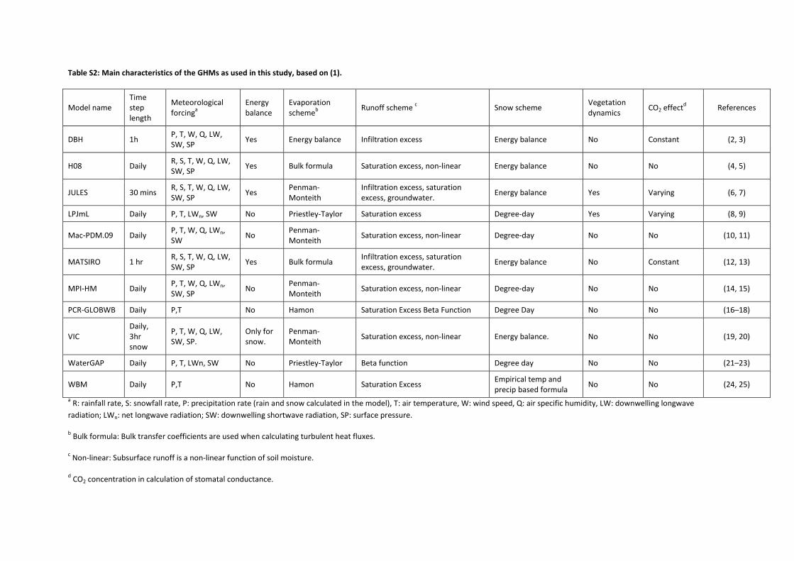
Table S2: Main characteristics of the GHMs as used in this study, based on (1).

Model name Time step length

Meteorological forcinga

Energy balance

Evaporation schemeb Runoff scheme c Snow scheme Vegetation

dynamics CO2 effectd References

DBH 1h P, T, W, Q, LW, SW, SP Yes Energy balance Infiltration excess Energy balance No Constant (2, 3)

H08 Daily R, S, T, W, Q, LW, SW, SP Yes Bulk formula Saturation excess, non-linear Energy balance No No (4, 5)

JULES 30 mins R, S, T, W, Q, LW, SW, SP Yes Penman-

Monteith Infiltration excess, saturation excess, groundwater. Energy balance Yes Varying (6, 7)

LPJmL Daily P, T, LWn, SW No Priestley-Taylor Saturation excess Degree-day Yes Varying (8, 9)

Mac-PDM.09 Daily P, T, W, Q, LWn, SW No Penman-

Monteith Saturation excess, non-linear Degree-day No No (10, 11)

MATSIRO 1 hr R, S, T, W, Q, LW, SW, SP Yes Bulk formula Infiltration excess, saturation

excess, groundwater. Energy balance No Constant (12, 13)

MPI-HM Daily P, T, W, Q, LWn, SW, SP No Penman-

Monteith Saturation excess, non-linear Degree-day No No (14, 15)

PCR-GLOBWB Daily P,T No Hamon Saturation Excess Beta Function Degree Day No No (16–18)

VIC Daily, 3hr snow

P, T, W, Q, LW, SW, SP.

Only for snow.

Penman-Monteith Saturation excess, non-linear Energy balance. No No (19, 20)

WaterGAP Daily P, T, LWn, SW No Priestley-Taylor Beta function Degree day No No (21–23)

WBM Daily P,T No Hamon Saturation Excess Empirical temp and precip based formula No No (24, 25)

a R: rainfall rate, S: snowfall rate, P: precipitation rate (rain and snow calculated in the model), T: air temperature, W: wind speed, Q: air specific humidity, LW: downwelling longwave radiation; LWn: net longwave radiation; SW: downwelling shortwave radiation, SP: surface pressure.

b Bulk formula: Bulk transfer coefficients are used when calculating turbulent heat fluxes.

c Non-linear: Subsurface runoff is a non-linear function of soil moisture.

d CO2 concentration in calculation of stomatal conductance.

Supplementary References

1. Haddeland I et al. (2011) Multimodel Estimate of the Global Terrestrial Water Balance: Setup and First Results. Journal of Hydrometeorology 12:869–884.

2. Tang Q, Oki T, Kanae S, Hu H (2007) The Influence of Precipitation Variability and Partial Irrigation within Grid Cells on a Hydrological Simulation. Journal of Hydrometeorology 8:499–512.

3. Tang Q, Oki T, Kanae S, Hu H (2008) Hydrological Cycles Change in the Yellow River Basin during the Last Half of the Twentieth Century. Journal of Climate 21:1790–1806.

4. Hanasaki N et al. (2008) An integrated model for the assessment of global water resources – Part 1: Model description and input meteorological forcing. Hydrology and Earth System Sciences 12:1007–1025.

5. Hanasaki N et al. (2008) An integrated model for the assessment of global water resources – Part 2: Applications and assessments. Hydrology and Earth System Sciences 12:1027–1037.

6. Best MJ et al. (2011) The Joint UK Land Environment Simulator (JULES), model description – Part 1: Energy and water fluxes. Geoscientific Model Development 4:677–699.

7. Clark DB et al. (2011) The Joint UK Land Environment Simulator (JULES), Model description – Part 2: Carbon fluxes and vegetation. Geoscientific Model Development Discussions.

8. Bondeau A et al. (2007) Modelling the role of agriculture for the 20th century global terrestrial carbon balance. Global Change Biology 13:679–706.

9. Rost S et al. (2008) Agricultural green and blue water consumption and its influence on the global water system. Water Resources Research 44:1–17.

10. Arnell N. (1999) A simple water balance model for the simulation of streamflow over a large geographic domain. Journal of Hydrology 217:314–335.

11. Gosling SN, Arnell NW (2011) Simulating current global river runoff with a global hydrological model: model revisions, validation, and sensitivity analysis. Hydrological Processes 25:1129–1145.

12. Takata K, Emori S, Watanabe T (2003) Development of the minimal advanced treatments of surface interaction and runoff. Global and Planetary Change 38:209–222.

13. Pokhrel Y et al. (2012) Incorporating Anthropogenic Water Regulation Modules into a Land Surface Model. Journal of Hydrometeorology 13:255–269.

14. Hagemann S, Dümenil Gates L (2003) Improving a subgrid runoff parameterization scheme for climate models by the use of high resolution data derived from satellite observations. Climate Dynamics 21:349–359.

15. Stacke T, Hagemann S (2012) Development and validation of a global dynamical wetlands extent scheme. Hydrology and Earth System Sciences Discussions 9:405–440.

16. Wada Y et al. (2010) Global depletion of groundwater resources. Geophysical Research Letters 37:L20402.

17. Van Beek LPH, Wada Y, Bierkens MFP (2011) Global monthly water stress: 1. Water balance and water availability. Water Resources Research 47:W07517.

18. Wada Y et al. (2011) Global monthly water stress: 2. Water demand and severity of water stress. Water Resources Research 47:W07518.

19. Liang X, Lettenmaier DP, Wood EF, Burges SJ (1994) A simple hydrologically based model of land surface water and energy fluxes for general circulation models. Journal of Geophysical Research 99:14415.

20. Lohmann D, Raschke E (1998) Regional scale hydrology: I. Formulation of the VIC-2L model coupled to a routing model. Hydrological Sciences Journal 43:131–141.

21. Döll P et al. (2012) Impact of water withdrawals from groundwater and surface water on continental water storage variations. Journal of Geodynamics 59–60:143–156.

22. Döll P, Kaspar F, Lehner B (2003) A global hydrological model for deriving water availability indicators: model tuning and validation. Journal of Hydrology 270:105–134.

23. Flörke M et al. (2013) Domestic and industrial water uses of the past 60 years as a mirror of socio-economic development: A global simulation study. Global Environmental Change 23:144–156.

24. Vörösmarty CJ, Federer CA, Schloss AL (1998) Potential evaporation functions compared on US watersheds: Possible implications for global-scale water balance and terrestrial ecosystem modeling. Journal of Hydrology 207:147–169.

25. Wisser D, Fekete BM, Vörösmarty CJ, Schumann AH (2010) Reconstructing 20th century global hydrography: a contribution to the Global Terrestrial Network- Hydrology (GTN-H). Hydrology and Earth System Sciences 14:1–24.