Multimineral Modeling - PTTC Rockiespttc.mines.edu/MM_Slides.pdf · 2015-07-07 · Multimineral...

$: Multimineral Modeling - PTTC Rockiespttc.mines.edu/MM_Slides.pdf · 2015-07-07 · Multimineral modeling solves for volumetric fractions and defines bulk mineralogy, Rhoma, PHIT;$
HIGHER STANDARDS

Multimineral Modeling Wesley Ingram [email protected]

1. Multimineral modeling using various datasets

2. Initial 2-phase model using core scanning data

3. Element to mineral and volumetric multimineral model

4. Calibrating models with lab data and core plug selection

© Weatherford Laboratories. All Rights Reserved. 2

Outline


Multimineral modeling

Multimineral modeling solves for volumetric fractions and defines bulk mineralogy, Rhoma, PHIT; often PHIE with CBW

Petrophysics solves for (Rhoma)a mineralogy using logs

Deterministic, probabilistic and hybrid methods are available

Deterministic solutions solve for 3-4 mineral phases, i.e. Vclay, Rhoma, PHIT, PHIE, CBW; probabilistic can be more

With lab data or core scanning techniques, similar models can be generated independently of logs


Traditional log-based methods

Apparent Mineral Matrix

Several multimineral solvers i.e., 3-phases, DEN-NEUT-PEF

Vertical axis = Rhoma (ρmaa)

Horizontal axis = Uma (Umaa)

Umaa = (Pe*ρb) – (φND*Ufl) / (1-φND)

ρmaa = ρb - (φND*ρfl) / (1-φND)


Geochemistry multimineral modeling

Defines matrix mineralogy from either minerals (XRD) and/or elements (XRF/ICP)

Determination from a physical rock sample

Thus, no need to correct for porosity or fluids and can go directly at Rhoma

The summation of mineral components multiplied by respective density, organic content is measured

weight volume

Proprietary Image

X-ray fluorescence (XRF) core scanning – 1-inch scale

Dual Energy CT (DECT) core scanning – sub-mm scale

Essentially high-res logs: XRF up to 30 elements; DECT Pef and Rhob

Non-destructive core analysis

XRF Scanner

CT Scanner

Post-slab Pre-slab






Outline


Mode Inputs

I. Spectral gamma

II. K, U and Th curves

III. DECT Rhob

IV. DECT Pef

Calibrated Model

• XRD & Clay Type

• TOC & Pyrolysis

• Rock Properties

DECT Model – Pre Slab

Model Outputs

I. Volume Clay

II. Volume Kerogen

III. Volume Calcite

IV. Volume Quartz

V. PHIT, CBW & PHIE

• Careful!! w/ porosity est.

• Clay typing for CBW & PHIE

• Vdolomite w/ neutron log

On right – organic-rich mudstone

Calculate U Index, cross-plot against kerogen values

TOC = 0.83(S1+S2)/10 + S4/10

S4 = (10TOC – (S1+S2))/10

Wk = 0.83(S2)/10 + S4/10

Convert Wk to Vk

Vk = (ρma)/(ρk)

ρk = ~1.15 to 1.9 g/cc


Example U-Ker validation

y = -0.9707x2 + 5.3491x + 0.9645 R² = 0.6033

1

10

0.1 1

Uranium-Organic Matrix

Uranium Index

Org

anic

Mat

rix

Proprietary Image

Solve for Vclay using the K & Th curve from spectral

GRcl = (P*Klog) + (T*Thlog) - i.e. U-stripped GR curve

VCL = ((GRcl(log) – GRcl(min))/(GRcl(max) – GRcl(min)))*(CL) - Linear

P = ~16; T = ~4 (~coefficients) CL = ~0.6 (Bhuyan and Passey, 1994)

With coefficients, calibrate to total clay, by formation or XRD

GR index is originally for shale, 0.6 is an estimation for clay


Solve for VCL before minerals


Adjusting the K-Th coefficients

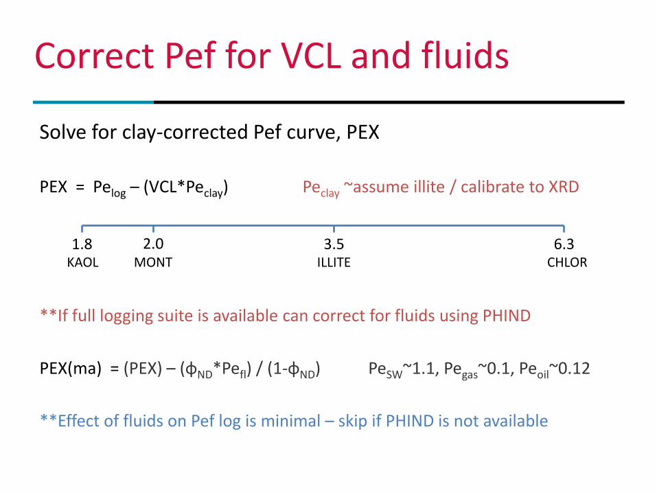
Solve for clay-corrected Pef curve, PEX

PEX = Pelog – (VCL*Peclay) Peclay ~assume illite / calibrate to XRD

**If full logging suite is available can correct for fluids using PHIND

PEX(ma) = (PEX) – (φND*Pefl) / (1-φND) PeSW~1.1, Pegas~0.1, Peoil~0.12

**Effect of fluids on Pef log is minimal – skip if PHIND is not available


Correct Pef for VCL and fluids

1.8 2.0 3.5 6.3 KAOL MONT ILLITE CHLOR

Remaining Pef response if from solid-phase minerals (Quartz-Calcite)

PEX(ma) = (Pequartz*Vquartz) + (Pecalcite*Vcalcite) - still 2 unknown volumes

PEX(ma) = (Pequartz*Vquartz) + Pecalcite*(1.00 – Vquartz) - rearrange for Vquartz

Vquartz = ((Pecalcite – PEX(ma)(log))/(Pecalcite – Pequartz))*(1.00 – VCL – Vker)

Vquartz = ((5.08 – PEX(ma)(log))/(5.08 – 1.81)*(1.00 – VCL – Vker)


2-phase mineral solution from Pef

1.81 5.08 Quartz Calcite

Quartz index Material balance


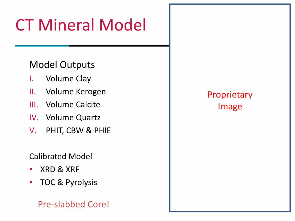
Model Outputs

I. Volume Clay

II. Volume Kerogen

III. Volume Calcite

IV. Volume Quartz

V. PHIT, CBW & PHIE

Calibrated Model

• XRD & XRF

• TOC & Pyrolysis

CT Mineral Model

Pre-slabbed Core!

Proprietary Image






Outline


Mode Inputs

I. XRF Major Elements

II. Traces included

III. EM Model high res

IV. CT Rhob

Calibrated Model

• XRD & Clay Type

• TOC & Pyrolysis

• Rock Properties

Multimineral Model – Post Slab

Model Outputs

I. Volume 6 to 8 minerals

II. More for the ambitious

III. Volume Kerogen

IV. PHIT, CBW & PHIE

• Validate kerogen here as well

• Clay typing for CBW & PHIE

• Much more accurate Rhomma

Element to Mineral Modeling involves numerous approaches the goals is to build representative model by formation

1. Straight stoichiometric approach can be used, i.e. XRF Ca is converted to CaCO3, Si is converted to SiO2….. And so on

2. Probabilistic approach can be used with elements or oxides to then generate minerals with the lowest residuals

3. Deterministic approach uses stoichiometric index curves, matched to lab-quality XRD data – essentially calibrated

4. Most important – avoid over solutions or too many minerals!


EM Model – high-res with XRF


Vca

Pore Volume

Vqrtz VCL

0.2 0.3 0.3

Solid

-ph

ase Rh

om

aa 1.0

0

0.05

Organic Matrix

Vdol

0.3

Best estimate for mix of minerals

Group Heavy Min FeS, CaPOF

Vorganics & Vhm weight to volume quite different

0.05

Vhm


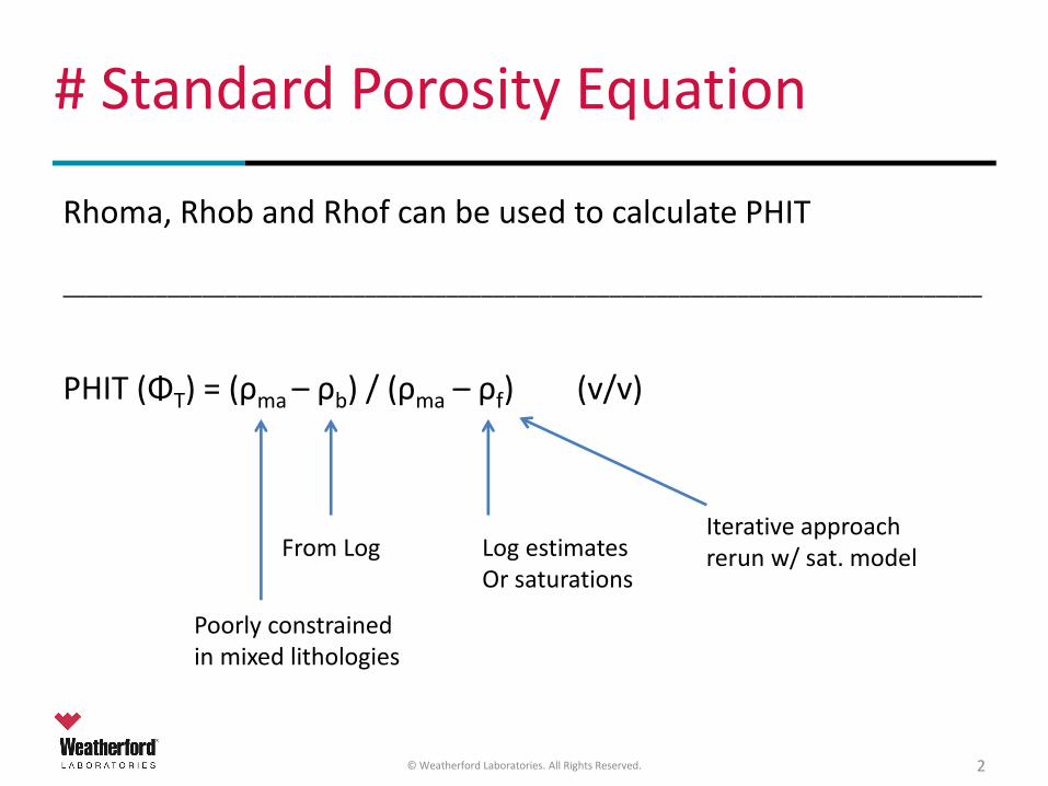
Rhoma, Rhob and Rhof can be used to calculate PHIT

_______________________________________________________________________________

PHIT (ΦT) = (ρma – ρb) / (ρma – ρf) (v/v)

# Standard Porosity Equation

Log estimates Or saturations

From Log

Poorly constrained in mixed lithologies

Iterative approach rerun w/ sat. model


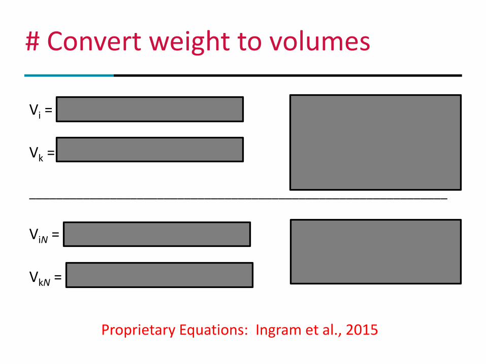
Vi = Mi(1 – Wk) x (ρma/ρmi) (v/v)

Vk = Wk x (ρma/ρk) (v/v)

______________________________________________________________

ViN = Vi / 𝑉𝑖𝑛𝑖 + Vk (v/v)

VkN = Vk / 𝑉𝑖𝑛𝑖 + Vk (v/v)

Vi = volume mineral (vol.%) Vk = volume kerogen (vol.%) Mi = mineral component (wt.%) ρma = rock matrix density (g/cc) ρmi = mineral density (g/cc) ρk = kerogen density (g/cc)

ViN = normalized mineral (vol.%) VkN = normalized kerogen (vol.%) ρma = cancels out here (g/cc)

# Convert weight to volumes

Proprietary Equations: Ingram et al., 2015


Bound fluids can be estimated given clay typing and volumes

_______________________________________________________________________________

Φclay = (ρclay-dry – ρclay-wet) / (ρclay-dry – ρf)

CBW = (Vclay1 x Φclay1) + (Vclay2 x Φclay2) + ….

PHIE (Φeff) = ΦT – CBW (v/v)

Φclay = bound water affinity (ratio) ρclay-dry = dry clay density (g/cc) ρclay-wet = dry clay density (g/cc) ρf = fluid density - brine 1.05 (g/cc) Vclay1 = volume clay (v/v) Φeff = effective porosity (v/v) ΦT = total porosity (v/v) CBW = clay bound water (v/v)

# Optional: CBW and PHIE est.

Sondergeld et al. 2012: SPE Paper

Material balance sum to 1.00

Multiple Volume by density

Organic Matrix = solid-phase kerogen and/or bitumen

Organic Matrix (K)ma & HM impart ΔRhoma if v/v is sufficient

Once solid-phase Rhoma is determined solve for PHIT


# Rhoma geochemistry derived

Vca

Pore Volume

Vqrtz

ρsand = 2.65 G/CC ρlime = 2.71 G/CC

VCL

0.15 0.4 0.4

Solid

-ph

ase Rh

om

a

0.05

Organic Matrix


Sum of mineral components and kerogen defines solid matrix

________________________________________________________________________________

ρma = 𝑉𝑖𝑁𝑛𝑖 x ρmi + VkN x ρk

ρma = solid-phase matrix density (g/cc) ρmi = mineral density (g/cc) ViN = normalized mineral (vol.%) VkN = normalized kerogen (vol.%) ρk = kerogen density (g/cc)

# Rhoma from geochemistry



• All mineral components and kerogen are closed around PHIT

___________________________________________________________________________________

• ViN(1 – ΦT) and VkN(1 – ΦT)

• If CBW > ΦT Then CBW = ΦT

ViN = normalized mineral (vol.%) VkN = normalized kerogen(vol.%) CBW = clay bound water (v/v) ΦT = total porosity (v/v)

# Close volumes around PHIT



Model Inputs

I. XRF Major Elements

II. DECT Rhob

III. Optional - logs

Calibrated Model

• XRD & XRF

• TOC & Pyrolysis

• Rock Properties (SRP)

Multimineral Model

Post-slabbed Core!

Proprietary Image






Outline

1. Start with lab TOC/Pyrolysis and XRD and/or XRF

2. Covert above to volumes using multimineral equations

3. Depth shift lab / core plug data as needed with SGR

4. Match above to log mineral model and kerogen curve

5. Adjust to match RHOMAA to RHOMAA from 1. (above)

6. Run log multimineral model and adjust to PHIT as needed

7. Optional – match clay minerals to CBW estimates

8. Select saturation model, plot core SW re-run MultiMin

9. Note – oil vs. water-wet zones much more involved SCAL


Core-Log Calibration Workflow


Workflow to maximize value

Core Acquisition Pre-slab non-destructive core analyses (DECT, SGR)

Yes

No

Visual description Yes

No

Pick Core Plugs

CT Mineral Model

Pick Core Plugs

Yes No

Sections / Plugs for Saturations

Slab Core

ASAP

XRF Multimineral Model

Yes No

Additional Core Plugs

TOC/Pyrolysis / XRD Re-calibrate Model

Fully Calibrate Petrophysical logs

Yes

No

1

2

3

1 = Fair 2 = Better 3 = Best


• It is critical calibrating petrophysical models, i.e. Vclay, PHIT

• Rock properties, plug location may bias reservoir assessment

Why is selecting plugs important?

Log Curve (x) Log Curve (x)

Lab

Dat

a (y

)

Lab

Dat

a (y

) Y = mx + b Y = mx + b

Statistical plugs Selected plugs

Skewed Representative R^2 << R^2

Log Calibration Questions

• What is the value of non-destructive core analyses?

• How can they help with core evaluation workflows?

• How is rock geochemistry properly compared to logs?

• What techniques best calibrate petrophysical models?

• How can such data be applied to formation evaluation?

30 © Weatherford Laboratories. All Rights Reserved.




4. Calibrating models with lab data core plug selection


END PRESENTATION


2.0

2.1

2.2

2.3

2.4

2.5

2.6

2.7

2.8

2.9

3.0

2.0 2.1 2.2 2.3 2.4 2.5 2.6 2.7 2.8 2.9 3.0

Dry

Gra

in D

en

sity

XRD Matrix Density

Lab validation examples of Rhoma


2

2.1

2.2

2.3

2.4

2.5

2.6

2.7

2.8

2.9

3

2 2.1 2.2 2.3 2.4 2.5 2.6 2.7 2.8 2.9 3

Dry

Gra

in D

ensi

ty

XRD Matrix Density

2

2.1

2.2

2.3

2.4

2.5

2.6

2.7

2.8

2.9

3

2 2.1 2.2 2.3 2.4 2.5 2.6 2.7 2.8 2.9 3

Dry

Gra

in D

ensi

ty

XRD Matrix Density

Lab validation examples of Rhoma

Multimineral Modeling - PTTC Rockiespttc.mines.edu/MM_Slides.pdf · 2015-07-07 · Multimineral...

Documents

Transcript of Multimineral Modeling - PTTC Rockiespttc.mines.edu/MM_Slides.pdf · 2015-07-07 · Multimineral...