Multigrid algorithms for inverse problems for the heat equation · 2012-06-08 · Inverse problems,...

MULTIGRID ALGORITHMS FOR INVERSE PROBLEMS WITH LINEARPARABOLIC PDE CONSTRAINTS ∗

SANTI S. ADAVANI † AND GEORGE BIROS‡

Abstract. We present a multigrid algorithm for the solution of distributed parameter inverse problems con-strained by variable-coefficient linear parabolic partial differential equations. We consider problems in which theinversion variable is a function of space only; for stability we use an L2 Tikhonov regularization. The main featureof our algorithm is that its convergence rate is mesh-independent—even in the case of no regularization. This featuremakes the method algorithmically robust to the value of the regularization parameter, and thus, useful for the casesin which we seek a high-fidelity reconstruction.

The problem is formulated as a PDE-constrained optimization. We use a reduced space approach. We eliminatethe state and adjoint variables and we iterate in the inversion parameter space using Conjugate Gradients. Weprecondition with a V-cycle multigrid scheme. The multigrid smoother is a two-step stationary iterative solver thatinexactly inverts an approximate Hessian by iterating exclusively in the high-frequency subspace (using a high-pass filter). We analyze the performance of the scheme for the constant coefficient case with full observations;we analytically calculate the spectrum of the reduced Hessian and the smoothing factor for the multigrid scheme.The forward and adjoint problems are discretized using a backward-Euler finite-difference scheme. The overallcomplexity of our inversion algorithm isO(NtN + N log2 N), where N is number of grid points in space and Nt

is the number of time steps.We provide numerical experiments that demonstrate the effectiveness of the method for different diffusion co-

efficients and values of the regularization parameter. We also provide heuristics, and conduct numerical experi-ments for the case with variable coefficients, and partial observations. We observe the same complexity as in theconstant-coefficient case. Finally, to avoid exact forward and adjoint solves far from the minimum, we combine thereduced-space algorithm with a full-space method.

Key words. Inverse problems, heat equation, reaction-diffusion equations, multigrid, regularization.

AMS subject classifications.

1. Introduction. In this paper we present multigrid algorithms for inverse problemsconstrained by parabolic partial differential equations (PDEs). As a model problem we con-sider the one-dimensional heat equation. The inversion parameter is a heat source, which wetry to reconstruct given full or partial observations of the temperature. Our method is designedfor problems in which the temporal variation of the heat source is known, but the spatial varia-tion is not. Our model is motivated by inverse medium and data assimilation problems that areconstrained by reaction-convection-diffusion equations. We use an an infinite-dimensionalPDE-constrained optimization formulation [5]. Although we consider only the 1D case, ouralgorithmic choices are designed for large-scale three-dimensional problems.

More precisely, we seek to reconstruct an unknown function u(x) by solving the follow-ing minimization problem:

miny,uJ (y, u) :=

12

∫Ω

∫T

(y(x)− y(x)∗)2 d Ωd t +β

2

∫Ω

u(x)2 d Ω,

subject to:

∂y(x)∂t

− ν∆y(x) = a(x, t)y(x) + b(x, t)u(x) in D, y = 0 on ∂Ω, y(x, 0) = 0 in Ω,

∗This work was supported by the U.S. Department of Energy under grant DE-FG02-04ER25646, and the U.S.National Science Foundation grants CCF-0427985, CNS-0540372, IIS-0431070, and DMS-0612578.

†Department of Mechanical Engineering and Applied Mechanics, University of Pennsylvania, Philadelphia, PA19104, USA ([email protected])

‡Departments of Mechanical Engineering and Applied Mechanics, Bioengineering, and Computer and Informa-tion Science, University of Pennsylvania, Philadelphia, PA 19104, USA ([email protected])

1

2 S. S. ADAVANI AND G. BIROS

where D is defined as Ω × (0, T ]. Here, y is the state variable, u is the inversion variable,ν > 0 is the diffusion coefficient, and β ≥ 0 is the regularization parameter. The objectiveis to reconstruct u by minimizing the misfit between the observed state y∗ and the predictedstate y. We assume that both a(x, t) and b(x, t) are known, smooth, and bounded functions.1

By forming a Lagrangian, introducing the adjoint variables λ, and by requiring station-arity with respect to the state, inversion, and adjoint variables, we arrive at the the first-orderoptimality conditions:State

∂y

∂t− ν∆y − ay − bu(x) = 0 in D, y = 0 on ∂Ω, y(x, 0) = 0 in Ω.

Adjoint

−∂λ

∂t− ν∆λ− aλ + (y − y∗) = 0 in D, λ = 0 on ∂Ω, λ(x, T ) = 0 in Ω.

Inversion

βu−∫

T

bλ d t = 0 in Ω.

The above system of equations is also known as the Karush-Kuhn-Tucker optimality systemor the “KKT” system. The corresponding linear operator can be written as I 0 − ∂

∂t − ν∆− a

0 βI −∫ T

0b

∂∂t − ν∆− a −b 0

=

Q 0 JT

0 βI CT

J C 0

. (1.1)

The KKT operator corresponds to a symmetric saddle point problem. For an excellent reviewon linear solvers for such problems, we refer the reader to [6]. In this paper we will considertwo methods, the so-called “full space” and “reduced space” [15]. In full space methods onesolves directly (1.1), for example, using a Krylov iterative method. In reduced space methodsone solves for u by an iterative solver on the the Schur complement of u. To derive the Schurcomplement, we first eliminate y and λ using the state and adjoint equations respectively, andthen we substitute λ in the inversion equation. In this way we obtain

Hu = g. (1.2)

The “reduced Hessian” H (or just “Hessian”) is defined by H = CT J−T QJ−1C +βI .Since Q is positive semi-definite, H is a symmetric and strictly positive definite operator. Thereduced gradient g is defined by g = −CT J−T Qy∗. We focus our attention to the designof efficient solvers for reduced space formulations. For completeness we include an examplethat shows how we can combine full and reduced space approaches.

Related work. Reduced space methods are quite popular because one can iterate on theadjoint and state equation in sequence, they require less storage, and the Conjugate Gradientsmethod (CG) can be used to invert H . The KKT matrix (1.1), is indefinite, ill-conditioned,and its size is more than twice as large as that of the forward problem. Most implementa-tions avoid using H and instead use some approximation, for example, quasi-Newton. Suchapproaches however, are not algorithmically scalable [1]. If H is to be used, direct solversare not a viable option since the reduced Hessian is a non-local and thus, dense operator. The

1In the following we suppress the notation for the explicit dependence on x and t.

MULTIGRID FOR INVERSE PROBLEMS WITH PARABOLIC PDES 3

Preconditioned Conjugate Gradients (PCG) algorithm requires matrix-vector product (here-inafter, “matvec”) operations only, and thus, can be used to solve (1.2).

If we fix the regularization parameter β to a positive value we can show that H is a com-pact perturbation of the identity and thus, has a bounded (mesh-independent) condition num-ber: it scales as O(1/β). Using CG to solve a linear system involving H requires O(1/

√β)

iterations. Therefore, the overall scheme does not scale with vanishing β. We claim that inmesh refinement studies and scalability analyses for inverse problem solvers, having a fixedvalue of β can lead to wrong conclusions.

There are two reasons that drive the need to solve problems in refined meshes. The firstreason is the need to resolve the forward and adjoint equations. In that case one can use amixed discretization in which u is discretized in a coarser grid, or one can use a large value forβ. In the second case, which is pertinent to scalability of the inverse problem solver, we havehigh-quality observations2 that allow for a high-resolution reconstruction of u. This impliesthat β cannot be fixed as we refine the mesh because we will not be able to recover the soughtfrequencies. Obtaining a mesh-independent scheme for vanishing β, to our knowledge, hasnot been addressed.

Returning to the reduced Hessian, we observe that the deterioration of the conditionnumber with decreasing β suggests the need for a preconditioning scheme. We cannot usestandard preconditioning techniques like incomplete factorizations or Jacobi relaxations, asthese methods need an assembled matrix [4]. In [7] a two-step stationary iterative methodthat does not need an assembled matrix was used to precondition the reduced Hessian. (Thetwo-step method will be the smoother in our scheme.)

Another alternative is to use multigrid methods. These methods have been developedmainly for linear systems arising from the discretization of elliptic and parabolic PDEs. Thebasic idea of multigrid is to accelerate the iterative solution of a PDE by computing correc-tions on a coarser grid and then interpolating them back to the original grid. The three impor-tant steps of multigrid scheme are pre-smoothing, coarse-grid correction and post-smoothing.Smoothing is equivalent to taking a few iterations of an iterative method (“smoother”) thatshould selectively remove the high-frequency error components faster than low-frequencycomponents. Besides the pioneering work of [12] for differential operators, and of [19] forsecond-kind Fredholm integral operators, there exists significant work on multigrid methodsfor optimal control problems. For example see the work of [2] and [15] for a general discus-sion, and [9] and [10] for distributed control problems constrained by parabolic PDEs. Analternative to multigrid is domain decomposition; a promising work for problems similar toours can be found in [21]. There the author proposes a space-time Schur domain decomposi-tion preconditioner for the KKT system. A nice feature of that method is that it can be readilyparallelized in time. The context however, is optimal control and not inverse problems: thevalue of the regularization parameter is quite large.

In our case, the unregularized reduced Hessian is a Fredholm operator of the first kind.There has been little work on multigrid algorithms for such problems. In [20] multilevel anddomain decomposition preconditioners were proposed for integral equations of first-kind.Multigrid solvers for Tikhonov-regularized ill-posed problems were discussed in [27] and[26]. Such problems were further analyzed in [24] and [25]. A multigrid preconditionerbased on that work was also used in [1] to solve problems with million of inversion param-eters. All these methods however, require a relatively small but non-vanishing value of theregularization parameter. As we will discuss later in the paper, the methods described in [1]and [10] do not scale well in the case of a mesh-dependent regularization parameter.

2If the data is not in the range of the inversion operator, e.g., due to noise, vanishing data will result in blow upfor u.


Contributions. Our main contribution is to derive a method for which we obtain a mesh-independent and β-independent convergence rate—including the case of β = 0. We designspecial smoothers that are used to built multigrid schemes for (1.2).

There are several challenges in designing multigrid schemes for the reduced space. Aswe mentioned, we have to design a matrix-free smoother with no access to diagonal or off-diagonal terms of the Hessian operator. The reduced Hessian (with β = 0) is a compactoperator. Its dominant eigenvalues correspond to low-frequency components and for suchoperators standard smoothers fail. Finally, every matrix-vector multiplication with the re-duced Hessian is equivalent to a forward and an adjoint solve; hence, it is important to designalgorithms that require a minimum number of matvecs in the fine grid.

We first propose a multigrid solver that uses a CG smoother combined with an approxi-mate filtering operator that restricts the CG iterations in the high-frequency Krylov subspace.We show numerical results that indicate good behavior. The method is easy to implement,but difficult to analyze. For this reason we propose a second smoother that is more expensivebut for which we can provide complexity estimates.

The main components of the proposed algorithm are: (1) a reduced Hessian that is acomposition of spectral filtering with an approximate Hessian operator based on inexactforward and adjoint solves; and (2) a smoothing scheme that uses a stationary second-ordermethod targeted in the high-frequency components of u. It is crucial that the effectivenessof the smoother in the high-frequency regime is mesh independent; our method fulfills thisrequirement. The multigrid scheme (a V-cycle) can be used as solver or as a preconditionerfor a Krylov iterative method.

The forward and adjoint problem are discretized using a backward-Euler scheme in time,and a standard three-point Laplacian (Dirichlet BCs) in space. We conduct numerical ex-periments to test (1) the effects of semi-coarsening (only space coarsening) and standard-coarsening; (2) different smoothing techniques; and (3) the effects of using non-Galerkincoarse-grid operators. We analyze and experimentally measure convergence factors. Also,we present results for the more general case in which multigrid is used as a preconditionerand not as a solver. In addition, we test the algorithm for the case of variable coefficients(resembling reaction-diffusion equations that admit traveling wave solutions) and partial ob-servations. Finally, we include a discussion on full-space methods and we propose a multigridscheme for (1.1) along with numerical results that illustrate its performance.

1.1. Organization of the paper. In Section 2 we derive the spectral properties of theanalytic and discretized reduced Hessian for the case of constant coefficients. In Section3 we discuss multigrid and we give details on the coarse-grid operator. In Section 3.2 wediscuss standard smoothers and present construction of novel smoothers based on the idea ofsubspace decomposition; in Section 4, we present appropriate preconditioners so that PCGcan be used as a smoother. Numerical results on this approach are presented in Section 4.1.In Section 5, we present our main contribution, a multigrid variant which based on exactsubspace projections, and we present results for both the constant and variable coefficientcase. Finally, in Section 6 we discuss full space methods.

2. Spectral properties of the reduced Hessian. We start by calculating the spectrumof the reduced Hessian. We show that in its general form, the source inversion is an ill-posed problem with algebraically decaying eigenvalues. Let K be the Green’s operator forthe forward problem, so that K maps functions from the inversion variable space to the statevariable space. Using K, we can eliminate the constraint and obtain an unconstrained varia-


tional problem for u:

min J (u) =12

∫Ω

∫T

(Ku− y∗)2 d Ωd t +β

2

∫Ω

u2 d Ω. (2.1)

Taking variations of (2.1) with respect to u we get an Euler-Lagrange equation for u:

∂J∂u

u =∫

Ω

∫T

KT (Ku− y∗)u d Ωd t + β

∫Ω

uu d Ω = 0,∀u, (2.2)

where KT is the adjoint of K. Then the strong form of the optimality conditions is given by(KT K + βI

)u = KT y∗ or Hu = KT y∗, (2.3)

where H is the reduced Hessian. If a = 0 then K (for homogeneous Dirichlet boundaryconditions) is given by

y =∫

Ω

∫ t

0

k(x− y, t− τ)b(x, t)u(x) d yd τ

= 2∞∑

k=1

∫Ω

∫ t

0

e−k2π2(t−τ)Sk(x)Sk(y)b(x, t)u(x) d yd τ, (2.4)

where Sk(x) = sin(kπx). If we assume that b = 1(t), expand u(x) =∑∞

j=1 ujSj(x), anduse orthogonality we get

y =∞∑

k=0

Sk(x)yk(t), with yk(t) =∫ t

0

e−k2π2(t−τ)1(τ)uk dτ. (2.5)

The adjoint operator KT is given by

λ(x, T − t) = KT z =∫

Ω

∫ t

0

k(x− y, t− τ) z(y, T − τ) d yd τ. (2.6)

Using (2.5) and (2.6) in (2.3), and setting β = 0, the eigenvalues (σk) and eigenvectors (vk)of the reduced Hessian (H = KT K) are given by

σk =2k2π2T + 4e−k2π2T − 2e−2k2π2T − 3

2k6π6and vk = Sk. (2.7)

If we discretize in space using the three-point Laplacian approximation, the correspond-ing eigenvalues and eigenvectors of the reduced Hessian (Hh) are given by

σk =2λkT + 4e−λkT − 2e−2λkT − 3

2λ3k

and vk = Shk , (2.8)

where λk = 4νN2 sin2( kπ2N ) is the kth eigenvalue of the discrete Laplacian and ν is the diffu-

sion coefficient. The discrete sine function is represented by Shk with N being discretization

size. If we use a backward Euler scheme for time the eigenvalues of the discrete reducedHessian (Hh) are given by

σδk = δ3

Nt∑j=1

Nt−j∑l=0

∑l+j−1r=0

1(1+λkδ)r

(1 + λkδ)l+1, (2.9)


100 101 102 103 10410−20

10−15

10−10

10−5

100

eigenvector number

eige

nval

ue (σ

)

Spectrum of H

β = σmin

β = 256σmin

β = 4096σmin

100 101 102 103 10410−15

10−10

10−5

100

eigenvector number

eige

nval

ue (σ

)

spectrum of H for different ν

ν = 1.0ν = 0.01ν = 0.0001

FIG. 2.1. Effect of regularization on the spectrum of the reduced Hessian. Here we report the Spectrumof eigenvalues (σ) of the reduced Hessian H for ν = 1.0 and T = 1. Three cases of regularization parameterβ = σmin, 256σmin, 4096σmin are plotted. The right plot shows the spectrum of H for three different diffusioncoefficients ν = 1, 0.01, 0.0001.

TABLE 2.1Eigenvalues, eigenvectors of Laplacian and reduced Hessian. The kth eigenvalue and eigenvector of the

operator are represented by σk and vk respectively. The diffusion coefficient and total time interval are ν and Trespectively. Here Sk = sin(kπx). Discrete operators and functions are denoted with a superscript h.

Operator σk vk

−ν∆ λk = νk2π2 Sk

−ν∆h λhk = 4νN2 sin( kπ

2N ) Shk

H σk = 2λkT+4e−λkT−2e−2λkT−32λ3

kSk

Hh σk = 2λhkT+4e−λh

k T−2e−2λhk T−3

2(λhk)3

Shk

Hh,δ σδk = δ3

∑Nt

j=1

∑Nt−jl=0

Pl+j−1r=0

1(1+λkδ)r

(1+λkδ)l+1 Shk

where Nt is the number of time steps and δ the time step.From (2.7) and (2.8) it is evident that k → ∞ ⇒ σk → 0. Furthermore σmax ≈ T

(λk)2 ,for a large-enough time-horizon T . If β 6= 0 then σmin = β and the condition number ofthe reduced Hessian is given by κ = σmax+β

β and it is bounded. For small β, however, thereduced Hessian is a highly ill-conditioned operator (see Figure 2.1).

TABLE 2.2CG mesh-dependence. Here we report the performance of CG as a function of the mesh size and the value

of the regularization parameter. The number of CG iterations does not change with an increase in the problem sizeNs; β is the regularization parameter and in parentheses the number of recovered frequencies; iters corresponds tonumber of CG iterations for a relative residual reduction ‖r‖/‖r0‖ ≤ 10−12; and maximum number of iterationsis 2Ns. Two cases of regularization parameter are considered: β = σ20 and β = σ100. Additional parametersused in this numerical experiment are ν = 1, T = 1. One observes that the number of CG iterations are mesh-independent only in the case of constant β.

Ns β (σ > β) iters512 6e-08 (19) 1e-10 (99) 69 7251024 6e-08 (19) 1e-10 (99) 70 7812048 6e-08 (19) 1e-10 (99) 68 7634096 6e-08 (19) 1e-10 (99) 71 713


The number of CG iterations required for convergence is proportional to the square rootof the condition number of the underlying operator. Therefore, for mesh-independent condi-tion number, we obtain a mesh-independent number of iterations. It may be the case however,that the data fidelity allows quite small regularization parameter.

In Table 2.2 we report results from a numerical experiment in which we study the numberof CG iterations for two cases of the regularization parameter. One can observe that forconstant β the the number of iterations is mesh-independent. This is not the case when βis related to the mesh size. The goal of the present work is to use multigrid ideas to addressproblem of β-independence number of CG iterations, at least for the source inversion problemfor the heat equation.

3. Reduced space multigrid. In this section we summarize the algorithmic issues re-lated to multigrid for the reduced Hessian. Here, and in the rest of the paper, we use thesuperscript h to denote the fine discretization level, and 2h the coarse level—in the case ofa two-grid scheme. For example, we denote the discrete reduced Hessian at resolution h byHh. The key steps of a multigrid algorithm for Hhuh = gh are given in Algorithm 1. The re-

Algorithm 1 Multigrid (MG)1: Pre-smoothing: Smoother iterations on Hhuh = gh

2: Restriction:rh = gh −Hhuh and r2h = I2hh rh

3: Coarse-grid correction: Solve H2he2h = r2h

4: Prolongation: eh = Ih2he2h

5: Update: uh ← uh + eh

6: Post-smoothing Smoother iterations on Hhuh = gh

striction (I2hh ), prolongation (Ih

2h) and coarse grid (H2h) operators are important componentsthat determine the performance of the algorithm. In Table 3.1 we summarize the spectra ofseveral restriction and prolongation based operators. Key in a multigrid scheme is to that each

TABLE 3.1Spectral properties of the restriction and prolongation operators. Let sk = sin2( kπx

2), ck = cos2( kπx

2)

and Sk = sin(kπx) for 1 ≤ k ≤ N−1. I2hh : Ωh → Ω2h, Ih

2h: Ω2h → Ωh and I− Ih2hI2h

h : V h → W 2h whereV h is the fine space and W 2h is the space containing high frequency components. Sh

k , S2hk are the eigenfunctions

of the discrete Laplacian and the reduced Hessian in Ωh and Ω2h respectively. 1 ≤ k ≤ N2

for all the rows in theTable.

Operator Input function Output functionI2hh Sh

k ckS2hk

I2hh Sh

N−k −skS2hk

Ih2h S2h

k ckShk − skSh

N−k

I− Ih2hI2h

h Shk (1− c2

k)Shk + ckskSh

N−k

I− Ih2hI2h

h ShN−k (1− s2

k)ShN−k + ckskSh

k

grid level the majority of the work is in removing errors associated with high-frequencies (atthe specific grid level). In addition as we move into the grid hierarchy, errors should not bereintroduced or amplified. The problems we are discussing here are pretty regular so pro-longation and restriction do not present particular challenges. Below we first discuss thecoarse-grid operator representation and then we discuss smoothing techniques.

3.1. Coarse-grid operator. There are two main ways to define the coarse-grid operator,given a grid-hierarchy, the Galerkin and the direct discretization. Using a variational principle


and provided that I2hh = cIh

2hT , the “Galerkin” coarse-grid operator operator is defined by

H2hG = I2h

h HhIh2h,

where H2hG and Hh are the Galerkin coarse-grid operator and fine grid operators respectively

[13]. Another way of defining the coarse-grid operator is by discretizing directly the forwardand adjoint problems in the coarse grid:

H2h = (CT J−T )2hQ(J−1C)2h.

In the classical multigrid theory for the Laplacian operator on regular grids with constant-coefficients there is no difference between the two coarse-grid operators. In the case of re-duced Hessian, however, they are quite different—especially in the high-frequency region ofthe coarse space (Figure 3.1). The difference in the spectra can be explained from the scalingof the eigenvalues of Hh due to the eigenstructure of the standard restriction and prolonga-tion operators (Table 3.1). Therefore, error components in certain intermediate eigenvectordirections of the fine grid spectrum cannot be recovered if we use H2h. So it is preferable touse the Galerkin coarse-grid operator for robustness and easily provable convergence. On theother hand every Galerkin coarse-grid matvec requires a fine-grid reduced Hessian matvecwhich makes it computationally expensive. Therefore, we avoid using H2h

G and use H2h.

100

101

102

10−8

10−6

10−4

10−2

eigenvector

eige

nval

ue

Ih2h Hh I

2hh vs H2h

Ih2h Hh I

2hh

H2h

FIG. 3.1. Spectrum of the coarse-grid reduced Hessian. Here we depict the difference between the GalerkinI2hh Hh Ih

2hand the direct discretization of the reduced Hessian operators. We observe that H2h does not satisfythe Galerkin condition, and thus, inverting it will not eliminate the low frequency components of the error. Due tothis fact we use multigrid as a CG preconditioner.

3.2. Smoothers. Classical smoothing schemes for the elliptic PDEs include iterativemethods like Jacobi, Gauss-Seidel and CG. A common characteristic of these methods is thatthey remove error components corresponding to large eigenvalues faster than error compo-nents corresponding to small eigenvalues.3 This property makes these methods favorable forelliptic operators that have large eigenvalues for high frequency eigenvectors. In our case,the (unregularized) reduced Hessian is a compact operator and behaves quite differently. Asshown in Figure 2.1, large eigenvalues of the reduced Hessian are associated with smootheigenfunctions and small eigenvalues are associated with rough or oscillatory eigenfunctions.

3CG works on both ends of the spectrum, but this is not so important in our context.


Therefore, the above smoothing methods act as roughers. In addition, we do not have di-rect access to the entries of the reduced Hessian matrix so there is no cheap way to applysmoothers like Jacobi or Gauss-Seidel.

We discuss in a greater detail why CG cannot be used as a smoother. Using (2.7) wewill show that CG cannot be used as a smoother for this problem as it acts on the high energy(large eigenvalues) smooth components and acts as rougher instead. We neglect the expo-nential terms as they go to zero very fast. Let β = 0 and T = π4, then the kth eigenvalueof the reduced Hessian is σk = 1

k4 . At the ith iteration, CG constructs an (i − 1)th degreepolynomial to minimize ‖e(i)‖H . Therefore the error at the ith iteration can be expressed ase(i) = Pi(σ)e(0), where Pi(σ) is the (i− 1)th degree polynomial, e(0) is the initial error ande(i) is the error at ith iteration. Pi(σ) is given by Chebyshev polynomials, where the Cheby-shev polynomial Ti(ω) of degree i is Ti(ω) = 1

2

[(ω +

√ω2 − 1)i + (ω −

√ω2 − 1)i

], [28].

The polynomial Pi(σ) is given by

Pi(σ) =Ti

(σmax+σmin−2σ

σmax−σmin

)Ti

(σmax+σmin

σmax−σmin

) .

We have already seen that the reduced Hessian is a compact operator. Thus, neglectingσmin (σmin σmax) gives Pi(σk) = Ti

(1− 2

k4

). Without loss of generality, we can

assume that the initial guess has error components in all the eigenvector directions. Noticethat Pi(σk) is the amount of attenuation of the kth eigenvector at the ith CG iteration. Forhigh-frequency error components Pi(σk) ≈ Ti(1) = 1; for small k ≈ Pi(σk) = 0.5. Thus,amplitude reduction of low frequency error components is greater than that of high frequencyerror components: CG can not be used as a smoother in the present problem.

This motivates a modification of the Hessian operator so that the low-frequency spec-trum is screened out from CG. In this regard, we discuss construction of smoothers basedon the idea of decomposing the finite-dimensional space into relatively high-frequency andlow-frequency subspaces given in [27], [26]. This idea was further studied in [24], [25]. Sim-ilar ideas of using the subspace decomposition are also used in the construction of efficientpreconditioners in [18].

Our preconditioners will be based on a fine-coarse grid decomposition of the reducedHessian. The “coarse” space V 2h is embedded into the “fine” space V h. By Ph : V h → V 2h

we denote the L2-orthogonal projection, and by I − Ph : V h → W 2h the projection to highfrequency functions W 2h. We decompose v ∈ V h into a smooth component vs ∈ V 2h, andan oscillatory component wo ∈W 2h. Then Hhv = Hhvs+Hhwo. If in addition, we assumethat Ph coincides with the eigenvectors of the reduced Hessian (as it is in the case of constantcoefficients) we can write Hh as

(I − Ph + Ph)Hh(I − Ph + Ph) = (I − Ph)Hh(I − Ph) + PhHhPh (3.1)

assuming that Ph is the exact orthogonal projection operator i.e.,

(I − Ph)HhPhu = PhHh(I − Ph)u = 0, ∀u ∈ V h. (3.2)

Therefore we can write Hhu = g as,

(I − Ph)Hh(I − Ph)u + PhHhPhu = (I − Ph)g + Phg. (3.3)

Hence PhHhvs = Phg, and

(I − Ph)Hhwo = (I − Ph)g. (3.4)


Since we are interested in removing the high-frequency error components while smoothingwe solve (3.4). However, since in general Ph will not correspond to the high-frequencyspectrum of the Hessian, we can use it as an approximate projection. An alternative approachis to use Chebyshev iterative methods and work on the spectrum of interest, provided wehave eigenvalue estimates [3]. In principle, this method is quite similar to our approach(it is used for an entirely different problem.) It uses a number of reduced Hessian matvecoperations and computes an exact decomposition. In the present case, we would like to avoidspectra calculations, if possible, as our main goal is to minimize the number of matrix-vectormultiplications with the reduced Hessian. (For our smoother in Section 5 we only need thespectra range, and not all the eigenvalues.) Instead we approximate I − Ph either by standardinterpolation-restriction operators or by using Fourier transforms.

Based on these decompositions we present a smoother that uses PCG for (3.4) andI2hh Ih

2has an approximation to Ph (Section 4). The advantage of this scheme is its straight-forward implementation. However, it is hard to analyze its convergence for reasons that wewill discuss in the following sections. We also present a second smoother in which we usea two-step stationary solver that acts exclusively on the high-frequency spectrum using exactfrequency truncations for Ph (Section 5).

4. PCG smoother and restriction-prolongation projection. We will consider twoschemes. In the first one we use a V-cycle multigrid as a solver. In the second one weuse multigrid as a preconditioner for CG. In both schemes we will use a few iterations ofPCG as a smoother (within multigrid). Our contribution here, is the design of appropriatepreconditioners for the PCG smoothing iterations. The preconditioner will be based on aninexact inversion of the (I − Ph)Hh. To that end we need to approximate Ph and Hh ap-proximations one for Ph and one for Hh; Ph will be approximated by I2h

h Ih2h since this

approach generalizes to arbitrary meshes and it is easy to implement. For Hh we will exploretwo approaches, one based on the regularization parameter (King preconditioner) and onebased on inexact solves of the forward and adjoint solves (Pointwise preconditioner).

KING PRECONDITIONER. This approach was proposed by King in [27] where multigridmethod for first kind of integral operator equations were developed. From Figure 2.1, wecan see that if the regularization parameter β is sufficiently large, it can approximate mostof the high frequency spectrum. Therefore, eigenvalues corresponding to the high-frequencyeigenvectors will be β so that β(I − Ph)I ≈ (I − Ph)Hh. Substituting this in the (3.4) weget a single-level preconditioner of the form β−1(I − Ph). In a additional approximationstep we substitute the orthogonal projection by standard interpolation-restriction operators.Therefore the single-level King preconditioner is given by β−1(I − Ih

2hI2hh ).

In Table 3.1, we summarize the spectral properties of the restriction operator I2hh , pro-

longation operators Ih2h, and the orthogonal decomposition operator I− Ih

2hI2hh .

POINTWISE PRECONDITIONER. The pointwise preconditioner is based on a pointwiseapproximation of the reduced Hessian, combined with the high-frequency filtering describedin the previous section. The approximate reduced Hessian Hh should approximate well thehigh-frequency of the true Hessian (for β = 0) and should be easy to compute. Here wepropose a simple waveform-Jacobi relaxation in time. If we discretize in space using thestandard three point stencil for the Laplacian on a uniform grid, and introduce a space-Jacobisplitting a matrix vector multiplication with the reduced Hessian (in the frequency domain)


is given by

∂y

∂t+

2ν

N2y − 2ν

N2cos

kπ

Ny = u, solve for y

∂λ

∂t+

2ν

N2λ− 2ν

N2cos

kπ

Nλ + y(T − t) = 0, solve for λ

v =∫

λ, v = Hu.

Here k is the wavenumber, and y, λ and u represent the magnitude of the kth eigenvector.The approximate waveform Jacobi relaxation is given by

∂yi

∂t+

2ν

N2yi −

2ν

N2cos

kπ

Nyi−1 = u, i = 1 . . .M

∂λi

∂t+

2ν

N2λi −

2ν

N2cos

kπ

Nλi−1 + yM (T − t) = 0, i = 1 . . .M

v =∫

λM , v = Hu.

The number of iterations M determines the quality of the preconditioner. So far we have onlydiscretized in space. We use a Backward-Euler scheme to discretize in time. The number oftime steps equals the number of discretization points in space. Next, we discuss numericalexperiments in which we compare the two preconditioners.

TABLE 4.1Performance of multigrid solver with PCG smoother. We report results for a V-cycle multigrid solver. The

King and pointwise preconditioners are used in PCG. Here Ns is the size of the problem, β is the regularizationparameter. The number of resolved frequencies (number of eigenvalues that are greater than β are reported inbrackets); K-PCG corresponds to the number of V(3, 3) cycles with King preconditioner and PF-PCG correspondsto the number of V(3, 3) cycles with pointwise preconditioner. Convergence factors, ρK and ρPF , are the av-erage of convergence factors over all the V-cycles till convergence. Stopping criterion for the multigrid solver is‖r‖/‖r0‖ ≤ 10−12. Two cases of regularization parameter are considered: Case 1: β = 10−3h2/ν and Case2:β = 10−2h2/ν. ’-’ means that the multigrid solver hasn’t converged within the 50 V-cycles. Numerical experi-ment are done for ν = 1, ν = 0.01 with T = 1. At the coarsest level Ns = 16.

ν = 1

Ns β (σ > β) K-PCG PF-PCG ρK ρPF

512 4e-09 (40) 4e-08 (22) 14 6 7 6 0.239 0.171 0.041 0.0221024 1e-09 (57) 1e-08 (32) - 7 8 6 0.493 0.174 0.076 0.0582048 2e-10 (81) 2e-09 (45) - 13 8 6 0.573 0.253 0.162 0.0534096 6e-11 (114) 6e-10 (64) - 12 9 6 0.704 0.206 0.150 0.104

ν = 0.01

Ns β (σ > β) K-PCG PF-PCG ρK ρPF

512 4e-07 (131) 4e-06 (72) 22 7 5 5 0.359 0.294 0.007 0.0041024 1e-07 (183) 1e-06 (102) 29 9 7 6 0.474 0.385 0.025 0.0142048 2e-08 (257) 2e-07 (144) - 13 8 6 - 0.164 0.074 0.0334096 6e-09 (363) 6e-08 (203) - 19 9 7 - 0.322 0.118 0.089

4.1. Numerical experiments for the PCG smoother. We report numerical experimentsin which we compare the the effectiveness of a V-cycle multigrid for (1.2). The V-cycleuses linear finite element based interpolation and restriction operators, and preconditioned


TABLE 4.2Performance of PCG as a solver with multigrid preconditioner with PCG as smoother in multigrid. N is the

size of the problem, none corresponds to number of PCG iterations without preconditioner. K-PCG correspondsto the PCG iterations with multigrid preconditioner V(3, 3), with King preconditioner in PCG smoother. PF-PCGcorresponds to the number of PCG iterations with multigrid preconditioner V(3, 3) with Pointwise preconditioner inPCG smoother. Values in the brackets represent equivalent number of matvecs done at finest level. Stopping criterionfor PCG is ‖r‖/‖r0‖ ≤ 10−12. Two cases of regularization parameter: Case 1 is β = 10−3h2 and Case 2 isβ = 10−2h2 are considered. Coarsest level is 16. Parameters used are ν = 1 and ν = 0.01 with T = 1.

ν = 1

N β(σ > β) none K-PCG PF-PCG512 3. 81e-09 (40) 3. 81e-08 (22) 167 81 9 (63) 4(28) 5 (35) 4(28)1024 9. 54e-10 (57) 9. 54e-09 (32) 267 117 14 (98) 5(35) 6 (42) 4(28)2048 2.38e-10 (81) 2.38e-09 (45) 516 192 22 (154) 8(56) 6 (42) 5(35)4096 5. 96e-11 (114) 5. 96e-10 (64) 1007 350 28 (196) 11(77) 6 (42) 5(35)

ν = 0.01

N β(σ > β) none K-PCG PF-PCG512 3. 81e-07 (131) 3. 81e-06 (72) 959 329 24 (168) 6(42) 4 (28) 4(28)1024 9. 54e-08 (183) 9. 54e-07 (102) 1780 642 41 (287) 7(49) 5 (35) 5(35)2048 2.38e-08 (257) 2.38e-07 (144) 3453 1201 99 (693) 9(63) 6 (42) 5(35)4096 5. 96e-09 (363) 5. 96e-08 (203) 7245 2522 498 (3486) 13(91) 7 (49) 6(42)

Conjugate Gradients as a smoother. Two cases of regularization parameter are considered4:β = 10−3h2

ν , 10−2h2

ν . We also study the effect of the diffusion coefficient. We considertwo cases of diffusion coefficient: ν = 1, 0.01 are considered in the spectral domain. In allthe numerical results given below, convergence factor is defined as the average of the ratioof the residuals resulting from two V-cycles. In all experiments H is constructed using 20waveform-Jacobi iterations for the adjoint and forward problems. In Table 4.1, results aregiven for multigrid solver. The PCG smoother with pointwise preconditioner converges inall the cases where as King preconditioner fails to converge in case of β = 10−3h2/ν. Thepointwise preconditioner is faster than the King preconditioner in case of β = 10−2h2/ν.Despite the fact that they have almost the same effect on the reduced Hessian at the finest levelthey behave differently at coarser levels. In Figure 4.1 the effect of these two preconditionerson the reduced Hessian is shown for coarser levels.

The pointwise preconditioner has the same effect on the reduced Hessian even at coarserlevels unlike King preconditioner. From Figure 4.1 for β = 10−3h2, KH has little or noclustering of eigenvalues near high frequency eigenvectors at level 8 whereas PFH has sig-nificant clustering. In case of β = 10−2h2, both KH and PFH have significant clusteringof eigenvalues near high frequency eigenvectors and PFH has more clustering than KHwhich makes PFH faster. Therefore, the effect of the preconditioner on the reduced Hessianat different levels in multigrid is important to predict the performance of the preconditionerin PCG.

Since we are not using an exact coarse-grid operator, we also test multigrid as a pre-conditioner within a PCG solver (Table 4.2). In both the cases, we can solve the problem

4The regularization parameter is chosen to trade off stability and fidelity to the data. In the present problem,the discretization error is of O(h2) and acts as a noise to the problem. In these synthetic experiments (in which wecommit several “inverse crimes”, [14]) we know the exact spectrum of the reduced Hessian, the level of noise, andour reconstructed solution is expected to be smooth. So the choice regularization is not an issue. In the general case,the choice of regularization is of paramount importance. But this is beyond the scope of this paper.


100 101 102 103 10410−5

100

105

eigenvector number

eige

nval

ue

Spectrum of KH, β = 10−3h2

level = 8level = 10fine level = 12

100 101 102 103 10410−5

100

105

eigenvector number

eige

nval

ue

Spectrum of PFH, β = 10−3h2


100 101 102 103 10410−5

100

105

eigenvector number

eige

nval

ue

Spectrum of KH, β = 10−2h2


100 101 102 103 10410−5

100

105

eigenvector number

eige

nval

ue

Spectrum of PFH, β = 10−2h2


FIG. 4.1. Comparison of the spectrum of the preconditioned reduced Hessian. We report the discretespectrum of the preconditioned reduced Hessian with King preconditioner (KH) and pointwise (PFH) preconditionerin spectral domain for the finest level and different coarser levels. The PFH preconditioner has similar clustering ofeigenvalues at high-frequency region at finer and coarser levels for different values of regularization parameter. KHdoes not show similar trend at finer and coarser level for different values of regularization parameter. This is thereason for the robust performance of PFH and failure of KH for smaller regularization parameters.

1 2 3 4 5 6 7 8 9 10 11 1210−15

10−10

10−5

100

number of V(3,3) cycles

rela

tive

resi

dual

r/r 0

β = 10−3h2

K−CGPF−CGCG

1 2 3 4 5 6 7 8 9 10 11 1210−15

10−10

10−5

100

number of V(3,3) cycles

rela

tive

resi

dual

r/r 0

β = 10−2h2

K−CGPF−CGCG

FIG. 4.2. V-cycle residual wrt regularization parameter. Relative residual vs V(3, 3) cycles with PCGsmoother for two cases of regularization parameter are shown. In this Figure, we compare the rate at which theresidual decreases for different preconditioners used in PCG smoother for two cases of regularization parameters.Case 1: β = 10−3h2 is shown on the left and Case 2: β = 10−2h2 is shown on the right where h = 1/4096.King’s preconditioner (K-CG) converges in Case 2 and fails to converge in Case 1. Pointwise (PF-CG) precondi-tioner converges in both the cases. CG fails as a smoother in both the cases.


in O(1) iterations as shown in the numerical results. This is equivalent to solving the for-ward and adjoint problems a constant number of times independent of the mesh size and theregularization parameter.

The King preconditioner has negligible computational cost when compared to the actualreduced Hessian matvec. In case of pointwise preconditioner there is an overhead associ-ated in computing H−1 every iteration. For a given residual reduction, it takes of constantnumber of CG iterations to invert Hh. Since the residual reduction is close to machine accu-racy, (Hh)−1 is a linear operator and creates no convergence problems in the smoother. Thecomputational cost of evaluating H−1, however, is much higher than the cost associated withapplying the King preconditioner. When the regularization parameter is large the pointwisepreconditioner is not necessary. Overall however, the latter is more robust. As seen from thenumerical results, pointwise preconditioner converges for different cases of regularization pa-rameters and diffusion coefficients unlike King preconditioner, which works only for largerregularization parameters. Therefore, pointwise preconditioner can be used in general thoughit has more computational overhead than the King preconditioner. Solving the forward andadjoint problems has a computational complexity 5 of O(N2

s ) using multigrid algorithms tosolve the linear algebraic system of equations at each time step in case of linear problems,where Ns is the number of grid points.

5. Two-step stationary scheme as smoother and FFT filtering. As discussed above,the King preconditioner fails in the case of smaller regularization parameters and the point-wise preconditioner, though robust, has an overhead of computing the inverse of the approx-imate reduced Hessian at every iteration. The combination of multigrid with PCG and thepointwise preconditioner performs well, at least for the simple model. Our target applicationultimately will involve variable coefficient problems and partial observations. In those caseswe expect a higher number of iterations. Although we can use multigrid as a solver it wouldbe preferable to combine it with an outer PCG acceleration. Due to the non-stationarity ofour scheme, however, this cannot be done.

As an alternative we propose to use an iterative two-step stationary scheme [16] (algo-rithm 2) as a smoother. Then, in the constant-coefficient case, one can derive exact smoothingfactors. As in classical multigrid theory [12, 19], the analysis becomes approximate in thecase of variable coefficients. One disadvantage of the two-step solver is that it requires esti-mates of extreme eigenvalues. To avoid computing eigenvalues we use a the spectral cutoffand analytic spectrum estimates. In this manner the smoother is forced to iterate on the high-frequency regime. In the following we present the algorithm in detail, analyze its convergencefactor, and conduct numerical experiments to test our hypothesis.

Algorithm 2 Standard two-step stationary iterative scheme (Solve AdT = din)1: σ1 = σmin(A) and σn = σmax(A)2: ρ = 1−σ1/σn

1+σ1/σn, α = 2

1+(1−ρ2)1/2 , ξ0 = 2σ1+σn

, ξ = 2ασ1+σn

,3: r = −din, d0 = 0, d1 = ξ0r4: for i = 1 . . . L do5: r = Ad1 − din

6: d = αd1 + (1− α)d0 − ξr7: d0 = d1, d1 = d8: end for

Since we are interested in removing the high-frequency error components while smooth-

5Nt = O(Ns)


ing, we iterate on (3.4) in the smoothing step. In (3.4) the projection operator I − Ph can bedefined as a filter which removes the eigenvector components corresponding to small wavenumbers. Let us denote the filtering operation by W = I − Ph. In the present problem,the eigenvectors are sines. Therefore, we can use discrete sine transforms to filter the low-frequency components of an input vector (algorithm 3).6

Algorithm 3 Projection using Sine Transform1: Let u be the input vector and let v = Wu2: uk = IDST(u) 1 < k < N − 1 transform into spectral domain3: uk = 0 1 < k < N−1

2 filtering in spectral domain4: v = DST(uk) transform back to spatial domain

5 10 15 20 25 30

10−20

10−15

10−10

eigenvector

eige

nval

ue

Spectral properties of WH

FIG. 5.1. Eigenvalues for the spectrally filtered re-duced Hessian. Here we report the magnitude of the eigen-values of the reduced Hessian. Here the W operator repre-sents an exact high-pass filter. During multigrid smoothing,the composite operator WH is inexactly inverted using atwo-step stationary iterative solver.

The problem that we solve during the smoothing iterations is

WHhu = Wg. (5.1)

Since the null space of W is non-trivial (5.1) is singular. However, it is proved that a positivesemi-definite system of the form (5.1) can be solved by preconditioned conjugate-gradientmethod (PCG) as long as the right-hand side is consistent [23]. The two-step iterative schemerequires that all the eigenvalues of the matrix (WHh) be positive (see section 5.2.3 in [4]).Let W = ZZT where Z = [vN+1

2, . . . , vN−1] in which vk correspond to the kth eigenvector

of Hh. The subspace spanned by the eigenvectors [v1, . . . , vN−12

] is invariant and does notinfluence the convergence rate of the two-step iterative solver.

We define one smoothing step as one iteration of the two-step scheme. In case of non-zero initial guess, the error el after l smoothing iterations is given by

el = ((α− 2αWH

σ1 + σn)(1− 2WH

σ1 + σn) + (1− α))le0, (5.2)

where e0 is the initial error and α is defined in Algorithm 2; σ1 and σn in (5.2) are definedlater. Let e0 = ΣN−1

k=1 mkvk where vk are the eigenvectors of H and mk are the correspondingerror magnitudes. Assuming that W results in an exact decomposition (3.2) eigenvalues ofWH are σ(WH) = 0, 0, . . . , σN+1/2, . . . , σN−1, where σk correspond to the kth eigen-value of the reduced Hessian H . Substitute e0 in (5.2) and take one smoothing iteration, weget e1

k = mkvk, ∀ 1 < k < N−12 , where e1

k is the error component in the kth eigenvector

6this is true only in the present case.


direction after one smoothing iteration. Similarly,

e1k = ((α− 2ασk

σ1 + σn)(1− 2σk

σ1 + σn) + (1− α))︸︷︷︸

µk

mkvk, ∀ N + 12

< k < N − 1.

Here µk is the amplification factor of the error component in the kth eigenvector direction.The eigenvalues σ1, . . . , σN−1/2 do not affect the iteration. The smoothing factor µ is givenby maxk(µk). To estimate µ we need estimates of σ1 and σn. For the constant coefficientcase we have computed these values analytically by (2.9): we fix the values of σ1 and σn tobe σN and σ(N+1)/2 respectively. Then, since σ1 ≤ σk ≤ σn we have µk < 1 ∀ N+1

2 < k <N − 1. Using the exact spectrum we can also show that the ratio σ1/σn = 1/4 and it is meshindependent (for β = 0). In the variable coefficient case we use a heuristic. We estimate σn

of the unregularized Hessian using a Krylov method on the reduced Hessian. Then, guided bythe constant coefficient case, we set σ1 = σn/4. For this ratio the smoothing factor µ is 0.288for ν = 1, 0.01. In two-level V(2,2) cycles if we use the Galerkin coarse-grid operator (H2h

G ),

TABLE 5.1Convergence for zero regularization parameter. Number of two-grid V(2,2)-cycles to get a relative residual

of 10−8, V1, V0.01 for ν = 1, 0.01 are given when β = 0. The size of the problem is 2level. The initial guessu0 = u∗ + Σksin(kπx), where u∗ is the exact solution. The theoretical smoothing factor is 0.288 and thenumerical is 0.29, and it is mesh independent.

level V1 V0.01

4 16 225 22 276 25 327 26 348 24 33

some low frequency error components are eliminated in the first V-cycle. In Figure 5.2 wecan see that relative residual drops suddenly in the first V-cycle and maintains a constant ratiothereafter. Whereas, the reduction in the error is constant which is expected. The sudden dropin the relative residual is because of the coarse-grid correction where the low-frequency errorcomponents are removed.

According to the spectrum of Hh low-frequency error components correspond to largeeigenvalues and since r = He, there is a sudden drop in the residual. After the first V-cycle,the reduction in the residual is less than the first V-cycle. We report the number of V-cyclesto get a relative residual of 10−8 in Table 5.1 for different mesh-sizes and two diffusioncoefficients ν = 1, 0.01. The number of V-cycles is mesh-independent.

5.1. Multigrid preconditioner. As we have mentioned, one difficulty in designing amultigrid scheme for the reduced Hessian operator is the choice of the coarse grid operator.If we use H2h instead H2h

G we cannot remove certain error components that belong to theintermediate frequency range (of the fine-grid). These error components are neither removedby the 2-step scheme nor by the coarse-grid correction. Therefore, we use multigrid as apreconditioner in PCG so that PCG removes the error components that are not removed bymultigrid.

We denote the multigrid preconditioner by M−1 (algorithm 4) and the smoothing oper-ator by S(A, f, u) where A, f , u are the matvec operator, the right hand side and the initialguess respectively. We denote inexact multigrid preconditioner by M−1 in which exact re-duced Hessian Hh is replaced by inexact reduced Hessian Hh in smoothing. Hh is obtained


5 10 15 20 2510

−15

10−10

10−5

100

V(2,2) cycles

||r||/

||r0||

relative residual

5 10 15 20 2510

−10

10−8

10−6

10−4

10−2

100

V(2,2) cycles

||e||

error

FIG. 5.2. Residual reduction in multigrid. Relative residual and error vs number of two-level V(2,2) cyclesfor ν = 1 and level six and using H2h

G as the coarse-grid operator.

by replacing exact forward and adjoint solves to do one reduced Hessian matvec by inexactforward and adjoint solves. In order to do this, we use a fixed number of Jacobi waveformrelaxation iterations [29]. The number of waveform relaxation steps have to be increasedin order to get a completely scalable algorithm because of the convergence properties of theJacobi waveform relaxation method.

Algorithm 4 Two-level exact multigrid Preconditioner (uh = M−1fh)

1: uh = S(WHh,Wfh, 0) pre-smoothing with Hh

2: rh = fh −Huh residual evaluation3: r2h = I2h

h rh restriction4: e2h = (H2h)−1r2h coarse-grid correction5: eh = Ih

2heh prolongation6: uh = uh + eh correction7: uh = S(WHh,Wfh, uh) post-smoothing with Hh

In the Jacobi waveform relaxation, we solve ordinary differential equations at every spa-tial grid point, thus removing the spatial-coupling that arises from the discretization of theLaplacian operator. This is different from the standard spatial weighted Jacobi scheme. The(high-frequency) convergence factors of weighted Jacobi method are mesh-independent—unlike the Jacobi waveform relaxation that gives rise to mesh-dependent convergence factor[29].7

5.2. Results and discussion. In this section, we present results for the constant andvariable coefficient case, as well as the case in which we have partial observations. We reportPCG iterations with multigrid preconditioners M−1 and M−1. We also show the sensitivityof number of Jacobi waveform relaxation steps on the number of PCG iterations. We presentnumerical results that interrogate the sensitivity of the scheme on the diffusion coefficient,the number of waveform relaxations, and the coarsening strategy (semi-coarsening or spaceonly vs standard space-time coarsening).

5.2.1. Constant coefficients case. Results for two cases of diffusion coefficients ν =1, 0.01 are given in Table 5.2. The convergence of PCG is mesh independent. We are re-porting results for both two-level and multiple V-cycle preconditioners. The cost of the pre-conditioner depends on the approximation of the reduced Hessian. Exact matvecs are more

7One could use standard time marching schemes in which exact inversions of the spatial operator can be replacedby an inexact solve, like weighted Jacobi.


expensive. For fixed number of waveform relaxations the quality of the approximate Hessiandeteriorates with increasing mesh size. The condition number of Hh is κ = O(N4) where Nis the size of the problem. Therefore, without a preconditioner number of CG iterations willbe O(N2). By using multigrid preconditioner number of CG iterations is mesh-independentO(1). Using a Backward-Euler time-stepping combined with an optimal spatial solver forthe forward and adjoint problems the amount of work done for each reduced Hessian matvecis O(NNt + N log2 N) where the first term comes from the forward and adjoint solve withNt time steps, and the second part comes from the multigrid sweeps (the square in the loga-rithm is related to the fast sine transforms). Therefore, the total amount of work done to solvethe system is brought down from O(N4) to O(N2). To solve the inverse problem we needto solve the forward problem a constant number of times independent of the regularizationparameter and the mesh size.

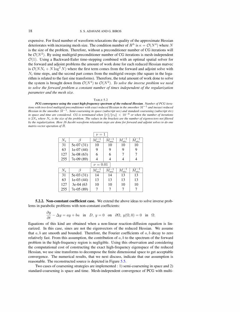
TABLE 5.2PCG convergence using the exact high-frequency spectrum of the reduced Hessian. Number of PCG itera-

tions with two-level multigrid preconditioner with exact reduced Hessian in the smoother M−1 and inexact reducedHessian in the smoother M−1. Semi-coarsening in space (subscript sec) and standard coarsening (subscript stc)in space and time are considered. CG is terminated when ‖r‖/‖r0‖ < 10−8 or when the number of iterationsis 2Ns where Ns is the size of the problem. The values in the brackets are the number of eigenvectors not filteredby the regularization. Here 16 Jacobi waveform relaxation steps are done for forward and adjoint solves to do onematrix-vector operation of H .

ν = 1Ns β M−1

sec M−1sec M−1

stc M−1stc

31 5e-07 (31) 10 10 10 1063 1e-07 (44) 9 9 9 9127 3e-08 (63) 6 6 7 7255 7e-09 (89) 4 4 4 4

ν = 0.01Ns β M−1

sec M−1sec M−1

stc M−1stc

31 5e-03 (31) 14 14 13 1363 1e-03 (44) 13 13 13 13127 3e-04 (63 10 10 10 10255 7e-05 (89) 7 7 7 7

5.2.2. Non-constant coefficient case. We extend the above ideas to solve inverse prob-lems in parabolic problems with non-constant coefficients:

∂y

∂t−∆y = ay + bu in D, y = 0 on ∂Ω, y(Ω, 0) = 0 in Ω.

Equations of this kind are obtained when a non-linear reaction-diffusion equation is lin-earized. In this case, sines are not the eigenvectors of the reduced Hessian. We assumethat a, b are smooth and bounded. Therefore, the Fourier coefficients of a, b decay to zerorelatively fast. From this assumption, the contribution of a, b to the spectrum of the forwardproblem in the high-frequency region is negligible. Using this observation and consideringthe computational cost of constructing the exact high-frequency eigenspace of the reducedHessian, we use sine transforms to decompose the finite dimensional space to get acceptableconvergence. The numerical results, that we next discuss, indicate that our assumption isreasonable. The reconstructed source is depicted in Figure 5.5.

Two cases of coarsening strategies are implemented : 1) semi-coarsening in space and 2)standard-coarsening is space and time. Mesh-independent convergence of PCG with multi-


TABLE 5.3Convergence comparisons for PCG using inexact approximations of the reduced Hessian. We report the

number of PCG iterations using a multigrid preconditioner that employs (in the smoother) either an exact reducedHessian M−1, or an inexact reduced Hessian M−1. Semi-coarsening in space (subscript sec) and standard coars-ening (subscript stc) in space and time are considered. PCG is terminated when ‖r‖/‖r0‖ < 10−8. The values inthe brackets in the column β are the number of reconstructed eigenvectors (not filtered by the regularization). Thesize of the coarsest level problem is 15. Here 16 Jacobi waveform relaxation steps are done for forward and adjointsolves to do one matrix-vector operation of H .

ν = 1.0Ns β M−1

sec M−1sec M−1

stc M−1stc

31 5e-07 (31) 10 10 10 1063 1e-07 (44) 13 13 13 17

127 3e-08 (63) 13 14 14 16255 7e-09 (89) 13 19 13 16511 2e-09 (127) 15 18 15 17

1023 5e-10 (180) 15 17 15 17ν = 0.01

Ns β M−1sec M−1

sec M−1stc M−1

stc

31 5e-03 (31) 14 14 13 1363 1e-03 (44) 17 17 17 17

127 3e-04 (63) 20 20 19 21255 7e-05 (89) 23 24 21 23511 2e-05 (127) 24 26 24 27

1023 5e-06 (180) 25 28 25 30

100

101

102

10−8

10−6

10−4

10−2

100

eigenvector

eige

nval

ue

Difference in Galerkin vs Non−Galerkin for different ν

ν = 10

ν = 1

ν = 0.01

ν = 0.001

FIG. 5.3. Deterioration of non-Galerkin coarse-gridoperator. In this figure we depict the deterioration of thenon-Galerkin coarse grid operator as a function of the diffu-sion coefficient. As the diffusion reduces, the pollution fromthe prolongation and restriction becomes dominant. If wediscretize directly in the coarse grid the spectrum of H2h ap-proaches that of the identity operator. On the other hand, theGalerkin operator H2h

G approaches that of (Ih2hI2h

h ). (Ofcourse the high-frequency regime of the spectrum is alwaysdifferent.)

grid preconditioner is observed in case of M−1, whereas performance of M−1 slightly de-teriorates with mesh-size. Standard coarsening does not perform as well as semi-coarsening.This can be explained by the fact that the convergence factors of the Jacobi waveform re-laxation are mesh dependent, given by 1 - O(h2) and convergence factors using standard-coarsening are worse than semi-coarsening [22]. If we increase the number of Jacobi wave-form relaxation steps with the mesh size then we could observe that the number of PCG iter-ations with M−1 preconditioner will tend to the number of iterations taken by M−1. Results


0 0.2 0.4 0.6 0.8 1

0

0.2

0.4

0.6

0.8

1

x

y(x,

t)

function used to evaluate a(x,t) and b(x,t)

wave

0 0.2 0.4 0.6 0.8 10

0.5

1

1.5

2

x

u(x)

function used in evaluation of a(x,t) and b(x,t)

FIG. 5.4. Parabolic PDE with variable coefficients. We have constructed a traveling wave solution to emulatesolutions to reaction-diffusion equations. The function y(x, t) is used to evaluate a(x, t) and b(x, t) which are thenused in numerical experiments. The inversion parameter u is depicted on the left panel.

0.1 0.2 0.3 0.4 0.5 0.6 0.7 0.8 0.9

0.2

0.4

0.6

0.8

1

1.2

1.4

1.6

x

u(x)

reconstructed field for β = 5 × 10−6

reconstructedexact

0.1 0.2 0.3 0.4 0.5 0.6 0.7 0.8 0.9

0.2

0.4

0.6

0.8

1

1.2

1.4

1.6

x

u(x)

reconstructed field for β = 5 × 10−7

reconstructedexact

10 20 30 40 50 6010

−6

10−5

10−4

10−3

10−2

10−1

100

wave number

mag

nitu

de

β = 5 × 10−6

reconstructedexact

10 20 30 40 50 6010

−6

10−5

10−4

10−3

10−2

10−1

100

wave number

mag

nitu

de

β = 5 × 10−7

reconstructedexact

FIG. 5.5. Reconstructed source. Here we show the reconstructed curves in the real (left column) and fre-quency domains (right column) for N=64 and two values of the regularization parameter.

of PCG with multigrid preconditioners is shown in (Table 5.5 and Table 5.4). The sensitivityof number of PCG iterations with increase in number of Jacobi waveform relaxation steps isreported in Table 5.5. The number of PCG iterations taken by M−1 decrease with increasein Jacobi waveform relaxation steps. A lower bound to the number iterations taken by M−1

is the number of iterations taken by M−1. The overall computational complexity in usingM−1 and M−1 differ only by a constant if we use a sufficient number of Jacobi waveformrelaxation steps in M−1.

In Table 5.6, we report the number of PCG iterations when the data is given at sevenequally spaced points in space at all the time steps. Exact multigrid preconditioner withstandard-coarsening of the exact reduced Hessian and approximate multigrid preconditioner


TABLE 5.4Multigrid performance for the variable coefficient case. Number of CG iterations for two-level preconditioner

with exact reduced Hessian in the smoother M−1 and inexact reduced Hessian in the smoother M−1. Semi-coarsening in space (subscript sec) and standard coarsening (subscript stc) in space and time are considered. CGis terminated when ‖r‖/‖r0‖ < 10−8 or when the number of iterations is 2Ns where Ns is the size of the problem.Case I has the a = u and b = y and Case II has a = 2yu and b = y2 where y is a traveling wave with a Gaussianshape (Figure 5.4) and u = Gaussian(0.2)+ sin(πx) (0.2 is the center of the Gaussian). Here 8 Jacobi waveformrelaxation steps are done in all the cases in M−1.

CASE I : a = u, b = y


sec M−1stc M−1

stc

31 2e-06 12 15 13 1663 5e-07 11 11 13 13

127 1e-07 10 10 12 12255 3e-08 8 9 10 10

CASE II : a = 2yu, b = y2


sec M−1stc M−1

stc

31 2e-06 13 15 14 1563 5e-07 11 12 15 15

127 1e-07 11 11 11 11255 3e-08 9 9 10 10

TABLE 5.5Dependence on the fidelity of the reduced Hessian approximation. Number of CG iterations for multi-level

preconditioner with exact reduced Hessian in the smoother M−1 and inexact reduced Hessian in the smootherM−1. Semi-coarsening in space (subscript sec) and standard coarsening (subscript stc) in space and time areconsidered. CG is terminated when ‖r‖/‖r0‖ < 10−8 or when the number of iterations is 2Ns where Ns is thesize of the problem. Case I has the a = u and b = y and Case II has a = 2yu and b = y2 where y is a travelingwave with a Gaussian shape (Figure 5.4) and u = Gaussian(0.2) + sin(πx) (0.2 is the center of the Gaussian).Number of Jacobi waveform relaxation steps used in M−1 is given in brackets.



sec (8) M−1sec (16) M−1

sec (32) M−1stc M−1

stc (8) M−1stc (16) M−1

stc (32)31 2e-06 12 15 14 15 13 16 15 1563 5e-07 13 16 15 14 14 16 16 16127 1e-07 14 27 24 18 17 40 30 30255 3e-08 18 52 37 26 23 - - -



sec (8) M−1sec (16) M−1

sec (32) M−1stc M−1

stc (8) M−1stc (16) M−1

stc (32)31 2e-06 13 15 15 15 14 15 15 1563 5e-07 14 16 16 16 16 21 21 20127 1e-07 16 27 28 21 18 - 30 23255 3e-08 19 140 60 32 20 - - -

with semi-coarsening of the approximate reduced Hessian are considered. Results in Table5.6 show that the multigrid preconditioners presented here are robust even in practical situa-tions when the data is sparse.

6. Full space methods. A disadvantage of a reduced space approach is the need tosolve the forward and adjoint problems far from the optimum. In this section, we discussfull space methods where the optimality system is solved for state, adjoint and inversionvariables in one shot. The main advantage in solving the problem in full space is that we


TABLE 5.6Variable coefficients and partial observations. Number of PCG iterations for multi-level preconditioner for

seven observations on the spatial grid. Semi-coarsening in space is represented by subscript sec and standardcoarsening is represented by subscript stc). CG is terminated when ‖r‖/‖r0‖ < 10−8. Case I has the a = u andb = y and Case II has a = 2yu and b = y2 where y is a traveling wave with a Gaussian shape (Figure 5.4) andu = Gaussian(0.2) + sin(πx) (0.2 is the center of the Gaussian).


Ns β M−1stc M−1

sec (32)31 2e-04 13 1363 5e-05 15 15127 1e-05 18 22255 3e-06 19 23


Ns β M−1stc M−1

sec (32)31 2e-04 13 1363 5e-05 15 15

127 1e-05 18 21255 3e-06 18 23

can avoid solving the forward and adjoint problems at each iteration which is required inreduced space. On the other hand, the KKT system is more than twice that of the forwardproblem, it is ill-conditioned, and indefinite. For such systems Krylov solvers are slow toconverge. Therefore a good preconditioner is required to make the full space method efficient.A Lagrange-Newton-Krylov-Schur preconditioner (LNKS) has been proposed in [7], [8] inthe context of solving optimal control problems with elliptic PDE constraints. In this sectionwe discuss LNKS variants that can be used in the context of inverse problems with parabolicPDE constraints.

Space-time multigrid methods for a parabolic PDE have been considered in literature[22]. In the present problem we have two coupled PDEs with opposite time orientation whichprovide significant challenge to design a smoother. These issues have been considered in [9]and a time-split collective Gauss-Seidel method (TS-CGS) has been proposed. The optimalitycondition provided a scalar relation between the control and Lagrange multipliers; in thepresent problem the control equation is an algebraic-integral equation. Here we discuss theTS-CGS method for our particular problem. (We follow the notation in [9].)

6.1. Lagrange-Newton-Krylov-Schur method (LNKS). In this section we briefly dis-cuss the LNKS method proposed in [7], [8]. LNKS method is based on block factorization ofthe KKT system which is shown below. (Please refer to [7] for further details.)

K =

I 0 JT

0 βI CT

J C 0

=

J−1 0 I0 I CT J−T

I 0 0

J C 00 H 00 −J−1C JT

(6.1)

The KKT preconditioner P is then defined as

P =

0 0 I

0 I CT J−T

I 0 0

J C 00 B 00 0 JT

(6.2)

In P , exact forward J−1 and adjoint solves J−T are replaced by inexact solves J−1 and J−T

respectively. The preconditioned KKT matrix is P−1K where

P−1 =

J−1 −J−1CB−1 00 B−1 00 0 J−T

0 0 I

−CT J−T I 0I 0 0

. (6.3)

A popular method to solve large symmetric indefinite systems is MINRES. One major disad-vantage of MINRES is that it requires a symmetric positive definite preconditioner, despite


the fact that the KKT is indefinite. Alternatively, the symmetric Quasi-minimum residualmethod (SQMR) can be used with indefinite preconditioners but it requires two matvecs perKrylov iteration and it does not take advantage of the fact that the KKT system is symmetric[17]. In all the numerical experiments with LNKS we use SQMR. .

We now discuss a multigrid scheme for the full KKT matrix. We use a V-cycle, withstandard restriction and prolongation, and one application P as smoother. The goal is toremove high frequency error components in the state, Lagrange and inversion variables ineach step of the smoother without doing exact forward or adjoint solves. Therefore, we use thewaveform Jacobi method. To update the inversion variables we use pointwise preconditionerdiscussed in section 4.

Algorithm 5 LNKS smoother1: Given y, u, λ and f = [fy, fu, fλ]2: Evaluate fy = y + JT λ− fy , fu = u + CT λ− fu, fλ = c− fλ

3: where c = Jy + Cu4: Hpu = fu H: pointwise preconditioner5: Jpy = fy − Cpu Inexact forward solve6: JT pλ = fλ − py Inexact adjoint solve7: y = y − py , u = u− pu, and λ = λ− pλ. Update

6.2. Time-split Collective Gauss-Seidel (TS-CGS). In this method, we eliminate theinversion variables using the inversion equation (6.4),

βu−∫

T

λ d t = 0 in Ω. (6.4)

(Obviously this cannot be done for β = 0.)Therefore, we can rewrite the KKT system as :

∂y

∂t−∆y =

1β

∫T

λ d t, y(Ω, 0) = y0, y(∂Ω, t) = 0,

−∂λ

∂t−∆λ = −(y − y∗), λ(Ω, 0) = 0, λ(∂Ω, t) = 0. (6.5)

Using finite differences for Laplacian and backward Euler scheme in time (6.5) the abovesystem can be written as

[1 + 2γ]yim − γ[yi−1m + yi+1m]− yim−1 =δt2

β

Nt∑k=1

λik (6.6)

[1 + 2γ]λim − γ[λi−1m + λi+1m]− λim+1 = −δt(yim − y∗im), (6.7)

where γ = δth2 , and i,m represent the spatial and temporal indices of the variables respec-

tively. In case of a collective Gauss-Seidel iteration let us denote the variables as φk =(yk, λk) at each grid point. We can write (6.6), (6.7) as E(φim) = [f − A(φim)] = 0, atthe grid point im. Let E′ be the Jacobian of E with respect to (yk, λk). One step of thecollective Gauss-Seidel scheme is given by φ1

im = φ0im − [E′(φ0

im)]−1E(φ0im). This scheme

performs well for steady state problems [11] but it diverges in the case of an optimal controlof a parabolic PDE because of opposite time orientation of the state and adjoint equations. In


Algorithm 6 Time-split collective Gauss-Seidel method (TS-CGS)

1: Set φ0 = φ2: for m = 1, ..., Nt do do3: for i in lexicographic order do do4: y1

im = y0im − [E′(φim)]−1E(φim)|y

5: λ1iNt−m = λ0

iNt−m − [E′(φim)]−1E(φim)|λ6: end for7: end for

order to overcome this problem, time-split collective Gauss-Seidel (TS-CGS) iteration wasproposed in [9] (algorithm 6). Following [9] we use Fourier mode analysis to analyze the con-vergence properties of the two-grid version of the inverse solver. Let the smoothing operatorbe Sk, and let the coarse-grid correction be given by CGk−1

k . Fourier symbols are representedwith a hat on the symbol of the operator. On the fine grid consider the Fourier componentsφ(j,θ) = eij·θ where i is the imaginary unit, j = (jx, jt) ∈ Z × Z, θ = (θx, θt) ∈[π, π)2 and j · θ = jxθx + jtθt. The frequency domain is spanned by θ(0,0) := (θx, θt)andθ(1,0) := (θx, θt) (θx, θt) ∈ ([−π/2, π/2) × [−π, π)) and θx = θx − sign(θx)π. LetEθ

k = span[φk(·,θα) : α ∈ (0, 0), (1, 0). Assuming all multigrid components are linearand that A−1

k−1 exists, let the Fourier symbol of the two grid operator TGk−1k on the space

Eθk × Eθ

k is given by

ˆTGk−1

k (θ) = Sk(θ)m2CGk−1

k (θ)Sk(θ)m1 , (6.8)

where m1 and m2 are the number of pre- and post- smoothing iterations respectively. Using(6.6) and (6.7) Fourier symbol of the smoothing operator is given by

S(θ) = diagσ(θ(0,0)), σ(θ(1,0)), σ(θ(0,0)), σ(θ(1,0)),

where

σ(θ(p,q)) =βγ(2γ + 1)eiθp

x

δt3∑Nt

k=1 ei(k−m)θqt + β(2γ + 1)[1 + 2γ − γe−iθp

x − e−iθqt ]

.

The smoothing property of the operator Sk is analyzed assuming a perfect coarse-grid cor-rection that removes all low frequency error components and leaves the high frequency errorcomponents unchanged. The smoothing property of Sk is defined by

µ = maxr(P k−1k (θ)Sk(θ)) : θ ∈ ([−π/2, π/2)× [−π, π)),

where r is the spectral radius and P k−1k is the projection operator defined on Eθ

k by

P k−1k φ(θ, ·) =

0 if θ = θ(0,0)

φ(·,θ) if θ = θ(1,0) .

The Fourier symbol for a full-weighting restriction operator is given by

Ik−1k =

12

[1 + cos(θx) 1− cos(θx) 0 0

0 0 1 + cos(θx) 1− cos(θx)

],


and the linear prolongation operator is given by Ikk−1(θ) = Ik−1

k (θ)T . The symbol of thefine grid operator is

Ak(θ) =

ay(θ(0,0)) 0 −δt2/β 0

0 ay(θ(1,0)) 0 −δt2/β

δt 0 ap(θ(0,0)) 00 δt 0 ap(θ(1,0))

,

where

ay(θ(p,q)) = 2γ cos(θpx)− e−iθq

t − 2γ − 1 and ap(θ(p,q)) = 2γ cos(θpx)− eiθq

t − 2γ − 1,

and the coarse grid correction factor is given by

Ak−1(θ) =

[by(θ(0,0)) −δt2/β

δt bp(θ(0,0))

],

where

by(θ(p,q)) = γ cos(2θpx)/2−e−iθq

t −γ/2−1 and bp(θ(p,q)) = γ cos(2θpx)/2−eiθq

t −γ/2−1.

Using (6.8) for the definition of the two grid operator we can evaluate the convergencefactor by

η(TGk−1k ) = supr( ˆTG

k−1

k (θ)) : θ ∈ ([−π/2, π/2)× [−π, π)). (6.9)

10−10

10−5

100

10−10

10−5

100

β

conv

erge

nce

fact

or η

convergence factors when the source is u(x,t)

γ = 16γ = 80γ = 160

10−5

100

1

10

β

conv

erge

nce

fact

or η

convergence factors when the source is u(x)

γ = 16γ = 80γ = 160

FIG. 6.1. Convergence factors for TS-GCS. Convergence factor as a function of β and γ when (left) thesource term is u [9] and (right) for inverse problem when the source term is u. When the source term is a functionof space, convergence factors are greater than 1 for certain range of β and γ.

In [9] Fourier mode analysis was carried for a spatiotemporal course time and the con-vergence factors were less sensitive to γ and β. In the present problem, η this is not the case:for small values of β the method fails to converge (Figure 6.1).

6.3. Numerical results. In Table 6.1 SQMR iterations using LNKS preconditioner Pand multigrid preconditioner MG with P smoother for three regularization parameters arereported. SQMR converges to the required tolerance in constant iterations using P and MG.SQMR with MG preconditioner takes less iterations than with P preconditioner. In P oneexact forward and adjoint solve are done at every iteration. Whereas in MG only inexactforward and adjoint solves are done at every iteration at different levels of multigrid. One


TABLE 6.1LNKS preconditioner. Performance of preconditioned SQMR solver for a constant regularization parameter.

P represents the number of SQMR iterations with P version of the LNKS preconditioner. MG corresponds toSQMR iterations using multigrid preconditioner with P as smoother in multigrid. Stopping criterion for SQMR is‖r‖/‖r0‖ ≤ 10−8. Three cases of regularization are considered β = 10−2, 10−4, 10−6.

Ns ×Nt β P17 x 8 1e-02 1e-04 1e-06 10 21 36

33 x 16 1e-02 1e-04 1e-06 13 21 5165 x 32 1e-02 1e-04 1e-06 14 21 54129 x 64 1e-02 1e-04 1e-06 14 21 56Ns ×Nt β MG

17 x 8 1e-02 1e-04 1e-06 5 7 1233 x 16 1e-02 1e-04 1e-06 7 8 1665 x 32 1e-02 1e-04 1e-06 10 10 17129 x 64 1e-02 1e-04 1e-06 12 12 17

TABLE 6.2TS-CGS results for inverse problem. We observe that the convergence is not sensitive to decrease in reg-

ularization parameter for larger regularization parameter. For smaller regularization parameter multigrid solverdiverged (β < 10−4) which agrees with the Fourier mode analysis Figure 6.1.

Ns ×Nt β ρ ry rλ

17 x 8 1e-02 0.091 5e-10 1e-1033 x 16 1e-02 0.101 3e-10 1e-1065 x 32 1e-02 0.127 4e-09 5e-10

129 x 64 1e-02 0.130 5e-09 7e-1017 x 8 1e-04 0.127 5e-08 3e-1033 x 16 1e-04 0.134 2e-08 1e-1065 x 32 1e-04 0.130 1e-08 7e-11

129 x 64 1e-04 0.131 2e-08 1e-10

major advantage of solving the problem in full space and using multigrid preconditioner isthat we avoid any forward or adjoint solves which are inevitable in reduced space methods.Even in this case the computational complexity is O(N2

s ) as we need to do a KKT matvec atevery iteration.

In Table 6.2 convergence factors and residuals of the multigrid solver using TS-CGSsmoother are given. Multigrid solver converges for β = 10−2, 10−4 and diverges in the caseof β = 10−6. This agrees with the convergence factors estimates obtained from Fourier modeanalysis which show that multigrid solver using TS-CGS smoother has convergence factorsgreater than 1 for certain combination of β and γ.

7. Conclusions. In this paper, we presented multigrid algorithms for inverse problemswith linear parabolic PDE constraints. Our algorithms are designed for the case in which theinversion variable depends only in space. Although there is prior work on multigrid for op-timization problems, there is no work on algorithms for vanishing regularization parameters.Assuming that we have sufficient information in the data and we need accurate reconstruc-tions, existing schemes will not have mesh-independent convergence rates. Motivated by thisobservation, our main aim was to construct schemes that are robust to vanishing regularizationparameter and allow fast high-fidelity reconstructions.

The key component in our scheme is the multigrid smoother. We use a high-pass filter


that allows an iterative solver to work exclusively in the high frequency regime. The secondcomponent is to accelerate the computation by using appropriate inexact versions of the re-duced Hessian. By using an exact high-pass filter and a two-step stationary iterative solver asa preconditioner we were able to analyze the behavior of the algorithm. The overall schemeuses a V-cycle multigrid to accelerate a CG solver that iterates in the reduced space. In ad-dition, we examined alternative smoothing strategies that use cheaper high-pass filters, theeffects of the diffusion, and the effect of the coarse-grid operator. The high-frequency pro-jections are preferable, but are limited to the cases in which Fourier-type expansions can becarried through fast transforms.

Our numerical experiments gave promising results and justified the extension of ourscheme to problems with variable-coefficient PDE constraints and partial measurements. Fi-nally, we combined the reduced space with a full-space solver so that we avoid solving aforward and an adjoint problem at each optimization iteration.

All the implementations were in MATLAB and no effort was made to optimize the code.So we refrained from reporting wall-clock times. We should emphasize, however, that, al-though the method has optimal complexity, the associated constants can be high. In fact, ifthe number of the sought frequencies in the reconstructed field is small, then the regulariza-tion parameter should be set to a relatively large value. In that case one can use much cheapersolvers, for example schemes based on the King preconditioner and inexact L2 projections.

We would like to caution the reader that we have committed several “inverse crimes”buy choosing attainable observations, the simplest possible regularization, and by having zeronoise (besides discretization noise). These parameters significantly change the quality of thereconstruction and can potentially alter the behavior of the solvers. These topics, however,are beyond the scope of the present paper.

The extension of the results to higher-dimensions are straightforward. The implementa-tion, however, is not. Further complexity analysis and algorithmic tuning are required to im-plement an efficient and parallelizable scheme. Most important an optimal method is highlyproblem dependent. In the case of sparse partial observations for example, the full spacemethod has much higher storage requirements than the reduced space approach (this is a rea-son we pursued reduced space methods). Extension to higher dimensions is ongoing workand will be reported elsewhere. The method can be used for nonlinear problems, for exam-ple within a Newton multigrid context. Alternatively, nonlinear multigrid methods can beconsidered. The notion of iterating on the high-frequency spectrum using exact projectionsand pointwise approximations can be potentially extended to the nonlinear full approximationmultigrid case.

Acknowledgments. We would like to thank Alfio Borzı and Omar Ghattas for theirinsightful comments on multigrid and inverse problems.

REFERENCES

[1] V. AKCELIK, G. BIROS, A. DRAGANESCU, O. GHATTAS, J. HILL, AND B. V. B. WAANDERS, Dynamicdata driven inversion for terascale simulations: Real-time identification of airborne contaminants, Pro-ceedings of the 2005 ACM/IEEE conference on Supercomputing, (2005).

[2] E. ARIAN AND S. TA’SAAN, Multigrid one shot methods for optimal control problems: Infinite dimensionalcontrol, NASA-CR-194939, Technical report, (1994).

[3] M. ARIOLI AND D. RUIZ, A Chebyshev-based two-stage iterative method as an alternative to the directsolution of linear systems, Technical Report RAL-TR-2002-021, Rutherford Appleton Laboratory, AtlasCenter, Didcot, Oxfordshire, England, (2002).

[4] O. AXELSSON, Iterative Solution Methods, Cambridge University Press, 1994.[5] H. T. BANKS AND K. KUNISCH, Estimation Techniques for Distributed Parameter Systems, Birkhauser,

1989.


[6] BENZI, M. AND GOLUB, G. H. AND LIESEN, J., Numerical solution of saddle point problems, Acta Numer-ica, 14 (2005), p. 1.

[7] G. BIROS AND O. GHATTAS, Parallel Lagrange-Newton-Krylov-Schur methods for PDE-constrained opti-mization. Part I : The Krylov-Schur solver, SIAM Journal of Scientific Computing, 27 (2005), pp. 687–713.

[8] , Parallel Lagrange-Newton-Krylov-Schur methods for PDE-constrained optimization. Part II : TheLagrange-Newton solver and its application to optimal control of steady state flows, SIAM Journal ofScientific Computing, 27 (2005), pp. 714–739.

[9] A. BORZI, Multigrid methods for parabolic distributed optimal control problems, Journal of Computationaland Applied Mathematics, 157 (2003), pp. 365–382.

[10] A. BORZI AND R. GRIESSE, Experiences with a space-time multigrid method for the optimal control of achemical turbulence model, International journal for numerical methods in fluids, 47 (2005), pp. 879–885.

[11] A. BORZI AND K. KUNISCH, The numerical solution of the steady state solid fuel ignition model and itsoptimal control, SIAM Journal of Scientific Computing, 1 (2000), pp. 263–284.

[12] A. BRANDT, Multi-level adaptive solutions to boundary-value problems, Mathematics of Computation, 31(1977), pp. 333–390.

[13] W. BRIGGS, V. E. HENSON, AND S. F. MCCORMICK, A Multigrid tutorial, Society for Industrial andApplied Mathematics (SIAM), Philadelphia, PA, 2000.

[14] D. COLTON AND R. KRESS, Inverse Acoustic and Electromagnetic Scattering Theory, 2nd Edition, AppliedMathematical Sciences, Springer, 1998.

[15] T. DREYER, B. MAAR, AND V. SCHULZ, Multigrid optimization and applications, Journal of Computationaland Applied Mathematics, 120 (2000), pp. 67–84.

[16] S. P. FRANKEL, Convergence rates of iterative treatments of PDEs, Math. Tables Aids Comput, 4 (1950),pp. 65–75.

[17] R. W. FREUND AND N. M. NACHTIGAL, An implementation of the QMR method based on coupled two-termrecurrences, SIAM Journal of Scientific Computing, 15 (1994), pp. 313–337.

[18] L. GIRAUD, D. RUIZ, AND A. TOUHAMI, A comparative study of iterative solvers exploiting spectral infor-mation of SPD systems, SIAM Journal of Scientific Computing, 27 (2006), pp. 1760–1786.

[19] W. HACKBUSCH, Multigrid methods and applications, Springer Series in Computational Mathematics,Springer-Verlag, Berlin, 1985.

[20] M. HANKE AND C. R. VOGEL, Two-level preconditioners for regularized inverse problems I. Theory, Nu-merische Mathematik, 83 (1999), pp. 385–402.

[21] HEINKENSCHLOSS, M., A time-domain decomposition iterative method for the solution of distributed linearquadratic optimal control problems, Journal Of Computational And Applied Mathematics, 173 (2005),pp. 169–198.

[22] G. HORTON AND S. VANDEWALLE, A space-time multigrid method for parabolic partial differential equa-tions, SIAM Journal of Scientific Computing, 16 (1995), pp. 848–864.

[23] E. KAASSCHIETER, Preconditioned conjugate gradient for solving singular systems, Journal of Computa-tional and Applied mathematics, 24 (1988), pp. 265–275.

[24] B. KALTENBACHER, On the regularizing properties of a full multigrid method for ill-posed problems, Inverseproblems, 17 (2001), pp. 767–788.

[25] , V-cycle convergence of some multigrid methods for ill-posed problems, Mathematics of Computation,72 (2003), pp. 1711–1730.

[26] J. T. KING, On the construction of preconditioners by subspace decomposition, Journal of Computationaland Applied mathematics, 29 (1990), pp. 195–205.

[27] , Multilevel algorithms for ill-posed problems, Numerische Mathematik, 61 (1992), pp. 311–334.[28] J. R. SHEWCHUK, An introduction to the conjugate gradient method without agonizing pain, CMU-CS-94-

125,Technical Report, (1994).[29] S. VANDEWALLE AND R. PIESSENS, Efficient parallel algorithms for solving initial-boundary value prob-

lems and time periodic parabolic PDEs, SIAM Journal of Scientific and Statistical Computing, 13(1992), pp. 1330–1346.

Multigrid algorithms for inverse problems for the heat equation · 2012-06-08 · Inverse problems,...

Documents

Transcript of Multigrid algorithms for inverse problems for the heat equation · 2012-06-08 · Inverse problems,...