Multidisciplinary System Multidisciplinary System Design ... · Multidisciplinary System...
40
Multidisciplinary System Multidisciplinary System Design Optimization (MSDO) Design Optimization (MSDO) Decomposition and Coupling Lecture 4 17 February 2004 Olivier de Weck 1 © Massachusetts Institute of Technology - Prof. de Weck and Prof. Willcox
Transcript of Multidisciplinary System Multidisciplinary System Design ... · Multidisciplinary System...

Multidisciplinary SystemMultidisciplinary System Design Optimization (MSDO)Design Optimization (MSDO)
Decomposition and Coupling
Lecture 4
17 February 2004
Olivier de Weck
1 © Massachusetts Institute of Technology - Prof. de Weck and Prof. Willcox
Today’s TopicsToday’s Topics
Last time discussed standard approach:Sequential modular analysis (Lecture 3).
Modules are executed sequentially with or without feedback loops.
• MDO frameworksOther Approaches: – Distributed analysis
– Distributed design
© Massachusetts Institute of Technology - Prof. de Weck and Prof. Willcox 2

Fundamentally different approaches in MDOFundamentally different approaches in MDO
Distributed Analysis-disciplinary models provide analysis-all optimization done at system level
non-hierarchical decomposition
hierarchical decomposition
Distributed Design -provide disciplinary models with design tasks CSSO
-optimization at subsystem and system levels CO BLISS
© Massachusetts Institute of Technology - Prof. de Weck and Prof. Willcox 3
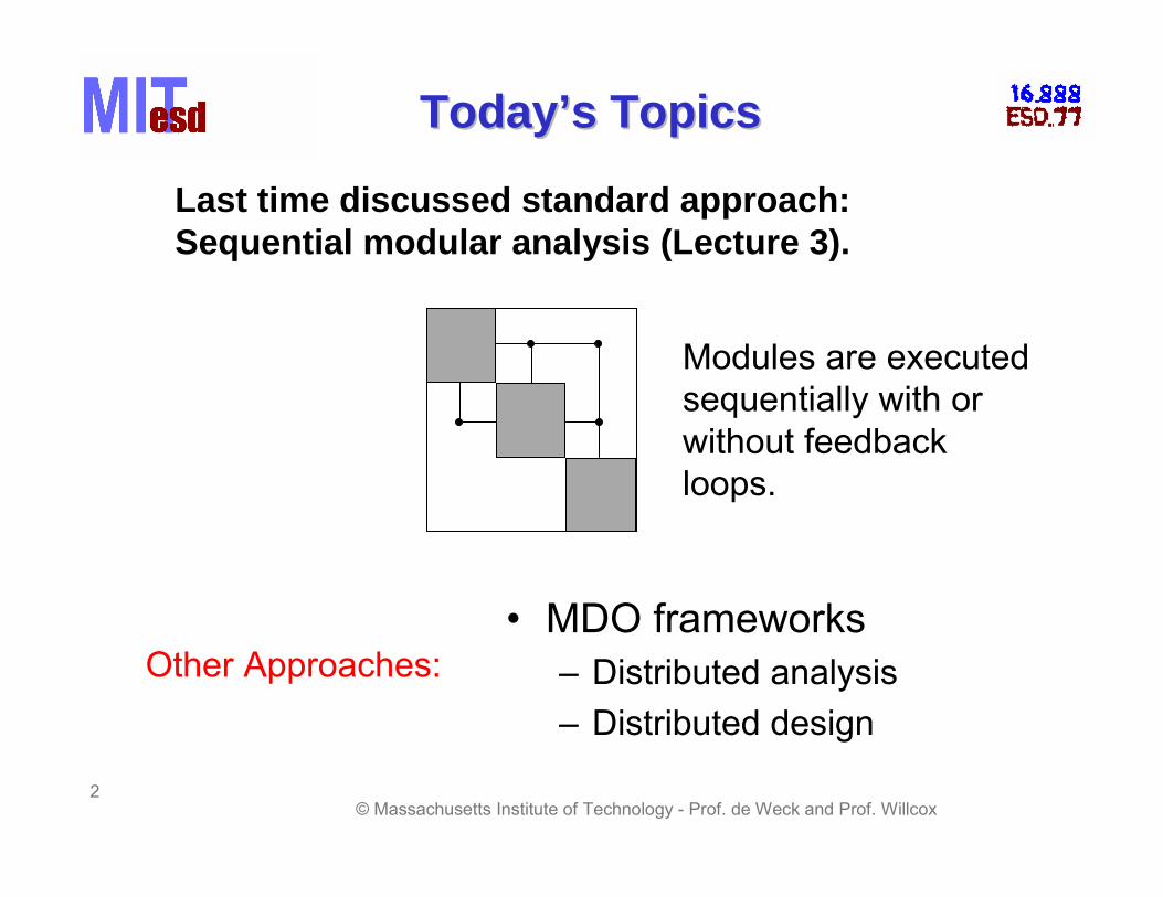
Standard Optimization ProblemStandard Optimization Problem
Given *xx 0
( )J x x ( )g x
Optimization Engine
Function Evaluator
∈ nx ! nJ : ! →
→!
n mg : ! !
Solve the problem
(min J x) (s.t. g x) ≥ 0
* *That is, find x s.t. J( x ) ≤ f x ∀ ∈ J( x), dom( ) ∩dom( )g © Massachusetts Institute of Technology - Prof. de Weck and Prof. Willcox
4

Distributed AnalysisDistributed Analysis• Disciplinary models provide analysis• Optimization is controlled by some overseeing code or database
e.g. GenIE database system (Stanford) ISight (Optimizer) iSight
GenIE NPSol
Shared data
Local data
Structures
Local data
Aero
Optimizer design variables
constraints
x J(x),g(x),h(x)
subsystem analyses
© Massachusetts Institute of Technology - Prof. de Weck and Prof. Willcox 5

Distributed AnalysisDistributed AnalysisOptimizer objective
design variables constraints
x J(x)
performance analysis
aerodynamic analysis
structural analysis
x g(x) h(x) x
g(x) h(x)
• During the optimization, the overseeing code keeps track of the values of the design variables and objective • The values of the design variables are changed according to the optimization algorithm • Disciplinary models are asked to evaluate constraints/objective
© Massachusetts Institute of Technology - Prof. de Weck and Prof. Willcox 6

Distributed DesignDistributed Design
System level optimizer
SS1 optimizer
SS2 optimizer
SSN optimizer
SS1 analyzer
SS2 analyzer
SSN analyzer
……
command/result command/result
command/result
Subsystem black box (BB)
7 © Massachusetts Institute of Technology - Prof. de Weck and Prof. Willcox

Advantages of DecouplingAdvantages of Decoupling
Computation of g(x) can be very time consuming, want to divide the work and compute in parallel.
n2For example, if x = ( ,x x2 ), where x ∈!n1, x ∈!1 1 2
and g(x) = (g x g x ))( ), (1 1 2 2
Then g1 and g2 can be computed in parallel. Graphically,
Optimizer
SS1 SS2
1x 1g 2g x2 g g2
SS1
SS1
Optim 1x 2x
1
© Massachusetts Institute of Technology - Prof. de Weck and Prof. Willcox 8
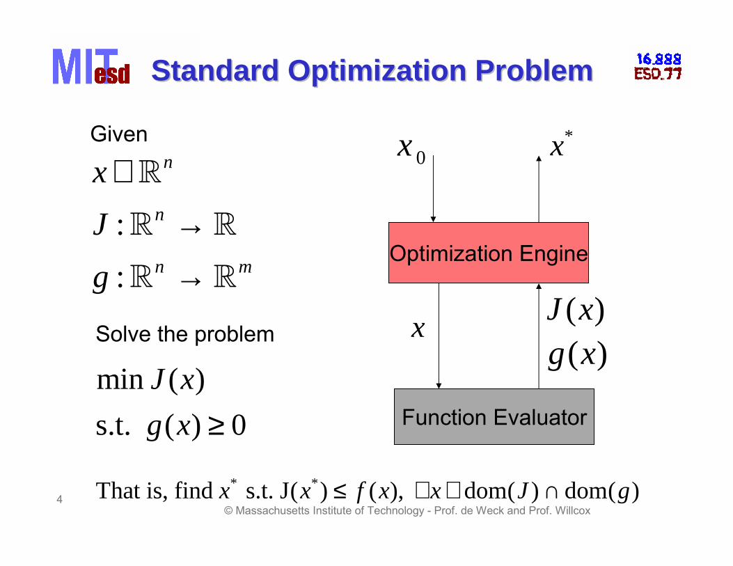
Coupled SituationCoupled Situation The decoupled constraints assumption is not general. Subsystems can be coupled and loops can arise. For example,
Optimizer
SS1 SS2
1x 2x
1u 2u
2w1w SS1
SS2
Optim
1w
2w 1u
1x
2u 2x
1w
2w
Loop
x: decision variables vline: SS inputw: SS outputs (constraint, cost) hline: SS outputu: SS input (dependent)Computation of w1 and w2 requires an iterative method.
© Massachusetts Institute of Technology - Prof. de Weck and Prof. Willcox 9

Information Flow Loop (2)Information Flow Loop (2)
• An example where such a loop happens is as follows:( 1,min J x x2 )
s.t. 1 = ( , 2 ( 2 , 1w g x g x w )) ≥ 01 1
( , ( 1,w2 = g x g x w )) ≥ 02 2 1 2
n2 × i ,where x1 ∈ !n1, x ∈ ! , g : x i " w i = 1, 22 i i
• w1 and w2 satisfy coupled relations at each optimization iteration. At each constraint evaluation, nonlinear equations must be solved (e.g. by Newton’s method) in order to obtain w1 and w , which can2be time consuming.Want a way to return to the situation of decoupled constraints.
© Massachusetts Institute of Technology - Prof. de Weck and Prof. Willcox 10
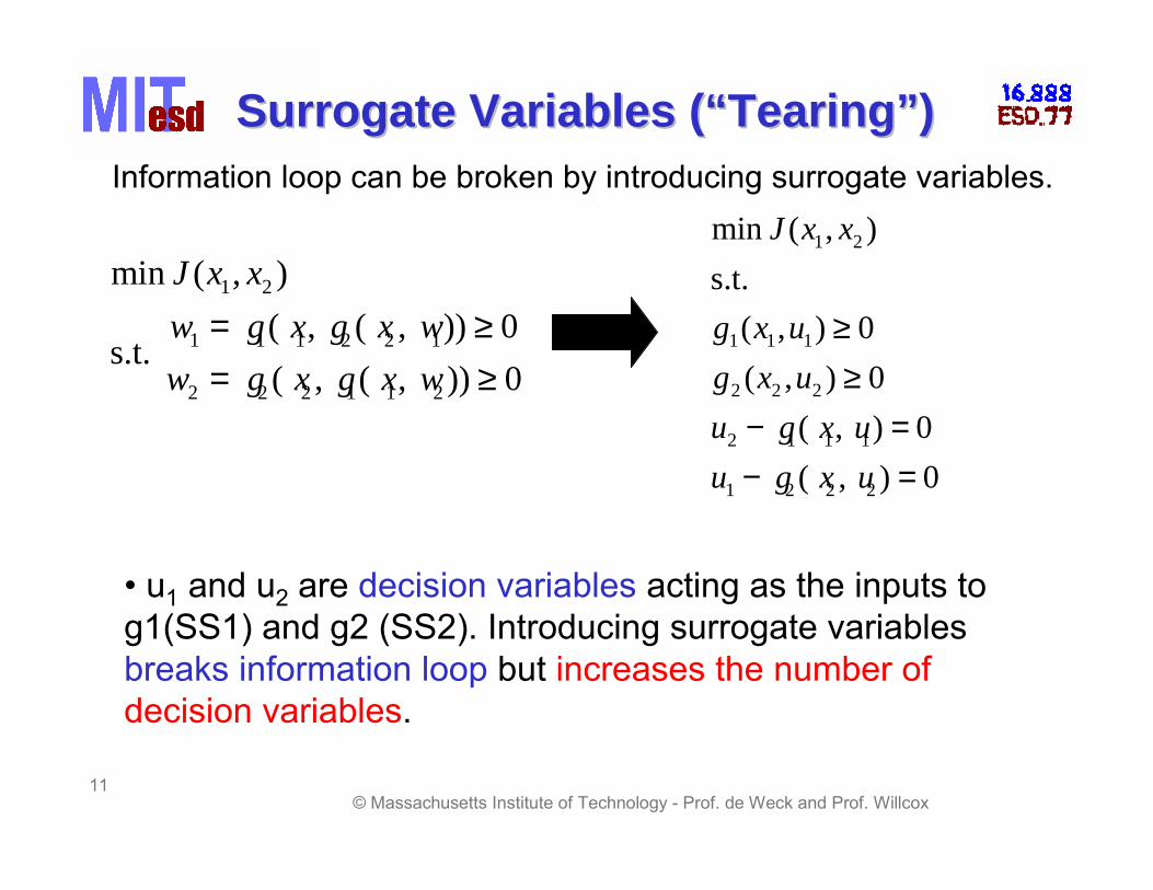
Surrogate Variables (“Tearing”)Surrogate Variables (“Tearing”)Information loop can be broken by introducing surrogate variables.
( 1,min J x x2 ) ( 1,min J x x2 ) s.t.
s.t. 1 = ( , 2 ( 2 , 1w g x g x w )) ≥ 0 ( ,g x u ) ≥ 01 1 1 1 1
( ,g x u ) ≥ 0= ( , ( 1,w g x g x w )) ≥ 02 2 2 1 2 2 2 2
( ,u g x u ) = 02 − 1 1 1
( ,u g x u1 − 2 2 2 ) = 0
• u1 and u2 are decision variables acting as the inputs to g1(SS1) and g2 (SS2). Introducing surrogate variables breaks information loop but increases the number of decision variables.
© Massachusetts Institute of Technology - Prof. de Weck and Prof. Willcox 11

Numerical ExampleNumerical Example
1 + 2 + 2min J J2 decoupled min x x2 + (x − 3)2 + (x − 4)2 1 3 4
s.t. w1 ≥ 0 3s.t. w x x23 + 2x5 ≥ 0= −1 1w2 ≥ 0
3
= 2 + 2 w2 = x x4 + 2x6 ≥ 0− 3
where J x x23
3 − 5 −1J2
1
= (x 1
− 3)2 + (x − 4)2 x x23 + 2x x6 = 0
3 4 3
= 3 − 32
x x43 + 2x x5 = 03w x x2 + 2w − 6 −
1 1
3 − 3w2 = x x4 + 2w3 1 Solution: coupled x = (0, 0, 4, 3,12 , 241
3 )2 3
2 + 2 2 2 MATLAB 5.3min x x2 + (x − 3) + (x − 4)1 3 4
s.t. w g x x x x ) ≥ 0 coupled: 356,423 FLOPS 4.844s= ( 1, 2 , 3,1 1 4
= ( 1, 2 , 3, 4 ) ≥ 0 uncoupled: 281,379 FLOPS 0.453s w g x x x x2 2
© Massachusetts Institute of Technology - Prof. de Weck and Prof. Willcox 12

Distributed Design MethodsDistributed Design Methods • Disciplinary models are provided with design tasks• Optimization is performed at a subsystem level in addition to the system level
Concurrent Subspace Optimization (CSSO)• divide the design problem into several discipline-
related subspaces • each subspace shares responsibility for satisfying
constraints while trying to reduce a global objective
Collaborative Optimization (CO)• disciplinary teams satisfy local constraints while
trying to match target values specified by a system coordinator
• preserves disciplinary-level design freedom
© Massachusetts Institute of Technology - Prof. de Weck and Prof. Willcox 13
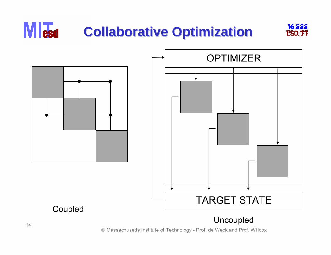
Collaborative OptimizationCollaborative Optimization
OPTIMIZER
TARGET STATE Coupled
Uncoupled14
© Massachusetts Institute of Technology - Prof. de Weck and Prof. Willcox

Collaborative OptimizationCollaborative Optimization
Two levels of optimization:
• A system-level optimizer provides a set of targets.
– These targets are chosen to optimize the system-level objective function
• A subsystem optimizer finds a design that minimizes the difference between current states and the targets.
– Subject to local constraints
© Massachusetts Institute of Technology - Prof. de Weck and Prof. Willcox 15
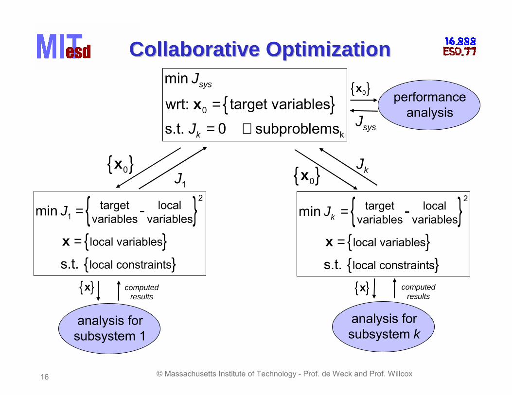
Collaborative OptimizationCollaborative Optimizationmin Jsys {x0} wrt: x0 = {target variables}
syss.t. Jk = 0 ∀ subproblems J
performance analysis
k
{x0} J1
{x0} Jk
2 2local localmin J1 = target - {variables variables}{variables variables} min Jk = target
x = {local variables} x = {local variables} s.t. {local constraints} s.t. {local constraints}
analysis for subsystem 1
analysis for subsystem k
{x} computed {x} computed results results
© Massachusetts Institute of Technology - Prof. de Weck and Prof. Willcox 16
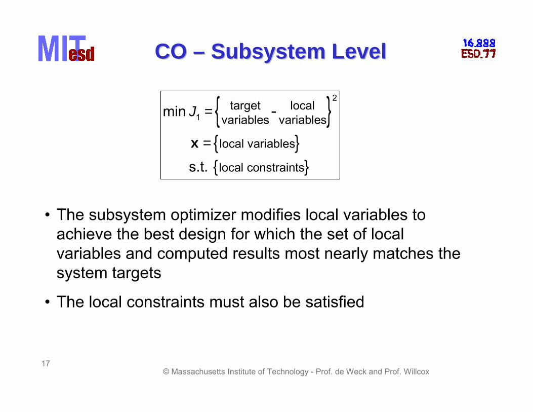
COCO –– Subsystem LevelSubsystem Level
2localmin J1 = target {variables variables}
x = {local variables} s.t. {local constraints}
• The subsystem optimizer modifies local variables to achieve the best design for which the set of local variables and computed results most nearly matches the system targets
• The local constraints must also be satisfied
© Massachusetts Institute of Technology - Prof. de Weck and Prof. Willcox 17

COCO –– System LevelSystem Levelmin Jsys
wrt: x0 = {target variables} s.t. Jk = 0 ∀ subproblemsk
• System-level optimizer changes target variables to improve objective and reduce differences Jk
– Jk=0 are called compatibility constraints
– compatibility constraints are driven to zero, but may be violated during the optimization
– CO may therefore discover parts of the design space that cannot be reached by sequential optimization
© Massachusetts Institute of Technology - Prof. de Weck and Prof. Willcox 18

CO Example: Aircraft DesignCO Example: Aircraft DesignConsider a simple aircraft design problem:maximize range for a given take-off weight by choosing wing area, aspect ratio, twist angle, L/D, and wing weight.
aero
struct
perfmodified from Kroo et al. AIAA 94-4325
wing area, S aspect ratio, AR
twist angle, θ
range, R
L/D
wing weight, W
© Massachusetts Institute of Technology - Prof. de Weck and Prof. Willcox 19

x
CO Example: Aircraft DesignCO Example: Aircraft Designmax R0
Tx0 = [R0 S0 AR0 θ0 L/D0 W0]s.t. J1=0, J2=0, J3=0
x0 J1
x0 J2
min J2 J2= (AR-AR0)2 + (θ-θ0)2+
2(S-S0)2 + (W-W0)Tx = [S AR]
x θ, W
struct analysis
x0 J3
min J3 J3= (R-R0)2 + (L/D-L/D0)
2+ (W-W0)Tx = [L/D W]
x R
perf analysis
min J1 J1= (AR-AR0)2 + (θ-θ0)2+
2(L/D-L/D0)2 + (S-S0)Tx = [AR θ]
L/D
aero analysis
© Massachusetts Institute of Technology - Prof. de Weck and Prof. Willcox 20
2
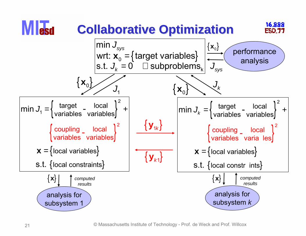
Collaborative OptimizationCollaborative Optimizationmin Jsys {x0}wrt: x0 = {target variables}s.t. Jk = 0 ∀ subproblems Jsysk
performance analysis
{x0} J1 {x0} Jk
2 2local localmin J1 = target - + min Jk = target - +{variables variables} {variables variables} 2 2 coupling local coupling local- -{variables variables}
{ }
{y1k } {variables varia les} x = {local variables} x = {local variables} s.t. {local constraints}
yk1 s.t. {local constr in s}t
computed
analysis for subsystem 1
{x} computed {x}resultsresults
analysis for subsystem k
© Massachusetts Institute of Technology - Prof. de Weck and Prof. Willcox 21

Collaborative OptimizationCollaborative Optimization
y
x0 = system-level target variable values
x = subsystem local variables
ij = coupling functions
• yij =outputs of subsystem j which are needed as inputs to subsystem i.
• Coupling equations must also be satisfied, so coupling variables are included in subsystem objective.
• Used to reduce the number of system-level parameters.
© Massachusetts Institute of Technology - Prof. de Weck and Prof. Willcox 22
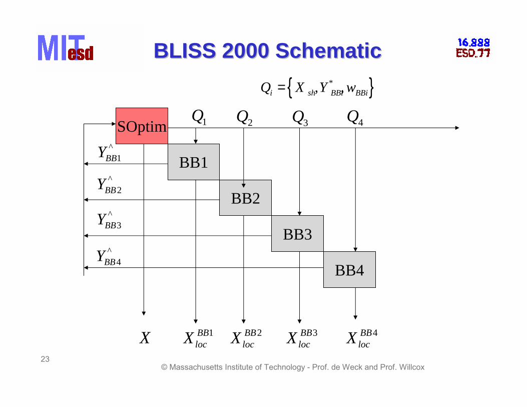
BLISS 2000 SchematicBLISS 2000 SchematicQ = {X ,Y *
BBi }i sh BBi , w
SOptim
BB1
BB2
BB3
BB4
^ 1BBY
^ 2BBY
^ 3BBY
^ 4BBY
1Q 2Q 3Q 4Q
BB1 BB2 BB3 BB4X Xloc X loc X loc X loc
23© Massachusetts Institute of Technology - Prof. de Weck and Prof. Willcox

Black Box (BB)Black Box (BB)
A black box has the following properties:
1. BB has its own local variables (Xloc) and has the exclusive right to determine Xloc. Xloc is a subset of decision variables that can appear explicitly only in the associated BB.
2. BB must satisfies its constraints at each system level iteration.
3. BB operates independently of other BB’s. Neither its inputs nor its outputs are directly communicated between other BB’s. Also, BB assumes no knowledge (e.g. Xloc) of other BB’s. Instead, BB connection is done implicitly via the system optimizer, by the use of Y*.
4. Computation methods within a BB are not restricted by BLISS. (It can be simulation or just an intelligent guess.)
© Massachusetts Institute of Technology - Prof. de Weck and Prof. Willcox 24
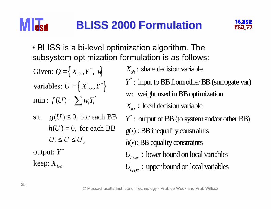
BLISS 2000 FormulationBLISS 2000 Formulation
• BLISS is a bi-level optimization algorithm. The subsystem optimization formulation is as follows:
*Given: Q = {X , Y w} Xsh : share decision variable sh ,
variables: U = {Xloc , Y ^ } Y* : input to BB from other BB (surrogate var)
min : f U ) =∑ wY w: weight used in BB optimization
( ^ i i Xloc : local decision variablei
(s.t. g U ) ≤ 0, for each BB Y^ : output of BB (to system and/or other BB) (h U ) = 0, for each BB g(i) : BB inequali y constraints
UUl ≤ ≤ Uu h(i): BB equality constraints output: Y ^
Ulower : lower bound on local variables keep: Xloc U : upper bound on local variablesupper
© Massachusetts Institute of Technology - Prof. de Weck and Prof. Willcox 25
InsertInsert –– Slides by Dr. SobieskiSlides by Dr. Sobieski
26© Massachusetts Institute of Technology - Prof. de Weck and Prof. Willcox

Wing drag and weight both influence the flight range R.R is the system objective
• direct • i
P P
Displ
a
li
that affect drag Displ
Wing - structure Wing - aerodynamics Loads
acements
a = sweep angle
• Structure influences R byy by weight
ndirectly by st ffness that affect displacements Loads & acements
must be consistent
R = (k/Drag) LOG [( Wo + Ws + Wf)/ (Wo + Ws )]
• Dilemma: What to optimize the structure for? Lightness? Displacements = 1/Stiffness?
An optimal mix of the two?
Courtesy of Jaroslaw Sobieski. Used with permission.

Trade-off between opposing objectivesof lightness and stiffness
Weight Displacement Weight
Displacement ~ 1/Stiffness
Thickness limited by stress
Wing cover sheet thickness
Lightness Stiffness
• What to optimize for? • Answer: minimum of f = w1 Weight + w2 Displacement• vary w1, w2 to generate a population of wings of diverse Weight/Displacement ratios • Let system choose w1, w2.
Courtesy of Jaroslaw Sobieski. Used with permission.
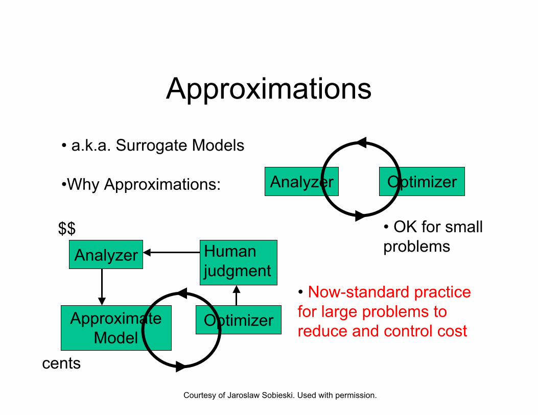
Approximations
•Why Approximations: Analyzer
Analyzer
Approximate Model
Human judgment
problems
• ice for large problems to reduce and control cost
$$
cents
• a.k.a. Surrogate Models
Optimizer
Optimizer
• OK for small
Now-standard pract
Courtesy of Jaroslaw Sobieski. Used with permission.
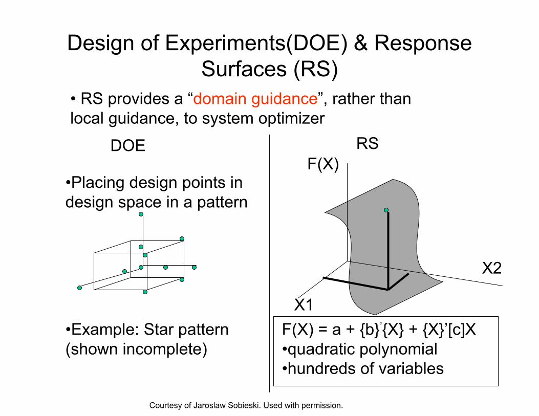
Design of Experiments(DOE) & ResponseSurfaces (RS)
• RS provides a —domain guidance“, rather than local guidance, to system optimizer
DOE
•Placing design points indesign space in a pattern
•Example: Star pattern (shown incomplete)
RS
X1
X2
F(X)
F(X) = a + {b}‘{X} + {X}‘[c]X •quadratic polynomial •hundreds of variables
Courtesy of Jaroslaw Sobieski. Used with permission.
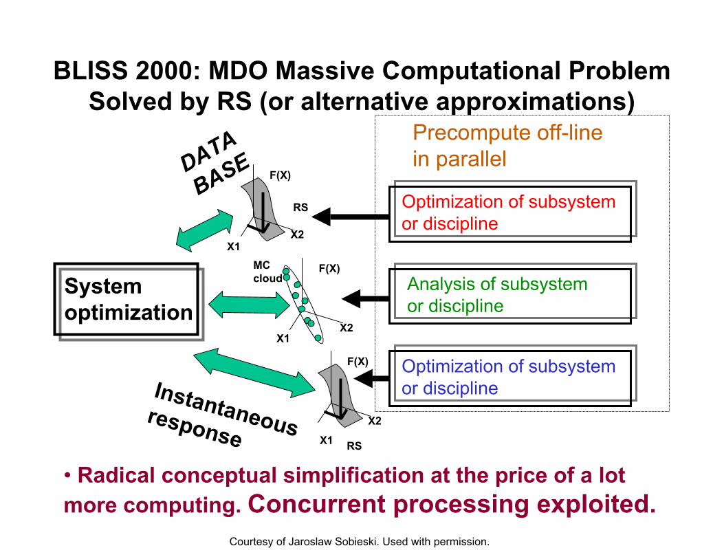
BLISS 2000: MDO Massive Computational ProblemSolved by RS (or alternative approximations)
or di
or di
or di
System optimization
X1 X2
)
X1 X2
)
X1
X2
)
RS
RS
ine in parallel
Instantaneousresponse
MC
DATA
BASE
Optimization of subsystem scipline
Analysis of subsystem scipline
Optimization of subsystem scipline
F(X
F(X
F(X
Precompute off-l
cloud
• Radical conceptual simplification at the price of a lot more computing. Concurrent processing exploited.
Courtesy of Jaroslaw Sobieski. Used with permission.

Coupled System Sensitivity
• Consider a multidisciplinary YAsystem with two subsystems X A and B (e.g. Aero. & Struct.) œ system equations can be
written in symboli[(X A A ,Y ),Y ] = 0B A
B [( X ,Y ),Y ] = 0B A B
œ rewrite these as followsYA = YA ( X ,Y )A B
YB = YB ( X ,YA )B
A
B
A
BX
BY
BYAYc form as
these governing equations define
as implicit functions. Implicit Function Theorem applies.
Courtesy of Jaroslaw Sobieski. Used with permission.
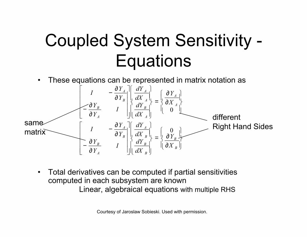
Coupled System Sensitivity -Equations
• These equations can be represented in matrix notation asY dY
dX
∂∂
=
A A
A
I − YA
X
∂∂ A
YB
Y dY∂∂
B BI− 0Y dX differentA A
same Y dY∂∂
Right Hand SidesA AI − 0=
matrix
Y dX Y∂
∂X
B B BY dY
dX
∂∂
B B
B
I− BY A
• Total derivatives can be computed if partial sensitivitiescomputed in each subsystem are known
Linear, algebraical equations with multiple RHS
Courtesy of Jaroslaw Sobieski. Used with permission.
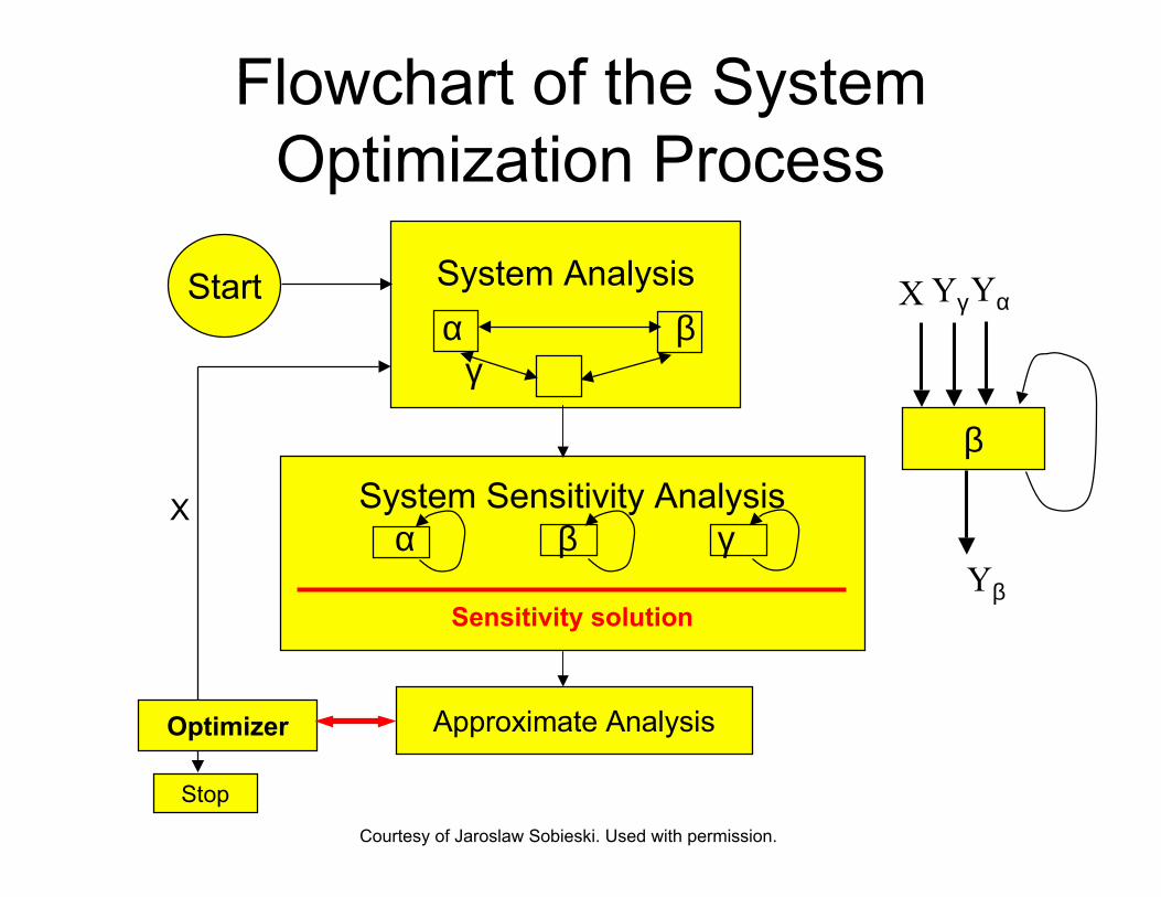
X
Flowchart of the SystemOptimization Process
System Analysis α β
γ
System Sensitivity Analysis α β γ
Start
Sensitivity solution
Approximate Analysis Optimizer
X Yγ Yα
β
Yβ
Stop
Courtesy of Jaroslaw Sobieski. Used with permission.

System Internal CouplingsC
oupl
ing
Brea
d th
Quantified
All-in-One
Decompose
((Decompose))
(Decompose)
• Strength: relatively large ∂ YO/ ∂YI
• Breadth: {YO} and {YI} are long
[∂ YO/ ∂YI] large and full
Coupling Strength
Courtesy of Jaroslaw Sobieski. Used with permission.

Supersonic Business Jet Test Case
• Structures (ELAPS)
• )
• )
• )
Aerodynamics (lift, drag, trim supersonic wave drag by A - Wave
Propulsion (look-up tables
Performance (Breguet equation for Range
Some stats:
Xlocal: struct. 18aero 3propuls. 1
X shared: 9Y coupl.: 9
Examples: Xsh - wing aspect ratio, Engine scale factor Xloc - wing cover thickness, throttle setting Y - aerodynamic loads, wing deformation.
Courtesy of Jaroslaw Sobieski. Used with permission.

System of Modules (Black Boxes) for Supersonic Business Jet Test Case
Struct.
Perform.
Aero
Propulsion
• Data Dependence Graph • RS - quadratic polynomials, adjusted for error control
Courtesy of Jaroslaw Sobieski. Used with permission.
0
1
1 10
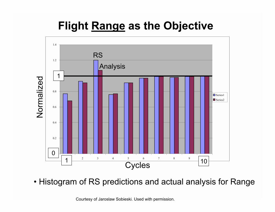
Flight Range as the ObjectiveN
orm
aliz
ed
Cycles
0.2
0.4
0.6
0.8
1.2
1.4
2 3 4 5 6 7 8 9
Series1
Series2
RS
1
101 0
Analysis
• Histogram of RS predictions and actual analysis for Range
Courtesy of Jaroslaw Sobieski. Used with permission.

References (I)References (I)
Jaroslaw, Sobieszczanski-Sobieski et al. Bi-level Intergrated System Synthesis (BLISS) For Concurrent And Distributed Processing. AIAA 2002-5409.
Updated Journal Article (handout): Jaroslaw Sobieski, Altus, Phillips, Sandusky, “Bi-level Integrated System
Synthesis for Concurrent and Distributed Processing” AIAA Journal, Vol. 41, No.10, October 2003, pp. 1996-2003
I.P. Sobieski and I.M. Kroo. Collaborative Optimization Using Response Surface Estimation. AIAA Journal Vol. 38 No. 10. Oct 2000.
R.D. Braun and I.M. Kroo. Development and Application of the Collaborative Optimization Architecture in a Multidisciplinary Design Environment. ICASE/NASA Langley Workshop on MDO, March 13-16, 1995
Erin J. Cramer et al. Problem Formulation for Multidisciplinary Optimization. SIAM Journal of Optimization. Vol. 4, No. 4 pp. 754-776, Nov 1994
Natalia M. Alexandrov (ed). Multidisciplinary Design Optimization – State of the Art. SIAM. 1994.
© Massachusetts Institute of Technology - Prof. de Weck and Prof. Willcox 27

References (II)References (II)
Kroo, I.: “MDO applications in preliminary design: status and directions,” AIAA Paper 97-1408, 1997.
Kroo, I. and Manning, V.: “Collaborative optimization: status and directions,” AIAA Paper 2000-4721, 2000.
Sobieski, I. and Kroo, I.: “Aircraft design using collaborative optimization,” AIAA Paper 96-0715, 1996.
Balling, R. and Wilkinson, C.: “Execution of multidisciplinary design optimization approaches on common test problems,” AIAA Paper 964033, 1996.
Giesing, J. and Barthelemy, J.: “A summary of industry MDO applications and needs”, AIAA White Paper, 1998.
AIAA MDO Technical Committee: “Current state-of-the-art in multidisciplinary design optimization”, 1991.
“Optimal Design in Multidisciplinary Systems,” AIAA Professional Development Short Course Notes, September 2002.
© Massachusetts Institute of Technology - Prof. de Weck and Prof. Willcox 28