Multicriteria Optimization andDecision Making

Principles, Algorithms and Case Studies

Michael Emmerich and Andre DeutzLIACS Master Course: Autumn/Winter 2014/2015

Contents

1 Introduction 51.1 Viewing mulicriteria optimization as a task in system design and

analysis . . . . . . . . . . . . . . . . . . . . . . . . . . . . . . . . . 71.2 Formal Problem Definitions . . . . . . . . . . . . . . . . . . . . . . 9

1.2.1 Other Problem Classes in Optimization . . . . . . . . . . . . 101.2.2 Multiobjective Optimization . . . . . . . . . . . . . . . . . . 11

1.3 Problem Difficulty in Optimization . . . . . . . . . . . . . . . . . . 121.3.1 Problem Difficulty in Continuous Optimization . . . . . . . 121.3.2 Problem Difficulty in Combinatorial Optimization . . . . . . 14

1.4 Pareto dominance and incomparability . . . . . . . . . . . . . . . . 171.5 Formal Definition of Pareto Dominance . . . . . . . . . . . . . . . . 19

I Foundations 21

2 Orders and dominance 222.1 Preorders . . . . . . . . . . . . . . . . . . . . . . . . . . . . . . . . 222.2 Preorders . . . . . . . . . . . . . . . . . . . . . . . . . . . . . . . . 232.3 Partial orders . . . . . . . . . . . . . . . . . . . . . . . . . . . . . . 252.4 Linear orders and anti-chains . . . . . . . . . . . . . . . . . . . . . 262.5 Hasse diagrams . . . . . . . . . . . . . . . . . . . . . . . . . . . . . 262.6 Comparing ordered sets . . . . . . . . . . . . . . . . . . . . . . . . 282.7 Cone orders . . . . . . . . . . . . . . . . . . . . . . . . . . . . . . . 29

3 Landscape Analysis 343.1 Search Space vs. Objective Space . . . . . . . . . . . . . . . . . . . 343.2 Global Pareto Fronts and Efficient Sets . . . . . . . . . . . . . . . . 363.3 Weak efficiency . . . . . . . . . . . . . . . . . . . . . . . . . . . . . 373.4 Characteristics of Pareto Sets . . . . . . . . . . . . . . . . . . . . . 383.5 Optimality conditions based on level sets . . . . . . . . . . . . . . . 393.6 Local Pareto Optimality . . . . . . . . . . . . . . . . . . . . . . . . 41

1

3.7 Barrier Structures . . . . . . . . . . . . . . . . . . . . . . . . . . . . 433.8 Shapes of Pareto Fronts . . . . . . . . . . . . . . . . . . . . . . . . 463.9 Conclusions . . . . . . . . . . . . . . . . . . . . . . . . . . . . . . . 49

4 Optimality conditions for differentiable problems 504.1 Linear approximations . . . . . . . . . . . . . . . . . . . . . . . . . 504.2 Unconstrained Optimization . . . . . . . . . . . . . . . . . . . . . . 504.3 Equality Constraints . . . . . . . . . . . . . . . . . . . . . . . . . . 524.4 Inequality Constraints . . . . . . . . . . . . . . . . . . . . . . . . . 554.5 Multiple Objectives . . . . . . . . . . . . . . . . . . . . . . . . . . . 57

5 Scalarization Methods 595.1 Linear Aggregation . . . . . . . . . . . . . . . . . . . . . . . . . . . 605.2 Nonlinear Aggregation . . . . . . . . . . . . . . . . . . . . . . . . . 625.3 Multi-Attribute Utility Theory . . . . . . . . . . . . . . . . . . . . . 625.4 Distance to a Reference Point Methods . . . . . . . . . . . . . . . . 67

6 Transforming Multicriteria into Constrained Single-Criterion Prob-lems 716.1 Compromise Programming or ε-Constraint Methods . . . . . . . . . 716.2 Concluding remarks on single point methods . . . . . . . . . . . . . 73

II Algorithms for Pareto Optimization 76

7 Pareto Front Computing with Deterministic Methods 777.1 Computing the Maximal Set of Vectors . . . . . . . . . . . . . . . . 77

8 Evolutionary Multicriterion Optimization 818.1 Single Objective Evolutionary Algorithms . . . . . . . . . . . . . . 828.2 Evolutionary Multiobjective Optimization . . . . . . . . . . . . . . 86

8.2.1 Algorithms Balancing Dominance and Diversity . . . . . . . 888.2.2 Indicator-based Algorithms . . . . . . . . . . . . . . . . . . 898.2.3 Multiobjective Evolution Strategy . . . . . . . . . . . . . . . 92

8.3 Final Remarks . . . . . . . . . . . . . . . . . . . . . . . . . . . . . . 93

9 Conclusion 94

2

Preface

Finding optimal solutions in large and constrained search spaces has been sincelong the core topic of operations research and engineering optimization. Suchproblems are typically challenging from an algorithmic point of view. Multicriteriaoptimization can be seen as a modern variant of it, that also takes into accountthat in real world problems we also have to deal with multicriteria decision makingand the aspect of searching for an optimum should be combined with aspectsof multicriteria decision analysis (MCDA), which is the science of making goodchoices based on the systematic analysis of alternatives:

Real world decision and optimization problems usually involve conflicting cri-teria. Think of chosing a means to travel from one country to another. It shouldbe fast, cheap or convenient, but you probably cannot have it all. Or you wouldlike to design an industrial process, that should be safe, environmental friendlyand cost efficient. Ideal solutions, where all objectives are at their optimal level,are rather the exception than the rule. Rather we need to find good compromises,and avoid lose-lose situations.

These lecture nodes deal with Multiobjective Optimization and Decision Anal-ysis (MODA). We define this field, based on some other scientific disciplines:

DEF Multicriteria Decision Aiding (MCDA) (or: Multiattribute Decision Analy-sis) is a scientific field that studies evaluation of a finite number of alterna-tives based on multiple criteria. It provides methods to compare, evaluate,and rank solutions.

DEF Multicriteria Optimization (MCO) (or: Multicriteria Design, MulticriteriaMathematical Programming) is a scientific field that studies search for op-timal solutions given multiple criteria and constraints. Here, usually, thesearch space is very large and not all solutions can be inspected.

DEF Multicriteria Decision Making (MCDM) deals with MCDA and MCO orcombinations of these.

We use here the title: Multicriteria Optimization and Decision Analysis =MODA as a synonym of MCDM in order to focus more on the algorithmicallychallenging optimization aspect.

3

In this course we will deal with algorithmic methods for solving (constrained)multi-objective optimization and decision making problems. The rich mathemati-cal structure of such problems as well as their high relevance in various applicationfields led recently to a significant increase of research activities. In particular al-gorithms that make use of fast, parallel computing technologies are envisaged fortackling hard combinatorial and/or nonlinear application problems. In the coursewe will discuss the theoretical foundations of multi-objective optimization prob-lems and their solution methods, including order and decision theory, analytical,interactive and meta-heuristic solution methods as well as state-of-the-art tools fortheir performance-assessment. Also an overview on decision aid tools and formalways to reason about conflicts will be provided. All theoretical concepts will beaccompanied by illustrative hand calculations and graphical visualizations duringthe course. In the second part of the course, the discussed approaches will be ex-emplified by the presentation of case studies from the literature, including variousapplication domains of decision making, e.g. economy, engineering, medicine orsocial science.

This reader is covering the topic of Multicriteria Optimization and DecisionMaking. Our aim is to give a broad introduction to the field, rather than tospecialize on certain types of algorithms and applications. Exact algorithms forsolving optimization algorithms are discussed as well as selected techniques fromthe field of metaheuristic optimization, which received growing popularity in recentyears. The lecture notes provides a detailed introduction into the foundations anda starting point into the methods and applications for this exciting field of inter-disciplinary science. Besides orienting the reader about state-of-the-art techniquesand terminology, references are given that invite the reader to further reading andpoint to specialized topics.

4

Chapter 1

Introduction

For several reasons multicriteria optimization and decision making is an excitingfield of computer science and operations research. Part of its fascination stems fromthe fact that in MCO and MCDM different scientific fields are addressed. Firstly,to develop the general foundations and methods of the field one has to deal withstructural sciences, such as algorithmics, relational logic, operations research, andnumerical analysis:

• How can we state a decision/optimization problem in a formal way?

• What are the essential differences between single objective and multiobjec-tive optimization?

• How can we rank solutions? What different types of orderings are used indecision theory and how are they related to each other?

• Given a decision model or optimization problem, which formal conditionsneed to be satisfied for solutions to be optimal?

• How can we construct algorithms that obtain optimal solutions, or approxi-mations to them, in an efficient way?

• What is the geometrical structure of solution sets for problems with morethan one optimal solution?

Whenever it comes to decision making in the real world, these decisions willbe made by people responsible for it. In order to understand how people cometo decisions and how the psychology of individuals (cognition, individual decisionmaking) and organizations (group decision making) needs to be studied. Questionslike the following may arise:

5

• What are our goals? What makes it difficult to state goals? How do peopledefine goals? Can the process of identifying goals be supported?

• Which different strategies are used by people to come to decisions? Howcan satisfaction be measured? What strategies are promising in obtainingsatisfactory decisions?

• What are the cognitive aspects in decision making? How can decision supportsystems be build in a way that takes care of cognitive capabilities and limitsof humans?

• How do groups of people come to decisions? What are conflicts and how canthey be avoided? How to deal with minority interests in a democratic decisionprocess? Can these aspects be integrated into formal decision models?

Moreover, decisions are always related to some real world problem. Given anapplication field, we may find very specific answers to the following questions:

• What is the set of alternatives?

• By which means can we retrieve the values for the criteria (experiments,surveys, function evaluations)? Are there any particular problems with thesemeasurements (dangers, costs), and how to deal with them? What are theuncertainties in these measurements?

• What are the problem-specific objectives and constraints?

• What are typical decision processes in the field, and what implications dothey have for the design of decision support systems?

• Are there existing problem-specific procedures for decision support and op-timization, and what about the acceptance and performance of these proce-dures in practice?

In summary, this list of questions gives some kind of bird’s eye view of the field.However, in these lecture notes we will mainly focus on the structural aspects ofmulti-objective optimization and decision making. On the other hand, we alsodevote one chapter to human-centric aspects of decision making and one chapterto the problem of selecting, adapting, and evaluating MOO tools for applicationproblems.

6

1.1 Viewing mulicriteria optimization as a task

in system design and analysis

The discussion above can be seen as a rough sketch of questions that define thescope of multicriteria optimization and decision making. However, it needs to beclarified more precisely what is going to be the focus of these lecture notes. Forthis reason we want to approach the problem class from the point of view of systemdesign and analysis. Here, with system analysis, we denote the interdisciplinaryresearch field, that deals with the modeling, simulation, and synthesis of complexsystems.

Beside experimentation with a physical system, often a system model is used.Nowadays, system models are typically implemented as computer programs thatsolve (differential) equation systems, simulate interacting automata, or stochasticmodels. We will also refer to them as simulation models. An example for asimulation model based on differential equations would be the simulation of thefluid flow around an airfoil based on the Navier Stokes equations. An example fora stochastic system model, could be the simulation of a system of elevators, basedon some agent based stochastic model.

?

!

!

! !

!

!

!

!

!

!

!

!

!

?

?

?

!

?

?

?

Calibration

Identification

Modelling

Simulation

Prediction

Exploration

Optimization

Inverse Design

Control*

*) if system (model) is dynamic

Figure 1.1: Different tasks in systems analysis.

In Figure 1.1 different tasks of systems analysis based on simulation models aredisplayed in a schematic way. Modeling means to identify the internal structure ofthe simulation model. This is done by looking at the relationship between known

7

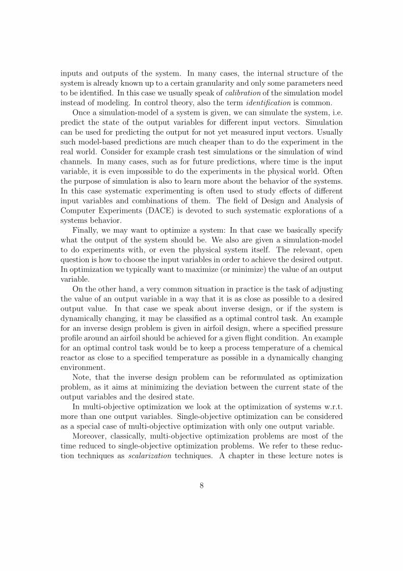
inputs and outputs of the system. In many cases, the internal structure of thesystem is already known up to a certain granularity and only some parameters needto be identified. In this case we usually speak of calibration of the simulation modelinstead of modeling. In control theory, also the term identification is common.

Once a simulation-model of a system is given, we can simulate the system, i.e.predict the state of the output variables for different input vectors. Simulationcan be used for predicting the output for not yet measured input vectors. Usuallysuch model-based predictions are much cheaper than to do the experiment in thereal world. Consider for example crash test simulations or the simulation of windchannels. In many cases, such as for future predictions, where time is the inputvariable, it is even impossible to do the experiments in the physical world. Oftenthe purpose of simulation is also to learn more about the behavior of the systems.In this case systematic experimenting is often used to study effects of differentinput variables and combinations of them. The field of Design and Analysis ofComputer Experiments (DACE) is devoted to such systematic explorations of asystems behavior.

Finally, we may want to optimize a system: In that case we basically specifywhat the output of the system should be. We also are given a simulation-modelto do experiments with, or even the physical system itself. The relevant, openquestion is how to choose the input variables in order to achieve the desired output.In optimization we typically want to maximize (or minimize) the value of an outputvariable.

On the other hand, a very common situation in practice is the task of adjustingthe value of an output variable in a way that it is as close as possible to a desiredoutput value. In that case we speak about inverse design, or if the system isdynamically changing, it may be classified as a optimal control task. An examplefor an inverse design problem is given in airfoil design, where a specified pressureprofile around an airfoil should be achieved for a given flight condition. An examplefor an optimal control task would be to keep a process temperature of a chemicalreactor as close to a specified temperature as possible in a dynamically changingenvironment.

Note, that the inverse design problem can be reformulated as optimizationproblem, as it aims at minimizing the deviation between the current state of theoutput variables and the desired state.

In multi-objective optimization we look at the optimization of systems w.r.t.more than one output variables. Single-objective optimization can be consideredas a special case of multi-objective optimization with only one output variable.

Moreover, classically, multi-objective optimization problems are most of thetime reduced to single-objective optimization problems. We refer to these reduc-tion techniques as scalarization techniques. A chapter in these lecture notes is

8

devoted to this topic. Modern techniques, however, often aim at obtaining a set of’interesting’ solutions by means of so-called Pareto optimization techniques. Whatis meant by this will be discussed in the remainder of this chapter.

1.2 Formal Problem Definitions in Mathematical

Programming

Researchers in the field of operations research use an elegant and standardized nota-tion for the classification and formalization of optimization and decision problems,the so-called mathematical programming problems, among which linear programs(LP) are certainly the most prominent representant. Using this notion a genericdefinition of optimization problems is as follows:

f(x) → min! (* Objectives *) (1.1)

g1(x) ≤ 0 (* Inequality constraints *) (1.2)... (1.3)

gng(x) ≤ 0 (1.4)

h1(x) = 0 (* Equality Constraints *) (1.5)... (1.6)

hnh(x) = 0 (1.7)

x ∈ X = [xmin,xmax] ⊂ Rnx × Znz (* Box constraints *) (1.8)

(1.9)

The objective function f is a function to be minimized (or maximized1). Thisis the goal of the optimization. The function f can be evaluated for every point xin the search space (or decision space). Here the search space is defined by a set ofintervals, that restrict the range of variables, so called bounds or box constraints.Besides this, variables can be integer variables that is they are chosen from Z orsubsets of it, or continuous variable (from R). An important special case of integervariables are binary variables which are often used to model binary decisions inmathematical programming.

Whenever inequality and equality constraints are stated explicitly, the searchspace X can be partitioned in a feasible search space Xf ⊆ X and an infeasiblesubspace X − Xf . In the feasible subspace all conditions stated in the mathe-matical programming problem are satisfied. The conditions in the mathematical

1Maximization can be rewritten as minimization by changing the sign of the objective func-tion, that is, replacing f(x)→ max with −f(x)→ min

9

program are used to avoid constraint violations in the system under design, e.g.,the excess of a critical temperature or pressure in a chemical reactor (an examplefor an inequality constraint), or the keeping of conservation of mass formulatedas an equation (an example for an equality constraint). The conditions are calledconstraints. Due to a convention in the field of operations research, constraintsare typically written in a standardized form such that 0 appears on the right handside side. Equations can easily be transformed into the standard form by meansof algebraic equivalence transformations.

Based on this very general problem definition we can define several classes ofoptimization problems by looking at the characteristics of the functions f , gi, i =1, . . . , ng, and hi, i = 1, . . . , nh. Some important classes are listed in Table 1.1.

Name Abbreviation Search Space FunctionsLinear Program LP Rnr linearQuadratic Program QP Rnr quadraticInteger Linear Progam ILP Znz linearInteger Progam IP Znz arbitraryMixed Integer Linear Program MILP Znz × Rnr linearMixed Integer Nonlinear Program MINLP Znz × Rnr nonlinear

Table 1.1: Classification of mathematical programming problems.

1.2.1 Other Problem Classes in Optimization

There are also other types of mathematical programming problems. These are, forinstance based on:

• The handling of uncertainties and noise of the input variables and of theparameters of the objective function: Such problems fall into the class ofrobust optimization problems and stochastic programming. If some of theconstants in the objective functions are modeled as stochastic variables thecorresponding problems are also called a parametric optimization problem.

• Non-standard search spaces: Non-standard search spaces are for instance thesearch spaces of trees (e.g. representing regular expressions), network config-urations (e.g. representing flowsheet designs) or searching for 3-D structures(e.g. representing bridge constructions). Such problem are referred to astopological, grammatical, or structure optimization.

• A finer distinction between different mathematical programming problemsbased on the characteristics of the functions: Often subclasses of mathe-matical programming problems have certain mathematical properties that

10

can be exploited for faster solving them. For instance convex quadratic pro-gramming problems form a special class of relatively easy to solve quadraticprogramming problems. Moreover, geometrical programming problems are animportant subclass of nonlinear programming tasks with polynomials thatare allowed to h negative numbers or fractions as exponents.

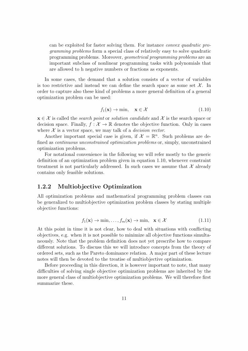
In some cases, the demand that a solution consists of a vector of variablesis too restrictive and instead we can define the search space as some set X . Inorder to capture also these kind of problems a more general definition of a generaloptimization problem can be used:

f1(x)→ min, x ∈ X (1.10)

x ∈ X is called the search point or solution candidate and X is the search space ordecision space. Finally, f : X → R denotes the objective function. Only in caseswhere X is a vector space, we may talk of a decision vector.

Another important special case is given, if X = Rn. Such problems are de-fined as continuous unconstrained optimization problems or, simply, unconstrainedoptimization problems.

For notational convenience in the following we will refer mostly to the genericdefinition of an optimization problem given in equation 1.10, whenever constrainttreatment is not particularly addressed. In such cases we assume that X alreadycontains only feasible solutions.

1.2.2 Multiobjective Optimization

All optimization problems and mathematical programming problem classes canbe generalized to multiobjective optimization problem classes by stating multipleobjective functions:

f1(x)→ min, . . . , fm(x)→ min, x ∈ X (1.11)

At this point in time it is not clear, how to deal with situations with conflictingobjectives, e.g. when it is not possible to minimize all objective functions simulta-neously. Note that the problem definition does not yet prescribe how to comparedifferent solutions. To discuss this we will introduce concepts from the theory ofordered sets, such as the Pareto dominance relation. A major part of these lecturenotes will then be devoted to the treatise of multiobjective optimization.

Before proceeding in this direction, it is however important to note, that manydifficulties of solving single objective optimization problems are inherited by themore general class of multiobjective optimization problems. We will therefore firstsummarize these.

11

1.3 Problem Difficulty in Optimization

The way problem difficulty is defined in continuous unconstrained optimization dif-fers widely from the concepts typically referred to in discrete optimization. This iswhy we look at these two classes separately. Thereafter we will show that discreteoptimization problems can be formulated as constrained continuous optimizationproblems, or, referring to the classification scheme in Table 1.1, as nonlinear pro-gramming problems.

1.3.1 Problem Difficulty in Continuous Optimization

In continuous optimization the metaphor of a optimization landscape is often usedin order to define problem difficulty. As opposed to just talking about a function,when using the term (search) landscapes one explicitly requires the search space tobe equipped with a neighborhood structure, which could be a metric or a topology.This topology is typically the standard topology on Rn and as a metric typicallythe Euclidean metric is used.

As we will discuss in more rigor in Chapter 4, this gives rise to definitions suchas local optima, which are points that cannot be improved by replacing them byneighboring points. For many optimum seeking algorithms it is difficult to escapefrom such points or find a good direction (in case of plateaus). If local optima arenot also global optima the algorithm might return a suboptimal solutions.

Problems with multiple local optima are called multimodal optimization prob-lems, whereas a problem that has only a single local optimum is called a unimodaloptimization problem. Multimodal optimization problems are, in general, consid-ered to be more difficult to solve than unimodal optimization problems. However,in some cases unimodal optimization problems can be very difficult, too. For in-stance, in case of large neighbourhoods it can be hard to find the neighbour thatimproves a point.

Exampes of continuous optimization problems are given in Figure . The prob-lem TP2 is difficult due to discontinuities. The function TP3 has only one localoptimum (unimodal) and no discontinuities; therefore it can be expected that localoptimization can easily solve this problem. Highly multimodal problems are givenin TP5 and TP6.

Another difficulty is imposed by constraints. In constrained optimization prob-lems optima can be located at the boundary of the search space and they can giverise to disconnected feasible subspaces. Again, connectedness is a property that re-quires the definition of neighbourhoods. The definition of a continuous path can bebased on this, which again is used to define connectivity. The reason why discon-nected subspaces make problems hard to solve are, similar to the multimodal case,that in these problems barriers are introduced might prevent optimum seeking

12

Figure 1.2: Examples of continuous optimization problems.

algorithms that use strategies of gradual improvement to find the global optimum.Finally, discontinuities and ruggedness of the landscape make problems diffi-

cult to solve for many solvers. Discontinuities are abrupt changes of the functionvalue in some neighborhood. In particular these cause difficulties for optimizationmethods that assume the objective function to be continuous, that is they assumethat similar inputs cause similar outputs. A common definition of continuity isthat of Lipschitz continuity:

Definition 1 Let d(x, y) denote the Euclidean distance between two points in thesearch space. Then function f is Lipschitz continuous, if and only if

|f(x)− f(y)| < kd(x, y) for some k > 0.

For instance the work by Ritter and Novak [66] has clarified that Lipschitz conti-nuity alone is not sufficient to guarantee that a problem is easy to solve. However,continuity can be exploited for guaranteeing that a region has been sufficientlyexplored and therefore a small Lipschitz constant has a dampening effect on theworst case time complexity for continuous global optimization, which, even givenLipschitz continuity, grows exponentially with the number of variables involved[66]. In cases where we omit continuity assumptions the time complexity might

13

even grow super-exponentially. Here complexity is defined as the number of func-tion evaluations it takes to get a solution that has a distance of ε to the globaloptimum and it is assumed that the variables are restricted in an closed intervalrange.

As indicated above, the number of optimization variables is another sourceof difficulty in continuous optimization problems. In particular, if f is a blackbox function it is known that even for Lipschitz continuous problems the numberof required function evaluations for finding a good approximation to the globaloptimum grows exponentially with the number of decision variables. This resultis also referred to as the curse of dimensionality.

Again, a word of caution is in order: The fact that a problem is low dimensionalor even one dimensional in isolation does not say something about its complex-ity. Kolmogorov ′s superposition theorem shows that every continuous multivariatefunction can be represented by a one dimensional function, and it is thereforeoften possible to re-write optimization problems with multiple variables as one-dimensional optimization problems.

Besides continuity assumptions, also differentiability of the objective func-tion and constraints, convexity and mild forms of non-linearity (as given in con-vex quadratic optimization), as well as limited interaction between variables canmake a continuous problem easier to solve. The degree of interaction betweenvariables is given by the number of variables in the term of the objectve func-tion: Assume it is possible to (re)-write the optimization problem in the form∑n

i=1 fi(xi1 , . . . , xik(i)) → max, then the value of k(i) is the degree of interactionin the i-th component of the objective function. In case of continuous objectivefunctions it can be shown that problems with a low degree of interaction can besolved more efficiently in terms of worst case time complexity[66]. One of thereasons why convex quadratic problems can be solved efficiently is that, given theHessian matrix, the coordinate system can be transformed by simple rotation insuch a way that these problems become decomposable, i.e. k(i) is bounded by 1.

1.3.2 Problem Difficulty in Combinatorial Optimization

Many optimization problem in practice, such as scheduling problems, subset se-lection problems, and routing problems, belong to the class of combinatorial op-timization problems and, as the name suggests, they look in some sense for thebest combination of parts in a solution (e.g. selected elements of a set, travellededges in a road network, switch positions in a boolean network). Combinatorialoptimization problems are problems formulated on (large) finite search spaces. Inthe classification scheme in Table 1.1 they belong to the classses IP and ILP. Al-though combinatorial optimization problems are originally not always formulatedon search spaces with integer decision variables, most combinatorial optimization

14

problems can be transformed to equivalent IP and ILP formulations with binarydecision variables. For the sake of brevity, the following discussion will focus onbinary unconstrained problems. Most constrained optimization problems can betransformed to equivalent unconstrained optimization problems by simply assign-ing a sufficiently large (’bad’) objective function value to all infeasible solutions.

A common characteristic of many combinatorial optimization problems is thatthey have a concise (closed form) formulation of the objective function and theobjective function (and the constraint functions) can be computed efficiently.

Having said this, a combinatorial optimization problem can be defined bymeans of a pseudo-boolean objective function, i.e. f : 0, 1n → R and stat-ing the goal f(x) → min. Theoretical computer science has developed a richtheory on the complexity of decision problems. A decision problem is the problemof answering a query on input of size n with the answer being either yes or no. Inorder to relate the difficulty of optimization problems to the difficulty of decisionproblems it is beneficial to formulate so-called decision versions of optimizationproblems.

Definition 2 Given an combinatorial optimization problem of the form f(x) →max for x ∈ 0, 1n its decision version is defined as the query:

∃x ∈ 0, 1n : f(x) ≤ k (1.12)

for a given value of k ∈ R.

NP hard combinatorial optimization problems

A decision problem is said to belong to the class P if there exists an algorithmon a Turing machine2 that solves it with a time complexity that grows at mostpolynomially with the size n of the input. It belongs to the class NP if a candidatesolution x of size n can be verified (’checked’) with polynomial time complexity(does it satify the formula f(x) ≤ k or not). Obviously, the class NP subsumes theclass P , but the P perhaps not neccessarily subsumes NP . In fact, the questionwhether P subsumes NP is the often discussed open problem in theoretical com-puter science known as the ’P = NP ’ problem. Under the assumption ’P 6= NP ’,that is that P does include NP , it is meaningful to introduce the complexity classof NP complete problems:

Definition 3 A decision problem D is NP complete, if and only if for all prob-lems D′ in NP there exists an algorithm with polynomial time complexity that

2or any in any common programming language operating on infinite memory and not us-ing parallel processing and not assuming constant time complexity for certain infinite precisionfloating point operations such as the floor function.

15

reformulates an instance of D as an instance of D′ (One can also say: ’thereexists a polynomial-time reduction of D to P ’).

If any NP complete problem could be solved with polynomial time complexitythen all problems in NP have polynomial time complexity.

Many decision versions of optimization problems are NP complete. Closelyrelated to the class of NP complete problems is the class of NP hard problems.

Definition 4 (NP hard) A computational problem is NP hard, if and only ifany problem in the class of NP complete problems can in polynomial time bereduced to this problem.

That a problem is NP hard does not imply that it is in NP . Moreover, givenany NP hard problem could be solved in polynomial time, then all problems inNP could be solved in polynomial time, but not vice versa.

Many combinatorial optimization problems fall into the class of NP hard prob-lems and their decision versions belong to the class of NP complete problems.Examples of NP hard optimization problems are the knapsack problem, the trav-eling salesperson problem, and integer linear programming (ILP).

At this point in time, despite considerable efforts of researchers, no polynomialtime algorithms are known for NP complete problems and thus also not for NPhard problems. As a consequence, relying on currently known algorithms thecomputational effort to solve NP complete (NP hard) problems grows (at least)exponentially with the size n of the input.

The fact that a given problem instance belongs to a class of NP completeproblems does not mean that this instance itself is hard to solve. Firstly, theexponential growth is a statement about the worst case time complexity and thusgives an upper bound for the time complexity that holds for all instances of theclass. It might well be the case that for a given instance the worst case is notbinding. Often certain structural features such as bounded tree width reveal thatan instance belongs to an easier to solve subclass of a NP complete problem.Moreover, exponential growth might occur with a small growth rate and problemsizes relevant in practice might still be solvable in an acceptable time.

Continuous vs. discrete optimization

Given that some continuous versions of mathematical programming problems be-long to easier to solve problem classes than their discrete counterparts one mightask the question whether integer problems are essentially more difficult to solvethan continuous problems.

As a matter of fact, optimization problems on binary input spaces can be

16

reformulated as quadratic optimization problems by means of the following con-struction:

Given an integer programming problem with binary decision variables bi ∈0, 1, i = 1, . . . , n, we can reformulate this problem as a quadratic programmingproblem with continuous decision variables xi ∈ R by introducing the constraints(xi)(1− xi) = 1 for i = 1, . . . , n.

For obvious reasons continuous optimization problems cannot always be formu-lated as discrete optimization problems. However, it is sometimes argued that allproblems solved on digital computers are discrete problems and infinite accuracyis almost never required in practise. If, however, infinite accuracy operations areassumed to have constant time in the construction of an algorithm this can lead tostrange consequences. For instance, it is known that polynomial time algorithmscan be constructed for NP complete problems, if one would accept that the eval-uation of the floor function with infinite precision can be achieved in polynomialtime. However, it is not possible to implement these algorithms on a von Neumannarchitecture with finite precision arithmetics.

Finally, in times of growing amounts of decision data, one should not forgetthat even guarantees of polynomial time complexity can be insufficient in prac-tise. Accordingly, there is a growing interest for problem solvers that require onlysubquadratic running time. Similar to the construction of the class of NP com-plete problems, a definition of the class of 3SUM complete problems has beenconstructed by theoretical computer scientists. For this class up to date onlyquadratic running time algorithms are known. A prominent problem from thedomain of mathematical programming that belongs to this group is the linearsatisfiability problem, i.e. the problem of whether a set of r linear inequality con-straints formulated on n continuous variables can be satisfied [33].

1.4 Pareto dominance

A fundamental problem in multicriteria optimization and decision making is tocompare solutions w.r.t. different, possibly conflicting, goals. Before we lay outthe theory of orders in a more rigorous manner, we will introduce some fundamentalconcepts by means of a simple example.

Consider the following decision problem: We have to select one car from thefollowing set of cars: For the moment, let us assume, that our goal is to minimizethe price and maximize speed and we do not care about other components.

In that case we can clearly say that the BMW outperforms the Lincoln stretchlimousine, which is at the same time more expensive and slower then the BMW.In such a situation we can decide clearly for the BMW. We say that the firstsolution (Pareto) dominates the second solution. Note, that the concept of Pareto

17

Criterion Price [kEuro] Maximum Speed [km/h] length [m] colorVW Beetle 3 120 3.5 redFerrari 100 232 5 redBMW 50 210 3.5 silverLincoln 60 130 8 white

domination is named after Vilfredo Pareto, an italian economist and engineerwho lived from 1848-1923 and who introduced this concept for multi-objectivecomparisons.

Consider now the case, that you have to compare the BMW to the VW Beetle.In this case it is not clear how to make a decision, as the beetle outperforms theBMW in the cost objective, while the BMW outperforms the VW Beetle in thespeed objective. We say that the two solutions are incomparable. Incomparabilityis a very common characteristic that occurs in so-called partial ordered sets.

We can also observe, that the BMW is incomparable to the Ferrari, and theFerrari is incomparable to the VW Beetle. We say these three cars form a setof mutually incomparable solutions. Moreover, we may state that the Ferrari isincomparable to the Lincoln, and the VW Beetle is incomparable to the Lincoln.Accordingly, also the VW Beetle, the Lincoln and the Ferrari form a mutuallyincomparable set.

Another characteristic of a solution in a set can be that it is non-dominatedor Pareto optimal. This means that there is no other solution in the set whichdominates it. The set of all non-dominated solutions is called the Pareto front.It might exist of only one solution (in case of non-conflicting objectives) or it caneven include no solution at all (this holds only for some infinite sets). Moreover,the Pareto set is always a mutually incomparable set. In the example this set isgiven by the VW Beetle, the Ferrari, and the BMW.

An important task in multi-objective optimization is to identify the Paretofront. Usually, if the number of objective is small and there are many alternatives,this reduces the set of alternatives already significantly. However, once the Paretofront has been obtained, a final decision has to be made. This decision is usuallymade by interactive procedures where the decision maker assesses trade-offs andsharpens constraints on the range of the objectives. In the subsequent chapterswe will discuss these procedures in more detail.

Turning back to the example, we will now play a little with the definitions andthereby get a first impression about the rich structure of partially ordered sets inPareto optimization: What happens if we add a further objective to the set ofobjectives in the car-example? For example let us assume, we also would like tohave a very big car and the size of the car is measured by its length! It is easyto verify that the size of the non-dominated set increases, as now the Lincoln is

18

also incomparable to all other cars and thus belongs to the non-dominated set.Later we will prove that introducing new objectives will always increase the sizeof the Pareto front. On the other hand we may define a constraint that we do notwant a silver car. In this case the Lincoln enters the Pareto front, since the onlysolution that dominates it leaves the set of feasible alternatives. In general, theintroduction of constraints may increase or decrease Pareto optimal solutions orits size remains the same.

1.5 Formal Definition of Pareto Dominance

A formal and precise definition of Pareto dominance is given as follows. We definea partial order3 on the solution space Y = f(X ) by means of the Pareto dominanceconcept for vectors in Rm:

For any y(1) ∈ Rm and y(2) ∈ Rm: y(1) dominates y(2) (in symbols y(1) ≺Pareto y(2))

if and only if: ∀i = 1, . . .m : y(1)i ≤ y

(2)i and ∃i ∈ 1, . . . ,m : y

(1)i < y

(2)i .

Note, that in the bi-criteria case this definition reduces to: y1 ≺Pareto y2 :⇔y(1)1 < y

(2)1 ∧ y

(1)2 ≤ y

(2)2 ∨ y

(1)1 ≤ y

(2)1 ∧ y

(1)2 < y

(2)2 .

In addition to the domination ≺Pareto we define further comparison operators:y(1) Pareto y(2) :⇔ y(1) ≺Pareto y(2) ∨ y(1) = y(2).

Moreover, we say y(1) is incomparable to y(2) (in symbols: y(1)||y(2)),if andonly if y(1) Pareto y(2) ∧ y(1) Pareto y(2).

For technical reasons, we also define strict domination as: y(1) strictly domi-nates y(2), iff ∀i = 1, . . . ,m : y

(1)i < y

(2)i .

For any compact subset of Rm, say Y , there exists a non-empty set of minimalelements w.r.t. the partial order (cf. [Ehr05, page 29]). Minimal elements ofthis partial order are called non-dominated points. Formally, we can define a non-dominated set via: YN = y ∈ Y|@y′ ∈ Y : y′ ≺Pareto y. Following a conventionby Ehrgott [Ehr05] we use the index N to distinguish between the original set andits non-dominated subset.

Having defined the non-dominated set and the concept of Pareto dominationfor general sets of vectors in Rm, we can now relate it to the optimization task: Theaim of Pareto optimization is to find the non-dominated set YN for Y = f(X ) theimage of X under f , the so-called Pareto front of the multi-objective optimizationproblem.

We define XE as the inverse image of YN , i. e. XE = f−1(YN) . This set willbe called the efficient set of the optimization problem. Its members are calledefficient solutions.

3Partial orders will be defined in detail in Chapter 2. For now, we can assume that it is anorder where not all elements can be compared.

19

For notational convenience, we will also introduce an order (which we callprePareto) on the decision space via x(1) ≺prePareto x(2) ⇔ f(x(1)) ≺Pareto f(x(2)).Accordingly, we define x(1) prePareto x(2) ⇔ f(x(1)) Pareto f(x2). Note, theminimal elements of this order are the efficient solutions, and the set of all minimalelements is equal to XE.

Exercises

1. How does the introduction of a new solution influence the size of the Paretoset? What happens if solutions are deleted? Prove your results!

2. Why are objective functions and constraint functions essentially different?Give examples of typical constraints and typical objectives in real worldproblems!

3. Find examples for decision problems with multiple, conflicting objectives!How is the search space defined? What are the constraints, what are theobjectives? How do these problems classify, w.r.t. the classification schemeof mathematical programming? What are the human-centric aspects of theseproblems?

20

Part I

Foundations

21

Chapter 2

Orders and dominance

The theory of ordered sets is an essential analytical tool in multi-objective opti-mization and decision analysis. Different types of orders can be defined by meansof axioms on binary relations, and, if we restrict ourselves to vector spaces, alsogeometrically.

Next we will first show how different types of orders are defined as binaryrelations that satisfy a certain axioms1. Moreover, we will highlight the essentialdifferences between common families of ordered sets, such as preorders, partialorders, linear orders, and cone orders.

The structure of this chapter is as follows: After reviewing the basic conceptof binary relations, we define some axiomatic properties of pre-ordered sets, a verygeneral type of ordered sets. Then we define partial orders and linear orders asspecial type of pre-orders. The difference between linear orders and partial orderssheds a new light on the concept of incomparability and the difference betweenmulticriteria and single criterion optimization. Later, we discuss techniques howto visualize finite ordered sets in a compact way, by so called Hasse diagrams.The remainder of this chapter deals with an alternative way of defining orderson vector spaces: Here we define orders by means of cones. This definition leadsalso to an intuitive way of how to visualize orders based on the concept of Paretodomination.

2.1 Preorders

Orders can be introduced and compared in an elegant manner as binary relationsthat obey certain axioms. Let us first review the definition of a binary relation

1Using here the term ’axiom’ to refer to an elementary statement that is used to define aclass of objects (as promoted by, for instance, Rudolf Carnap[16]) rather than viewing them asself-evident laws that do not require proof (Euclid’s classical view).

22

and some common axioms that can be introduced to specify special subclasses ofbinary relations and that are relevant in the context of ordered sets.

Definition 5 A binary relation R on some set S is defined as a set of pairs ofelements of S, that is, a subset of S × S = (x1,x2)|x1 ∈ S and x2 ∈ S. Wewrite x1Rx2 ⇔ (x1,x2) ∈ R.

Definition 6 Properties of binary relationsR is reflexive ⇔ ∀x ∈ S : xRxR is irreflexive ⇔ ∀x ∈ S : ¬xRxR is symmetric ⇔ ∀x1,x2 ∈ S : x1Rx2 ⇔ x2Rx1

R is antisymmetric ⇔ ∀x1,x2 ∈ S : x1Rx2 ∧ x2Rx1 ⇒ x1 = x2

R is asymmetric ⇔ ∀x1,x2 ∈ S : x1Rx2 ⇒ ¬(x2Rx1)R is transitive ⇔ ∀x1,x2,x3 ∈ S : x1Rx2 ∧ x2Rx3 ⇒ x1Rx3

Example It is worthwhile to practise these definitions by finding examples forstructures that satisfy the aforementioned axioms. An example for a reflexiverelation is the equality relation on R, but also the relation ≤ on R. A classicalexample for a irreflexive binary relation would be marriage between two persons.This relation is also symmetric. Symmetry is also typically a characteristic ofneighborhood relations – if A is neighbor to B then B is also neighbor to A.

Antisymmetry is exhibited by ≤, the standard order on R, as x ≤ y and y ≤ xentails x = y. Relations can be at the same time symmetric and antisymmet-ric: An example is the equality relation. Antisymmetry will also occur in theaxiomatic definition of a partial order, discussed later. Asymmetry, not to be con-fused with antisymmetry, is somehow the counterpart of symmetry. It is also atypical characteristic of strictly ordered sets – for instance < on R.

An example of a binary relation (which is not an order) that obeys the transi-tivity axiom is the path-accessibility relation in directed graphs. If node B can bereached from node A via a path, and node C can reached from node B via a path,then also node C can be reached from node A via a path.

2.2 Preorders

Next we will introduce preorders and some properties on them. Preorders are avery general type of orders. Partial orders and linear orders are preorders thatobey additional axioms. Beside other reasons these types of orders are impor-tant, because the Pareto order used in optimization defines a partial order on theobjective space and a pre-order on the search space.

23

Definition 7 PreorderA preorder (quasi-order) is a binary relation that is both transitive and reflexive.We write x1 pre x2 as shorthand for x1Rx2. We call (S,pre) a preordered set.

In the sequel we use the terms preorder and order interchangeably. Closely relatedto this definition are the following derived notions:

Definition 8 Strict preferencex1 ≺pre x2 :⇔ x1 pre x2 ∧ ¬(x2 pre x1)

Definition 9 Indifferencex1 ∼pre x2 :⇔ x1 pre x2 ∧ x2 pre x1

Definition 10 IncomparabilityA pair of solutions x1,x2 ∈ S is said to be incomparable, iff neither x1 pre x2

nor x2 pre x1. We write x1||x2.

Strict preference is irreflexive and transitive, and, as a consequence asymmet-ric. Indifference is reflexive, transitive, and symmetric. The properties of theincomparability relation we leave for exercise.

Having discussed binary relations in the context of pre-orders, let us now turnto characteristics of pre-ordered sets. One important characteristic of pre-ordersin the context of optimization is that they are elementary structures on whichminimal and maximal elements can be defined. Minimal elements of a pre-orderedset are elements that are not preceded by any other element.

Definition 11 Minimal and maximal elements of an pre-ordered set Sx1 ∈ S is minimal, if and only if not exists x2 ∈ S such that x2 ≺pre x1

x1 ∈ S is maximal, if and only if not exists x2 ∈ S such that x1 ≺pre x2

Proposition 12 For every finite set (excluding here the empty set ∅) there existsat least one minimal and at least one maximal element.

For infinite sets, pre-orders with infinite many minimal (maximal) elementscan be defined and also sets with no minimal (maximal) elements at all, such asthe natural numbers with the order < defined on them, for which there existsno maximal element. Turning the argument around, one could elegantly definean infinite set as a non-empty set on which there exists a pre-order that has nomaximal element.

In absence of any additional information the number of pairwise comparisonsrequired to find all minimal (or maximal) elements of a finite pre-ordered set of

size |X | = n is(n2

)= (n−1)n

2. This follows from the effort required to find the

minima in the special case where all elements are mutually incomparable.

24

2.3 Partial orders

Pareto domination imposes a partial order on a set of criterion vectors. Thedefinition of a partial order is more strict than that of a pre-order:

Definition 13 Partial orderA partial order is a preorder that is also antisymmetric. We call (S,partial) apartially ordered set or poset.

As partial orders are a specialization of preorders, we can define strict preferenceand indifference as before. Note, that for partial orders two elements that areindifferent to each other are always equal: x1 ∼ x2 ⇒ x1 = x2

To better understand the difference between pre-ordered sets and posets let usillustrate it by means of two examples:

ExampleA pre-ordered set that is not a partially ordered set is the set of complex numbersC with the following precedence relation:

∀(z1, z2) ∈ C2 : z1 z2 :⇔ |z1| ≤ |z2|.

It is easy to verify reflexivity and transitivity of this relation. Hence, defines apre-order on C. However, we can easily find an example that proves that antisym-metry does not hold. Consider two distinct complex numbers z = −1 and z′ = 1on the unit sphere (i.e. with |z| = |z′| = 1. In this case z z′ and z′ z butz 6= z′

ExampleAn example for a partially ordered set is the subset relation ⊆ on the powerset2 ℘(S) of some finite set S. Reflexivity is given as A ⊆ A for all A ∈ ℘(S).Transitivity is fulfilled, because A ⊆ B and B ⊆ C implies A ⊆ C, for all triples(A,B,C) in ℘(S) × ℘(S) × ℘(S). Finally, antisymmetry is fulfilled, since A ⊆ Band B ⊆ A implies A = B for all pairs (A,B) ∈ ℘(S)× ℘(S)

Remark In general the Pareto order on the search space is a preorder which isnot always a partial order in contrast to the Pareto order defined on the objectivespace (that is, the Pareto order is always a partial order).

2the power set of a set is the set of all subsets including the empty set

25

2.4 Linear orders and anti-chains

Perhaps the most well-known specializations of a partially ordered sets are linearorders. Examples for linear orders are the ≤ relations on the set of real numbersor integers. These types of orders play an important role in single criterion op-timization, while in the more general case of multiobjective optimization we dealtypically with partial orders that are not linear orders.

Definition 14 (Linear order) A linear (or:total) order is a partial order thatsatisfies also the comparability or totality axiom: ∀x1,x2 :∈ X : x1 x2∨x2 x1

Totality is only axiom that distinguishes partial orders from linear orders. Thisalso explains the name ’partial’ order. The ’partiality’ essentially refers to the factthat not all elements in a set can be compared, and thus, as opposed to linearorders, there are incomparable pairs.

A linearly ordered set is also called a (also called chain). The counterpart ofthe chain is the anti-chain:

Definition 15 (Anti-chain) A poset (S, partial) is said to be an antichain, iff:∀x1,x2 ∈ S : x1||x2

When looking at sets on which a Pareto dominance relation is defined, weencounter subsets that can be classified as anti-chains and subsets that can beclassified as linear orders, or non of these two. Examples of anti-chains are Paretofronts.

Subsets of ordered sets that form anti-chain play an important role in charac-terizing the time complexity when searching for minimal elements, as the followingrecent result shows [21]:

Theorem 16 (Finding minima of bounded width posets) Given a poset(X , partial), then its width w is defined the maximal size of a mutually non-dominated subset. Finding the minimal elements of a poset of size n and width ofsize w has a time complexity in Θ(wn) and an algorithm has been specified thathas this time complexity.

In [21] a proof for this theorem is provided and efficient algorithms.

2.5 Hasse diagrams

One of the most attractive features of pre-ordered sets, and thus also for partiallyordered sets is that they can be graphically represented. This is commonly doneby so-called Hasse diagrams, named after the mathematician Helmut Hasse (1898 -

26

1, 2,3, 4

1, 2, 3 1, 2, 4 1, 3, 4 2, 3, 4

1, 2 1, 3 1, 4 2, 3 2, 4 3, 4

1 2 3 4

∅

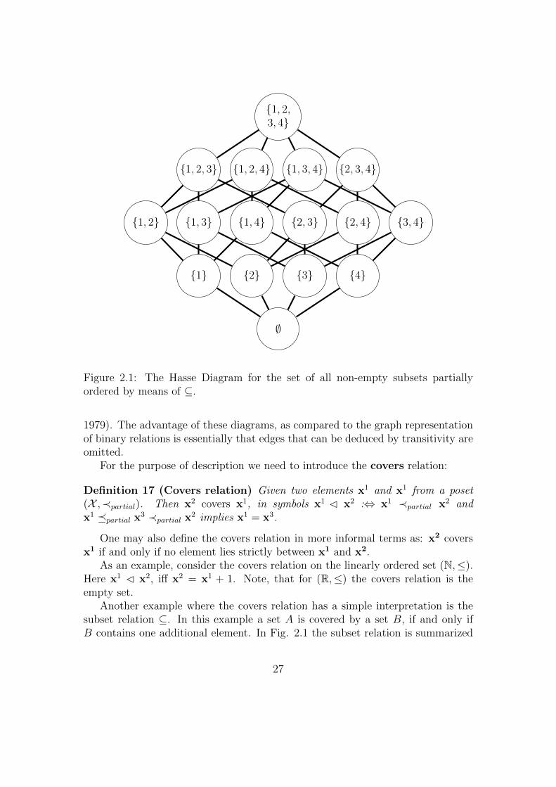
Figure 2.1: The Hasse Diagram for the set of all non-empty subsets partiallyordered by means of ⊆.

1979). The advantage of these diagrams, as compared to the graph representationof binary relations is essentially that edges that can be deduced by transitivity areomitted.

For the purpose of description we need to introduce the covers relation:

Definition 17 (Covers relation) Given two elements x1 and x1 from a poset(X ,≺partial). Then x2 covers x1, in symbols x1 C x2 :⇔ x1 ≺partial x2 andx1 partial x3 ≺partial x2 implies x1 = x3.

One may also define the covers relation in more informal terms as: x2 coversx1 if and only if no element lies strictly between x1 and x2.

As an example, consider the covers relation on the linearly ordered set (N,≤).Here x1 C x2, iff x2 = x1 + 1. Note, that for (R,≤) the covers relation is theempty set.

Another example where the covers relation has a simple interpretation is thesubset relation ⊆. In this example a set A is covered by a set B, if and only ifB contains one additional element. In Fig. 2.1 the subset relation is summarized

27

in a Hasse diagram. In this diagram the cover relation defines the arcs. A gooddescription of the algorithm to draw a Hasse diagram has been provided by Daveyand Priestly ([22], page 11):

Algorithm 1 Drawing the Hasse Diagram

1: To each point x ∈ S assign a point p(x), depicted by a small circle with centrep(x)

2: For each covering pair x1 and x2 draw a line segment `(x1,x2).3: Choose the center of circles in a way such that:4: whenever x1 C x2, then p(x1) is positioned below p(x2).5: if x3 6= x1 and x3 6= x2, then the circle of x3 does not intersect the line

segment `(x1,x2)

There are many ways of how to draw a Hasse diagram for a given order. Daveyand Priestly [22] note that diagram-drawing is ’as much an science as an art’.Good diagrams should provide an intuition for symmetries and regularities, andavoid crossing edges.

2.6 Comparing ordered sets

(Pre)ordered sets can be compared directly and on a structural level. Consider thefour orderings depicted in the Hasse diagrams of Fig. 2.2. It should be immediatelyclear, that the first two orders (1,2) on X have the same structure, but theyarrange elements in a different way, while orders 1 and 3 also differ in theirstructure. Moreover, it is evident that all comparisons defined in ≺1 are alsodefined in ≺3, but not vice versa (e.g. c and b are incomparable in 1). Theordered set on 3 is an extension of the ordered set 1. Another extension of 1

is given with 4.Let us now define these concepts formally:

Definition 18 (Order equality) An ordered set (X,) is said to be equal to anordered set (X,′), iff ∀x, y ∈ X : x y ⇔ x ′ y.

Definition 19 (Order isomorphism) An ordered set (X ′,≺′) is said to be anisomorphic to an ordered set (X,), iff there exists a mapping φ : X → X ′ suchthat ∀x, x′ ∈ X : x x′ ⇔ φ(x) ′ φ(x′). In case of two isomorphic orders, amapping φ is said to be an order embedding map or order isomorphism.

Definition 20 (Order extension) An ordered set (X,≺′) is said to be an ex-tension of an ordered set (X,≺), iff ∀x, x′ ∈ X : x ≺ x′ ⇒ x ≺′ x′. In the latter

28

case, ≺′ is said to be compatible with ≺. A linear extension is an extension thatis totally ordered.

Linear extensions play a vital role in the theory of multi-objective optimiza-tion. For Pareto orders on continuous vector spaces linear extensions can be easilyobtained by means of any weighted sum scalarization with positive weights. Ingeneral, topological sorting can serve as a means to obtain linear extensions. Bothtopics will be dealt with in more detail later in this work. For now, it should beclear that there can be many extensions of the same order, as in the example ofFig. 2.2, where (X,3) and (X,4) are both (linear) extensions of (X,1).

Apart from extensions, one may also ask if the structure of an ordered set iscontained as a substructure of another ordered set.

Definition 21 Given two ordered sets (X,) and (X ′,′). A map φ : X → X ′

is called order preserving, iff ∀x, x′ ∈ X : x x′ ⇒ φ(x) φ(x′).

Whenever (X,) is an extension of (X,′) the identity map serves as an orderpreserving map. An order embedding map is always order preserving, but not viceversa.

There is a rich theory on the topic of partial orders and it is still rapidlygrowing. Despite the simple axioms that define the structure of the poset, thereis a remarkably deep theory even on finite, partially ordered sets. The number ofordered sets that can be defined on a finite set with n members, denoted with sn,evolves as

sn∞1 = 1, 3, 19, 219, 4231, 130023, 6129859, 431723379, . . . (2.1)

and the number of equivalence classes, i.e. classes that contain only isomorphicstructures, denoted with Sn, evolves as:

Sn∞1 = 1, 2, 5, 16, 63, 318, 2045, 16999, ... (2.2)

. See Finch [34] for both of these results. This indicates how rapidly the structuralvariety of orders grows with increasing n. Up to now, no closed form expressionsfor the growth of the number of partial orders are known [34].

2.7 Cone orders

There is a large class of partial orders on Rm that can be defined geometrically bymeans of cones. In particular the so-called cone orders belong to this class. Coneorders satisfy two additional axioms. These are:

29

≤1

a

b

c

d

≤2

c

b

a

d

≤3

a

b

c

d

≤4

a

c

b

d

Figure 2.2: Different orders over the set X = a, b, c, d

Definition 22 (Translation invariance) Let R ∈ Rm × Rm denote a binaryrelation on Rm. Then R is translation invariant, if and only if for all t ∈ Rm,x1 ∈ Rm and x2 ∈ Rm: x1Rx2, if and only if (x1 + t)R(x2 + t).

Definition 23 (Multiplication invariance) Let R ∈ Rm×Rm denote a binaryrelation on Rm. Then R is multiplication invariant, if and only if for all α ∈ R,x1 ∈ Rm and x2 ∈ Rm: x1Rx2, if and only if (αx1)R(αx2).

We may also define these axioms on some other (vector) space on which translationand scalar multiplication is defined, but restrict ourselves to Rm as our interest ismainly to compare vectors of objective function values.

It has been found by V. Noghin [65] that the only partial orders on Rm thatsatisfy these two additional axioms are the cone orders on Rm defined by polyhedralcones. The Pareto dominance order is a special case of a strict cone order. Herethe definition of strictness is inherited from the pre-order.

Cone orders can be defined geometrically and doing so provides a good intuitionabout their properties and minimal sets.

Definition 24 (Cone) A subset C ⊆ Rm is called a cone, iff αd ∈ C for all d ∈ Cand for all α ∈ R, α > 0.

In order to deal with cones it is useful to introduce notations for set-basedcalculus by Minkowski:

Definition 25 (Minkowski sum) The Minkowski sum of two subsets S1 and S2

of Rm is defined as S1 +S2 := s1 + s2|s1 ∈ S1, s2 ∈ S2. If S1 is a singleton x,we may write s+ S2 instead of s+ S2.

30

Definition 26 (Minkowski product) The Minkowski product of a scalar α ∈Rn and a set S ⊂ Rn is defined as αS := αs|s ∈ S.

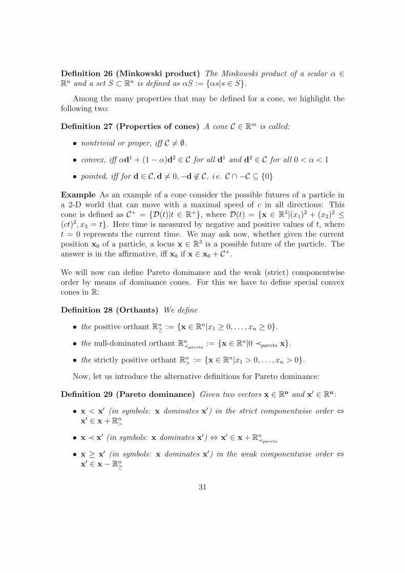
Among the many properties that may be defined for a cone, we highlight thefollowing two:

Definition 27 (Properties of cones) A cone C ∈ Rm is called:

• nontrivial or proper, iff C 6= ∅.

• convex, iff αd1 + (1− α)d2 ∈ C for all d1 and d2 ∈ C for all 0 < α < 1

• pointed, iff for d ∈ C,d 6= 0,−d 6∈ C, i e. C ∩ −C ⊆ 0

Example As an example of a cone consider the possible futures of a particle ina 2-D world that can move with a maximal speed of c in all directions: Thiscone is defined as C+ = D(t)|t ∈ R+, where D(t) = x ∈ R3|(x1)2 + (x2)

2 ≤(ct)2, x3 = t. Here time is measured by negative and positive values of t, wheret = 0 represents the current time. We may ask now, whether given the currentposition x0 of a particle, a locus x ∈ R3 is a possible future of the particle. Theanswer is in the affirmative, iff x0 if x ∈ x0 + C+.

We will now can define Pareto dominance and the weak (strict) componentwiseorder by means of dominance cones. For this we have to define special convexcones in R:

Definition 28 (Orthants) We define

• the positive orthant Rn≥ := x ∈ Rn|x1 ≥ 0, . . . , xn ≥ 0.

• the null-dominated orthant Rn≺pareto := x ∈ Rn|0 ≺pareto x.

• the strictly positive orthant Rn> := x ∈ Rn|x1 > 0, . . . , xn > 0.

Now, let us introduce the alternative definitions for Pareto dominance:

Definition 29 (Pareto dominance) Given two vectors x ∈ Rn and x′ ∈ Rn:

• x < x′ (in symbols: x dominates x′) in the strict componentwise order ⇔x′ ∈ x + Rn>

• x ≺ x′ (in symbols: x dominates x′) ⇔ x′ ∈ x + Rn≺pareto

• x ≥ x′ (in symbols: x dominates x′) in the weak componentwise order ⇔x′ ∈ x− Rn≥

31

Figure 2.3: Pareto domination in R2 defined by means of cones. In the left handside of the figure the points inside the dominated region are dominated by x. In thefigure on the right side the set of points dominated by the set A = x1,x2,x3,x4is depicted.

It is often easier to assess graphically whether a point dominates another pointby looking at cones (cf. Fig. 2.3 (l)). This holds also for a region that is dominatedby a set of points, such that at least one point from the set dominates it (cf. Fig.2.3 (r)).

Definition 30 (Dominance by a set of points) A point x is said to be domi-nated by a set of points A (notation: A ≺ x, iff x ∈ A + Rn≺, i. e. iff there existsa point x′ ∈ A, such that x′ ≺Pareto x.

In the theory of multiobjective and constrained optimization, so-called polyhe-dral cones play a crucial role.

Definition 31 A cone C is a polyhedral cone with a finite basis, if and only ifthere is a set of vectors D = d1, . . . ,dk ⊂ Rm and C = λ1d1 + · · · + λkdk|λ ∈R+

0 , i = 1, . . . , k.

By chosing the coordinate vectors ei to construct a polyhedral cones that resembleof the weak componentwise order.

Example In figure 2.4 an example of an cone is depicted with finite basis D =d1,d2 and d1 = (2, 1)>,d2 = (1, 2)>. It is defined as

C := λ1d1 + λ2d2|λ1 ∈ [0,∞], λ2 ∈ [0,∞] .

32

f1

f2

1

1

2

2

(0, 0)

Figure 2.4: Dominance cone for cone order in Example 2.7.

This cone is pointed, because C ∩−C = ∅. Moreover, C is a convex cone. This isbecause two points in C, say p1 and p2 can be expressed by p1 = λ11d1 + λ21d2

and p2 = λ12d1 + λ22d2, λij ∈ [0,∞), i = 1, 2; j = 1, 2. Now, for a given λ ∈ [0, 1]λp1+(1−λ)p2 equals λλ11d1+(1−λ)λ12d1 +λλ21d2+(1−λ)λ22d2 =: c1d1+c2d2,where it holds that c1 ∈ [0,∞) and c2 ∈ [0,∞). According to the definition of Cthe cone therefore the point λp1 + (1− λ)p2 is part of the cone C.

Further topics related to cone orders are addressed in [28].

Exercises

1. In definition 6 some common properties are defined that binary relationscan have and some examples are given below. Find further examples fromreal-life for binary relations! Which axioms from definition 6 do they obey!

2. Characterize incomparability (definition 10) axiomatically! What are theessential differences to indifference?

3. Describe the Pareto order on the set of 3-D hypercube edges (0, 1, 0)T ,(0, 0, 1)T , (1, 0, 0)T , (0, 0, 0)T , (0, 1, 1)T , (1, 0, 1), (1, 1, 0)T , (1, 1, 1)T by meansof the graph of a binary relation and by means of the Hasse diagram!

4. Prove, that (N − 1,) with a b ⇔ a mod b ≡ 0 is a partially orderedset. What are the minimal (maximal) elements of this set?

5. Prove that the time cone C+ is convex! Compare the Pareto order to theorder defined by time cones!

33

Chapter 3

Landscape Analysis

In this chapter we will come back to optimization problems, as defined in thefirst chapter. We will introduce different notions of Pareto optimality and discussnecessary and sufficient conditions for (Pareto) optimality and efficiency in theconstrained and unconstrained case. In many cases, optimality conditions directlypoint to solution methods for optimization problems. As in Pareto optimizationthere is rather a set of optimal solutions then a single optimal solution, we willalso look at possible structures of optimal sets.

3.1 Search Space vs. Objective Space

In Pareto optimization we are considering two spaces - the decision space or searchspace S and the objective space Y. The vector valued objective function f : S→ Yprovides the mapping from the decision space to the objective space. The set offeasible solutions X can be considered as a subset of the decision space, i. e. X ⊆ S.Given a set X of feasible solutions, we can define Y as the image of X under f .

The sets S and Y are usually not arbitrary sets. If we want to define optimiza-tion tasks, it is mandatory that an order structure is defined on Y. The space S isusually equipped with a neighborhood structure. This neighborhood structure isnot needed for defining global optima, but it is exploited, however, by optimizationalgorithms that gradually approach optima and in the formulation of local opti-mality conditions. Note, that the choice of neighborhood system may influencethe difficulty of an optimization problem significantly. Moreover, we note that thedefinition of neighborhood gives rise to many characterizations of functions, suchas local optimality and barriers. Especially in discrete spaces the neighborhoodstructure needs to be mentioned then, while in continuous optimization localitymostly refers to the Euclidean metric.

The definition of landscape is useful to distinguish the general concept of a

34

1111

1110 1101 1011 0111

1100 1010 1001 0110 0101 0011

1000 0100 0010 0001

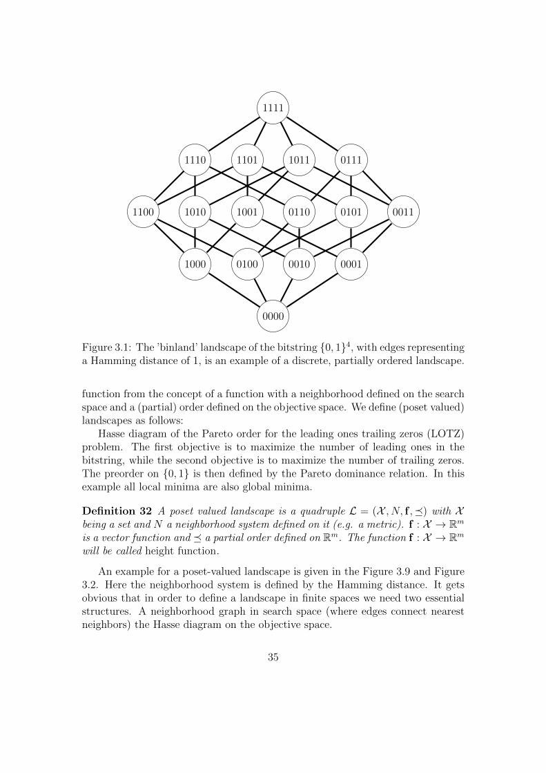
0000

Figure 3.1: The ’binland’ landscape of the bitstring 0, 14, with edges representinga Hamming distance of 1, is an example of a discrete, partially ordered landscape.

function from the concept of a function with a neighborhood defined on the searchspace and a (partial) order defined on the objective space. We define (poset valued)landscapes as follows:

Hasse diagram of the Pareto order for the leading ones trailing zeros (LOTZ)problem. The first objective is to maximize the number of leading ones in thebitstring, while the second objective is to maximize the number of trailing zeros.The preorder on 0, 1 is then defined by the Pareto dominance relation. In thisexample all local minima are also global minima.

Definition 32 A poset valued landscape is a quadruple L = (X , N, f ,) with Xbeing a set and N a neighborhood system defined on it (e.g. a metric). f : X → Rmis a vector function and a partial order defined on Rm. The function f : X → Rmwill be called height function.

An example for a poset-valued landscape is given in the Figure 3.9 and Figure3.2. Here the neighborhood system is defined by the Hamming distance. It getsobvious that in order to define a landscape in finite spaces we need two essentialstructures. A neighborhood graph in search space (where edges connect nearestneighbors) the Hasse diagram on the objective space.

35

0, 0 (0100, 0011, 0110, 0001, 0101, 0111)

1, 0 (1001, 1011) 0, 1 (0110, 0010)

1, 1 (1010)4, 0 (1111) 0, 4 (0000)

2, 2 (1100)3, 1 (1110) 1, 3 (1000)

Figure 3.2: (Figure 3.2) Hasse diagram of the Pareto order for the leading onestrailing zeros (LOTZ) problem. The first objective is to maximize the number ofleading ones in the bitstring, while the second objective is to maximize the numberof trailing zeros. The preorder on 0, 42 is then defined by the Pareto dominancerelation. In this example all local minima are also global minima (cf. Fig. 3.9).

Note, that for many definitions related to optimization we do not have to specifya height function and it suffices to define an order on the search space. For conceptslike global minima the neighborhood system is not relevant either. Therefore, thisdefinition should be understood as a kind of superset of the structure we may referto in multicriteria optimization.

3.2 Global Pareto Fronts and Efficient Sets

Given f : S → Rm. Here we write f instead of (f1, . . . , fm)>. Consider an opti-mization problem:

f(x)→ min,x ∈ X (3.1)

Recall that the Pareto front and the efficient set are defined as follows (Section1.5):

Definition 33 Pareto front and efficient setThe Pareto front YN is defined as the set of non-dominated solutions in Y =

f(X ), i. e. YN = y ∈ Y | @y′ ∈ Y : y′ ≺ y. The efficient set is defined as thepre-image of the Pareto-front, XE = f−1(YN).

Note, that the cardinality XE is at least as big as YN , but not vice versa,because there can be more than one point in XE with the same image in YN . Theelements of XE are termed efficient points.

In some cases it is more convenient to look at a direct definition of efficientpoints:

Definition 34 A point x(1) ∈ X is efficient, iff 6 ∃x(2) ∈ X : x(2) ≺ x(1).

36

x1

x2

1

1

2

2

(0, 0)f1

f2

1

1

2

2

(0, 0)

efficient

weakly efficient efficient

dominatedweakly

Figure 3.3: Example of a solution set containing efficient solutions (open points)and weakly efficient solutions (thick blue line).

Again, the set of all efficient solutions in X is denoted as XE.

Remark Efficiency is always relative to a set of solutions. In future, we will notalways consider this set to be the entire search space of an optimization problem,but we will also consider the efficient set of a subset of the search space. Forexample the efficient set for a finite sample of solutions from the search spacethat has been produced so far by an algorithm may be considered as a temporaryapproximation to the efficient set of the entire search space.

3.3 Weak efficiency

Besides the concept of efficiency also the concept of weak efficiency, for technicalreasons, is important in the field of multicriteria optimization. For example pointson the boundary of the dominated subspace are often characterized as weaklyefficient solutions though they may be not efficient.

Recall the definition of strict domination (Section 1.5):

Definition 35 Strict dominanceLet y(1),y(2) ∈ Rm denote two vectors in the objective space. Then y(1) strictly

dominates y(2) (in symbols: y(1) < y(2)), iff ∀i = 1, . . . ,m : y(1)i < y

(2)i .

Definition 36 Weakly efficient solutionA solution x(1) ∈ X is weakly efficient, iff 6 ∃x(2) ∈ X : f(x(2)) < f(x(1)). The

set of all weakly efficient solutions in X is called XwE.

37

f1

f2

y

N

y

minimum of f2

minimum of f1

Feasible objective space

Figure 3.4: The shaded region indicates the feasible objective space of some func-tion. Its ideal point, y, its Nadir point, N and its maximal point, y, are visible.

Example In Fig. 3.3 we graphically represent the efficient and weakly efficientset of the following problem: f = (f1, f2)→ min,S = X = [0, 2]× [0, 2], where f1and f2 are as follows:

f1(x1, x2) =

2 + x1 if 0 ≤ x2 < 11 + 0.5x1 otherwise

, f2(x1, x2) = 1+x1, x1 ∈ [0, 2], x2 ∈ [0, 2].

. The solutions (x1, x2) = (0, 0) and (x1, x2) = (0, 1) are efficient solutions ofthis problem, while the solutions on the line segments indicated by the bold linesegments in the figure denote weakly efficient solutions. Note, that both efficientsolutions are also weakly efficient, as efficiency implies weak efficiency.

3.4 Characteristics of Pareto Sets

There are some characteristic points on a Pareto front:

Definition 37 Given an multi-objective optimization problem with m objectivefunctions and image set Y: The ideal solution is defined as

y = (miny∈Y

y1, . . . ,miny∈Y

ym).

Accordingly we define the maximal solution:

y = (maxy∈Y

y1, . . . ,maxy∈Y

ym).

38

The Nadir point is defined:

yN = (maxy∈YN

y1, . . . , maxy∈YN

ym).

For the Nadir only points from the Pareto front YN are considered, while for themaximal point all points in Y are considered. The latter property makes it, fordimensions higher than two (m > 2), more difficult to compute the Nadir point.In that case the computation of the Nadir point cannot be reduced to m singlecriterion optimizations.

A visualization of these entities in a 2-D space is given in figure 3.4.

3.5 Optimality conditions based on level sets

Level sets can be used to visualize XE, XwE and XsE for continuous spaces andobtain these sets graphically in the low-dimensional case: Let in the followingdefinitions f be a function f : S→ R, for instance one of the objective functions:

Definition 38 Level sets

L≤(f(x)) = x ∈ X : f(x) ≤ f(x) (3.2)

Definition 39 Level curves

L=(f(x)) = x ∈ X : f(x) = f(x) (3.3)

Definition 40 Strict level set

L<(f(x)) = x ∈ X : f(x) < f(x) (3.4)

Level sets can be used to determine whether x ∈ X is (strictly, weakly) non-dominated or not.

The point x can only be efficient if its level sets intersect in level curves.

Theorem 41 x is efficient ⇔⋂mk=1 L≤(fk(x)) =

⋂mk=1 L=(fk(x))

Proof: x is efficient ⇔ there is no x such that both fk(x) ≤ fk(x) for all k =1, . . . ,m and fk(x) < f(x) for at least one k = 1, . . . ,m ⇔ there is no x ∈ X suchthat both x ∈ ∩mk=1L≤(f(x)) and x ∈ L<(fj(x)) for some j ⇔

⋂mk=1 L≤(fk(x)) =⋂m

k=1 L=(fk(x))

Theorem 42 The point x can only be weakly efficient if its strict level sets do notintersect. x is weakly efficient ⇔

⋂mk=1 L<(fk(x)) = ∅

39

x1

x2

1

1

2

2

(0, 0)

f1 = 1f1 = 4

f1 = 16

f2 = 0.25f2 = 1

f2 = 4

p1 p2

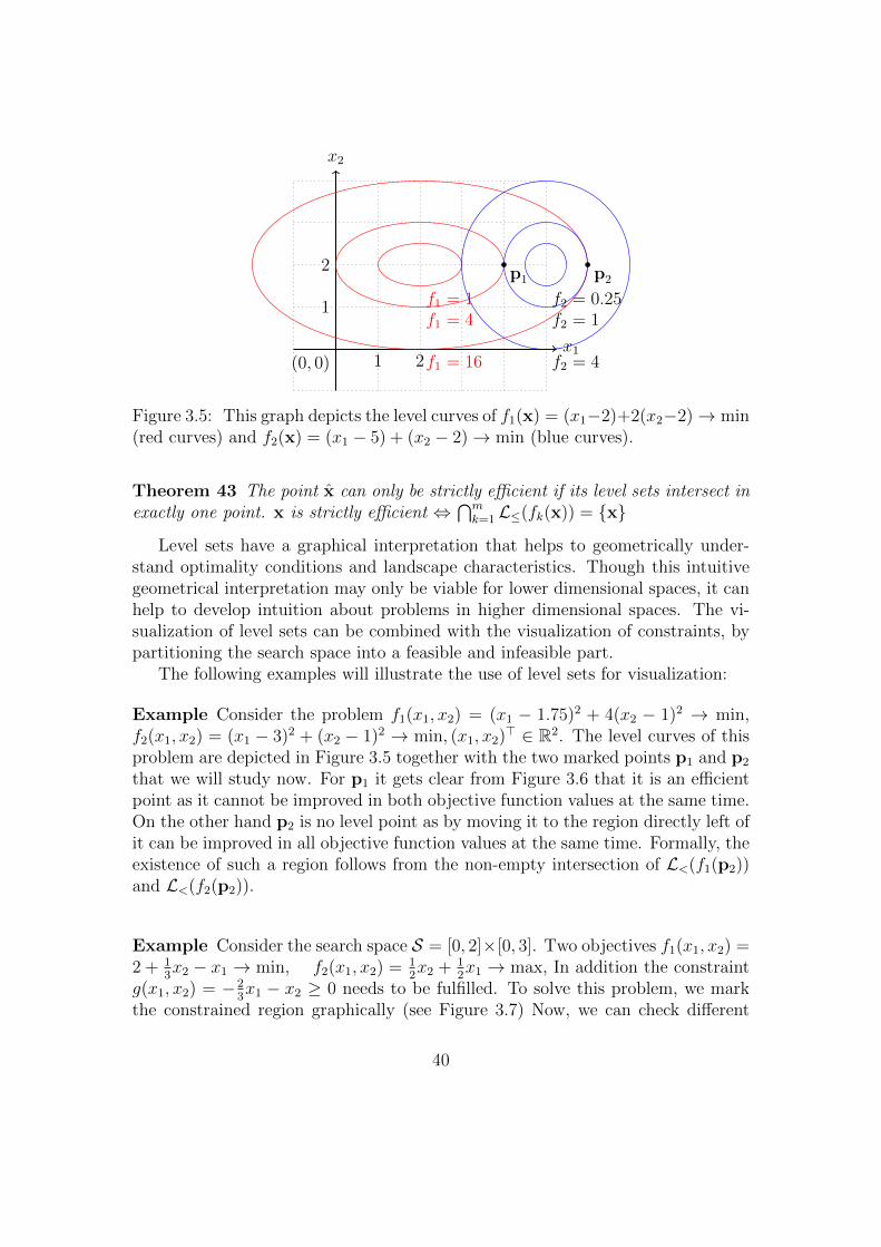
Figure 3.5: This graph depicts the level curves of f1(x) = (x1−2)+2(x2−2)→ min(red curves) and f2(x) = (x1 − 5) + (x2 − 2)→ min (blue curves).

Theorem 43 The point x can only be strictly efficient if its level sets intersect inexactly one point. x is strictly efficient ⇔

⋂mk=1 L≤(fk(x)) = x

Level sets have a graphical interpretation that helps to geometrically under-stand optimality conditions and landscape characteristics. Though this intuitivegeometrical interpretation may only be viable for lower dimensional spaces, it canhelp to develop intuition about problems in higher dimensional spaces. The vi-sualization of level sets can be combined with the visualization of constraints, bypartitioning the search space into a feasible and infeasible part.

The following examples will illustrate the use of level sets for visualization:

Example Consider the problem f1(x1, x2) = (x1 − 1.75)2 + 4(x2 − 1)2 → min,f2(x1, x2) = (x1 − 3)2 + (x2 − 1)2 → min, (x1, x2)

> ∈ R2. The level curves of thisproblem are depicted in Figure 3.5 together with the two marked points p1 and p2

that we will study now. For p1 it gets clear from Figure 3.6 that it is an efficientpoint as it cannot be improved in both objective function values at the same time.On the other hand p2 is no level point as by moving it to the region directly left ofit can be improved in all objective function values at the same time. Formally, theexistence of such a region follows from the non-empty intersection of L<(f1(p2))and L<(f2(p2)).

Example Consider the search space S = [0, 2]×[0, 3]. Two objectives f1(x1, x2) =2 + 1

3x2 − x1 → min, f2(x1, x2) = 1

2x2 + 1

2x1 → max, In addition the constraint

g(x1, x2) = −23x1 − x2 ≥ 0 needs to be fulfilled. To solve this problem, we mark

the constrained region graphically (see Figure 3.7) Now, we can check different

40

x1

x2

1

1

2

2

(0, 0)

L1

f1 = 1

L2

f2 = 1

p1

Figure 3.6: The situation for p1: In order to improve f1 the point p1 has tomove into the set L≤(f1(p1)) and in order to improve f2 it needs to move intoL≤(f1(p1)). Since these sets only meet in p1, it is not possible to improve f1 andf2 at the same time.

points for efficiency. For p1 the region where both objectives improve is in theupper triangle bounded by the level curves. As this set is partly feasible, it ispossible to find a dominating feasible point and p1 is not efficient. In contrast, forp2 the set of dominating solutions is completely in the infeasible domain, why thispoint belongs to the efficient set. The complete efficient set in this example lies onthe constraint boundary. Generally, it can be found that for linear problems withlevel curves intersecting in a single point there exists no efficient solutions in theunconstrained case whereas efficient solutions may lie on the constraint boundaryin the constrained case.

3.6 Local Pareto Optimality

As opposed to global Pareto optimality we may also define local Pareto optimality.Roughly speaking, a solution is a local optimum, if there is no better solution in itsneighborhood. In order to put things into more concrete terms let us distinguishcontinuous and discrete search spaces:

In finite discrete search spaces for each point in the search space X a set ofnearest neighbors can be defined by means of some neighborhood function N :X → ℘(X) with ∀x ∈ X : x 6∈ N(x). As an example consider the space 0, 1n ofbit-strings of length n with the nearest neigbors of a bit-string x being the elementsthat differ only in a single bit, i.e. that have a Hamming distance of 1.

41

0

x2

1

2

21 3

x1

f2=3

f2=1f2=2

f1=1

f1=2

p1

p2

Figure 3.7: Example for a linear programming problem visualization with twoobjective functions

Definition 44 Locally efficient point (finite search spaces)Given a neighborhood function N : X → ℘(X), a locally efficient solution is a

point x ∈ X such that 6 ∃x′ ∈ N(x) : x′ ≺ x.

Definition 45 Strictly locally efficient point (finite search spaces)Given a neighborhood function N : X → ℘(X), a strictly locally efficient solu-

tion is a point x ∈ X such that 6 ∃x′ ∈ N(x) : x′ x.

Remark: The comparison of two elements in the search space is done in theobjective space. Therefore, for two elements x and x′ with x x′ and x x′ itcan happen that x 6= x′ (see also the discussion of the antisymmetry property inchapter 2).

This definition can also be extended for countable infinite sets, though we mustbe cautious with the definition of the neighborhood function there.

For the Euclidean space Rn, the notion of nearest neighbors does not makesense, as for every point different from some point x there exists another pointdifferent from x that is closer to x. Here, the following criterion can be used toclassify local optima:

Definition 46 Open ε-ballAn open ε-ball Bε(x) around a point x ∈ Rn is defined as: Bε(x) = x′ ∈

X|d(x, x′) < ε.

42

f0 f4

f2 f6

f7f3

f1 f5

100

110

101

010

011 111

001

000

f0 f4

f2 f6

f7f3

f1 f5

100

110

101

010

011 111

001

000

Figure 3.8: Pseudoboolean landscapes with search space 0, 13 and the Hammingneighborhood defined on it. The linearly ordered landscape on the right hand sidehas three local optima. These are x(0) = 000, x(4) = 100, x(7) = 111. x(0) is also aglobal minimum and x(4) a global maximum. The partially ordered landscape onthe right hand side has locally efficient solutions are x(1) = 001, x(2) = 010, x(3) =011, x(6) = 110. The globally efficient solutions are x(1), x(2) and x(3)

Definition 47 Locally efficient point (Euclidean search spaces)A point x ∈ Rn in a metric space is said to be a locally efficient solution, iff

∃ε > 0 :6 ∃x′ ∈ Bε(x) : x′ ≺ x.

Definition 48 Strictly locally efficient point (Euclidean search spaces)A point x ∈ Rn in a metric space is said to be a strictly locally efficient solution,

iff ∃ε > 0 :6 ∃x′ ∈ Bε(x)− x : x′ x.

The extension of the concept of local optimality can be done also for subspacesof the Euclidean space, such as box constrained spaces as in definition 1.8.

3.7 Barrier Structures

Local optima are just one of the many characteristics we may discuss for land-scapes, i.e. functions with a neighborhood structure defined on the search space.Looking at different local optimal of a landscape we may ask ourselves how theselocal optimal are separated from each other. Surely there is some kind of barrier inbetween, i.e. in order to reach one local optimum from the other following a pathof neighbors in the search space we need to put up with encountering worseningof solutions along the path. We will next develop a formal framework on definingbarriers and their characteristics and highlight an interesting hierarchical structure

43

15 2 10 18 3

6 12 17 5 19

16 7 9 14 13

1 11 4 20 8

Figure 3.9: Example of a discrete landscape. The height of points is given by thenumbers and their neighborhood is expressed by the edges.

that can be obtained for all landscapes - the so called barrier tree of totally orderedlandscapes, which generalizes to a barrier forest in partially ordered landscapes.

For the sake of clarity let us introduce formal definitions first for landscapeswith a one-dimensional height function as they are discussed in single-objectiveoptimization.

Definition 49 Path in discrete spacesLet N : X→ ℘(X) be a neighborhood function. A sequence p1, . . . ,pl for some

l ∈ N and p1, . . . ,pl ∈ S is called a path connecting x1 and x2, iff p1 = x1,pi+1 ∈ N(pi), for i = 1, . . . , l − 1, and pl = x2.

Definition 50 Path in continuous spacesFor continuous spaces a path is a continuous mapping p[0, 1]→ X with p(0) =

x1 and p(1) = x2.

Definition 51 Let Px1,x2 denote the set of all paths between x1 and x2.

Definition 52 Let the function value of the lowest point separating two local min-ima x1 and x2 be defined as f(x1,x2) = minp∈Px1,x2 maxx3∈p f(x3). Points s on

some path p ∈ Px1,x2 for which f(s) = f(x1,x2) are called saddle points betweenx1 and x2.

Example In the example given in Figure 3.9 the search points are labeled by theirheights, i.e. x1 has height 1 and x4 has height 4. The saddle point between thelocal minima x1 and x2 is x12. The saddle point x3 and x5 is x18.

Lemma 53 For non-degenerate landscapes, i.e. landscapes where for all x1 andx2: f(x1) 6= f(x2), saddle points between two given local optima are unique.

44

Note. that in case of degenerate landscapes, i.e. landscapes where there are atleast two different points which share the same value of the height function, saddlepoints between two given local optima are not necessarily unique anymore, which,as we will see later, influences the uniqueness of barrier trees characterizing theoverall landscape.

Definition 54 The valley (or: basin) below a point s is called B(s) : B(s) = x ∈S|∃p ∈ Px,s : maxz∈p f(z) ≤ f(s)

Example In the aforementioned example given in Figure 3.9, Again, search pointsx1, . . . , x20 are labeled by their heights, i.e. x4 is the point with height 4, etc.. Thebasin below x1 is given by the empty set, and the basin below x14 is x1, x11, x4,x9, x7, x13, x5, x8, x14, x12, x2, x6, x10.

Points in B(s) are mutually connected by paths that never exceed f(s). At thispoint it is interesting to compare the level set L≤(f(x)) with the basin B(x). Theconnection between both concepts is: Let B be the set of connected components ofthe level set L≤(f(x)) with regard to the neighborhood graph of the search spaceX , then B(x) is the connected component in which x resides.

Theorem 55 Suppose for two points x1 and x2 that f(x1) ≤ f(x2). Then, eitherB(x1) ⊆ B(x2) or B(x1) ∩B(x2) = Ø.

Theorem 55 implies that the barrier structure of a landscapes can be repre-sented as a tree where the saddle points are the branching points and the localoptima are the leaves. The flooding algorithm (see Algorithm 2) can be used forthe construction of the barrier tree in discrete landscapes with finite search spaceX and linearly ordered search points (e.g. by means of the objective function val-ues). Note, that if the height function is not injective the flooding algorithm canstill be used but the barrier tree may not be uniquely defined. The reason for thisis that there are different possibilities of how to sort elements with equal heightsin line 1 of algorithm 2.

Finally, let us look whether concepts such as saddle points, basins, and barriertrees can be generalized in a meaningful way for partially ordered landscapes.Flamm and Stadler [76] recently proposed one way of generalizing these concepts.We will review their approach briefly and refer to the paper for details.

Adjacent points in linearly ordered landscapes are always comparable. Thisdoes not hold in general for partially ordered landscapes. We have to modify thepaths p that enter the definition.

Definition 56 Maximal points on a pathThe set of maximal points on a path p is defined as σ(p) = x ∈ p|@x′ ∈ p :f(x) ≺ f(x′)

45

Figure 3.10: A barrier tree of a 1-D continuous function.

Definition 57 Poset saddle-pointsΣx1,x2 =

⋃p∈Px1,x2

σ(p) is the set of maximal elements along all possible paths.

Poset-saddle points are defined as the Pareto optima1 of Σx1,x2: S(x1,x2) := z ∈Σx1,x2|@u ∈ Σx1,x2 : f(u) ≺ f(z)

The flooding algorithm can be modified in a way that incomparable elementsare not considered as neighbors (’moves to incomparable solutions are disallowed’).The flooding algorithm may then lead to a forest instead of a tree. For examples(multicriteria knapsack problem, RNA folding) and further discussion of how toefficiently implement this algorithm the reader is referred to [76].

A barrier tree for a continuous landscape is drawn in Fig. 3.10. In this case thesaddle points correspond to local maxima. For continuous landscapes the conceptof barrier trees can be generalized, but the implementation of flooding algorithmsis more challenging due to the infinite number of points that need to be considered.Discretization could be used to get a rough impression of the landscape’s geometry.

3.8 Shapes of Pareto Fronts

An interesting, since very general, questions could be: How can the geometricalshapes of Pareto fronts be classified. We will first look at some general descrip-tions used in literature on how to define the Pareto front w.r.t. convexity andconnectedness. To state definitions in an unambiguous way we will make use ofMinkowski sums and cones as defined in chapter 2.

1here we think of minimization of the objectives.

46

Algorithm 2 Flooding algorithm

1: Let x(1), . . . , x(N) denote the elements of the search space sorted in ascendingorder.

2: i→ 1;B = ∅3: while i ≤ N do4: if N(xi) ∩ x(1), . . . , x(i−1) = ∅ [i. e., x(i) has no neighbour that has been

processed.] then5: x(i) is local minimum6: Draw x(i) as a new leaf representing basin B(x(i)) located at the height

of f in the 2-D diagram7: B ← B ∪ B(x(i)) Update set of basins8: else9: Let T (x(i)) = B(x(i1)), . . . , B(x(iN )) be the set of basins B ∈ B with

N(x(i)) ∩B 6= ∅.10: if |T (x(i))| = 1 then11: B(x(i1))← B(x(i1)) ∪ x(i)12: else13: x(i) is a saddle point14: Draw x(i) as a new branching point connecting the nodes for

B(x(i1)), . . . , B(x(iN )). Annotate saddle point node with B(x(i)) andlocate it at the height of f in the 2-D diagram

15: Update set of basins16: B(x(i)) = B(x(i1)) ∪ · · · ∪B(x(iN )) ∪ x(i)17: Remove B(x(i1)), . . . , B(x(iN )) from B18: B ← B ∪ B(x(i))19: end if20: end if21: end while

47

Figure 3.11: Different shapes of Pareto fronts for bi-criteria problems.

Definition 58 A set Y ⊆ Rm is said to be cone convex w.r.t. the positive orthant,iff YN + Rm≥ is a convex set.

Definition 59 A set Y ⊆ Rm is said to be cone concave w.r.t. the positive orthant,iff YN − Rm≥ is a convex set.

Definition 60 A Pareto front YN is said to be convex (concave), iff it is coneconvex (concave) w.r.t. the positive orthant.

Note, that Pareto fronts can be convex, concave, or may consist of cone convexand cone concave parts w.r.t. the positive orthant.

Convex Pareto fronts allow for better compromise solutions than concave Paretofronts. In the ideal case of a convex Pareto front, the Pareto front consists onlyon a single point which is optimal for all objectives. In this situation the deci-sion maker can choose a solution that satisfies all objectives at the same time.The most difficult situation for the decision maker arises, when the Pareto frontconsists of a separate set of points, one point for each single objective, and thesepoints are separate and very distant from each other. In such a case the decisionmaker needs to make a either-or decision.

Another classifying criterion of Pareto fronts is connectedness.

48

Definition 61 A Pareto front YN is said to be connected, if and only if for ally1,y2 ∈ YN there exists a continuous mapping φ : [0, 1]→ YN with φ(0) = y1 andφ(1) = y2.

For the frequently occurring case of two objectives, examples of convex, con-cave, connected and disconnected Pareto fronts are given in Fig. 3.11.

Two further corollaries highlight general characteristics of Pareto-fronts:

Lemma 62 Dimension of the Pareto frontPareto fronts for problems with m-objectives are subsets or equal to m − 1-

dimensional manifolds.

Lemma 63 Functional dependencies in the Pareto frontLet YN denote a Pareto front for some multiobjective problem. Then for any

sub-vector in the projection to the coordinates in 1, . . . ,m without i, the valueof the i-th coordinate is uniquely determined.

Example For a problem with three objectives the Pareto front is a subset of a2-D manifold that can be represented as a function from the values of the

• first two objectives to the third objective.

• the first and third objective to the second objective

• the last two objectives to the first objective

3.9 Conclusions

In this chapter the focus was on the different types of landscapes, shapes of optimain multiobjective optimization. A general technique to visualize and analyse mul-ticriteria landscapes based on level sets was provided, which also provides insightsinto the solution of linear programming problems. Moreover, with emphasize ondiscrete landscapes, the structure of multicriteria landscapes was discussed. Herethe barrier tree can be used to figure out, how landscapes are decomposed into val-leys and hills and how these are separated from each other. Finally, a classificationof different shapes of Pareto fronts was discussed and some general characteristicsof such sets were highlighted.

So far, the definitions we used did not exploit differentiability. If differentiabil-ity is provided the search for Pareto optima can be supported by powerful theoremsas will be discussed in the following chapter.

49

Chapter 4

Optimality conditions fordifferentiable problems

In the finite discrete case local optimality of a point x ∈ X can be done by com-paring it to all neighboring solutions. In the continuous case this is not possible,For differentiable problems we can state conditions for local optimality. We willstart with looking at unconstrained optimization, then provide conditions for opti-mization with equality and inequality constraints and, thereafter, their extensionsfor the multiobjective case.

4.1 Linear approximations

A general observation we should keep in mind when understanding optimizationconditions for differentiable problems is that continuously differentiable functionsf : Rn → R can be locally approximated at any point x(0) by means of linearapproximations f(x(0)) + ∇f(x(0))(x − x0) with ∇f = ( ∂f

∂x1, . . . , ∂f

∂xn)>. In other

words:limx→x0

f(x)− [f(x0) +∇f(x)(x− x0)] = 0 (4.1)

The gradient ∇f(x(0)) points in the direction of steepest ascent and is orthog-onal to the level curves L=(f(x)) at the point x. This has been visualized in Fig.4.1.

4.2 Unconstrained Optimization

For the unconstrained minimization

f(x)→ min (4.2)

50

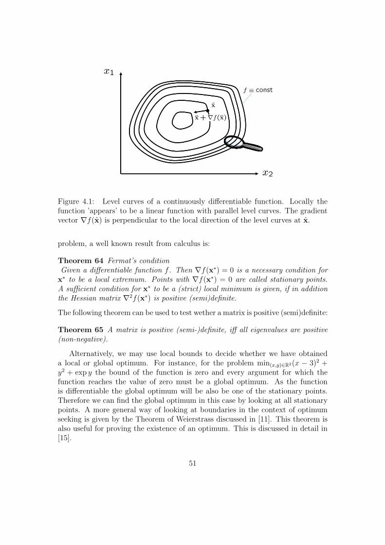
Figure 4.1: Level curves of a continuously differentiable function. Locally thefunction ’appears’ to be a linear function with parallel level curves. The gradientvector ∇f(x) is perpendicular to the local direction of the level curves at x.

problem, a well known result from calculus is:

Theorem 64 Fermat’s conditionGiven a differentiable function f . Then ∇f(x∗) = 0 is a necessary condition for

x∗ to be a local extremum. Points with ∇f(x∗) = 0 are called stationary points.A sufficient condition for x∗ to be a (strict) local minimum is given, if in additionthe Hessian matrix ∇2f(x∗) is positive (semi)definite.

The following theorem can be used to test wether a matrix is positive (semi)definite:

Theorem 65 A matrix is positive (semi-)definite, iff all eigenvalues are positive(non-negative).

Alternatively, we may use local bounds to decide whether we have obtaineda local or global optimum. For instance, for the problem min(x,y)∈R2(x − 3)2 +y2 + exp y the bound of the function is zero and every argument for which thefunction reaches the value of zero must be a global optimum. As the functionis differentiable the global optimum will be also be one of the stationary points.Therefore we can find the global optimum in this case by looking at all stationarypoints. A more general way of looking at boundaries in the context of optimumseeking is given by the Theorem of Weierstrass discussed in [11]. This theorem isalso useful for proving the existence of an optimum. This is discussed in detail in[15].

51

Theorem 66 Theorem of WeierstrassLet X be some closed1 and bounded subset of Rn, let f : X → R denote a continuousfunction. Then f attains a global maximum and minimum in X , i. e. ∃xmin ∈ X :∀x′ ∈ X : f(xmin) ≤ f(x′) and ∃xmax ∈ X : ∀x′ ∈ X : f(xmax) ≥ f(x′).

4.3 Equality Constraints

By introducing Lagrange multipliers, theorem 64 can be extended to problemswith equality constraints, i. e.:

f(x)→ min, s.t. g1(x) = 0, . . . , gm(x) = 0 (4.3)

In this case the following theorem holds:

Theorem 67 Let f and g1, . . . , gm denote differentiable functions. Then a nec-essary condition for x∗ to be a local extremum is given, if there exist multipliersλ1, . . . , λm+1 with at least one λi 6= 0 for i = 1, . . . ,m such that λ1∇f(x∗) +∑m+1

i=2 λi∇g(x∗) = 0.

For a rigorous proof of this theorem we refer to [15]. Let us remark, that thediscovery of this theorem by Lagrange preceded its proof by one hundred years[15].

Next, by means of an example we will provide some geometric intuition for thistheorem. In Fig. 4.2 a problem with a search space of dimension two is given. Asingle objective function f has to be maximized, and the sole constraint functiong1(x) is set to 0.

Let us first look at the level curve f ≡ −13. This curve does not intersectwith the level curve g ≡ 0 and thus there is no feasible solution on this curve.Next, we look at f ≡ −15. In this case the two curve intersects in two points withg ≡ 0. However, these solutions are not optimal. We can do better by moving tothe point, where the level curve of f ≡ c ’just’ intersects with g ≡ 0. This is thetangent point x∗ with c = f(x∗) = −14.

The tangential point satisfies the condition that the gradient vectors are collinearto each other, i.e. ∃λ 6= 0 : λ∇g(x∗) = ∇f(x∗). In other words, the tangent lineto the f level curve at a touching point is equal to the tangent line to the g ≡ 0level curve. Equality of tangent lines is equivalent to the fact that the gradientvectors are collinear.

Another way to reason about the location of optima is to check for each pointon the constraint curve whether it can be locally improved or not. For points wherethe level curve of the objective function intersects with the constraint function, we

1Roughly speaking, a closed set is a set which includes all points at its boundary.

52

Figure 4.2: Lagrange multipliers: Level-sets for a single objective and single activeconstraint and search space R2.

consider the local linear approximation of the objective function. In case of non-zero gradients, we can always improve the point further. In case of zero gradientswe already fulfill conditions of the theorem by setting λ1 = 1 and λi = 0 fori = 2, . . . ,m+ 1. This way we can exclude all points but the tangential points andlocal minima of the objective function (unconstrained) from consideration.

In practical optimization often λ1 is set to 1. Then the equations in the lagrangemultiplier theorem boil down to an equation system with m + n unknowns andm+n equations and this gives rise to a set of candidate solutions for the problem.This way of solving an optimization problem is called the Lagrange multiplier rule.

Example Consider the following problem:

f(x1, x2) = x21 + x22 → min (4.4)

, with equality constraint

g(x1, x2) = x1 + x2 − 1 = 0 (4.5)

Due to the theorem of 67, iff (x1, x2)> is a local optimum, then there exist λ1 and

λ2 with (λ1, λ2) 6= (0, 0) such that the constraint in equation 4.5 is fulfilled and

λ1∂f

∂x1+ λ2

∂g

∂x1= 2λ1x1 + λ2 = 0 (4.6)

53

λ1∂f

∂x2+ λ2

∂g

∂x2= 2λ1x2 + λ2 = 0 (4.7)

Let us first examine the case λ1 = 0. This entails:

λ2 = 0 (4.8)

This contradicts the condition that (λ1, λ2) 6= (0, 0).We did not yet prove, that the solution we found is also a global optimum. In

order to do so we can invoke Weierstrass theorem, by first reducing the problemto a problem with a reduced search space, say:

f|A → min (4.9)

A = (x1, x2)||x1| ≤ 10 and |x2| ≤ 10 and x1 + x2 − 1 = 0 (4.10)

For this problem a global minimum exists, due to the Weierstrass theorem(the set A is bounded and closed and f is continuous). Therefore, the originalproblem also has a global minimum in A, as for points outside A the functionvalue is bigger than 199 and in A there are points x ∈ A where f(x1, x2) < 199.The (necessary) Lagrange conditions, however, are only satisfied for one point inR2 which consequently must be the only local minimum and thus it is the globalminimum.

Now we consider the case λ1 = 1. This leads to the conditions:

2x1 + λ2 = 0 (4.11)

2x2 + λ2 = 0 (4.12)

and hence x1 = x2. From the equality condition we get: From the constraint itfollows x1 + x1 = 1, which entails x1 = x2 = 1

2.

Another possibility to solve this problem is by means of substitution: x1 =1−x2 and the objective function can then be written as f(1−x2, x2) = (1−x2)2+x22.Now minimize the unconstrained ’substitute’ function h(x2) = (1 − x2)

2 + x22.∂hx2

= −2(1 − x2) + 2x2 = 0. This yields x2 = 12. The second derivative ∂2f

∂2x2= 4.

This means that the point is a local minimum.

However, not always all candidate solutions for local optima are captured this wayas the case λ1 = 0 may well be relevant. Brinkhuis and Tikhomirov [15] give anexample of such a ’bad’ case:

Example Apply the multiplier rule to f0(x) → min, x21 − x32 = 0: The Lagrangeequations hold at x with λ0 = 0 and λ1 = 1. An interesting observation is thatthe level curves are cusp in this case at x, as visualized in Fig. 4.3.

54

Figure 4.3: The level curves of x21 − x32. The level curve through (0, 0)T is cusp.

4.4 Inequality Constraints

For inequality constraints the Karush Kuhn Tucker conditions are used as opti-mality criterion:

Theorem 68 The Karush Kuhn Tucker conditions are said to hold for x∗, if thereexist multipliers λ1 ≥ 0, . . . , λm+1 ≥ 0 and at least one λi > 0 for i = 1, . . . ,m+1,such that:

λ1∇f(x∗) +m∑i=1

λi+1∇gi(x∗) = 0 (4.13)

λi+1gi(x∗) = 0, i = 1, . . . ,m (4.14)

Theorem 69 Karush Kuhn Tucker Theorem (Necessary conditions for smooth,convex programming:)Assume the objective and all constraint functions are convex in some ε-neighborhoodof x∗, If x∗ is a local minimum, then there exiss λ1, . . . , λm+1 such that KKT con-ditions are fulfilled.

Theorem 70 The KKT conditions are sufficient for optimiality, provided λ1 = 1.In this case x∗ is a local minimum.

Note that if x∗ is in the interior of the feasible region (a Slater point), allgi(x) < 0 and thus λ1 > 0.

The next examples discuss the usage of the Karush Kuhn conditions:

55

Example In order to get familiar with the KKT theorem we apply it to a verysimple situation (solvable also with high school mathematics). The task is:

1− x2 → min, x ∈ [−1, 3]2 (4.15)

First, write the task in its standard form:

f(x) = 1− x2 → min (4.16)

subject to constraintsg1(x) = −x− 1 ≤ 0 (4.17)

g2(x) = x− 3 ≤ 0 (4.18)

The existence of the optimum follows from Weierstrass theorem, as (1) thefeasible subspace [-1,3] is bounded and closed and (2) the objective function iscontinuous.

The KKT conditions in this case boil down to: There exists λ1 ∈ R, λ2 ∈ R+0

and λ3 ∈ R+0 and (λ1, λ2, λ3) 6= (0, 0, 0) such that

λ1∂f

∂x+ λ2

∂g1∂x

+ λ3∂g1∂x

= −2λ1x− λ2 + λ3 = 0 (4.19)

λ2(−x− 1) = 0 (4.20)

λ3(x− 3) = 0 (4.21)

.First, let us check whether λ1 = 0 can occur:In this case the three equations (4.19, 4.20, and 4.21) will be:

−λ2 + λ3 = 0 (4.22)

λ2(−x− 1) = 0 (4.23)

λ3(x− 3) = 0 (4.24)

.and (λ2, λ3) 6= (0, 0), and λi ≥ 0, i = 2, 3. From 4.22 we see that λ2 = λ3. By

setting λ = λ2 we can writeλ(−x− 1) = 0 (4.25)

andλ(x− 3) = 0 (4.26)

for the equations 4.23 and 4.24. Moreover λ 6= 0, for (λ, λ) = (λ2, λ3) 6= (0, 0).From this we get that −x− 1 = 0 and x− 3 = 0. Which is a contradiction so thecase λ1 = 0 cannot occur – later we shall see that this could have derived by using

56

a theorem on Slater points 70.Next we consider the case λ1 6= 0 (or equivalently λ1 = 1): In this case the threeequations (4.19, 4.20, and 4.21) will be:

−2x− λ2 + λ3 = 0 (4.27)

,λ2(−x− 1) = 0 (4.28)

, andλ3(x− 3) = 0 (4.29)

We consider four subcases:

case 1: λ2 = λ3 = 0. This gives rise to x = 0

case 2: λ2 = 0 and λ3 6= 0. In this case we get as a condition on x: 2x(x− 3) = 0and x 6= 0 or equivalently x = 3

case 3: λ2 6= 0 and λ3 = 0. We get from this: −2x(−x − 1) = 0 and x 6= 0 orequivalently x = −1.

case 4: λ2 6= 0 and λ3 6= 0. This cannot occur as this gives rise to −x − 1 = 0and x− 3 = 0 (contradictory conditions).

In summary we see that a maximum can possibly only occur in x = −1, x = 0or x = 3. By evaluating f on these three candidates, we see that f attains itsglobal minimum in x = 3 and the value of the global minimum is −8. Note thatwe invoked also the Weierstrass theorem in the last conclusion: the Weierstrasstheorem tells us that the function f has a global minimum in the feasible region([-1.3]) and KKT (necessary conditions) tell us that it must be one of the threeabove mentioned candidates.

4.5 Multiple Objectives

For a recent generalization of the Lagrange multiplier rule to multiobjective opti-mization we refer to [38]. For multicriterion optimisation the KKT conditions canbe generalized as follows:

Theorem 71 Fritz John necessary conditionsA neccessary condition for x∗ to be a locally efficient point is that there exist vectorsλ1, . . . , λk and υ1, . . . , υm such that

λ 0, υ 0 (4.30)

57

Figure 4.4: Level curves of the two objectives touching in one point indicatelocally Pareto optimal points in the bi-criterion case, provided the functions aredifferentiable.

k∑i=1

λi∇fi(x∗)−m∑i=1

υi∇gi(x∗) = 0. (4.31)

υigi(x∗) = 0, i = 1, . . . ,m (4.32)

A sufficient condition for points to be Pareto optima follows:

Theorem 72 Karush Kuhn Tucker sufficient conditions for a solution to be Paretooptimal:Let x∗ be a feasible point. Assume that all objective functions are locally convexand all constraint functions are locally concave, and the Fritz John conditions holdin x∗, then x∗ is a local efficient point.

In the unconstrained case we get the simple condition:

Corollary 73 In the unconstrained case Fritz John neccessary conditions reduceto

λ 0 (4.33)

k∑i=1

λi∇fi(x∗) = 0. (4.34)

In 2-dimensional spaces this criterion reduces to the observation, that either oneof the objectives has a zero gradient (neccesary condition for ideal points) or thegradients are collinear as depicted in Fig. 4.4. A detailed description of theconditions for multiobjective optimization is given in [62].

58

Chapter 5

Scalarization Methods

A straightforward idea to recast a multiobjective problem as a single objectiveproblem is to sum up the objectives in an weighted sum and then to maxi-mize/minimize the weighted sum of objectives. More general is the approachto aggregate the objectives to a single objective by a so-called utility function,which does not have to be a linear sum but usually meets certain monotonicitycriteria. Techniques that sum up multiple objectives into a single one by mean ofan aggregate function are termed scalarization techniques. A couple of questionsarise when applying such techniques:

• Does the global optimization of the aggregate function always (or in certaincases) result in an efficient point?

• Can all solutions on the Pareto front be obtained by varying the (weight)parameters of the aggregate function?

• Given that the optimization of the aggregate leads to an efficient point, howdoes the choice of the weights control the position of the obtained solutionon the Pareto front?

Section 5.1 starts with linear aggregation (weighted sum) and answers theaforementioned questions for it. The insights we gain from the linear case prepareus for the generalization to nonlinear aggregation in Section 5.2. The expressionor modeling of preferences by means of of aggregate functions is a broad field ofstudy called Multi-attribute utility theory (MAUT). An overview and examplesare given in Section 5.3. A common approach to solve multicriteria optimizationproblems is the distance to a reference point method. Here the decision pointerdefines an desired ’utopia’ point and minimizes the distance to it. In Section 5.4we will discuss this method as a special case of a scalarization technique.

59

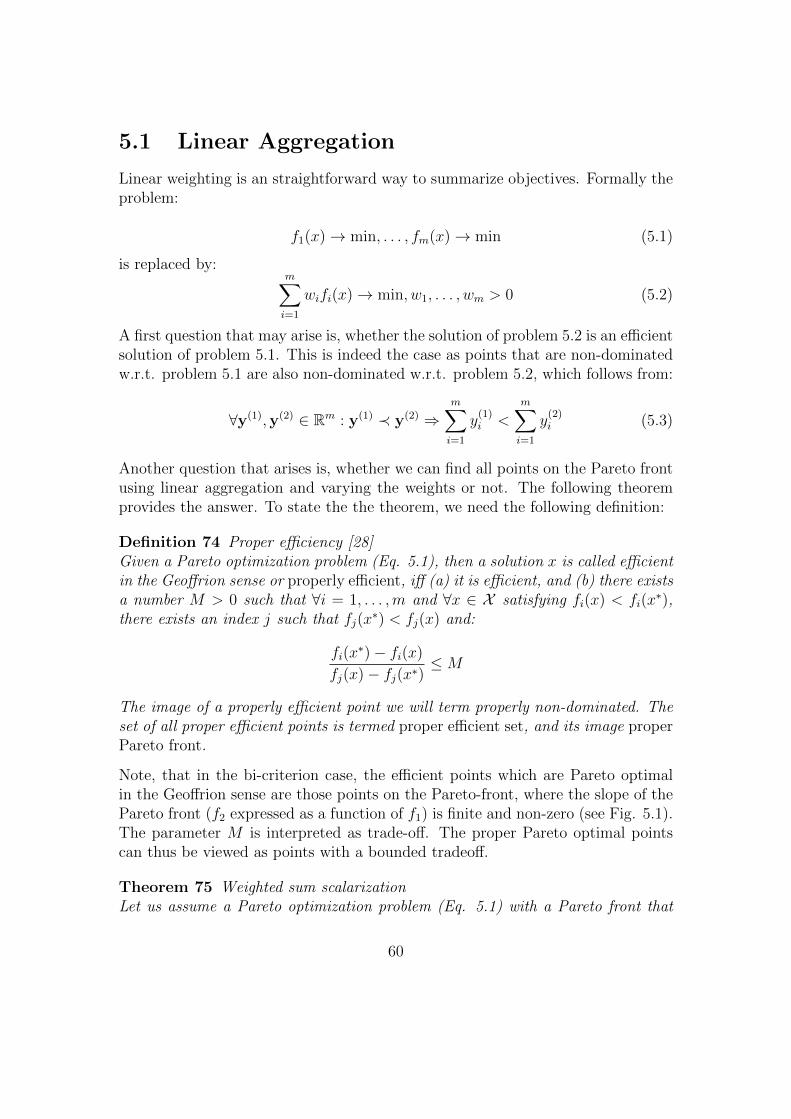
5.1 Linear Aggregation

Linear weighting is an straightforward way to summarize objectives. Formally theproblem:

f1(x)→ min, . . . , fm(x)→ min (5.1)

is replaced by:m∑i=1

wifi(x)→ min, w1, . . . , wm > 0 (5.2)

A first question that may arise is, whether the solution of problem 5.2 is an efficientsolution of problem 5.1. This is indeed the case as points that are non-dominatedw.r.t. problem 5.1 are also non-dominated w.r.t. problem 5.2, which follows from:

∀y(1),y(2) ∈ Rm : y(1) ≺ y(2) ⇒m∑i=1

y(1)i <

m∑i=1

y(2)i (5.3)

Another question that arises is, whether we can find all points on the Pareto frontusing linear aggregation and varying the weights or not. The following theoremprovides the answer. To state the the theorem, we need the following definition:

Definition 74 Proper efficiency [28]Given a Pareto optimization problem (Eq. 5.1), then a solution x is called efficientin the Geoffrion sense or properly efficient, iff (a) it is efficient, and (b) there existsa number M > 0 such that ∀i = 1, . . . ,m and ∀x ∈ X satisfying fi(x) < fi(x

∗),there exists an index j such that fj(x

∗) < fj(x) and:

fi(x∗)− fi(x)

fj(x)− fj(x∗)≤M

The image of a properly efficient point we will term properly non-dominated. Theset of all proper efficient points is termed proper efficient set, and its image properPareto front.

Note, that in the bi-criterion case, the efficient points which are Pareto optimalin the Geoffrion sense are those points on the Pareto-front, where the slope of thePareto front (f2 expressed as a function of f1) is finite and non-zero (see Fig. 5.1).The parameter M is interpreted as trade-off. The proper Pareto optimal pointscan thus be viewed as points with a bounded tradeoff.

Theorem 75 Weighted sum scalarizationLet us assume a Pareto optimization problem (Eq. 5.1) with a Pareto front that

60

Figure 5.1: The proper Pareto front for a bicriteria problem, for which in additionto many proper Pareto optimal solutions there exist also two non-proper Paretooptimal solutions.

is cone convex w.r.t. positive orthant (Rm≥). Then for each properly efficient pointx ∈ X there exist weights w1 > 0, . . . , wm > 0 such that x is one of the solutionsof∑m

i=1 fi(x)→ min.

In case of problems with a non-convex pareto front it is not always possible tofind weights for a given proper efficient point x such that x is one of the solutionsof∑m

i=1 fi(x)→ min. A counterexample is given in the following example:

Example In Fig. 5.2 the Pareto fronts of two different bi-criterion problems areshown. The figure on the right hand side shows a Pareto front which is cone convexwith respect to the positive orthant. Here the tangential points of the level curvesof w1y1 + w2y2 are the solutions obtained with linear aggregation. Obviously, bychanging the slope of the level curves by varying one (or both) of the weights, allpoints on the Pareto front can be obtained (and no other). On the other hand, forthe concave Pareto front shown on the right hand side only the extreme solutionsat the boundary can be obtained.

As the example shows linear aggregation has a tendency to obtain extremesolutions on the Pareto front, and its use is thus problematic in cases where noa-priori knowledge of the shape of the Pareto front is given. However, there existaggregation functions which have less tendency to obtain extreme solutions or evenallow to obtain all Pareto optimal solutions. They will be discussed in the nextsection.

61

Figure 5.2: The concave (left) and convex Pareto front (right).

5.2 Nonlinear Aggregation

Instead of linear aggregation we can use nonlinear aggregation approaches, e.g.compute a product of the objective function value. The theory of utility functionscan be viewed as a modeling approach for (non)linear aggregation functions.

A utility function assigns to each combination of values that may occur in theobjective space a scalar value - the so-called utility. This value is to be maximized.Note that the linear aggregation was to be minimized. Level curves of the utilityfunction are interpreted as indifference curves (see Fig. 5.3).

In order to discuss a scalarization method it may be interesting to analyze whereon the Pareto front the Pareto optimal solution that is found by maximizing theutility function is located. Similar to the linear weighting function discussed earlier,this is the point where the level curves of the utility (looked upon in descendingorder) first intersect with the Pareto front (see Fig. 5.4).

5.3 Multi-Attribute Utility Theory

Next, we will discuss a concrete example for the design of a utility function. Thisexample will illustrate many aspects of how to construct utility functions in apractically useful, consistent, and user-friendly way.

Example Consider you want to buy a car. Then you may focus on three objec-tives: speed, price, fuel-consumption. These three criteria can be weighted. It isoften not wise to measure the contribution of an objective function to the over-all utility in a linear way. A elegant way to model it is by specifying a functionthat measures the degree of satisfaction. For each possible value of the objective

62

Figure 5.3: Utility function for a bi-criterion problem. If the decision-maker hasmodeled this utility function in a proper way, he/she will be indifferent whetherto choose y(2) and y(3), but prefer y(3) and y(2) to y(1).

Figure 5.4: The tangential point of the Pareto front with the indifference curvesof the utility function U here determines where the solution of the maximizationof the utility function lies on the Pareto front.

63

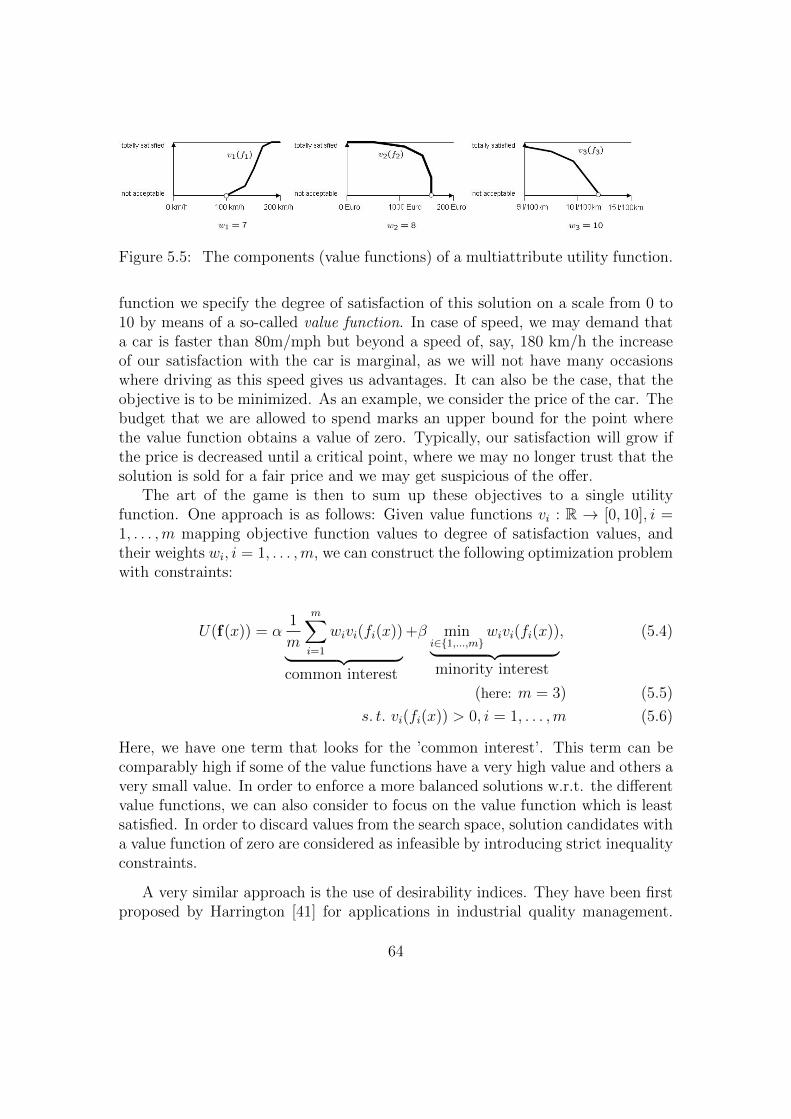
Figure 5.5: The components (value functions) of a multiattribute utility function.

function we specify the degree of satisfaction of this solution on a scale from 0 to10 by means of a so-called value function. In case of speed, we may demand thata car is faster than 80m/mph but beyond a speed of, say, 180 km/h the increaseof our satisfaction with the car is marginal, as we will not have many occasionswhere driving as this speed gives us advantages. It can also be the case, that theobjective is to be minimized. As an example, we consider the price of the car. Thebudget that we are allowed to spend marks an upper bound for the point wherethe value function obtains a value of zero. Typically, our satisfaction will grow ifthe price is decreased until a critical point, where we may no longer trust that thesolution is sold for a fair price and we may get suspicious of the offer.

The art of the game is then to sum up these objectives to a single utilityfunction. One approach is as follows: Given value functions vi : R → [0, 10], i =1, . . . ,m mapping objective function values to degree of satisfaction values, andtheir weights wi, i = 1, . . . ,m, we can construct the following optimization problemwith constraints:

U(f(x)) = α1

m

m∑i=1

wivi(fi(x))︸ ︷︷ ︸common interest

+β mini∈1,...,m

wivi(fi(x))︸ ︷︷ ︸minority interest

, (5.4)

(here: m = 3) (5.5)

s. t. vi(fi(x)) > 0, i = 1, . . . ,m (5.6)

Here, we have one term that looks for the ’common interest’. This term can becomparably high if some of the value functions have a very high value and others avery small value. In order to enforce a more balanced solutions w.r.t. the differentvalue functions, we can also consider to focus on the value function which is leastsatisfied. In order to discard values from the search space, solution candidates witha value function of zero are considered as infeasible by introducing strict inequalityconstraints.

A very similar approach is the use of desirability indices. They have been firstproposed by Harrington [41] for applications in industrial quality management.

64

Another well known reference for this approach is [20].We first give a rough sketch of the method, and then discuss its formal details.As in the previously described approach, we map the values of the objective

function to satisfaction levels, ranging from not acceptable (0) to totally satisfied(1). The values in between 0 and one indicate the grey areas. Piecewise definedexponential functions are used to describe the mappings. They can be specified bymeans of three parameters. The mapped objective function values are now calleddesirability indices. Harrington proprosed to aggregate these desirability indicesby a product expression, the minimization of which leads to the solution of themultiobjective problem.

The functions used for the mapping of objective function values to desirabil-ity indices are categorized into one-sided and two sided functions. Both have aparameter ymini (lower specification limit), ymaxi (upper specification limit), li, ri(shape parameters), and ti (symmetry center). The one-sided functions read:

Di =

0, yi < ymini(yi−ymini

ti−ymini

)li, ymini < yi < ti

1, yi ≥ ti

(5.7)

and the two sided functions read:

Di =

0, yi < ymini(yi−ymini

ti−ymini

)li, ymini ≤ yi ≤ ti(

yi−ymaxi

ti−ymaxi

)ri, ti < yi ≤ ymaxi

0, yi > ymax

(5.8)

The two plots in Fig. 5.6 visualize one-sided (l) and two-sided (r) desirabilityindexes.

65

(Error converting to EPS. Consult Lieuwe)

Figure 5.6: In the left figure we see and examples for one-sided desirability functionwith parameters ymin = −1, ymax = 1, l ∈ 0.5, 1, 1.5. The left side displaysa plot of two sided desirability functions for parameters ymin = −1.ymax = 1,l ∈ 0.5, 1.0, 1.5, and r being set to the same value than l.The aggregation of the desirability indices is done by means of a product formula,that is to be maximized:

D = (k∏i=1

Di(yi))1k (5.9)

In literature many approaches for constructing non-linear utility functions arediscussed.

The Cobbs Douglas utility function is widely used in economy. Let fi, i =1, . . . ,m denote non-negative objective functions, then the Cobbs Douglas utilityfunction reads:

U(x) =m∏i=1

fi(x)αi (5.10)

It is important to note, that for the Cobbs Douglas utility function the objectivefunction values are to be minimized, while the utility is to be maximized. Indeed,the objective function values, the values αi, and the utility have usually an eco-nomic interpretation, such as the amount of goods: fi, the utility of a combinationof goods: U , and the elasticities of demand: αi. A useful observation is that takingthe logarithm of this function transforms it into a linear expression:

logU(x) =m∑i=1

αi log fi(x) (5.11)

The linearity can often be exploited to solve problems related to this utility func-tion analytically.

A more general approach for construction of utility functions is the KeeneyRaiffa utility function approach [50]. Let fi denote non-negative objective func-tions:

U(x) = K

m∏i=1

(wiui(fi(x)) + 1) (5.12)

Here wi are weights for the objective functions between 0 and 1 and K denotes apositive scaling constant. Moreover, ui denote functions that are strictly increasing

66

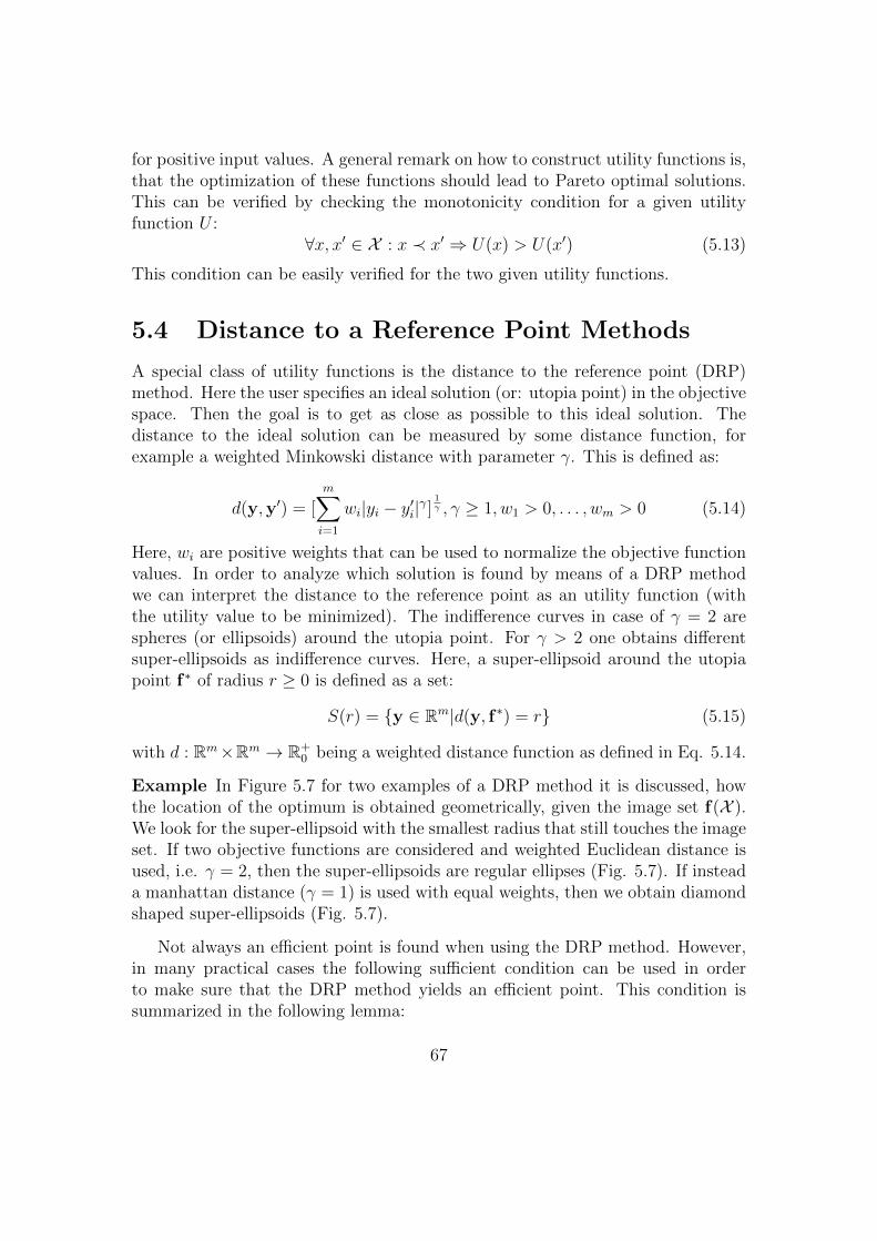
for positive input values. A general remark on how to construct utility functions is,that the optimization of these functions should lead to Pareto optimal solutions.This can be verified by checking the monotonicity condition for a given utilityfunction U :

∀x, x′ ∈ X : x ≺ x′ ⇒ U(x) > U(x′) (5.13)

This condition can be easily verified for the two given utility functions.

5.4 Distance to a Reference Point Methods

A special class of utility functions is the distance to the reference point (DRP)method. Here the user specifies an ideal solution (or: utopia point) in the objectivespace. Then the goal is to get as close as possible to this ideal solution. Thedistance to the ideal solution can be measured by some distance function, forexample a weighted Minkowski distance with parameter γ. This is defined as:

d(y,y′) = [m∑i=1

wi|yi − y′i|γ]1γ , γ ≥ 1, w1 > 0, . . . , wm > 0 (5.14)

Here, wi are positive weights that can be used to normalize the objective functionvalues. In order to analyze which solution is found by means of a DRP methodwe can interpret the distance to the reference point as an utility function (withthe utility value to be minimized). The indifference curves in case of γ = 2 arespheres (or ellipsoids) around the utopia point. For γ > 2 one obtains differentsuper-ellipsoids as indifference curves. Here, a super-ellipsoid around the utopiapoint f∗ of radius r ≥ 0 is defined as a set:

S(r) = y ∈ Rm|d(y, f∗) = r (5.15)

with d : Rm×Rm → R+0 being a weighted distance function as defined in Eq. 5.14.

Example In Figure 5.7 for two examples of a DRP method it is discussed, howthe location of the optimum is obtained geometrically, given the image set f(X ).We look for the super-ellipsoid with the smallest radius that still touches the imageset. If two objective functions are considered and weighted Euclidean distance isused, i.e. γ = 2, then the super-ellipsoids are regular ellipses (Fig. 5.7). If insteada manhattan distance (γ = 1) is used with equal weights, then we obtain diamondshaped super-ellipsoids (Fig. 5.7).

Not always an efficient point is found when using the DRP method. However,in many practical cases the following sufficient condition can be used in orderto make sure that the DRP method yields an efficient point. This condition issummarized in the following lemma:

67

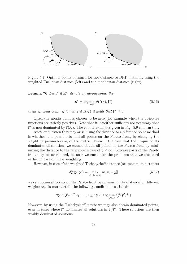
Figure 5.7: Optimal points obtained for two distance to DRP methods, using theweighted Euclidean distance (left) and the manhattan distance (right).

Lemma 76 Let f∗ ∈ Rm denote an utopia point, then

x∗ = arg minx∈X

d(f(x), f∗) (5.16)

is an efficient point, if for all y ∈ f(X ) it holds that f∗ y.

Often the utopia point is chosen to be zero (for example when the objectivefunctions are strictly positive). Note that it is neither sufficient nor necessary thatf∗ is non-dominated by f(X ). The counterexamples given in Fig. 5.9 confirm this.

Another question that may arise, using the distance to a reference point methodis whether it is possible to find all points on the Pareto front, by changing theweighting parameters wi of the metric. Even in the case that the utopia pointsdominates all solutions we cannot obtain all points on the Pareto front by mini-mizing the distance to the reference in case of γ <∞. Concave parts of the Paretofront may be overlooked, because we encounter the problems that we discussedearlier in case of linear weighting.

However, in case of the weighted Tschebycheff distance (or: maximum distance)

d∞w (y,y′) = maxi∈1,...,m

wi|yi − y′i| (5.17)

we can obtain all points on the Pareto front by optimizing the distance for differentweights wi. In more detail, the following condition is satisfied:

∀y ∈ YN : ∃w1, . . . , wm : y ∈ arg miny′∈Y

d∞y (y′, f∗)

However, by using the Tschebycheff metric we may also obtain dominated points,even in cases where f∗ dominates all solutions in f(X ). These solutions are thenweakly dominated solutions.

68

Figure 5.8: In the left figure we see and example for a utopia point which is non-dominated by the image set but the corresponding DRP method does not yielda solution on the Pareto front. In the right figure we see an example where anutopia point is dominated by some points of the image set, but the correspondingDRP method yields a solution on the Pareto front.

Figure 5.9: In the left figure we see and example where an non-dominated pointis obtained using a DRP with the Tschebychev distance. In the right figure we seean example where also dominated solutions minimize the Tschebychev distance tothe reference point. In these cases a non-dominated solution may be missed bythis DRP method if it returns some single solution minimizing the distance.

69

In summary, distance to a reference point methods can be seen as an alternativescalarization approach to utility function methods with a clear interpretation ofresults. They require the definition of a target point (that ideally should dominateall potential solutions), and also a metric needs be specified. We note, that theEuclidean metric is not always the best choice. Typically, the weighted Minkowskimetric is used as a metric. The choice of weights for that metric and the choice ofγ can significantly influence the result of the method. Except for the Tschebycheffmetric, it is not possible to obtain all points on a Pareto front by changing theweights of the different criteria. The latter metric, however, has the disadvantagethat also weakly dominated points may be obtained.

70

Chapter 6

Transforming Multicriteria intoConstrained Single-CriterionProblems

This chapter will highlight two common approaches for transforming Multicrite-ria into Constrained Single-Criterion Problems. In Compromise Programming (orε-Constraint Method), m− 1 of the m objectives are transformed into constraints.Another approach is put forward in the so-called goal attainment and goal pro-gramming method. Here a target vector is specified (similar to the distance to areference point methods), and a direction is specified. The method searches forthe best feasible point in the given direction. For this a costraint programmingtask is solved.

6.1 Compromise Programming or ε-Constraint

Methods

In compromise programming we first choose f1 to be the objective function thathas to be solved with highest priority and then re-state the original multicriteriaoptimization problem (Eq. 1.11):

f1(x)→ min, f2(x)→ min, . . . , fm(x)→ min (6.1)

into the single-criterion constrained problem:

f1(x)→ min, f2(x) ≤ ε2, . . . , fm(x)→ εm. (6.2)

In figure 6.1 the method is visualized for the bi-criteria case (m = 2). Here, itcan be seen that if the constraint boundary shares points with the Pareto front,

71

Figure 6.1: Compromise Programming in the bi-criteria case. The second objectiveis transformed into a constraint.

these points will be the solutions to the problem in Eq. 6.2. Otherwise, it isthe solution that is the closest solution to the constraint boundary among allsolutions on the Pareto-front. In many cases the solutions are obtained at pointsx where all objective function values fi(x) are equal to εi for i = 1, . . . ,m. Inthese cases, we can obtain optimal solutions using the Lagrange Multiplier methoddiscussed in chapter 4. Not in all cases the solutions obtained with the compromiseprogramming method are Pareto optimal. The method might also find a weaklydominated point, which then has the same aggregated objective function valuethan some non-dominated point. The construction of an example is left as anexercise to the reader.

The compromise programming method can be used to approximate the Paretofront. For a m dimensional problem a m−1 dimensional grid needs to be computedthat cover the m − 1 dimensional projection of the bounding box of the Paretofront. Due to Lemma 63 given m − 1 coordinates of a Pareto front, the m-thcoordinate is uniquely determined as the minimum of that coordinate among allimage vectors that have the m − 1 given coordinates. As an example, in a 3-Dcase (see Figure 6.2) we can place points on a grid stretching out from the minimalpoint (fmin1 , fmax1 ) to the maximal point (fmin2 , fmax2 ) . It is obvious that, if thegrid resolution is kept constant, the effort of this method grows exponentially withthe number of objective functions m.

72

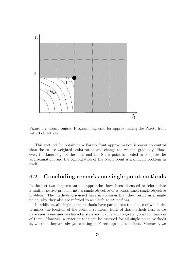
Figure 6.2: Compromised Programming used for approximating the Pareto frontwith 3 objectives.

This method for obtaining a Pareto front approximation is easier to controlthan the to use weighted scalarization and change the weights gradually. How-ever, the knowledge of the ideal and the Nadir point is needed to compute theapproximation, and the computation of the Nadir point is a difficult problem initself.

6.2 Concluding remarks on single point methods

In the last two chapters various approaches have been discussed to reformulatea multiobjective problem into a single-objective or a constrained single-objectiveproblem. The methods discussed have in common that they result in a singlepoint, why they also are referred to as single point methods.

In addition, all single point methods have parameters the choice of which de-termines the location of the optimal solution. Each of this methods has, as wehave seen, some unique characteristics and it different to give a global comparisonof them. However, a criterion that can be assessed for all single point methodsis, whether they are always resulting in Pareto optimal solutions. Moreover, we

73

investigated whether by changing their parameters all points on the Pareto frontcan be obtained.

To express this in a more formal way we may denote a single point method bya function A : P × C 7→ Rm ∪ Ω, where P denotes the space of multi-objectiveoptimization problems, C denotes the parameters of the method (e.g. the weightsin linear weighting). In order to classify a method A we introduce the followingtwo definitions:

Definition 77 Proper single point methodA method A is called proper, if and only if for all p ∈ P and c ∈ C either phas a solution and the point A(p, c) is Pareto optimal or p has no solution andA(p, c) = Ω.

Definition 78 Exhaustive single point methodA method A is called exhaustive if for all p ∈ P : YN(p) ⊆

⋃c∈C A(p, c), where

YN(p) denotes the Pareto front of problem p.

In table ?? a summary of the properties of methods we discussed: In thefollowing chapters on algorithms for Pareto optimization the single point methodsoften serve as components of methods that compute the entire Pareto front, or anapproximation to it.

74

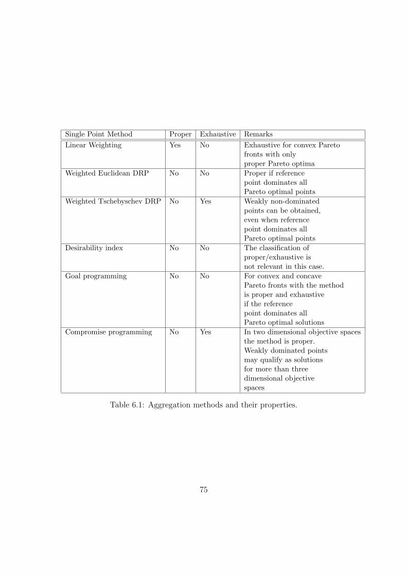
Single Point Method Proper Exhaustive Remarks

Linear Weighting Yes No Exhaustive for convex Paretofronts with onlyproper Pareto optima

Weighted Euclidean DRP No No Proper if referencepoint dominates allPareto optimal points

Weighted Tschebyschev DRP No Yes Weakly non-dominatedpoints can be obtained,even when referencepoint dominates allPareto optimal points

Desirability index No No The classification ofproper/exhaustive isnot relevant in this case.

Goal programming No No For convex and concavePareto fronts with the methodis proper and exhaustiveif the referencepoint dominates allPareto optimal solutions

Compromise programming No Yes In two dimensional objective spacesthe method is proper.Weakly dominated pointsmay qualify as solutionsfor more than threedimensional objectivespaces

Table 6.1: Aggregation methods and their properties.

75

Part II

Algorithms for ParetoOptimization

76

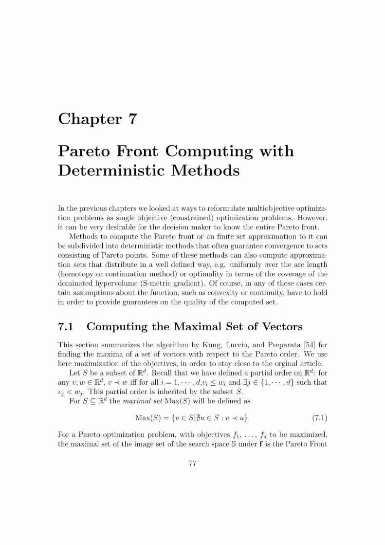
Chapter 7

Pareto Front Computing withDeterministic Methods

In the previous chapters we looked at ways to reformulate multiobjective optimiza-tion problems as single objective (constrained) optimization problems. However,it can be very desirable for the decision maker to know the entire Pareto front.

Methods to compute the Pareto front or an finite set approximation to it canbe subdivided into deterministic methods that often guarantee convergence to setsconsisting of Pareto points. Some of these methods can also compute approxima-tion sets that distribute in a well defined way, e.g. uniformly over the arc length(homotopy or continuation method) or optimality in terms of the coverage of thedominated hypervolume (S-metric gradient). Of course, in any of these cases cer-tain assumptions about the function, such as convexity or continuity, have to holdin order to provide guarantees on the quality of the computed set.

7.1 Computing the Maximal Set of Vectors

This section summarizes the algorithm by Kung, Luccio, and Preparata [54] forfinding the maxima of a set of vectors with respect to the Pareto order. We usehere maximization of the objectives, in order to stay close to the orginal article.

Let S be a subset of Rd. Recall that we have defined a partial order on Rd: forany v, w ∈ Rd, v ≺ w iff for all i = 1, · · · , d,vi ≤ wi and ∃j ∈ 1, · · · , d such thatvj < wj. This partial order is inherited by the subset S.

For S ⊆ Rd the maximal set Max(S) will be defined as

Max(S) = v ∈ S|@u ∈ S : v ≺ u. (7.1)

For a Pareto optimization problem, with objectives f1, . . . , fd to be maximized,the maximal set of the image set of the search space S under f is the Pareto Front

77

(PF) of that problem.For all d ≥ 1 a lower and upper bound of finding the maximal subset of a set

will be given. For the proposed algorithms the time complexity will be derivedas well. For d = 2 or 3 we will describe efficient algorithms and in that case alsoprove their efficiency.

The number of comparisons an algorithm A needs for computing the maximalset of S will be denoted with cd(A, S). The time complexity of a d-dimensionalproblem in terms of n = |S| is estimated as:

Td(n) = minA∈A

maxS⊂nRd

cd(A, S) (7.2)

Here A is the set of all algorithms and ⊂n is the subset operator with therestriction that only subsets of size n are considered.

For y ∈ Rd we denote the vector (y2, · · · , yd) by y∗. In other words, the firstcoordinate is discarded.

We denote by pi the projection of S to the i-th coordinate (for any fixed i ∈1, · · · , d).

Definition 79 Let A ⊆ Rd and y ∈ S. Then y ≺ A iff ∃a ∈ A such that y ≺ a

Lemma 80 Let A ⊆ Rd and y ∈ S. Then y ≺ A iff y ≺ Max(A).

A prototype of the algorithm for computing the maximal elements (PF) of S isas follows. In order to present the ideas more clearly we assume y(i), i = 1, · · · ,mto be mutually different in each coordinate. We shall address equality in some (orall coordinates) separately. It is clear that in case d = 2, the sets Ti contain oneelement and for updates only one comparison is used, so the time complexity ofthe algorithm in this case is n log n. (The sorting requires n log n steps while theloop requires n comparisons.)In case d = 3, the maintenance of the sets Ti is done by a balanced binary treewith keys the second coordinate of the vectors y(i). A crucial step in the loop is toupdate the T i given y(i+1). First determine the element in T (i) that precedes yi inits second coordinate. Then determine the elements that are dominated by y(i) byvisiting the leaves of the search tree in descending order of the second coordinates,and stop when the first visited element exceeds the third coordinate of y(i+1) inits own third coordinate. Discard all visited points, as they are dominated in allthree coordinates by yi+1.

Note that in this case the third coordinate is also sortedBy Lemma 80 we can replace the test y(i)∗ ≺ Ti−1 in step 5 of Algorithm 3 by

the test y(i)∗ ≺ Max (Ti−1).A variation on Algorithm 3 is to mark an element as maximal as you go along

and work with Max (Ti−1). Note that the algorithm is ’monotone’: once for an

78

Figure 7.1: In order to find out whether or not a point y(i) is dominated, firstthe successor in the 2nd coordinate in ascending order is determined. Using abalanced search tree this step takes O(log n) time. If the third coordinate of thesuccessor exceeds the third coordinate of the point y(i) then y(i) is dominated anddiscarded. Otherwise, the algorithm deletes all points that are dominated by y(i)

(points in the shaded area) and insert y(i) into the non-dominated set and updatesthe balanced tree. The update of the balanced tree is done by moving throughthe set of points in direction of decreasing second coordinate (and consequentlyincreasing third coordinate) until the third coordinate of y(i) is exceeded. Thepoints visited on that path are deleted and finally y(i) is inserted into the balancedsearch tree. As each node enters the tree and leaves the tree at most once in theentire n runs of the described algorithm, the total running time will not exceedO(n log n).

79

Algorithm 3 Prototype Algorithm for Computing PF of a finite set S

1: input: S = y(1), · · · ,y(k) ⊆k Rd and k ∈ NNB We assume the y(i) to be mutually different in each coordinate.

2: View the elements S as a sequence and sort the elements of this sequence bythe first coordinate in descending order: y(1),y(2), · · · ,y(k−1),y(k) is now suchthat

p1(y(1)) > p1(y

(2)) > · · · > p1(y(k−1)) > p1(y

(k))

3: i← 1;4: T0 ← ∅; The Ti are sets of (d− 1)-dim vectors 5: for all i = 1, . . . , k do6: if y(i)∗ ≺ Ti−1 then7: Ti ← Ti−18: else9: Ti ← Max (Ti−1 ∪ y(i)∗) and mark y(i) as maximal.

10: end if11: end for

element its star is admitted to Ti it is clearly maximal (and the star will survivein future Ti.

The prototype can be specialized by describing which choices have been madefor the test y(i)∗ ≺ Ti−1 and for the building of the Ti.

80

Chapter 8

Evolutionary MulticriterionOptimization

Evolutionary Algorithms (EA) are stochastic search and machine learning heuris-tics, inspired by theories of biological evolution, most prominently by the so-called modern evolutionary synthesis that combines natural selection and genetics(see [27]). Traditionally, EA have been categorized into three subfields: Genetic Al-gorithms (GA) [37] (mainly binary representations), Evolution Strategies (ES ) [10](mainly continuous representations) and Evolutionary Programming (EP) [35](arbitrary representations). Nowadays, the boundaries between these subfieldsbecame more fluid and the methods are often grouped together using the termEvolutionary Algorithms (see [3]).

EA are used for machine learning and as simulation models in biology [37],but their major field of application is surely systems optimization. This class ofmethods does not require derivatives of the functions defining the problem and itis relatively robust and flexible for solving nonlinear optimization problems, dueto the stochastic search operators involved in the algorithmic definition. Empiricalresults suggest that on nonsmooth and nonconvex problems EA can outperformclassical deterministic methods (see [75]). For continuous optimization, advancedEA, such as the Covariance Matrix Adaptation Evolution Strategy (CMA-ES ) [40],are nowadays considered to be state-of-the-art methods.

Evolutionary Multiobjective Optimization (EMO) applies EA for the solutionof MOO problems. After first pioneering work in the eighties [74] and in theearly nineties [36, 55], these methods received strong attention during the lasttwo decades [17]. What has emerged as a side-branch of the evolutionary com-putation community is today considered as a more independent field of research,at the intersection of Evolutionary Algorithms, Metaheuristics, and MulticriteriaDecision Making. In addition, EMO methods became popular for solving prac-tical problems in multiobjective optimization (see, e.g., Branke et al. [13]). The

81

major focus in EMO has been the computation of finite approximations to Paretooptimal sets and Pareto fronts. Some algorithms, such as the second versions ofthe Nondominated Sorting Genetic Algorithm (NSGA-II ) [25] and the StrengthPareto Evolutionary Algorithm (SPEA2 ) [87], became popular techniques for thistask and will be reviewed here. We will also review more recent trends, exemplifiedby algorithms such as the hypervolume-based S-metric Selection EMO algorithm(SMS-EMOA) [29] and the Multiobjective CMA-ES (MO-CMA-ES ) [46], the lat-ter specially designed for solving continuous optimization problems.

8.1 Single Objective Evolutionary Algorithms

In EA mathematical objects are often referred to by biological metaphors, suchas individual (solution), population (tuple of solutions), and fitness (objectivefunction value or rank of an individual, within a population).

This adds a layer of abstraction to the algorithmic description, which canpresent different instantiations. As an example, an individual could representa point in 0, 1n, a point in Rn, or even an instance of a dynamic data-structure.In the sequel, however, the focus will be on continuous search spaces, meaningthat individuals are represented as points in Rn and populations are considered tobe fixed-cardinality multisets of individuals.

Algorithm ?? describes a generic EA for single objective optimization. Usingthe subsequently discussed genetic operators, the stochastic transition is designedin such a way that the expected value of the objective function of the populationindividuals improves over time. Within the framework of EA one distinguishesbetween parent populations Xt (of size µ > 0) and offspring populations Ot (ofsize λ > 0), at iterations t ∈ 0, 1, 2, . . . . The iteration counter is denoted byt to emphasize that Xtt∈N could be regarded as the trajectory in (Rn)µ of astochastic process indexed in time. The offspring population, Ot, is an interme-diate population that is generated by the variation operators (recombination andmutation) from the individuals of the parent population Xt. The next generationparent population, Xt+1, will be selected from the union of the parent and offspringpopulations, considering the fitness of the individuals.

The initialization of an EA is typically done in an uniform random manner, withrespect to the space of feasible solutions Ω. Important instantiations of matingselection are:

• Random selection: randomly selecting parents, in which case the sameparent can be repeatedly chosen. This selection type is typically applied inES [10].

• Tournament selection: two (or more) individuals are selected randomly

82

Generic Evolutionary Algorithm (EA)

InitializationDefine all required algorithmic parameters (parent population size (µ),number of recombination partners (ρ), number of offsprings (λ), mutationstrength (σ), etc.) and set the generation (iteration) counter t = 0. Initializethe parent population, X0, and assign a fitness to each of its µ individuals,based on the corresponding objective function value (and, possibly, othercriteria).

For t = 0, 1, 2, . . .

• Mating selection: Select ρ individuals in Xt, that will serve as ‘tem-plates’ for the individuals in Xt+1.

• Recombination: Combine the information of the selected individuals(e.g. by means of random crossover or of averaging) in order to createa new population, Ot, of λ offspring individuals.

• Mutation: Perturb (some of) the offspring individuals in Ot by meansof small random modifications.

• Fitness assignment: Evaluate the fitness of each offspring individual,considering the corresponding objective function value (and, possibly,other criteria).

• Environmental selection: Select individuals from the offspring pop-ulation Ot (and, possibly, also from the parent population Xt), in orderto form the next generation parent population Xt+1 (of size µ).

83

from the parent population and the individual with the best fitness will bekept. This selection type is typically applied in EP [35].

• Roulette wheel selection: Individuals are selected with a probability orfrequency that is proportional to their fitness or rank in the population. Thisselection type is typically applied in GA [37].

Besides the selection of individuals to be recombined and/or mutated, the envi-ronmental selection is used to compute the population Xt+1 from the offspringpopulation Ot, and also possibly from Xt. The (µ + λ)-selection and the (µ, λ)-selection strategies are distinguished:

• (µ + λ)-selection: The best µ solutions in the union Xt ∪ Ot are selected.Because the size of this union equals µ+ λ, this selection is termed (µ+ λ)-selection. For instance, a (µ + 2)-selection denotes a selection of the µ bestsolutions from the union of a set of µ parents and a set of 2 offsprings.

• (µ, λ)-selection: The best µ solutions among the λ offspring solutions, Ot,are selected, meaning that the previous parent population Xt is not consid-ered in the selection. In this case µ ≤ λ must hold.

Offspring individuals are generated by means of recombination and mutationoperators. Recombination is used to combine information of two or more parents inorder to form an offspring, for instance by averaging or by crossover. Theoretically,it has been shown that for decomposable functions recombination can enhance thefrequency of parts of the individuals that contribute to a good fitness [37] anddecrease deteriorating effects of mutation [10]. Recombination also serves to creatediversity and to exchange information across a population. In the context of EMO,it can create solutions that lie in the gaps between existing solutions.

Mutation modifies an individual by a small random perturbation. For instance,a Gaussian mutation of a given individual x ∈ Rn corresponds to:

x′ = x+ σz with z ∼ Normal(0,Σ),

where Normal(0,Σ) denotes a multivariate Gaussian distribution with mean 0 andcovariance matrix Σ, and σ is a scaling factor. In ES it is common to adapt thescaling factor, σt, across the different generations. For this, several control schemeswere proposed. One of these proposals is based on success-rates (e.g. [75, 10, 48]).In ES following a 1/τth-success rule means that σ is multiplied by a constant0 < ξ < 1, if the success-rate after a fixed epoch of c > τ iterations is below 1/τ ,and divided by ξ otherwise. A value of τ = 5 proved to be a good default settingfor a range of problems and is used as a standard setting – hence the name 1/5th

84

success rule [75]. Alternatively, mutative self-adaptation and derandomized self-adaptation are widely used. Here σ (or even Σ itself) gets part of the individualand undergoes an evolutionary process. For details, see [10] and [40], respectively.

The CMA-ES [40] also adapts the covariance matrix Σ during the generations,adjusting the mutation to the local quadratic form of the objective function. Forthis, it integrates the sample path from the history of the individuals (evolutionpath). In particular, for continuous objective functions with an high conditionnumber and correlation between the optimization variables, the CMA-ES is oftenpreferred to other ES instantiations.

The behaviour of almost all evolutionary algorithms can be modelled as anhomogeneous Markovian process with kernel K(X, A), describing the transitionprobability of a given population X ∈ (Rn)µ entering in some set A ⊂ (Rn)µ in thesubsequent generation. For instantiations of transition kernels for EA see [71].

Based on this, conditions for complete convergence of EA can be established.Complete convergence is a strong type of probabilistic convergence. Lucacs [59]defines it as:

Definition 81 (Complete convergence) Let Y denote a random variable (whichmight as well be a constant) and Ytt∈N a sequence of random variables definedon a probability space (B,A, P ). Then Ytt∈N is said to converge completely toY , if for any ε > 0:

limt→∞

t∑i=1

P|Yi − Y | > ε <∞.

Next, let us define b : ℘((Rn)µ)→ R as the function that assigns to a populationin (Rn)µ the objective function value of its best individual. Moreover, for ε > 0and f∗ the global minimum of the objective function f (provided it exists), wedefine Aε = X ∈ (Rn)µ | b(X) ≤ f∗ + ε. Using these definitions, we can state thefollowing result.

Theorem 82 (Corollary 6.3 in [71]) An EA whose Markovian kernel satisfiesthe condition K(X, Aε) ≥ θ > 0, for all X ∈ Acε = (Rn)µ \ Aε, and K(X, Aε) = 1for any X ∈ Aε, for any ε > 0, will converge completely to the global minimum ofthe real valued function f , regardless of the initial distribution of the individuals.

It is interesting to note that the condition on the Markovian kernel is satisfiedfor ES using a (µ+λ)-selection strategy, considering a positive definite covariancematrix Σ and bounded scaling factors 0 < σmin < σ < σmax < ∞, provided theyare applied to bound constrained problems with a continuous objective function(see [71]).

On simple quadratic functions, Beyer [9] derived expressions showing a linearconvergence rate of ES with optimally adapted step sizes, using a (µ + λ) or

85

(µ, λ)-selection strategies, for a dimension n → ∞. For a summary, see also [10].Empirically, it was shown that most of these results already hold for n of moderatesize. Jagerskupper [48] proved that, on quadratic forms, ES using a (1+1)-selectioncombined with a 1/5th success rule for step-size adaptation converge linearly withoverwhelming probability, that is, the probability that the distance to the optimumdoes not halve in O(n) iterations approaches zero with exponential rate in n.

More than analysing the convergence properties of classical EA, proposals weremade to change the design of some methods belonging to this class, in order toenforce convergence to a stationarity point. Hart [43] introduced a variant ofES, called Evolutionary Pattern Search, which generalizes the Stochastic PatternSearch method proposed in [42]. The new algorithm includes in the mutationoperator a set of search directions which forms a positive basis for Rn. It usesupdate schemes similar to the ones of DSM, but opposed to them considers apopulation of search points and randomizes some of the procedures.

Recently, Diouane et al. [26] have also proposed a slightly modified versionof CMA-ES, and other similar ES instantiations. For objective functions whichare locally Lipschitz continuous, they have proved the convergency for a Clarkestationarity point, independently of the points considered in initialization. Theproposed modification consists in strategies to update the step size parameterbased on different sufficient decrease conditions.

Besides these theoretical results, we note that in the field of EA, systematicexperimental research plays an important role in the algorithmic development.See [6], for a treatise.

8.2 Evolutionary Multiobjective Optimization

Shifting the attention from single to multiobjective EA means, in the first place,to focus in the selection operator design. While in single objective optimizationselection procedures can be directly based on the objective function value and inrankings depending on it, in MOO, where there are partially ordered objectivefunction vectors, fitness assignment or ranking is not that straightforward. Threemain alternatives can be identified in the EMO literature, which were proposed inthe given order:

1. Scalarization-based approaches: The objective function vectors are ag-gregated into a single scalar value, using simple weighting or an utility func-tion. In order to compute different solutions, the parameters of the utilityfunction are dynamically or randomly changed. Examples are the VectorEvaluated Genetic Algorithm (VEGA) [74] and the Random Objective Se-lection Evolutionary Algorithm (ROSEA) [72], the latter based on an earlierframework proposed by [55] for multiobjective ES.

86

2. Nondominance and diversity approaches: Solutions are computed basedon dominance and diversity. Often, nondominance is prioritised to diversityto achieve convergence to a set of Pareto optimal solutions. Examples ofthis approach are the Nondominated Sorting Genetic Algorithm (version 2)NSGA-II [25] and the Strength Pareto Evolutionary Algorithm (version 2)SPEA2 [87].

3. Indicator-based approaches: In this case, a selection is performed amongsets, favouring the ones which present a better performance indicator. Thisperformance indicator should measure the quality of a set as an approxi-mation to the Pareto front of the problem. Indicator based evolutionaryalgorithms were suggested as an algorithm class in [86], being the hyper-volume indicator often chosen as performance indicator. The HypervolumeEstimation Algorithm HypE [4] and the S-Metric Selection EvolutionaryMultiobjective Optimization Algorithm SMS-EMOA [29] are instantiationsof indicator based evolutionary algorithms. The same happens for a com-mon variant of the Multiobjective Covariance Matrix Adaptation EvolutionStrategy MO-CMA-ES [46, 83].

Aggregation based methods were described in the first pioneering papers onEMO. In VEGA [74], weights of the objective functions are randomly changed,promoting diversity inside the population and its better coverage of the Paretofront. With the same purpose, ROSEA [72] changes randomly the objective func-tion used in the selection. Rudolph [72] analysed the convergence properties ofROSEA for a quadratic MOO problem, establishing a sublinear convergence rate.The major drawback of these aggregation based approaches relies on their inabil-ity to capture concave parts of the Pareto fronts. Thus, they have been widelyabandoned in the EMO field.

The selection mechanisms incorporated in the NSGA, its successor NSGA-II,and SPEA2 are prominent examples of the second selection principle: a com-bination of nondominance and diversity. Basically, these algorithms differ in theranking, based on nondominance level, and the subsequent diversity measurement.A more detailed discussion follows in Subsection 8.2.1. Other algorithms thatfall into this class are the Pareto Archived Evolution Strategy (PAES) [52] andthe ε-MOEA [24], which partition the objective function space into grid cells tomeasure diversity. A stronger focus on variation/sampling operators design gaverise to algorithms such as the Multiobjective Estimation of Distribution Algo-rithm [12], the Differential Evolutionary Multiobjective Optimization (DEMO) [70]and the Multiobjective Covariance Matrix Adaptation Evolution Strategy (MO-CMA-ES ) [46, 83].

The SMS-EMOA [29] and HypE [4] can be seen as instantiations of indicator-based methods, the design of which is directly governed by a performance indica-

87

tor. Because this design principle is a recent trend in the advancement of EMOalgorithms, we will devote Subsection 8.2.2 to it. The hypervolume indicator wasalso proposed as a selection criterion in MO-CMA-ES [46, 83]. However, the maincontribution present in this method is to generalize the single objective CMA-ESto MOO. We will discuss it in more detail in Subsection 8.2.3.

Another line of algorithmic designs has focused on interacting models of evo-lution and co-evolution, inspired by the predator-prey approaches. Here, differ-ent objectives are represented by different prey-individuals, that simultaneouslyperform the selection on different aggregated objective functions (see [56, 39]).Though these bio-inspired algorithms provide flexibility and robustness in practi-cal settings [39], their convergence properties remain widely unexplored.

8.2.1 Algorithms Balancing Dominance and Diversity

NSGA-II [25] is probably the most commonly used EMO algorithm, partially dueto its straightforward, yet effective, design. NSGA-II is a GA considering a (µ+µ)-selection strategy, and binary tournament for mating. Its main innovation, asopposed to single objective optimization algorithms, consists in ranking solutionsbased on a vector valued fitness function, and thereby at the same time considersdomination and diversity. Ranking is done in two steps:

1. Nondominated sorting: In this step the union of the parent and offspringpopulations Q ∈ Ωµ+µ is partitioned into Q(1), . . . , Q(k), where Q(1) is theset of nondominated solutions in Q, and Q(i+1) is recursively defined as thenondominated set of Q − ∪ij=1Q

(j), for i = 1, 2, . . .. Nondominated sorting

will result in 0 < κ ≤ |Q| nonempty sets Q(1), . . . , Q(i), . . . ,Q(κ). The indexi of the set Q(i) determines the nondominance level of the solutions in Q(i).

2. Crowding distance sorting: Each set Q(i), i ∈ 1, . . . , κ, obtainedby nondominated sorting, can be further sorted by means of the crowd-ing distance. The crowding distance measures the contribution of a solu-tion to the diversity of a population – the higher the crowding distancethe better the solution. For some q ∈ Q(i) it is given by crowd(q) =∑n

d=1(∆+d (q,Q(i)) + ∆−d (q,Q(i))), where ∆+

d (q,Q(i)) denotes the next higherd-th coordinate of a point q′ ∈ Q(i) − q and ∆−d (q,Q(i)) denotes the nextlower d-th coordinate of a point q′′ ∈ Q(i) − q.

A crucial design principle of NSGA-II is to prioritize on the nondominancelevel. Only in case of incomparable solutions it favours those that better con-tribute to diversity. In common implementations of NSGA-II either classical ge-netic operators are used or – in the canonical version for continuous search spaces -

88

simulated binary crossover in combination with polynomial mutation is considered.For details on these operators we refer to the literature [25].

Although NSGA-II is an elitist algorithm, it was shown that it can deteriorate,meaning that after some generations the set of approximate solutions might bestrictly worse then the previous population [30]. Nevertheless, for population withlarger sizes the effects of deterioration tend to disappear[30]. In fact, in a widerange of benchmarks and application problems, NSGA-II was reported to yieldgood approximations of Pareto fronts, in particular for the 2-D case. A similaralgorithm to NSGA-II that also enjoys wide popularity is SPEA2 [87]. Instead ofusing nondominated sorting for ranking in the first step, it computes the strengthof individuals, by counting how many other individuals it dominates and by howmany individuals it is dominated. A clustering method is then used as a selectioncriterion among individuals of equal strength, in order to promote diversity.

8.2.2 Indicator-based Algorithms

In the algorithms belonging to this class, selection strategies use performance in-dicators to measure the quality of different sets, as approximations to the Paretofront of a given problem. To do it, without the knowledge of the actual Paretofront, the hypervolume indicator was suggested, due to its favorable properties[88].Given a reference point r ∈ Rm, that is dominated by all the approximations con-sidered for the Pareto front (or at least by the actual Pareto front of the problem),the hypervolume indicator measures the size of the space that is dominated by theset approximating the Pareto front and upper bounded by the considered referencepoint.

Definition 83 (Hypervolume indicator) The hypervolume indicator (or S-metric,from ‘Size of space covered’) for some (approximation) set A ⊂ Rm and a referencepoint r ∈ Rm that is dominated by all the points in A is defined as:

HI(A) = Volb ∈ Rm|b ≤ r ∧ ∃a ∈ A : a ≤ b = Vol(∪a∈A[a, r])

Here Vol(.) denotes the Lebesgue measure of a m-dimensional set of points, and[a, r] denotes the interval box with lower corner a and upper corner r.

In 2-D this is simply the covered area, and in 3-D the covered volume (see Figure 8.1for examples). For reviewing some important properties related to this indicator,lets us introduce a comparison operator between sets.

Definition 84 Given two nondominated sets A and B, A is better than B, whichis represented by A ≺ B, if

∀b ∈ B : ∃a ∈ A : a ≤ b (componentwise) and ∃b ∈ B : ∃a ∈ A : a ≺ b.

89

(Error converting to EPS. Consult Lieuwe)

Figure 8.1: Hypervolume indicator in two dimensions for a set A = a1, ..., a4 ⊂R2 (left) and in three dimensions for a set Y = y1, . . . , y5 ⊂ R3 (right).

The hypervolume indicator is, up to an isomorphism, the only known indicatorthat presents the following monotonicity property.

Lemma 85 (Zitzler et al. [88]) For two nondominated sets A and B with A ≺B and ∀x ∈ A ∪B : x ≺ r for a reference point r it holds that HI(A) > HI(B).

This property makes sure that strict improvements of approximating sets willresult in an increment of the hypervolume. Moreover, the following property canbe established for the hypervolume indicator.

Lemma 86 (Zitzler et al. [88]) Let ≺ be defined as in Definition 84, and A andB denote two nondominated sets with ∀x ∈ A ∪ B : x ≺ r for a reference point rand HI(A) > HI(B). Then B 6≺ A.

Basically, the lemma states that measuring by means of the hypervolume indicatorwill never favour an approximation set that is strictly worse than the another one.This implies that search strategies that generate a sequence of approximation setsor populations with monotonously increasing hypervolume will not deteriorate [30].

Indicator-based EMO algorithms use indicators that measure the quality of theeventually obtained set to directly guide the selection [86]. The idea is instantiatedin the S-Metric Selection Evolutionary Multiobjective Optimization Algorithm(SMS-EMOA) [29], which considers a (µ + 1)-selection scheme. Like in NSGA-II, the ranking procedure could be subdivided into two steps.

• Nondominated sorting: The first step is nondominated sorting (like dis-cussed for NSGA-II ), giving rise to partitions of equal nondominance levelQ(1), . . . , Q(κ).

• Hypervolume-based ranking: The partition with worst nondominancelevel, namely Q(κ), is reduced to a subset of |Q(κ)| − 1 solutions. The subsetthat covers the biggest hypervolume survives.

The design of the algorithm makes sure that, regardless of the stochastic real-ization, the hypervolume of the approximating set will either grow or remain thesame. From Lemma 86 it can be concluded that the search cannot deteriorate to

90

strictly worse Pareto front approximations, as this might be the case in NSGA-IIand SPEA2.

The choice of a (µ + 1)-selection scheme is motivated by the efficiency of thesubset selection for this special case. It suffices to delete the solution in Q(κ)

that presents the smallest contribution to the corresponding hypervolume. Thecontribution of a point a ∈ A ⊂ Rm to the hypervolume defined by the set A ismeasured by:

∆HI(a,A) = HI(A)− HI(A− a) (8.1)

The computation of all contributions can be accomplished in asymptotically op-timal time O(|A| log |A|), for m = 2 and m = 3 [31]. For higher dimensions, upto now, only algorithms with polynomial, but superquadratical, running time areknown [7]. This limits the applicability of SMS-EMOA to problems with only amoderate number of objective functions.

Recently, several results have been obtain on the distribution of points thatmaximizes the hypervolume indicator. A set is said to be µ-optimal relatively tothe hypervolume indicator if it presents the biggest hypervolume among all setsof size µ. It has been shown that, if the size of the actual Pareto front is equal orgreater than µ, µ-optimal sets consist of only Pareto optimal points. Moreover, in2-D, when µ → ∞, the set of points maximizing the hypervolume indicator willform a dense subset on the Pareto front [2].

Recent studies have shown that in some cases the SMS-EMOA is not guaranteedto converge to a µ-optimal set (e.g. [1]). This results from its (µ + 1)-selectionscheme. To guarantee convergence to a µ-optimal set, a (µ + λ)-selection withµ ≥ λ that selects the subset of size µ with maximal hypervolume is both sufficientand necessary. For m = 2, an algorithm for subset selection with running timeO(µ3) is available [1], but for m > 2 only algorithms with exponential runningtime are known.

In contrast to SMS-EMOA, the Hypervolume Estimation Algorithm (HypE ) [4]considers a general (µ + λ)-selection scheme, where λ can be bigger than 1. Toaccomplish practical feasible running times, instead of using exact computation inthe subset selection procedures, it applies Monte Carlo sampling for computationsrelated to the hypervolume indicator and a modified fitness assignment. Insteadof only considering contributions of single points to the hypervolume indicator,it also considers joint contributions of two or more points to this indicator. Thevolume of the subspace that is jointly dominated by k points is assigned in equalproportions to the points that dominate it.

As the computational complexity of the hypervolume indicator grows exponen-tially with the number of objective functions [14], and Monte Carlo approximationis less affected by dimensionality, HypE is considered to be a promising algorithmfor MOO with an high number of components for the objective function [4].

91

First convergence results in hypervolume-based optimization were recently ob-tained. Beume et al. [8] introduced an analysis method that allows to generalizeconvergence results for single objective EA to EMO algorithms. Using this method,it has been proved the convergence of SMS-EMOA with a (1 + 1)-selection, andof a modified version of SMS-EMOA with a (µ + 1)-selection, that works withmultiple reference points and considers tournament selection based on pairwisecomparisons. In particular, Beume et al. [8] extended the convergence results ofRudolph [71] and Jagerskupper [48], discussed in Subsection 8.1, to these twoalgorithms.

Whereas earlier theoretical research focused on either very simple discrete prob-lems [57] or in algorithmic designs that do not address diversity maintenance [73],the findings of Beume et al. [8] can be regarded as first results towards convergenceanalysis for common EMO algorithms in continuous problem classes of practicalrelevance. For now, results are still confined to particular, uncommon algorithmicinstantiations, and more general convergence results would be desirable.

8.2.3 Multiobjective Evolution Strategy

While the previously discussed NSGA-II, SPEA2, SMS-EMOA, and HypE can alsobe used in discrete search spaces, the MO-CMA-ES [46] is an EMO method that isespecially designed for continuous optimization, since it is intended to generalizethe single objective CMA-ES to MOO. As in SMS-EMOA, it uses a ranking strat-egy which is firstly based on nondominated sorting and considers contributions ofthe hypervolume indicator (see Definition 83) as a secondary ranking criterion. Itestablishes a complete ordering on the population by prioritising nondominancelevel to hypervolume contribution. Consider a set Q(i), for some i ∈ 1, . . . , κ,with more than two solutions of equal dominance level. The solution q with theminimal hypervolume contribution is ranked worst, then the solution with mini-mal hypervolume contribution is detected from the set Q(i)−q and assigned thesecond worst rank, and so forth.

The CMA-ES and MO-CMA-ES work with a Gaussian mutation operator, forwhich the corresponding covariance matrix Σ is adapted by means of an elaboratedscheme that depends on a evolution path and a success probability. A success isdeclared if an offspring is selected as one of the parents of the next generation. Incase of success the scaling factor σ is decreased, while otherwise it is increased.The path of past evolution steps that led to an offspring is integrated, in order toapproximate a conjugate direction that is used to scale and rotate the shape ofthe distribution represented by the covariance matrix Σ. This way, the mutationdistribution is adapted, allowing to increase the progress rate for near-quadraticforms with high condition numbers.

Updates of the covariance matrix require, at least, quadratic time. Despite

92

this large computational effort, the MO-CMA-ES is an interesting alternative toalgorithms with a fixed covariance matrix, in cases where the scale of the variableslargely differs and search proceeds in directions diagonal to the main coordinateaxes.

A state-of-the-art instantiation with a detailed description of the update proce-dures of the MO-CMA-ES is found in [83]. So far, a theoretical convergence theoryis not available for MO-CMA-ES, though there is empirical evidence of its goodperformance [46]. The improvement of the MO-CMA-ES is still a topic of activeresearch. Interesting developments include the introduction of advanced recombi-nation schemes [82], step-size adaptation schemes [83] and replacement of randommating selection by a selection scheme motivated by reinforcement learning [58].

8.3 Final Remarks

EMO algorithms introduced some interesting concepts, such as indicator-basedselection and randomization. Some of these might also prove to be beneficial fordesign of deterministic MOO methods. Finally, hybrids of deterministic MOOmethods and EMO, as they already exists in single objective optimization, mightyield search algorithms that enjoy at the same time the flexibility and robustnessof EMO algorithms and the deterministic convergence properties of DSM.

93

Chapter 9

Conclusion

This work is an overview on Multicritera Optimization and Decision Analysis.To this end it covered the prevalent trends in the field, including the classicaltheories based on aggregation and the KKT conditions and more modern set-oriented techniques.

The research field is still very active and recently progress is made in thedefinition of methods for other types of orders, including cone orders or Lorenzorders. Another trend is to combine the MCDM field with optimization methodsin order to better meet the needs of practitioners. In practice it will also benecessary to consider human decision making, which is often irrational or basedon subjective criteria.

The search for faster and more reliable algorithms for finding Pareto frontsis also an ongoing endeavour. For instance recently online algorithms are devel-oped for the dynamic update of populations based on, for instance, hypervolume.Such updates can be accomplished much faster than recomputing every iterationfrom scratch. It has for instance been shown by Hupkens and Emmerich thatsingle generations of the 2-D SMS EMOA can be accomplished in logarithmictime complexity, making them very competitive in terms of computational effortto NSGA-II. Also, more recently set oriented versions of classical numerical algo-rithms such as gradient descent and Newton’s methods were formulated on sets,which exhibit super-linear convergence speed, albeit being less robust than evolu-tionary methods.

94

Bibliography

[1] A. Auger, J. Bader, D. Brockhoff, and E. Zitzler. Investigating and exploit-ing the bias of the weighted hypervolume to articulate user preferences. InGECCO ’09: Proceedings of the 11th Annual Conference on Genetic and Evo-lutionary Computation, pages 563–570. ACM, 2009.

[2] A. Auger, J. Bader, D. Brockhoff, and E. Zitzler. Theory of the hypervolumeindicator: optimal µ-distributions and the choice of the reference point. InFOGA ’09: Proceedings of the 10th ACM SIGEVO Workshop on Foundationsof Genetic Algorithms, pages 87–102. ACM, 2009.

[3] T. Back and H. P. Schwefel. An overview of evolutionary algorithms forparameter optimization. Evolut. Comput., 1:1–23, 1993.

[4] J. Bader and E. Zitzler. HypE: An algorithm for fast hypervolume-basedmany-objective optimization. Evolut. Comput., 19:45–76, 2011.

[5] S. Bandyopadhyay, S. K. Pal, and B. Aruna. Multiobjective GAs, quantativeindices, and pattern classification. IEEE Trans. on Syst., Man, and Cybern.– Part B: Cybernetics, 34:2088–2099, 2004.

[6] T. Bartz-Beielstein. Experimental Research in Evolutionary Computation:The New Experimentalism. Springer, 2006.

[7] N. Beume. S-Metric calculation by considering dominated hypervolume asKlee’s measure problem. Evolut. Comput., 17:477–492, 2009.

[8] N. Beume, M. Laumanns, and G. Rudolph. Convergence rates of SMS-EMOAon continuous bi-objective problem classes. In FOGA ’11: Proceedings of the11th ACM SIGEVO Workshop on Foundations of Genetic Algorithms, pages243–251. ACM, 2011.

[9] H. G. Beyer. The Theory of Evolution Strategies. Springer, 2001.

[10] H. G. Beyer and H. P. Schwefel. Evolution strategies – A compreehensiveintroduction. Natural Computing, 1:3–52, 2002.

95

[11] Jozef Bialas and Namakura Shinshu: The Theorem of Weierstrass, Journal ofFormalized Mathematics, Volume 7 (Online).

[12] P. A. N. Bosman and D. Thierens. The naive MIDEA: a baseline multi-objective EA. In EMO 2005: Third International Conference in EvolutionaryMulti-Criterion Optimization, LNCS, pages 428–442, 2005.

[13] J. Branke, K. Deb, K. Miettinen, and R. Slowinski (Eds.). Multiobjective Op-timization: Interactive and Evolutionary Approaches, volume 5252 of LectureNotes in Computer Science. 2008.

[14] K. Bringmann and T. Friedrich. Approximating the least hypervolume con-tributor: NP-Hard in general, but fast in practice. In EMO 2009: Fifth In-ternational Conference in Evolutionary Multi-Criterion Optimization, LNCS,pages 6–20, 2009.

[15] J. Brinkhuis and V. Tikhomirov: Optimization: Insights and Applications,Princeton University Press, NY, 2005.

[16] Rudolf Carnap: Introduction to Symbolic Logic and its Application, DoverPubl., New York, 1958.

[17] C. A. C. Coello. Evolutionary multi-objective optimization: a historical viewof the field. Computational Intelligence Magazine, IEEE, 1:28–36, 2006.

[18] A. L. Custodio, J. F. A. Madeira, A. I. F. Vaz, and L. N. Vicente. Directmultisearch for multiobjective optimization. SIAM J. Optim., 21:1109–1140,2011.

[19] A. L. Custodio, H. Rocha, and L. N. Vicente. Incorporating minimum Frobe-nius norm models in direct search. Comput. Optim. Appl., 46:265–278, 2010.

[20] Derringer, G.C. and Suich, D.: Simultaneous optimization of several responsevalues, Journal of Quality Technology 12 (4), pp. 214-219

[21] Daskalakis, C., Karp, R. M., Mossel, E., Riesenfeld, S. J., and Verbin, E.(2011). Sorting and selection in posets. SIAM Journal on Computing, 40(3),597-622.

[22] B. A. Davey, H.A. Priestley: Introduction to Lattices and Orders (SecondEdition), Cambridge University Press, UK, 1990

[23] C. Davis. Theory of positive linear dependence. Amer. J. Math., 76:733–746,1954.

96

[24] K. Deb, M. Mohan, and S. Mishra. Evaluating the ε-domination based multi-objective evolutionary algorithm for a quick computation of Pareto-optimalsolutions. Evolut. Comput., 13:501–525, 2005.

[25] K. Deb, A. Pratap, S. Agarwal, and T. Meyarivan. A fast and elitist mul-tiobjective genetic algorithm: NSGA-II. IEEE Trans. on Evolut. Comput.,6:182–197, 2002.

[26] Y. Diouane, S. Gratton, and L. N. Vicente. Globally convergent evolutionstrategies and CMA-ES. Technical report, Preprint 12-03, Dept. Mathematics,Univ. Coimbra, 2012.

[27] T. Dobzhansky. Genetics of the Evolutionary Process. Columbia Univ. Pr.,1970.

[28] Matthias Ehrgott: Multicriteria Optimization, Springer, 2005

[29] M. Emmerich, N. Beume, and B. Naujoks. An EMO algorithm using the hy-pervolume measure as selection criterion. In EMO 2005: Third InternationalConference in Evolutionary Multi-Criterion Optimization, LNCS, pages 62–76, 2005.

[30] M. Emmerich, A. H. Deutz, R. Li, and J. W. Kruisselbrink. Getting lost orgetting trapped: on the effect of moves to incomparable points in multiobjec-tive hillclimbing. In GECCO ’10: Proceedings of the 12th Annual Conferenceon Genetic and Evolutionary Computation, pages 1963–1966. ACM, 2010.

[31] M. Emmerich and C. M. Fonseca. Computing hypervolume contributions inlow dimensions: asymptotically optimal algorithm and complexity results. InEMO 2011: Sixth International Conference in Evolutionary Multi-CriterionOptimization, LNCS, pages 121–135, 2011.

[32] E. Fermi and N. Metropolis. Los Alamos unclassified report LS–1492. Tech-nical report, Los Alamos National Laboratory, USA, 1952.

[33] Jeff Erickson. 1995. Lower bounds for linear satisfiability problems. In Pro-ceedings of the sixth annual ACM-SIAM symposium on Discrete algorithms(SODA ’95). Society for Industrial and Applied Mathematics, Philadelphia,PA, USA, 388-395.

[34] Steven Finch: Mathematical Constants, Chapter: Transitive Relations,Topologies and Partial Orders, Cambridge University Press, 2003

[35] G. B. Fogel, D. B. Fogel, and L. J. Fogel. Evolutionary programming. Schol-arpedia, 6:1818, 2011.

97

[36] C. M. Fonseca and P. J. Fleming. Genetic algorithms for multiobjective opti-mization: formulation, discussion and generalization. In Genetic Algorithms:Proceedings of the Fifth International Conference, pages 416–423. CA: Mor-gan Kaufmann, 1993.

[37] D. E. Goldberg and J. H. Holland. Genetic algorithms and machine learning.Machine Learning, 3:95–99, 1988.

[38] A. Gotz and J. Jahn: The Lagrange Multiplier Rule in Set-Valued Optimiza-tion: SIAM Journal on Optimization, Volume 10 , Issue 2 (1999) Pages: 331- 344 Year of Publication: 1999 Kluwer Academic Publishers, Boston, 1999.

[39] C. Grimme, J. Lepping, and A. Papaspyrou. Exploring the behavior of build-ing blocks for multi-objective variation operator design using predator-preydynamics. In GECCO ’07: Proceedings of the 9th Annual Conference onGenetic and Evolutionary Computation, pages 805–812. ACM, 2007.

[40] N. Hansen and A. Ostermeier. Completely derandomized self-adaptation inevolution strategies. Evolut. Comput., 9:159–195, 2001.

[41] Harrington, J.: The desirability function; Industrial Quality Control 21 (10).pp. 494-498

[42] W. E. Hart. A convergence analysis of unconstrained and bound constrainedevolutionary pattern search. Evolut. Comput., 9:1–23, 2001.

[43] W. E. Hart. Evolutionary pattern search algorithms for unconstrained andlinearly constrained optimization. In Evolutionary Programming VII, pages303–312. Springer-Berlin, 2001.

[44] R. Hooke and T. A. Jeeves. “Direct search” solution of numerical and statis-tical problems. Journal of the ACM, 8:212–229, 1961.

[45] P. D. Hough, T. G. Kolda, and V. J. Torczon. Asynchronous parallel patternsearch for nonlinear optimization. SIAM J. Sci. Comput., 23:134–156, 2001.

[46] C. Igel, N. Hansen, and S. Roth. Covariance matrix adaptation for multi-objective optimization. Evolut. Comput., 15:1–28, 2007.

[47] H. L. Pina J. F. Aguilar Madeira and H. C. Rodrigues. GA topology opti-mization using random keys for tree encoding of structures. Structural andMultidisciplinary Optimization, 7:308–313, 1965.

[48] J. Jagerskupper. How the (1+1) ES using isotropic mutations minimizes posi-tive definite quadratic forms. Theoretical Computer Science, 361:38–56, 2006.

98

[49] J. Jahn. Introduction to the Theory of Nonlinear Optimization. Springer-Verlag, 1996.

[50] R.L. Keeney and H. Raiffa: Decisions with multiple objectives: preferencesand value tradeoffs, Cambridge University Press, 1993

[51] C. T. Kelley. Implicit Filtering. SIAM, 2011.

[52] J. D. Knowles and D. W. Corne. Approximating the nondominated frontusing the Pareto archived evolution strategy. Evolut. Comput., 8:149–172,2000.

[53] T. G. Kolda, R. M. Lewis, and V. Torczon. Optimization by direct search:New perspectives on some classical and modern methods. SIAM Rev., 45:385–482, 2003.

[54] H.T. Kung, F. Luccio, and F.P. Preparata: On Finding the Maxima of a Setof Vectors , JACM, Vol. 22, No 4, 1975, pp. 469-476

[55] F. Kursawe. A variant of evolution strategies for vector optimization. InProceedings of the 1st Workshop on Parallel Problem Solving from Nature,PPSN I, pages 193–197. Springer-Verlag, 1991.

[56] M. Laumanns, G. Rudolph, and H. P. Schwefel. A spatial predator-preyapproach to multi-objective optimization: a preliminary study. In Proceedingsof the 5th International Conference on Parallel Problem Solving from Nature,PPSN V, pages 241–249. Springer-Verlag, 1998.

[57] M. Laumanns, L. Thiele, K. Deb, and E. Zitzler. Combining convergenceand diversity in evolutionary multiobjective optimization. Evolut. Comput.,10:263–282, 2002.

[58] I. Loshchilov, M. Schoenauer, and M. Sebag. Not all parents are equal forMO-CMA-ES. In EMO 2011: Sixth International Conference in EvolutionaryMulti-Criterion Optimization, LNCS, pages 31–45, 2011.

[59] E. Lucacs. Stochastic Convergence. Academic Press, 1975.

[60] J. F. Aguilar Madeira, H. L. Pina, E. Borges Pires, and J. M. Monteiro.Surgical correction of scoliosis: Numerical analysis and optimization of theprocedure. International Journal for Numerical Methods in Biomedical Engi-neering, 40:227–240, 2010.

[61] B. H. Margolius: Permutations with Inversions, 4, Journal of Integer Se-quences, Article 01.1.4 (Electronic Journal),2001

99

[62] Miettinen, Kaisa. Nonlinear multiobjective optimization. Vol. 12. Springer,1999.

[63] J. A. Nelder and R. Mead. A simplex method for function minimization.Comp. J., 7:308–313, 1965.

[64] Jorge Nocedal and Stephen J. Wright: Numerical Optimization (Second Edi-tion), Springer 2007

[65] V.D. Noghin. Relative importance of criteria: a quantitative approach. Jour-nal of Multi-Criteria Decision Analysis, 6(6):355-363,1997

[66] Novak, E., and Ritter, K. (1996). Global optimization using hyperbolic crosspoints. In State of the Art in global Optimization (pp. 19-33). Springer US.

[67] M. J. D. Powell. Direct search algorithms for optimization calculations. ActaNumerica, 7:287–336, 1998.

[68] H. J. Promel, A. Steger, and A. Taraz, Counting partial orders with a fixednumber of comparable pairs, Combin. Probab. Comput. 10 (2001) 159-177;

[69] E. Reehuis, J. Kruisselbrink, A. Deutz, T. Back, and M. Emmerich. Mul-tiobjective optimization of water distribution networks using SMS-EMOA.In Evolutionary Methods for Design, Optimisation and Control with Applica-tion to Industrial Problems (EUROGEN 2011), pages 269–279. InternationalCenter for Numerical Methods in Engineering, 2011.

[70] T. Robic and B. Filipic. DEMO: Differential evolution for multi-objectiveoptimization. In EMO 2005: Third International Conference in EvolutionaryMulti-Criterion Optimization, LNCS, pages 520–533, 2005.

[71] G. Rudolph. Convergence Properties of Evolutionary Algorithms. Verlag Dr.Kovac, 1997.

[72] G. Rudolph. On a multi-objective evolutionary algorithm and its convergenceto the Pareto set. In Proceedings of the 5th IEEE Conference on EvolutionaryComputation, pages 511–516. IEEE Press, 1998.

[73] G. Rudolph and A. Agapie. Convergence properties of some multi-objectiveevolutionary algorithms. In Congress on Evolutionary Computation (CEC2000), pages 1010–1016. IEEE Press, 2000.

[74] J. D. Schaffer. Multiple objective optimization with vector evaluated geneticalgorithms. In Proceedings of the First International Conference on GeneticAlgorithms and their Applications, pages 93–100. Lawrence Erlbaum Asso-ciates, 1985.

100

[75] H. P. Schwefel. Evolution and Optimum Seeking. Wiley, 1995.

[76] Stadler, P.F.; Flamm, Ch.: Barrier Trees on Poset-Valued Landscapes, Genet.Prog. Evolv. Mach., 4: 7-20 (2003)

[77] V. Torczon. Multi-Directional Search: A Direct Search Algorithm for ParallelMachines. PhD thesis, Department of Mathematical Sciences, Rice University,USA, 1989.

[78] V. Torczon. On the convergence of pattern search algorithms. SIAM J.Optim., 7:1–25, 1997.

[79] A. I. F. Vaz and L. N. Vicente. A particle swarm pattern search method forbound constrained global optimization. J. Global Optim., 39:197–219, 2007.

[80] A. I. F. Vaz and L. N. Vicente. PSwarm: A hybrid solver for linearly con-strained global derivative-free optimization. Optim. Methods Softw., 24:669–685, 2009.

[81] L. N. Vicente and A. L. Custodio. Analysis of direct searches for discontinuousfunctions. Math. Program., on line, 2012.

[82] T. Voß, N. Hansen, and C. Igel. Recombination for learning strategy param-eters in the MO-CMA-ES. In EMO 2009: Fifth International Conference inEvolutionary Multi-Criterion Optimization, LNCS, pages 155–168, 2009.

[83] T. Voß, N. Hansen, and C. Igel. Improved step size adaptation for the MO-CMA-ES. In GECCO ’10: Proceedings of the 12th Annual Conference onGenetic and Evolutionary Computation, pages 487–494. ACM, 2010.

[84] W. Zghal, C. Audet, and G. Savard. A new multi-objective approach forthe portfolio selection problem with skewness. In Advances in QuantitativeAnalysis of Finance and Accounting, pages 792–802. Airiti Press, 2011.

[85] X. Zhong, W. Fan, J. Lin, and Z. Zhao. A novel multi-objective compasssearch. In IEEE International Conference in Progress in Informatics andComputing, pages 24–29. IEEE Press, 2010.

[86] E. Zitzler and S. Kunzli. Indicator-based selection in multiobjective search. InProc. 8th International Conference on Parallel Problem Solving from Nature,PPSN VIII, pages 832–842, 2004.

101

[87] E. Zitzler, M. Laumanns, and L. Thiele. SPEA2: Improving the strengthPareto evolutionary algorithm for multiobjective optimization. In Evolution-ary Methods for Design, Optimisation and Control with Application to In-dustrial Problems (EUROGEN 2001), pages 95–100. International Center forNumerical Methods in Engineering, 2002.

[88] E. Zitzler, L. Thiele, M. Laumanns, C. M. Fonseca, and V. Grunert da Fon-seca. Performance assessment of multiobjective optimizers: an analysis andreview. IEEE Trans. on Evolut. Comput., 7:117–132, 2003.

102