
Multi-Step Nonlinear User’s Guide
352
SIEMENS SIEMENS SIEMENS Multi-Step Nonlinear User’s Guide
Transcript of Multi-Step Nonlinear User’s Guide

SIEMENSSIEMENSSIEMENS
Multi-Step NonlinearUser’s Guide


Contents
Proprietary & Restricted Rights Notice . . . . . . . . . . . . . . . . . . . . . . . . . . . . . . . . . . . . . . . 7
Introduction . . . . . . . . . . . . . . . . . . . . . . . . . . . . . . . . . . . . . . . . . . . . . . . . . . . . . . . . . 1-1
SOL 401 nonlinear capabilities . . . . . . . . . . . . . . . . . . . . . . . . . . . . . . . . . . . . . . . . . . . . . 1-1SOL 402 nonlinear capabilities . . . . . . . . . . . . . . . . . . . . . . . . . . . . . . . . . . . . . . . . . . . . . 1-1Program architecture . . . . . . . . . . . . . . . . . . . . . . . . . . . . . . . . . . . . . . . . . . . . . . . . . . . 1-3Nonlinear characteristics and general recommendations . . . . . . . . . . . . . . . . . . . . . . . . . . . 1-4
User Interface . . . . . . . . . . . . . . . . . . . . . . . . . . . . . . . . . . . . . . . . . . . . . . . . . . . . . . . . 2-1
Supported inputs . . . . . . . . . . . . . . . . . . . . . . . . . . . . . . . . . . . . . . . . . . . . . . . . . . . . . . 2-1Case control section . . . . . . . . . . . . . . . . . . . . . . . . . . . . . . . . . . . . . . . . . . . . . . . . . 2-1Bulk data section . . . . . . . . . . . . . . . . . . . . . . . . . . . . . . . . . . . . . . . . . . . . . . . . . . . 2-2Parameters . . . . . . . . . . . . . . . . . . . . . . . . . . . . . . . . . . . . . . . . . . . . . . . . . . . . . . . 2-4
Nonlinear Effects in SOL 401 . . . . . . . . . . . . . . . . . . . . . . . . . . . . . . . . . . . . . . . . . . . . . . 2-4Nonlinear Effects in SOL 402 . . . . . . . . . . . . . . . . . . . . . . . . . . . . . . . . . . . . . . . . . . . . . . 2-8Nonlinear Parameters in SOL 401: NLCNTL entry . . . . . . . . . . . . . . . . . . . . . . . . . . . . . . . 2-9Nonlinear Parameters in SOL 402: NLCNTL2 entry . . . . . . . . . . . . . . . . . . . . . . . . . . . . . . . 2-9Iteration related output data (SOL 401) . . . . . . . . . . . . . . . . . . . . . . . . . . . . . . . . . . . . . . 2-12Supported output . . . . . . . . . . . . . . . . . . . . . . . . . . . . . . . . . . . . . . . . . . . . . . . . . . . . . 2-15Solver Support . . . . . . . . . . . . . . . . . . . . . . . . . . . . . . . . . . . . . . . . . . . . . . . . . . . . . . . 2-16Parallel support . . . . . . . . . . . . . . . . . . . . . . . . . . . . . . . . . . . . . . . . . . . . . . . . . . . . . . 2-17Subroutine to monitor solution progress . . . . . . . . . . . . . . . . . . . . . . . . . . . . . . . . . . . . . . 2-19
Subcase Types . . . . . . . . . . . . . . . . . . . . . . . . . . . . . . . . . . . . . . . . . . . . . . . . . . . . . . . 3-1
Subcase analysis type . . . . . . . . . . . . . . . . . . . . . . . . . . . . . . . . . . . . . . . . . . . . . . . . . . 3-1Subcase sequencing . . . . . . . . . . . . . . . . . . . . . . . . . . . . . . . . . . . . . . . . . . . . . . . . . . . 3-1Transient dynamic subcase . . . . . . . . . . . . . . . . . . . . . . . . . . . . . . . . . . . . . . . . . . . . . . . 3-3Cyclic symmetric . . . . . . . . . . . . . . . . . . . . . . . . . . . . . . . . . . . . . . . . . . . . . . . . . . . . . 3-12Fourier harmonic solution . . . . . . . . . . . . . . . . . . . . . . . . . . . . . . . . . . . . . . . . . . . . . . . 3-18Nonlinear buckling (SOL 401) . . . . . . . . . . . . . . . . . . . . . . . . . . . . . . . . . . . . . . . . . . . . 3-20Linearized buckling (SOL 402) . . . . . . . . . . . . . . . . . . . . . . . . . . . . . . . . . . . . . . . . . . . . 3-29
Element support . . . . . . . . . . . . . . . . . . . . . . . . . . . . . . . . . . . . . . . . . . . . . . . . . . . . . . 4-1
Element Overview . . . . . . . . . . . . . . . . . . . . . . . . . . . . . . . . . . . . . . . . . . . . . . . . . . . . . 4-1Elements in nonlinear analysis . . . . . . . . . . . . . . . . . . . . . . . . . . . . . . . . . . . . . . . . . . . . . 4-2Shell elements . . . . . . . . . . . . . . . . . . . . . . . . . . . . . . . . . . . . . . . . . . . . . . . . . . . . . . . . 4-4Bar and beam elements . . . . . . . . . . . . . . . . . . . . . . . . . . . . . . . . . . . . . . . . . . . . . . . . 4-10Spring and damper elements . . . . . . . . . . . . . . . . . . . . . . . . . . . . . . . . . . . . . . . . . . . . . 4-12Rigid elements . . . . . . . . . . . . . . . . . . . . . . . . . . . . . . . . . . . . . . . . . . . . . . . . . . . . . . . 4-15Generalized plane strain (SOL 401) . . . . . . . . . . . . . . . . . . . . . . . . . . . . . . . . . . . . . . . . 4-20Element addition and removal . . . . . . . . . . . . . . . . . . . . . . . . . . . . . . . . . . . . . . . . . . . . 4-22
Simcenter Nastran Multi-Step Nonlinear User’s Guide (SOL 401 and SOL 402) 3

Contents
Error estimator for mesh refinement (SOL 401) . . . . . . . . . . . . . . . . . . . . . . . . . . . . . . . . . 4-26Progressive failure analysis in solid composites . . . . . . . . . . . . . . . . . . . . . . . . . . . . . . . . 4-27Chocking elements (SOL 401) . . . . . . . . . . . . . . . . . . . . . . . . . . . . . . . . . . . . . . . . . . . . 4-40Cohesive elements . . . . . . . . . . . . . . . . . . . . . . . . . . . . . . . . . . . . . . . . . . . . . . . . . . . . 4-43Crack simulation (SOL 401) . . . . . . . . . . . . . . . . . . . . . . . . . . . . . . . . . . . . . . . . . . . . . . 4-45Stress output coordinate system . . . . . . . . . . . . . . . . . . . . . . . . . . . . . . . . . . . . . . . . . . . 4-47Kinematic joints (SOL 402) . . . . . . . . . . . . . . . . . . . . . . . . . . . . . . . . . . . . . . . . . . . . . . 4-48Formulation of isoparametric elements . . . . . . . . . . . . . . . . . . . . . . . . . . . . . . . . . . . . . . 4-51
Isoparametric coordinates . . . . . . . . . . . . . . . . . . . . . . . . . . . . . . . . . . . . . . . . . . . . 4-51Shape functions . . . . . . . . . . . . . . . . . . . . . . . . . . . . . . . . . . . . . . . . . . . . . . . . . . . 4-54Example element matrix . . . . . . . . . . . . . . . . . . . . . . . . . . . . . . . . . . . . . . . . . . . . . 4-56Volume integration of element matrices . . . . . . . . . . . . . . . . . . . . . . . . . . . . . . . . . . . 4-57Element loads and equilibrium . . . . . . . . . . . . . . . . . . . . . . . . . . . . . . . . . . . . . . . . . 4-58Element coordinates . . . . . . . . . . . . . . . . . . . . . . . . . . . . . . . . . . . . . . . . . . . . . . . . 4-59Stress data recovery . . . . . . . . . . . . . . . . . . . . . . . . . . . . . . . . . . . . . . . . . . . . . . . . 4-60
Kinematic joints (SOL 402) . . . . . . . . . . . . . . . . . . . . . . . . . . . . . . . . . . . . . . . . . . . . . . 4-66
Material support . . . . . . . . . . . . . . . . . . . . . . . . . . . . . . . . . . . . . . . . . . . . . . . . . . . . . . 5-1
Material overview . . . . . . . . . . . . . . . . . . . . . . . . . . . . . . . . . . . . . . . . . . . . . . . . . . . . . . 5-1Plasticity analysis . . . . . . . . . . . . . . . . . . . . . . . . . . . . . . . . . . . . . . . . . . . . . . . . . . . . . . 5-2Strain rate-dependent plasticity . . . . . . . . . . . . . . . . . . . . . . . . . . . . . . . . . . . . . . . . . . . . 5-4Cast iron plasticity SOLs 401 and 402 . . . . . . . . . . . . . . . . . . . . . . . . . . . . . . . . . . . . . . . . 5-6Overview of Plasticity . . . . . . . . . . . . . . . . . . . . . . . . . . . . . . . . . . . . . . . . . . . . . . . . . . . 5-8Nonlinear elastic material (SOL 401) . . . . . . . . . . . . . . . . . . . . . . . . . . . . . . . . . . . . . . . . 5-12Creep analysis . . . . . . . . . . . . . . . . . . . . . . . . . . . . . . . . . . . . . . . . . . . . . . . . . . . . . . . 5-16Overview of the Creep Model . . . . . . . . . . . . . . . . . . . . . . . . . . . . . . . . . . . . . . . . . . . . . 5-25User defined materials . . . . . . . . . . . . . . . . . . . . . . . . . . . . . . . . . . . . . . . . . . . . . . . . . 5-29User defined creep models (SOL 401) . . . . . . . . . . . . . . . . . . . . . . . . . . . . . . . . . . . . . . . 5-48Disable plasticity and creep . . . . . . . . . . . . . . . . . . . . . . . . . . . . . . . . . . . . . . . . . . . . . . 5-53Hyperelastic materials (SOL 402) . . . . . . . . . . . . . . . . . . . . . . . . . . . . . . . . . . . . . . . . . . 5-54Gasket material (SOL 402) . . . . . . . . . . . . . . . . . . . . . . . . . . . . . . . . . . . . . . . . . . . . . . 5-58Ply failure theories (SOL 402) . . . . . . . . . . . . . . . . . . . . . . . . . . . . . . . . . . . . . . . . . . . . 5-58
Boundary conditions . . . . . . . . . . . . . . . . . . . . . . . . . . . . . . . . . . . . . . . . . . . . . . . . . . 6-1
Constraints . . . . . . . . . . . . . . . . . . . . . . . . . . . . . . . . . . . . . . . . . . . . . . . . . . . . . . . . . . 6-1Multipoint constraint . . . . . . . . . . . . . . . . . . . . . . . . . . . . . . . . . . . . . . . . . . . . . . . . . . . . 6-1Enforced displacements . . . . . . . . . . . . . . . . . . . . . . . . . . . . . . . . . . . . . . . . . . . . . . . . . 6-2
Loads . . . . . . . . . . . . . . . . . . . . . . . . . . . . . . . . . . . . . . . . . . . . . . . . . . . . . . . . . . . . . 7-1
Loads overview . . . . . . . . . . . . . . . . . . . . . . . . . . . . . . . . . . . . . . . . . . . . . . . . . . . . . . . 7-1Mechanical loads (SOL 401) . . . . . . . . . . . . . . . . . . . . . . . . . . . . . . . . . . . . . . . . . . . . . . 7-1Mechanical loads (SOL 402) . . . . . . . . . . . . . . . . . . . . . . . . . . . . . . . . . . . . . . . . . . . . . . 7-6Thermal loads . . . . . . . . . . . . . . . . . . . . . . . . . . . . . . . . . . . . . . . . . . . . . . . . . . . . . . . . 7-9Defining solution time steps (SOL 401) . . . . . . . . . . . . . . . . . . . . . . . . . . . . . . . . . . . . . . 7-14Defining solution time steps (SOL 402) . . . . . . . . . . . . . . . . . . . . . . . . . . . . . . . . . . . . . . 7-16Bolt preload (SOL 401) . . . . . . . . . . . . . . . . . . . . . . . . . . . . . . . . . . . . . . . . . . . . . . . . . 7-17Bolt preload (SOL 402) . . . . . . . . . . . . . . . . . . . . . . . . . . . . . . . . . . . . . . . . . . . . . . . . . 7-22Fluid penetrating pressure load . . . . . . . . . . . . . . . . . . . . . . . . . . . . . . . . . . . . . . . . . . . 7-26
4 Simcenter Nastran Multi-Step Nonlinear User’s Guide (SOL 401 and SOL 402)
Contents

Contents
Initial stress-strain (SOL 401) . . . . . . . . . . . . . . . . . . . . . . . . . . . . . . . . . . . . . . . . . . . . . 7-30Distributed force to a surface or edge (SOL 401) . . . . . . . . . . . . . . . . . . . . . . . . . . . . . . . . 7-35SOL 401 - RFORCE and RFORCE1 scaling . . . . . . . . . . . . . . . . . . . . . . . . . . . . . . . . . . 7-40
Contact conditions (SOL 401) . . . . . . . . . . . . . . . . . . . . . . . . . . . . . . . . . . . . . . . . . . . . 8-1
Contact Overview . . . . . . . . . . . . . . . . . . . . . . . . . . . . . . . . . . . . . . . . . . . . . . . . . . . . . . 8-1Contact Subcase Control . . . . . . . . . . . . . . . . . . . . . . . . . . . . . . . . . . . . . . . . . . . . . . . . . 8-1Contact Definition . . . . . . . . . . . . . . . . . . . . . . . . . . . . . . . . . . . . . . . . . . . . . . . . . . . . . . 8-2Contact Control Parameters . . . . . . . . . . . . . . . . . . . . . . . . . . . . . . . . . . . . . . . . . . . . . . . 8-6Contact kinematics . . . . . . . . . . . . . . . . . . . . . . . . . . . . . . . . . . . . . . . . . . . . . . . . . . . . . 8-7Contact Penalty Factors . . . . . . . . . . . . . . . . . . . . . . . . . . . . . . . . . . . . . . . . . . . . . . . . 8-18Contact Sliding and Geometry Update . . . . . . . . . . . . . . . . . . . . . . . . . . . . . . . . . . . . . . . 8-19Contact and rigid body motion . . . . . . . . . . . . . . . . . . . . . . . . . . . . . . . . . . . . . . . . . . . . 8-21Contact Offsets, Gaps, and Penetrations . . . . . . . . . . . . . . . . . . . . . . . . . . . . . . . . . . . . . 8-23Contact Surface and Edge Refinement . . . . . . . . . . . . . . . . . . . . . . . . . . . . . . . . . . . . . . 8-26Contact Convergence . . . . . . . . . . . . . . . . . . . . . . . . . . . . . . . . . . . . . . . . . . . . . . . . . . 8-27Contact Output . . . . . . . . . . . . . . . . . . . . . . . . . . . . . . . . . . . . . . . . . . . . . . . . . . . . . . 8-28References . . . . . . . . . . . . . . . . . . . . . . . . . . . . . . . . . . . . . . . . . . . . . . . . . . . . . . . . . 8-29
Contact conditions (SOL 402) . . . . . . . . . . . . . . . . . . . . . . . . . . . . . . . . . . . . . . . . . . . . 9-1
Contact overview . . . . . . . . . . . . . . . . . . . . . . . . . . . . . . . . . . . . . . . . . . . . . . . . . . . . . . 9-1Contact subcase control . . . . . . . . . . . . . . . . . . . . . . . . . . . . . . . . . . . . . . . . . . . . . . . . . 9-1Contact definition . . . . . . . . . . . . . . . . . . . . . . . . . . . . . . . . . . . . . . . . . . . . . . . . . . . . . . 9-2Contact control parameters . . . . . . . . . . . . . . . . . . . . . . . . . . . . . . . . . . . . . . . . . . . . . . . 9-4Contact element . . . . . . . . . . . . . . . . . . . . . . . . . . . . . . . . . . . . . . . . . . . . . . . . . . . . . . . 9-5Contact and rigid body motion . . . . . . . . . . . . . . . . . . . . . . . . . . . . . . . . . . . . . . . . . . . . . 9-8Contact offsets and initial penetrations . . . . . . . . . . . . . . . . . . . . . . . . . . . . . . . . . . . . . . . . 9-9Contact convergence . . . . . . . . . . . . . . . . . . . . . . . . . . . . . . . . . . . . . . . . . . . . . . . . . . 9-10Contact output . . . . . . . . . . . . . . . . . . . . . . . . . . . . . . . . . . . . . . . . . . . . . . . . . . . . . . . 9-13
Glue conditions . . . . . . . . . . . . . . . . . . . . . . . . . . . . . . . . . . . . . . . . . . . . . . . . . . . . . 10-1
Overview of Gluing Elements . . . . . . . . . . . . . . . . . . . . . . . . . . . . . . . . . . . . . . . . . . . . . 10-1Glue Regions . . . . . . . . . . . . . . . . . . . . . . . . . . . . . . . . . . . . . . . . . . . . . . . . . . . . . . . 10-3Defining and Selecting Glue Pairs . . . . . . . . . . . . . . . . . . . . . . . . . . . . . . . . . . . . . . . . . . 10-3Glue Control Parameters . . . . . . . . . . . . . . . . . . . . . . . . . . . . . . . . . . . . . . . . . . . . . . . . 10-5Glue preview . . . . . . . . . . . . . . . . . . . . . . . . . . . . . . . . . . . . . . . . . . . . . . . . . . . . . . . . 10-8
Considerations for nonlinear analysis . . . . . . . . . . . . . . . . . . . . . . . . . . . . . . . . . . . . . 11-1
Discrete system for a nonlinear continuum model . . . . . . . . . . . . . . . . . . . . . . . . . . . . . . . 11-1Finite element formulation for equilibrium equations . . . . . . . . . . . . . . . . . . . . . . . . . . . . . . 11-2Coordinate transformations . . . . . . . . . . . . . . . . . . . . . . . . . . . . . . . . . . . . . . . . . . . . . . 11-6Displacement sets and reduction of system equations . . . . . . . . . . . . . . . . . . . . . . . . . . . . 11-8Nonlinear solution procedure . . . . . . . . . . . . . . . . . . . . . . . . . . . . . . . . . . . . . . . . . . . . 11-11SOL 401 Restart . . . . . . . . . . . . . . . . . . . . . . . . . . . . . . . . . . . . . . . . . . . . . . . . . . . . 11-13SOL 402 Restart . . . . . . . . . . . . . . . . . . . . . . . . . . . . . . . . . . . . . . . . . . . . . . . . . . . . 11-16Stress-strain measures (SOL 402) . . . . . . . . . . . . . . . . . . . . . . . . . . . . . . . . . . . . . . . . 11-18
Geometric nonlinearity . . . . . . . . . . . . . . . . . . . . . . . . . . . . . . . . . . . . . . . . . . . . . . . . 12-1
Simcenter Nastran Multi-Step Nonlinear User’s Guide (SOL 401 and SOL 402) 5
Contents

Contents
Overview and user interface . . . . . . . . . . . . . . . . . . . . . . . . . . . . . . . . . . . . . . . . . . . . . . 12-1Updated element coordinates . . . . . . . . . . . . . . . . . . . . . . . . . . . . . . . . . . . . . . . . . . . . . 12-6
Concept of convective coordinates . . . . . . . . . . . . . . . . . . . . . . . . . . . . . . . . . . . . . . 12-6Updated coordinates and net deformation . . . . . . . . . . . . . . . . . . . . . . . . . . . . . . . . . 12-6Provisions for global operation . . . . . . . . . . . . . . . . . . . . . . . . . . . . . . . . . . . . . . . . . 12-9
Follower forces . . . . . . . . . . . . . . . . . . . . . . . . . . . . . . . . . . . . . . . . . . . . . . . . . . . . . 12-10Basic definition . . . . . . . . . . . . . . . . . . . . . . . . . . . . . . . . . . . . . . . . . . . . . . . . . . . 12-10Implementation . . . . . . . . . . . . . . . . . . . . . . . . . . . . . . . . . . . . . . . . . . . . . . . . . . 12-11
Solution methods . . . . . . . . . . . . . . . . . . . . . . . . . . . . . . . . . . . . . . . . . . . . . . . . . . . . 13-1
SOL 401 Singularities . . . . . . . . . . . . . . . . . . . . . . . . . . . . . . . . . . . . . . . . . . . . . . . . . . 13-1SOL 402 Singularities . . . . . . . . . . . . . . . . . . . . . . . . . . . . . . . . . . . . . . . . . . . . . . . . . . 13-3Solution Algorithm . . . . . . . . . . . . . . . . . . . . . . . . . . . . . . . . . . . . . . . . . . . . . . . . . . . . 13-4Adaptive Solution Strategies . . . . . . . . . . . . . . . . . . . . . . . . . . . . . . . . . . . . . . . . . . . . . 13-5Newton’s method of iteration . . . . . . . . . . . . . . . . . . . . . . . . . . . . . . . . . . . . . . . . . . . . . 13-5Stiffness update strategies . . . . . . . . . . . . . . . . . . . . . . . . . . . . . . . . . . . . . . . . . . . . . . . 13-9
Update principles . . . . . . . . . . . . . . . . . . . . . . . . . . . . . . . . . . . . . . . . . . . . . . . . . . 13-9Divergence criteria . . . . . . . . . . . . . . . . . . . . . . . . . . . . . . . . . . . . . . . . . . . . . . . . 13-10
Convergence criteria . . . . . . . . . . . . . . . . . . . . . . . . . . . . . . . . . . . . . . . . . . . . . . . . . . 13-12Rudimentary considerations . . . . . . . . . . . . . . . . . . . . . . . . . . . . . . . . . . . . . . . . . . 13-12Convergence conditions . . . . . . . . . . . . . . . . . . . . . . . . . . . . . . . . . . . . . . . . . . . . 13-13SOL 401 Error functions and weighted normalization . . . . . . . . . . . . . . . . . . . . . . . . . 13-14SOL 402 Error functions and weighted normalization . . . . . . . . . . . . . . . . . . . . . . . . . 13-15Implementation . . . . . . . . . . . . . . . . . . . . . . . . . . . . . . . . . . . . . . . . . . . . . . . . . . 13-18
6 Simcenter Nastran Multi-Step Nonlinear User’s Guide (SOL 401 and SOL 402)
Contents

Proprietary & Restricted Rights Notice
© 2019 Siemens Product Lifecycle Management Software Inc. All Rights Reserved.
This software and related documentation are proprietary to Siemens Product Lifecycle ManagementSoftware Inc. Siemens and the Siemens logo are registered trademarks of Siemens AG. Simcenter3D is a trademark or registered trademark of Siemens Product Lifecycle Management Software Inc.or its subsidiaries in the United States and in other countries.
NASTRAN is a registered trademark of the National Aeronautics and Space Administration.Simcenter Nastran is an enhanced proprietary version developed and maintained by SiemensProduct Lifecycle Management Software Inc.
MSC is a registered trademark of MSC.Software Corporation. MSC.Nastran and MSC.Patran aretrademarks of MSC.Software Corporation.
All other trademarks are the property of their respective owners.
TAUCS Copyright and License
TAUCS Version 2.0, November 29, 2001. Copyright (c) 2001, 2002, 2003 by Sivan Toledo, Tel-AvivUniversity, [email protected]. All Rights Reserved.
TAUCS License:
Your use or distribution of TAUCS or any derivative code implies that you agree to this License.
THIS MATERIAL IS PROVIDED AS IS, WITH ABSOLUTELY NO WARRANTY EXPRESSED ORIMPLIED. ANY USE IS AT YOUR OWN RISK.
Permission is hereby granted to use or copy this program, provided that the Copyright, this License,and the Availability of the original version is retained on all copies. User documentation of any codethat uses this code or any derivative code must cite the Copyright, this License, the Availability note,and "Used by permission." If this code or any derivative code is accessible from within MATLAB, thentyping "help taucs" must cite the Copyright, and "type taucs" must also cite this License and theAvailability note. Permission to modify the code and to distribute modified code is granted, providedthe Copyright, this License, and the Availability note are retained, and a notice that the code wasmodified is included. This software is provided to you free of charge.
Availability (TAUCS)
As of version 2.1, we distribute the code in 4 formats: zip and tarred-gzipped (tgz), with or withoutbinaries for external libraries. The bundled external libraries should allow you to build the testprograms on Linux, Windows, and MacOS X without installing additional software. We recommendthat you download the full distributions, and then perhaps replace the bundled libraries by higherperformance ones (e.g., with a BLAS library that is specifically optimized for your machine). If youwant to conserve bandwidth and you want to install the required libraries yourself, download thelean distributions. The zip and tgz files are identical, except that on Linux, Unix, and MacOS,unpacking the tgz file ensures that the configure script is marked as executable (unpack with tarzxvpf), otherwise you will have to change its permissions manually.
Simcenter Nastran Multi-Step Nonlinear User’s Guide (SOL 401 and SOL 402) 7

Proprietary & Restricted Rights Notice
HDF5 (Hierarchical Data Format 5) Software Library and Utilities Copyright 2006-2016 byThe HDF Group
NCSA HDF5 (Hierarchical Data Format 5) Software Library and Utilities Copyright 1998-2006 by theBoard of Trustees of the University of Illinois. All rights reserved.
Redistribution and use in source and binary forms, with or without modification, are permitted for anypurpose (including commercial purposes) provided that the following conditions are met:
1. Redistributions of source code must retain the above copyright notice, this list of conditions,and the following disclaimer.
2. Redistributions in binary form must reproduce the above copyright notice, this list of conditions,and the following disclaimer in the documentation and/or materials provided with the distribution.
3. In addition, redistributions of modified forms of the source or binary code must carry prominentnotices stating that the original code was changed and the date of the change.
4. All publications or advertising materials mentioning features or use of this software are asked,but not required, to acknowledge that it was developed by The HDF Group and by the NationalCenter for Supercomputing Applications at the University of Illinois at Urbana-Champaign andcredit the contributors.
5. Neither the name of The HDF Group, the name of the University, nor the name of any Contributormay be used to endorse or promote products derived from this software without specific priorwritten permission from The HDF Group, the University, or the Contributor, respectively.
DISCLAIMER: THIS SOFTWARE IS PROVIDED BY THE HDF GROUP AND THE CONTRIBUTORS"AS IS" WITH NO WARRANTY OF ANY KIND, EITHER EXPRESSED OR IMPLIED.
In no event shall The HDF Group or the Contributors be liable for any damages suffered by the usersarising out of the use of this software, even if advised of the possibility of such damage
8 Simcenter Nastran Multi-Step Nonlinear User’s Guide (SOL 401 and SOL 402)
Proprietary & Restricted Rights Notice

Chapter 1: Introduction
1.1 SOL 401 nonlinear capabilitiesSOL 401 is a multistep, structural solution that supports a combination of subcase types (linear,dynamic, preload, modal, Fourier, cyclic).
SOL 401 supports large strains and large displacements, large rotations, and nonlinear materials.
SOL 401 is supported as a stand-alone Simcenter Nastran solution, and it is the structural solutionused by the Simcenter 3D Multiphysics environment within the Pre/Post application. The Multiphysicsenvironment supports all combinations of structural-to-thermal and thermal-to-structural coupling withthe Simcenter 3D Thermal solution.
Primary operations for nonlinear elements are updating element coordinates and applied loads forlarge displacements. The geometric nonlinearity becomes discernible when the structure is subjectedto large displacement and rotation. Geometric nonlinear effects are prominent in two differentaspects: geometric stiffening due to initial displacements and stresses, and follower forces due to achange in loads as a function of displacements.
Material nonlinearity is an inherent property of any engineering material. SOL 401 supports plasticity,strain rate-dependent plasticity, nonlinear elasticity, creep, and viscoelasticity. In addition, userdefined materials are available.
The primary solution operations are time increments, iterations with convergence tests for acceptableequilibrium error, and stiffness matrix updates. The iterative process is based on variations ofNewton's method. The stiffness matrix updates are performed to improve the computationalefficiency, but may be overridden at your discretion.
1.2 SOL 402 nonlinear capabilitiesSOL 402 is a multi-step, structural solution that supports a combination of subcase types (static linear,static nonlinear, nonlinear dynamic, preload, modal, Fourier, buckling and complex eigenvaluesextraction) and large rotation kinematics.
SOL 402 supports large strains and large displacements, large rotations, and nonlinear materials.
An example application for SOL 402 in the automotive industry is analyzing tires or engine mounts(hyperelastic materials). In the aerospace industry, an example application is analyzing vibrationdampers between a rocket body and its boosters or composite panels.
Geometric nonlinear effects
SOL 402 supports large displacements (PARAM,LGDISP) and large strains (PARAM,LGSTRN).
The material and geometric nonlinearity parameters are global for all subcases. If materialnonlinearity is turned on, plasticity and creep can be turned off at the subcase level.
Simcenter Nastran Multi-Step Nonlinear User’s Guide (SOL 401 and SOL 402) 1-1

Chapter 1: Introduction
Materials support
Material nonlinearity is an inherent property of any engineering material. SOL 402 supports plasticity,hyperelasticity (MATHE, MATHM, MATHEV, and MATHP bulk entries), creep (MATCRP and CREEPbulk entries), and strain-rate dependent laws (MATSR bulk entry).
You can also set gasket behaviors (MATG bulk entry) or define your own nonlinear material (UMATbulk entry).
Kinematic joints support
SOL 402 supports nonlinear kinematic joints and flexible sliders. Kinematic joints allow structuralanalyses of an assembly containing moving parts.
With flexible sliders, you drive the displacement of parts along a line of beams that models a track.You can also add a nonlinear frictional behavior.
For more information, see Kinematic joints (SOL 402).
Solution nonlinear control parameters
On the NLCNTL2 bulk entry, you can define all the solution nonlinear parameters at the subcaselevel. For instance:
• You can choose between fixed time steps or automatic time stepping. You can also control thetime step size (minimum, maximum, increase ratio), the integration scheme, and the integrationerror.
You can also control the convergence of the solution.
• You can set options to control plasticity and creep conditions.
Restart of solutions
In SOL 402, on the NLCNTLG bulk entry, you can define restart conditions.
• You can make an internal restart.
Internal restarts start a specified subcase with the computation state (displacements, velocities,stresses, state variables, and so on) of a preload, static, or dynamic subcase during the samesolve. For example, you might want to start several non-sequentially dependent (NSD) subcaseswith the results of a bolt preload subcase.
You can use the RSUB=n parameter of the NLCNTL2 bulk entry to make an internal restart.
• You can make an external restart.
External restarts start a new nonlinear solve with results from a previous solve. For example, youcan start a new solution using the computed pre-stress of your model. Or, you can start a newsolution from the last converged step within a static or dynamic subcase.
For more information, see SOL 402 Restart.
Failure theories
With the MATDMG bulk entry, you can model progressive ply failure in composite laminates. Formore information, see Progressive failure analysis in solid composites.
1-2 Simcenter Nastran Multi-Step Nonlinear User’s Guide (SOL 401 and SOL 402)
Chapter 1: Introduction

Introduction
Nonlinearities in contact conditions
Nonlinearities are taken into account in contact conditions: small or large sliding behaviors canbe modelized in the contact and you can define regularization models to control how the contactconditions are updated.
You can add time, velocity or temperature dependent friction behaviors.
In dynamic analysis (ANALYSIS=DYNAMICS), you can add a contact tangential viscous pressure.
Nonlinearities in glue conditions
In SOL 402, glue conditions are “weld like” connections and no nonlinear effect can change thisbehavior.
1.3 Program architectureThe software has a modular structure to separate functional capabilities which are organized under anefficient executive system. The program is divided into a series of independent subprograms, calledfunctional modules. A functional module is capable of performing a pre-defined subset of operations.It is the Executive System that identifies every module to execute by MPL (Module Properties List).
The Executive System processes the input data by IFP (Input File Processor) and the generalinitialization, which are known as Preface,operations. It then establishes and controls the sequenceof module executions in the OSCAR (Operation Sequence Control Array) based on the user-specifiedDMAP (Direct Matrix Abstraction Program) or solution sequence. The Executive System allocatessystem files to the data blocks in the FIAT (File Allocation Table) and maintains a parameter table formodule interface. The Executive System is also responsible for the database management and allthe input and output operations by GINO (General Input/Output Routines).
The functional module consists of a number of subroutines. Modules communicate with each otheronly through secondary storage files, called data blocks (matrix or table). Each module performs acertain function with input data blocks and produces output data blocks. A module may communicatewith the Executive System and with other modules through parameters, which may be input and/oroutput variables of the module. Modules utilize main memory dynamically. If the size of the mainmemory is insufficient to complete an operation, the module uses scratch files, which reside in thesecondary storage as an extension of the main memory. This is known as a spill operation.
DMAP is a kind of macro program using a data block oriented language. The solution sequence is acollection of module statements written in the DMAP language tailored to process a sequential seriesof operations, resulting in a specific type of structural analysis. A typical solution sequence consistsof three phases of functional operations: formation, assembly, and reduction of matrices; solutionof equations; and data recovery. Solution sequences that process superelements have built-insuperelement loops in the first and the last phases.
The nonlinear solution sequences have built-in loops in the second phase for subcase changes, loadincrements, and stiffness matrix updates. Nested in this DMAP loop, nonlinear solution processescomprise a number of internal iteration loops. Confining the discussion to SOL 401, the hierarchyof the nonlinear looping is shown in the table below. Central to the nonlinear processes is moduleNLTRD3. The module is self-contained to perform iterations for converged solutions.
Simcenter Nastran Multi-Step Nonlinear User’s Guide (SOL 401 and SOL 402) 1-3
Introduction

Chapter 1: Introduction
Table 1-1. Hierarchy of Nonlinear LoopingName or Loop Type
1 Subcases (boundaries, temperatures, loads,outputs) DMAP Control
2 Time Steps (NLTRD3) Module Control
3 Stiffness Matrix Updates
The actual stiffness update is underDMAP control, but the request fora stiffness update in the middle ofa solution is under Module control.Decomposition is under modulecontrol.
4 Iterations (Vector Arithmetic) Module Control5 Elements (NLEMG) Subroutine Control6 Volume Integration (Gauss Points) Subroutine Control
1.4 Nonlinear characteristics and general recommendationsThe modeling guidelines for nonlinear analysis and linear analysis are summarized as follows:
• The analyst should have some insight into the behavior of the structure to be modeled; otherwise,a simple model should be the starting point.
• The size of the model should be determined based on the purpose of the analysis, the trade-offsbetween accuracy and efficiency, and the scheduled deadline.
• Prior contemplation of the geometric modeling will increase efficiency in the long run. Factorsto be considered include selection of coordinate systems, symmetric considerations forsimplification, and systematic numbering of nodal points and elements for easy classificationof locality.
• Discretization should be based on the anticipated stress gradient, i.e., a finer mesh in the area ofstress concentrations.
• Element types and the mesh size should be judiciously chosen. For example, avoid highlydistorted and/or stretched elements (with high aspect ratio).
• The model should be verified prior to the analysis by some visual means, such as plots andgraphic displays.
Nonlinear analysis requires better insight into structural behavior. First of all, the type of nonlinearitiesinvolved must be determined. The geometric nonlinearity is characterized by large displacementsand large rotations. Intuitively, geometric nonlinear effects should be significant if the deformed shapeof the structure appears distinctive from the original geometry without amplifying the displacements.There is no distinct limit for large displacements because geometric nonlinear effects are related tothe dimensions of the structure and the boundary conditions.
Additional recommendations are important for nonlinear analysis:
• PARAM,LGDISP,1 must be defined to turn on geometric nonlinearity.
1-4 Simcenter Nastran Multi-Step Nonlinear User’s Guide (SOL 401 and SOL 402)
Chapter 1: Introduction

Introduction
• Material nonlinear effects can also be included. See Plasticity analysis, Hyperelastic materials,Creep analysis, Gasket material, and Progressive failure analysis in solid composites.
• The nonlinear region usually requires a finer mesh. Use a finer mesh if severe element distortionsor stress concentrations are anticipated.
• The subcase structure should be utilized properly to divide the load or time history forconveniences in data recovery, and database storage control, not to mention changing constraintsand loading paths.
• Many options are available in solution methods to be specified on the NLCNTL and the TSTEP1bulk entries. The defaults should be used on all options before gaining experience.
Simcenter Nastran Multi-Step Nonlinear User’s Guide (SOL 401 and SOL 402) 1-5
Introduction


Chapter 2: User Interface
2.1 Supported inputsThe input data structure includes an optional header, executive control section, case control section,and the bulk data section. In general, features and principles for the user interface are consistent withother solution sequences. Any exceptions for SOL 401 or SOL 402 are explained in this guide.
Mechanical design is dictated by the strength, dynamic, and stability characteristics of the structure.The software provides the analysis capabilities of these characteristics with solution sequences,each of which is designed for specific applications. The type of desired analysis is specified in theexecutive control section by using a solution sequence identification.
• SOLs 401 and 402 are designed for nonlinear analyses with large displacements and largestrains.
The basic input data required for a finite element analysis may be classified as follows:
• Geometric data
• Element data
• Material data
• Boundary conditions and constraints
• Loads and enforced motions
• Solution methods
2.1.1 Case control section
The primary purpose of the case control is to define subcases. The subcase structure provides ameans of changing loads, boundary conditions, and solution methods by making selections from thebulk data. Loads and solution methods may change from subcase to subcase. Constraints can bechanged from subcase to subcase. As a result, the subcase structure determines a sequence ofloading and constraint paths. The subcase structure also allows you to select and change outputrequests. Any commands defined above the subcase specifications are applicable to all thesubcases. Commands defined in a subcase supersede any made above the subcases. The tablebelow lists the supported case control commands.
Simcenter Nastran Multi-Step Nonlinear User’s Guide (SOL 401 and SOL 402) 2-1

Chapter 2: User Interface
Table 2-1. Summary of CaseControlACCELERATIONADAPTERRANALYSISBCRESULTSBCSETBEGIN BULKBGRESULTSBGSETBOLTLDBOLTRESULTSCKGAPCRSTRNCYCFORCESCYCSETCZRESULTSDISPLACEMENTDLOADDTEMPECHOEKEELARELAROUTELSTRNELSUMESEFORCE
GCRSTRNGELSTRNGPFORCEGPKEGPLSTRNGROUNDCHECKGSTRAINGSTRESSGTHSTRNHARMONICSHOUTPUTICIMPERFINCLUDEINITSJINTEGLABELLINEMAXLINESMEFFMASSMETHODMONVARMPCMPCFORCESNLARCLNLCNTL
NSMOLOADOMODESOPRESSOSTNINIOTEMPPARAMPFRESULTSPLSTRNSEQDEPSETSETMCNAMESMETHODSPCSPCFORCESSTATVARSTRAINSTRESSSUBCASESUBTITLETEMPERATURETHSTRNTITLETSTEPVELOCITYWEIGHTCHECK
2.1.2 Bulk data section
The following table lists the bulk entries supported by SOL 401.
2-2 Simcenter Nastran Multi-Step Nonlinear User’s Guide (SOL 401 and SOL 402)
Chapter 2: User Interface

User Interface
Table 2-2. Summary ofBulk Entries
ACCELACCEL1BCPROPBCPROPSBCRPARABCTPARMBCTSETBEDGEBGADDBGPARMBGSETBOLTBOLTFORBOLTFRCBOLTLDBOLTSEQBSURFBSURFSCBARCBEAMCBUSHCBUSH1DCCHOCK3CCHOCK4CCHOCK6CCHOCK8CDAMPiCELAS1CELAS2CHEXACHEXCZCMASS1CMASS2CMASS3CMASS4CONM1CONM2CORD1CCORD1RCORD1SCORD2CCORD2RCORD2SCORD3GCPENTACPENTCZ
CPLSTN3CPLSTN4CPLSTN6CPLSTN8CPLSTS3CPLSTS4CPLSTS6CPLSTS8CPYRAMCQUAD4CQUAD8CQUADRCQUADX4CQUADX8CRAKTPCTETRACTRAX3CTRAX6CTRIA3CTRIA6CTRIARCVISCCYCADDCYCAXISCYCSETDAREADLOADDTEMPDTEMPEXECHOOFFECHOONEIGRLELARELAR2ELARADDENDDATAFORCDSTFORCEFORCE1FORCE2GRAVGRDSETGRIDGROUPIMPERF
IMPRADDINCLUDEINITADDINITSINITSOMAT1MAT2MAT8MAT9MAT11MATCIDMATCRPMATCZMATDMGMATFTMATS1MATSRMATT1MATT2MATT8MATT9MATT11MOMENTMOMENT1MOMENT2MPCMPCADDMPLASMUCRPMUMATNLARCLNLCNTLNSMNSM1NSMADDNSMLNSML1PARAMPBARPBARLPBEAMPBEAMLPBUSHPBUSH1DPBUSHTPCHOCKPCOMP
PCOMPGPCOMPG1PCOMPSPELASPELASTPGPLSNPLOADPLOAD1PLOAD2PLOAD4PLOADE1PLOADFPPLOADX1PLOTELPMASSPSHELLPSOLCZPSOLIDRBARRBE2RBE3RFORCERFORCE1SLOADSNORMSPCSPC1SPCADDSPCDSPOINTTABLED1TABLED2TABLED3TABLED4TABLEM1TABLEM2TABLEM3TABLEM4TABLEM5TEMPTEMPDTEMPEXTLOAD1TLOAD3TSTEP1VCEV
Simcenter Nastran Multi-Step Nonlinear User’s Guide (SOL 401 and SOL 402) 2-3
User Interface

Chapter 2: User Interface
2.1.3 Parameters
Parameters are used for requesting special features or specifying miscellaneous data. Parametersare initialized in the MPL, which can be overridden by a DMAP initialization. Modules may change theparameter values while the program is running.
There are two types of parameters: user parameters (V,Y,name in the DMAP) and DMAP (non-user)parameters. You can change the default value of user parameters by specifying PARAM data inthe bulk data section, or for some parameters, in the case control section. See the ParameterApplicability Tables in the Simcenter Nastran Quick Reference Guide. The following table lists theparameters supported in SOL 401.
Table 2-3. Summary ofParametersCOLPHEXACOUPMASSF56GRDPNTK6ROTLGDISPLGSTRNMATNLMAXRATIONLAYERS
NOFISROGEOMOMAXROMPTOPGOUGCORDPOSTPOSTEXTPOSTOPTPRGPST
PROUTRGBEAMARGBEAMERGLCRITRGSPRGKSNORMUNITSYSTABSTINYWTMASS
2.2 Nonlinear Effects in SOL 401Large displacement
The parameter LGDISP turns the nonlinear large displacement capability on/off for the static,dynamic, and preload subcases. If you define the parameter LGDISP for SOL 401, you must includeit in the bulk data portion of your input file. The single PARAM,LGDISP setting applies to all subcases.
• PARAM,LGDISP,-1 (default) - Large displacement effects are turned off for STATIC, PRELOAD,and DYNAMICS subcases.
For the MODES, CYCMODES, and FOURIER subcases, second-order effects are ignored.
• PARAM,LGDISP,1 - Large displacement effects are turned on for STATIC, PRELOAD, andDYNAMICS subcases.
When large displacement effects are turned on, you can use the SPINK, STRESSK, andFOLLOWK parameters on the NLCNTL bulk entry to turn on or off the second-order effects forthe STATIC, DYNAMICS, and PRELOAD subcases, as well as for the MODES, CYCMODES,and FOURIER subcases.
PARAM,LGDISP,1 turns on large displacement effects, but small strains are assumed.
Material nonlinear effects can also be included. See Support for plasticity analysis and Support forcreep analysis.
Large strain
2-4 Simcenter Nastran Multi-Step Nonlinear User’s Guide (SOL 401 and SOL 402)
Chapter 2: User Interface

User Interface
The parameter LGSTRN turns on/off large strains, displacements, and rotations.
• PARAM,LGSTRN,0 (default) - Small strains are assumed.
• PARAM,LGSTRN,1 - Large strains are requested. When you request large strain effects, largedisplacement effects are also automatically included (LGDISP=1).
The following elements are supported in a SOL 401 large strain analysis:
∙ The 3D solid elements CHEXA, CPENTA, CTETRA, CPYRAM. Solid composites are notsupported.
∙ The axisymmetric elements CQUADX4, CQUADX8, CTRAX3 and CTRAX6.
∙ The mass elements CMASSi, CONM1, CONM2.
∙ The rigid elements RBE2, RBE3, RBAR.
Including an element not listed above will cause a fatal error.
Large strain is not supported when element add/removal is requested, and it is not supportedwhen running SOL 401 in the Simcenter 3D Multiphysics environment.
Material support for large strain
• The same material types which are supported with small strain are also supported with largestrain, except for the MUMAT. The supported materials are the MAT1, MATT1, MAT9, MATT9,MAT11, MATT11, MATS1, MATCRP, MPLAS, and MUCRP.
• Large strain analysis always uses the {log(True)strain, Cauchy stress} strain-stress measures inthe material law.
When you define a plastic material for a large strain analysis, the STRMEAS field is available onthe MATS1 bulk entry to define the stress and strain measure of the input data.
o When "ENG", "UNDEF", or blank is defined in the STRMEAS field, the stress-strain data isdefined in engineering measures. When large strain (PARAM,LGSTRN,1) is requested, thesoftware will convert the data to true measures. Otherwise, the data is not converted andthe software uses the engineering format.
o When "TRUE" is defined in the STRMEAS field, the stress-strain data is defined in true(Cauchy) measures. In this case, when large strain (PARAM,LGSTRN,1) is requested, thesoftware does no conversion of the data.
• If you define engineering stress-strain data for a large strain analysis, you can use the STRCONVparameter on the NLCNTLG bulk entry to select the method in which the software uses to convertthe strain-stress data from engineering to Cauchy. STRCONV=0 (default) selects the exactconversion and STRCONV=1 selects the standard conversion. See the NLCNTLG bulk entry inthe Simcenter Nastran Quick Reference Guide for information on these choices.
• The STFOPTN parameter on the NLCNTL bulk entry selects the material stiffness matrix option.When large strain analysis is requested, the default is STFOPTN=2, which means that thetangent material stiffness matrix is always used.
Load information for large strain
Simcenter Nastran Multi-Step Nonlinear User’s Guide (SOL 401 and SOL 402) 2-5
User Interface

Chapter 2: User Interface
• When you request large strains, large displacement effects are also automatically included(LGDISP=1). As a result, follower forces such as the pressure loads (PLOAD4, PLOAD,PLOADX1) will rotate with the applied surface of solid elements and be integrated over thesurface in the current configuration.
• Initial stress-strain conditions are not supported in a large strain analysis.
Output information for large strain
• The STROUT parameter is available on the NLCNTLG bulk entry to choose the measure of thestress-strain results output. By default, the stress-strain output measure is {log(True)strain,Cauchy stress}. The STROUT parameter is considered only for a large strain analysis. In amodal analysis, the stress-strain output measure is always engineering.
• The system cell 627 and CORDM<0 on the PSOLID bulk entry are ignored in a large strainanalysis. As a result, stress and strain results are always output in the body-fixed materialcoordinate system, which are the updated material coordinates when large rotation occurs.
Additional element information for large strain
• The integration scheme of large strain elements may be different than the small strain elements.See the PSOLID bulk entry for the details.
• In large strain analysis, your mesh quality should be as good as possible. If the computedJacobian determinant of an element in the current configuration is not positive, which means themesh is too distorted, a time step bisection will occur.
• For the first-order solid elements (4-node axisymmetric element and 8-node HEXA element),the actual volume changes at the Gauss points are replaced by the average volume changeof the element. This is known as the selectively reduced-integration technique, because theorder of integration is reduced in selected terms, or as the B-Bar technique, because thestrain-displacement relation (B-matrix) is modified. This technique helps to prevent mesh locking,and provides accurate solutions in incompressible or nearly incompressible cases.
The modified rate of the deformation tensor is
where
f=1/2 for axisymmetric elements,
f=1/3 for CHEXA element, and
2-6 Simcenter Nastran Multi-Step Nonlinear User’s Guide (SOL 401 and SOL 402)
Chapter 2: User Interface
User Interface
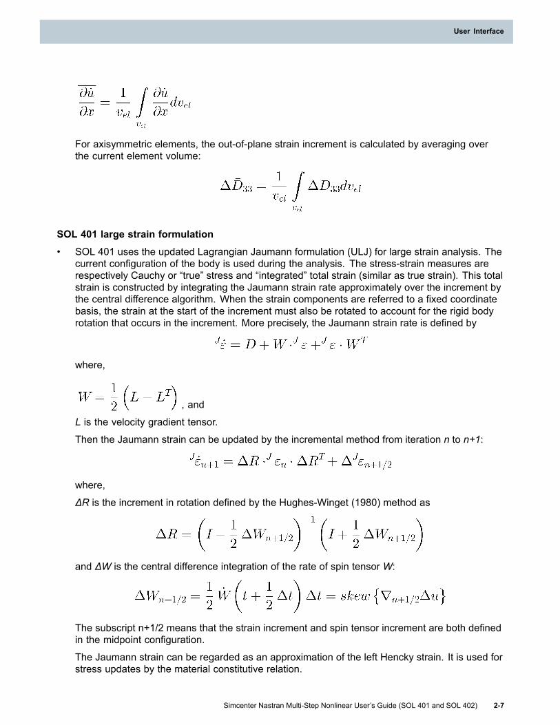
For axisymmetric elements, the out-of-plane strain increment is calculated by averaging overthe current element volume:
SOL 401 large strain formulation
• SOL 401 uses the updated Lagrangian Jaumann formulation (ULJ) for large strain analysis. Thecurrent configuration of the body is used during the analysis. The stress-strain measures arerespectively Cauchy or “true” stress and “integrated” total strain (similar as true strain). This totalstrain is constructed by integrating the Jaumann strain rate approximately over the increment bythe central difference algorithm. When the strain components are referred to a fixed coordinatebasis, the strain at the start of the increment must also be rotated to account for the rigid bodyrotation that occurs in the increment. More precisely, the Jaumann strain rate is defined by
where,
, and
L is the velocity gradient tensor.
Then the Jaumann strain can be updated by the incremental method from iteration n to n+1:
where,
ΔR is the increment in rotation defined by the Hughes-Winget (1980) method as
and ΔW is the central difference integration of the rate of spin tensor W:
The subscript n+1/2 means that the strain increment and spin tensor increment are both definedin the midpoint configuration.
The Jaumann strain can be regarded as an approximation of the left Hencky strain. It is used forstress updates by the material constitutive relation.
Simcenter Nastran Multi-Step Nonlinear User’s Guide (SOL 401 and SOL 402) 2-7
User Interface

Chapter 2: User Interface
• The time step size affects the Jaumann strain, so that finite time step sizes lead to an error in thecalculation of the Jaumann strain. For a uniaxial deformation, the Jaumann strain approachesthe logarithmic strain as the step size is reduced. For a rigid-body rotation, the Jaumann strainalso rotates, with the rotation of the Jaumann strain approaching the expected rotation as thestep size is reduced.
• The Jaumann strain method is the most frequently used strain rate. However, it is deficientwith large shear strain problems because it produces an artificial oscillation for a simple shearproblem. It can also be shown that the Jaumann strain is path-dependent in general, so that adeformation history in which the final deformations equal the initial deformations can produce(nonphysical) non-zero Jaumann strains, even in the limit of infinitesimally small time steps.
2.3 Nonlinear Effects in SOL 402Large displacement
The parameter LGDISP turns the nonlinear large displacement capability on/off. If you define theparameter LGDISP for SOL 402, you must include it in the bulk data portion of your input file. Thesingle PARAM,LGDISP setting is global and applies to all subcases.
• PARAM,LGDISP,-1 (default) - Large displacement effects are turned off for STATIC, PRELOAD,and DYNAMICS subcases.
For the MODES, CYCMODES, and FOURIER subcases, second-order effects are ignored.
As a consequence, BUCKLING subcases are not allowed.
Small strains are assumed and follow the Engineering strain law.
• PARAM,LGDISP,1 - Large displacement effects are turned on for STATIC, PRELOAD, andDYNAMICS subcases.
For the MODES, CYCMODES, and FOURIER subcases, second-order effects are taken intoaccount. In particular the stress stiffening effect of the previous static subcase.
For the BUCKLING subcases, nonlinear effects are split in two terms: a dead load part and avarying part. The varying part is related to the loads variation from its latest static equilibrium.
Large strain
The parameter LGSTRN turns on/off large strains, displacements, and rotations.
• PARAM,LGSTRN,0 (default) - Small strains are assumed.
• PARAM,LGSTRN,1 - Large strains, displacements, and rotations are assumed (that is, LGDISPis automatically set to 1). Large strain formulation is applicable to all elements.
In particular, nonlinear material laws will switch to a Cauchy stress and Logarithmic strain. AllTABLES1 stress/strain hardening curves should also use the same convention.
2-8 Simcenter Nastran Multi-Step Nonlinear User’s Guide (SOL 401 and SOL 402)
Chapter 2: User Interface

User Interface
Note
In SOL 402, LGDISP and LGSTRN both turn on large strains for all element types. Theonly difference between LGDISP and LGSTRN is that:
• if LGDISP=1, the {Biot (engineering) strain, Biot stress} stress-strain measure is usedby default.
• if you explicitly turn on large strains (LGSTRN=1), then the {log (True) strain, Cauchystress} stress-strain measure is used.
For more information, see Stress-strain measures (SOL 402) in the Multi-Step NonlinearUser's Guide.
2.4 Nonlinear Parameters in SOL 401: NLCNTL entryThe NLCNTL bulk entry can be used to define strategies for the incremental and iterative solutionprocesses. It is difficult to choose the optimal combination of all the options for a specific problem.However, based on a considerable number of numerical experiments, the default option was intendedto provide the best workable method for a general class of problems. You should start with thedefault settings.
The NLCNTL bulk entry defines the parameters for SOL 401 control. The NLCNTL=n case controlcommand selects the NLCNTL bulk entry, and can be defined in a subcase or globally. You can definethe parameters on the NLCNTL bulk entry using the following format.
1 2 3 4 5 6 7 8 9 10NLCNTL ID Param1 Value1 Param2 Value2 Param3 Value3
Param4 Value4 Param5 Value5 -etc-
For example,
NLCNTL 1 EPSU 1E-3 EPSP 1E-3 EPSW 1E-7 ++ CONV PW KSTEP 5 MAXITER 25
See the NLCNTL bulk entry in the Simcenter Nastran Quick Reference Guide for the list ofparameters and descriptions.
2.5 Nonlinear Parameters in SOL 402: NLCNTL2 entryThe NLNTL2 bulk entry defines all the solution control parameters for SOL 402. The parameters canvary from one subcase to another.
The NLCNTL=n case control command selects the NLCNTL2 bulk entry, and can be defined in asubcase or globally.
It is difficult to choose the optimal combination of all the NLCNTL2 bulk entry options for a specificproblem. However, the defaults were intended to provide the best workable method for a general
Simcenter Nastran Multi-Step Nonlinear User’s Guide (SOL 401 and SOL 402) 2-9
User Interface

Chapter 2: User Interface
class of problems. Therefore, if you have little insight or experience in a specific application, youshould start with the default values.
Analysis control
The NLCNTL2 bulk entry helps you to control the analysis itself. For instance, you can:
• Control the maximum displacement and/or rotation that you allowed in your model.
• Decide whether time-unassigned loads or temperatures are ramped or stepped.
• Take inertia into account in nonlinear dynamic subcases.
Plasticity and creep control options
In SOL 402, when the MATNL parameter is set to 1 (PARAM,MATNL,1) to turn creep and/or plasticityeffects on, you can turn these effects off at the subcase level with the CREEP and PLASTICTYparameters of the NLCNTL2 bulk entry. For more information, see Disable plasticity and creep.
Time integration
On the NLCNTL2 bulk entry, you select the one of the following integration schemes:
• Newmark implicit predictor-corrector scheme
• Hilber-Hughes-Taylor (HHT) implicit predictor-corrector scheme
• Generalized midpoint method
• Generalized-α method
It is difficult to recommend the optimal integration scheme because the number of nonlinear problemsis so large. However, studies show some behaviors that you can use as quick guidelines:
• The Generalized-α schema (θ=0.55) that is enabled by default is unconditionally stable. Thismethod remains stable even for large time steps and without loss of accuracy.
• The Newmark schema (β=1/4, γ=1/2) has no numerical damping. It converges reasonably whenthe time step is small enough. Newmark is unstable if γ < 1/2.
• The Hilber-Hughes-Taylor (α=0.05) shows moderate numerical damping and damps the highfrequencies, but without any loss of accuracy.
• The Generalized midpoint schema (θ=0.55) or the Newmark one (Newmark (β=0.5625,γ=1)) shows strong numerical damping characteristics, but damps both the lower and higherfrequencies. In general, this is an unwanted characteristic for an integration scheme exceptpossibly for special applications.
The Generalized midpoint schema, with θ=0.50, shows no numerical damping.
Equilibrium iteration and convergence
On the NLCNTL2 bulk entry, you can control the equilibrium iterations and the convergence of thesolve:
2-10 Simcenter Nastran Multi-Step Nonlinear User’s Guide (SOL 401 and SOL 402)
Chapter 2: User Interface

User Interface
• You can specify the maximum number of iterations that the automatic time stepping method hasto perform to complete a time step.
• You can specify force, displacement, and energy reference levels and tolerances used in theNewton-Raphson schema to stop the iteration process.
• While the Newton method is effective in most problems, in some specific problems, you can copewith difficulties in convergence due to the Newton method step length.
On the NLCNTL2 bulk entry, you can then activate the line search algorithm that will control thelength of the Newton method step by minimizing the energy error or the force residue.
Note
As the computing cost for each line search is comparable to that of an iteration, thepermanent activation of the line search can be counterproductive.
Automatic time stepping
On the NLCNTL2 bulk entry, you can:
• Choose between fixed time steps or automatic time stepping. You can also control the timestep size (minimum, maximum, increase ratio).
• Control the negative or zero pivots rejection.
• Control the viscous material integration.
Internal restart options
Internal restarts start a specified subcase with the computation state (displacements, velocities,stresses, state variables, and so on) of a preload, static, or dynamic subcase during the same solve.For example, you might want to start several non-sequentially dependent (NSD) subcases with theresults of a bolt preload subcase. Similarly, you can start other NSD subcases with the results ofa dynamics subcase.
You can use the RSUB parameter to select the subcase you want to restart from.
Note
This restart should not be confused with the external restart that starts a new run from acomputation state loaded from a previous solve. For more information on this restart,see SOL 402 Restart.
Contact options
On the NLCNTL2 bulk entry, you can define specific parameters for contact conditions, such as thecharacteristic length of the contact or the relaxation factor.
Simcenter Nastran Multi-Step Nonlinear User’s Guide (SOL 401 and SOL 402) 2-11
User Interface

Chapter 2: User Interface
Format
1 2 3 4 5 6 7 8 9 10NLCNTL2 ID PARAM1 VALUE1 PARAM2 VALUE2 PARAM3 VALUE3
PARAM4 VALUE4 PARAM5 VALUE5 -etc-
Example
SUBCASE 1LABEL = Subcase - Nonlinear Dynamics 1NLCNTL = 101TSTEP = 101ANALYSIS = DYNAMICSSEQDEP = YES
....NLCNTL2 101 AUTOTIM ON DTMAX0.010000 TETA0.600000 ++ TINTMTH MGENALP
For more information, see the NLCNTL2 bulk entry in the Simcenter Nastran Quick Reference Guide.
2.6 Iteration related output data (SOL 401)SOL 401 writes convergence data to the .f06 file. The following example demonstrates the format ofthis output.
The software might need to iterate at a time/solution point when searching for a solution thatsatisfies convergence. The output format includes the following numbering in the first two columns:
1. The first column is the accumulated number of iterations for the current subcase. This numberis reset to 1 at the start of a new subcase.
2. The second column is the iteration number for the current time/solution point. This number isreset to 1 at the start of a new time/solution point.
For example, if a subcase includes 4 time points, and the number of iterations for each time point is:
Time Point 1 has five iterations,Time Point 2 has three iterations,Time Point 3 has four iterations,Time Point 4 has three iterations,
2-12 Simcenter Nastran Multi-Step Nonlinear User’s Guide (SOL 401 and SOL 402)
Chapter 2: User Interface

User Interface
the numbers in the first columns would be as follows:
Accumulated numberof iterations
Current iterationnumber
Accumulated numberof iterations
Current iterationnumber
Time Point 1 Time Point 312345
12345
9101112
1234
Time Point 2 Time Point 4678
123
131415
123
You can define any combination of U, P, and W with the CONV parameter on the NLCNTL bulkentry to request which of displacement (U), force (P), and work (W) the software will consider forthe convergence criteria. By default, only work (W) is requested.
For each active convergence criteria, which is designated with the * next to the name in the output,the software includes the "n" or "y" next to the computed convergence value for that iteration, where"n" indicates that the specific criteria was not satisfied, and "y" indicates that it was satisfied.
Note: When you do not explicitly request load (P) as a criteria, the software still checks that theforce residual is reducing in size. The printed tolerance in this case is the force residual from thefirst iteration for the current solution/time point. As a result, the * will always appear next to theFORCE criteria in the output.
For the contact convergence data, there are three convergence tolerance columns. In addition,the software includes the "n" or "y" next to the computed convergence values for each iteration, where"n" indicates that the specific criteria was not satisfied, and "y" indicates that it was satisfied.
1. The first column depends on the contact convergence criteria you select with the CNTCONVparameter on the BCTPARM bulk entry:
- When CNTCONV=1 (default), the contact convergence criteria uses the penetration tolerance(PTOL parameter). In this case, the first column is labeled PENETR.- When CNTCONV=2, the contact convergence criteria uses the traction tolerance (CTOLparameter). In this case, the first column is labeled TRACTN.
2. The second column represents the contact force tolerance (RTOL parameter) and is labeledFORCE.
Simcenter Nastran Multi-Step Nonlinear User’s Guide (SOL 401 and SOL 402) 2-13
User Interface

Chapter 2: User Interface
3. The third column represents the contact damping tolerance (DCTOL parameter). It is labeledDAMP.
The CTDAMP parameter on the BCTPARM bulk entry is available to request the stabilizationdamping option when you are relying on the contact condition to prevent rigid body conditions,but the contact condition is not fully active.
The DCTOL parameter is available on the BCTPARM bulk entry to adjust the stabilizationdamping tolerance. When you request stabilization damping, the software will ramp the dampingtractions down as it iterates at a solution point until the following is satisfied.
where
λD are the damping tractions, and
λC are the contact tractions.
Note: In addition to the three contact convergence checks described above, if you did not request thedisplacement convergence criteria by including "U" with the CONV parameter on the NLCNTL bulkentry, the software also performs the following contact displacement convergence check.
where,
urel is the relative displacement of the nodes associated with a contact element, and
Δurel is the change in the relative displacement from the last converged solution/time point to thecurrent iteration.
The status of this check is included in the contact f06 output, which has the headings REL DISP,DUTOL, andWITHIN TOL. It is not represented in the three contact data columns described above. Itis possible for all three contact data columns to be satisfied and have a "y" in their respective column,yet the contact displacement convergence check has failed. If this occurs, the contact problem willnot be fully converged, and will result with an "n" in the CON column described below.
The software includes a column that summarizes the status for the solution convergence (EQUcolumn), the contact convergence (CON column), and the bolt preload convergence (BLT column).For example, when both contact and bolt preload are present in the solution, all three must have a "y"for the iteration to be considered converged.
Note: The bolt preload convergence column (BLT) is applicable only to bolts defined with ETYPE =1or ETYPE=3, and not to a bolt defined with ETYPE=2.
2-14 Simcenter Nastran Multi-Step Nonlinear User’s Guide (SOL 401 and SOL 402)
Chapter 2: User Interface

User Interface
2.7 Supported outputCase Control DescriptionACCELERATION Requests accelerations.
ADAPTERR Requests error estimates computed in a statics subcase (SOL 401only).
BCRESULTS Requests contact forces, tractions, separation distance, and the totaland incremental slide distances.
BGRESULTS Requests glue forces and tractions.
BOLTRESULTS Requests the bolt force and the axial strain output in a bolt preloadsubcase.
CKGAP Requests gap result output for chocking elements (SOL 401 only).CRSTRN Requests grid point creep strains on elements.CZRESULTS Requests results output for cohesive elements.DISPLACEMENT Requests displacement output.EKE Requests element kinetic energy output.ELAROUT Requests element add/remove status output (SOL 401 only).ELSTRN Requests elastic strain at grid points on elements.ELSUM Requests output of an element property summary.ESE Requests the output of the strain energy.FLXRESULTS Requests outputs for flexible sliders (SOL 402 only).FORCE Requests element force output.GCRSTRN Requests Gauss point creep strains on elements (SOL 401 only).GELSTRN Requests elastic strain at Gauss points (SOL 401 only).GPFORCE Requests grid point force balance output.
GPKE Requests kinetic energy at grid points in a modal subcase (SOL 401only).
GPLSTRN Requests Gauss point plastic strain output on elements (SOL 401only).
GSTRAIN Requests strain at Gauss points (SOL 401 only).
GSTRESS Requests stress at Gauss points (SOL 401 only).GTHSTRN Requests thermal strain at Gauss points (SOL 401 only).
HOUTPUT Requests the harmonics for results output in the cyclic and Fouriernormal modes subcase types.
JRESULTS Requests outputs for kinematic joints (SOL 402 only).JINTEG Requests output of the j-integral for crack analysis (SOL 401 only).MEFFMASS Requests modal effective mass output in a modal subcase.
MONVAR Selects degree-of-freedom for a displacement monitor plot (SOL 402only).
MPCFORCES Requests multipoint constraint force output.OLOAD Requests the form and type of applied load vector output.OMODES Requests selects a set of modes for output.
Simcenter Nastran Multi-Step Nonlinear User’s Guide (SOL 401 and SOL 402) 2-15
User Interface

Chapter 2: User Interface
OPRESS
For SOLs 401 and 402 including the Simcenter 3D Multiphysicsenvironment, requests output of the fluid penetrating pressure loaddefined with the PLOADFP bulk entry.
For the Simcenter 3D Multiphysics environment running SOL 401,requests the output of pressure computed by the Simcenter 3DThermal solver.
OSTNINI Requests initial strain output when an initial stress or strain is defined(SOL 401 only).
OTEMP Requests solution temperatures output on grid points.
PFRESULTS Requests progressive failure results output for composite solidelements.
PLSTRN Requests grid point plastic strain output on elements.
SET Defines a set of element or grid point numbers to be plotted (SOL402 only).
SETMC Sets definitions for modal, panel, and grid contribution results (SOL402 only).
SETMCNAME Specifies the title of a displacement monitor plot (SOL 402 only).SHELLTHK Requests shell thickness output (SOL 402 only).SPCFORCES Requests single-point force of constraint vector output.
STATVAR Requests state variable output computed by an external user definedmaterial routine.
STRAIN Requests element strain output.STRESS Requests element stress output.THSTRN Requests thermal strain at grid points on elements.VELOCITY Requests velocity at grid points.
2.8 Solver Support
Solver support for SOL 401
SOL 401 supports the sparse direct solver (default), the element iterative solver, the PARDISOsolver, and the MUMPS solver. To select the SOL 401 solver type, supply a pair of fields on theNLCNTL bulk entry of the form “SOLVER SPARSE”, “SOLVER ELEMITER”, “SOLVER PARDISO”, or“SOLVER MUMPS”.
You can request a different solver from one subcase to the next, but with the following exceptions.
• The dynamics subcase doesn’t support the element iterative solver. If the element iterative solveris requested for a dynamics subcase, it will revert to the sparse solver.
• The normal modes, cyclic modes, and Fourier modes subcases always use the sparse solver,and ignore the solver selection.
Additional information:
• The sparse direct solver is a robust and reliable option, well-suited to sparse models whereaccuracy is desired.
2-16 Simcenter Nastran Multi-Step Nonlinear User’s Guide (SOL 401 and SOL 402)
Chapter 2: User Interface

User Interface
• The element iterative solver performs well with solid element-dominated models. It may be afaster choice if lower accuracy is acceptable. You can optionally define the SMETHOD casecontrol command and the ITER bulk entry to alter any of the default options available on theITER entry.
• For problems involving contact and 3D solid elements, the element iterative solver is generallyfaster as compared to the sparse direct solver.
• The PARDISO solver is a hybrid direct-iterative solver, potentially faster with larger numbers ofcores than the sparse solver but with slightly lower accuracy.
Before Simcenter Nastran 2020.1, when you used the memory keyword to allocate memory forSimcenter Nastran, that allocation did not include memory for the Paradiso solver. Instead, theParadiso solver would use the available in-core memory that was not allocated to any application,including Simcenter Nastran.
Beginning with Simcenter Nastran 2020.1, Simcenter Nastran allocates a percentage of itsopen core memory to the Paradiso solver. By default, 75% of Simcenter Nastran's open corememory is allocated to the Paradiso solver. You can use the new system cell 734 to changethis percentage. For example, the system cell setting SYSTEM(734)=80 will request 80% ofSimcenter Nastran's available open core memory.
You can revert to the behavior before Simcenter Nastran 2020.1 by defining SYSTEM(735)=1.That is, when SYSTEM(735)=1 is defined, the Paradiso solver will use the available in-corememory that is not allocated to any application, including Simcenter Nastran.
Solver support for SOL 402
SOL 402 supports the sparse direct solver (the default) or the parallel solver. The element iterativesolver is not supported.
• On the NLCNTLG bulk entry, you can choose the Skyline, sparse, or parallel solver using theRESO parameter.
• For the parallel solver, SOL 402 supports distributed-memory parallel processing (DMP) andshared-memory parallel processing (SMP).
2.9 Parallel support
Parallel support for SOL 401
SOL 401 supports distributed-memory parallel processing (DMP) and shared-memory parallelprocessing (SMP).
• You can request shared-memory parallel processing using the PARALLEL or SMP) nastrankeyword. This keyword sets the number of MKL threads.
You can run Shared Memory Parallel (SMP) on a single machine with multiple processors andcores. It does not require a special license. If you are licensed to run a solution with the serialoption (that is, no parallel options), then you can run the same solution with SMP.
Simcenter Nastran Multi-Step Nonlinear User’s Guide (SOL 401 and SOL 402) 2-17
User Interface

Chapter 2: User Interface
SMP occurs for lower level operations such as matrix decomposition and matrix multiplication.Each SMP thread shares common memory and I/O. You request SMP by defining the number ofthreads with the parallel (or smp) keyword.
• You can request distributed-memory parallel processing using the DMP nastran keyword andnrec for RDMODES. This keyword sets the number of CPUs to use.
You can run DMP on a single machine with multiple processors, or multiple machines each withone or more processors communicating over a network.
The .f06 file will include a message similar to the following indicating the number of processorsused by the solution:
NUMBER OF PROCESSORS USED.....(NPROC) = n
The DMP methods divide the FE model into geometric and frequency parts to be solvedsimultaneously. Each process works on its own partition of the geometry or frequency range, ituses its own memory, and does I/O independently. You request DMP by defining the number ofprocesses with the following keywords:
DMP may be combined with SMP, so that each DMP process uses multiple SMP threads.
See Chapter 6 in the Simcenter Nastran Parallel Processing Guide for a description of the DMPmethods for each of the subcase types.
Parallel support for SOL 402
SOL 402 supports distributed-memory parallel processing (DMP) and shared-memory parallelprocessing (SMP).
• You can request shared-memory parallel processing using the PARALLEL or SMP) nastrankeyword. This keyword sets the number of MKL threads.
• You can request distributed-memory parallel processing using the MPI402 nastran keyword .This keyword sets the number of CPUs to use.
The .f06 file will include a message similar to the following indicating the number of processorsused by the solution:
NUMBER OF PROCESSORS USED.....(NPROC) = n
The DMP keyword provides no function in SOL 402.
Combining DMP and SMP processes in SOL 402
When combining DMP and SMP, each DMP process will spawn the number of threads as specifiedby the PARALLEL (or SMP) keyword.
Each DMP process will allocate its own memory, whereas the threads are sharing the same memorywithout any significant increase.
The total amount of memory specified by the memory keyword will be divided by two times thenumber of DMP processes because for each DMP process, the main executable and the MUMPSsolver used to solve the system of equations in parallel will both allocate the same amount of memory.
For best performances, you should:
2-18 Simcenter Nastran Multi-Step Nonlinear User’s Guide (SOL 401 and SOL 402)
Chapter 2: User Interface

User Interface
• Increase the total memory allocated by Nastran up to the machine’s memory if possible, unlessyou want to keep some available for other tasks.
• Choose the highest number of DMP processes that can fit in the total memory allocated byNastran.
• Ensure that each DMP process has enough memory for the given problem. If not, an errormessage will appear in the .f06 file that will give the amount of memory needed.
If the memory cannot be increased, the number of DMP processes must be decreased.
• Make sure that the number of DMP processes multiplied by the number of threads is at mostequal to the number of cores on the machine.
This is the case if all DMP processes are located on the same machine. If they are spreadover a cluster of machines, then you should ensure that the number of DMP processes oneach single machine multiplied by the number of threads is at most equal to the number ofcores on that machine
2.10 Subroutine to monitor solution progressThe external subroutine NUSOL is available for SOL 401, which you can use to monitor the status ofeach solution/time point. Simcenter Nastran sends the subroutine some basic solution/time pointinformation and status at the start and end of each solution/time point and subcase. You can usethe information provided to the subroutine, for example, to make a decision at each solution/timepoint whether to continue or stop the solution.
The source code for the subroutine is available for you to customize. A compiled version of thesubroutine is available for you to use with SOL 401. You can activate the subroutine with the systemcell setting SYSTEM(736)=2. When the subroutine is activated, you will see that the same data sentto the subroutine is also in the .f06 file. Each set of data will begin with the variable IRET. For example,
^^^^^^*************************************************************************************************^^^* STATICS SOLUTION *^^^* SUBCASE ID : 25 *^^^* SEQDEP : NO *^^^* SUBCASE START TIME : 0.000000E+00 *^^^* SUBCASE END TIME : 1.000000E+00 *^^^*************************************************************************************************^^^^^^
TEST FOR NUSOL, IRET 1TEST FOR NUSOL, SUBCASE_ID 25TEST FOR NUSOL, ANALYSIS_TYPE 1TEST FOR NUSOL, DTIME_BEGIN 0.200000000000000
^^^
• IRET has the following meanings:
=1 Beginning of the current subcase.
=2 Beginning of the current time step.
=3 End of the current time step.
Simcenter Nastran Multi-Step Nonlinear User’s Guide (SOL 401 and SOL 402) 2-19
User Interface
Chapter 2: User Interface
=-3 End of the current time step with error (no convergence)
=4 End of the current subcase
=5 End of the analysis.
• ANALYSIS_TYPE has the following meanings:
=1 Statics
=2 Dynamics
=3 Modal
=4 Preload
=5 Cycmodes
=6 Fourier
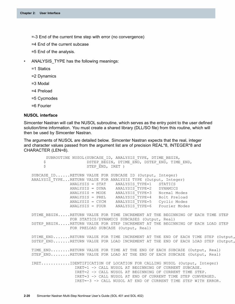
NUSOL interface
Simcenter Nastran will call the NUSOL subroutine, which serves as the entry point to the user definedsolution/time information. You must create a shared library (DLL/SO file) from this routine, which willthen be used by Simcenter Nastran.
The arguments of NUSOL are detailed below. Simcenter Nastran expects that the real, integerand character values passed from the argument list are of precision REAL*8, INTEGER*8 andCHARACTER (LEN=8).
SUBROUTINE NUSOL(SUBCASE_ID, ANALYSIS_TYPE, DTIME_BEGIN,$ DSTEP_BEGIN, DTIME_END, DSTEP_END, TIME_END,$ STEP_END, IRET )
SUBCASE_ID......RETURN VALUE FOR SUBCASE ID (Output, Integer)ANALYSIS_TYPE...RETURN VALUE FOR ANALYSIS TYPE (Output, Integer)
ANALYSIS = STAT ANALYSIS_TYPE=1 STATICSANALYSIS = DYNA ANALYSIS_TYPE=2 DYNAMICSANALYSIS = MODE ANALYSIS_TYPE=3 Normal ModesANALYSIS = PREL ANALYSIS_TYPE=4 Bolt PreloadANALYSIS = CYCM ANALYSIS_TYPE=5 Cyclic ModesANALYSIS = FOUR ANALYSIS_TYPE=6 Fourier Modes
DTIME_BEGIN.....RETURN VALUE FOR TIME INCREMENT AT THE BEGINNING OF EACH TIME STEPFOR STATICS/DYNAMICS SUBCASES (Output, Real)
DSTEP_BEGIN.....RETURN VALUE FOR STEP INCREMENT AT THE BEGINNING OF EACH LOAD STEPFOR PRELOAD SUBCASE (Output, Real)
DTIME_END.......RETURN VALUE FOR TIME INCREMENT AT THE END OF EACH TIME STEP (Output, Real)DSTEP_END.......RETURN VALUE FOR LOAD INCREMENT AT THE END OF EACH LOAD STEP (Output, Real)
TIME_END........RETURN VALUE FOR TIME AT THE END OF EACH SUBCASE (Output, Real)STEP_END........RETURN VALUE FOR LOAD AT THE END OF EACH SUBCASE (Output, Real)
IRET............IDENTIFICATION OF LOCATION FOR CALLING NUSOL (Output, Integer)IRET=1 -> CALL NUSOL AT BEGINNING OF CURRENT SUBCASE.IRET=2 -> CALL NUSOL AT BEGINNING OF CURRENT TIME STEP.IRET=3 -> CALL NUSOL AT END OF CURRENT TIME STEP CONVERGED.IRET=-3 -> CALL NUSOL AT END OF CURRENT TIME STEP WITH ERROR.
2-20 Simcenter Nastran Multi-Step Nonlinear User’s Guide (SOL 401 and SOL 402)
Chapter 2: User Interface

User Interface
IRET=4 -> CALL NUSOL AT END OF CURRENT SUBCASE.IRET=5 -> CALL NUSOL AT END OF THE ANALYSIS.
Build instructions
You can develop the external routine using FORTRAN or C, and compile for Windows or Linuxoperating systems.
Before you use NUSOL, you must build your own shared library to create a *.dll file on Windows or an.so file on Linux. Simcenter Nastran will link to this shared library for data exchange. You will need tohave the Fortran or C compiler to compile the corresponding source code.
Source code examples are included with the Simcenter Nastran installation at the following locations.
• Source code written in C can be found at:installation_location\scnas\usol\usolc\
• Source code written in FORTRAN can be found at:installation_location\scnas\usol\usolf\
Once your makefile is correctly defined and your compiler is configured, a shared library oflibusol.dll/libusol.so can be built. The table below lists the build commands and shared libraries forWindows and Linux.
Platform Build Command Shared LibraryWindows nmake libusol.dll libusol.dllLinux make libusol.so libusol.so
Demonstration models
Demonstration models are available in the Simcenter Nastran installation as shown below. Note thatall the models are integrated into a single library.
On Windows
Compiled Fortran code: installation_location\scnas\em64tntl\libusol_usolf.dll
Compiled C code: installation_location\scnas\em64tntl\libusol_usolc.dll
On Linux
Compiled Fortran code: installation_location\scnas\x86_64linuxl\libusol_usolf.so
Compiled C code: installation_location\scnas\x86_64linuxl\libusol_usolc.so
Simcenter Nastran Multi-Step Nonlinear User’s Guide (SOL 401 and SOL 402) 2-21
User Interface


Chapter 3: Subcase Types
3.1 Subcase analysis typeThe ANALYSIS case control command defines the subcase analysis type. SOL 401 and SOL 402allow any combination of the subcase types.
• Nonlinear static subcase: You include ANALYSIS=STATICS in a subcase.
• Nonlinear dynamic subcase (includes damping and inertia effects): You includeANALYSIS=DYNAMICS in a subcase.
• Bolt Preload subcase: You include ANALYSIS=PRELOAD in a subcase.
• Modal subcase: You include ANALYSIS=MODES in a subcase.
• Cyclic Normal Modes: You include ANALYSIS=CYCMODES in a subcase.
• Fourier Normal Modes: You include ANALYSIS=FOURIER in a subcase.
The ANALYSIS case control command does not have a default in SOL 401 or SOL 402. You mustdefine it in every subcase, and it cannot be defined globally.
The modal subcase should include the METHOD case control command which selects the EIGRLbulk entry. The EIGRL entry defines the data needed to perform the real eigenvalue analysis with theLanczos method. The modal subcase automatically includes the stress stiffening from the previousstatic subcase, and can potentially include follower stiffness and spin softening depending on the typeof loading in the previous static subcase. The NLCNTL bulk entry has parameter inputs which allowyou to control the stiffness contributions for the modal subcase.
Other subcase analysis type in SOL 402
SOL 402 allows the following additional subcase type.
Note that nonlinear buckling in SOL 401 is defined with the ANALYSIS=STATIC subcase type.See Nonlinear buckling (SOL 401).
• Buckling modes subcase (incremental stability): You include ANALYSIS=BUCKLING in asubcase.
ANALYSIS=BUCKLING must follow a ANALYSIS=STATICS.
For more information, see Linearized buckling (SOL 402).
3.2 Subcase sequencingYou can use the SEQDEP case control command to define any subcase type as sequentiallydependent (SD), or non-sequentially dependent (NSD).
Simcenter Nastran Multi-Step Nonlinear User’s Guide (SOL 401 and SOL 402) 3-1

Chapter 3: Subcase Types
Subcase sequencing in SOL 401
• SEQDEP=YES (default) – the subcase is an SD subcase.
SOL 401 uses time as the variable to increment temperatures and loads in a static subcase. AnSD static subcase uses the final time from the previous static subcase for its start time. Thestart time is used to compute the solution time steps in a static subcase. See Defining SolutionTime Steps (SOL 401).
An SD subcase can receive the final state variables from the previous static subcase. Forexample, plastic strains, creep strains, and displacements.
• SEQDEP=NO – the subcase is a NSD subcase.
An NSD subcase is independent. The start time for a static NSD subcase is 0.0. See DefiningSolution Time Steps (SOL 401).
An NSD subcase does not use any data from a previous subcase, regardless of the parametersettings on the NLCNTL bulk entry.
Subcase sequencing in SOL 402
SOL 402 uses time as the variable to increment loads. Both SD and NSD subcases in SOL 402 usethe final time from the previous subcase for their start time.
• SEQDEP=YES (default) - the subcase is an SD subcase.
An SD subcase uses the final computation state from the previous subcase for its starting state(for example, stress, strain, and displacements).
An SD subcase ignores the RSUB parameter on the NLCNTL2 bulk entry.
• SEQDEP=NO - the subcase is an NSD subcase.
By default, an NSD subcase does not use a previous computation state for its starting state.However, an NSD subcase can optionally reload the computation state from the end of anyprevious subcase using the RSUB=n parameter of the NLCNTL2 bulk entry, where n can be-1, 0, or >0:
-1 Same behavior as SEQDEP=YES.
0 Subcase does not use a computation state from a previous subcase for itsstarting state (default for SEQDEP=NO).
>0 Restart from the end of subcase n, where n references a previous subcasenumber.
In an ANALYSIS=PRELOAD subcase, the start time must be equal to the end time. ForANALYSIS=STATIC and DYNAMICS subcases, the end time must be greater than the start time.
An ANALYSIS=PRELOAD subcase can be defined after an ANALYSIS=STATIC or DYNAMICSsubcase. The ANALYSIS=PRELOAD subcase can only contain bolt forces and/or contact definitions.
For more information on defining times steps in SOL 402, see Defining solution time steps (SOL 402).
3-2 Simcenter Nastran Multi-Step Nonlinear User’s Guide (SOL 401 and SOL 402)
Chapter 3: Subcase Types

Subcase Types
3.3 Transient dynamic subcaseSolutions 401 and 402 support a transient dynamic subcase type to request a direct transient responseanalysis. You designate the transient dynamic subcase by including the ANALYSIS=DYNAMICScase control setting in the subcase.
A transient response analysis computes the behavior of a structure subjected to a time-varyingexcitation. The equation of motion for the dynamic subcase includes the stiffness, damping, and massterms with the option to output displacement, velocity, and acceleration at each degree-of-freedom.
Similar to the other subcase types, the transient dynamic subcase can optionally include geometrynonlinear effects when PARAM,LGDISP,1 is defined, and it can include the material nonlinear effectswhen plasticity, creep, and viscoelasticity are defined. A linear dynamic analysis occurs when nononlinear conditions are present.
You use the same inputs to define time assigned and time unassigned mechanical and thermalloads for dynamic and static subcases. The difference is that for the dynamic subcase, the softwareuses time explicitly.
Mass inputsIn the equation of motion for dynamic and modal subcases, the mass matrix is used in the inertia
force term . For the dynamic and static subcases, mass is also used to compute grid pointforces from the body loads such as gravity, angular velocity, and angular acceleration.
You can use the following inputs to define the mass properties:
• The mass matrix is automatically computed when mass density (ρ) is specified on the MATientries associated with the finite elements.
• Nonstructural mass per unit length can be defined on the PBAR and PBEAM entries. In addition,nonstructural mass per unit area can be defined on the PSHELL entries.
• The CONM1 entry allows you to input a fully coupled 6x6 mass matrix. You can also define halfof the terms on the CONM1 entry for a symmetric matrix.
• The CONM2 entry defines concentrated mass and inertia terms at a grid point.
• The CMASSi bulk entries can be used to define mass at a single degree-of-freedom (DOF) whenonly one DOF is referenced, or it can be used to define coupling between two DOF.
The following parameters are related to the specification of mass properties.
• PARAM,COUPMASS,1 – Requests that the coupled mass option be used rather than thelumped mass option for the elements that support the coupled mass option. By default, with thelumped mass option, the mass of an element is divided and distributed to the grid points. Withthe coupled mass option, the distributed mass is replaced by a non-diagonal mass matrix thatcouples the connected grid points. The coupled mass option is sometimes more accurate,but it uses more computation time.
Note that COUPMASS controls the type of mass matrix used for the inertia term in the dynamicequation of motion. Although, SOL 401 always computes body forces using the consistent massmatrix independent of the PARAM,COUPMASS specification.
Simcenter Nastran Multi-Step Nonlinear User’s Guide (SOL 401 and SOL 402) 3-3
Subcase Types

Chapter 3: Subcase Types
• PARAM,WTMASS,value – Specifies a factor by which to multiply the mass of the structure toobtain dimensionally correct mass. For example, if the ft-lb-sec system is used, and the massinput unit is pounds, then value = 1/32.174 = .031081. This factor operates on all mass terms.
Damping
All damping definitions for the transient subcase are applied to the viscous damping force term
in the equation of motion, where is the velocity, and is the total viscous dampingmatrix. The total viscous damping is the sum of three types of optional damping inputs:
where,
• is viscous damping explicitly defined with the CDAMPi, CVISC, CBUSH, or CBUSH1Dbulk entries.
• is damping proportional to the mass and stiffness matrices. The parameter ALPHA1 definesdamping proportional to the mass matrix, and the parameter ALPHA2 defines damping that is
proportional to the stiffness matrix. The proportional damping is computed as
• is structural damping, which is converted to viscous damping. For both SOLs 401 and 402,the GE field on the MATi entry defines the structural damping for the elements that referencethe material entry. For SOL 401 only, the parameter G defines a global structural damping,which is applied to the entire stiffness matrix.
For SOL 401, G and GE are converted to viscous damping using the parameters W3 and W4as follows.
Where:
G is the overall structural damping coefficient (PARAM,G).
W3 is a frequency in radians per unit time (PARAM,W3) for the conversion of the overall structuraldamping into viscous damping.
[K] is the global stiffness matrix.
GE is the element structural damping coefficient defined using the GE field on the material entries.
W4 is a frequency in radians per unit time (PARAM,W4) for the conversion of element structuraldamping into viscous damping.
[KE] is an element stiffness matrix.
For SOL 402, the parameters G, W3, and W4 are unsupported inputs, and W4 is internally set to1.0. As a result, for SOL 402, GE is converted to viscous damping as follows.
3-4 Simcenter Nastran Multi-Step Nonlinear User’s Guide (SOL 401 and SOL 402)
Chapter 3: Subcase Types

Subcase Types
Note that GE and G by themselves are dimensionless multipliers of the stiffness. Although,the viscous damping explicitly defined with the CDAMPi, CVISC, CBUSH, or CBUSH1D bulkentries have damping units.
Loads and constraints
The dynamic subcase supports the same loads and constraints as the static subcase. Specifically,both subcases support the definition of the LOAD and the DLOAD case control commands, whichreference time-unassigned and time-assigned loads, respectively. When the time unassigned loadsare defined, the parameter LVAR on the NLCNTL (SOL 401) or NLCNTL2 (SOL 402) bulk entries isavailable to optionally ramp the loads by the number of increments defined on the TSTEP1 bulk entry.
Time unassigned and time assigned temperature loads are also supported for both the dynamic andstatic subcases. The time unassigned temperature load is requested with the TEMP(LOAD) casecontrol command, and the time assigned temperature load is requested with the DTEMP case controlcommand. When the time unassigned temperature loads are defined, the parameter TVAR onthe NLCNTL (SOL 401) or NLCNTL2 (SOL 402) bulk entries is available to optionally ramp thetemperature loads by the number of increments defined on the TSTEP1 bulk entry.
You use the same inputs to define time assigned and time unassigned loads for dynamic and staticsubcases. The difference is that for the dynamic subcase, the software uses time explicitly.
Note that a time unassigned load is not specifically defined with a time function. Although, when youapply a time unassigned load and choose the ramp option, it behaves similar to a time assigned load.
See Loads in the Multi-Step Nonlinear User’s Guide.
Initial conditions
You can request initial displacement and velocity conditions for a dynamic subcase with the IC=ncase control command. The integer n on the IC case control references a TIC bulk entry. Only thePHYSICAL option (default) on the IC command is available, which is the option for defining initialconditions on grid points.
The IC command can be defined either in a dynamic subcase, or if all subcases includeANALYSIS=DYNAMICS, you can define the IC command above the subcase level (globally). Foreither definition, the software will only apply an initial condition to a dynamic subcase that is eitherthe first subcase, or if it is not the first, it must be non-sequentially dependent (SEQDEP=NO). Thesoftware ignores an initial condition when a dynamic subcase does not satisfy these rules, andinstead starts from the state of displacement, velocity, and acceleration from the previous preload,static, or dynamic subcase.
Subcase sequencing
The dynamic subcase can be combined with any of the other subcase types (STATICS, PRELOAD,MODES, CYCMODES, FOURIER). Below are some example scenarios.
Note that a sequentially dependent (SEQDEP=YES) modes subcase cannot follow a dynamicsubcase. Doing so will result in a fatal error.
Note that if you are incrementing time across sequentially dependent static and dynamic subcases,your time steps must continue from one subcase to next.
Simcenter Nastran Multi-Step Nonlinear User’s Guide (SOL 401 and SOL 402) 3-5
Subcase Types

Chapter 3: Subcase Types
• A non-sequentially dependent (SEQDEP=NO) dynamic subcase can be defined at any location inthe case control. For this case, the dynamic subcase begins from time=0.0, and with any initialvelocity or acceleration conditions you have defined for the model.
Example:
SUBCASE 1ANALYSIS=STATICSNLARCL=1....SUBCASE 2ANALYSIS=DYNAMICSSEQDEP=NO....
• A sequentially dependent (SEQDEP=YES) dynamic subcase can be defined at any location inthe case control. It can be defined before or after any of the other subcase types (STATICS,PRELOAD, MODES, CYCMODES, FOURIER) except for a static subcase, which requests anonlinear buckling analysis with the NLARCL=ID case control command. For all other cases, thedynamic subcase will start from the last converged configuration and state variables from the endof the prior static, preload, or dynamic subcase.
Example:
SUBCASE 1ANALYSIS=PRELOAD....SUBCASE 2ANALYSIS=STATICSSEQDEP=YES....SUBCASE 3ANALYSIS=DYNAMICSSEQDEP=YES....SUBCASE 4ANALYSIS=STATICSSEQDEP=YES....SUBCASE 5ANALYSIS=PRELOADSEQDEP=YES....SUBCASE 6ANALYSIS=DYNAMICSSEQDEP=YES....
• Any non-sequentially dependent (SEQDEP=NO) subcase type can follow a dynamic subcase.
Example:
SUBCASE 1ANALYSIS=DYNAMICS....SUBCASE 2
3-6 Simcenter Nastran Multi-Step Nonlinear User’s Guide (SOL 401 and SOL 402)
Chapter 3: Subcase Types

Subcase Types
ANALYSIS=STATICSSEQDEP=NO....SUBCASE 3ANALYSIS=DYNAMICSSEQDEP=YES....SUBCASE 4ANALYSIS=DYNAMICSSEQDEP=NO....
• A dynamic subcase can be included with a cyclic symmetry model. The cyclic symmetry requestis defined above the subcases (globally) and applies to all subcases. When either a static ordynamic subcase is included in a cyclic symmetry model, the solution is only performed forthe 0th harmonic.
Example:
CYCSET=100....SUBCASE 1ANALYSIS=STATICS....SUBCASE 2ANALYSIS=DYNAMICSSEQDEP=YES/NO....
Output summary
The dynamic subcase supports the same output requests as the static subcase. In addition, you canalso request velocity and acceleration for the dynamic subcase. All output for SOLs 401 and 402 is inSORT1 format, including the dynamic subcase. SORT2 output is not supported.
Time integration methods
Two types of analysis can be performed with the dynamic subcase:
• When the dynamic analysis includes the stiffness, damping, and inertia terms, the generalequation of motion is as follows.
• You can optionally turn the inertial effects off for a dynamic subcase by setting the parameterINERTIA=NO on the NLCNTL (SOL 401) or NLCNTL2 (SOL 402) bulk entries. The generalequation of motion for this analysis is as follows.
At each time step, a set of linear or nonlinear equations is solved. A full or modified Newton-Raphsonstrategy can be used.
Simcenter Nastran Multi-Step Nonlinear User’s Guide (SOL 401 and SOL 402) 3-7
Subcase Types

Chapter 3: Subcase Types
The TINTMTH parameter is available on the NLCNTL (SOL 401) or NLCNTL2 (SOL 402) bulk entriesto select the time integration method. In addition, the parameters; BETA, GAMA, ALFA, and TETAare available to define constant terms referenced in the following integration method descriptions.
• Newmark Method
Velocity is obtained from acceleration using a generalized single step integration operator as
Equation 3-1.
A similar integration operator is used to obtain displacement as
β and γ correspond to the parameters BETA and GAMA on the NLCNTL (SOL 401) or NLCNTL2(SOL 402) bulk entries.
o β= 1/4 and γ= 1/2 correspond to the assumption of average constant acceleration over thetime step. This set of values provides the Newmark unconditional scheme with maximumaccuracy.
o β= 1/6 and γ= 1/2 correspond to the assumption of linear acceleration over the time step.
Using a central difference operator for integrating velocity implies , so that we have
Equation 3-2.
From Equation 3-2, accelerations in terms of current displacements and state at t are derived as:
3-8 Simcenter Nastran Multi-Step Nonlinear User’s Guide (SOL 401 and SOL 402)
Chapter 3: Subcase Types

Subcase Types
Equation 3-3.
Then using Equation 3-1 and the chain rule, fc can be derived as . Likewise velocitiesin terms of current displacements and state at t are obtained as:
Equation 3-4.Note that the terms within square brackets in Equations 3-3 and 3-4 only depend ondisplacements, velocities and accelerations at t, and terms that contribute to the integrationoperator. Therefore, the former quantities should be stored as state variables (at nodes).
Finally the corresponding residual is computed as:
The residual and Jacobian for the Newmark operator are summarized in the following figure.
Figure 3-1. Newmark operator
Simcenter Nastran Multi-Step Nonlinear User’s Guide (SOL 401 and SOL 402) 3-9
Subcase Types

Chapter 3: Subcase Types
• Hilber-Hughes-Taylor (HHT) Method
The HHT integrator generalizes the Newmark operator, and in doing so, introduces a smallamount of numerical damping by weighting the residual between previous and current time step.This is done by modifying the (residual) equilibrium equations as
where α corresponds to the parameter ALFA parameter on the NLCNTL (SOL 401) or NLCNTL2(SOL 402) bulk entries.
Note that we can simply retain the definitions and most expressions from the Newmark operator,and summarize the HHT operator in the following figure.
Figure 3-2. HHT operator
This procedure includes numerical damping in the high frequency spectrum. This numericaldamping has a stabilizing effect on the time integration procedure while guaranteeing very goodaccuracy of integration of the low frequency range (including rigid body motion in particular).The particular value α= 0 generates zero numerical damping (and corresponds to the classicalNewmark scheme with β= 1/4 and γ = 1/2) while α= 1/3 generates maximum damping. It isgenerally recommended to use an intermediate value (α= 0.05 or α= 0.1).
• Generalized Alpha Method
The Generalized Alpha Method modifies the Hilber-Hughes-Taylor method by rewriting theequilibrium expression at time tn+1, then applying the time integration described with Newmark'smethod:
where θ corresponds to the parameter TETA parameter on the NLCNTL (SOL 401) or NLCNTL2(SOL 402) bulk entries.
The Newmark parameters are obtained by:
3-10 Simcenter Nastran Multi-Step Nonlinear User’s Guide (SOL 401 and SOL 402)
Chapter 3: Subcase Types

Subcase Types
This procedure allows to introduce some numerical damping in the high frequency spectrumof the system under consideration. This numerical damping has a stabilizing effect on thetime integration procedure while guaranteeing very good accuracy of integration of the lowfrequency range (including rigid body motion in particular). To obtain maximum damping inthe high frequencies and minimum damping in the low frequencies α and θ have to satisfy thefollowing relationship:
and θ has to satisfy .
• Modified Generalized Alpha Method
The Modified Generalized Alpha Method is obtained using a vector a of acceleration-like variablesin the Newmark integration formula.
Those additional variables are related to the accelerations by the following equation:
where,
are optimal algorithmic parameters for second-order ODEs.
This procedure allows to introduce some numerical damping in the high frequency spectrum ofthe system under consideration. This numerical damping has a stabilizing effect on the timeintegration procedure while guaranteeing very good accuracy of integration of the low frequencyrange (including rigid body motion in particular). Compare to Hilber-Hughes-Taylor method andGeneralized Alpha Method, this scheme enforces exactly equilibrium at every time step, whichguaranties second-order accuracy also for the accelerations and less sensitivity to variabletime steps
Damping is controlled by the spectral radius at infinity ρ∞: an undamped scheme is characterizedby ρ∞= 1, while ρ∞= 0 provides asymptotic annihilation of the high frequency response. TheRHOINF parameter on the NLCNTL bulk entry is available to define ρ∞.
Simcenter Nastran Multi-Step Nonlinear User’s Guide (SOL 401 and SOL 402) 3-11
Subcase Types
Chapter 3: Subcase Types
3.4 Cyclic symmetricThe cyclic solution method takes advantage of cyclic symmetry to reduce the time needed to createand solve a full 360 degree model. To use this method, you create a 3D-solid element model thatrepresents a fundamental segment. The fundamental segment represents a structure that is made upof N repetitions, where each repetition can be obtained by rotating the fundamental segment an anglethat is an integer multiple of 2π/N.
An important feature of this cyclic solution method is the automatic coupling of the translational DOFon the symmetry faces. The CYCSET case control command, which selects the CYCSET bulkentry, or multiple CYCSET entries with the CYCADD bulk entry, defines the coupling. The couplingdefinition is required and must be defined globally. As a result, the MPC equations created by thesoftware are applied in every subcase.
To define the coupling, you select the cyclic source and target regions on the CYCSET bulk entry. Avery useful feature of the coupling definition is that the mesh on the source and target regions canbe dissimilar. In addition, features such as holes in one or both of the symmetry faces are alsopermitted. The software internally computes the correct coupling conditions between the grids onthe source and target faces.
The CYCAXIS bulk entry is also required to define the default cylindrical coordinate system forthe coupling. The origin of this cylindrical system must be at the center of the revolution, and theZ-axis must be consistent with the axial direction.
Also see Cyclic Symmetry Theory.
CYCMODES subcase
A cyclic modes subcase is available and designated with ANALYSIS=CYCMODES in the subcase.The cyclic modes formulation includes the harmonic index, k, which represents an additionaldimension of the vector space that is not present in an "ordinary" modal analysis. For cyclic modelswith an even number of sectors (N is even), the allowable set of harmonics is 0,1, ...., N/2. For cyclicmodels with an odd number of sectors (N is odd), the allowable set of harmonics is 0,1,…, (N-1)/2.
You request the harmonic index values in which you want modes to be computed with theHARMONICS case control command, and a cyclic modal solution occurs for each harmonic indexindependently. For example, if you request 10 modes on the EIGRL bulk entry, and you request amodal solution for the 0th, the 1st, and the 2nd harmonic, a discrete cyclic modal solution occursfor each of these harmonics.
When computing the cyclic modes, the software uses a duplicate sector method. For harmonics k=0and k=N/2, there are distinct eigenvalues, and only one eigenvector component associated with eacheigenvalue. For all other harmonics (0 < k < N/2), each eigenvalue is repeated, and the displacement
vector for each corresponding eigenvalue has two components; the cosine component and the
sine component .
Static, bolt preload, and modal (non-cyclic modes) subcases
The static, bolt preload, and modal (non-cyclic modes) subcases can also be included in the input,and are designated with ANALYSIS=STATICS, ANALYSIS=PRELOAD, or ANALYSIS=MODALdefined in the subcase. These subcases use the MPC equations automatically created by thesoftware, but the displacements in the static and modal subcases are not cyclic. That is, thedisplacements only represent the 0th harmonic, n=1 fundamental sector.
3-12 Simcenter Nastran Multi-Step Nonlinear User’s Guide (SOL 401 and SOL 402)
Chapter 3: Subcase Types

Subcase Types
Any of the subcase types (statics, preload, modal and cyclic modes) can be defined as sequentiallydependent.
In SOL 401, you can define the parameters STRESSK, SPINK, and FOLLOWK on the NLCNTL bulkentry to request stress stiffening, spin softening, and follower stiffness, respectively.
Cyclic clocking and normalization for the CYCMODES subcase
As a result of the inherent symmetry with the cyclic modal solution, modes occur in pairs forharmonics 1 through N/2-1, where N is the total number of sectors.
Once Simcenter Nastran computes the normal modes, it uses the initially computed globaldisplacement vectors to do the following:
• The software clocks the eigenvector solution to the fundamental sector. This clocking ensuresthat, for the first mode in a mode pair, the maximum nodal displacement occurs on thefundamental sector.
• If you have selected either the AFNORM or DISP normalization options, the softwarerenormalizes using the maximum displacement relative to all sectors.
The clocking and normalization procedure is as follows.
The displacement result for a single mode and harmonic is represented by the equation:
The global displacement vectors and in a single mode are orthogonal to each other. In
addition, from one mode in a pair is related to from the same pair.
For a travelling wave with equal amplitude in any mode pair, every grid point traverses an ellipse inthree dimensional space. The maximum resultant displacement is the major axis of the ellipse. For agrid point i, the maximum resultant displacement is computed as follows.
is the cyclic cosine displacement vector (three components) at a specific grid point.
is the cyclic sine displacement vector (three components) at a specific grid point.
The software computes the following using the cyclic cosine and sine vectors:
The resultant displacement at each grid point i is computed as:
Simcenter Nastran Multi-Step Nonlinear User’s Guide (SOL 401 and SOL 402) 3-13
Subcase Types

Chapter 3: Subcase Types
The software determines the grid point with the maximum resultant displacement. For this grid pointii, the phase angle is computed as:
This phase angle will be used to clock the displacements to the fundamental sector.
The maximum displacement found at grid point ii is used to compute the normalization factor:
• For AF normalization, the factor is computed as:
where,
ω is the frequency for the mode, and
AFNORM is the parameter setting PARAM, AFNORM which defaults to 1.0.
For the modes considered as rigid body modes, the software sets ω = 1 when computing the AFnormalization factor. The software considers a mode to be a rigid body mode if its frequency isbelow the value of the parameter AFZERO (default=1.0 hz).
• For unit (MAX) normalization, the factor is computed as:
• For mass (MASS) normalization, the factor f=1.0 is used since the eigenvector was already massnormalized when the modes were computed initially.
The cyclic cosine and sine components are then clocked based on the computed values of .
The cyclic components for each mode are then reset to these values:
Cyclic modes subcase input summary• In SOL 401, the automatic coupling definition is required. The inputs for the coupling are
described under the ‘Automatic Coupling Details’ heading below.
• The ANALYSIS=CYCMODES case control command is defined in the specific subcases in whichyou are requesting the cyclic modes solution method.
• The HARMONICS case control command requests the specific harmonics in which modes arecomputed. "ALL" requests all possible harmonics. If you define the SID of a SET bulk entry,
3-14 Simcenter Nastran Multi-Step Nonlinear User’s Guide (SOL 401 and SOL 402)
Chapter 3: Subcase Types

Subcase Types
the SET entry lists the harmonic numbers to be computed, including "0" to request the zerothharmonic.
The maximum harmonic for a model is related to the total number of segments which wouldtheoretically exist to represent the full model.
o For an even total number of segments:
Maximum harmonic = Total number of segments/2.
For example, if a 30 degree segment is modeled, the total number of segments to create afull model is 360/30 = 12. Since 12 is even, the maximum harmonic = 12/2=6.
o For an odd total number of segments:
Maximum harmonic = (Total number of segments-1)/2.
For example, if a 40 degree segment is modeled, the total number of segments is 360/40= 9. Since 9 is odd, the maximum harmonic = (9-1)/2 = 4.
o As a result of the inherent symmetry in the cyclic modal solution, mode pairs exist forharmonic numbers 1 through N/2 -1. The software automatically outputs the mode pairsfor these subcase types for the modes requested with the EIGRL entry. For example, ifyou request 10 modes on the EIGRL entry:
For harmonic index 0 and N/2, 10 modes are computed.
For harmonic numbers 1 through N/2 -1, 20 modes are computed (10 distinct modes).
This behaviour is consistent for modes requested with the OMODES case control command.See the remarks on the OMODES command for details.
• The HOUTPUT case control command optionally requests the harmonics to output modes. "ALL"requests output for every harmonic requested on the HARMONICS command. You can definean integer to select the SID of a SET bulk entry, which lists the harmonic numbers to be output.These IDs are a subset of the IDs requested on the HARMONICS command. The C, S, C*, andS* describers on the HOUTPUT command are not supported by SOL 401 nor SOL 402.
• The METHOD case control command selects the EIGRL bulk entry which then defines theeigenvalue solution options. For example, the lower and upper frequency ranges and the numberof modes. Since a single EIGRL entry is selected in a subcase, the same EIGRL options areused when the software computes the modes for each harmonic.
Automatic coupling details (SOL 401)
• The symmetry faces are grouped into source and target regions. To do the automatic coupling,Simcenter Nastran internally rotates the target region grids into the source region grids, it doesa mesh refinement on both the source and target, and then creates MPC equations using thetarget as the dependent DOF and the source as the independent DOF. The MPC equations arecreated between any source and target region grids within the user defined search distance(SDISTi) using a weighted area method.
• The mesh on the source and target regions can be dissimilar. Features such as holes in one orboth of the symmetry faces are also permitted.
Simcenter Nastran Multi-Step Nonlinear User’s Guide (SOL 401 and SOL 402) 3-15
Subcase Types

Chapter 3: Subcase Types
• It is recommended that the source and target faces have similar geometry. If the source andtarget geometry is different, the software will still couple the appropriate source and target grids,although, the solution accuracy will be comprimised.
• You must define the automatic coupling globally. The resulting MPC equations are included inall subcases, including any static, preload, and modal (that is, a non-cyclic modes subcasewith ANALYSIS=MODAL).
Automatic coupling input summary (SOL 401)
• The CYCAXIS bulk entry is required to define the default cylindrical coordinate system for thecoupling. The origin of this cylindrical system must be at the center of the revolution, and theZ-axis must be consistent with the axial direction.
• The Z-axis of every cylindrical coordinate system referenced by the CYCSET entry must havethe same origin and direction as the z-axis of the default coordinate system selected with theCYCAXIS bulk entry.
• The displacement coordinate system of grid points which are defined on the rotation axis musthave a Cartesian displacement coordinate system. For all other grid points, a cylindricaldisplcement coordinate system is recommended. See Rules for source and target DOF.
• The CYCSET case control selects the CYCSET or CYCSADD bulk entries. The CYCSETcase control must be defined above the subcase level. As a result, the MPCs generated bythe automatic coupling are used in every subcase (cyclic modes, static, and "normal" normalmodes subcases).
• The BSURFS and BCPROPS bulk entries define the regions. These are existing inputs usedto define glue and contact regions.
• The CYCSET bulk entry pairs the source and target face regions.
o The source region selected in a pair must have a smaller positive theta location than thetarget region.
o The software will use the number of segments (NSEG) field to compute the angle betweenthe source and target faces. For example, if a 30 degree segment is modeled, NSEGwould be 12 = (360/30).
o The SDIST field is used to pair source and target grids when creating the MPC equations.From each source grid, the search occurs in both the positive and negative theta DOFdirections. If the SDIST field is undefined, the software will automatically compute the searchdistance. The software computed value is reported in the f06 file.
• The CYCADD bulk entry can optionally be used to combine multiple CYCSET bulk entries. Thevalue defined in the NSEG field on all CYCSET entries referenced by a CYCADD entry must bethe same. A fatal error will occur if any are inconsistent.
• The CYCFORCES case control command optionally requests the MPC force output for the gridswhich are included in the automatic coupling. It can be defined above the subcases (globally)or in a subcase.
3-16 Simcenter Nastran Multi-Step Nonlinear User’s Guide (SOL 401 and SOL 402)
Chapter 3: Subcase Types

Subcase Types
Rules for source and target DOF
• If you define SPC conditions on target region DOF with the SPC, SPC1, or SPCD entries, thesoftware reports a warning message that it is ignoring the SPC conditions on the target regionDOF, and the solution continues.
• If you include a target region DOF on an RBE2, RBAR, or RBE3 element as a dependent DOF,the software reports a warning message that it is ignoring the rigid connections on the targetregion DOF, and the solution continues.
• If you include a source or target region DOF on an MPC bulk entry as a dependent DOF, thesolution ends with a fatal error.
• Grid points which are defined on the Z-axis of the default cylindrical coordinate system must havea Cartesian displacement coordinate system. For the grid points which are defined on the Z-axisand are included in a source or target region, in addition to any conditions that you defined,Simcenter Nastran automatically applies the following SPC conditions during the solution.
o For the harmonic index k=0, Simcenter Nastran fixes DOF 1, 2.
o For the harmonic index k=1, Simcenter Nastran fixes DOF 3.
o For all other harmonic index values, Simcenter Nastran fixes all six DOF.
Post-processing the results
Simcenter Nastran outputs results for the fundamental sector. Due to the symmetric nature of theproblem and the orthogonal nature of the modes, the results for the entire structure (360 degreemodel) can be inferred from the results of the fundamental sector.
• For the 0th harmonic:
=
Where,
n = sector for which results are to be inferred.
= Results corresponding to the fundamental sector at harmonic 0.
results for sector n at harmonic 0.
• For harmonic k (0 < k < N/2),
Where,
N = Total number of sectors.
n = Sector for which results are to be inferred.
k = Harmonic index
Simcenter Nastran Multi-Step Nonlinear User’s Guide (SOL 401 and SOL 402) 3-17
Subcase Types

Chapter 3: Subcase Types
= Cosine cyclic component for the k harmonic of the mode being computed for thefundamental sector.
= Sine cyclic component for the k harmonic of the mode being computed for the fundamentalsector.
R = any output quantity of interest. For example, displacement or stress.
• For harmonic N/2:
Where,
n = Sector for which results are to be inferred.
= results corresponding to the fundamental sector at harmonic N/2.
= results for sector n at harmonic N/2.
3.5 Fourier harmonic solutionA Fourier normal modes subcase is available in SOL 401 and SOL 402 for models that includeaxisymmetric elements. The subcase is designated with the ANALYSIS=FOURIER andHARMONICS=N case control commands in the subcase.
The conventional axisymmetric element includes radial and axial degrees-of-freedom with novariation in theta.
In the Fourier normal modes subcase, the axisymmetric element has radial, axial and thetadegrees-of-freedom. In addition, the degrees-of-freedom are represented with harmonic terms of aFourier series of the form:
where,
c=cos(kθ) and s=sin(kθ),
k is the harmonic number,
are symmetric displacements, and
3-18 Simcenter Nastran Multi-Step Nonlinear User’s Guide (SOL 401 and SOL 402)
Chapter 3: Subcase Types

Subcase Types
are antisymmetric displacements.
Both symmetric and antisymmetric displacements are computed by Simcenter Nastran for a particularharmonic k.
With the Fourier normal modes subcase, you request which harmonic numbers a modal solutionshould occur, and the harmonic terms for modal output. For each harmonic number in whichyou request modes and output, the software can compute the symmetric and antisymmetricdisplacements, stress, strain, SPC force and grid point forces. You can use the typical case controlcommands to request the output. You can then optionally use the Simcenter post processor to displaythe physical results on either a 3D segment, or on a full 360 degree model display.
The modal solution for each harmonic term is discrete, and independent of other harmonic terms. Forexample, if you request 10 modes on the EIGRL bulk entry, and you request a modal solution forthe 0th, the 1st, and the 2nd harmonic term, a discrete modal solution will occur for each of theseharmonics. You will have 10 modes for the 0th, 10 modes for the 1st, and 10 modes for the 2nd term,and there is no coupling of the mode results between the different harmonics.
Static and modal (non-Fourier normal modes) subcases can also be included in the input, and aredesignated with the case control commands ANALYSIS=STATICS or ANALYSIS=MODAL. Although,the conventional axisymmetric element formulation is used in the static and modal subcases.
The Fourier normal modes subcase can optionally be sequentially dependent on a static subcase.
In SOL 401, you can optionally define the parameters STRESSK, SPINK, and FOLLOWK on theNLCNTL bulk entry to request the additional stiffness terms computed in the previous static subcase.
In addition to axisymmetric elements, the plane stress and the chocking elements can also beincluded with the Fourier normal modes subcase. In the Fourier normal modes subcase, gausslocations on the chocking element use the axisymmetric Fourier formulation if the location isconsidered chocked. That is, it includes stiffness in the radial, axial and theta degrees-of-freedom,and all degrees-of-freedom are represented using harmonic terms of a Fourier series. To beconsidered chocked, the loads in a previous static subcase should result in the chocked condition,and the consecutive Fourier normal modes subcase should be defined as sequentially dependent. Bydefault, all gauss locations on the chocking elements are considered unchocked in a Fourier normalmodes subcase, and use the plane stress element formulation.
For grid points which are defined on the rotation axis, in addition to any conditions that you defined,Simcenter Nastran automatically applies the following SPC and MPC conditions during the solution.
• For the harmonic index k=0, Simcenter Nastran fixes the radial (Ur) and azimuth (Uθ)degrees-of-freedom.
• For the harmonic index k=1, Simcenter Nastran fixes the axial degree-of-freedom, and it createsthe MPC condition Ur = Uθ for the cosine terms, and the MPC condition Ur = -Uθ for the sine terms.
• For the harmonic index k>1, Simcenter Nastran fixes all translational degrees-of-freedom.
Note:
Simcenter Nastran Multi-Step Nonlinear User’s Guide (SOL 401 and SOL 402) 3-19
Subcase Types

Chapter 3: Subcase Types
When axisymmetric elements are defined on the XZ-plane of the basic coordinate system, the X-axisof the basic system is the radial direction, the Z-axis of the basic system is the axial direction, andthe Y-axis of the basic system is the azimuth direction. The grid points defining these elementsmust have X ≥ 0.
When axisymmetric elements are defined on the XY-plane of the basic coordinate system, the Y-axisof the basic system is the radial direction, the X-axis of the basic system is the axial direction, andthe Z-axis of the basic system is the azimuth direction. The grid points defining these elementsmust have Y ≥ 0.
Fourier normal modes subcase input summary
• The ANALYSIS=FOURIER case control command should be defined in the subcase in which youare requesting the Fourier normal modes subcase in SOL 401.
• The HARMONICS case control command requests the specific harmonics in which modes willbe computed. The SET entry then lists the harmonic numbers to be computed, including "0" torequest the zeroth harmonic. Since there is an infinite number of harmonics in the Fourier normalmodes analysis, the describer "ALL" is not supported in the ANALYSIS= FOURIER subcase.
• The HOUTPUT case control command optionally requests the harmonics to output modes. "ALL"requests output for every harmonic requested on the HARMONICS command. An integer can bedefined to select the SID of a SET bulk entry listing the harmonic numbers to be output. TheseID's typically represent a subset of the ID's requested on the HARMONICS command. The C, S,C*, and S* describers on the HOUTPUT command are not supported by SOL 401.
• The METHOD case control command selects the EIGRL bulk entry, which then defines theeigenvalue solution options. For example, the lower and upper frequency ranges and the numberof modes.
3.6 Nonlinear buckling (SOL 401)A nonlinear buckling analysis is used to accurately determine what the critical buckling load is andhow a structure behaves after it has buckled. You can request a nonlinear buckling analysis in a SOL401 statics subcase. You can choose from one of the following three arc-length methods:
• Riks arc-length method
• Modified Riks arc-length method
• Crisfield arc-length method
To request the nonlinear buckling analysis, your statics subcase should include the standardANALYSIS=STATICS command along with the NLARCL=ID case control command. The ID on theNLARCL command selects the NLARCL bulk entry which defines the nonlinear buckling parameters.
The NLARCL command in the subcase is the trigger which the software uses to start the nonlinearbuckling analysis. The referenced NLARCL bulk entry is also required, even when the default valuesare used.
The nonlinear buckling statics subcase must be either the first subcase, or the last in a sequence ofstatic subcases. A nonlinear buckling statics subcase can only be followed by a modal subcase.
3-20 Simcenter Nastran Multi-Step Nonlinear User’s Guide (SOL 401 and SOL 402)
Chapter 3: Subcase Types

Subcase Types
• If the nonlinear buckling statics subcase is the first subcase, all of the loads defined in the currentsubcase are incrementally applied by the software during the arc-length solution.
• If the nonlinear buckling statics subcase is the last subcase and it is sequentially dependent, theloads applied in the previous subcase are held constant in the current subcase. The differencebetween the load defined in the nonlinear buckling statics subcase and the load from the previoussubcase is computed. This load difference is incrementally applied by the software during thearc-length solution.
You select loads in a nonlinear buckling statics subcase with either the LOAD=n or DLOAD=n casecontrol commands. Although, you cannot increment loads in a nonlinear buckling statics subcasewith a TSTEP1 bulk entry since the software increments the loads for you. If you define a TSTEP1entry in a nonlinear buckling statics subcase, you must define it with a constant time. That is, it musthave an end time (Tend) which is the same as the start time for that subcase. In addition, the outputfrequency option Nout on the TSTEP1 entry is ignored in a nonlinear buckling statics subcase. Theoutput frequency is instead controlled by the NOUTAL parameter on the NLARCL bulk entry.
If you want to define a specific load sequence up to the point of buckling, you can do this with staticsubcases without buckling defined before your nonlinear buckling statics subcase. In these previousstatic subcases, you can increment loads with the TSTEP1 bulk entry.
The NLARCL bulk entry has the following solution parameters:
TYPE
= RIKS selects the Riks arc-length method
= MRIKS selects the modified Riks arc-length method (Default)
= CRIS selects the Crisfield arc-length method
MINALR Minimum allowable arc-length adjustment ratio between increments for the adaptivearc-length method. (0.0<Real≤1.0; Default=0.25)
MAXALR Maximum allowable arc-length adjustment ratio between increments for the adaptivearc-length method. (Real>=1.0, Default=4.0)
MAXR Defines the overall upper and lower bounds on the load increment /arc-length inthe subcase.
SCALE Scale factor for controlling loading contribution in the arc-length constraint.(Real>0.0; Default = 0.0)
DESITER Desired number of iterations for convergence to be used for the adaptive arc-lengthadjustment. (Integer>0, Default=12)
MXINC Maximum number of controlled load increments done in the arc-length subcase(Integer>0; default=20)
LDFACIN Initial load factor. This load factor will be used to compute initial arc-length (REAL>0,DEFAULT=1.0).
NOUTAL
Skip factor for output of the incremental results. Output always occurs at the finalincrement. For example, if you define NOUTAL=2, output occurs at every otherconverged solution increment and for the final increment. If you define NOUTAL=0,output only occurs at the final increment. (Integer≥0; Default=1)
MXLDFAC Maximum value of load-factor at which solution will be terminated. (Real, Default =1.0)
Initial Imperfections
You define the X,Y,Z location of a grid point on the GRID entry. An option is available to adjust thislocation with a +/- delta X,Y,Z position. For example, if a grid point is defined on the GRID entry at
Simcenter Nastran Multi-Step Nonlinear User’s Guide (SOL 401 and SOL 402) 3-21
Subcase Types

Chapter 3: Subcase Types
1.0, 1.0, 0.0, and a delta of .2, 0.0, 0.0 is defined, the modeled location for this grid point becomes1.2, 1.0, 0.0. This location adjustment is useful in the nonlinear buckling analysis to define animperfection. For example, an imperfection on the side of a cylinder which is under axial compressionwill impose a deliberate location for buckling.
The grid point imperfections are selected with the IMPERF case control command which selects theIMPERF or IMPRADD bulk entries. The IMPRADD entry allows you to combine multiple IMPERFentries, and scale the referenced imperfection sets either independently or collectively.
The IMPERF case control command must be defined globally (above the subcases). As a result, theupdated location of the referenced grid points applies to all subcases.
Restrictions
• The software issues a fatal error if LGDISP=-1 and an arc-length solution is requested.
• The software issues a fatal error if an arc-length solution is requested in the context of aSimcenter 3D Multiphysics solution.
• The software issues a fatal error if a sequentially dependent STATICS or PRELOAD subcasefollows an arc-length subcase.
• The software issues a fatal error if a sequentially dependent arc-length subcase follows anothersequentially dependent arc-length subcase.
• An enforced displacement defined with the SPCD bulk entry is held constant in a nonlinearbuckling solution.
Arc-length theory
The concept of the arc-length method is to modulate the applied loads in order to produce solutionswith displacement increments of manageable size of a given load step. In order to modulate theapplied load, an additional variable, the load factor, and a constraint equation are introduced. Thereare various approaches to providing a constraint equation.
Consider a residual load {R}.
Equation 3-5.
where F represents the internal forces, and the total external load P is expressed as:
Equation 3-6.
where P0 denotes the applied load at the end of the preceding subcase, ΔP represents the loadincrement in the current subcase, and μ is the load factor varying from 0 to 1, but not limited to thisrange, within the subcase. Linearizing {R} about (u,μ), R(u,μ) can be expressed as:
3-22 Simcenter Nastran Multi-Step Nonlinear User’s Guide (SOL 401 and SOL 402)
Chapter 3: Subcase Types
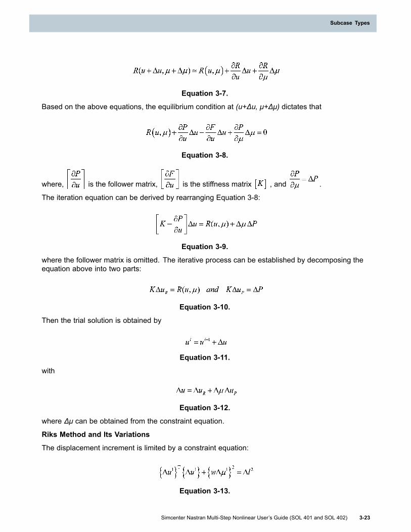
Subcase Types
Equation 3-7.
Based on the above equations, the equilibrium condition at (u+Δu, μ+Δμ) dictates that
Equation 3-8.
where, is the follower matrix, is the stiffness matrix , and .
The iteration equation can be derived by rearranging Equation 3-8:
Equation 3-9.
where the follower matrix is omitted. The iterative process can be established by decomposing theequation above into two parts:
Equation 3-10.
Then the trial solution is obtained by
Equation 3-11.
with
Equation 3-12.
where Δμ can be obtained from the constraint equation.
Riks Method and Its Variations
The displacement increment is limited by a constraint equation:
Equation 3-13.
Simcenter Nastran Multi-Step Nonlinear User’s Guide (SOL 401 and SOL 402) 3-23
Subcase Types
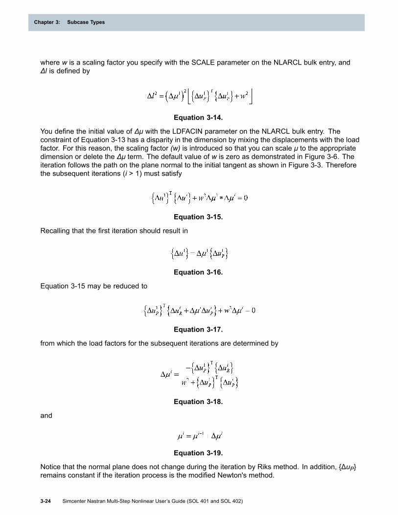
Chapter 3: Subcase Types
where w is a scaling factor you specify with the SCALE parameter on the NLARCL bulk entry, andΔl is defined by
Equation 3-14.
You define the initial value of Δμ with the LDFACIN parameter on the NLARCL bulk entry. Theconstraint of Equation 3-13 has a disparity in the dimension by mixing the displacements with the loadfactor. For this reason, the scaling factor (w) is introduced so that you can scale μ to the appropriatedimension or delete the Δμ term. The default value of w is zero as demonstrated in Figure 3-6. Theiteration follows the path on the plane normal to the initial tangent as shown in Figure 3-3. Thereforethe subsequent iterations (i > 1) must satisfy
Equation 3-15.
Recalling that the first iteration should result in
Equation 3-16.
Equation 3-15 may be reduced to
Equation 3-17.
from which the load factors for the subsequent iterations are determined by
Equation 3-18.
and
Equation 3-19.
Notice that the normal plane does not change during the iteration by Riks method. In addition, {ΔuP}remains constant if the iteration process is the modified Newton's method.
3-24 Simcenter Nastran Multi-Step Nonlinear User’s Guide (SOL 401 and SOL 402)
Chapter 3: Subcase Types

Subcase Types
Alternatively, the normal plane may be updated at every iteration. If the normal plane is to be normalto the cumulative incremental displacements for the preceding iterations as shown in Figure 3-4, theorthogonality condition in Equation 3-15 should be modified to:
Equation 3-20.
The increment in the load factor for i > 1 is obtained by solving Equation 3-20,
Equation 3-21.
This variation of Riks method has an advantage over the Crisfield method as it avoids the solution ofa quadratic equation.
Crisfield Method
Instead of iterating on the normal plane, the solution is sought on the surface defined by Equation3-13 with an arc-length of Δl as depicted in Figure 3-5,
Equation 3-22.
This constraint can be interpreted as keeping the incremental displacement constant, if w=0, asshown in Figure 3-6. Substituting Equation 3-12 into the preceding equation, we obtain a quadraticequation in terms of Δμ:
Equation 3-23.
where
Equation 3-24.
Since the Crisfield method leads to a quadratic equation, the selection of the proper root of thisequation becomes the most critical process for the success of this method. There are two roots toEquation 3-23,
Simcenter Nastran Multi-Step Nonlinear User’s Guide (SOL 401 and SOL 402) 3-25
Subcase Types

Chapter 3: Subcase Types
Equation 3-25.
The root is chosen so that the angle between two vectors {ui-1 - uo} and {ui - uo} is less than 90degrees,
Equation 3-26.
There are cases where no roots can be found. Such is the case when the trial solution is far from thetrue solution and stays outside the region covered by the arc-length. In this case, the trial solutionvector is scaled so that the direction vector intersects with the surface defined by Equation 3-22.
The wrong choice of the root could cause an unintentional loading path reversal, by which the solutionreturns to the previous state. Such cases can be detected by checking the orthogonality of theincremental displacements of the two successive solutions. If this case is detected, the root is chosenso that the angle between {ui - uo} and {ui - uo} is an acute angle.
Adaptive Arc-Length Method
It is difficult to estimate a proper arc-length for multi-degree-of-freedom problems. The initialarc-length for the Crisfield method can be determined by
Equation 3-27.
with
Δμ1 = μ1 = LDFACIN parameter on the NLARCL bulk entry.
You can define the maximum number of increments in the subcase with the MXINC parameteron the NLARCL bulk entry.
The arc-length should be continuously updated at every increment using the information gatheredduring the preceding increment. One method is to reduce the arc-length if it requires an excessivenumber of iterations to attain a converged solution,
Equation 3-28.
3-26 Simcenter Nastran Multi-Step Nonlinear User’s Guide (SOL 401 and SOL 402)
Chapter 3: Subcase Types

Subcase Types
where Id is the desired number of iterations for convergence and defined with the DESITERparameter on the NLARCL bulk entry, and Imax is the number of iterations required for convergencefrom the preceding step.
The adaptive process should be based on the arc-length ratio,
Equation 3-29.
Combining two criteria, the new arc-length ratio is adapted to the nonlinearity by
Equation 3-30.
In order to maintain the stability for the adaptive process, ALRATIO should also be bounded,
MINALR < ALRATIO < MAXALR
You can define the parameters MINALR and MAXALR on the NLARCL bulk entry, which have thedefaults of 0.25 and 4., respectively. If the adjusted ALRATIO falls outside the bounds, ALRATIOis reset to the limit. Then the arc-length is updated at the beginning of the next step based onALRATIO as follows:
Δlnew = ALRATIO * Δlold
In the unstable regime where the stiffness is negative, the load factor decreases with a forward step.When this happens, the sign of Δμ1 should be reversed. This possibility should be examined at thebeginning of each increment. The sign can be determined by the sign of a dot product,
Equation 3-31.
An adaptive bisection algorithm is also incorporated to cope with divergent cases. If the iterativeprocess using the arc-length method tends to diverge, the arc-length is bisected. The bisection iscombined in concert with the stiffness matrix update strategy. The bisection procedure continuesuntil the iterative process is stabilized and a converged solution is found. However, the number ofcontiguous bisections is limited by the parameter MAXBIS on the NLCNTL bulk entry. The variablearc-length at every increment invokes the recovery from the bisection process once the difficulties inconvergence are overcome.
Simcenter Nastran Multi-Step Nonlinear User’s Guide (SOL 401 and SOL 402) 3-27
Subcase Types

Chapter 3: Subcase Types
Figure 3-3. Riks Method
Figure 3-4. Modified Riks Method
3-28 Simcenter Nastran Multi-Step Nonlinear User’s Guide (SOL 401 and SOL 402)
Chapter 3: Subcase Types

Subcase Types
Figure 3-5. Crisfield Method - Arc-length in terms of Combined Variables
Figure 3-6. Crisfield Method - Arc-length in terms of Displacements
3.7 Linearized buckling (SOL 402)The non-linear behavior of a slender structure can be complex: you can encounter limit points wherethe load vs displacement curves reach a maximum or a bifurcation point where the structure bucklesfrom one mode shape to another mode (orthogonal to the primary one).
To better understand the behavior, you can calculate critical loads and buckling modes by solving thestability eigenvalue problem.
Simcenter Nastran Multi-Step Nonlinear User’s Guide (SOL 401 and SOL 402) 3-29
Subcase Types

Chapter 3: Subcase Types
Stability eigenvalue problem
In the neighborhood of an equilibrium point, the tangent stiffness matrix can be developed in functionof the load factor:
KT = K*T + Δλ * K'T + Δλ2 * K''T.
For structural elements, if a total Lagrangian formulation and Green strains are used, and if thematerial is elastic, this development is correct. Otherwise, it is only an approximation.
A linearization of this stiffness matrix is performed and the following eigenvalue problem is solved:
(K*T + Δλ * K'T)q = 0.
In order to compute the 1st derivative K'T, the following procedure is used:
1. The solver computes a variation of displacements from the variation of the external forces bysolving the equation:
K*T * Δq = ΔF.
2. Then, the solver computes the tangent stiffness matrix at two different points:
K1T = KT (q + Δq).
K2T = KT (q + 2Δq).
3. The 1st derivative K'T is then solved as a combination of the 3 matrices:
K'T = 0.5 * (4K1T - K2T - 3K*T).
For structural elements in total Lagrangian formulation with elastic material, this method gives thetrue geometric stiffness: the critical buckling load will not depend on the size of Δλ.
In case of non-linear material (plastic or other), the tangent constitutive law is kept constant in the 3computations of the stiffness matrix.
Workflow
1. After at least one ANALYSIS=STATICS subcase n, you define a ANALYSIS=BUCKLING subcasen+1.
Note
ANALYSIS=BUCKLING must follow a ANALYSIS=STATICS, not aANALYSIS=DYNAMICS.
2. The buckling subcase uses the last equilibrium state of the previous subcase n to computetangent stiffness matrix K*T.
3. The variation of the load (ΔF) is computed according to the loading time dependent function andfor a variation of time of 1 sec after the final time of subcase n.
4. The loads in the model that do not vary in between the time interval [tn, tn + 1 sec] are consideredas dead loads: they are applied on the structure but are not involved in the buckling process (Fn).
3-30 Simcenter Nastran Multi-Step Nonlinear User’s Guide (SOL 401 and SOL 402)
Chapter 3: Subcase Types

Subcase Types
The loads in the model that vary in between the time interval [tn, tn + 1 sec] are considered asworking loads: these are the loads that are involved in the buckling process (ΔF).
5. If λ is the buckling factor given by modal analysis, the critical loading is:
Fcrit = Fn + λΔF.
Note
You can repeat the sequence of STATICS subcase followed by BUCKLING subcaseseveral times.
Result analysis and assumptions
• If contact conditions are defined, the contact configuration is supposed to be constant during themodal analysis. Closed contact will be kept closed and open contact will be kept open. As far asa buckling mode amplitude is unknown, penetration could be observed in post processing.
• If some enforced displacements (SPCD) exist, they are considered fixed in the buckling modeanalysis.
• The buckling factor λ gives you the proportion of load variation that must be applied to maketangent matrix singular.
The behavior is supposed to be locally linear, displacements and stress are supposed to beproportional to a constant variation: q(λ) = qn + λΔq and σ(λ) = σn + λΔσ.
o If λ is > 0: the maximum load or the bifurcation point is not yet reached. In case of bifurcation,the post buckling behavior will probably looks like the buckling mode. It can eventually beused to introduce an imperfection in the structure.
o If λ is < 0: the maximum load or the bifurcation point has already be reached. The non-linearcomputation has probably shown negative pivots and the equilibrium can be unstable. In thiscase, you can use RJPN parameter of the NLCNTL2 bulk entry to reject unstable time step.
Example
Case Control
NASTRAN SYSTEM(674)=1$SOL 402CEND$*$*$$$$$$$$$$$$$$$$$$$$$$$$$$$$$$$$$$$$*$* CASE CONTROL$*$*$$$$$$$$$$$$$$$$$$$$$$$$$$$$$$$$$$$$*TITLE = Buckling analyses of a compressed plateSUBTITLE = Several load levelsECHO = UNSORT
Simcenter Nastran Multi-Step Nonlinear User’s Guide (SOL 401 and SOL 402) 3-31
Subcase Types

Chapter 3: Subcase Types
SPC = 1DLOAD = 2METHOD = 10DISPLACEMENT(PRINT) = ALLSTRESS(PRINT) = ALL$SUBCASE 1ANALYSIS = STATICSLABEL = First Loading [0-1]TSTEP = 101$SUBCASE 2ANALYSIS = BUCKLINGLABEL = Buckling analysis with unitary loadMETHOD = 20SEQDEP = YESEKE(PRINT,THRESH=0.3) = ALL$SUBCASE 3ANALYSIS = STATICSLABEL = Loading up to 100. [1-100]TSTEP = 102$SUBCASE 4ANALYSIS = BUCKLINGLABEL = Buckling analysis at 100 loadMETHOD = 40SEQDEP = YESEKE(PRINT,THRESH=0.3) = ALL$SUBCASE 5ANALYSIS = STATICSLABEL = Loading up to 250. [100-250]TSTEP = 103
Time steps definition
TSTEP1 101 0.01 1 ENDTSTEP1 102 1.0 1 ENDTSTEP1 103 2.5 1 END
Eigenvalues selection
$------1-------2-------3-------4-------5-------6-------7-------8-------9------10$EIGRL SID V1 V2 ND MSGLVL MAXSET SHFSCL NORMEIGRL 20 0. 500. 50 MAXEIGRL 40 5 1
Loads
$$ Loading
3-32 Simcenter Nastran Multi-Step Nonlinear User’s Guide (SOL 401 and SOL 402)
Chapter 3: Subcase Types
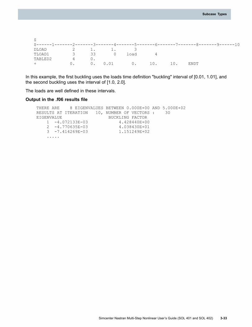
Subcase Types
$$------1-------2-------3-------4-------5-------6-------7-------8-------9------10DLOAD 2 1. 1. 3TLOAD1 3 33 0 load 4TABLED2 4 0.+ 0. 0. 0.01 0. 10. 10. ENDT
In this example, the first buckling uses the loads time definition "buckling" interval of [0.01, 1.01], andthe second buckling uses the interval of [1.0, 2.0].
The loads are well defined in these intervals.
Output in the .f06 results file
THERE ARE 8 EIGENVALUES BETWEEN 0.000E+00 AND 5.000E+02RESULTS AT ITERATION 10, NUMBER OF VECTORS : 30EIGENVALUE BUCKLING FACTOR
1 -4.072133E-03 4.428440E+002 -4.770635E-03 4.038430E+013 -7.414269E-03 1.151249E+02.....
Simcenter Nastran Multi-Step Nonlinear User’s Guide (SOL 401 and SOL 402) 3-33
Subcase Types


Chapter 4: Element support
4.1 Element OverviewThe following summarizes all of the elements and materials supported in SOLs 401 and 402.
• The 3D solids elements CTETRA, CHEXA, CPENTA and CPYRAM are supported for linear,geometric nonlinear, and material nonlinear analysis.
• The axisymmetric elements CQUADX4, CQUADX8, CTRAX3, CTRAX6, the plane strainelements CPLSTN3, CPLSTN4, CPLSTN6, CPLSTN8, and the plane stress elements CPLSTS3,CPLSTS4, CPLSTS6, CPLSTS8 are supported for linear, geometric nonlinear, and materialnonlinear analysis.
The grid points on these elements must all lie in either the XZ plane, or all in the XY plane of thebasic coordinate system. The software automatically determines the orientation.
When axisymmetric elements are defined on the XZ plane, X is the radial direction, and Z is theaxial direction. The grid points defining these elements must have X ≥ 0.
When axisymmetric elements are defined on the XY plane, Y is the radial direction, and X is theaxial direction. The grid points defining these elements must have Y ≥ 0.
• In SOL 401, a special, generalized plane strain formulation is available using the CPLSTN3,CPLSTN4, CPLSTN6, and CPLSTN8 element types. See Generalized plane strain analysis.
• In SOL 401, the chocking element is available. A chocking element is a special type ofaxisymmetric element used to model regions in an axisymmetric analysis that can carry acompressive hoop stress, but cannot carry a tensile hoop stress. See Chocking elements.
• The cohesive element is available to model adhesively bonded interfaces. Cohesive elements canaccount for compliance in the connection and damage in the material. See Cohesive elements.
• The bar and beam elements defined with the CBAR and CBEAM entries are available. Theysupport large displacements and rotations when large displacements are requested withPARAM,LGDISP,1 in SOL 401 or PARAM,LGSTRN,1 in SOL 402.
In SOL 402, nonlinear behaviors of bar and beam elements are only available for thin sections.
• The shell elements CTRIAR, CQUADR, CTRIA6, and CQUAD8 entries are supported. CQUAD4and CTRIA3 elements are also supported as inputs and the software will treat them as CQUADRand CTRIAR elements.
• The spring elements CELAS1, CELAS2, CBUSH1D, and CBUSH are supported.
• The RBE2 and RBAR rigid elements are supported with optional large displacement effects andthermal expansion. The RBE3 rigid element is also supported, but in SOL 401, it does not supportlarge displacement effects or thermal expansion. In SOL 402, it supports large displacements,rotations, and thermal expansion . See Rigid element support.
Simcenter Nastran Multi-Step Nonlinear User’s Guide (SOL 401 and SOL 402) 4-1

Chapter 4: Element support
• The mass elements CMASSi and CONMi are supported.
• The PSOLID or the PCOMPS bulk entries define the element properties. The PCOMPS isoptionally used to define a layered solid composite property.
You can model progressive ply failure in solid composites. See Progressive failure analysisin solid composites.
• The supported material types include the following.
The MAT1 and MATT1 (temperature dependent) bulk entries define isotropic materials.
The MAT3 and MATT3 (temperature dependent) bulk entries define isotropic materials.
The MAT9 and MATT9 (temperature dependent) bulk entries define anisotropic materials.
The MAT11 and MATT11 (temperature dependent) bulk entries define orthotropic materials.
The MATDMG bulk entry defines material properties for progressive ply failure.
In SOL 402:
The MATHE bulk entry defines Hyperfoam or Mooney-Rivlin hyperelastic materials.
The MATHEM or MATHP bulk entries define the Ogden hyperelastic material.
The MATHEV bulk entry adds viscoelastic properties.
Plastic and creep materials can optionally be assigned to the 3D solid elements, axisymmetricelements, the plane stress elements, and the plane strain elements. You can enable one or bothplasticity/creep in all subcases, or in specific subcases. See Support for plasticity analysis andSupport for creep analysis.
Externally computed, user defined material models are supported. You can define a materialmodel by developing and compiling an external routine. See User defined materials.
• You can request stress norm, stress error norm, strain energy norm, and strain energy errornorm output. The output is computed and stored on an individual element basis. The Pre/Postapplication uses the output for adaptive meshing. See Error estimator for mesh refinement.
• In SOL 401, you can compute and output the j-integral in a crack simulation. The j-integral outputcan be requested and used by third-party software like Zencrack to perform a fracture mechanicsanalysis. The CHEXA bulk entry allows for a collapsed element definition. See Crack simulation.
• In SOL 402, you can define kinematic joints. See Kinematics joints.
4.2 Elements in nonlinear analysisIn nonlinear finite element analysis, lower-order elements are often preferred over higher-order onesbecause of their robustness and reasonable accuracy at reduced costs. The software supports linearelements, rather than quadratic or cubic elements, to process nonlinearity. When using lower-orderelements, quadrilateral and hexahedral elements are generally preferred over triangular, pentahedralor tetrahedral elements. Triangular and tetrahedral elements can exhibit excessively stiff behavior,and caution is needed when using these elements.
4-2 Simcenter Nastran Multi-Step Nonlinear User’s Guide (SOL 401 and SOL 402)
Chapter 4: Element support
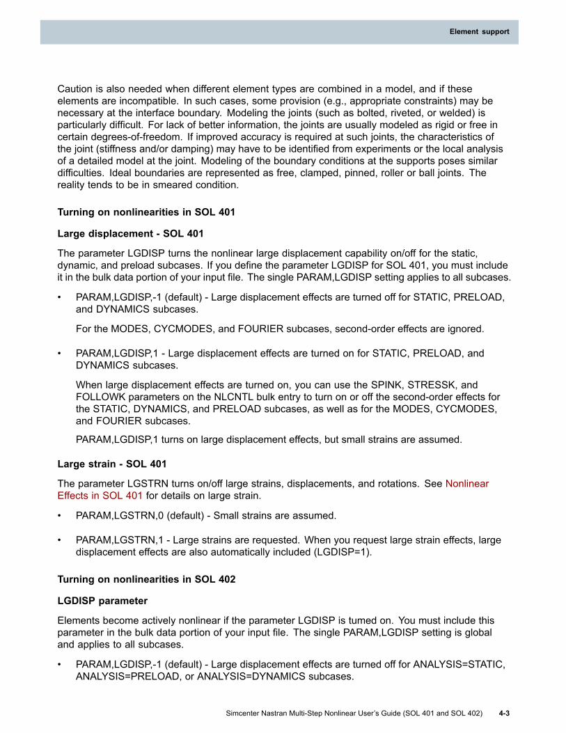
Element support
Caution is also needed when different element types are combined in a model, and if theseelements are incompatible. In such cases, some provision (e.g., appropriate constraints) may benecessary at the interface boundary. Modeling the joints (such as bolted, riveted, or welded) isparticularly difficult. For lack of better information, the joints are usually modeled as rigid or free incertain degrees-of-freedom. If improved accuracy is required at such joints, the characteristics ofthe joint (stiffness and/or damping) may have to be identified from experiments or the local analysisof a detailed model at the joint. Modeling of the boundary conditions at the supports poses similardifficulties. Ideal boundaries are represented as free, clamped, pinned, roller or ball joints. Thereality tends to be in smeared condition.
Turning on nonlinearities in SOL 401
Large displacement - SOL 401
The parameter LGDISP turns the nonlinear large displacement capability on/off for the static,dynamic, and preload subcases. If you define the parameter LGDISP for SOL 401, you must includeit in the bulk data portion of your input file. The single PARAM,LGDISP setting applies to all subcases.
• PARAM,LGDISP,-1 (default) - Large displacement effects are turned off for STATIC, PRELOAD,and DYNAMICS subcases.
For the MODES, CYCMODES, and FOURIER subcases, second-order effects are ignored.
• PARAM,LGDISP,1 - Large displacement effects are turned on for STATIC, PRELOAD, andDYNAMICS subcases.
When large displacement effects are turned on, you can use the SPINK, STRESSK, andFOLLOWK parameters on the NLCNTL bulk entry to turn on or off the second-order effects forthe STATIC, DYNAMICS, and PRELOAD subcases, as well as for the MODES, CYCMODES,and FOURIER subcases.
PARAM,LGDISP,1 turns on large displacement effects, but small strains are assumed.
Large strain - SOL 401
The parameter LGSTRN turns on/off large strains, displacements, and rotations. See NonlinearEffects in SOL 401 for details on large strain.
• PARAM,LGSTRN,0 (default) - Small strains are assumed.
• PARAM,LGSTRN,1 - Large strains are requested. When you request large strain effects, largedisplacement effects are also automatically included (LGDISP=1).
Turning on nonlinearities in SOL 402
LGDISP parameter
Elements become actively nonlinear if the parameter LGDISP is tumed on. You must include thisparameter in the bulk data portion of your input file. The single PARAM,LGDISP setting is globaland applies to all subcases.
• PARAM,LGDISP,-1 (default) - Large displacement effects are turned off for ANALYSIS=STATIC,ANALYSIS=PRELOAD, or ANALYSIS=DYNAMICS subcases.
Simcenter Nastran Multi-Step Nonlinear User’s Guide (SOL 401 and SOL 402) 4-3
Element support
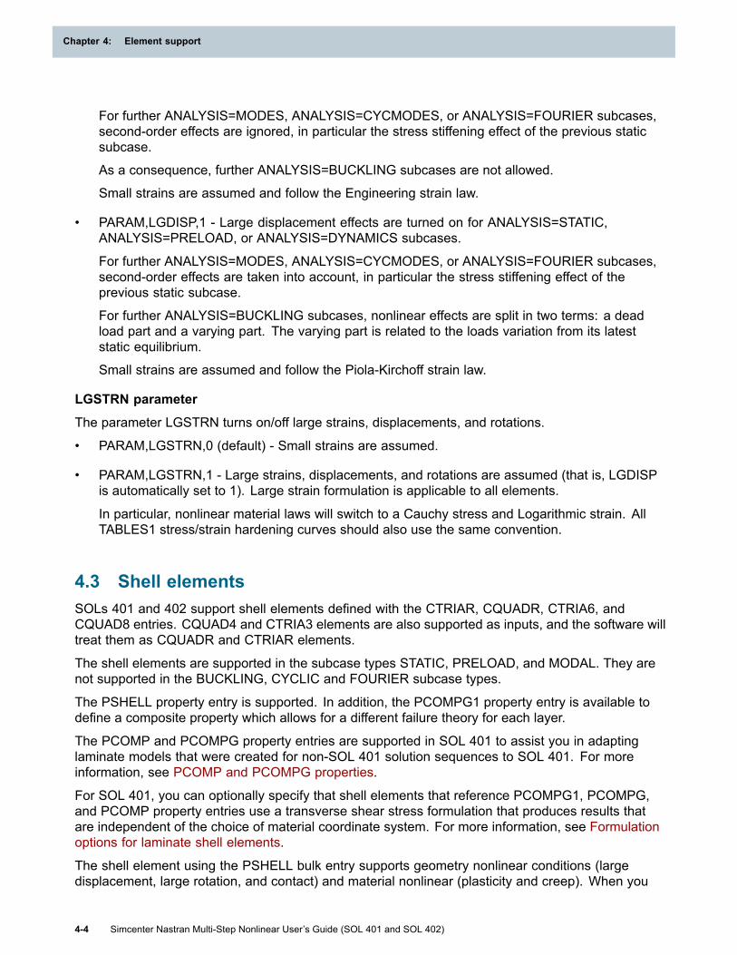
Chapter 4: Element support
For further ANALYSIS=MODES, ANALYSIS=CYCMODES, or ANALYSIS=FOURIER subcases,second-order effects are ignored, in particular the stress stiffening effect of the previous staticsubcase.
As a consequence, further ANALYSIS=BUCKLING subcases are not allowed.
Small strains are assumed and follow the Engineering strain law.
• PARAM,LGDISP,1 - Large displacement effects are turned on for ANALYSIS=STATIC,ANALYSIS=PRELOAD, or ANALYSIS=DYNAMICS subcases.
For further ANALYSIS=MODES, ANALYSIS=CYCMODES, or ANALYSIS=FOURIER subcases,second-order effects are taken into account, in particular the stress stiffening effect of theprevious static subcase.
For further ANALYSIS=BUCKLING subcases, nonlinear effects are split in two terms: a deadload part and a varying part. The varying part is related to the loads variation from its lateststatic equilibrium.
Small strains are assumed and follow the Piola-Kirchoff strain law.
LGSTRN parameter
The parameter LGSTRN turns on/off large strains, displacements, and rotations.
• PARAM,LGSTRN,0 (default) - Small strains are assumed.
• PARAM,LGSTRN,1 - Large strains, displacements, and rotations are assumed (that is, LGDISPis automatically set to 1). Large strain formulation is applicable to all elements.
In particular, nonlinear material laws will switch to a Cauchy stress and Logarithmic strain. AllTABLES1 stress/strain hardening curves should also use the same convention.
4.3 Shell elementsSOLs 401 and 402 support shell elements defined with the CTRIAR, CQUADR, CTRIA6, andCQUAD8 entries. CQUAD4 and CTRIA3 elements are also supported as inputs, and the software willtreat them as CQUADR and CTRIAR elements.
The shell elements are supported in the subcase types STATIC, PRELOAD, and MODAL. They arenot supported in the BUCKLING, CYCLIC and FOURIER subcase types.
The PSHELL property entry is supported. In addition, the PCOMPG1 property entry is available todefine a composite property which allows for a different failure theory for each layer.
The PCOMP and PCOMPG property entries are supported in SOL 401 to assist you in adaptinglaminate models that were created for non-SOL 401 solution sequences to SOL 401. For moreinformation, see PCOMP and PCOMPG properties.
For SOL 401, you can optionally specify that shell elements that reference PCOMPG1, PCOMPG,and PCOMP property entries use a transverse shear stress formulation that produces results thatare independent of the choice of material coordinate system. For more information, see Formulationoptions for laminate shell elements.
The shell element using the PSHELL bulk entry supports geometry nonlinear conditions (largedisplacement, large rotation, and contact) and material nonlinear (plasticity and creep). When you
4-4 Simcenter Nastran Multi-Step Nonlinear User’s Guide (SOL 401 and SOL 402)
Chapter 4: Element support

Element support
use a nonlinear plastic or creep material, the NLAYERS parameter is supported to define the numberof integration points through the thickness. The NLAYERS parameter supports 3, 5, 7, and 9 pointsthrough the thickness.
A composite shell element using the PCOMPG1 property bulk entry supports the geometry nonlinearconditions, but does not support material nonlinear.
The ZOFF field on the element entry is supported to offset the element reference plane.
CQUAD8 and CTRIA6 elements
• The CQUAD8 and CTRIA6 element formulations that the software uses for SOL 401 and 402,are different from the CQUAD8 and CTRIA6 element formulations that the software uses in theother solution sequences. You can use the SOL 401 and 402 formulations to model the followingmono-layer and laminate plane stress behaviors:
o Membrane stiffness (SOL 402 only)
o Membrane and bending stiffness (SOL 401 only)
o Membrane, bending, and transverse shear stiffness
o Membrane, bending, transverse shear, and coupled membrane-bending stiffness
The SOL 401 and 402 formulations do not support the following behaviors which are supported inother solution sequences:
o Plane strain.
o Bending stiffness only.
o Bending and transverse shear stiffness only.
The SOL 401 and 402 formulations have several advantages over the formulations used in theother solution sequences.
o They allow for higher aspect ratio of length to thickness before shear locking occurs.
o The CQUAD8 formulation is a heterosis formulation.
o The formulations use the K6ROT parameter to suppress grid point singularities by addingstiffness to the out-of-plane rotational DOF.
o When viewed normal to the reference plane of the element, the X- and Y-axes of the materialcoordinate system are consistent across the element. In the element formulations that areused in other solution sequences, the X- and Y-axes of the material coordinate systemvary across the element.
• The CQUAD8 heterosis formulation uses eight-noded serendipity shape functions for thetranslational DOF, and nine-noded Lagrange shape functions for the rotational DOF. The enrichedshape functions lead to better results although at some computational cost.
Because a ninth grid point is required for Lagrange shape functions and only eight actual gridpoints exist, the software creates internal DOF at the centroid of the element. The internal DOF
Simcenter Nastran Multi-Step Nonlinear User’s Guide (SOL 401 and SOL 402) 4-5
Element support

Chapter 4: Element support
functions as the ninth grid point for the element. After calculating the element matrices, thesoftware condenses the internal DOF prior to assembly into the global matrices.
By default, four Gauss points (2 x 2 integration) are used to integrate the membrane andtransverse shear stiffness, and nine Gauss points (3 x 3 integration) are used to integrate thebending and coupled membrane-bending stiffness.
• The CTRIA6 formulation uses six-noded serendipity shape functions for the translational androtational DOF.
By default, three Gauss points are used to integrate the membrane, bending, transverse shear,and coupled membrane-bending stiffness.
• When the software computes the element stiffness matrix for SOL 401 and 402 formulations, itadds rotational stiffness directly into the element stiffness matrix for the out-of-plane rotationalDOF. The rotational stiffness that the software adds is given by the following equation:
where K6ROT is the value of the K6ROT parameter, and D44 and D55 are entries in theconstitutive relation of the shell element. For example, the constitutive relation for a shell elementwhose geometry and material properties are symmetric about its midplane has the following form:
where:
Nx, Ny, Nxy In-plane forces
Mx, My, Mxy In-plane moments
εxo, εyo, γxyo Midplane strains
κx, κy, κxy Midplane curvatures
PSHELL property
• The MID1, MID2, and MID3 are all required. MID1 and MID2 must be explicitly defined, and theMID3 field defaults to the MID2 value.
• MID4 is optional. If MID4 is defined, MID1 and MID2 must be defined. MID4 is applied withrespect to the element plane regardless if ZOFF is defined or not. A ZOFF definition on theelement entry produces a coupling independent of the MID4. As a result, defining both MID4 andZOFF together will create two independent sources of coupling. If you define both MID4 andZOFF, the MID4 should represent an additional coupling which is unique to the ZOFF coupling.
4-6 Simcenter Nastran Multi-Step Nonlinear User’s Guide (SOL 401 and SOL 402)
Chapter 4: Element support

Element support
• When plastic or creep nonlinear materials are defined, the MID1, MID2, and MID3 must allbe the same, and MID4 must be undefined.
• 12I/T**3 and TS/T are only taken into account for elastic materials.
PCOMPG1 property
• The PCOMPG1 property entry is available to define a composite property which allows for adifferent failure theory for each layer.
• The MATFT defines the failure theory allowables for both shell and solid composites. MATFT isrequired to define allowables with the MAT9 and MAT11 material entries. If you are using theMAT1 material entry, you can optionally define the allowables with the MATFT, or you can specifythem on the MAT1 entry directly. For shell composites, only FT = HILL/HOFF/TSAI/STRN aresupported (NO FT = STRS/TS), and the transverse material properties are ignored for shells:
FT = HILL/HOFF: Zt, Zc, S13, S23 are ignored.
FT = TSAI: Zt, Zc, S13, S23, F13, F23 are ignored.
FT = STRN: Zet, Zec, Se13, Se23 are ignored.
• When a composite property is used, the software does not create a smeared, homogeneous shellrepresentation using classical lamination theory. Instead, an integration scheme similar to what isused for solid composites is used.
• Failure index and strength ratio output are supported for all failure indices.
• In SOL 402, Z0 is added to the offset introduced on the element bulk entry (ZOFFS). If elementforces are required, bending moments are given with respect to the updated neutral plane.
PCOMP and PCOMPG properties
• PCOMP and PCOMPG property entries are supported in SOL 401 to assist you in adaptinglaminate models that were created for non-SOL 401 solution sequences to SOL 401.
During the SOL 401 solve, when the software encounters a PCOMP or PCOMPG bulk entryin the input file, it internally converts it into a PCOMPG1 bulk entry. Because the PCOMPG1bulk entry does not have a LAM field, the software ignores the LAM field specification on thePCOMP or PCOMPG bulk entry when it performs the conversion. This can result in a loss oflaminate definition if the LAM field on the PCOMP or PCOMPG bulk entry that the softwareis converting is not blank.
Formulation options for laminate shell elements
• In SOL 401, you can optionally use laminate shell elements whose transverse shear stressformulation produces results that are independent of the choice of material coordinate system.The optional formulation is independent of the material coordinate system because it accounts forall three moments, Mx, My, and Mxy in Figure 1, whereas the default formulation ignores Mxy.Thus, depending on the stress state and the choice of material coordinate system, the defaultformulation may lead to less accurate results.
To use the formulation that accounts for all three moments, specify SYSTEM(715) = 1.
Simcenter Nastran Multi-Step Nonlinear User’s Guide (SOL 401 and SOL 402) 4-7
Element support

Chapter 4: Element support
Figure 4-1. Moments acting on a laminate shell element that lies in the XY-plane
Material support
• The MAT1 and MATT1 bulk entries define isotropic materials for any shell and composite property.
• The MAT2 and MATT2 bulk entries define anisotropic materials for any shell and compositeproperty.
• The MAT8 and MATT8 bulk entries define orthotropic materials for any shell and compositeproperty.
• The MAT9 and MATT9 bulk entries define anisotropic materials for any shell and compositeproperty.
• The MAT11 and MATT11 bulk entries define orthotropic materials for any shell and compositeproperty.
• The nonlinear plastic and creep material are only supported for the PSHELL.
• User defined materials defined with the UMAT external program are only supported for thePSHELL property.
• The TABLEM5 bulk entry defines tabular functions for progressive ply failure with the UD damagemodel.
• SOL 402 adds support for MATSR strain rate dependence.
Material coordinate system
4-8 Simcenter Nastran Multi-Step Nonlinear User’s Guide (SOL 401 and SOL 402)
Chapter 4: Element support

Element support
The material coordinate system is used to define the orientation of material properties whenorthotropic or anisotropic materials are selected. In addition, stress and strain results are alwaysoutput in the material coordinate system. The material coordinates are updated when large rotationoccurs.
The X-axis of the material coordinate system for the shell element is determined as follows:
• Option 1: If a material coordinate system is not explicitly selected on the element entry, the X-axisof the material coordinate system is, by default, aligned with the element edge defined by gridpoints G1 and G2. The X-axis can optionally be rotated by defining THETA on the element entry.
• Option 2: A material coordinate system can be selected with the MCID field on the element entry.The X-axis of the selected material coordinate system is projected onto the plane of the shellto define the shell material X-axis.
In addition, if a composite property is used for the element with the PCOMPG1 entry, a uniqueTHETA value can be defined for each ply. The THETA on the ply rotates the material x-axis for eachply relative to the element material x-axis as described above.
The material Z-axis is the positive out-of-plane shell normal defined by the right-hand-rule and thegrid point connection order. The material Y-axis is determined by the cross product of the materialX-axis and Z-axis.
Supported Loads
• Pressure loads are supported with the PLOAD, PLOAD2, or PLOAD4 bulk entries.
• General loads are supported with the FORCE, FORCE1, FORCE2, MOMENT, MOMENT1,MOMENT2, DAREA, and SLOAD.
• Body loads are supported with the GRAV, RFORCE, and RFORCE1. The RFORCE2 is notsupported.
In SOL 401, body loads are also supported with the ACCELi.
• Temperature loads with variation through the element thickness are not supported using theTEMPP1 bulk entry.
Shell element output summary
• Engineering stress and strain are always output.
• Stress and strain results are always output in the material coordinate system. The materialcoordinates are updated when large rotation occurs and large displacements effects arerequested with PARAM,LGDISP,1.
• Shell elements using a PSHELL support stress/strain results at grid or Gauss points. Stress andstrain is computed at the top and bottom of the element. The STRCUR describer, which requestsoutput at the middle plane, is not supported.
• Composite shell elements using the PCOMPG1 entry only supports stress/strain results at gridpoints.
• The CENTER, CUBIC, or SGAGE options on the STRESS and STRAIN case control commandsare not supported.
Simcenter Nastran Multi-Step Nonlinear User’s Guide (SOL 401 and SOL 402) 4-9
Element support

Chapter 4: Element support
• The OMID parameter which is used in other solutions to output stress and strain in the elementcoordinate system is not supported.
• The Z1 and Z2 fields on the PSHELL bulk entry, which define fiber distances for stresscalculations for other solution types, are not supported by SOLs 401 and 402.
• For composite shell elements, FI and SR is supported for all failure indices.
• The FORCE case control command can be used to request shell element resultants in materialcoordinates.
• Grid point forces are supported.
• Shell elements support surface-to-surface contact and surface-to-surface glue. Edge-to-edgeand surface-to-edge glue is not supported for shells in SOL 401. Both glue and contact resultsare support for the shell elements.
Additional information
• The SNORM parameter and bulk entry are only supported by the CTRIAR and CQUADRelements.
• The K6ROT parameter and bulk entry are only supported by the CTRIA6 and CQUAD8 elements.
4.4 Bar and beam elementsSOL 401 and SOL 402 supports bar and beam elements defined with the CBAR and CBEAM entries.The bar and beam elements support large displacements and rotations when large displacements arerequested with PARAM,LGDISP,1.
In SOL 402, CBAR defines the same element as CBEAM.
Physical properties
• The PBAR and PBARL entries define the physical properties for the BAR element.
• The PBEAM and PBEAML entries define the physical properties for the BEAM element.
• The intermediate stations defined with the X/XB field are permitted on the PBEAM and PBEAMLentries if, for example, the beam cross section properties change in the middle. Although, outputrequests are only supported at the ends A and B. The software ignores output requests at theintermediate locations (0 < X/XB < 1.0).
PBEAML section properties for SOL 402
• SOL 402 only supports different cross sections at ends A and B without any intermediatesections. A linear variation is assumed between the two ends.
• Beam sections of the following types are not supported: T1, T2, CHAN2, CROSS, H, BOX1,HEXA, HAT, and HAT1. In that case, the software will automatically create the equivalent PBEAMbulk entry and stress-recovery will not be performed. For beam sections of the following types:T1, T2, CHAN2, and H, equivalent profiles exist in other axes (T, CHAN, CHAN1, I or I1).
4-10 Simcenter Nastran Multi-Step Nonlinear User’s Guide (SOL 401 and SOL 402)
Chapter 4: Element support

Element support
• For beam sections of the following types: I, I1, CHAN, CHAN1, L, Z, T, BOX, and TUBE, the stressrecovery locations are located at the mid-thickness instead of the outer skin. Therefore, smalldeviations can be observed compared to other Simcenter Nastran solutions, such as SOL 401.
Materials
• MAT1 and MATT1 are supported.
• In SOL 401, MAT1 and MATS1 are supported to define a plastic material. For the nonlinearmaterial behavior to be included in the solution, you must reference the nonlinear materials fromthe PBARL and PBEAML property entries that define one of the following cross section types:TUBE, L (PBEAML only), I, CHAN, T, BOX, BAR, I1, CHAN1, Z, and ROD.
SOL 401 supports the cross section types on the PBARL and PBEAML that are not listed aboveand the PBAR and PBEAM entries if you reference a linear material entry. If you reference anonlinear material for these properties or cross section types, the solution ends with a fatal error.
You can optionally define a different cross section at ends A and B, and the software will computea linear variation. Cross section definitions at intermediate stations are ignored when a nonlinearmaterial is applied.
The CBAR and CBEAM elements in SOL 401 do not use a plastic hinge approach, which is usedby the CBEAM elements in SOL106. As a result, they are not limited to elastic-perfectly plasticmaterials (H=0.0) defined with the MATS1 bulk entry. For the CBAR and CBEAM elements inSOL 401, you can use the same plastic materials on the MATS1 entry which are supported forsolid and shell elements, such as H≠0.0 or stress-strain data.
• In SOL 401, MAT1 and MATCRP are supported to define a creep material. For the nonlinearmaterial behavior to be included in the solution, you must reference the nonlinear materials fromthe PBARL and PBEAML property entries that define one of the following cross section types:TUBE, L (PBEAML only), I, CHAN, T, BOX, BAR, I1, CHAN1, Z, and ROD.
The cross section types on the PBARL and PBEAML that are not listed above and the PBARand PBEAM entries are supported by SOL 401 if you reference a linear material entry. If youreference a nonlinear material for these properties or cross section types, the solution will endwith a fatal error.
You can optionally define a different cross section at ends A and B, and the software will computea linear variation. Cross section definitions at intermediate stations are ignored when a nonlinearmaterial is applied.
• In SOL 402, for nonlinear material, MATS1 can be used in PBARL and PBEAML propertyentities with profiles BAR, BOX, CHAN, CHAN1, I, I1, L, T, TUBE, and Z. If a plastic material isused (MATS1 bulk entry with TYPE=PLASTIC), the behavior is not limited to elastic-perfectlyplastic. The material behavior is calculated by numerical integration in the central section of theelement. It is constant for the whole element. To have a behavior close to a plastic hinge, youhave to use a finer mesh.
Supported loads
• The PLOAD1 bulk entry is supported to apply distributed loads.
Simcenter Nastran Multi-Step Nonlinear User’s Guide (SOL 401 and SOL 402) 4-11
Element support

Chapter 4: Element support
• Bar and beam elements also support the general loads that SOLs 401 and 402 support. Forexample the elements support forces using the FORCE, FORCE1, and body loads definedwith the GRAV and RFORCEi bulk entries.
SOL 401 also supports DAREA bulk entries and ACCELi body loads bulk entries.
Bar and beam element output summary
• Element results include stress, element force, total strain, elastic strain, and thermal strain.
• Stress and force output requests are only supported at the ends A and B. The software ignoresoutput requests at the intermediate locations (0 < X/XB < 1.0).
• Stress, strain, and force results are always output in the element coordinate system.
• The stress and strain output is similar to the existing format for other solutions, except that SOL401 and 402 do not compute the minimum and maximum values (S-MIN and S-MAX) and themargin of safety values (M.S. -T, and M.S. -C).
• The reported stresses SXC, SXD, SXE, and SXF are a combination of the normal and bendingstress reported in the element axial direction at the cross section locations C, D, E, and F.
• The element force output includes the bending moment and shear force in planes 1 and 2,axial force, total torque, and warping torque.
4.5 Spring and damper elements
Spring elements
You can use the CELAS1, CELAS2, CBUSH1D, and CBUSH elements in SOL 401 and SOL 402 todefine spring stiffness.
CELAS1- Scalar Spring Connection
• A single CELAS1 element connects two degrees-of-freedom at two different grid points. Itbehaves as a simple extension/compression or rotational spring, carrying either force or momentloads.
• If you define the CELAS1 element between non-coincident grid points, the CELAS1 element doesnot account for the distance between the connecting grid points when transferring loads. This isimportant when you expect your spring stiffness to carry transverse loads. The CELAS1 elementis safe to use when connecting coincident grid points. The CBUSH element is recommendwhen connecting non-coincident grid points.
• With the CELAS1 element, you can define either a constant or a nonlinear stiffness.
o You define the constant stiffness in the Ki field on the PELAS entry. The constant springstiffness definition is independent of the displacement.
o You define the nonlinear spring when the CELAS1 references both the PELAS and PELASTbulk entries. The TKNID field on the PELAST entry selects a TABLEDi entry, which definesthe force versus displacement data.
4-12 Simcenter Nastran Multi-Step Nonlinear User’s Guide (SOL 401 and SOL 402)
Chapter 4: Element support

Element support
• In SOL 401, the CELAS1 element does not support large displacement effects whenPARAM,LGDISP,1 is defined. You can include the CELAS1 element in a solution withPARAM,LGDISP,1 defined, but it should not be located in a region of the model where largerotations occur. If you define the CELAS1 as a nonlinear spring, the software uses the nonlinearspring definition whether large displacements are turned on or off.
SOL 402 does not have this limitation.
• You can request force and stress output for the CELAS1 element.
• In SOL 402, G1 and G2 must be grid points, not scalar points.
CELAS2- Scalar Spring Connection
• A single CELAS2 element connects two degrees-of-freedom at two different grid points. Itbehaves as a simple extension/compression or rotational springs, carrying either force ormoment loads.
• If you define the CELAS2 element between non-coincident grid points, the CELAS2 element doesnot account for the distance between the connecting grid points when transferring loads. This isimportant when you expect your spring stiffness to carry transverse loads. The CELAS2 elementis safe to use when connecting coincident grid points. The CBUSH element is recommendwhen connecting non-coincident grid points.
• The CELAS2 element only supports a constant spring stiffness which is independent of thedisplacement. This stiffness is defined in the Ki field on the CELAS2 entry. No property entryis used with the CELAS2 element.
• In SOL 401, the CELAS2 element does not support large displacement effects whenPARAM,LGDISP,1 is defined. You can include the CELAS2 element in a solution withPARAM,LGDISP,1 defined, but it should not be located in a region of the model where largerotations occur.
SOL 402 does not have this limitation.
• You can request force and stress output for the CELAS2 element.
• In SOL 402, G1 and G2 must be grid points, not scalar points.
CBUSH1D- Rod Type Spring Connection
• The CBUSH1D element is a one dimensional axial spring.
• The CBUSH1D element stiffness and forces are only axial. It can be used to define an axialspring between coincident or non-coincident grid points. When the grid points are coincident,the x-axis of the coordinate system selected with the CID field on the CBUSH1D entry becomesthe axial direction. When the grid points are non-coincident, the line from grid point A to gridpoint B is the element axis.
• In SOL 401, the CBUSH1D element connecting non-coincident grid points is the only spring thatsupports large displacement effects when PARAM,LGDISP,1 is defined.
SOL 402 does not have this limitation because in SOL 402 all springs non-coincident grid pointssupport large displacement effects.
Simcenter Nastran Multi-Step Nonlinear User’s Guide (SOL 401 and SOL 402) 4-13
Element support
Chapter 4: Element support
• A CBUSH1D element connecting coincident grid points does not support large displacementeffects when PARAM,LGDISP,1 is defined. In this case, the CBUSH1D element axis remainsfixed.
• The CBUSH1D element supports either a constant or a nonlinear stiffness option.
The constant spring stiffness definition is independent of the displacement and is defined with theK field on the on the PBUSH1D entry.
The nonlinear spring definition is a force versus displacement table. The nonlinear spring data isused when large displacements are turned on or off with the parameter LGDISP.
The nonlinear spring is defined by the following fields in the continuation row on the PBUSH1Dentry:
o “SPRING” should be defined in the field 2 of the continuation row.
o "TABLE" should be defined in field 3 of the continuation row.
o The ID of a TABLEDi entry should be defined in field 4 of the continuation row.
o The TABLEDi entry defines the force versus displacement relationship.
• You can request force and stress output for the CBUSH1D element.
CBUSH- Defines a generalized spring.• A unique feature of the CBUSH element relative to the other spring elements is that it accounts
for the distance between the connecting grid points when transferring loads. As a result, it is asafe choice for connecting either coincident or non-coincident grid points.
• The CBUSH entry supports either a constant, or a nonlinear stiffness option:
o The constant spring stiffness definition is independent of the displacement. This stiffness isdefined in a “K” row on the PBUSH entry, following by a stiffness value for each of the sixdegree-of-freedom.
o The nonlinear spring definition is a force versus displacement table. The nonlinear spring isdefined when the CBUSH entry references both the PBUSH and PBUSHT bulk entries. TheTKNIDi fields on the PBUSHT select the force versus displacement tables. The softwareuses the nonlinear spring when large displacements are turned on or off with the parameterLGDISP.
• In SOL 401, the CBUSH element does not support large displacement effects whenPARAM,LGDISP,1 is defined. You can include the CBUSH element in a solution withPARAM,LGDISP,1 defined, but it should not be located in a region of the model where largerotations occur.
SOL 402 does not have this limitation.
• You can request force, stress, and strain output for the CBUSH element.
• The system cell 665 is available to globally turn off the computation of the CBUSH couplingmoments when the connecting grid points are not coincident. The system cell applies to allsolutions except for SOLs 402, 601, and 701.
4-14 Simcenter Nastran Multi-Step Nonlinear User’s Guide (SOL 401 and SOL 402)
Chapter 4: Element support

Element support
SYSTEM(665) = 0 (default) The coupling moments are computed.
SYSTEM(665) = 1 The coupling moments are not computed.
Damper elements
CDAMP1 and CDAMP2- Scalar Damper Connections
• A single CDAMP1/CDAMP2 element connects two different degrees-of-freedom at two differentgrid points. It behaves as a simple extension/compression or rotational damper, carrying eitherforce or moment loads in function of the relative speed between the two degrees-o- freedom.
• Both CDAMP1 and CDAMP2 elements must be defined between non-coincident grid points andthe initial position has no consequence on the damping force.
• With the CDAMP1 element, you can define a constant value of viscous damping using thePDAMP bulk entry.
With the CDAMP2 element, you can define a constant value of viscous damping directly in theCDAMP2 bulk entry. You do not need a reference to a material or property entry.
• In SOL 402, the G1 and G2 grid points must be grid points not scalar points.
You can request force and stress output for the CDAMP1 or CDAMP2 element. The value of thegeneralized force is defined by the equation:
where:
• C is the viscous damping defined in the PDAMP bulk entry for the CDAMP1 element, or directlydefined in the CDAMP2 bulk entry for the CDAMP2 element
• are the speeds of the DOF G1 and G2 in component C1 and C2
4.6 Rigid elementsSOLs 401 and 402 support the RBE2, RBAR, and RBE3 elements. In the modal subcases in whichANALYSIS=MODAL, CYCMODES, or FOURIER, the software represents the rigid elements with MPCequations. In the static, transient dynamics, and preload subcases in which ANALYSIS=STATICS,DYNAMICS, or PRELOAD, the software always represents RBE3 elements with MPC equations.
SOL 401 - RBE2 and RBAR in static, dynamics, and preload subcases
In SOL 401 subcases where ANALYSIS=STATICS, DYNAMICS, or PRELOAD, the RIGID casecontrol command controls whether the RBE2 and RBAR elements include large displacement effectsand thermal expansion.
When RIGID=STIFF or RIGID=AUTO (default) and large displacements are requested withPARAM,LGDISP,1, the RBE2 and RBAR elements use a stiff element method to compute the largedisplacement effects. With the stiff element method, the software internally replaces the RBE2 andRBAR elements with either a stiff beam element or a stiff spring element. The stiff element thenaccounts for large displacements and rotations, including thermal expansion.
Simcenter Nastran Multi-Step Nonlinear User’s Guide (SOL 401 and SOL 402) 4-15
Element support

Chapter 4: Element support
An alternate nonlinear multipoint constraint (MPC) method is available. When you include theRIGID=NONLIN option and large displacements are requested with PARAM,LGDISP,1, the RBE2and RBAR elements will use a nonlinear MPC method to compute the large displacement effects.The software recomputes the MPC relationships when the rigid elements rotate. The RIGID=NONLINoption couples all six DOF.
With the nonlinear MPC method, the software adds the dependent DOF to the multipoint constraintset (m-set), thus eliminating this DOF from the analysis set (a-set). As a result, if your modelincludes many RBE2 and RBAR elements, the nonlinear MPC method can be more efficient than thestiff element method.
The RIGID=NONLIN option does not support thermal expansion of the RBE2 and RBAR elements, soyou must use the stiff element method if thermal expansion is required. The stiff element methodis still used by default when large displacements are requested with PARAM,LGDISP,1. If you arerunning a small displacement analysis with PARAM,LGDISP,-1 (default), and you require thermalexpansion, you must explicitly define RIGID=STIFF.
When the RIGID=NONLIN option is selected, the coefficients for the constraint equation can vary ateach iteration based on the change in the rotations for the independent grid. As a result, the multipointconstraint equations and the multipoint constraint transformations are recomputed. For models whichinclude many nonlinear rigid elements with many iterations, this will increase the solution time.
See SOL 401 - Nonlinear MPC mathematical description below.
Input summary for SOL 401
• When RIGID=AUTO (default) and PARAM,LGDISP,-1 (default), the software automaticallyapplies the RIGID=LINEAR option. Specifically, the RBE2 and RBAR elements do not includelarge displacement effects or thermal expansion.
• When RIGID=AUTO (default) and PARAM,LGDISP,1, the software automatically applies thebehavior consistent with RIGID=STIFF and PARAM,LGDISP,1. Specifically, the RBE2 and RBARelements use a stiff element method to compute large displacement effects, and they includethermal expansion.
• When RIGID=STIFF and PARAM,LGDISP,-1 (default), the RBE2 and RBAR elements do notinclude large displacement effects, but they do include thermal expansion.
• When RIGID=STIFF and PARAM,LGDISP,1, the RBE2 and RBAR elements use a stiff elementmethod to compute large displacement effects, and they include thermal expansion.
• When RIGID=NONLIN and PARAM,LGDISP,-1 (default), the RBE2 and RBAR elements donot include large displacement effects or thermal expansion. The behavior is the same asRIGID=LINEAR.
• When RIGID=NONLIN and PARAM,LGDISP,1, the RBE2 and RBAR elements use a nonlinearMPC method to compute large displacement effects, but they do not include thermal expansion.
• When RIGID=LINEAR, the RBE2 and RBAR elements do not include large displacement effectsor thermal expansion. This behavior is independent of the PARAM,LGDISP setting.
• The following occurs when thermal expansion is requested with the RIGID=STIFF option.
4-16 Simcenter Nastran Multi-Step Nonlinear User’s Guide (SOL 401 and SOL 402)
Chapter 4: Element support

Element support
For the RBAR element, the software computes an average TEMP(LOAD) and TEMP(INIT) for theelement from the grid point values.
For the RBE2 element, the software computes an average TEMP(LOAD) and TEMP(INIT) foreach leg of the element using the values on the independent/dependent grid pairs such that eachleg can have a different thermal strain if the temperatures vary at the grids.
The rigid element thermal strains are calculated from
εthermal = α(AVGTEMP(LOAD) – AVGTEMP(INIT))
If TEMP(LOAD) or TEMP(INIT) are not defined, they are assumed to be zero.
• MPCFORCE and GPFORCE output are supported with all of the rigid elements. Since thesoftware internally replaces an RBAR or RBE2 with a stiff beam or spring element whenRIGID=STIFF, these elements are no longer represented as MPC equations. As a result,MPCFORCE output is not applicable to these elements. GPFORCE and FORCE output isapplicable.
• When RIGID=STIFF and you combine static, transient dynamics, and preload subcases in whichRBE2 and RBAR elements include large displacement effects and modal subcases in your inputfile, the RBE2 and RBAR elements are treated as stiff beams in a static, transient dynamics,and preload subcase, but are still treated as MPC equations in a modal subcase. If your rigidelements experience large rotations in a static, transient dynamics, and preload subcases,a sequentially dependant modal subcase will use the deformed state from the previous staticssubcase, but the MPC equations are still relative to the unchanging global coordinate system.
With the RIGID=STIFF option, to compute large displacement effects and thermal expansion, thesoftware internally replaces the RBE2 and RBAR elements with either a stiff beam element, ora stiff spring element. A coincident grid tolerance is used to determine if a beam or a spring isused. For the RBAR, if the distance between the connecting grids is less than the tolerance, the stiffspring formulation is used. For the RBE2, if the distance between the grid defined in the GN field onthe RBE2 entry, and any of the grids defined in the GM fields on the RBE2 entry, is less than thetolerance, the stiff spring formulation is used. You can optionally define the coincident grid toleranceexplicitly with the parameter RGLCRIT. By default, it is automatically computed by the software:
Coincident Grid Tolerance = 1E-6 * LMODEL (units=length)
where LMODEL is the largest dimension of the model determined by the software.
You can optionally define the beam stiffness and area explicitly using the parameters RGBEAME andRGBEAMA, respectively. By default, they are automatically computed by:
Beam Stiffness = 1e+2 * EMAX (units=force/length^2)
Beam Area = (LMODEL * 1e-2)^2 (units=length^2)
where EMAX is the largest Young’s modulus in the model. If no material is specified in the model,EMAX is set to 1.0E12.
You can optionally define the spring stiffness explicitly using the parameter RGSPRGK. By default, itis automatically computed by:
Spring Stiffness = EMAX * LMODEL (units = force/length)
See the RIGID case control command.
Simcenter Nastran Multi-Step Nonlinear User’s Guide (SOL 401 and SOL 402) 4-17
Element support

Chapter 4: Element support
SOL 401 - Nonlinear MPC mathematical description
Nonlinear MPCs are an alternate method of enforcing rigid constraints in a nonlinear analysis. Youcan request the nonlinear MPCs with RIGID=NONLIN or RIGID=AUTO for RBAR or RBE2 elements.The desired effect of this methodology is to ensure that the length of the segment connecting theindependent node to the dependent node remains constant.
Let and be the respective coordinates of the independent and dependent nodes inthe reference configuration.
and is the length of this vector.
After deformation , the new position of the independent node will be:
The rotations associated with the independent node can be represented by and the corresponding
rotation matrix by .
The current position of the independent node can then be obtained by:
In index notation, this can be written as:
To obtain :
The finite rotation vector associated with the independent node can be represented by:
Let represent the largest absolute component of the rotation vector, that is,
.
4-18 Simcenter Nastran Multi-Step Nonlinear User’s Guide (SOL 401 and SOL 402)
Chapter 4: Element support

Element support
The rotation magnitude can then be defined as:
And the rotation axis can be defined as:
The skew symmetric matrix associated with the rotation vector is then given by:
The rotation matrix is then the exponential of this skew symmetric matrix:
Constraints:
Restating the equation for translations of the dependent node in terms of translations and rotations ofthe independent node:
The coefficients for the translations of the independent grid in the constraint equation then are:
The result of this equation is an identity matrix as expected.
The coefficients for rotations of the independent node that affect the translations of the dependentnode are:
Simcenter Nastran Multi-Step Nonlinear User’s Guide (SOL 401 and SOL 402) 4-19
Element support

Chapter 4: Element support
Since, the constraint coefficients depend on the rotation matrix, they can potentially change in eachiteration. The enforcement of this constraint in each iteration by updating the constraint matrix is themain difference between RIGID=LINEAR and RIGID=NONLIN.
SOL 402 - RBE1, RBE2, and RBAR element options
• RBE2 and RBE3 elements support large displacements (PARAM,LGDISP,1) and large strains(PARAM,LGSTRN,1).
• The RIGID case control command is ignored and does not affect the behavior of the spring.
• The TEMP(LOAD) and TEMP(INIT) value used on RBAR elements is an average calculatedfrom the grid point values. On RBE2 elements, an average TEMP(LOAD) and TEMP(INIT) iscalculated for each leg of the element using the values on the independent/dependent grid pairssuch that each leg can have a different thermal strain if the temperatures vary at the grids.
The rigid element thermal strains are calculated from:
εthermal = α(AVGTEMP(LOAD) – AVGTEMP(INIT))
If TEMP(LOAD) or TEMP(INIT) are not defined, they are assumed to be zero.
• All rigid elements support MPCFORCE and GPFORCE output.
• GPFORCE output correctly accounts for large displacements.
4.7 Generalized plane strain (SOL 401)A special plane strain formulation called generalized plane strain is available as an optional extensionto the standard plane strain formulation. Both formulations use the CPLSTN3, CPLSTN4, CPLSTN6,and CPLSTN8 plane strain element types. To invoke the generalized plane strain option, theplane strain elements need to reference a PGPLSN property bulk entry. The generalized planestrain option is only supported in SOL 401, and is only applicable to small strain, small deflectionstructural analyses. These structural analyses include linear static, creep, and plasticity analyses,and combination creep and plasticity analysis.
Analysis with the generalized plane strain formulation is highly specialized and typically used toevaluate the behavior of gas turbine compressor and turbine blades. For such an analysis, you meshthe cross section of the blade with CPLSTN3, CPLSTN4, CPLSTN6, or CPLSTN8 elements. All ofthe elements in the mesh should reference a single PGPLSN property bulk entry.
With the PGPLSN bulk entry, you can specify the following data:
• The material bulk entry that is referenced by the PGPLSN bulk entry. MAT1 and MAT3 materialbulk entries can be referenced.
• The control grid point. The control grid point is the location where out-of-plane loads or enforceddisplacements are applied to the set of elements that reference the PGPLSN bulk entry.
4-20 Simcenter Nastran Multi-Step Nonlinear User’s Guide (SOL 401 and SOL 402)
Chapter 4: Element support

Element support
• The element thickness in the undeformed state.
• Optional user-defined additive normal stiffness and rotational stiffness values.
• You can specify time-varying added normal and rotational stiffness terms. To do so, in an addedstiffness field on the PGPLSN entry, enter the identification number of a TABLEDi bulk entry. Onthe TABLEDi entry,you will list tabular data to define how the added stiffness term varies with time.
For the generalized plane strain analysis, Simcenter Nastran calculates the standard in-plane planestrain stiffness, but also calculates three net out-of-plane stiffness values relative to the displacementcoordinate system of the control grid point. Consequently, how you specify the displacementcoordinate system for the control grid point is very important. You should specify the displacementcoordinate system of the control grid point such that one axis is normal to the cross section and theother two axes are parallel to the principal axes of the cross section. By so doing, the three netout-of-plane stiffness values that Simcenter Nastran calculates represent the normal stiffness of thecross section, and the two bending stiffness for symmetrical bending of the cross section.
Because the CPLSTN3, CPLSTN4, CPLSTN6, and CPLSTN8 plane strain elements can only bedefined in the XY- or XZ-planes of the basic coordinate system, the direction normal to the crosssection is always in the Z- or Y-direction, respectively of the basic coordinate system. SimcenterNastran checks that one of the axes of the displacement coordinate system of the control grid pointcoincides with the correct normal direction and issues an error if one does not.
Simcenter Nastran does not check the other two coordinate directions of the displacement coordinatesystem for the control grid point. It is your responsibility to assure that these directions are parallel tothe principal axes of the cross section.
If you specify additive stiffness, the normal stiffness is added to the normal stiffness that SimcenterNastran calculates for the cross section . The additive rotational stiffness values are added to thebending stiffness values as follows:
• If the model lies in the XY-plane of the basic coordinate system, the KR1 value on the PGPLSNbulk entry is added to the bending stiffness about the X-axis of the displacement coordinatesystem of the control grid point. the KR2 value on the PGPLSN bulk entry is added to the bendingstiffness about the Y-axis of the displacement coordinate system of the control grid point.
• If the model lies in the XZ-plane of the basic coordinate system, the KR1 value on the PGPLSNbulk entry is added to the bending stiffness about the X-axis of the displacement coordinatesystem of the control grid point. the KR2 value on the PGPLSN bulk entry is added to the bendingstiffness about the Z-axis of the displacement coordinate system of the control grid point.
You can apply loads to the control grid point and to the generalized plane strain element mesh. At thecontrol grid point, you can account for the centrifugal force that is attributable to the portion of theblade from the cross section you are modeling to the blade tip. To allow you to define a mechanicallyequivalent loading at the control grid point, you can specify not only a force that acts normal to thecross section, but also the bending moments that act on the cross section about axes parallel to theprincipal axes of the cross section.
To the generalized plane strain mesh, apply surface tractions, body forces, and in-plane enforceddisplacements that you want to include in the analysis. For example, you can apply aerodynamicforces to the grid points that lie on the periphery of the mesh.
Simcenter Nastran Multi-Step Nonlinear User’s Guide (SOL 401 and SOL 402) 4-21
Element support

Chapter 4: Element support
From the net out-of-plane stiffness values and the loads that are applied to the control grid point,Simcenter Nastran calculates the thickness change over the cross section. Similar to planesremaining plane in pure bending of beams, Simcenter Nastran enforces that the surface defined bythe thickness change is planar. From the thickness change over the cross section, Simcenter Nastrancalculates the out-of-plane strain of the elements at the grid locations. During the solution of the finiteelement model, Simcenter Nastran uses the out-of-plane strain and any surface tractions, bodyforces, and in-plane enforced displacements that you specified.
If an enforced displacement and enforced rotations are applied at the control grid point, the thicknesschange of the cross section is directly specified. From the thickness change, Simcenter Nastrancalculates the out-of-plane strain directly and the solution of the finite element model is as before.
Note the generalized plane strain element is not supported by glue or contact regions.
The following constitutive models are available with generalized plane strain elements:
• To model plasticity of an isotropic material, use the MAT1 and MATS1 bulk entries in combination.
• To model plasticity of an isotropic material with temperature-dependent properties, use somecombination of the MAT1, MATS1, MATT1, TABLEST, and TABLES1 bulk entries.
• To model plasticity of an orthotropic material, use the MAT3 and MATS1 bulk entries incombination. The elastic portion of the response is orthotropic, and the plastic portion of theresponse is isotropic.
• To model plasticity of an orthotropic material with temperature-dependent properties, use somecombination of the MAT3, MATS1, MATT3, TABLEST, and TABLES1 bulk entries. The elasticportion of the response is orthotropic, and the plastic portion of the response is isotropic.
• To model creep of an isotropic material, use the MAT1 and MATCRP bulk entries in combination.
• To model creep of an isotropic material with temperature-dependent properties, use the MAT1,MATT1, and MATCRP bulk entries in combination.
• To model creep of an orthotropic material, use the MAT3 and MATCRP bulk entries in combination.
• To model creep of an orthotropic material with temperature-dependent properties, use the MAT3,MATT3, MATCRP, and TABLEM1 bulk entries in combination. The elastic portion of the responseis orthotropic, and the creep portion of the response is isotropic.
For additional information, see the PGPLSN bulk entry in the Simcenter Nastran Quick ReferenceGuide.
4.8 Element addition and removalSOL 401 supports the capability to add or remove elements during a solution at pre-defined timepoints. For example, you can represent a material removal process while the model is in a loadedstate.
The software adds or removes the associated mass and stiffness from the solution. Damping isnot added or removed.
4-22 Simcenter Nastran Multi-Step Nonlinear User’s Guide (SOL 401 and SOL 402)
Chapter 4: Element support

Element support
In addition, SOL 401 also supports the capability to remove elements based on a state of strain atthe element integration points. This is useful to represent a rupture condition. You can define theremoval strain state using an inelastic strain (plasticity and creep), or using the total mechanical strain(elastic+inelastic mechanical strain).
The ELAR case control command is available to select the element add/removal set. The ELARcommand can be defined globally (above the subcases), or in a static or dynamic subcase. SeeSubcase rules.
You define the add and removal of elements with the ELAR and ELAR2 bulk entries. The ELAR entryselects the GRPID bulk entry which is useful when you have a large number of elements to add orremove. The ELAR2 entry lists elements directly for add or removal, so it is useful when you havefewer elements. The ELARADD bulk entry is also available to combine multiple ELAR and ELAR2bulk entries into a single add/removal set.
ELAR and ELAR2 bulk entry summary
• The TYPE field defines the addition/removal criteria type. See the ELAR and ELAR2 entriesfor the format of each type.
TYPE = TIME: Element Addition/Removal based on time.
TYPE = RINELE: Element removal (rupture) based on the effective inelastic strain.
TYPE = RMECHE: Element removal (rupture) based on the effective mechanical strain.
• For TYPE=TIME, AC and RC define the addition time and removal time, respectively.
If the time defined for AC or RC is in the time range for a subcase, but not precisely a solutiontime defined by the TSTEP1 bulk entry, a new solution time will be created for the elementaddition or removal. You can optionally request output for all time steps, including time stepscreated for the element addition or removal, by defining NOUT=ALL on the TSTEP1 bulk entry.
If you define the ELAR case control command above the subcase level (global definition), youmust define AC or RC in the time range of one of the subcases. Otherwise, the software willnot add or remove the associated elements.
If you define the ELAR case control command in a subcase, it is recommended that you defineAC or RC in the time range for the subcase. Although, if AC or RC fall outside the range ofthe subcase time, the additions and removal will occur at the end time for the subcase. Anexception is if both AC and RC are defined for the same element in the same subcase. In thiscase, the addition will occur at the end time for the subcase, the removal will be ignored, anda warning will occur.
• The addition delta time (AD field) and removal delta time (RD field) are time intervals used to addor remove the element mass and stiffness. The delta time options slow the transition of adding orremoving elements which helps to prevent convergence problems.
If the delta time is greater than the time remaining in the subcase, it will be adjusted to equalthe remaining time in the subcase.
If you define -1 in the AD or RD fields, the software will ramp the element addition or removalover the remaining subcase time.
When the AD and RD fields are undefined, an element addition or removal occurs instantly.
Simcenter Nastran Multi-Step Nonlinear User’s Guide (SOL 401 and SOL 402) 4-23
Element support

Chapter 4: Element support
• For TYPE = RINELE, you enter the effective inelastic strain in the RC field in which the elementwill be removed. The strain value you define includes strain contributions from both plasticityand creep materials if both are defined on an element. Plastic and creep strain output can berequested with the PLSTRN and CRSTRN case control commands, respectively.
• For TYPE = RMECHE, you enter the effective mechanical strain in the RC field in which theelement will be removed. The strain value you define includes the elastic and inelastic strains.Elastic strain output can be requested with the ELSTRN case control command. For example, ifan element has both plastic and creep strain, the effective mechanical strain would be the sum ofthe effective elastic, effective plastic, and effective creep strains. If the material is a user definedmaterial (UMAT), the effective mechanical strain is the equivalent mechanical strain computedfrom mechanical strain components.
Additional information
• For TYPE=TIME, the following elements are supported:
The 3D solids elements CTETRA, CHEXA, CPENTA, CPYRAM with properties defined with thePSOLID or PCOMPS entry.
The axisymmetric elements CQUADX4, CQUADX8, CTRAX3, CTRAX6.
The plane strain elements CPLSTN3, CPLSTN4, CPLSTN6, CPLSTN8 including when definedas a generalized plane strain element.
The plane stress elements CPLSTS3, CPLSTS4, CPLSTS6, CPLSTS8.
The chocking elements CCHOCK3, CCHOCK4, CCHOCK6, CCHOCK8.
The bar and beam elements CBAR, CBEAM.
The shell elements CTRIAR, CQUADR, CTRIA6, CQUAD8, CQUAD4, CTRIA3 with propertiesdefined with the PSHELL, PCOMP, or PCOMPG entries.
The spring elements CELAS1, CELAS2, CBUSH1D, CBUSH.
• For TYPE=RINELE, the following elements are supported:
The 3D solids elements CTETRA, CHEXA, CPENTA, CPYRAM defined with the PSOLID entry.
The axisymmetric elements CQUADX4, CQUADX8, CTRAX3, CTRAX6.
The plane strain elements CPLSTN3, CPLSTN4, CPLSTN6, CPLSTN8 including when definedas a generalized plane strain element.
The plane stress elements CPLSTS3, CPLSTS4, CPLSTS6, CPLSTS8.
The chocking elements CCHOCK3, CCHOCK4, CCHOCK6, CCHOCK8.
The shell elements CTRIAR, CQUADR, CTRIA6, CQUAD8, CQUAD4, CTRIA3 with propertiesdefined with the PSHELL entry.
• For TYPE=RMECHE, the following elements are supported:
The 3D solids elements CTETRA, CHEXA, CPENTA, CPYRAM defined with the PSOLID orPCOMPS entry.
The axisymmetric elements CQUADX4, CQUADX8, CTRAX3, CTRAX6.
4-24 Simcenter Nastran Multi-Step Nonlinear User’s Guide (SOL 401 and SOL 402)
Chapter 4: Element support

Element support
The plane strain elements CPLSTN3, CPLSTN4, CPLSTN6, CPLSTN8 including when definedas a generalized plane strain element.
The plane stress elements CPLSTS3, CPLSTS4, CPLSTS6, CPLSTS8.
The chocking elements CCHOCK3, CCHOCK4, CCHOCK6, CCHOCK8.
The shell elements CTRIAR, CQUADR, CTRIA6, CQUAD8, CQUAD4, CTRIA3 with propertiesdefined with the PSHELL, PCOMP, or PCOMPG entries.
• The elements CMASSi, CONMi, and cohesive elements are not supported for adding andremoving.
• The software automatically adds or removes from the solution any loads, boundary conditions, orunconnected grid points that are referenced by elements which are added or removed.
Exceptions:
- Contact and glue conditions are not supported on elements being added or removed.
- MPCs or rigid elements cannot be defined on the same grid points of elements being added orremoved.
- A distributed load defined with the FORCDST bulk entry is not supported with the elementaddition or removal.
• When you reference elements by an element addition/removal set to be added at a solution timepoint, the software considers those elements as inactive at the start of the solution. The softwareconsiders all other elements as active at the start of the solution.
Relative to a sequence of sequentially dependent (SD) subcases, elements can only be addedone time, and elements can only be removed one time. As a result, elements which are removedcannot be readded.
For example, you can remove an element which was active at the start of the solution, or you canremove an element which became active at a solution time point during the solution.
• You can only define one removal criteria for an element. For example, for the same element, youcannot define both a removal based on a strain state and a removal based on time.
• Subcase rules
o Element addition and removal can occur in a statics or dynamics subcase. The staticssubcase in which nonlinear buckling is requested with the NLARCL=ID case controlcommand is not supported.
Element addition and removal can not occur in a preload, modal, cyclic, or Fourier subcase.Although, the add/remove status is retained for these subcases if they are sequentiallydependent. For example, if an element is added in a static subcase and the next subcaseis a sequentially dependent modal subcase, the added element will be active in the modalsubcase.
o You can define a global definition of an element add/remove set by placing the ELAR casecontrol command above the subcase level. The global definition is the most flexible and leastrestrictive option. You can define element addition or removal for times, or for strain state,across all static and dynamic subcases with a global definition.
Simcenter Nastran Multi-Step Nonlinear User’s Guide (SOL 401 and SOL 402) 4-25
Element support

Chapter 4: Element support
o You can define a specific subcase definition of an element add/remove set by includingthe ELAR case control command in a static or dynamic subcase. For element addition,the specific subcase definition is restricted to only the first static or dynamic subcase in asequence of sequentially dependent subcases. For element removal, you can include theELAR case control command in any static or dynamic subcase.
o If you include a non-sequentially dependent (NSD) subcase, the state of the solution is resetback to the initial state, including the element add and remove status and the solution timewhich is reset back to 0.0. When you define an NSD subcase, you are restarting the solution.
4.9 Error estimator for mesh refinement (SOL 401)You can request stress norm, stress error norm, strain energy norm, and strain energy error normoutput when using SOL 401. The output is computed and stored on an individual element basis.Pre/Post uses the output for adaptive meshing.
The output is supported for the following element types:
Solid elements CHEXA, CPENTA, CPYRAM, CTETRA (excludes CHEXA and CPENTAelements referencing PCOMPS bulk entries)
Axisymmetric elements CQUADX4, CQUADX8, CTRAX3, CTRAX6
Plane strain elements CPLSTN3, CPLSTN4, CPLSTN6, CPLSTN8 (includes elementsreferencing PGPLSN bulk entries)
Plane stress elements CPLSTS3, CPLSTS4, CPLSTS6, CPLSTS8
• The stress norm is calculated from:
• The stress error norm is calculated from:
• The strain energy norm is calculated from:
• The strain energy error norm is calculated from:
where
Ω is the element volume,
4-26 Simcenter Nastran Multi-Step Nonlinear User’s Guide (SOL 401 and SOL 402)
Chapter 4: Element support

Element support
σunaveraged is the unaveraged stress vector,
σaveraged is an averaged stress vector computed at a grid point using the stress vectors from elementsconnected to the grid point,
D matrix is the constitutive relation.
When computing σaveraged, stress values are not averaged across different element families, materialproperties, material coordinate systems, orientation angles in 2D solid elements, and thicknesses inplane stress elements.
You use the STRESS, STNERGY and STEP describers on the ADAPTERR case control commandto request the output.
• The ADAPTERR case control command must be defined above the subcases (globally).
• The STRESS describer requests the stress norm and the stress error norm.
• The STNERGY describer requests the strain energy norm and strain energy error norm.
• You can specify both the STRESS and STNERGY describers to request stress norm, stress errornormal, strain energy norm and strain energy error norm output.
• The software always outputs the maximum value on each element, for each output typerequested, by comparing the values from all solution steps. In addition, if you specify the STEPdescriber, the software will output what you have requested at the output increment steps definedwith the TSTEP1 entries.
For additional information, see the ADAPTERR case control command.
4.10 Progressive failure analysis in solid compositesYou can model progressive ply failure in composite laminates that are meshed with composite solidelements. Simcenter Nastran supports a unidirectional fibre reinforced ply damage model (UD) andan enhanced unidirectional fibre reinforced ply damage model (EUD).
The UD model is based on a model developed by Ladeveze and Le Dantec (Damage modeling of theelementary ply for laminated composites, Composites Science and Technology 43, 1992) in whichdamage is linked to the transverse normal stress and in-plane shear stress.
The EUD model is obtained by further splitting damage variables in UD into two parts: diffusedamage related parts, and crack density dependent parts. The EUD model damage depends on thetransverse cracking of the ply.
Both of the models can account for:
• Damage in fibre direction 11, damage in shear direction 12, damage in transverse direction 22.
• Damage linked to the stresses in the out-of-plane direction.
• Damage mechanisms: fibre breaking, diffuse damage (fibre-matrix debonding), transversecracking in matrix.
• Damage linked to time delay effects.
Simcenter Nastran Multi-Step Nonlinear User’s Guide (SOL 401 and SOL 402) 4-27
Element support

Chapter 4: Element support
• Coupling with plasticity.
• Stress/strain-dependent elastic modulus.
The procedure for estimating ply damage is iterative. Using the material properties in the undamagedstate, Simcenter Nastran makes an initial calculation of the stress state. Simcenter Nastran uses thisstress state in the unidirectional ply model to calculate an initial estimate of ply damage. Based onthese damage values, Simcenter Nastran calculates the material properties in the damaged state.With these values for the material properties, Simcenter Nastran solves the model to obtain theupdated stress state. Simcenter Nastran uses the updated stress state in the ply model to calculate asecond estimate of the ply damage, and continues iterating until the ply damage values converge.
The converged damage values are termed the static damage. If you optionally include time delayeffects, the final damage values for the time step are the static damage values adjusted for thetime delay.
To use the progressive ply failure capability, model the laminate with CHEXA and CPENTA solidelements that reference PCOMPS bulk entries. In the MIDi fields of the PCOMPS bulk entries, enterthe MID of MAT11 bulk entries to define the linear elastic properties of the plies in the undamagedstate. To define the material properties and parameters that are related to progressive ply failuremodel, include MATDMG bulk entries that have the same MID as the MAT11 bulk entries. To obtainply failure results output, include a PFRESULTS case control command.
You can use the CHEXCZ and CPENTCZ cohesive elements to model the interface between thedifferent plies. In this case, you model the plies with composite solid elements with a cohesiveelement defined between the plies.
Additional details for the UD and EUD models:
• The UD and EUD models are both supported by composite solid elements.
• The UD and EUD models only support orthotropic materials. The material ID defined for acomposite ply on the PCOMPS entry references a MAT11 and a MATDMG. You enter PFA inthe FTi field on the PCOMPS entry.
• The UD and EUD models both require that you specify PARAM,MATNL,1 to activate the damageproperty. By default, PARAM,MATNL,-1, and PFA behavior is turned off.
• The UD and EUD models both support geometry nonlinear.
• You can include both the UD and EUD models on different plies on the same composite definedwith the PCOMPS entry.
• The PFRESULTS case control command includes the CRKDSTY describer to request the crackdensity output. The ODAMGPFR datablock stores the crack density output.
When you include the CRKDSTY describer on the PFRESULTS command, the EUD modeloutputs the transverse crack density output. It is a scalar value reported at the mid ply location foreach ply at the element corners. The crack density is dimensionless.
• Both the UD and EUD models allow you to include coupling with plasticity. If you have includedthe coupling with plasticity, you can define the PLSTRN case control command in a subcase to
4-28 Simcenter Nastran Multi-Step Nonlinear User’s Guide (SOL 401 and SOL 402)
Chapter 4: Element support
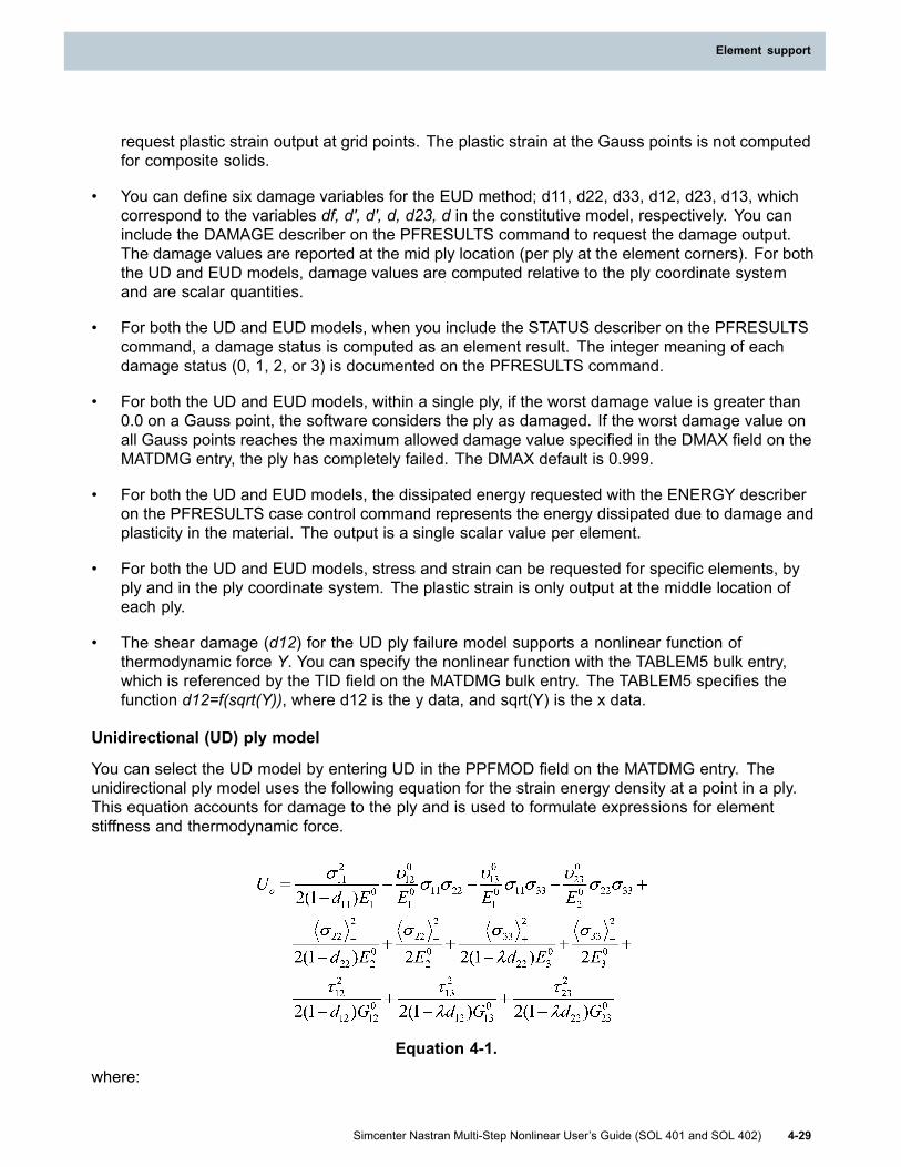
Element support
request plastic strain output at grid points. The plastic strain at the Gauss points is not computedfor composite solids.
• You can define six damage variables for the EUD method; d11, d22, d33, d12, d23, d13, whichcorrespond to the variables df, d', d', d, d23, d in the constitutive model, respectively. You caninclude the DAMAGE describer on the PFRESULTS command to request the damage output.The damage values are reported at the mid ply location (per ply at the element corners). For boththe UD and EUD models, damage values are computed relative to the ply coordinate systemand are scalar quantities.
• For both the UD and EUD models, when you include the STATUS describer on the PFRESULTScommand, a damage status is computed as an element result. The integer meaning of eachdamage status (0, 1, 2, or 3) is documented on the PFRESULTS command.
• For both the UD and EUD models, within a single ply, if the worst damage value is greater than0.0 on a Gauss point, the software considers the ply as damaged. If the worst damage value onall Gauss points reaches the maximum allowed damage value specified in the DMAX field on theMATDMG entry, the ply has completely failed. The DMAX default is 0.999.
• For both the UD and EUD models, the dissipated energy requested with the ENERGY describeron the PFRESULTS case control command represents the energy dissipated due to damage andplasticity in the material. The output is a single scalar value per element.
• For both the UD and EUD models, stress and strain can be requested for specific elements, byply and in the ply coordinate system. The plastic strain is only output at the middle location ofeach ply.
• The shear damage (d12) for the UD ply failure model supports a nonlinear function ofthermodynamic force Y. You can specify the nonlinear function with the TABLEM5 bulk entry,which is referenced by the TID field on the MATDMG bulk entry. The TABLEM5 specifies thefunction d12=f(sqrt(Y)), where d12 is the y data, and sqrt(Y) is the x data.
Unidirectional (UD) ply model
You can select the UD model by entering UD in the PPFMOD field on the MATDMG entry. Theunidirectional ply model uses the following equation for the strain energy density at a point in a ply.This equation accounts for damage to the ply and is used to formulate expressions for elementstiffness and thermodynamic force.
Equation 4-1.
where:
Simcenter Nastran Multi-Step Nonlinear User’s Guide (SOL 401 and SOL 402) 4-29
Element support

Chapter 4: Element support
• The 1-direction is the fiber direction.
• The 2-direction is the in-plane transverse direction.
• The 3-direction is the out-of-plane transverse direction.
• d11, d22, and d12 are the damage variables.
• EI0, Gij0, and νij0 are the elastic modulus, shear modulus, and Poisson’s ratio, respectively forthe undamaged material.
• λ is a parameter whose value is either zero or one that controls whether or not damage is linkedto out-of-plane stresses.
Note
‹x›+ means use the value for x when x > 0, and use x = 0 when x ≤ 0. Similarly, ‹x›- meansuse the value for x when x < 0, and use x = 0 when x ≥ 0.
The unidirectional ply model uses thermodynamic forces to predict ply damage. Thermodynamicforces are derived from the strain energy density as indicated in the following equation.
Equation 4-2.
The criteria that the unidirectional ply model uses to predict ply damage are indicated in the followingequation.
Equation 4-3.
4-30 Simcenter Nastran Multi-Step Nonlinear User’s Guide (SOL 401 and SOL 402)
Chapter 4: Element support

Element support
where:
• dijs are the static damage values.
• Y11lim+ and Y11lim- are energy threshold values in tension and compression, respectively.
• Y120 is the energy threshold for shear damage d12.
• Y12C is the critical value of energy for shear damage d12.
• b3 is the coupling coefficient between damage variables.
In Equation 4-3, Ymax is defined from Equation 4-4.
Equation 4-4.
where t is the time at the end of the current time step.
In Equation 4-4, Y(t) is referred to as the equivalent thermodynamic force, and it is given by Equation4-5.
Equation 4-5.
where b2 is also a coupling coefficient.
In Equation 4-3, Y12F and Y22F are referred to as the thermodynamic forces in fragile behavior.They are defined by Equation 4-6.
Equation 4-6.
where η is the transition thickness of the ply, h is the thickness of the ply, and Y12S and Y22S arethe transverse fissuration thresholds.
Note
sup (supremum) evaluates to the least upper bound of the arguments.
UD model - Time delay effects
The unidirectional ply model can optionally include time delay effects. Time delay effects smooth theoccurrence of damage. Equation 4-7 shows how the rate of damage accumulation is calculated.
Simcenter Nastran Multi-Step Nonlinear User’s Guide (SOL 401 and SOL 402) 4-31
Element support

Chapter 4: Element support
Equation 4-7.
where τc is a time constant, ac is a parameter for delay, and dmax is the maximum allowable valueof damage.
dijS are the static damage values calculated from Equation 4-3.
UD model - Nonlinear function of shear damage versus thermodynamic force
The shear damage (d12) for the UD ply failure model supports a nonlinear function of thermodynamicforce Y.
Equation 4-8.
You can specify the nonlinear function with the TABLEM5 bulk entry, which is referenced by the TIDfield on the MATDMG bulk entry. The TABLEM5 specifies the function d12=f(sqrt(Y)), where d12 isthe y data, and sqrt(Y) is the x data.
UD model - Coupling with plasticity
The unidirectional ply model includes coupling with plasticity. The plasticity calculations use theeffective stress definitions in Equation 4-9.
4-32 Simcenter Nastran Multi-Step Nonlinear User’s Guide (SOL 401 and SOL 402)
Chapter 4: Element support

Element support
Equation 4-9.
The software uses the effective stresses in Equation 4-10 to predict when yielding occurs.
Equation 4-10.
where:
• a is the coupling coefficient.
• p is the cummulative plastic strain.
• R0 is the initial plasticity threshold.
• R(p) is the yield function.
The form of the yield function that the software uses is given by Equation 4-11.
Equation 4-11.
where K and γ are experimentally-tested material constants.
The software calculates the rate of plastic strain accumulation from Equation 4-12.
Simcenter Nastran Multi-Step Nonlinear User’s Guide (SOL 401 and SOL 402) 4-33
Element support

Chapter 4: Element support
Equation 4-12.
where:
Equation 4-13.
UD model - Nonlinear traction and compression
The unidirectional ply model can optionally include a nonlinear elastic modulus in the fiber directionas indicated in Equation 4-14.
Equation 4-14.
where ζ+ and ζ- are nonlinearity coefficients in tension and compression, respectively. You cancontrol if the nonlinearity coefficients are applied to the strain or the stress using the PLYUNI fieldon the MATDMG bulk entry.
UD model - Specifying material properties and parameters
The following table shows where you specify the various material properties and parameters used inthe UD model.
Material property or parameter Bulk entry (field name)Ei0, Gij0, νij0 MAT11λ MATDMG (PE field)Y11lim+ MATDMG (Y11LIMT field)
4-34 Simcenter Nastran Multi-Step Nonlinear User’s Guide (SOL 401 and SOL 402)
Chapter 4: Element support

Element support
Material property or parameter Bulk entry (field name)Y11lim- MATDMG (Y11LIMC field)Y120 MATDMG (Y012 field)Y12C MATDMG (YC12 field)b2 MATDMG (B2 field)b3 MATDMG (B3 field)η MATDMG (HBAR field)h PCOMPS (TRi field)Y12S MATDMG (YS12 field)Y22S MATDMG (YS22 field)τc MATDMG (TAU field)ac MATDMG (ADEL field)dmax MATDMG (DMAX field)a MATDMG (A field)R0 MATDMG (LITK field)K MATDMG (BIGK field)γ MATDMG (EXPN field)ζ+ MATDMG (KSIT field)ζ- MATDMG (KSIC field)Controls if nonlinearity coefficients are appliedto strain or stress. MATDMG (PLYUNI field)
d12=f(sqrt(Y)) (optional) TABLEM5 is referenced by the TID field on MATDMG
Enhanced unidirectional (EUD) ply model
You can select the EUD model by entering EUD in the PPFMOD field on the MATDMG entry. Relativeto the UD model, the EUD model allows for additional damage caused by fiber-matrix debondingand transverse cracking. The MATDMG bulk entry includes an input format specifically for the EUDdefinition.
EUD model - Elastic strain and thermodynamic forces
The consititutive model for the EUD model is:
with,
Simcenter Nastran Multi-Step Nonlinear User’s Guide (SOL 401 and SOL 402) 4-35
Element support

Chapter 4: Element support
and,
where,
df is the damage variable linked to fibers direction,
d, d', and d23 are the three damage variables linked to diffuse damage, with,
are the three damage variables linked to transverse cracking,
the superscript 0 is related to the undamaged material, and
[x+] is 1 when x is positive, and 0 otherwise.
EUD model - Thermodynamic forces
Thermodynamic forces are obtained by taking the derivative of the potential with respect to thedamage variables, taking the mean value over the ply thickness:
4-36 Simcenter Nastran Multi-Step Nonlinear User’s Guide (SOL 401 and SOL 402)
Chapter 4: Element support

Element support
where,
is the mean value of x over the ply thickness,
is x when x is positive, and 0 otherwise,
h is the ply thickness, and
hc is a critical thickness defining the threshold between thin and thick ply behaviour.
For external plies, min(h,hc) should be replaced by min(2h,hc).
EUD model - Evolution laws of the damage variable linked to fibers
First, a "static" damage w is computed. Its evolution is a function of the thermodynamic forcesdescribed above:
where,
Simcenter Nastran Multi-Step Nonlinear User’s Guide (SOL 401 and SOL 402) 4-37
Element support

Chapter 4: Element support
are the breaking thresholds in traction and compression,
Yc is a critical thermodynamic force,
k is a coupling coefficient.
If a delay effect is considered, the damage becomes,
where,
τc and ac,
dmax is the maximum fibers damage.
In option, w can be limited to dmax before taking into account the time delay effect.
EUD model - Evolution laws of damage variables linked to diffuse damage
First, a "static" damage w is computed. Its evolution is a function of the thermodynamic forcesdescribed above,
Y0 is a fiber/matrix debonding threshold,
YC is a critical thermodynamic force,
b2 is a coupling coefficient.
If a delay effect is considered, the damages become,
where,
τc and ac are parameters of the delay law,
b3 is a coupling coefficient between the damage variables,
ds is the maximum diffuse damage.
In option, w can be limited to ds before taking into account the time delay effect.
Diffuse damages are not influenced by the damage linked to the fibers.
EUD model - Evolution laws of damage variables linked to transverse cracking
We have , where ρ is the crack density.
The rupture envelope is written,
4-38 Simcenter Nastran Multi-Step Nonlinear User’s Guide (SOL 401 and SOL 402)
Chapter 4: Element support
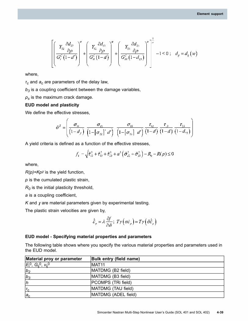
Element support
where,
τc and ac are parameters of the delay law,
b3 is a coupling coefficient between the damage variables,
ρs is the maximum crack damage.
EUD model and plasticityWe define the effective stresses,
A yield criteria is defined as a function of the effective stresses,
where,
R(p)=Kpɣ is the yield function,
p is the cumulated plastic strain,
R0 is the initial plasticity threshold,
a is a coupling coefficient,
K and ɣ are material parameters given by experimental testing.The plastic strain velocities are given by,
EUD model - Specifying material properties and parameters
The following table shows where you specify the various material properties and parameters used inthe EUD model.
Material proy or parameter Bulk entry (field name)Ei0, Gij0, νij0 MAT11b2 MATDMG (B2 field)b3 MATDMG (B3 field)h PCOMPS (TRi field)τc MATDMG (TAU field)ac MATDMG (ADEL field)
Simcenter Nastran Multi-Step Nonlinear User’s Guide (SOL 401 and SOL 402) 4-39
Element support

Chapter 4: Element support
Material proy or parameter Bulk entry (field name)dmax MATDMG (DMAX field)a MATDMG (A field)R0 MATDMG (LITK field)Κ MATDMG (BIGK field)Y MATDMG (EXPN field)ζ+ MATDMG (KSIT field)ζ- MATDMG (KSIC field)YdfT MATDMG (Y11LIMT field)YdfC MATDMG (Y11LIMC field)Y0 MATDMG (Y012 field)Yc MATDMG (YC12 field)K MATDMG (K field)ds MATDMG (DS field)GIC MATDMG (GIC field)GIIC MATDMG (GIIC field)GIIIC MATDMG (GIIIC field)ρs MATDMG (RO1 field)min(h,hc) MATDMG (HBAR field)ɑ MATDMG (ALPHA field)Controls if delay effect is usedbefore applying the maximumdamage.
MATDMG (USER field)
4.11 Chocking elements (SOL 401)Chocking element is a special type of axisymmetric element that is used to model regions in anaxisymmetric analysis that can carry a compressive hoop stress, but cannot carry a tensile hoopstress. You use chocking elements to model regions where the axisymmetric geometry is violated byregularly-spaced features like holes or keyways.
Chocking elements behave like axisymmetric elements when a copressive hoop stress is present,and behave like plane stress elements otherwise.
An example is the shrouding around the periphery of turbine blades in an aircraft engine.
4-40 Simcenter Nastran Multi-Step Nonlinear User’s Guide (SOL 401 and SOL 402)
Chapter 4: Element support

Element support
A generic turbine assembly is shown in the figure. You can see that the shroud is constructed fromdiscrete segments that are attached to each turbine blade. A small gap exists between each segment.If the combination of mechanical and thermal loads is such that these gaps close, the shroud cansustain a compressive hoop stress. To account for this behavior in an axisymmetric model, you canmesh the shroud cross section with chocking elements.
Tip
As a rule, only use chocking elements in combination with axisymmetric elements. A meshcomprised solely of chocking elements may lead to singularities, convergence issues, anderroneous results.
Gap status
An expression for the gap size at the end of a time step for each Gauss point is obtained as follows:
1. In the deformed configuration, the circumferential distance occupied by the chocking elementis given by
2πr – Ng
where N is the number of gaps, g is the gap size at the end of the iteration and r is the radiusat the end of the iteration.
2. Because εθ is an engineering strain, and engineering strains are based on undeformed lengths,the circumferential distance occupied by the chocking element in the deformed configurationis also given by
(1 + εθ) (2πr0 – Ng0)
where r0 is the initial radius and g0 is the initial gap size.
3. Equating the above terms for the circumferential distance occupied by the chocking element inthe deformed configuration and solving for the gap size at the end of the iteration yields
g = (1 / N) [2πr – (1 + εθ) (2πr0 – Ng0)]
Using the expression above for the gap size, the software calculates the gap status at each Gausspoint.
Simcenter Nastran Multi-Step Nonlinear User’s Guide (SOL 401 and SOL 402) 4-41
Element support
Chapter 4: Element support
Chocked status
At any Gauss point location where g ≤ 0, the location is considered chocked, and the contributionto the elemental stiffness matrix from that Gauss point is based on the axisymmetric formulation ofthe chocking element.
Unchocked status
At any Gauss point location where g > 0, the location is considered unchocked, and the contributionto the elemental stiffness matrix from that Gauss point is based on the axisymmetric formulation ofthe chocking element with the Eθ, νθr, and νθz elastic constants reduced by a factor of 1 x 10⁶.Doing so causes the element stiffness to be essentially identical to a plane stress formulation withσθ as the out-of-plane normal stress.
Large displacement on (LGDISP=1)
When large displacements are enabled, the software computes an updated gap status at the end ofeach time step. The resulting stiffness can then change from one time step to the next based onthe changing gap status and the deformed state of the model.
For applications of chocking elements like the turbine shroud, the mesh of chocking elements isconnected to axisymmetric elements. Because the stiffness in the radial direction for such a modelis relatively large, even when a positive gap exists, the incremental radial displacements that thesoftware calculates during the iterative solution are relatively small and the solution is able toconverge.
However, if the model is extremely compliant in the radial direction, the radial coordinates that thesoftware calculates to reformulate the stiffness may be negative, which is physically impossible.When the software detects a negative radial coordinate, it does not reformulate the stiffness matrixand it uses the initial circumferential distance for the deformed configuration at the next iteration.
To enable large displacements, specify PARAM,LGDISP,1.
Large displacement off (LGDISP=-1)
When large displacements are not enabled, you can use the parameter CHOCK on the NLCNTLGbulk entry to control the frequency of gap status updates.
When CHOCK=NO, a solution occurs for the first time step to determine the gap status at each Gausspoint. The software uses this chocked or unchocked status to recompute the stiffness. The resultingstiffness is then used for the rest of the solution, and the gap status is not reevaluated.
When CHOCK=YES (default), the software computes an updated gap status at the end of every timestep. The software uses this updated chocked or unchocked status to recompute the stiffness. Theresulting stiffness can change from one time step to the next based on the changing gap status, butnot on the deformed state of the model.
The CHOCK=YES option allows you to update the stiffness based on the chocking status, but withoutthe computation expense of running a large displacement analysis. This option is only appropriatewhen the changing geometry and stiffness updates that occur with LGDISP=1 are not significant.
PARAM,LGDISP,-1 is the default value for the LGDISP parameter.
4-42 Simcenter Nastran Multi-Step Nonlinear User’s Guide (SOL 401 and SOL 402)
Chapter 4: Element support

Element support
Note
The axisymmetric formulation of chocking elements sustains tensile, as well ascompressive hoop stress. Because the gap distance does not update when using theCHOCK=NO option, overly stiff results can occur for loadings that tend to increase thegap distance.
Surface tractions on chocking elements
Use the PLOADX1 bulk entry to apply surface tractions to the edges of chocking elements. When thesoftware calculates the equivalent grid point forces from the surface traction data on a PLOADX1bulk entry, it accounts for the presence of gaps.
For example, suppose you use a PLOADX1 bulk entry to apply a pressure along the edge of achocking element. If the edge is directed in the axial direction, the total force applied to the chockingelement over 2π radians is:
p (2πr – Ng) L
where p is the pressure, r is the radial coordinate of the edge, N is the number of gaps, g is the gapsize, and L is the length of the edge.
Chocking element types
Four elements support the chocking capability. They are:
• CCHOCK3 – A triangular chocking element
• CCHOCK4 – A quadrilateral chocking element
• CCHOCK6 – A triangular chocking element with midside nodes
• CCHOCK8 – A quadrilateral chocking element with midside nodes
All four chocking elements must reference the PCHOCK property bulk entry. On the PCHOCK bulkentry, you specify the material property for the chocking element and the number of gaps. You canspecify the initial gap thickness on either the PCHOCK bulk entry or on the chocking element bulkentries that reference the PCHOCK bulk entry. If the initial gap thickness is specified on both, thespecification on the chocking element bulk entry takes precedence. If the gap is of uniform thickness,use the GAPT field on the PCHOCK bulk entry to specify the gap thickness. If the gap thicknessvaries through the cross section, use the GAPi fields on the chocking element bulk entries, or use acombination of GAPT specifications and GAPi overrides, to specify the gap thickness.
To request gap results output, use the CKGAP case control command.
4.12 Cohesive elementsIn SOLs 401 and 402, you can use cohesive elements to model adhesively bonded interfaces. Theadvantages of cohesive elements over traditional glue connections in Simcenter Nastran are thatwith cohesive elements, you can account for:
• Compliance in the connection.
Simcenter Nastran Multi-Step Nonlinear User’s Guide (SOL 401 and SOL 402) 4-43
Element support

Chapter 4: Element support
• Damage in the material.
You can define cohesive elements with the CHEXCZ and CPENTCZ elements. You can definethese elements as occupying a solid volume or a planar area. To define the element geometrysuch that it occupies a planar area, define coincident grid points on each edge that connects thetop and bottom faces.
For example, to define the CPENTCZ element as a planar area, G1, G10, and G4 must have thesame coordinates. G1 is also included in the connectivity of an element that is part of the mesh onone side of the interface and G4 is also included in the connectivity of an element that is part of themesh on the other side of the interface. Mid-side grid points on edges that connect the top andbottom faces like G10 are exclusive to the cohesive element mesh.
CHEXCZ and CPENTCZ elements must reference a PSOLCZ property. With the PSOLCZ bulk entry,you reference the corresponding MAT1, MAT11, or MATCZ bulk entry, the material coordinate system,and, under certain circumstances, the thickness of the element.
There are three stiffness values associated with cohesive elements: K01 and K02 are the transverseshear stiffness; K03S is the out-of-plane normal stiffness. You specify these stiffness values asfollows:
• If the PSOLCZ bulk entry references a MAT1 bulk entry, Simcenter Nastran calculates thestiffness of the cohesive elements to be K01 = G / THICK, K02 = G / THICK, and K03S = E /THICK, where THICK is the value you specify in the THICK field of the PSOLCZ bulk entry.
• If the PSOLCZ bulk entry references a MAT11 bulk entry, Simcenter Nastran calculates thestiffness of the cohesive elements to be K01 = G13 / THICK, K02 = G23 / THICK, and K03S = E3/ THICK, where THICK is the value you specify in the THICK field of the PSOLCZ bulk entry.
• If the PSOLCZ bulk entry references a MATCZ bulk entry, you specify the stiffness directly inthe K01, K02, and K03S fields of the MATCZ bulk entry. For this case, the THICK field of thePSOLCZ bulk entry is ignored.
In all three cases, Simcenter Nastran does not use the physical thickness of cohesive elements asdefined by the geometric coordinates of the grids to determine the stiffness of the cohesive element.
You use the MATCZ bulk entry when you want to obtain material damage estimates. To activatedamage estimation, include PARAM,MATNL,1 in your input file. On the MATCZ bulk entry, specify thedamage estimation model. You can choose from the following options:
• In the polynomial model (the default), the Mode I, Mode II, and Mode III damage variables aretaken to be equal, and the damage is modeled as a function of thermodynamic force. Anevolution equation is used to estimate the damage.
• In the bi-triangular model, for Mode I, Mode II, and Mode III, the relationship between stress anddisplacement is modeled as bilinear.
• In the exponential model,for Mode I, Mode II, and Mode III, the relationship between stressand displacement is modeled as exponential.
Simcenter Nastran also does not use the physical thickness of cohesive elements as defined by thegeometric coordinates of the grids in damage calculations.
Results for cohesive elements are calculated at the corner grid points. The results include:
4-44 Simcenter Nastran Multi-Step Nonlinear User’s Guide (SOL 401 and SOL 402)
Chapter 4: Element support

Element support
• Damage values
• Surface tractions
• Relative displacements
To request result output for cohesive elements, use the CZRESULTS case control command.With the CZRESULTS case control command, you can request the damage for all three modes,components of the surface tractions, and components of the relative displacements. Relativedisplacement is defined as the displacement of the top surface of the cohesive element relativeto the bottom surface of the cohesive element.
Traction and relative displacement are both output into three components. The components areoutput in the material coordinate system relative to the deformed state. Tractions have units of forceper unit area. Relative deformation has units of length.
4.13 Crack simulation (SOL 401)You can compute and output the j-integral for a given crack geometry. This capability is onlysupported for SOL 401. The j-integral output can be used by third-party software like Zencrack toperform a fracture mechanics analysis.
• You can use the JINTEG case control command to control the computation and output of thej-integral. With the JINTEG case control command, you can direct the j-integral output to either.op2 or .f06 files.
For additional information, see the JINTEG case control command.
• The creation of the CRAKTP bulk entry. You can use the CRAKTP bulk entry to specifyinformation related to the crack tip.
For additional information, see the CRAKTP bulk entry in the Simcenter Nastran Quick ReferenceGuide.
• The creation of the VCEV bulk entry. You can use the VCEV bulk entry to define virtual cracktip extension vectors.
For additional information, see the VCEV bulk entry in the Simcenter Nastran Quick ReferenceGuide.
• The modification of the CHEXA bulk entry to allow for collapsed CHEXA element definition. Notethat the collapsed CHEXA element is not supported in a glue or contact region.
• The creation of the COLPHEXA parameter. You can allow collapsed CHEXA elements to bypassinput file checks with the COLPHEXA parameter. To do so, specify PARAM,COLPHEXA,YESin the bulk section of the input file.
Collapsed CHEXA elements
Any face of a CHEXA element can be collapsed to an edge. The edge of the collapsed facerepresents the crack front.
Figure 4-2 shows the connectivity for a standard CHEXA element.
Simcenter Nastran Multi-Step Nonlinear User’s Guide (SOL 401 and SOL 402) 4-45
Element support

Chapter 4: Element support
Figure 4-2. Standard CHEXA Element
Figure 4-3 shows the CHEXA element of Figure 4-2 with the G2–G14–G6–G18–G7–G15–G3–G10face collapsed so that the G2–G14–G6 edge and the G3–G15–G7 edge become the crackfront. Alternately, the G2–G14–G6–G18–G7–G15–G3–G10 face could be collapsed so that theG2–G10–G3 edge and the G6–G18–G7 edge would become the crack front.
Figure 4-3. Collapsed CHEXA Element
Two options are available for specifying a CHEXA element with a collapsed face:
• In Format 1, 15 unique grid IDs are specified in the 20 grid ID fields of the CHEXA bulk entry.Format 1 is typically used for elastic material models. With Format 1, mid-side grids can move tothe quarter-span locations closest to the crack front.
For the collapsed CHEXA element shown in Figure 4-3, the Format 1 specification is as follows:
1 2 3 4 5 6 7 8 9 10CHEXA EID PID G1 G2 G2 G4 G5 G6
G6 G8 G9 G2 G11 G12 G13 G14
4-46 Simcenter Nastran Multi-Step Nonlinear User’s Guide (SOL 401 and SOL 402)
Chapter 4: Element support

Element support
1 2 3 4 5 6 7 8 9 10
G14 G16 G17 G6 G19 G20
where the same grid ID is entered in the G2, G3, and G10 fields, another grid ID is entered inboth the G14 and G15 fields, and another grid ID is entered in the G6, G7, and G18 fields.
• In Format 2, 20 unique grid IDs are specified in the 20 grid ID fields of the CHEXA bulk entry.However, eight of the grid IDs do not have unique coordinates. Format 2 is typically used forelasto-plastic material models. With Format 2, mid-side grids remain at the mid-span locations.
For the collapsed CHEXA element shown in Figure 4-3, the Format 2 specification is as follows:
1 2 3 4 5 6 7 8 9 10CHEXA EID PID G1 G2 G3 G4 G5 G6
G7 G8 G9 G10 G11 G12 G13 G14
G15 G16 G17 G18 G19 G20
where the grids entered in the G2, G3, and G10 fields would share the same coordinates, thegrids entered in the G14 and G15 fields would share the same coordinates, and the grids enteredin the G6, G7, and G18 fields would share the same coordinates. Unlike Format 1 where grids inthe CHEXA element connectivity are merged, Format 2 does not merge coincident grids in theCHEXA element connectivity. Thus, these grids can move independently of one another.
4.14 Stress output coordinate systemSOLs 401 and 402 output stress and strain in the body-fixed material coordinate system for thefollowing elements, where the body-fixed material coordinate system is the material coordinatesystem relative to the deformed state.
• 3D solids elements CTETRA, CHEXA, CPENTA and CPYRAM
• Plane strain elements CPLSTN3, CPLSTN4, CPLSTN6, CPLSTN8
• Plane stress elements CPLSTS3, CPLSTS4, CPLSTS6, CPLSTS8
• Shell elements CTRIAR, CQUADR, CTRIA6, and CQUAD8 along with the CQUAD4 and CTRIA3which are automatically converted to CQUADR and CTRIAR elements.
The transformation matrix from the initial or the body-fixed material coordinate system to the basiccoordinate system is written to the TRMBU or TRMBD datablocks, respectively, for post processors.
3D solid, plane strain, and plane stress elements ouput options (SOL 401 only)
In SOL 401, the SYSTEM(627)=0 setting is available to optionally write the stress and strain outputfor the 3D solid, plane strain, and plane stress elements to the basic coordinate system.
• SYSTEM(627)=0 - SOL 401 outputs stress and strain on the 3D solid, plane strain, and planestress elements in the basic coordinate system.
• SYSTEM(627)=1 (Default) - SOL 401 outputs stress and strain on the 3D solid, plane strain, andplane stress elements in the body-fixed material coordinate system.
Simcenter Nastran Multi-Step Nonlinear User’s Guide (SOL 401 and SOL 402) 4-47
Element support

Chapter 4: Element support
The system cell 627 does not apply to the shell, beam, spring, or cohesive elements.
Shell, beam, spring, or cohesive elements output options
• For the shell elements CTRIAR, CQUADR, CTRIA6, and CQUAD8 along with the CQUAD4 andCTRIA3 elements that are automatically converted to CQUADR and CTRIAR elements, thestress, strain, and element force (shell resultants) are always output in the body-fixed materialcoordinate system.
• For the CBAR and CBEAM elements, the stress, strain, and element force (beam resultants)are always output in the body-fixed element coordinate system, where the body-fixed elementcoordinate system is the element coordinate system relative to the deformed state.
• Cohesive elements, the relative displacements, and tractions are always output in the body-fixedmaterial coordinate system.
4.15 Kinematic joints (SOL 402)Solution 402 supports kinematic joints and flexible sliders. Kinematic joints allow structural analysesof an assembly containing moving parts.
This capability lets you solve models such as aerostructures, helicopters, deployable structures inspace, gas turbines, and machine tools.
You can also use flexible slider joints to drive displacement of parts along beams, such as a modelof a track.
Kinematic joints
A kinematic joint connects two nodes. For some of the joints, you can define a third node foradditional spring or damper properties, or for driver loads.
4-48 Simcenter Nastran Multi-Step Nonlinear User’s Guide (SOL 401 and SOL 402)
Chapter 4: Element support

Element support
(1) Horizontal sliders; (2) Vertical sliders; (3) Rotating cylinder for swivel arm; (4) Rotatingcylinder for mill head
In the CJOINT bulk entry, you define the joint connectivity: a joint connects two nodes, N1 and N2.
In the PJOINT bulk entry, you define the joint type. Depending on the joint type, you can modeldifferent behaviors for the kinematic of the joint and you can constrain some DOFs:
Slider joints
Joint type Description
INLINE This joint constrains the 2nd node to slide along the straight line that joins bothnodes, and allows the relative rotations between the nodes.
SLIDER This joint constrains the 2nd node to slide along the straight line that joins bothnodes, but fixes the relative rotation between the nodes.
CYLDR This joint constrains the 2nd node to slide along the straight line that joins bothnodes and allows a relative rotation between the nodes along that axis.
SLIUNVThis joint constrains the 2nd node to slide along the straight line that joins bothnodes. A universal joint relation is introduced between the rotations of the twonodes.
SCREWThis joint acts as the CYLDR joint, but the relative rotation around andtranslation along the straight line that joins both nodes are related by the pitchproperty of the screw.
Simcenter Nastran Multi-Step Nonlinear User’s Guide (SOL 401 and SOL 402) 4-49
Element support

Chapter 4: Element support
Kinematic joints with coincident nodes
All the joints in the following table have two coincident nodes.
Joint type Description
REVOLUTE The joint constrains the nodes to rotate relative to each other along an axisthat the you define.
SPHERE This joint allows the relative rotation between the two nodes, but fixes theirrelative translation.
FIXED This joint introduces rigid links between the two nodes. The links can bereleased per DOF at a given time.
UNIVSL This joint acts as two combined REVOLUTE joints and designs a cardan shaft.
CONVEL A constant velocity joint is similar to a universal joint, except that a constantvelocity joint ensures a constant velocity through the joint's spin axis.
Options
Optionally, in the PJOINT bulk entry, you define the stiffness of the joint and add friction to thebehavior of the joint, while in the PJOINT2 bulk entry, you add a spring and/or damper behavior.
With the DRIVER bulk entry, you load the joint with a force or an imposed displacement for atranslational DOF. You load the joint with a torque or an imposed rotation for a rotational DOF
In the JRESULTS case control command, you set output requests for the joint.
With the JCON bulk entry, you can define time constraints on a joint. At a given time, you can fixor release the movement of the whole joint. For the FIXED joint, the links can be released perDOF at a given time.
Flexible sliders
The FLXSLI bulk entry lets you define flexible sliders. You set a list of nodes to follow a track madeof beams.
(1) nodes to be displaced along the beam elements, (2) beam elements, (3) slider elementsgenerated by the solver, (4) sensor node
You can define several slider types depending on how you want to control the relative rotations ofthe nodes around the track.
You can also define friction and, with a driver, you can impose a force or displacement on the slider.
When you set a driver, you can also request to output the relative displacement along the curvilinearabscissa of the track with the FLXRESULTS case control command.
4-50 Simcenter Nastran Multi-Step Nonlinear User’s Guide (SOL 401 and SOL 402)
Chapter 4: Element support

Element support
4.16 Formulation of isoparametric elementsIn the finite element method, parametric mapping is frequently used to map an irregular region into aregular one. The coordinate system used in the parametric mapping is a natural coordinate systemsuitable for the geometry. For instance, a natural coordinate system (ξ,η) is used for a quadrilateralsurface in which each corner node has an extremum value of +1 or -1 in ξ and η. Then, the geometryof the internal points of the finite element can be described in terms of the nodal coordinates by theparametric mapping. The mathematical expression for this parametric mapping or interpolation iscalled a shape function. The displacement field inside the element should also be interpolated interms of nodal displacements. The mapping is isoparametric if the same shape function is used tointerpolate the displacement field as well as the geometry. The merit of isoparametric mapping is thatthe displacement field is invariant to the orientation of the Cartesian coordinate system x and y.
Most of the elements are isoparametric elements, in which the shape functions are expressed interms of isoparametric coordinates. In what follows, derivations are shown for the isoparametriccoordinates, shape functions, element matrix describing the strain-displacement relations, volumeintegration for stiffness and mass matrices by Gauss quadrature, and element loads are derived fora tetrahedron element to illustrate element related operations.
4.16.1 Isoparametric coordinates
Cartesian coordinates are not convenient to describe the geometry or the displacement field of atetrahedron element. Let us introduce a set of volume coordinates (L1 L2 L3 L4), such that
as shown in the figure Volume Coordinates for Tetrahedron. The relation between volume andCartesian coordinates can be established for a linear tetrahedron (without midside nodes) as follows:
x = L1x1 + L2x2 + L3x3 +L4x4y = L1y1 + L2y2 + L3y3 +L4y4z = L1z1 + L2z2 + L3z3 +L4z41 = L1 + L2 + L3 +L4
Equation 4-15.It is obvious from Equation 4-15 that the shape functions are simply the volume coordinates, i.e.,
N1 = L1, N2 = L2, ..., etc.
Equation 4-16.because x = Σ Nixi.
Shape functions for the quadratic tetrahedron can be derived using Lagrangian interpolation. Theseare
N1 = (2L1 – 1)L1, etc. for corner nodes
and N5 = 4L1, L2, etc. for midside nodes.
Equation 4-17.
Simcenter Nastran Multi-Step Nonlinear User’s Guide (SOL 401 and SOL 402) 4-51
Element support

Chapter 4: Element support
Notice that these shape functions, Equations 4-16 and 4-17, satisfy element convergence criteria:integrability (Cn-1 continuity for n-th derivative) and completeness (no straining by a rigid body mode,constant strain condition, and continuous displacement field).
With the isoparametric element, the same shape functions are used to describe the displacementfield as well as the geometry, i.e.,
Equation 4-18.
The strains are calculated as
Equation 4-19.
where strain vector
Equation 4-20.
element matrix
Equation 4-21.
nodal displacement vector
Equation 4-22.
with
Equation 4-23.
4-52 Simcenter Nastran Multi-Step Nonlinear User’s Guide (SOL 401 and SOL 402)
Chapter 4: Element support

Element support
Equation 4-24.
Because the shape functions are defined in terms of local coordinates, a coordinate transformation isrequired to obtain global derivatives. Volume coordinates involve four coordinates (one of which isdependent), and the Jacobian matrix will become rectangular. To avoid this difficulty, let us introducelocal coordinates (ξ,η,ζ) as follows:
Equation 4-25.
Derivatives with respect to the local coordinates can be expressed in terms of global derivativesusing the chain rule, i.e.,
Equation 4-26.
where the Jacobian matrix is expressed in terms of shape functions as
Simcenter Nastran Multi-Step Nonlinear User’s Guide (SOL 401 and SOL 402) 4-53
Element support

Chapter 4: Element support
Equation 4-27.
This Jacobian matrix must be inverted to obtain global derivatives, from which the element matrix isformed. Notice that the determinant of the Jacobian matrix is called Jacobian which represents avolume change, i.e.,
Equation 4-28.
4.16.2 Shape functions
To make tetrahedron element compatible with other solid elements (HEXA and PENTA), deletionof any or.all of.the midside nodes is permitted. The shape functions are modified with Kronekerdeltas (δ5 - δ10) where
δi = 0 if the midside node i is deleted
= 1 if the midside node i is not deleted
The goal is to construct functions which are unity at the associated node and zero at all other nodes,regardless of any combination of deleted midside nodes, by the following scheme. At the corner nodes
At the midside nodes
Shape functions are identified as follows:
4-54 Simcenter Nastran Multi-Step Nonlinear User’s Guide (SOL 401 and SOL 402)
Chapter 4: Element support

Element support
Derivatives of the shape functions with respect to the local coordinates are obtained as follows:
Simcenter Nastran Multi-Step Nonlinear User’s Guide (SOL 401 and SOL 402) 4-55
Element support

Chapter 4: Element support
These shape functions and derivatives may be reduced to those for 4-noded and 10-nodedtetrahedron elements. It can be verified that, for any combination of deleted midside nodes, thereexist a condition
which satisfies the constant strain requirement.
4.16.3 Example element matrix
To illustrate the computational procedure, an element matrix for a linear tetrahedron (4-noded)element is explicitly derived here. The shape functions and the derivatives are tabulated below:
Node Ni δNi/δξ δNi/δη δNi/δς1 ξ 1 0 02 η 0 1 03 ς 0 0 14 1 – ξ – η – ς –1 -1 –1
Then the Jacobian matrix may be found as
where (xij = xi - xj) is used for convenience. Upon inverting the Jacobian matrix, we have
where
The global derivatives of the shape functions are
4-56 Simcenter Nastran Multi-Step Nonlinear User’s Guide (SOL 401 and SOL 402)
Chapter 4: Element support
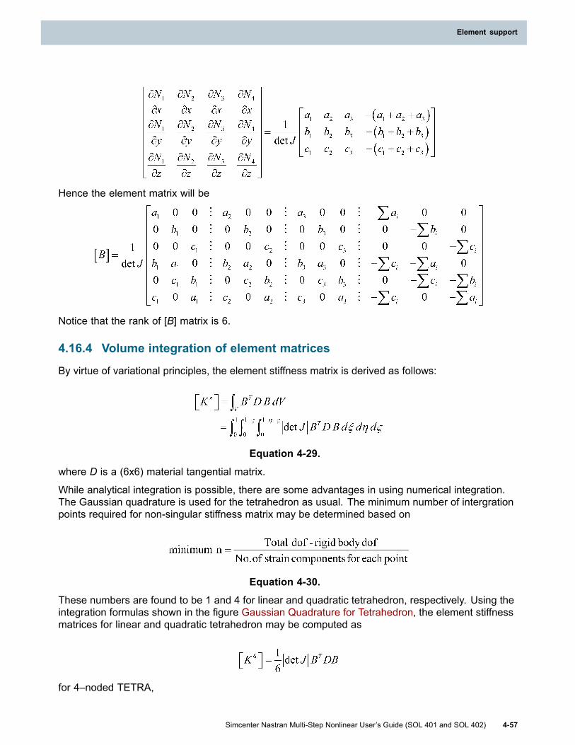
Element support
Hence the element matrix will be
Notice that the rank of [B] matrix is 6.
4.16.4 Volume integration of element matrices
By virtue of variational principles, the element stiffness matrix is derived as follows:
Equation 4-29.
where D is a (6x6) material tangential matrix.
While analytical integration is possible, there are some advantages in using numerical integration.The Gaussian quadrature is used for the tetrahedron as usual. The minimum number of intergrationpoints required for non-singular stiffness matrix may be determined based on
Equation 4-30.
These numbers are found to be 1 and 4 for linear and quadratic tetrahedron, respectively. Using theintegration formulas shown in the figure Gaussian Quadrature for Tetrahedron, the element stiffnessmatrices for linear and quadratic tetrahedron may be computed as
for 4–noded TETRA,
Simcenter Nastran Multi-Step Nonlinear User’s Guide (SOL 401 and SOL 402) 4-57
Element support

Chapter 4: Element support
for 5–10 noded TETRA,
Equation 4-31.
where the scaling factor 1/6 is introduced to compensate IJI =6x (Volume). One-point scheme shouldbe used for 4-noded tetrahedron (all the midside nodes deleted) and four-point scheme otherwise.
It is difficult to determine lumped masses when some of the midside nodes are deleted. However, theconsistent mass matrix may be obtained using the same shape functions, i.e.,
Equation 4-32.
where [Ň] = [N1I N2I ..... N10I], with I being (3x3) identity matrix. Again the Gaussian quadrature4-point formula is used to find
Equation 4-33.
Notice that 4-point scheme is to be used even for 4-noded tetrahedron. For computationalconvenience, the consistent mass may be converted to the lumped mass. One way to achieve this isto take the diagonal terms and scale them so that the total mass is preserved.
4.16.5 Element loads and equilibrium
Nodal forces are computed from the element stresses using element matrix, i.e.,
Equation 4-34.
The Gaussian integration is performed as
for 4-noded tetrahedron and
for (5-10)-noded tetrahedron.
Equation 4-35.
Thermal load is like an initial strain. Therefore, nodal forces due to thermal load are obtained by
4-58 Simcenter Nastran Multi-Step Nonlinear User’s Guide (SOL 401 and SOL 402)
Chapter 4: Element support

Element support
Equation 4-36.
where {εo}T = αΔT < 1 1 1 0 0 0 >. With anisotropic thermal properties, {εo}T becomes ΔT < α1,α2 ... α6 > in general.
The pressure load applied to any surface of the tetrahedron may be distributed to the grid points usingthe shape functions applicable to the 6-noded triangular element with removable midside nodes, i.e.,
Equation 4-37.
where {n} is a unit direction vector associated with a pressure (p) and
with I being (3 x 3) identity matrix. Shape functions (Ni’) are shown in the figure Shape Functions forPressure Load. Area integration should be performed using Gaussian quadrature formulas shown inthe figure Gaussian Quadrature for Pressure Load, i.e.,
Equation 4-38.
During the nonlinear iteration process, the equilibrium is not reached until convergence is achieved.The equilibrium is sought in the global level when the residual load R approaches zero. The residualload vector is defined as
Equation 4-39.
where {P} is the applied load vector including the thermal load and Σ implies assemblage in the globalcoordinate system (coordinate transformation required).
4.16.6 Element coordinates
The element coordinate system for the tetrahedron element is defined with the initial elementgeometry such that
• The origin is at the first grid point in the connectivity, G1.
• The x-axis is determined by connecting the origin G1 to node G2, i.e.,
Simcenter Nastran Multi-Step Nonlinear User’s Guide (SOL 401 and SOL 402) 4-59
Element support

Chapter 4: Element support
Equation 4-40.
• The y-axis is determined by orthonormalization (Gram-Schmidt process) of the edge direction(V13) with respect to x-axis,
Equation 4-41.
• The z-axis is orthogonal to x and y according to the right-hand rule, i.e.,
Then, the transformation from element coordinates to the basic coordinates is simply
Equation 4-42.
where
Equation 4-43.
and < xe, ye, ze > Tbasic is the position vector of the element coordinate system with respect to thebasic coordinate system. Notice that [Tbe] is an orthogonal matrix, i.e.,
4.16.7 Stress data recovery
In case of linear analysis, the stresses at the integration point are recovered as
Equation 4-44.
4-60 Simcenter Nastran Multi-Step Nonlinear User’s Guide (SOL 401 and SOL 402)
Chapter 4: Element support

Element support
with
where {σ}, [B], {u} and {α} are defined in the element coordinate system, and the shape function{Ni} interpolates Gauss point temperatures from the nodal temperatures. In case of nonlinearanalysis, stresses are computed again upon convergence, starting from the last converged state (lastconverged solution of σ and u), i.e.,
Given {σold} and
Equation 4-45.
with
the nonlinear material routine computes updated stresses {σnew}, which are stored in ESTNL.
To output grid point stresses, the stresses, the integration points must be extrapolated to the nodalpoints. A linear extrapolation can be applied using stresses at the element c.g. and the corner Gausspoint associated with a grid point. For a tetrahedron, referring to Figure 4-5,
Equation 4-46.
where
This yields
Equation 4-47.
In matrix form for all the grid points in the element
Simcenter Nastran Multi-Step Nonlinear User’s Guide (SOL 401 and SOL 402) 4-61
Element support

Chapter 4: Element support
Equation 4-48.
where
This process must be operated on every component of stress vector. No extrapolation is requiredfor 1-point integration.
4-62 Simcenter Nastran Multi-Step Nonlinear User’s Guide (SOL 401 and SOL 402)
Chapter 4: Element support

Element support
Figure 4-4. Volume Coordinates for Tetrahedron
Simcenter Nastran Multi-Step Nonlinear User’s Guide (SOL 401 and SOL 402) 4-63
Element support

Chapter 4: Element support
Figure 4-5. Gaussian Quadrature for Tetrahedron
4-64 Simcenter Nastran Multi-Step Nonlinear User’s Guide (SOL 401 and SOL 402)
Chapter 4: Element support
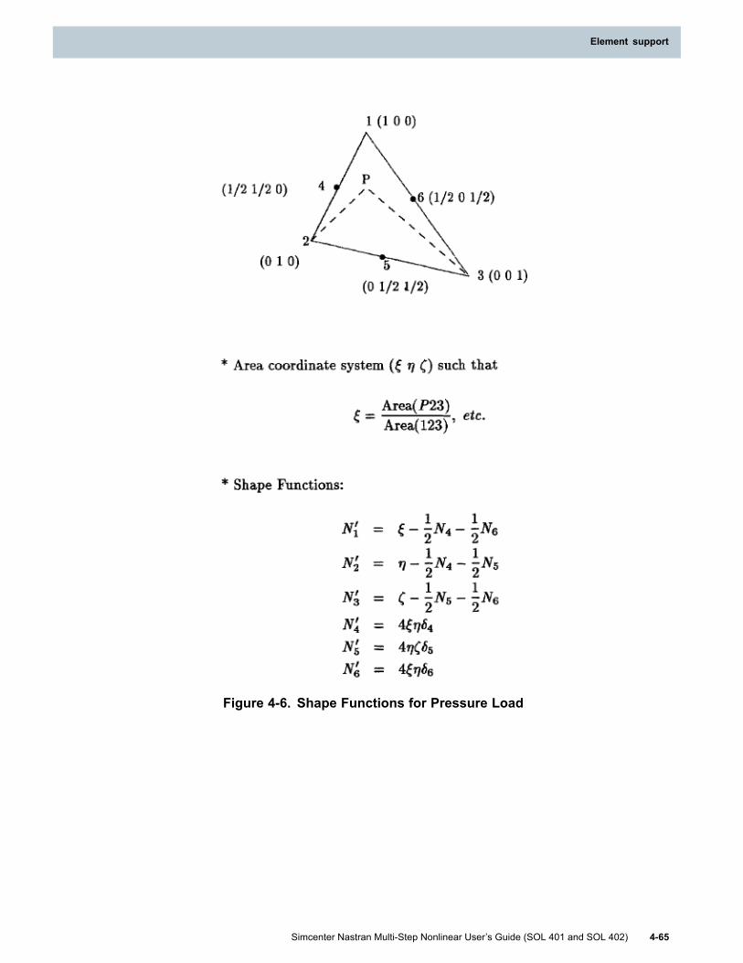
Element support
Figure 4-6. Shape Functions for Pressure Load
Simcenter Nastran Multi-Step Nonlinear User’s Guide (SOL 401 and SOL 402) 4-65
Element support

Chapter 4: Element support
Figure 4-7. Gaussian Quadrature for Pressure Load
4.17 Kinematic joints (SOL 402)Solution 402 supports kinematic joints and flexible sliders. Kinematic joints allow structural analysesof an assembly containing moving parts.
This capability lets you solve models such as aerostructures, helicopters, deployable structures inspace, gas turbines, and machine tools.
You can also use flexible slider joints to drive displacement of parts along beams, such as a modelof a track.
Kinematic joints
A kinematic joint connects two nodes. For some of the joints, you can define a third node foradditional spring or damper properties, or for driver loads.
4-66 Simcenter Nastran Multi-Step Nonlinear User’s Guide (SOL 401 and SOL 402)
Chapter 4: Element support
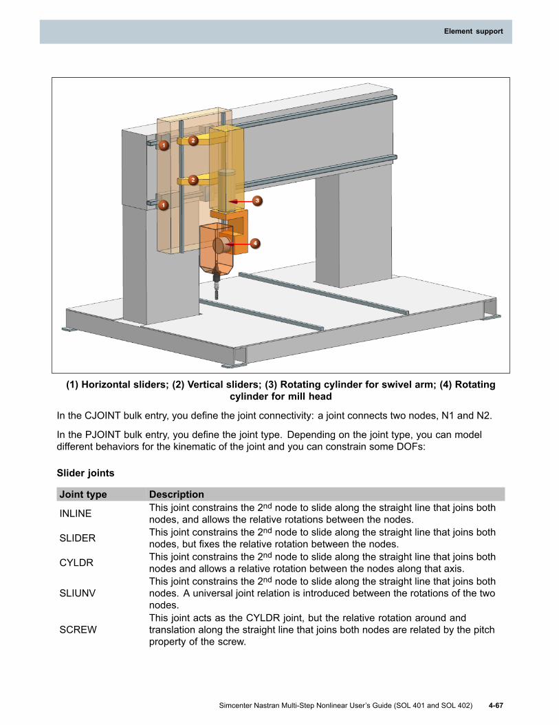
Element support
(1) Horizontal sliders; (2) Vertical sliders; (3) Rotating cylinder for swivel arm; (4) Rotatingcylinder for mill head
In the CJOINT bulk entry, you define the joint connectivity: a joint connects two nodes, N1 and N2.
In the PJOINT bulk entry, you define the joint type. Depending on the joint type, you can modeldifferent behaviors for the kinematic of the joint and you can constrain some DOFs:
Slider joints
Joint type Description
INLINE This joint constrains the 2nd node to slide along the straight line that joins bothnodes, and allows the relative rotations between the nodes.
SLIDER This joint constrains the 2nd node to slide along the straight line that joins bothnodes, but fixes the relative rotation between the nodes.
CYLDR This joint constrains the 2nd node to slide along the straight line that joins bothnodes and allows a relative rotation between the nodes along that axis.
SLIUNVThis joint constrains the 2nd node to slide along the straight line that joins bothnodes. A universal joint relation is introduced between the rotations of the twonodes.
SCREWThis joint acts as the CYLDR joint, but the relative rotation around andtranslation along the straight line that joins both nodes are related by the pitchproperty of the screw.
Simcenter Nastran Multi-Step Nonlinear User’s Guide (SOL 401 and SOL 402) 4-67
Element support

Chapter 4: Element support
Kinematic joints with coincident nodes
All the joints in the following table have two coincident nodes.
Joint type Description
REVOLUTE The joint constrains the nodes to rotate relative to each other along an axisthat the you define.
SPHERE This joint allows the relative rotation between the two nodes, but fixes theirrelative translation.
FIXED This joint introduces rigid links between the two nodes. The links can bereleased per DOF at a given time.
UNIVSL This joint acts as two combined REVOLUTE joints and designs a cardan shaft.
CONVEL A constant velocity joint is similar to a universal joint, except that a constantvelocity joint ensures a constant velocity through the joint's spin axis.
Options
Optionally, in the PJOINT bulk entry, you define the stiffness of the joint and add friction to thebehavior of the joint, while in the PJOINT2 bulk entry, you add a spring and/or damper behavior.
With the DRIVER bulk entry, you load the joint with a force or an imposed displacement for atranslational DOF. You load the joint with a torque or an imposed rotation for a rotational DOF
In the JRESULTS case control command, you set output requests for the joint.
With the JCON bulk entry, you can define time constraints on a joint. At a given time, you can fixor release the movement of the whole joint. For the FIXED joint, the links can be released perDOF at a given time.
Flexible sliders
The FLXSLI bulk entry lets you define flexible sliders. You set a list of nodes to follow a track madeof beams.
(1) nodes to be displaced along the beam elements, (2) beam elements, (3) slider elementsgenerated by the solver, (4) sensor node
You can define several slider types depending on how you want to control the relative rotations ofthe nodes around the track.
You can also define friction and, with a driver, you can impose a force or displacement on the slider.
When you set a driver, you can also request to output the relative displacement along the curvilinearabscissa of the track with the FLXRESULTS case control command.
4-68 Simcenter Nastran Multi-Step Nonlinear User’s Guide (SOL 401 and SOL 402)
Chapter 4: Element support

Chapter 5: Material support
5.1 Material overview
Material type support (SOLs 401 and 402)
• The MAT1 and MATT1 (temperature dependent) bulk entries define isotropic materials.
• The MAT2 and MATT2 (temperature dependent) bulk entries define anisotropic materials forshell elements.
• The MAT8 and MATT8 (temperature dependent) bulk entries define orthotropic materials forshell elements.
• The MAT3 and MATT3 (temperature dependent) bulk entries define orthotropic materials.
• The MAT9 and MATT9 (temperature dependent) bulk entries define anisotropic materials.
• The MAT11 and MATT11 (temperature dependent) bulk entries define orthotropic materials.
• The MATCZ bulk entry defines material properties for cohesive elements.
• The MATDMG bulk entry defines properties for progressive ply failure.
• The MATFT bulk entry defines the failure theory allowables for both shell and solid composites.
• The MPLAS bulk entry defines plastic material data.
• SOL 401 supports a nonlinear elastic material for the 3D solid, plane stress, plane strain,generalized plane strain, axisymmetric, chocking, and shell elements.
• Plastic and creep materials can optionally be assigned to the following elements: shell, 3Dsolid, axisymmetric, plane stress, plane strain, CBAR, and CBEAM. You can enable one or bothplasticity/creep in all subcases or in specific subcases.
The MATCRP and CREEP bulk entries define creep materials and properties.
You can enable one or both plasticity/creep in all subcases or in specific subcases.
• The MUMAT bulk entry defines the material properties for the user defined material subroutine.
For more information, see User defined materials.
• The MATSR specifies strain-rate dependent properties for use with a MATS1 entry.
• SOL 401 supports externally constructed, user-defined creep models.
Simcenter Nastran Multi-Step Nonlinear User’s Guide (SOL 401 and SOL 402) 5-1

Chapter 5: Material support
Material type support (SOL 402)
• The MATHE and MATHOP bulk entries define hyperelastic materials.
o The MATHEM bulk entry adds the Mullins effects to the MATHE material.
o The MATHEV bulk entry adds viscoplastic effects to the MATHE material.
• The MATSR specifies strain-rate dependent properties for use with a MATS1 entry.
• The MATTC bulk entry specifies temperature-dependent creep coefficients on CREEP entryfields using TABLEM1 entries.
For more information, see Hyperelastic materials (SOL 402).
5.2 Plasticity analysisYou can perform a plasticity analysis in SOLs 401 and 402. The constitutive model is a standardelastic-plastic model that allows for bilinear and multilinear stress-strain curve representations. Formultilinear representations, tabular data is used to define the stress-strain curve. You can specifythat the strain values in the tabular data are either total strain or plastic strain. You can also definematerial properties as temperature-dependent. At present, the von Mises yield criterion is the onlyyield criterion that is supported.
For bilinear stress-strain representations, you can select either isotropic, kinematic, or combinedhardening. For multilinear stress-strain representations, isotropic hardening is the only hardening ruleavailable.
You can selectively enable and disable plasticity effects in subcases. If plasticity-enabled subcasesare sequentially dependent, the plasticity state variables at the end of one subcase are used asthe plasticity state variables at the beginning of the next subcase. If a plasticity-disabled subcaseis placed between plasticity-enabled subcases, and the subcases are all sequentially dependent,the plasticity state variables at the end of the preceding plasticity-enabled subcase are used as theplasticity state variables at the beginning of the later plasticity-enabled subcase.
However, with the exception of special situations, we recommend you avoid placing a sequentiallydependent plasticity-disabled subcase after a plasticity-enabled subcase. Doing so eliminates thepossibility that the analysis does not account for changes to the plasticity state variables that mightresult from the loading in the plasticity-disabled subcase.
Creep analysis is also supported in SOLs 401 and 402. You can enable one or both plasticity/creep inall subcases, or you can enable one or both in specific subcases.
For more information about creep analysis, see Support for creep analysis.
User interface
• The MATNL parameter. With the MATNL parameter, you can globally switch the plasticityanalysis capability on or off.
• For SOL 401, the PLASTIC parameter is available on the NLCNTL bulk entry to optionally turn offthe plasticity capability in a subcase.
For SOL 402, you use the same parameter but in the NLCNTL2 bulk entry.
5-2 Simcenter Nastran Multi-Step Nonlinear User’s Guide (SOL 401 and SOL 402)
Chapter 5: Material support

Material support
• The MATS1 bulk entry allows you to define stress versus plastic strain tabular data.
To activate the plasticity analysis capability in SOLs 401 or 402, do the following:
1. Reference both the MAT1 and MATS1 bulk entries in the regions where plasticity occurs.
2. Specify PARAM,MATNL,1.
3. Include a NLCNTL case control command that points to a NLCNTL/NLCNTL2 bulk entry.
4. On the NLCNTL/NLCNTL2 bulk entry, specify any applicable parameters.
If your input file contains subcases, and you want to include the effects of plasticity in specificsubcases, but not others, you have two options.
Option 1: Use a global NLCNTL case control command
1. Specify PARAM,MATNL,1.
2. Include a NLCNTL case control command above the subcases that points to a NLCNTL/NLCNTL2bulk entry.
3. On the NLCNTL/NLCNTL2 bulk entry, specify the applicable parameters.
4. In the subcases from which you want to disable the plasticity analysis capability, include aNLCNTL case control command that points to a NLCNTL/NLCNTL2 bulk entry.
5. On the NLCNTL/NCLNTL2 bulk entry, specify the following:
• "PLASTIC" in a PARAMi field.
• "NO" in the corresponding VALUEi field.
Option 2: Include NLCNTL case control commands in every subcase
1. Specify PARAM,MATNL,1.
2. Include NLCNTL case control commands in each subcase. Multiple NLCNTL case controlcommands can point to a single NLCNTL/NLCNTL2 bulk entry.
3. In subcases in which you want to enable the plasticity analysis capability, point the NLCNTL casecontrol command to a NLCNTL/NLCNTL2 bulk entry with the applicable parameters specified.
4. In subcases in which you want to disable the plasticity analysis capability, point the NLCNTL casecontrol command to a NLCNTL/NLCNTL2 bulk entry with the following specified:
• "PLASTIC" in a PARAMi field.
• "NO" in the corresponding VALUEi field.
The property bulk entry referenced by all non-rigid elements must reference a MAT1 bulk entry anda MATS1 bulk entry that have the same material identification number. If the properties on theMAT1 bulk entry are temperature-dependent, include a MATT1 bulk entry with the same materialidentification number.
Simcenter Nastran Multi-Step Nonlinear User’s Guide (SOL 401 and SOL 402) 5-3
Material support

Chapter 5: Material support
On the MATS1 bulk entry, specify TYPE = “PLASTIC” or “PLSTRN” to select the strain type in tabulardata used to describe a multilinear stress-strain curve. Specify TYPE = “PLASTIC” if you want touse total strains. Specify TYPE = “PLSTRN” if you want to use plastic strains. Total and plasticstrains are related as follows:
where
To describe a bilinear stress-strain curve, specify either TYPE = “PLASTIC” or “PLSTRN” and enterthe work hardening slope, H, directly.
For additional information, see the MATS1 bulk entry in the Simcenter Nastran Quick ReferenceGuide.
Time step control
Unlike creep analysis, there is no adaptive time stepping for plasticity analysis. The time steps aredefined directly by the solution times. To define solution times for the plasticity analysis, include aTSTEP case control command in your input file that points to a TSTEP1 bulk entry. On the TSTEP1bulk entry, specify the solution times and the solution times you want results output.
5.3 Strain rate-dependent plasticitySOLs 401 and 402 support a strain rate-dependent plasticity material model. This material modelrepresents the hardening and the resulting increasing yield stress that occurs as the strain rateincreases.
You have two options to define the strain rate-dependent plasticity. For either option described below,in the regions of your model where you expect strain rate plasticity to occur, you will reference a MAT1entry, a MATS1 entry, and a MATSR entry, all with the same ID.
• Option 1: Static stress scalingThis option scales the static stress found from an elastic-plastic material defined with theMATS1 entry. The elastic-plastic material definition can also reference temperature dependentstress-strain data from the MATS1 entry.
You will define two constants on the MATSR bulk entry that are used in the plastic strain ratescaling function below.
The software determines the current static yield stress σstat using the elastic-plastic materialdefinition. The static yield stress value is then scaled using the following strain-rate scalingfunction.
where is the current equivalent plastic strain rate, D is a constant defined with the TSRATEfield on the MATSR entry, and P is a constant defined with the BVALUE field on the MATSR entry.
5-4 Simcenter Nastran Multi-Step Nonlinear User’s Guide (SOL 401 and SOL 402)
Chapter 5: Material support
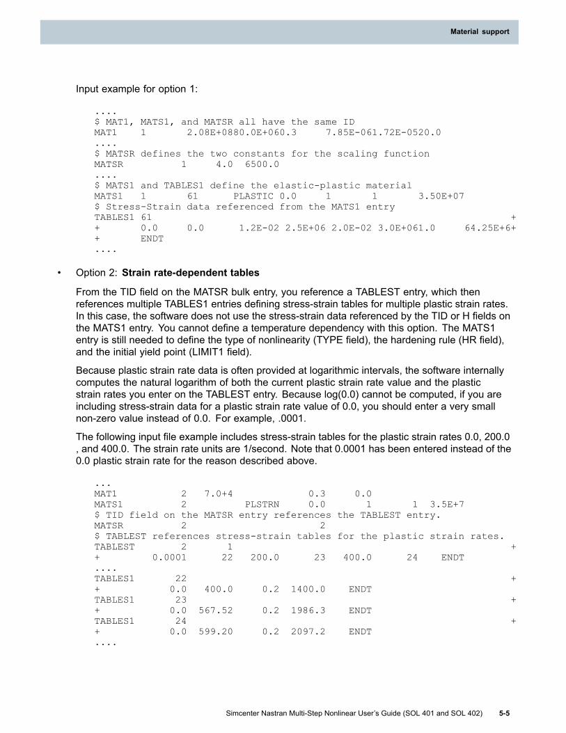
Material support
Input example for option 1:
....$ MAT1, MATS1, and MATSR all have the same IDMAT1 1 2.08E+0880.0E+060.3 7.85E-061.72E-0520.0....$ MATSR defines the two constants for the scaling functionMATSR 1 4.0 6500.0....$ MATS1 and TABLES1 define the elastic-plastic materialMATS1 1 61 PLASTIC 0.0 1 1 3.50E+07$ Stress-Strain data referenced from the MATS1 entryTABLES1 61 ++ 0.0 0.0 1.2E-02 2.5E+06 2.0E-02 3.0E+061.0 64.25E+6++ ENDT....
• Option 2: Strain rate-dependent tables
From the TID field on the MATSR bulk entry, you reference a TABLEST entry, which thenreferences multiple TABLES1 entries defining stress-strain tables for multiple plastic strain rates.In this case, the software does not use the stress-strain data referenced by the TID or H fields onthe MATS1 entry. You cannot define a temperature dependency with this option. The MATS1entry is still needed to define the type of nonlinearity (TYPE field), the hardening rule (HR field),and the initial yield point (LIMIT1 field).
Because plastic strain rate data is often provided at logarithmic intervals, the software internallycomputes the natural logarithm of both the current plastic strain rate value and the plasticstrain rates you enter on the TABLEST entry. Because log(0.0) cannot be computed, if you areincluding stress-strain data for a plastic strain rate value of 0.0, you should enter a very smallnon-zero value instead of 0.0. For example, .0001.
The following input file example includes stress-strain tables for the plastic strain rates 0.0, 200.0, and 400.0. The strain rate units are 1/second. Note that 0.0001 has been entered instead of the0.0 plastic strain rate for the reason described above.
...MAT1 2 7.0+4 0.3 0.0MATS1 2 PLSTRN 0.0 1 1 3.5E+7$ TID field on the MATSR entry references the TABLEST entry.MATSR 2 2$ TABLEST references stress-strain tables for the plastic strain rates.TABLEST 2 1 ++ 0.0001 22 200.0 23 400.0 24 ENDT....TABLES1 22 ++ 0.0 400.0 0.2 1400.0 ENDTTABLES1 23 ++ 0.0 567.52 0.2 1986.3 ENDTTABLES1 24 ++ 0.0 599.20 0.2 2097.2 ENDT....
Simcenter Nastran Multi-Step Nonlinear User’s Guide (SOL 401 and SOL 402) 5-5
Material support

Chapter 5: Material support
5.4 Cast iron plasticity SOLs 401 and 402SOLs 401 and 402 support the gray cast iron plasticity material model. Gray cast iron has thefollowing characteristics.
• In tension, it is brittle as a result of the graphite flakes in the microstructure that act as stressconcentrators resulting in reduced yield strength.
In compression, the effect of the graphite flakes is less significant, and the ductile response isthe same as most steels. The compressive yield stress can be three (or more) times largerthan the tensile yield stress.
• The elastic properties are the same under tension and compression, and are defined on a MAT1entry.
• In tension, it has an inelastic (plastic) volume change. As a result, you must define a plasticPoisson's ratio in tension, which is the absolute value of the ratio of the transverse to thelongitudinal plastic strain under uniaxial tension.
In compression, the software assumes no inelastic volume change (incompressible, Poisson'sratio = 0.5).
• It has different hardening and flow behavior in tension and compression.
In tension, the software uses a pressure-dependent yield surface with a non-associated flow rule.
In compression, the software uses the von Mises yield condition with an associated flow rule.
Input summary
The MPLAS bulk entry is available to define the plastic material data.
You define the elastic material data on the MAT1 entry, which has the same ID as the MPLAS entry.
The MPLAS format includes specific rows to define yield function data and hardening rule data.
MPLAS format for gray cast iron
1 2 3 4 5 6 7 8 9 10MPLAS MID Name/Descriptor
"YIELD" GCIRON"ISOH" "TABULAR" TID Tension "T" "PLS" "TRUE" NUPL
TIDCompression "C" "PLS" "TRUE"
• Because there is different behavior in tension and compression for the gray cast iron material,you must define an isotropic hardening data row for both tension data and compression. Field 5in these rows designates the data row as tension ("T") or compression ("C").
• The stress-strain data referenced from field 4 must be true (Cauchy) measures. The Xi, Yi datadefined on the TABLES1 entry must be stress-plastic strain, with the data beginning at the yieldpoint (X1=plastic strain at the yield point=0.0, Y1=yield stress).
• You must define the plastic Poisson's ratio in field 9 (NUPL) on the tension data row.
5-6 Simcenter Nastran Multi-Step Nonlinear User’s Guide (SOL 401 and SOL 402)
Chapter 5: Material support

Material support
• For all fields with character inputs, the text shown in quotes are the only supported values. Youmust define this text. See the MPLAS bulk entry in the Quick Reference Guide for the definitionof these fields.
• The second hardening row must have fields 2 and 3 blank, as shown in the format above.
Equations for gray cast iron material• Yield surfaces
Tension:
Compression:
where q, p, and r are stress invariants:
is the von Mises equivalent stress,
is the equivalent pressure stress,
is the third invariant of the deviatoric stress tensor,
is the identity tensor
is the stress deviator,
is the Cauchy stress.
The quantity results from the combination of q and r, and is defined as the angle of thetension yield surface in the meridional plane for the stress state.
• Flow rule
where in tension,
Simcenter Nastran Multi-Step Nonlinear User’s Guide (SOL 401 and SOL 402) 5-7
Material support

Chapter 5: Material support
and in compression,
where,
• Hardening rules
Tension:
Compression:
• Constitutive model
5.5 Overview of PlasticityFor plasticity in SOLs 401 and 402 include a von Mises yield function with an associated flow rule.Available options include isotropic hardening, kinematic hardening, and combined hardening. TheZiegler-Prager hardening rules are available for kinematic and combined hardening.
The plasticity model must also be calibrated with uniaxial stress-strain data. The strain informationmust be in the unitless form of length/length. Classical plasticity models include the following threefundamental ingredients.
1. A yield function or yield criterion defines the limit of elastic behavior for a general state of stress.
The yield function may be thought of as a surface in a six dimensional stress space. It dividesthe stress space into two regions. Points inside the yield surface are characterized by elasticstress-strain behavior while stress states on the yield surface are at the limit of elastic behavior.The yield function may be written as a function of stress and a hardening parameter k.
The von Mises yield function for an isotropic hardening material may be stated as:
5-8 Simcenter Nastran Multi-Step Nonlinear User’s Guide (SOL 401 and SOL 402)
Chapter 5: Material support

Material support
J2 is the second invariant of the deviatoric stress tensor. The deviatoric stresses, sij, are given by:
where σm is the mean or average normal stress, and δij is the Kronecker delta.
Isotropic hardening assumes that the uniaxial yield stress, σy, is a function of plastic straining.
For kinematic or combined hardening, the von Mises yield function is
J 2 is the second invariant of the shift stress that is defined as the deviatoric stress minus theback stress. The back stress may also be thought of as the position of the center of the yieldsurface in the six-dimensional stress space. For initially isotropic materials, the back stresstensor components are initially zero.
2. A flow rule determines the relative magnitudes of the components of the plastic strain incrementtensor.
The software uses an associated flow rule in which the plastic potential function, g, is the sameas the yield function, f, and the components of the plastic strain increment are given by:
In vector form, for the von Mises yield surface with kinematic hardening, the plastic flow vector isgiven by:
For isotropic hardening, this equation reduces to the well-known Prandtl-Reuss equations.
3. A hardening rule defines the changes in the yield function as a result of plastic straining.
Isotropic Hardening
Simcenter Nastran Multi-Step Nonlinear User’s Guide (SOL 401 and SOL 402) 5-9
Material support

Chapter 5: Material support
When you select isotropic hardening, the software uses a piece-wise linear stress-strain curve.The isotropic hardening assumption isn't very realistic for most materials subjected to cyclicloading. However, it is relatively simple and efficient.
Isotropic hardening assumes that the yield surface expands uniformly as a result of plasticstraining. This assumption is achieved by making the yield stress a function of the integratedeffective plastic strain increments, which for a von Mises material is:
The slope of the stress plastic strain curve, Ep, is called the plastic modulus. It can be obtained fromthe uniaxial stress-strain curve and is defined by:
For a von Mises material, the effective stress is given by:
Kinematic Hardening
When you select kinematic hardening, the software assumes a bilinear stress-strain curve. If thematerial database contains a multilinear representation, only the yield point and the tangent modulusof the first segment beyond the yield point are used to characterize the stress-strain behavior.
Kinematic hardening assumes that the yield surface translates in the stress space but doesn't changesize or shape. The yield stress, σy, doesn't change, but the back stress, αij, is a function of plasticstraining. The Ziegler-Prager kinematic hardening is one of the most widely used models. This modelassumes that the back stress increment is in the direction of the stress minus the back stress.
The factor, dμ, depends on the plastic strain history.
Ziegler-Prager Combined Kinematic Isotropic Hardening
When you select combined kinematic isotropic hardening, the software assumes a bilinearstress-strain curve. If the material database contains a multilinear representation, only the yieldpoint and the tangent modulus of the first segment beyond the yield point are used to characterizethe stress-strain behavior.
Combined hardening assumes that the yield surface both expands and translates in the stress space.The plastic strain increment is composed of two components shown in the following equations:
5-10 Simcenter Nastran Multi-Step Nonlinear User’s Guide (SOL 401 and SOL 402)
Chapter 5: Material support
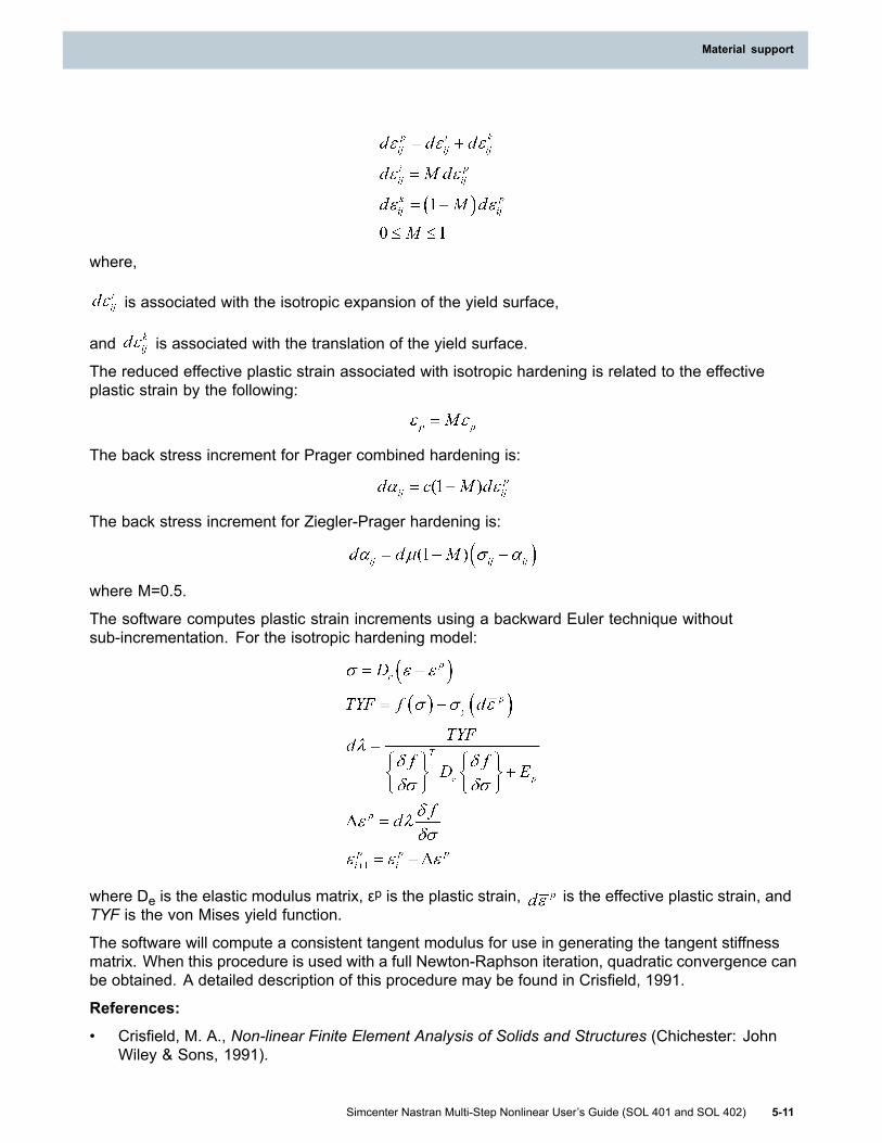
Material support
where,
is associated with the isotropic expansion of the yield surface,
and is associated with the translation of the yield surface.
The reduced effective plastic strain associated with isotropic hardening is related to the effectiveplastic strain by the following:
The back stress increment for Prager combined hardening is:
The back stress increment for Ziegler-Prager hardening is:
where M=0.5.
The software computes plastic strain increments using a backward Euler technique withoutsub-incrementation. For the isotropic hardening model:
where De is the elastic modulus matrix, εp is the plastic strain, is the effective plastic strain, andTYF is the von Mises yield function.
The software will compute a consistent tangent modulus for use in generating the tangent stiffnessmatrix. When this procedure is used with a full Newton-Raphson iteration, quadratic convergence canbe obtained. A detailed description of this procedure may be found in Crisfield, 1991.
References:
• Crisfield, M. A., Non-linear Finite Element Analysis of Solids and Structures (Chichester: JohnWiley & Sons, 1991).
Simcenter Nastran Multi-Step Nonlinear User’s Guide (SOL 401 and SOL 402) 5-11
Material support
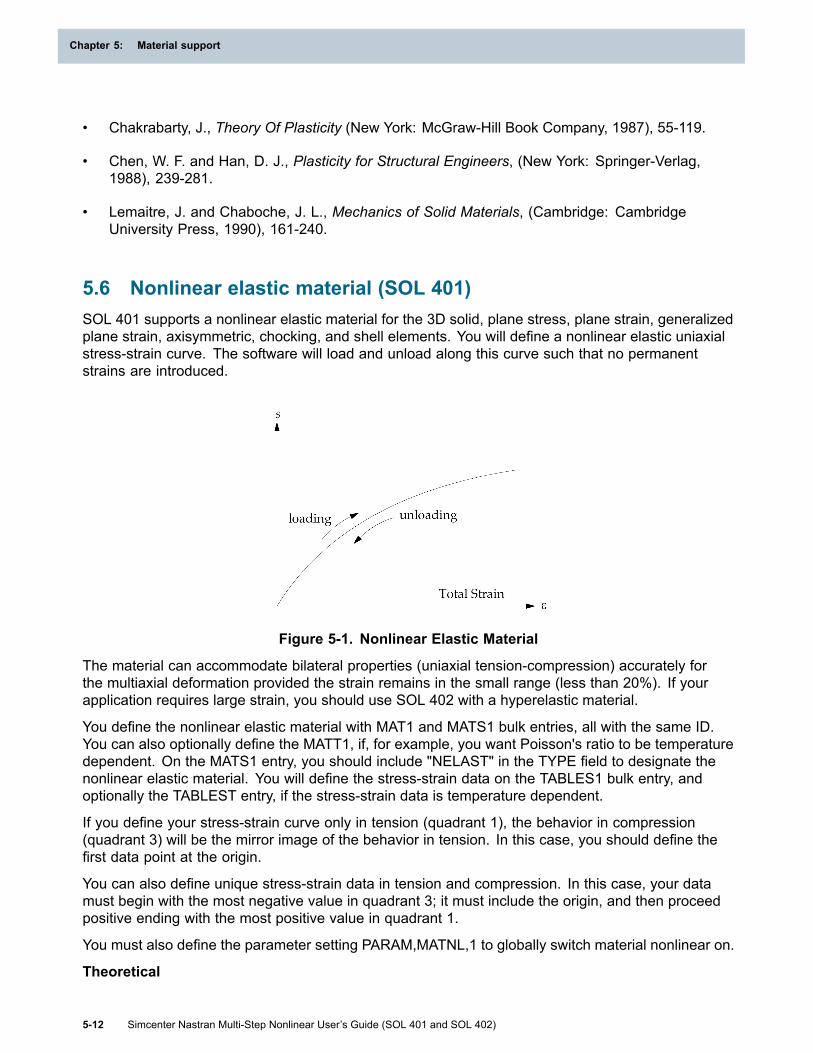
Chapter 5: Material support
• Chakrabarty, J., Theory Of Plasticity (New York: McGraw-Hill Book Company, 1987), 55-119.
• Chen, W. F. and Han, D. J., Plasticity for Structural Engineers, (New York: Springer-Verlag,1988), 239-281.
• Lemaitre, J. and Chaboche, J. L., Mechanics of Solid Materials, (Cambridge: CambridgeUniversity Press, 1990), 161-240.
5.6 Nonlinear elastic material (SOL 401)SOL 401 supports a nonlinear elastic material for the 3D solid, plane stress, plane strain, generalizedplane strain, axisymmetric, chocking, and shell elements. You will define a nonlinear elastic uniaxialstress-strain curve. The software will load and unload along this curve such that no permanentstrains are introduced.
Figure 5-1. Nonlinear Elastic Material
The material can accommodate bilateral properties (uniaxial tension-compression) accurately forthe multiaxial deformation provided the strain remains in the small range (less than 20%). If yourapplication requires large strain, you should use SOL 402 with a hyperelastic material.
You define the nonlinear elastic material with MAT1 and MATS1 bulk entries, all with the same ID.You can also optionally define the MATT1, if, for example, you want Poisson's ratio to be temperaturedependent. On the MATS1 entry, you should include "NELAST" in the TYPE field to designate thenonlinear elastic material. You will define the stress-strain data on the TABLES1 bulk entry, andoptionally the TABLEST entry, if the stress-strain data is temperature dependent.
If you define your stress-strain curve only in tension (quadrant 1), the behavior in compression(quadrant 3) will be the mirror image of the behavior in tension. In this case, you should define thefirst data point at the origin.
You can also define unique stress-strain data in tension and compression. In this case, your datamust begin with the most negative value in quadrant 3; it must include the origin, and then proceedpositive ending with the most positive value in quadrant 1.
You must also define the parameter setting PARAM,MATNL,1 to globally switch material nonlinear on.
Theoretical
5-12 Simcenter Nastran Multi-Step Nonlinear User’s Guide (SOL 401 and SOL 402)
Chapter 5: Material support

Material support
The nonlinear elastic material satisfies the equivalence of the deformation work per unit volume forsimple tension, to the strain energy per unit volume (conservation of energy). In addition, the workdone for deformation is defined by the stress-strain curve in simple tension. That is,
Equation 5-1.
The effective strain is defined by
Equation 5-2.
From the total differential of equation 5-1, the following is obtained.
Equation 5-3.
Substituting equation 5-3 into equation 5-1, stresses can be expressed in terms of total strains.
Equation 5-4.
The tangential matrix can be obtained by differentiating equation 5-4.
Solution Algorithm
You specify the nonlinear stress-strain curve, , on the TABLES1 entry along with the MAT1and MATS1 entries. The software uses the following data for the computations.
Input data:
Output data:
A new strain state is computed by:
Simcenter Nastran Multi-Step Nonlinear User’s Guide (SOL 401 and SOL 402) 5-13
Material support

Chapter 5: Material support
The effective strain is computed based on by
where
The effective strain is then:
The effective stress is determined from the stress-strain curve and .
The new stress state is determined by:
The tangential matrix is determined by:
where is the slope at . That is,
where is the k-th data point in the TABLES1 entry and k is determined such that
. Note that k=1 for and for .
Adaptation of the uniaxial compression stress-strain curve
For uniaxial loading, the magnitude of the strain for this single direction becomes the effectivestrain. That is,
for uniaxial tension in x.
for uniaxial compression in x.
5-14 Simcenter Nastran Multi-Step Nonlinear User’s Guide (SOL 401 and SOL 402)
Chapter 5: Material support

Material support
We need to find the effective stress corresponding to . The two known data points are the
effective stress for uniaxial tension , and the effective stress for uniaxial compression .Some method of interpolation or extrapolation is required to predict the effective stress for the generalstress state using two known data points.
The first stress invariant is used for interpolation and extrapolation. That is,
Considering that the pure shear is midway between simple tension and simple compression, the firststress invariant is used. Hydrostatic tension and compression cases will impose lower and upperbounds for extrapolation. That is,
for uniaxial tension and compression.
for pure shear.
for hydrostatic pressure.
The instantaneous modulus should be interpolated or extrapolated in the same manner.
Computational procedure for bilateral stress-strain relations
The new stress state is proportional in magnitude to the effective stress , which is determinedas follows.
1. Compute the effective stress based on . That is,
2. Compute the first invariant of :
3. Determine the ratio by normalizing by . That is,
where signifies the relative distance from the midpoint of and at . It is implausibleto process a large value of , such is the case with a hydrostatic load. Therefore, will be
Simcenter Nastran Multi-Step Nonlinear User’s Guide (SOL 401 and SOL 402) 5-15
Material support
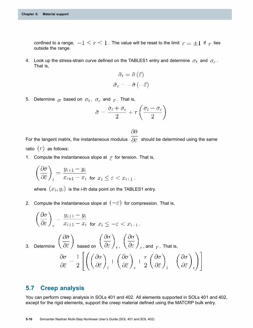
Chapter 5: Material support
confined to a range, . The value will be reset to the limit if liesoutside the range.
4. Look up the stress-strain curve defined on the TABLES1 entry and determine and .That is,
5. Determine based on , and . That is,
For the tangent matrix, the instantaneous modulus should be determined using the same
ratio as follows:
1. Compute the instantaneous slope at for tension. That is,
for .
where is the i-th data point on the TABLES1 entry.
2. Compute the instantaneous slope at for compression. That is,
for .
3. Determine based on , , and . That is,
5.7 Creep analysisYou can perform creep analysis in SOLs 401 and 402. All elements supported in SOLs 401 and 402,except for the rigid elements, support the creep material defined using the MATCRP bulk entry.
5-16 Simcenter Nastran Multi-Step Nonlinear User’s Guide (SOL 401 and SOL 402)
Chapter 5: Material support
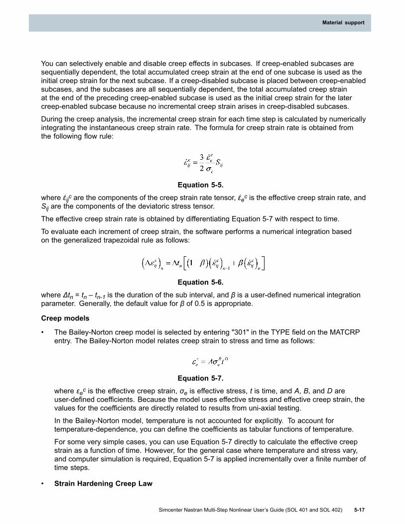
Material support
You can selectively enable and disable creep effects in subcases. If creep-enabled subcases aresequentially dependent, the total accumulated creep strain at the end of one subcase is used as theinitial creep strain for the next subcase. If a creep-disabled subcase is placed between creep-enabledsubcases, and the subcases are all sequentially dependent, the total accumulated creep strainat the end of the preceding creep-enabled subcase is used as the initial creep strain for the latercreep-enabled subcase because no incremental creep strain arises in creep-disabled subcases.
During the creep analysis, the incremental creep strain for each time step is calculated by numericallyintegrating the instantaneous creep strain rate. The formula for creep strain rate is obtained fromthe following flow rule:
Equation 5-5.
where έijc are the components of the creep strain rate tensor, έec is the effective creep strain rate, andSij are the components of the deviatoric stress tensor.
The effective creep strain rate is obtained by differentiating Equation 5-7 with respect to time.
To evaluate each increment of creep strain, the software performs a numerical integration basedon the generalized trapezoidal rule as follows:
Equation 5-6.
where Δtn = tn – tn-1 is the duration of the sub interval, and β is a user-defined numerical integrationparameter. Generally, the default value for β of 0.5 is appropriate.
Creep models
• The Bailey-Norton creep model is selected by entering "301" in the TYPE field on the MATCRPentry. The Bailey-Norton model relates creep strain to stress and time as follows:
Equation 5-7.
where εec is the effective creep strain, σe is effective stress, t is time, and A, B, and D areuser-defined coefficients. Because the model uses effective stress and effective creep strain, thevalues for the coefficients are directly related to results from uni-axial testing.
In the Bailey-Norton model, temperature is not accounted for explicitly. To account fortemperature-dependence, you can define the coefficients as tabular functions of temperature.
For some very simple cases, you can use Equation 5-7 directly to calculate the effective creepstrain as a function of time. However, for the general case where temperature and stress vary,and computer simulation is required, Equation 5-7 is applied incrementally over a finite number oftime steps.
• Strain Hardening Creep Law
Simcenter Nastran Multi-Step Nonlinear User’s Guide (SOL 401 and SOL 402) 5-17
Material support

Chapter 5: Material support
The strain hardening creep law is selected by entering either "1" or "STRNHARD" in the TYPEfield on the MATCRP entry.
The C1, C2, C3, and C4 coefficients are used to define the strain hardening creep modelas follows:
where εcr is the effective creep strain, σ is the effective stress, and T is the temperature.
A fatal error occurs if any of the C1, C2, or C3 fields are left blank. If C4 is left blank, thetemperature term is ignored.
• Norton Creep Law
The Norton creep law is selected by entering either "2" or "NORTON" in the TYPE field on theMATCRP entry.
The C1, C2, and C4 coefficients are used to define the Norton creep model as follows:
A fatal error occurs if either of the C1 or C2 fields are left blank. If C4 is left blank, the temperatureterm is ignored.
• Generalized Garofalo Creep Law
The generalized Garofalo creep law is selected by entering either "3" or "GENGAROF" in theTYPE field on the MATCRP entry.
The C1, C2, C3, and C4 coefficients are used to define the generalized Garofalo creep modelas follows:
A fatal error occurs if any of the C1, C2, or C3 fields are left blank.
If C4 is left blank, the temperature term is ignored.
User interface
• With the MATNL parameter, you can globally switch the creep analysis capability on or off.
For more information, see the MATNL parameter.
• Parameters are available for use with the NLCNTL bulk entry for SOL 401 or the NLCNTL2 bulkentry for SOL 402. These parameters allow you to turn off the creep capability in subcases,control adaptive time stepping or define a constant time step, and define the integration factorin Equation 5-6.
For more information, see the NLCNTL bulk entry for SOL 401 or the NLCNTL2 bulk entry forSOL 402 in the Simcenter Nastran Quick Reference Guide.
• With the MATCRP bulk entry, you define parameters related to the creep constitutive model.
For more information, see the MATCRP bulk entry in the Simcenter Nastran Quick ReferenceGuide.
5-18 Simcenter Nastran Multi-Step Nonlinear User’s Guide (SOL 401 and SOL 402)
Chapter 5: Material support

Material support
• You can use the parameter TABS to convert the temperature units for creep materials. For moreinformation, see Converting temperature units for creep materials.
Activating creep analysis
To activate the creep analysis capability in SOLs 401 or 402, do the following:
1. Reference both the MAT1 and MATCRP bulk entries in the regions where creep occurs.
2. Specify PARAM,MATNL,1.
3. Include a NLCNTL case control command that points to a NLCNTL bulk entry for SOL 401, or aNLCNTL2 bulk entry for SOL 402.
4. On the NLCNTL/NLCNTL2 bulk entry, specify any applicable parameters.
If your input file contains subcases, and you want to include the effects of creep in specific subcases,but not others, you have two options.
Option 1: Use a global NLCNTL case control command
1. Specify PARAM,MATNL,1.
2. Include a NLCNTL case control command above the subcases that points to a NLCNTL/NLCNTL2bulk entry.
3. On the NLCNTL/NLCNTL2 bulk entry, specify applicable parameters.
4. In the subcases in which you want to disable the creep analysis capability, include a NLCNTLcase control command that points to a NLCNTL/NLCNTL2 bulk entry.
5. On the NLCNTL/NLCNTL2 bulk entry, specify the following:
• "CREEP” in a PARAMi field.
• “NO” in the corresponding VALUEi field.
Option 2: Include NLCNTL case control commands in every subcase
1. Specify PARAM,MATNL,1.
2. Include NLCNTL case control commands in each subcase. Multiple NLCNTL case controlcommands can point to a single NLCNTL/NLCNTL2 bulk entry.
3. In subcases in which you want to enable the creep analysis capability, point the NLCNTL casecontrol command to a NLCNTL/NLCNTL2 bulk entry with applicable parameters specified.
4. In subcases in which you want to disable the creep analysis capability, point the NLCNTL casecontrol command point to a NLCNTL/NLCNTL2 bulk entry with the following specified:
• “CREEP” in a PARAMi field.
• “NO” in the corresponding VALUEi field.
Simcenter Nastran Multi-Step Nonlinear User’s Guide (SOL 401 and SOL 402) 5-19
Material support
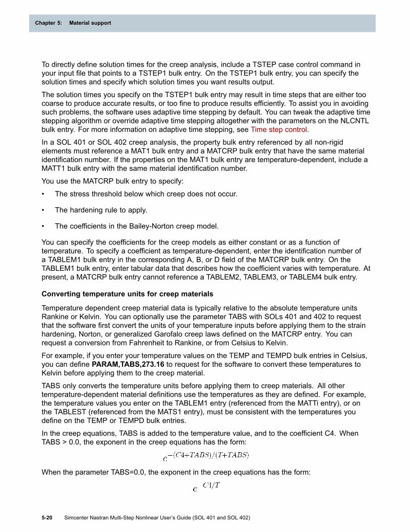
Chapter 5: Material support
To directly define solution times for the creep analysis, include a TSTEP case control command inyour input file that points to a TSTEP1 bulk entry. On the TSTEP1 bulk entry, you can specify thesolution times and specify which solution times you want results output.
The solution times you specify on the TSTEP1 bulk entry may result in time steps that are either toocoarse to produce accurate results, or too fine to produce results efficiently. To assist you in avoidingsuch problems, the software uses adaptive time stepping by default. You can tweak the adaptive timestepping algorithm or override adaptive time stepping altogether with the parameters on the NLCNTLbulk entry. For more information on adaptive time stepping, see Time step control.
In a SOL 401 or SOL 402 creep analysis, the property bulk entry referenced by all non-rigidelements must reference a MAT1 bulk entry and a MATCRP bulk entry that have the same materialidentification number. If the properties on the MAT1 bulk entry are temperature-dependent, include aMATT1 bulk entry with the same material identification number.
You use the MATCRP bulk entry to specify:
• The stress threshold below which creep does not occur.
• The hardening rule to apply.
• The coefficients in the Bailey-Norton creep model.
You can specify the coefficients for the creep models as either constant or as a function oftemperature. To specify a coefficient as temperature-dependent, enter the identification number ofa TABLEM1 bulk entry in the corresponding A, B, or D field of the MATCRP bulk entry. On theTABLEM1 bulk entry, enter tabular data that describes how the coefficient varies with temperature. Atpresent, a MATCRP bulk entry cannot reference a TABLEM2, TABLEM3, or TABLEM4 bulk entry.
Converting temperature units for creep materials
Temperature dependent creep material data is typically relative to the absolute temperature unitsRankine or Kelvin. You can optionally use the parameter TABS with SOLs 401 and 402 to requestthat the software first convert the units of your temperature inputs before applying them to the strainhardening, Norton, or generalized Garofalo creep laws defined on the MATCRP entry. You canrequest a conversion from Fahrenheit to Rankine, or from Celsius to Kelvin.
For example, if you enter your temperature values on the TEMP and TEMPD bulk entries in Celsius,you can define PARAM,TABS,273.16 to request for the software to convert these temperatures toKelvin before applying them to the creep material.
TABS only converts the temperature units before applying them to creep materials. All othertemperature-dependent material definitions use the temperatures as they are defined. For example,the temperature values you enter on the TABLEM1 entry (referenced from the MATTi entry), or onthe TABLEST (referenced from the MATS1 entry), must be consistent with the temperatures youdefine on the TEMP or TEMPD bulk entries.
In the creep equations, TABS is added to the temperature value, and to the coefficient C4. WhenTABS > 0.0, the exponent in the creep equations has the form:
When the parameter TABS=0.0, the exponent in the creep equations has the form:
5-20 Simcenter Nastran Multi-Step Nonlinear User’s Guide (SOL 401 and SOL 402)
Chapter 5: Material support

Material support
You must define C4 if you want a temperature dependent creep material. C4 has no default, and if leftblank, the software will ignore the temperature term in the creep laws.
If TABS is undefined, TABS=0.0 is used.
Time step control
During a SOL 401 or a SOL 402 creep analysis, the solution times depend on:
• How you specify the TSTEP1 bulk entry.
• How you specify the time stepping parameters.
The time steps that result from the TSTEP1 bulk entry specification may be too coarse to produceaccurate results, or too fine to produce results efficiently. By default, the software uses an adaptivetime stepping algorithm to avoid such problems.
Tweaking the adaptive time stepping algorithm in SOL 401
In SOL 401, you can tweak the adaptive time stepping algorithm or override adaptive time steppingaltogether and use a constant time step with parameters for the NLCNTL bulk entry. The parametersare:
CRCERAT Ratio of maximum creep increment to elastic strain that is used to adaptivelyspecify the next time step.
CRCINC Maximum creep increment that is used to adaptively specify the next time step.
CRICOFF Creep strain increment below which the next time step is the product of thecurrent time step and the maximum time step multiplying factor.
CRINFAC Numerical integration parameter.
See Equation 5-6.
DTINIT Initial time step for adaptive time stepping, or the constant time step if adaptivetime stepping is overridden.
CRMFMN Minimum time step multiplying factor.
CRMFMX Maximum time step multiplying factor.
DTSBCDT Controls whether the first time step in a sequential subcase uses the initial timestep or the time step calculated at the end of the previous subcase.
CRTEABS Maximum absolute truncation error that is used to adaptively specify the nexttime step.
CRTECO Effective creep strain below which CRTEABS is used, and above whichCRTEREL is used.
CRTEREL Maximum relative truncation error that is used to adaptively specify the nexttime step.
TSCCR Specifies the time stepping method.
DTMIN Minimum time step.
DTMAX Maximum time step.
Simcenter Nastran Multi-Step Nonlinear User’s Guide (SOL 401 and SOL 402) 5-21
Material support

Chapter 5: Material support
The TSCCR parameter controls the overall time stepping behavior. Use the TSCCR parameter to:
• Select the adaptive time stepping algorithm that the software uses to calculate the next time step.
• Override adaptive time stepping altogether and have the software use the value of the DTINITparameter as a constant time step.
The adaptive time stepping algorithm options include the following:
• The next time step is based on the maximum creep strain increment criterion. You specify themaximum creep strain increment with the CRCINC parameter.
• The next time step is based on the ratio of maximum creep increment to elastic strain criterion.You specify the ratio of maximum creep increment to elastic strain with the CRCERAT parameter.
• The next time step is based on the maximum truncation error criterion. For this option, youhave three sub-options.
o Use the maximum absolute truncation error. You specify the maximum absolute truncationerror with the CRTEABS parameter.
o Use the maximum relative truncation error. You specify the maximum relative truncationerror with the CRTEREL parameter.
o Use the maximum absolute truncation error if the creep strain is less than the value specifiedby the CRTECO parameter, and use the maximum relative truncation error if the creep strainis greater than the value specified by the CRTECO parameter.
• The next time step is the shortest time step calculated by any combination of the maximum creepstrain increment, ratio of maximum creep increment to elastic strain, and maximum truncationerror criteria.
When the creep simulation begins, the value of the DTINIT parameter is always used as the firsttime step. If adaptive time stepping is overridden, the value of the DTINIT parameter is used as aconstant time step throughout the simulation.
If adaptive time stepping is not overridden, after each time step the software compares the calculatedcreep strain increment to the value of the CRICOFF parameter. If the creep strain increment isgreater than the value of the CRICOFF parameter, the software uses the adaptive time steppingalgorithm to calculate the next time step. If the creep strain increment is less than the value ofthe CRICOFF parameter, the software uses the product of the current time step and the value ofthe CRMFMX parameter as the next time step.
If the software uses the adaptive time stepping algorithm to calculate the next time step, the next timestep is compared to the product of the current time step and the value for the CRMFMN parameter. Ifthe next time step is smaller than the product of the current time step and the value for the CRMFMNparameter, the software halves the current time step, recalculates the current creep strain increment,and reenters the algorithm at the point the creep strain increment is compared to the value of theCRICOFF parameter. If the next time step is larger than the product of the current time step and thevalue of the CRMFMN parameter, the software keeps the next time step.
The next time step is then compared against the values of the DTMAX and DTMIN parameters. First,the software checks to see if the value of the DTMAX parameter is 0.0. If so, the software accepts thevalue for the next time step and uses it to compute the next creep strain increment. If the value of
5-22 Simcenter Nastran Multi-Step Nonlinear User’s Guide (SOL 401 and SOL 402)
Chapter 5: Material support

Material support
the DTMAX parameter is not set to 0.0, the next time step is compared to the value of the DTMAXparameter. If the next time step is larger than the value of the DTMAX parameter, the software usesthe value of the DTMAX parameter as the next time step and uses it to compute the next creepstrain increment. If the next time step is smaller than the value of the DTMAX parameter, the nexttime step is compared to the value of the DTMIN parameter. If the next time step is smaller thanthe value for the DTMIN parameter, the software halves the current time step, recalculates thecurrent creep strain increment, and reenters the algorithm at the point the creep strain increment iscompared to the CRICOFF parameter. If the next time step is larger than the value of the DTMINparameter, the software accepts the value for the next time step and uses it to compute the nextcreep strain increment.
The adaptive time stepping algorithm is summarized by the following flowchart. In the flowchart, thenotation for the value of a parameter is Vparameter name.
Simcenter Nastran Multi-Step Nonlinear User’s Guide (SOL 401 and SOL 402) 5-23
Material support

Chapter 5: Material support
Figure 5-2. Flowchart of adaptive time stepping algorithm
Regardless of whether you are using adaptive time stepping or a constant time step, the solutiontimes you specify with the TENDi and NINCi fields on TSTEP1 bulk entries are always honored. At alltimes during the creep simulation, if the next time step would result in skipping over a TSTEP1-definedsolution time, the software truncates the next time step so that a solve occurs at that solution time.
As a best practice, consider using the TSTEP1 bulk entry to specify only the times you want theresults output, and let the adaptive time stepping algorithm determine all the other solution times.
For additional information on the creep-related parameters, see the NLCNTL bulk entry in theSimcenter Nastran Quick Reference Guide.
5-24 Simcenter Nastran Multi-Step Nonlinear User’s Guide (SOL 401 and SOL 402)
Chapter 5: Material support
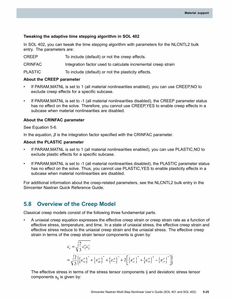
Material support
Tweaking the adaptive time stepping algorithm in SOL 402
In SOL 402, you can tweak the time stepping algorithm with parameters for the NLCNTL2 bulkentry. The parameters are:
CREEP To include (default) or not the creep effects.
CRINFAC Integration factor used to calculate incremental creep strain
PLASTIC To include (default) or not the plasticity effects.
About the CREEP parameter
• If PARAM,MATNL is set to 1 (all material nonlinearities enabled), you can use CREEP,NO toexclude creep effects for a specific subcase.
• If PARAM,MATNL is set to -1 (all material nonlinearities disabled), the CREEP parameter statushas no effect on the solve. Therefore, you cannot use CREEP,YES to enable creep effects in asubcase when material nonlinearities are disabled.
About the CRINFAC parameter
See Equation 5-6.
In the equation, β is the integration factor specified with the CRINFAC parameter.
About the PLASTIC parameter
• If PARAM,MATNL is set to 1 (all material nonlinearities enabled), you can use PLASTIC,NO toexclude plastic effects for a specific subcase.
• If PARAM,MATNL is set to -1 (all material nonlinearities disabled), the PLASTIC parameter statushas no effect on the solve. Thus, you cannot use PLASTIC,YES to enable plasticity effects in asubcase when material nonlinearities are disabled.
For additional information about the creep-related parameters, see the NLCNTL2 bulk entry in theSimcenter Nastran Quick Reference Guide.
5.8 Overview of the Creep ModelClassical creep models consist of the following three fundamental parts.
• A uniaxial creep equation expresses the effective creep strain or creep strain rate as a function ofeffective stress, temperature, and time. In a state of uniaxial stress, the effective creep strain andeffective stress reduce to the uniaxial creep strain and the uniaxial stress. The effective creepstrain in terms of the creep strain tensor components is given by:
The effective stress in terms of the stress tensor components ij and deviatoric stress tensorcomponents sij is given by:
Simcenter Nastran Multi-Step Nonlinear User’s Guide (SOL 401 and SOL 402) 5-25
Material support

Chapter 5: Material support
• A flow rule determines the creep strain rate tensor components for a general state of stress.
• A hardening rule determines creep strain rates from the uniaxial rate equation under changingstress and temperature.
Overview of the Hardening Rules for Creep Models
The hardening rule provides the mathematical means to determine the effective creep rate underchanging temperature and/or stress. The creep hardening rule is used to determine the currentmaterial state relative to further creep straining. It plays a role similar to the yield surface in plasticitytheory.
You can select one of the following hardening rules for the creep model using the HARD field on theMATCRP bulk entry.
• HARD = STRAIN (default) selects strain hardening.
• HARD = TIME selects time hardening.
Strain Hardening
The strain hardening rule assumes that the material state is determined by the accumulated effectivecreep strain. When stress or temperature changes, the shift from one creep curve to another is basedon the accumulated effective creep strain. This shift is illustrated in the following figure.
5-26 Simcenter Nastran Multi-Step Nonlinear User’s Guide (SOL 401 and SOL 402)
Chapter 5: Material support
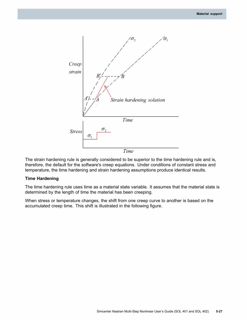
Material support
The strain hardening rule is generally considered to be superior to the time hardening rule and is,therefore, the default for the software's creep equations. Under conditions of constant stress andtemperature, the time hardening and strain hardening assumptions produce identical results.
Time Hardening
The time hardening rule uses time as a material state variable. It assumes that the material state isdetermined by the length of time the material has been creeping.
When stress or temperature changes, the shift from one creep curve to another is based on theaccumulated creep time. This shift is illustrated in the following figure.
Simcenter Nastran Multi-Step Nonlinear User’s Guide (SOL 401 and SOL 402) 5-27
Material support

Chapter 5: Material support
The time hardening rule is usually not very realistic when very large changes in temperature orstress occur over the interval of interest.
Maximum Truncation Error Criterion
With the maximum truncation error criterion, Simcenter Nastran also calculates the next time stepby scaling the current time step. The value of the CRTECO parameter on the NLCNTL bulk entrydetermines whether the maximum absolute truncation error or the maximum relative truncation erroris used to adaptively specify the next time step.
• If the effective creep strain is less than the value of the CRTECO parameter, the maximumabsolute truncation error is used. The maximum absolute truncation error is specified with theCRTEABS parameter on the NLCNTL bulk entry.
• If the effective creep strain is greater than the value of the CRTECO parameter, the maximumrelative truncation error is used. The maximum relative truncation error is specified with theCRTEREL parameter on the NLCNTL bulk entry.
The next time step is calculated by scaling the current time. When the maximum absolute truncationerror is applied, the software computes the next time step as:
When the maximum relative truncation error is applied, the software computes the next time step as:
5-28 Simcenter Nastran Multi-Step Nonlinear User’s Guide (SOL 401 and SOL 402)
Chapter 5: Material support

Material support
where e is the calculated truncation error, and is the current effective creep strain increment.There are two approaches to calculate the truncation error e corresponding to the two differentscenarios:
1. At the first time step or if β=0 or β=1, the two point rule truncation error is used.
2. From the second time step and 0 < β< 1, the three point rule truncation error is used.
Maximum creep strain increment criterion
With the maximum creep strain increment criterion, Simcenter Nastran calculates the next timestep by scaling the current time step as follows:
Equation 5-8.
where CRCINC is the value of the CRCINC parameter and Δεec is the current effective creep strainincrement.
Ratio of maximum creep increment to elastic strain criterion
With the ratio of maximum creep increment to elastic strain criterion, Simcenter Nastran calculatesthe next time step by scaling the current time as follows:
Equation 5-9.
where CRCERAT is the value of the CRCERAT parameter, Δεec is the current effective creep strainincrement, and εeE is the current total effective elastic strain.
5.9 User defined materialsSOLs 401 and 402 support externally computed, user defined material models. You can define amaterial model by developing and compiling an external routine. The external routine can optionallyinclude multiple material models.
Source code examples are included with the Simcenter Nastran installation for you to begin yourown external material development. A Ready-to-run routine and test cases are also included todemonstrate the input file requirements and the general workflow.
Simcenter Nastran Multi-Step Nonlinear User’s Guide (SOL 401 and SOL 402) 5-29
Material support

Chapter 5: Material support
You can develop an external material routine using FORTRAN or C, and compile for Windows orLinux operating systems.
Simcenter Nastran Inputs
The MUMAT bulk entry is available to define the material data in the Simcenter Nastran input file.Simcenter Nastran passes this data to the external routine. The MUMAT entry in your input file isthe trigger Simcenter Nastran uses to call the external routine.
The elements referencing the MUMAT entry material ID will use an associated material lawdefined in the user defined material routine NXUMAT. See NXUMAT interface for the NXUMATAPI description. The elements referencing the MUMAT entry must also reference MAT1, MAT2,MAT8, MAT9, MAT11, and MATCZ entries. Simcenter Nastran uses the MATi properties to computethe initial elastic stiffness. Temperature dependent materials are also supported and are used bySimcenter Nastran when computing the initial elastic stiffness. The initial elastic stiffness computedby Simcenter Nastran and the data defined on the MATi, MATTI, and TABLEMi entries are all passedfrom Simcenter Nastran to the external routine.
All of the data defined on the MUMAT bulk entry is also passed to the NXUMAT routine. You caninclude a variety data types on the MUMAT entry. For example, real, integer, tables and table oftables can all be included.
The following data is supported on the MUMAT entry:
• MODNAME1 and MODNAME2 fields - Optional character fields.
• MATNAME field - Can be used to request a specific material model.
• NUMSTAT field - Defines the total number of state variables, if they exist.
The following tabular data is supported on the MUMAT entry:
Note: When you reference TABLES1, TABLEM1, TABLEST entries on the MUMAT entry, SimcenterNastran does no interpolation or extrapolation of the data before passing it to the external routine.
• TABLES1 - This is a collection of real data pairs. You reference the ID of TABLES1 entriesdefined in your Simcenter Nastran input file.
• TABLEM1 - This is a collection of real data pairs. You reference the ID of TABLEM1 entriesdefined in your Simcenter Nastran input file.
• TABLEST - This is a collection real data values versus table ID’s. The table ID's reference othertables with a collection of real data pairs. You reference the ID of TABLEST entries defined inyour Simcenter Nastran input file.
Simcenter Nastran also optionally stores, retrieves, and outputs state variable data computed bythe external routine. For example, stress, creep strain and plastic strain at each solution incrementcan be stored as state variables. You define the number of state variables in the NUMSTAT field onthe MUMAT entry, and Simcenter Nastran will initialize the appropriate storage. The flow of statevariable data is as follows:
• Your external routine provides Simcenter Nastran with updated state variables at the end of atime step.
• Simcenter Nastran stores the variables in the database.
5-30 Simcenter Nastran Multi-Step Nonlinear User’s Guide (SOL 401 and SOL 402)
Chapter 5: Material support

Material support
• Simcenter Nastran provides the data back to the external routine at the beginning of theconsecutive time step.
You can request Simcenter Nastran to output the state variables using the STATVAR case controlcommand. Regardless of what the data is originally, for example, vector or tensor components,Simcenter Nastran outputs all of the state variable data as scalar values. The GRID/GAUSS outputoption is also available on the STATVAR command.
You can pass parameters defined in the Simcenter Nastran input file to the external routine. Thisincludes parameters defined with the PARAM case control, the PARAM bulk entry, and the PLASTIC,CREEP, and the MATNL parameter settings defined on the NLCNTL (SOL 401) or NLCNTL2 (SOL402) bulk entry. You can use these settings in your external routine, for example, to turn on/offspecific material computations in a subcase.
NXUMAT interface
The subroutine NXUMAT directs Simcenter Nastran to a specific material model. A shared library(DLL/SO file) is built from this routine and used by Simcenter Nastran to model the material behavior.The building process of the shared library is described in Compiling instructions.
The arguments of NXUMAT are detailed below. Simcenter Nastran expects that the real, integerand character values passed from the argument list are of precision REAL*8, INTEGER*8 andCHARACTER (LEN=8).
SUBROUTINE NXUMAT(IOPER, MODNAME1, MODNAME2, MATID, HOOK, TANSTIFF,MATIR, MATIN, NMATI, MUDATAR, MUDATAI, NMUDATA ,DFGRDT0, DFGRDT1, EPSTOTT1, EPSMT1, EPSTHT1, EPSDELM,DELTAT, TIMET1, TEMPT0, TEMPT1, NB, INTVALS,REALVALS, XYZT1, ROT, NXPARAM, STATEVAR, NSVAR,SIGMA, EPSPL, EPSCR, DTRATIO, VOID1, VOID2, VOID3, IRET)
FUNCTION : USER MATERIAL DEFINITIONTHIS ROUTINE IS DIVIDED IN THREE STEPS (IOPER)
IF (IOPER.EQ.0) THENNXUMAT DLL VERSION NUMBER
ELSEIF (IOPER.EQ.1) THENINITIALIZATION OF STATEVAR
ELSECOMPUTATION OF MATERIAL LAW
ENDIFEND
Each of the arguments of the NXUMAT routine is described below.
IOPER (Input)
IOPER defines the operational step for which NXUMAT has been called for.
IOPER = 0: this is used to facilitate versioning for the NXUMAT library. This number is read fromthe argument STATEVAR(1). This float is printed to the F06 file as a user information message23209 along with the value In STATEVAR(1).
Example
*** USER INFORMATION MESSAGE 23209 (IFPDRV)
Simcenter Nastran Multi-Step Nonlinear User’s Guide (SOL 401 and SOL 402) 5-31
Material support

Chapter 5: Material support
VERSION 1.00 OF NXUMAT DLL LOADED.
IOPER=1: This is used to initialize state variables. This step can be used to assign initial values tothe STAEVAR array, which will be stored by Simcenter Nastran and returned in the computationalstep.
IOPER=2: This is considered the computational step.
IOPER=3: This is used to return Hooke’s matrix.
Note
IOPER = 3 is not used in SOL 402.
MODNAME1 (Input)
MODNAME1 contains the eight-character name from the MUMAT entry.
MODNAME2 (Input)
MODNAME2 contains the eight-character name from the MUMAT entry.
MATID (Input)
MATID is the material ID given in the MUMAT entry.
HOOK(NB,NB) (Input)
HOOK is an NBxNB-size matrix containing Hooke’s matrix. This is pre-computed by SimcenterNastran based on the MATi entries associated with the MUMAT entry.
TANSTIFF(NB,NB) (Input/Output)
TANSTIFF contains the tangent stiffness matrix computed at the previous time step when enteringNXUMAT and should be updated with the tangent stiffness matrix for the current time stepupon convergence.
MATIR(NMATI) (Input)
MATIR contains the real data from the associated MATi entries. Its format is explained inMATIN/MATIR array format.
MATIN(NMATI) (Input)
MATIN contains the integer data from the associated MATi entries. Its format is explained inMATIN/MATIR array format.
NMATI (Input)
NMATI is the size of the MATIR/MATIN array.
MUDATAR (NMUDATA) (Input)
MUDATAR contains the real data from the MUMAT entries. Its format is explained inMUDATAI/MUDATAR array format.
5-32 Simcenter Nastran Multi-Step Nonlinear User’s Guide (SOL 401 and SOL 402)
Chapter 5: Material support

Material support
MUDATAI (NMUDATA) (Input)
MUDATAI contains the integer data from the MUMAT entry. Its format is explained inMUDATAI/MUDATAR array format.
NMUDATA (Input)
NMUDATA is the size of the MUDATAR/MUDATAI array.
DFGRDT0(3,3) (Input)
Deformation gradient at the previous time step. This is currently undefined.
DFGRDT1(3,3) (Input)
Deformation gradient at the previous time step. This is currently undefined.
EPSTOTT1(NB) (Input)
Total strain tensor (including mechanical and thermal strain).
EPSMT1(NB) (Input)
Mechanical strain.
EPSTHT1(NB) (Input)
Thermal strain.
EPSDELM(NB) (Input)
Mechanical strain increment.
DELTAT (Input)
Time step.
TIMET1 (Input)
Current time.
TEMPT0 (Input)
Temperature at the previous time step.
TEMPT1 (Input)
Temperature at the current time step.
NB (Input)
Number of tensor components.
Note
For SOL 402, NB=6 contains all element types, including axisymmetric, plane strain,and shell elements.
Simcenter Nastran Multi-Step Nonlinear User’s Guide (SOL 401 and SOL 402) 5-33
Material support

Chapter 5: Material support
INTVALS(*) (Input)
The INTVALS array contains various integer data, including the following:
INTVALS(1) contains the element ID.
INTVALS(2) contains the Gauss ID.
INTVALS(3) contains the current time step number.
INTVALS(4) contains the iteration number for the current time step.
INTVALS(5) contains the subcase ID.
INTVALS(6) contains the material type such as plane strain.
INTVALS(7) contains a standard tangential matrix at the point of convergence, which is usedat the beginning of the next step for plasticity models. (SOL 401)
Note
For SOL 402, the INTVAL(7) convergence flag does not apply because the UMATroutine is not called after convergence.
REALVALS(*) (Input)
The REALVALS array contains various real data, including the following:
REALVALS(1) contains the element thickness for shell elements.
XYZT1(3) (Input)
XYZT1 contains the updated coordinates of the current Gauss point.
Note
Not available for SOL 402. For SOL 402, the initial Gauss point coordinates for solid,plane strain, and axisymmetric elements are provided.
ROT(3,3) (Input)
ROT contains the rotational matrix between the structural and material coordinate systems.
Note
Not available for SOL 401. For SOL 402, the initial rotational matrix for only solid,plane strain, and axisymmetric elements is provided.
NXPARAM(*) (Input)
NXPARAM contains the list of PARAM entry values that are in the input test case. You can passparameters defined in the Simcenter Nastran input file to the external routine. This includes
5-34 Simcenter Nastran Multi-Step Nonlinear User’s Guide (SOL 401 and SOL 402)
Chapter 5: Material support

Material support
parameters defined with the PARAM case control, the PARAM bulk entry, and the PLASTIC,CREEP, and MATNL parameter settings defined on the NLCNTL (SOL 401) or NLCNTL2 (SOL402) bulk entry. You can use these settings in your external routine, for example, to turn on/offspecific material computations in a subcase. Refer to the included utility routine PARAMQRYto understand how to use this functionality.
Note
For SOL 402, this is restricted to LGDISP, LGSTRN, K6ROT, SNORM, W3/4,ALPHA1/2, G, MATNL, NLAYERS, NOFISR, SRCOMPS, MAXRATIO, and AFNORM.
STATEVAR(NSVAR) (Input/Output)
STATEVAR contains the state variables that you specified. It contains the previous time stepstate variables as input and must be updated with current state variables upon convergence.
NSVAR (Input)
NSVAR is the number of state variables.
Note
The UMAT developer must perform error checking with this argument if the valuespecified on the MUMAT card is not consistent with the expected state variable vectorlength.
SIGMA(NB) (Input/Output)
SIGMA contains the stress tensor from the previous time step and must be updated with thecurrent time step value upon convergence.
EPSPL(NB) (Input/Output)
EPSPL contains the plastic strain tensor from the previous time step and must be updatedwith current time step value upon convergence. This strain tensor is stored inside SimcenterNastran and is output when requested.
EPSCR(NB) (Input/Output)
EPSCR contains the creep strain tensor from the previous time step and must be updated withcurrent time step value upon convergence. This strain tensor is stored inside Simcenter Nastranand is output when requested.
DTRATIO (Output)
DTRATIO is the next time step to the current time step ratio. It can be specified by the user frominside NXUMAT to control the time stepping scheme. If the output of this variable is 0, it is ignored.When DTRATIO < 0 we terminate the time step and start a new one with reduced time step.
Simcenter Nastran Multi-Step Nonlinear User’s Guide (SOL 401 and SOL 402) 5-35
Material support

Chapter 5: Material support
Note
For SOLs 401 and 402, if the material has no viscous effect, the output is 0, andthis is ignored.
VOID1, VOID2, VOID3
These are empty slots for future use.
IRET (Output)
IRET is the return code. Any returned value other than 0 (>0) will stop the solution and issue afatal message with the return code.
The user data specified on the MUMAT entry and corresponding MATi entry is passed to the NXUMATroutine via the arrays MUDATAI/MUDATAR and MATIN/MATIR respectively. This section describesthe layout of the input data arrays supplied to the NXUMAT subroutine.
Each entry (that is, the MUMAT entry and the MATi* entry) is stored in two arrays each. One arrayhas the integer data and the other has the real data. Some cross-referencing between the two arraysmust be done to extract the desired data. The format of these arrays is described in the followingsections. These arrays are declared as INTEGER*8 for the integers and REAL*8 for the real portion.
MATIN/MATIR array format
MATi data along with corresponding MATTi entries are sent to the NXUMAT routine through twoarrays: MATIN and MATIR. Both MATIN and MATIR represent the MATi entry data in the format laidout in the following table. The integer data of the MATi and MATTi entries exist in MATIN and thereal data exist in the MATIR array.
The first word in the array is the total number of words in the array. The second word is the offset tothe mapping array. The mapping array has information on the location of each table of data. The thirdword identifies the type of the array: 1 corresponds to the MATIN array and 2 corresponds to theMUDATAI array. The fourth word is the material ID, and the fifth word contains the type of the MATientry. Based on the type of MATi entry for which this array contains data, the next ‘N’ words fromthe sixth word contain the bulk entry data (N=11, 20, and 15 for the MATi entry respectively). Afterthat, in the next word (if any), corresponding MATTi entries are present, including its ID. If no MATTientries are present, this word is zero. If the MATTi entry is present, after the ID the MATTi entries arelaid out next. If MATTi entries are present, that means TABLEM1 data is present. This is laid outnext in the array. Each table has a fixed format as shown in the following table and is ended by a -1.Multiple tables can exist. The mapping array is laid out in the end.
Word Description1 Total length of data used in this array (LENGTH).2 Offset to the mapping array (array index).3 The ID code for a MATIN array is always 1.
The ID code is used by the interpolation routines to identify the data structure.4 Material ID used to setup the array.
5-36 Simcenter Nastran Multi-Step Nonlinear User’s Guide (SOL 401 and SOL 402)
Chapter 5: Material support

Material support
Word Description5 MAT table type:
1: The record contains MAT1 data.
9: The record contains MAT9 data.
11: The record contains MAT11 data.6 Number of entries in the record (N):
If the MAT table type is 1, N = 11.
If the MAT table type is 9, N = 20.
If the MAT table type is 11, N = 15.7 through N+6 MAT* constants (real).N+8 MATT* ID (0 if no MATT* entry).N+9 through 2N+8 MATT* entries (integers).N+6 throughLENGTH
TABLEM1 data tables (CODEX/CODEY: 0=Linear, 1=Log):
1. Table identification number (if 0, no table).
2. NUMPAIR: Number of X-Y Pairs.
3. CODEX: Type of interpolation for the x-axis (integer).
4. CODEY: Type of interpolation for the y-axis (integer).
5. EXTRAP: Extrapolation option.
6. X tabular value (real).
7. Y tabular value (real).
- Words 6 through 7 repeated NUMPAIR.
(-1) end of TABLEM1 tables.Mapping
1. Table ID.
2. Array index pointing to the table data.
For example, consider a MAT9 entry as show below along with a MATT9 entry and correspondingTABLEM1 entries.
MAT9 1 1.+7 2.5+6 1.+6 0. 0. 0. 1.+7++ 1.+6 0. 0. 0. 3.+7 0. 0. 0.++ 3.75+6 0. 0. 1.75+6 0. 1.75+6 0.1 1.-5++ 1.-5 1.-5 1.-5 1.-5 1.-5 0.
MATT9 1 1 1+
Simcenter Nastran Multi-Step Nonlinear User’s Guide (SOL 401 and SOL 402) 5-37
Material support
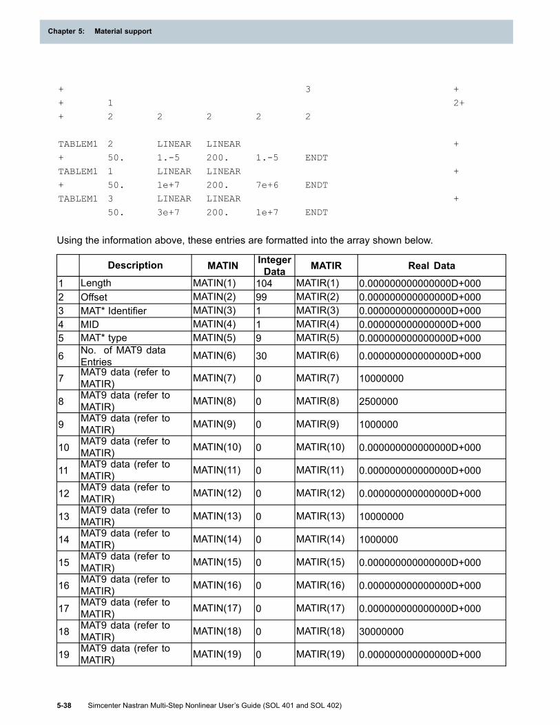
Chapter 5: Material support
+ 3 +
+ 1 2++ 2 2 2 2 2
TABLEM1 2 LINEAR LINEAR +
+ 50. 1.-5 200. 1.-5 ENDT
TABLEM1 1 LINEAR LINEAR +
+ 50. 1e+7 200. 7e+6 ENDT
TABLEM1 3 LINEAR LINEAR +
50. 3e+7 200. 1e+7 ENDT
Using the information above, these entries are formatted into the array shown below.
Description MATIN IntegerData MATIR Real Data
1 Length MATIN(1) 104 MATIR(1) 0.000000000000000D+0002 Offset MATIN(2) 99 MATIR(2) 0.000000000000000D+0003 MAT* Identifier MATIN(3) 1 MATIR(3) 0.000000000000000D+0004 MID MATIN(4) 1 MATIR(4) 0.000000000000000D+0005 MAT* type MATIN(5) 9 MATIR(5) 0.000000000000000D+000
6 No. of MAT9 dataEntries MATIN(6) 30 MATIR(6) 0.000000000000000D+000
7 MAT9 data (refer toMATIR) MATIN(7) 0 MATIR(7) 10000000
8 MAT9 data (refer toMATIR) MATIN(8) 0 MATIR(8) 2500000
9 MAT9 data (refer toMATIR) MATIN(9) 0 MATIR(9) 1000000
10 MAT9 data (refer toMATIR) MATIN(10) 0 MATIR(10) 0.000000000000000D+000
11 MAT9 data (refer toMATIR) MATIN(11) 0 MATIR(11) 0.000000000000000D+000
12 MAT9 data (refer toMATIR) MATIN(12) 0 MATIR(12) 0.000000000000000D+000
13 MAT9 data (refer toMATIR) MATIN(13) 0 MATIR(13) 10000000
14 MAT9 data (refer toMATIR) MATIN(14) 0 MATIR(14) 1000000
15 MAT9 data (refer toMATIR) MATIN(15) 0 MATIR(15) 0.000000000000000D+000
16 MAT9 data (refer toMATIR) MATIN(16) 0 MATIR(16) 0.000000000000000D+000
17 MAT9 data (refer toMATIR) MATIN(17) 0 MATIR(17) 0.000000000000000D+000
18 MAT9 data (refer toMATIR) MATIN(18) 0 MATIR(18) 30000000
19 MAT9 data (refer toMATIR) MATIN(19) 0 MATIR(19) 0.000000000000000D+000
5-38 Simcenter Nastran Multi-Step Nonlinear User’s Guide (SOL 401 and SOL 402)
Chapter 5: Material support
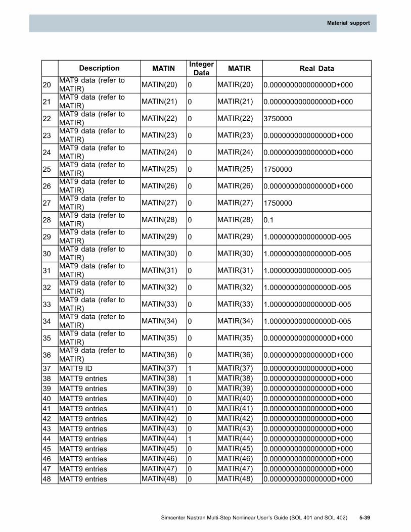
Material support
Description MATIN IntegerData MATIR Real Data
20 MAT9 data (refer toMATIR) MATIN(20) 0 MATIR(20) 0.000000000000000D+000
21 MAT9 data (refer toMATIR) MATIN(21) 0 MATIR(21) 0.000000000000000D+000
22 MAT9 data (refer toMATIR) MATIN(22) 0 MATIR(22) 3750000
23 MAT9 data (refer toMATIR) MATIN(23) 0 MATIR(23) 0.000000000000000D+000
24 MAT9 data (refer toMATIR) MATIN(24) 0 MATIR(24) 0.000000000000000D+000
25 MAT9 data (refer toMATIR) MATIN(25) 0 MATIR(25) 1750000
26 MAT9 data (refer toMATIR) MATIN(26) 0 MATIR(26) 0.000000000000000D+000
27 MAT9 data (refer toMATIR) MATIN(27) 0 MATIR(27) 1750000
28 MAT9 data (refer toMATIR) MATIN(28) 0 MATIR(28) 0.1
29 MAT9 data (refer toMATIR) MATIN(29) 0 MATIR(29) 1.000000000000000D-005
30 MAT9 data (refer toMATIR) MATIN(30) 0 MATIR(30) 1.000000000000000D-005
31 MAT9 data (refer toMATIR) MATIN(31) 0 MATIR(31) 1.000000000000000D-005
32 MAT9 data (refer toMATIR) MATIN(32) 0 MATIR(32) 1.000000000000000D-005
33 MAT9 data (refer toMATIR) MATIN(33) 0 MATIR(33) 1.000000000000000D-005
34 MAT9 data (refer toMATIR) MATIN(34) 0 MATIR(34) 1.000000000000000D-005
35 MAT9 data (refer toMATIR) MATIN(35) 0 MATIR(35) 0.000000000000000D+000
36 MAT9 data (refer toMATIR) MATIN(36) 0 MATIR(36) 0.000000000000000D+000
37 MATT9 ID MATIN(37) 1 MATIR(37) 0.000000000000000D+00038 MATT9 entries MATIN(38) 1 MATIR(38) 0.000000000000000D+00039 MATT9 entries MATIN(39) 0 MATIR(39) 0.000000000000000D+00040 MATT9 entries MATIN(40) 0 MATIR(40) 0.000000000000000D+00041 MATT9 entries MATIN(41) 0 MATIR(41) 0.000000000000000D+00042 MATT9 entries MATIN(42) 0 MATIR(42) 0.000000000000000D+00043 MATT9 entries MATIN(43) 0 MATIR(43) 0.000000000000000D+00044 MATT9 entries MATIN(44) 1 MATIR(44) 0.000000000000000D+00045 MATT9 entries MATIN(45) 0 MATIR(45) 0.000000000000000D+00046 MATT9 entries MATIN(46) 0 MATIR(46) 0.000000000000000D+00047 MATT9 entries MATIN(47) 0 MATIR(47) 0.000000000000000D+00048 MATT9 entries MATIN(48) 0 MATIR(48) 0.000000000000000D+000
Simcenter Nastran Multi-Step Nonlinear User’s Guide (SOL 401 and SOL 402) 5-39
Material support
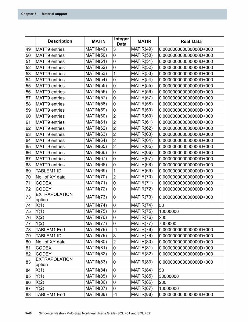
Chapter 5: Material support
Description MATIN IntegerData MATIR Real Data
49 MATT9 entries MATIN(49) 3 MATIR(49) 0.000000000000000D+00050 MATT9 entries MATIN(50) 0 MATIR(50) 0.000000000000000D+00051 MATT9 entries MATIN(51) 0 MATIR(51) 0.000000000000000D+00052 MATT9 entries MATIN(52) 0 MATIR(52) 0.000000000000000D+00053 MATT9 entries MATIN(53) 1 MATIR(53) 0.000000000000000D+00054 MATT9 entries MATIN(54) 0 MATIR(54) 0.000000000000000D+00055 MATT9 entries MATIN(55) 0 MATIR(55) 0.000000000000000D+00056 MATT9 entries MATIN(56) 0 MATIR(56) 0.000000000000000D+00057 MATT9 entries MATIN(57) 0 MATIR(57) 0.000000000000000D+00058 MATT9 entries MATIN(58) 0 MATIR(58) 0.000000000000000D+00059 MATT9 entries MATIN(59) 0 MATIR(59) 0.000000000000000D+00060 MATT9 entries MATIN(60) 2 MATIR(60) 0.000000000000000D+00061 MATT9 entries MATIN(61) 2 MATIR(61) 0.000000000000000D+00062 MATT9 entries MATIN(62) 2 MATIR(62) 0.000000000000000D+00063 MATT9 entries MATIN(63) 2 MATIR(63) 0.000000000000000D+00064 MATT9 entries MATIN(64) 2 MATIR(64) 0.000000000000000D+00065 MATT9 entries MATIN(65) 2 MATIR(65) 0.000000000000000D+00066 MATT9 entries MATIN(66) 0 MATIR(66) 0.000000000000000D+00067 MATT9 entries MATIN(67) 0 MATIR(67) 0.000000000000000D+00068 MATT9 entries MATIN(68) 0 MATIR(68) 0.000000000000000D+00069 TABLEM1 ID MATIN(69) 1 MATIR(69) 0.000000000000000D+00070 No. of XY data MATIN(70) 2 MATIR(70) 0.000000000000000D+00071 CODEX MATIN(71) 0 MATIR(71) 0.000000000000000D+00072 CODEY MATIN(72) 0 MATIR(72) 0.000000000000000D+000
73 EXTRAPOLATIONoption MATIN(73) 0 MATIR(73) 0.000000000000000D+000
74 X(1) MATIN(74) 0 MATIR(74) 5075 Y(1) MATIN(75) 0 MATIR(75) 1000000076 X(2) MATIN(76) 0 MATIR(76) 20077 Y(2) MATIN(77) 0 MATIR(77) 700000078 TABLEM1 End MATIN(78) -1 MATIR(78) 0.000000000000000D+00079 TABLEM1 ID MATIN(79) 3 MATIR(79) 0.000000000000000D+00080 No. of XY data MATIN(80) 2 MATIR(80) 0.000000000000000D+00081 CODEX MATIN(81) 0 MATIR(81) 0.000000000000000D+00082 CODEY MATIN(82) 0 MATIR(82) 0.000000000000000D+000
83 EXTRAPOLATIONoption MATIN(83) 0 MATIR(83) 0.000000000000000D+000
84 X(1) MATIN(84) 0 MATIR(84) 5085 Y(1) MATIN(85) 0 MATIR(85) 3000000086 X(2) MATIN(86) 0 MATIR(86) 20087 Y(2) MATIN(87) 0 MATIR(87) 1000000088 TABLEM1 End MATIN(88) -1 MATIR(88) 0.000000000000000D+000
5-40 Simcenter Nastran Multi-Step Nonlinear User’s Guide (SOL 401 and SOL 402)
Chapter 5: Material support

Material support
Description MATIN IntegerData MATIR Real Data
89 TABLEM1 ID MATIN(89) 2 MATIR(89) 0.000000000000000D+00090 No. of XY data MATIN(90) 2 MATIR(90) 0.000000000000000D+00091 CODEX MATIN(91) 0 MATIR(91) 0.000000000000000D+00092 CODEY MATIN(92) 0 MATIR(92) 0.000000000000000D+000
93 EXTRAPOLATIONoption MATIN(93) 0 MATIR(93) 0.000000000000000D+000
94 X(1) MATIN(94) 0 MATIR(94) 5095 Y(1) MATIN(95) 0 MATIR(95) 1.000000000000000D-00596 X(2) MATIN(96) 0 MATIR(96) 20097 Y(2) MATIN(97) 0 MATIR(97) 1.000000000000000D-00598 TABLEM1 End MATIN(98) -1 MATIR(98) 0.000000000000000D+00099 Mapping array starts.
Table ID, offset givenbelow
MATIN(99) 1 MATIR(99) 0.000000000000000D+000
100 Index to Table ID above MATIN(100) 69 MATIR(100) 0.000000000000000D+000101 Table ID MATIN(101) 3 MATIR(101) 0.000000000000000D+000102 Index to Table ID above MATIN(102) 79 MATIR(102) 0.000000000000000D+000103 Table ID MATIN(103) 2 MATIR(103) 0.000000000000000D+000104 Index to Table ID above MATIN(104) 89 MATIR(104) 0.000000000000000D+000
MUDATAI/MUDATAR array format
The data defined on the MUMAT bulk entry is passed to the NXUMAT routine via the MUDATAI andMUDATAR arrays. Both MUDATAI and MUDATAR represent the MUMAT entry data in the format laidout in the following table. The integer data of MUMAT exist in MUDATAI and the real data exist inthe MUDATAR array.
The first word in the array is the total number words in the array. The second word is the offset tothe mapping array. The mapping array has information of the location of each table of data. Thethird word identifies the type of array: 1 corresponds to the MATIN array and 2 corresponds to theMUDATAI array. The next six words are the data present on the first line of the MUMAT entry. Afterthis, the next word contains a code that identifies the type of data that is to follow (1 for real, 2 forinteger, 3 for TABLES1, 4 for TABLEST, 5 for TABLEM1, and 6 for a mapping array). After the code,the next word is the size of the array for this ‘code data’ followed by the data. Note that multiple typesof data can exist, so expect multiple codes followed by their corresponding data.
After this, the table data is laid out for each TABLES1, TABLEST, and TABLEM1 on the MUMATentry. The format is shown in the following table.
Word Description1 Total length of data used in this array (LENGTH).2 Offset to the mapping array (array index).3 The ID code for a MUDATAI array is 2 for MUMAT.
The ID code is used by the interpolation routines to identify the data structure.4-10 First line of the MUMAT Bulk Data Entry.
Simcenter Nastran Multi-Step Nonlinear User’s Guide (SOL 401 and SOL 402) 5-41
Material support

Chapter 5: Material support
Word Description11 Code descriptor :
0: End of Data, or no data if the first word is 0.
1: REAL Data.
2: INTEGER Data.
3: TABLES1 Data.
4: TABLEST Data.
5: TABLEM1 Data.
6: Mapping.Code = 1 REAL data
Size of array
2-n) Real dataCode = 2 INTEGER data
Size of array
2-n) Integer dataCode = 3 TABLES1 data
Size of array
2-n) Table IDsCode = 4 TABLEST data
Size of array
2-n) Table IDsCode = 5 TABLEM1 data
Size of array
2-n) Table IDsCode = 6 Mapping
1. Size of the mapping array.
2. Table ID.
3. Table Type (code 3, 4, 5)
4. Array Index pointing to the table data
5-42 Simcenter Nastran Multi-Step Nonlinear User’s Guide (SOL 401 and SOL 402)
Chapter 5: Material support
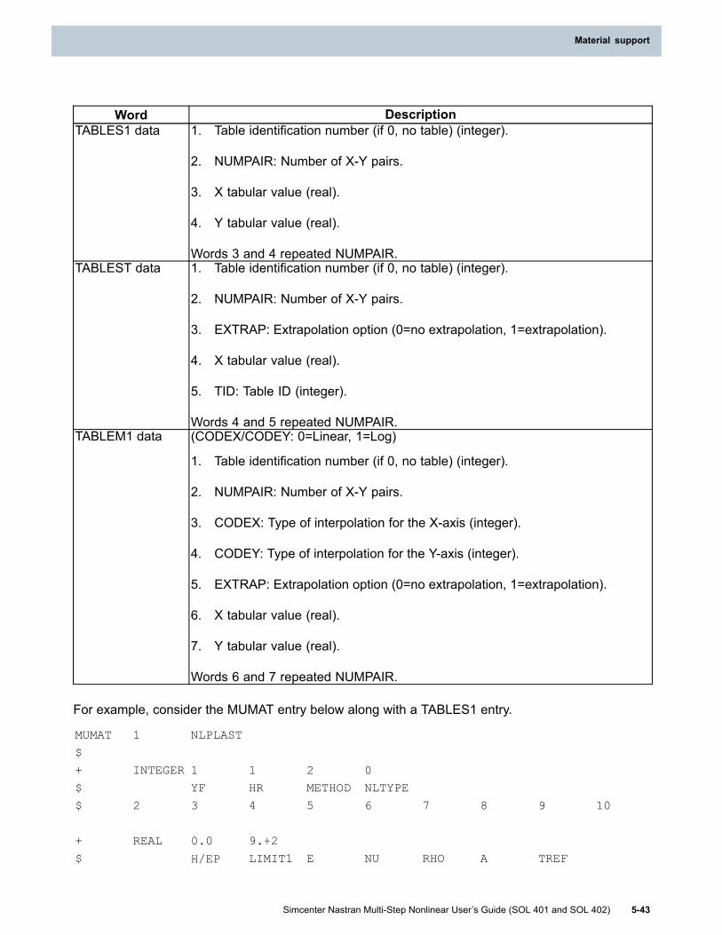
Material support
Word DescriptionTABLES1 data 1. Table identification number (if 0, no table) (integer).
2. NUMPAIR: Number of X-Y pairs.
3. X tabular value (real).
4. Y tabular value (real).
Words 3 and 4 repeated NUMPAIR.TABLEST data 1. Table identification number (if 0, no table) (integer).
2. NUMPAIR: Number of X-Y pairs.
3. EXTRAP: Extrapolation option (0=no extrapolation, 1=extrapolation).
4. X tabular value (real).
5. TID: Table ID (integer).
Words 4 and 5 repeated NUMPAIR.TABLEM1 data (CODEX/CODEY: 0=Linear, 1=Log)
1. Table identification number (if 0, no table) (integer).
2. NUMPAIR: Number of X-Y pairs.
3. CODEX: Type of interpolation for the X-axis (integer).
4. CODEY: Type of interpolation for the Y-axis (integer).
5. EXTRAP: Extrapolation option (0=no extrapolation, 1=extrapolation).
6. X tabular value (real).
7. Y tabular value (real).
Words 6 and 7 repeated NUMPAIR.
For example, consider the MUMAT entry below along with a TABLES1 entry.
MUMAT 1 NLPLAST
$+ INTEGER 1 1 2 0
$ YF HR METHOD NLTYPE
$ 2 3 4 5 6 7 8 9 10
+ REAL 0.0 9.+2
$ H/EP LIMIT1 E NU RHO A TREF
Simcenter Nastran Multi-Step Nonlinear User’s Guide (SOL 401 and SOL 402) 5-43
Material support

Chapter 5: Material support
+ TABLES1 80
TABLES1 80 +
+ 0.0 0.0 7.5-4 9.+2 17.5-4 1.5+327.5-42.0+3 +
+ ENDT
Using the information above, these entries are formatted into the array shown below.
Description MATIN IntegerData MATIR Real Data
1 Length of thearray MUDATAI(1) 38 MUDATAR(1) 0.000000000000000D+000
2 Offset MUDATAI(2) 24 MUDATAR(2) 0.000000000000000D+000
3 MUMATidentifier MUDATAI(3) 2 MUDATAR(3) 0.000000000000000D+000
4 MUMAT data MUDATAI(4) 1 MUDATAR(4) 0.000000000000000D+0005 MUMAT data MUDATAI(5) 2.31E+18 MUDATAR(5) 0.000000000000000D+0006 MUMAT data MUDATAI(6) 2.31E+18 MUDATAR(6) 0.000000000000000D+0007 MUMAT data MUDATAI(7) 0 MUDATAR(7) 0.000000000000000D+0008 MUMAT data MUDATAI(8) 0 MUDATAR(8) 0.000000000000000D+0009 MUMAT data MUDATAI(9) 7 MUDATAR(9) 0.000000000000000D+00010 MUMAT data MUDATAI(10) 2.31E+18 MUDATAR(10) 0.000000000000000D+00011 Code
descriptor
1 = Real data
MUDATAI(11) 1 MUDATAR(11) 0.000000000000000D+000
12 Size of realdata MUDATAI(12) 2 MUDATAR(12) 0.000000000000000D+000
13Value(1) inMUDATARarray
MUDATAI(13) 0 MUDATAR(13) 0.000000000000000D+000
14Value(2) inMUDATARarray
MUDATAI(14) 0 MUDATAR(14) 900
15 Codedescriptor
2 = Integer data
MUDATAI(15) 2 MUDATAR(15) 0.000000000000000D+000
16 Size of Integerdata MUDATAI(16) 4 MUDATAR(16) 0.000000000000000D+000
17 Value(1) MUDATAI(17) 1 MUDATAR(17) 0.000000000000000D+00018 Value(2) MUDATAI(18) 1 MUDATAR(18) 0.000000000000000D+00019 Value(3) MUDATAI(19) 2 MUDATAR(19) 0.000000000000000D+00020 Value(4) MUDATAI(20) 0 MUDATAR(20) 0.000000000000000D+00021 Code
descriptor
3 = Tables1data
MUDATAI(21) 3 MUDATAR(21) 0.000000000000000D+000
5-44 Simcenter Nastran Multi-Step Nonlinear User’s Guide (SOL 401 and SOL 402)
Chapter 5: Material support

Material support
Description MATIN IntegerData MATIR Real Data
22 Number ofTables1
Table IDs
MUDATAI(22) 1 MUDATAR(22) 0.000000000000000D+000
23 Tables1 ID MUDATAI(23) 80 MUDATAR(23) 0.000000000000000D+00024 Code
descriptor
6 = Mappingdata
MUDATAI(24) 6 MUDATAR(24) 0.000000000000000D+000
25 Size ofMapping data MUDATAI(25) 3 MUDATAR(25) 0.000000000000000D+000
26 Table ID MUDATAI(26) 80 MUDATAR(26) 0.000000000000000D+00027 Table Type
3 = Tables1
MUDATAI(27) 3 MUDATAR(27) 0.000000000000000D+000
28 Index toTables1 data MUDATAI(28) 29 MUDATAR(28) 0.000000000000000D+000
29 Tables1 ID MUDATAI(29) 80 MUDATAR(29) 0.000000000000000D+00030 No. of XY pairs MUDATAI(30) 4 MUDATAR(30) 0.000000000000000D+00031 X(1) MUDATAI(31) 0 MUDATAR(31) 0.000000000000000D+00032 Y(1) MUDATAI(32) 0 MUDATAR(32) 0.000000000000000D+00033 X(2) MUDATAI(33) 0 MUDATAR(33) 7.500000000000000D-00434 Y(2) MUDATAI(34) 0 MUDATAR(34) 90035 X(3) MUDATAI(35) 0 MUDATAR(35) 1.750000000000000D-00336 Y(3) MUDATAI(36) 0 MUDATAR(36) 150037 X(4) MUDATAI(37) 0 MUDATAR(37) 2.750000000000000D-00338 Y(4) MUDATAI(38) 0 MUDATAR(38) 2000
Source code examples
Source code examples are included with the Simcenter Nastran installation at the following locations.
• Source code written in C can be found at:installation_location\nxnr\nxumat\democ\
• Source code written in FORTRAN can be found at:installation_location\nxnr\nxumat\demof\
Compiling instructions
The source code examples are located with the installation at the following locations.
• The FORTRAN source code and compile procedures are located at:installation_location\nxnr\nxumat\demof
• The C source code and compile procedures are located at:installation_location\nxnr\nxumat\democ
Simcenter Nastran Multi-Step Nonlinear User’s Guide (SOL 401 and SOL 402) 5-45
Material support

Chapter 5: Material support
The example source code has been tested with the Intel Compiler 13. The resulting .dll for Windowsand the resulting .so for Linux, both generated from this compiler version, have been tested andverified to work with NX Nastran 12. You can use any compiler as long as you adhere to the standardNXUMAT description in the provided source code, and the compiled .dll or .so file uses one of thefollowing handles as entry points:NXUMAT, NXUMAT_, nxumat or nxumat_.
Template make files are provided in the democ and demof folders for both Windows and Linuxoperating systems.
If you run “nmake libumat.dll” in the demof or democ folders on a Windows machine, a Windowsshared library (libnxumat.dll) will be produced from the FORTRAN or C code, respectively.
If you run “make libumat.so” in the demof or democ folders on a Linux machine, a Linux shared library(libnxumat.so) will be produced from the FORTRAN or C code, respectively.
This assumes that you have an Intel Fortran or C compiler, and the nmake or make utility on Windowsor Linux, respectively. You will need to point to proper compilers and linkers in the makefiles tosuccessfully compile.
Ready-to-run routine and test cases
Compiled example routines and Simcenter Nastran input files are included with the SimcenterNastran installation to demonstrate the input file requirements and the general workflow.
• On Windows:Compiled Fortran code: installation_location\nxnr\em64tntl\libnxumat_demofCompiled C code: installation_location\nxnr\em64tntl\libnxumat_democ.dll
• On Linux:Compiled Fortran code: installation_location\nxnr\x86_64linuxl\libnxumat_demof.soCompiled C code: installation_location\nxnr\x86_64linuxl\libnxumat_democ.so
Before using the compiled examples, you will need to follow the instructions in Material library pathto point Simcenter Nastran to a compiled example library. You can point Simcenter Nastran toeither the Fortran or the C compiled example.
Nine material models are included in the compiled example. You can select a specific model in yourSimcenter Nastran input file with the MODNAME1 field on the MUMAT bulk entry.
The following table summarizes the nine material models, the MODNAME1 input definition you use toselect a specific material model, and a ready-to-run Simcenter Nastran input file nxumatex*.dat foreach material model.
You can find the ready-to-run input files at:installation_location\nxnr\nxumat\demodat\
MODNAME1 Input File DescriptionEISO nxumatex1.dat Isotropic, temperature independentEORTHO nxumatex2.dat Orthotropic, temperature independentEANISO nxumatex3.dat Anisotropic, temperature independentETISO nxumatex4.dat Isotropic, temperature dependentETORTHO nxumatex5.dat Orthotropic, temperature dependentETANISO nxumatex6.dat Anisotropic, temperature dependent
5-46 Simcenter Nastran Multi-Step Nonlinear User’s Guide (SOL 401 and SOL 402)
Chapter 5: Material support

Material support
MODNAME1 Input File DescriptionNLPLAST nxumatex7.dat Plasticity, temperature dependentNLCREEP nxumatex8.dat Creep, temperature dependent
PLASCR nxumatex9.dat Plasticity and creep combined, temperaturedependent
CZDAMG nxumatex10.dat Damage model for cohesive elements
EHOOK nxumatex11.dat Hooke's matrix of initial stiffness for solidelements
CZEHOOK nxumatex12.dat Hooke's matrix of initial stiffness forcohesive elements
Material library path
There are three ways, in the following order of precedence, in which you can point Simcenter Nastranto the location of your material library.
• You can define the keyword umatlib on either the command line or in your RCF file. For example,umatlib=D:/scratch/mymaterial.dll
• You can define the environment variable NXN_LOCAL_LIB_NAME. For example,
NXN_LOCAL_LIB_NAME D:/scratch/mymaterial.dll
• If you are run Simcenter Nastran on a Windows machine, you can replace the following file withyour compiled routine:installation_location\nxnr\em64tntl\libnxumat.dll
If you are run Simcenter Nastran on a Linux machine, you can replace the following file with yourcompiled routine:installation_location\nxnr\x86_64linuxl\libnxumat.so
Debugging
You can debug a .dll file using Visual Studio on Windows as long as you build the .dll file with theoptions required for debugging. The .dll file you use for debugging can be built with the make_dll.bator the nmake utility.You can use the following procedure to debug.
1. Simcenter Nastran must be configured so that it reads its input options from a file instead of thecommand line. You will create an *.asg file which contains the configuration options. The *.asgfile will include options such as the input file name, memory settings, and optionally the umatlibkeyword defining the path to the .dll.You can use the following procedure to create an *.asg file.
a. Set the environment variable NXN_NOEXE=1.
set NXN_NOEXE=1
b. Define your Material library path. Run a Simcenter Nastran job using the input file whichincludes your MUMAT bulk entry. When the variable NXN_NOEXE=1 is defined, SimcenterNastran will generate the .asg file and stop. No solution will be performed. The .asg filegenerated will have the name of the input file along with some process id informationappended to it.
Simcenter Nastran Multi-Step Nonlinear User’s Guide (SOL 401 and SOL 402) 5-47
Material support
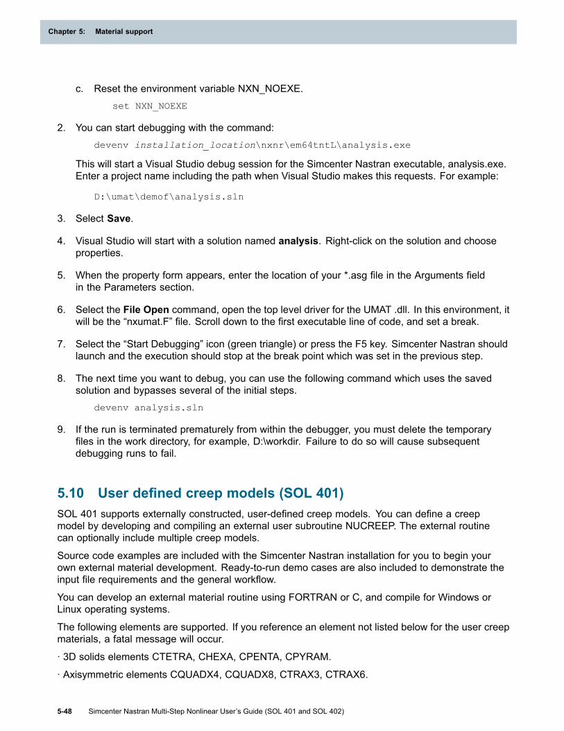
Chapter 5: Material support
c. Reset the environment variable NXN_NOEXE.set NXN_NOEXE
2. You can start debugging with the command:devenv installation_location\nxnr\em64tntL\analysis.exe
This will start a Visual Studio debug session for the Simcenter Nastran executable, analysis.exe.Enter a project name including the path when Visual Studio makes this requests. For example:
D:\umat\demof\analysis.sln
3. Select Save.
4. Visual Studio will start with a solution named analysis. Right-click on the solution and chooseproperties.
5. When the property form appears, enter the location of your *.asg file in the Arguments fieldin the Parameters section.
6. Select the File Open command, open the top level driver for the UMAT .dll. In this environment, itwill be the “nxumat.F” file. Scroll down to the first executable line of code, and set a break.
7. Select the “Start Debugging” icon (green triangle) or press the F5 key. Simcenter Nastran shouldlaunch and the execution should stop at the break point which was set in the previous step.
8. The next time you want to debug, you can use the following command which uses the savedsolution and bypasses several of the initial steps.
devenv analysis.sln
9. If the run is terminated prematurely from within the debugger, you must delete the temporaryfiles in the work directory, for example, D:\workdir. Failure to do so will cause subsequentdebugging runs to fail.
5.10 User defined creep models (SOL 401)SOL 401 supports externally constructed, user-defined creep models. You can define a creepmodel by developing and compiling an external user subroutine NUCREEP. The external routinecan optionally include multiple creep models.
Source code examples are included with the Simcenter Nastran installation for you to begin yourown external material development. Ready-to-run demo cases are also included to demonstrate theinput file requirements and the general workflow.
You can develop an external material routine using FORTRAN or C, and compile for Windows orLinux operating systems.
The following elements are supported. If you reference an element not listed below for the user creepmaterials, a fatal message will occur.
∙ 3D solids elements CTETRA, CHEXA, CPENTA, CPYRAM.
∙ Axisymmetric elements CQUADX4, CQUADX8, CTRAX3, CTRAX6.
5-48 Simcenter Nastran Multi-Step Nonlinear User’s Guide (SOL 401 and SOL 402)
Chapter 5: Material support

Material support
∙ Plane strain elements CPLSTN3, CPLSTN4, CPLSTN6, CPLSTN8.
∙ Plane strain elements that reference the generalized plane strain property (PGPLSN).
∙ Plane stress elements CPLSTS3, CPLSTS4, CPLSTS6, CPLSTS8.
∙ Chocking elements CCHOCK3, CCHOCK4, CCHOCK6, CCHOCK8.
∙ Shell elements CTRIA6, CQUAD8, CTRIAR, CQUADR.
Simcenter Nastran Inputs
The MUCRP bulk entry is available to define the creep coefficients in the Simcenter Nastran input file.Simcenter Nastran passes this data to the NUCREEP routine. The MUCRP entry in your input file isthe trigger Simcenter Nastran uses to call the external routine.
The elements referencing the MUCRP entry material ID will use an associated material law defined inthe user defined material routine NUCREEP. The elements referencing the MUCRP entry must alsoreference general material properties defined with a MAT1, MAT9, or MAT11 entry. The elements canalso reference a plastic material defined with the MATS1 entry.
All of the data defined on the MUCRP entry is also passed to the NUCREEP interface. You caninclude a variety of data types on the MUCRP entry. For example, real, integer, tables and table oftables can all be included.
The following tabular data is supported on the MUCRP entry:
• TABLES1 - This is a collection of real data pairs. You reference the ID of TABLES1 entriesdefined in your Simcenter Nastran input file.
• TABLEM1 - This is a collection of real data pairs. You reference the ID of TABLEM1 entriesdefined in your Simcenter Nastran input file.
• TABLEST - This is a collection of real data values versus table IDs. The table IDs reference othertables with a collection of real data pairs. You reference the ID of TABLEST entries defined inyour Simcenter Nastran input file.
Simcenter Nastran also optionally stores, retrieves, and outputs state variable data computed bythe external routine. For example, stress, creep strain and the time increments for each solutionincrement can be stored as state variables. You define the number of state variables in theNUMSTAT field on the MUMAT entry, and Simcenter Nastran will initialize the appropriate storage.
You can request Nastran to output the state variables using the STATVAR case control command.Regardless of what the data is originally, for example, vector or tensor components, SimcenterNastran outputs all the state variable data as scalar values. The GRID/GAUSS output option is alsoavailable on the STATVAR command.
Note: When you reference TABLES1, TABLEM1, TABLEST entries on the MUCRP entry, SimcenterNastran does no interpolation or extrapolation of the data before passing it to the external routine.
NUCREEP interface
Simcenter Nastran will call the NUCREEP subroutine, which serves as the entry point to the userdefined creep models. You must create a shared library (DLL/SO file) from this routine, which willthen be used by Simcenter Nastran.
Simcenter Nastran Multi-Step Nonlinear User’s Guide (SOL 401 and SOL 402) 5-49
Material support

Chapter 5: Material support
The arguments of NUCREEP are detailed below. Simcenter Nastran expects that the real, integerand character values passed from the argument list are of precision REAL*8, INTEGER*8 andCHARACTER (LEN=8).
SUBROUTINE NUCREEP(& D_EFF_CR_SN, D_EFF_SW_SN, STATEVAR , ENG_RATE,& EFF_CR_SN , EFF_SW_SN , PRESS_EQV, STRESS_EQV,& TEMPER_T1 , D_TEMPER ,& TIME_T1 , D_TIME , MOD_NAME1, MOD_NAME2,& INTG_MTHD , INCRM_END , COORD_XYZ, NUM_SV ,& INT_VALS , REAL_VALS , MUDATAI , MUDATAR ,& IOPER , IRET )
D_EFF_CR_SN(5): (Output, Array)Increment of effective creep strain, and its derivatives (derivatives needed when INTG_MTHD=1)
D_EFF_CR_SN(1): increment of effective creep strain.
D_EFF_CR_SN(2):
D_EFF_CR_SN(3):
D_EFF_CR_SN(4):
D_EFF_CR_SN(5):
D_EFF_SW_SN(5): (Output, Array) **Currently not used**Increment of effective swelling strain, and its derivatives
STATEVAR(NUM_SV): (Input/Output, Array)An array of state variables that you specify. It contains the state variables from the previous time stepas input and can be updated with current state variables upon convergence. The length of the arrayis NUM_SV which is defined on the MUCRP entry.
ENG_RATE: (Input/Output, Real) **Currently not used**Magnitude of strain energy rate density
EFF_CR_SN(2): (Input, Array)Effective creep strain
EFF_CR_SN(1): effective creep strain at start of the time increment
EFF_CR_SN(2): effective creep strain at end of the time increment
EFF_SW_SN(2): (Input, Array) **Currently not used**Effective swelling strain
5-50 Simcenter Nastran Multi-Step Nonlinear User’s Guide (SOL 401 and SOL 402)
Chapter 5: Material support

Material support
PRESS_EQV: (Input, Real)
Pressure stress
STRESS_EQV: (Input, Real)
von Mises effective stress
TEMPER_T1: (Input, Real)
Temperature at the end of the time increment
D_TEMPER: (Input, Real)
Increment of temperature
TIME_T1: (Input, Real)
Step time at the end of the time increment
D_TIME: (Input, Real)
Time increment
MOD_NAME1: (Input, Character)
User specified model name, no more than 8 characters
MOD_NAME2: (Input, Character)
User specified model name, no more than 8 characters
INTG_MTHD: (Input, Integer)
Time integration method (0: EXPLICIT, 1: IMPLICIT)
INCRM_END: (Input, Integer)
Flag indicating whether it is the start or the end of the time increment (0: start of increment, 1:end of increment)
COORD_XYZ(3): (Input, Array)
Coordinates of the point, 3 components represent X, Y, Z, respectively
NUM_SV: (Input, Integer)
Number of user-defined state variables
INT_VALS(*): (Input, Array)
Solution values for information (integer)
INT_VALS(1): element ID
INT_VALS(2): Gauss/grid ID
INT_VALS(3): number of step
INT_VALS(4): internal iteration count
INT_VALS(5): subcase ID
INT_VALS(6): (not used)
INT_VALS(7): convergence flag
Simcenter Nastran Multi-Step Nonlinear User’s Guide (SOL 401 and SOL 402) 5-51
Material support

Chapter 5: Material support
REAL_VALS(*): (Input, Array)
Solution values for information (real)
REAL_VALS(1): element thickness
REAL_VALS(2): integration weight
REAL_VALS(3): converter to absolute temperature
MUDATAI(*): (Input, Array)
Material parameters from MUCRP card (integer)
MUDATAR(*): (Input, Array)
Material parameters from MUCRP card (real)
IOPER: (Input, Integer)
Flag of solution process step (0: loading 1: initialization 2: computation)
Only IOPER=2 is activated in this release
IRET: (Output, Integer)
Return value for error check (0: no error)
Build instructions
Before you use the user-defined creep models defined in NUCREEP, you must build your ownshared library to create a *.dll file on Windows or an .so file on Linux. Simcenter Nastran will link tothis shared library for data exchange. You will need to have the Fortran or C compiler to compile thecorresponding source code.
There are demo input files and user subroutines located in the installation folder of Simcenter Nastran.The locations of these files are listed below in "Demo creep models and cases." Once your makefileis correctly defined and your compiler is configured, a shared library of user defined creep modelscan be built. The table below lists the build commands and shared libraries for Windows and Linux.
Platform Build Command Shared LibraryWindows nmake libucreep.dll libucreep.dllLinux make libucreep.so libucreep.so
Specifying the user creep library
Simcenter Nastran looks for the user-defined creep library at a location that you specified on thecommand line or by an environment variable, in that order:
• Define the keyword ucrplib on either the command line or in your RCF file. For example,
ucrplib=D:/workdir/libucreep.dll
• Define the environment variable NXN_UCREEP_LIB. For example,
set NXN_UCREEP_LIB=D:/workdir/libucreep.dll
5-52 Simcenter Nastran Multi-Step Nonlinear User’s Guide (SOL 401 and SOL 402)
Chapter 5: Material support

Material support
Demo creep models and cases
There are five ready-to-run, pre-compiled demonstration models. The table below summarizesthese models.
No. Model Name Input File Description Formulation
1 NLCREEP u401c01.dat
Norton-Bailey,with temperaturedependent materialparameters
2 STRNHARD u401sth.dat Strain Hardening
3 NORTON u401c01nt.dat Norton
4 GENGAROF u401c01ga.dat GeneralizedGarofalo
5 GENBLACK u401c01bb.dat GeneralizedBlackburn
The demonstration models are available in the Simcenter Nastran installation folder as shown below.Note that all of the models are integrated into a single library.
On Windows
Compiled Fortran code: installation_location\scnas\em64tntl\libucreep_ucrpf.dll
Compiled C code: installation_location\scnas\em64tntl\libucreep_ucrpc.dll
On Linux
Compiled Fortran code: installation_location\scnas\x86_64linuxl\libucreep_ucrpf.so
Compiled C code: installation_location\scnas\x86_64linuxl\libucreep_ucrpc.so
5.11 Disable plasticity and creepThe MATNL parameter allows you to switch all creep and/or plasticity effects on/off for all relatedelements.
Disable plasticity and creep in SOL 401
In SOL 401, when the MATNL parameter is set to 1 (PARAM,MATNL,1) to turn on creep and/orplasticity effects, the MATOVR bulk entry lets you optionally disable the creep and plasticity effects forthe elements of a selected GROUP bulk entry.
• Use TYPE = "ELEM" to reference a GROUP bulk entry that includes a list of elements. TheMATOVR specification applies to the listed elements.
• Use TYPE = "PROP" to reference a GROUP bulk entry that includes a list of properties. TheMATOVR specification applies to all elements that reference the properties listed in the GROUPbulk entry.
For more information, see the MATOVR bulk entry in the Simcenter Nastran Quick Reference Guide.
Simcenter Nastran Multi-Step Nonlinear User’s Guide (SOL 401 and SOL 402) 5-53
Material support

Chapter 5: Material support
Disable plasticity and creep in SOL 402
In SOL 402, when the MATNL parameter is set to 1 (PARAM,MATNL,1) to turn on creep and/orplasticity effects, you can turn them off at the subcase level. Use CREEP,NO to exclude creep effectsand/or PLASTIC,NO to exclude plastic effects.
Note
If PARAM,MATNL is set to -1 (all material nonlinearities disabled), you cannot use theCREEP,YES or PLASTICITY,YES in a subcase to enable creep or plasticity effects inthat subcase.
Note
Creep and plasticity effects are enabled or disabled for all the elements that can supportthem. You cannot enable or disable these effects for a specific group of elements.
For more information, see the NLCNTL2 bulk entry in the Simcenter Nastran Quick Reference Guide.
5.12 Hyperelastic materials (SOL 402)Hyperelastic models are popular for modeling the large strain nonlinear behavior of incompressiblematerials, such as rubber.
These models do not provide any special insight into material behavior. They are based on thedefinition of the strain energy density as a function of on strain invarients or stretch ratios. The inputof the models are coefficients that are mainly obtained by curve-fits of test data.
In SOL 402, you can use the MATHE bulk entry to define the following hyperelastic materials:Mooney-Rivlin, Ogden, and Hyperfoam.
Note
The Arruda-Boyce model and the Sussman-Bathe model are not supported in SOL 402.
You can also add viscoplacity effects to these materials with the MATHEV bulk entry and add Mullineffects with the MATHEM bulk entry.
Mooney-Rivlin materials: the MATHE bulk entry
Mooney-Rivlin materialThe generalized Mooney-Rivlin strain energy function can be expressed as follows:
with
5-54 Simcenter Nastran Multi-Step Nonlinear User’s Guide (SOL 401 and SOL 402)
Chapter 5: Material support

Material support
where:
• is the deviatoric stretch ratio defined as:
• K and J are the bulk modulus and volume ratio, respectively.
If you do not provide K, the software uses a default value of 1000(C10+C01).
SOL 402 requires the linearized Poisson coefficient to be positive. The linearized Poisson coefficientNu is computed based on the bulk modulus K and the two first material constants C10 and C01 using:
Odgden materials: the MATHE bulk entry
For the Ogden material model, the strain energy function is:
where:
• μk and αk are material constants.
• is the deviatoric stretch ratio defined as:
,
• K and J are the bulk modulus and volume ratio, respectively.
K is defined as:
Hyperfoam materials: the MATHE bulk entry
For the hyperfoam material model, the strain energy function is:
Simcenter Nastran Multi-Step Nonlinear User’s Guide (SOL 401 and SOL 402) 5-55
Material support

Chapter 5: Material support
where:
• μk, αk and βk are material constants.
• J is the volume ratio.
The hyperfoam material model in SOL 402 does not use the bulk modulus K.
For more information about these hyperelastic materials, see the MATHE bulk entry in the SimcenterNastran Quick Reference Guide.
Mooney-Rivlin alternative: the MATHP bulk entry
The MATHP bulk entry is an alternative to MATHE card to define a hyperelastic material based onMooney model.
It allows you to define the strain potential directly by providing the Mooney coefficients or by using theexperimental data provided in the TABi parameters of the MATHP bulk entry.
If experimental data are provided, the Mooney coefficients are computed internally with a fittingprocedure.
The generalized Mooney-Rivlin strain energy function can be expressed as follows:
where:
• and are the first and second distortional strain invariants, respectively.
• J=det F is the determinant of the deformation gradient.
• 2D1=K and 2(A10 + A01)=G at small strains, in which K is the bulk modulus and G is the shearmodulus.
The model reduces to a Mooney-Rivlin material if NA=3.
• T is the current temperature and T0 is the initial temperature.
In SOL 402, the degree of the Mooney-Rivlin strain potential is limited to 4 for the distortional part,to 1 for the volumetric part.
SOL 402 requires the linearized Poisson coefficient to be positive. The linearized Poisson coefficientNu is computed based on the volumetric coefficient D1 and the two first distortional constants A10and A01.
5-56 Simcenter Nastran Multi-Step Nonlinear User’s Guide (SOL 401 and SOL 402)
Chapter 5: Material support

Material support
For more information, see the MATHP bulk entry in the Simcenter Nastran Quick Reference Guide.
Adding viscoplasticty effects to hyperelastic materials: the MATHEV bulk entry
The viscoelastic effect in the hyperelastic material is based on Prony series.
For more information, see the MATHEV bulk entry in the Simcenter Nastran Quick Reference Guide.
Adding Mullin effects to hyperelastic materials: the MATHEM bulk entry
The Mullins effect in the hyperelastic matMooney-Rivlinstrainenergyfunctionerials is based on theOgden-Roxburgh model and takes damages in elastomers into account.
When material is unloaded, the stress-strain curve is below the initial curve. When material is loadedagain, it follows the unloading path.
In this example:
1. The curve 0 A1 A2 A3 is the initial loading curve without taking into account Mullins effect.
2. When material is loaded up to A1 and then unloaded, it follows path A1 B1 0. When it is loadedagain up to A2, it follows path 0 B1 A1 A2.
3. If it is unloaded and the reloaded, it follows path A2 B2 0 B2 A2 A3.
4. And so on.
For more information, see the MATHEM bulk entry in the Simcenter Nastran Quick Reference Guide.
Simcenter Nastran Multi-Step Nonlinear User’s Guide (SOL 401 and SOL 402) 5-57
Material support
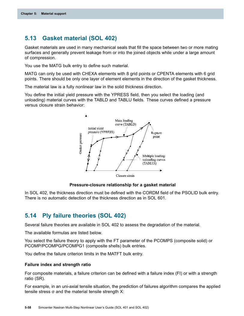
Chapter 5: Material support
5.13 Gasket material (SOL 402)Gasket materials are used in many mechanical seals that fill the space between two or more matingsurfaces and generally prevent leakage from or into the joined objects while under a large amountof compression.
You use the MATG bulk entry to define such material.
MATG can only be used with CHEXA elements with 8 grid points or CPENTA elements with 6 gridpoints. There should be only one layer of element elements in the direction of the gasket thickness.
The material law is a fully nonlinear law in the solid thickness direction.
You define the initial yield pressure with the YPRESS field, then you select the loading (andunloading) material curves with the TABLD and TABLU fields. These curves defined a pressureversus closure strain behavior:
Pressure-closure relationship for a gasket material
In SOL 402, the thickness direction must be defined with the CORDM field of the PSOLID bulk entry.There is no automatic detection of the thickness direction as in SOL 601.
5.14 Ply failure theories (SOL 402)Several failure theories are available in SOL 402 to assess the degradation of the material.
The available formulas are listed below.
You select the failure theory to apply with the FT parameter of the PCOMPS (composite solid) orPCOMP/PCOMPG/PCOMPG1 (composite shells) bulk entries.
You define the failure criterion limits in the MATFT bulk entry.
Failure index and strength ratio
For composite materials, a failure criterion can be defined with a failure index (FI) or with a strengthratio (SR).
For example, in an uni-axial tensile situation, the prediction of failures algorithm compares the appliedtensile stress σ and the material tensile strength X:
5-58 Simcenter Nastran Multi-Step Nonlinear User’s Guide (SOL 401 and SOL 402)
Chapter 5: Material support

Material support
• The failure index FI is defined as σ / X. Failure occurs once the failure index has a value of 1or above.
• To know the strength ratio SR by which the stress σ can be multiplied to produce failure (FI = 1):
1 = (SR * σ ) / X.
Then, SR = X / σ.
A simple relationship between the failure index and the strength ratio can be computed as:
SR = 1 / FI.
You control the computation of the ply strength ratios with the PARAM,SRCOMPS parameter:
• When PARAM,SRCOMPS,YES, ply strength ratios are output for composite elements that havethe failure indices requested.
• For shell composites, when PARAM,SRCOMPS,YES, the software computes both the failureindex and the strength ratio.
• For solid composites, when PARAM,SRCOMPS,YES, the software only computes the strengthratio,and not the failure index.
Tsai-Hill theory
where X, Y, and Z are, either the tensile or compressive strength values, depending on the sign of theσ1, σ2, and σ3 stress components.
The software automatically makes the choice:
• σ1 >=0, X = XT.
σ1 <0, X = XC.
(with T for traction and C for compression).
• σ2 >=0, Y = YT.
σ2 <0, Y = YC.
• σ3 >=0, Z = ZT.
σ3 <0, Z = ZC.
Note
The shear strength values R, S, and T are always positive.
Hoffman theory
In the Hoffman criterion, the same formulation is used for volume, shell, and membrane elements.
Simcenter Nastran Multi-Step Nonlinear User’s Guide (SOL 401 and SOL 402) 5-59
Material support

Chapter 5: Material support
The formula only takes the in-plane stress components into account, so it is independent of theout-of-plane stress components.
where:
• σi are stresses and τij are shear stresses.
• XT and YT are the tensile strength values.
• XC and YC are the compressive strength values.
• The shear strength value R is always positive.
Tsai-Wu theory
In the Hoffman criterion, the same formulation is used for volume, shell, and membrane elements.
The formula only takes the transverse stress components into account in shells.
where:
• σi are stresses and τij are shear stresses.
• XT, YT, and ZT are the tensile strength values.
• XC, YC, and ZC are the compressive strength values.
• The shear strength values R, S, and T are always positive.
• The F12, F23, and F13 are interactions terms.
Maximum strain theory
In the maximum total strain theory, the software compares each of the total strain tensor componentsindependently with their maximum allowable value.
The total strains are used, including the mechanical strains and the thermal strains.
The six components that will be tested are:
5-60 Simcenter Nastran Multi-Step Nonlinear User’s Guide (SOL 401 and SOL 402)
Chapter 5: Material support

Material support
where:
• εi are strains, ɣij are shear strains.
• DTij are the limits in traction, DCij the limits in compression, and DSTij the shear limits.
Maximum stress theory
In the maximum stress theory, the software compares each of the stress tensor componentsindependently with their maximum allowable value.
The six components that will be tested are:
where:
• σi are stresses and τij are shear stresses.
• XT, YT, and ZT are the tensile strength values.
• XC, YC, and ZC are the compressive strength values.
• R, S, and T are the shear strength values.
Maximum transverse shear theory
In the maximum transverse theory, the software compares each of the transverse shear stresscomponents independently with their maximum allowable value.
The two shear components that will be tested are:
|τ23| < S
and
|τ13| < T
Simcenter Nastran Multi-Step Nonlinear User’s Guide (SOL 401 and SOL 402) 5-61
Material support

Chapter 5: Material support
where the shear strength values S and T are always positive.
For more information, see the Ply failure criteria theories in the Samcef documentation.
5-62 Simcenter Nastran Multi-Step Nonlinear User’s Guide (SOL 401 and SOL 402)
Chapter 5: Material support
Chapter 6: Boundary conditions
6.1 ConstraintsIn the Case Control section, an SPC entry is used to select a single point constraint set (s-set) whichwill be applied to the structural model. The specified set identification must be identical to the SIDfield of an SPC, SPC1 or SPCADD bulk entry. Notice that SPCADD entries take precedence overSPC or SPC1 entries. If both have the same SID, only the SPCADD entry will be used.
A significant application of SPC is the imposition of boundary conditions. The PS field in the GRIDentry is also able to specify single-point constraints associated with a grid point. Although, theseconstraints are so-called permanent constraints which can not be changed during the analysis. Anadvantage of using SPC to specify boundary conditions is that these boundary conditions can bechanged from subcase to subcase by selecting a different SPC set inside each subcase.
SPC input summary
• The SPC=n case control command selects either the SPC, SPC1, or SPCADD bulk entry.
The SPC condition can change between subcases.
The SPC entry can optionally be used to define a time-unassigned enforced displacement. Itcannot be defined as time-assigned. That is, it cannot be selected with the EXCITEID on theTLOAD1 entry. For a time-assigned enforced displacement, you can use the SPCD entry. SeeMechanical Loads for information on the SPCD entry.
The SPCFORCES case control command is supported to request the SPC force output.
6.2 Multipoint constraintWhile a single point constraint (SPC) is used to constrain the motion of a degree-of-freedom,a multipoint constraint (MPC) is used to tie the motion of one degree-of-freedom to otherdegrees-of-freedom. The MPC command in the Case Control section is used to select a multipointconstraint set in the Bulk Data. The specified MPC set identification must appear at least in oneMPC or MPCADD bulk entry. Each MPC bulk entry may be used to define a constraint equationinvolving a group of degrees-of-freedom in which the first degree-of-freedom is assumed to be thedependent degree-of-freedom and included in the m-set. All the degree-of-freedom in m-set will becondensed out prior to the matrix operations. Their response will be directly recovered from those ofthe independent degrees-of-freedom according to the specified constraint equation. MPC conditionscan change from subcase to subcase.
MPC input summary
• The MPC=n case control command selects either the MPC or MPCADD bulk entry.
MPC conditions can change between subcases.
MPCs do not update for large displacements (PARAM,LGDISP,1).
Simcenter Nastran Multi-Step Nonlinear User’s Guide (SOL 401 and SOL 402) 6-1

Chapter 6: Boundary conditions
6.3 Enforced displacementsEnforced displacements may be specified in the Bulk Data section using SPC or SPCD entries. AnSPC can be used to define time-unassigned enforced displacements. An SPCD can be used todefine time-assigned or time-unassigned enforced displacements. See Boundary conditions andMechanical Loads for input details.
Each SPC entry may define enforced displacements for up to two grid or scalar points. Several SPCentries which reference the same SID may be used if enforced displacements for more than two gridor scalar points are desired. The only disadvantage of this method is that the entire s-set must beredefined if the enforced displacement conditions vary among subcases.
If a time-assigned or time-unassigned enforced displacement condition is defined with the SPCDentry, a constraint must also be defined with the SPC entry on the same DOF referenced by theSPCD entry.
If multiple enforced displacement conditions are applied to the same DOF, the software uses thefollowing precedence.
• A time-assigned enforced displacement defined with the SPCD entry, which is referenced bythe EXCITEID on the TLOAD1 entry, will overwrite time-unassigned enforced displacementsdefined with the SPCD or SPC entries.
• A time-unassigned enforced displacement defined with the SPCD entry, which is referenced bythe LOAD=n case control command, will overwrite a time-unassigned enforced displacementdefined with the SPC entry.
6-2 Simcenter Nastran Multi-Step Nonlinear User’s Guide (SOL 401 and SOL 402)
Chapter 6: Boundary conditions

Chapter 7: Loads
7.1 Loads overviewThe solution strategy in nonlinear is to apply the loads in an incremental fashion until the desired loadlevel is reached. The algorithms remember the loads from one subcase to the next.
The methods employed to define loads in SOL 401 and SOL 402 are similar to those used in atime history solutions. A single degree-of-freedom or a set of GRID points may be loaded withforce pattern that varies with time. Functions may be tabular such as an earthquake or a boosterliftoff, or they may be simple analytic functions such as a sine wave. Simple static load sets may beused to create the dynamic loads. They may be scaled and combined with other loads to simulatecomplex loading problems.
Time history loads define the loadings as functions of time and the location. They can be a loadapplied at a particular degree-of-freedom, pressure over the surface area, or the body force simulatingan acceleration. The time history is provided by TLOADi bulk entry.
7.2 Mechanical loads (SOL 401)Mechanical loads can be defined in SOL 401 as time-assigned or time-unassigned. SOL 401 is astatic solution, and time is only used as the mechanism to increment loads. Time-assigned andtime-unassigned loads can be combined in the same static subcase.
• Load selection in Case Control:
o Time-unassigned loads are selected with the LOAD case control command,
LOAD=n
where n points to a DAREA, FORCDST, FORCE, FORCE1, FORCE2, GRAV, MOMENT,MOMENT1, MOMENT2, PLOAD, PLOAD1, PLOAD2, PLOAD4, PLOADE1, PLOADFP,PLOADX1, RFORCE, RFORCE1, SLOAD, SPCD, or LOADSET entry.
The LVAR parameter on the NLCNTL bulk entry controls if time-unassigned mechanical loadsare ramped (default), or not ramped for each subcase. The ramping helps convergence byreducing the load increments. You can optionally turn the ramping off by setting LVAR=STEPon the NLCNTL bulk entry.
o Time-assigned loads are selected with the DLOAD case control command,
DLOAD=n
where n points to a load set defined by a TLOAD1 bulk entry, or a DLOAD bulk entry if youwant to combine multiple TLOAD1 entries into a single load set.
• Time-assigned load definition in Bulk Data:
o TLOAD1 or TLOAD3 - Defines time-assigned loads.
Simcenter Nastran Multi-Step Nonlinear User’s Guide (SOL 401 and SOL 402) 7-1

Chapter 7: Loads
TLOAD1 is used to define most time-assigned loads. See Defining the TLOAD1 entrybelow. The exception is the distributed force defined with the FORCDST bulk entry.
TLOAD3 is only used to select the FORCDST bulk entry to define a time-assigned distributedforce. See Distributed force to a surface or edge.
o TABLEDi (i=1,2,3,4) - Table that defines the load variation with time.
o DLOAD - Combines several TLOAD1 and TLOAD3 entries.
• Defining the TLOAD1 entry:
o The EXCITEID field on the TLOAD1 entry selects the static load set IDs.
o The supported static load inputs are the DAREA, FORCE, FORCE1, FORCE2, GRAV,MOMENT, MOMENT1, MOMENT2, PLOAD, PLOAD1, PLOAD2, PLOAD4, PLOADE1,PLOADX1, RFORCE, RFORCE1, SLOAD, and SPCD bulk entries.
o The TYPE field on the TLOAD1 entry should be “0” for all load inputs selected by theEXCITEID field, except for the SPCD entry. The SPCD entry requires “1” in the TYPE field.
o A real value is supported in the DELAY field on a TLOAD1 entry to optionally shift the timesteps used to compute the associated loads.
o A temperature load cannot be selected on the EXCITEID field. See Thermal Loads.
o The TID field selects a TABLEDi, which defines a load scaling versus time function.
o The figure below demonstrates how the DLOAD, TLOAD1, FORCE (for example), andTABLEDi bulk entries relate to one another.
o Load Input Example 1:
When there is more than one time-assigned load set, the DLOAD bulk entry is required:
$2345678$2345678$2345678$2345678$2345678$2345678$2345678$2345678$2345678$$ DLOAD COMBINES MULTIPLE TLOAD1 (102 AND 105)DLOAD 17 1. 1. 102 1. 105$$ TIME-ASSIGNED FORCE, EXCITEID=125, TYPE=0 (DEFAULT), TIME FUNCTION TID=13TLOAD1 102 125 13
7-2 Simcenter Nastran Multi-Step Nonlinear User’s Guide (SOL 401 and SOL 402)
Chapter 7: Loads

Loads
$FORCE 125 80 0 1. 3. 0. 0.$$ TIME FUNCTION 13 USED FOR FORCE LOADTABLED2 13 0. ++ 0. 0. 1. 100. 2. 0. ENDT$$ TIME-ASSIGNED FORCE EXCITEID=3, TYPE=0 (DEFAULT), TIME FUNCTION TID=12TLOAD1 105 3 1 12$FORCE 3 73 0 2. 8. 0. 0.$$ TIME FUNCTION 12 USED FOR FORCE LOADTABLED2 12 0. ++ 0. 0. 2. 1. ENDT
o Load Input Example 2:
When there is only one time-assigned load set, the DLOAD entry is not required:
$2345678$2345678$2345678$2345678$2345678$2345678$2345678$2345678$2345678$$ TIME-ASSIGNED FORCE, EXCITEID=125, TYPE=0 (DEFAULT), TIME FUNCTION TID=13TLOAD1 102 125 13$FORCE 125 80 0 1. 3. 0. 0.PLOAD 125 100.0 21 30 18 10PLOAD 125 100.0 10 18 22 25$$ TIME FUNCTION 13 USED FOR LOADTABLED2 13 0. ++ 0. 0. 1. 100. 2. 0. ENDT$
• Additional Information about mechanical loads:
o Enforced displacements may be specified using SPC or SPCD entries. See Enforceddisplacements.
o Loads in any subcase are total loads as opposed to incremental loads from the previoussubcase. In other words, the ending load from a previous subcase does not become theinitial loading for the consecutive subcase.
o If no load is applied in a subcase, the total load is zero.
o LOAD=n or DLOAD=n defined at the global level is used in all statics subcases unlessa different LOAD=n or DLOAD=n is defined in a subcase.
o If a time-assigned and time-unassigned enforced displacement condition is defined withthe SPCD entry, a constraint must also be defined with the SPC entry on the same DOFreferenced by the SPCD entry.
Simcenter Nastran Multi-Step Nonlinear User’s Guide (SOL 401 and SOL 402) 7-3
Loads

Chapter 7: Loads
o The TSTEP1 bulk entry defines the time step intervals in which a solution will be generatedand output in a static subcase. If your time steps defined by the TSTEP1 entry exceed thetime values defined in your TABLEDi entry, by default, the software will extrapolate the datadefined in the TABLEDi entry. The software will issue a warning if extrapolation occurs. Ifyou do not want the software to extrapolate the data, you can enter “1” in the EXTRAPfield on the TABLEDi entry.
o The LOADOFF parameter is available on the NLCNTL bulk entry to turn ON or OFFcategories of mechanical loads. The NLCNTL entry can be defined in the global subcaselevel and in individual subcases.
The LOADOFF options are as follows.
LOADOFF value ResultLOADOFF=NONE(Default) No loads are turned off.
LOADOFF=BODY Turns off body loads defined with the GRAV, RFORCE, RFORCE1,ACCEL, and ACCEL1 bulk entries.
LOADOFF=BOUNDRY
Turns off boundary loads defined with the PLOAD, PLOAD1,PLOAD2, PLOAD4, PLOADE1, PLOADX1, FORCDST, FORCE,FORCE1, FORCE2, MOMENT, MOMENT1, MOMENT2, andSLOAD bulk entrires.
LOADOFF=BOTH
Turns off both the BODY and BOUNDRY loads listed above.
When LOADOFF=BOTH is defined, the loads which remain oninclude temperature loads, initial stress/strain, strains computedfrom a bolt preload subcase, enforced displacements, and loads asa result of contact conditions.
Note
When running SOL 401 in a Simcenter thermal-structural multiphysics analysis,some mechanical loads such as RFORCE1 are used by both the structural andthermal solutions. It's important to understand that the LOADOFF parameter isonly turning loads on or off for the Simcenter Nastran structural solution, and notthe thermal solution. In addition, the thermal solution can compute pressure loadswhich are then applied in the structural solution. These pressure loads are appliedusing the PLOADi entries, and as a result, they will be turned off from the structuralsolution when LOADOFF=BOUNDRY is defined.
o When you define the RFORCE or RFORCE1 bulk entries as either time-assigned, or as
time-unassigned and ramped, the software uses time to scale the angular velocity and
acceleration , which are used to compute the inertia force.
The time variation is defined either by a time-assigned load referenced by theDLOAD=n case control command, or by a time-unassigned load referenced by the LOAD=ncase control command which is ramped. This ramping is requested with the LVAR parameteron the NLCNTL bulk entry.
The angular velocity is computed as:
7-4 Simcenter Nastran Multi-Step Nonlinear User’s Guide (SOL 401 and SOL 402)
Chapter 7: Loads

Loads
where,
is the rotation vector defined on the RFORCEi entry,
and A is the scale factor of the angular velocity in revolutions per unit time defined on theRFORCEi entry.
The associated force is computed as:
where,
m is the mass computed at each grid point Gi,
and ri and ra are position vectors (not related to the rotation vector). See the remarks on theRFORCEi entries for a definition of the position vectors.
The RFVAR parameter changes how the software interpolates the time variation.
■ When RFVAR=OMEGA (default), the software interpolates the time variation using
.
As a result, if a linear time variation is defined, the angular velocity will vary linearly.
Since is squared in the force computation, the force will not vary linearly.
■ When RFVAR=FORCE, the software interpolates the time variation using .The software then takes the square root of the interpolated value before appling it theangular velocity.
As a result, if a linear time variation is defined, the force will vary linearly, but will not.
Note that the RFVAR parameter setting only changes the interpolation for angular velocity,and not the angular acceleration. Since the angular acceleration is not squared in the forcecomputation, it varies linearly with the force.
For example, if solution times are defined from 0.0 to 1.0 second in 5 increments, at time=0.0,f(t)=0.0, and at time=1.0, f(t)=2.0.
Assume A=1.0, m is an identity matrix,
and , where is a unit vector.
The following table shows the resulting values of and for this simplified input scenario.
RFVAR=OMEGA RFVAR=FORCE
Time
0.0 0.0 0.0 0.0 0.0
Simcenter Nastran Multi-Step Nonlinear User’s Guide (SOL 401 and SOL 402) 7-5
Loads

Chapter 7: Loads
RFVAR=OMEGA RFVAR=FORCE
Time
0.2 0.4 0.16 0.894427 0.80.4 0.8 0.64 1.264911 1.60.6 1.2 1.44 1.5491933 2.40.8 1.6 2.56 1.788854 3.21.0 2.0 4.0 2.0 4.0
7.3 Mechanical loads (SOL 402)Mechanical loads can be defined in SOL 402 as time-assigned or time-unassigned. SOL 402 is asolution supporting static, dynamic, and preload subcases—time is only used as the mechanismto increment loads. Time-assigned and time-unassigned loads can be combined in the samestatic subcase.
• Load selection in Case Control:
o Time-unassigned loads are selected with the LOAD case control command:
LOAD=n
where n points to FORCE, FORCE1, FORCE2, GRAV, MOMENT, MOMENT1, MOMENT2,PLOAD, PLOAD1, PLOAD2, PLOAD4, PLOADE1, PLOADFP, PLOADX1, RFORCE,RFORCE1, or SPCD entry.
The LVAR parameter on the NLCNTL2 bulk entry controls whether time-unassignedmechanical loads are ramped (default) or not for each subcase. Ramping helps convergenceby reducing the load increments. You can optionally turn the ramping off by settingLVAR=STEP on the NLCNTL2 bulk entry.
o Time-assigned loads are selected with the DLOAD case control command:
DLOAD=n
where n points to a load set defined by a TLOAD1 bulk entry, or a DLOAD bulk entry if youwant to combine multiple TLOAD1 entries into a single load set.
• Time-assigned load definition in Bulk Data:
o TLOAD1 - Defines time-assigned loads.
TLOAD1 is used to define most time-assigned loads. See Defining the TLOAD1 entry below.
o TABLEDi (i=1,2,3,4) - Table that defines the load variation with time.
o DLOAD - Combines several TLOAD1 entries.
• Defining the TLOAD1 entry:
o The EXCITEID field on the TLOAD1 entry selects the load set IDs.
7-6 Simcenter Nastran Multi-Step Nonlinear User’s Guide (SOL 401 and SOL 402)
Chapter 7: Loads

Loads
o The supported static load inputs are the FORCE, FORCE1, FORCE2, GRAV, MOMENT,MOMENT1, MOMENT2, PLOAD, PLOAD1, PLOAD2, PLOAD4, PLOADE1, PLOADX1,RFORCE, RFORCE1, and SPCD bulk entries.
o The TYPE field on the TLOAD1 entry should be “0” for all load inputs selected by theEXCITEID field, except for the SPCD entry. The SPCD entry requires “1” in the TYPE field.
o The DELAY field on a TLOAD1 entry is ignored.
o A temperature load cannot be selected on the EXCITEID field. See Thermal Loads.
o The TID field selects a TABLEDi, which defines a load scaling versus time function.
o The figure below demonstrates how the DLOAD, TLOAD1, FORCE (for example), andTABLEDi bulk entries relate to one another.
o Example 1 - Load Input
When there is more than one time-assigned load set, the DLOAD bulk entry is required:
$2345678$2345678$2345678$2345678$2345678$2345678$2345678$2345678$2345678$$ DLOAD COMBINES MULTIPLE TLOAD1 (102 AND 105)DLOAD 17 1. 1. 102 1. 105$$ TIME-ASSIGNED FORCE, EXCITEID=125, TYPE=0 (DEFAULT), TIME FUNCTION TID=13TLOAD1 102 125 13$FORCE 125 80 0 1. 3. 0. 0.$$ TIME FUNCTION 13 USED FOR FORCE LOADTABLED2 13 0. ++ 0. 0. 1. 100. 2. 0. ENDT$$ TIME-ASSIGNED FORCE EXCITEID=3, TYPE=0 (DEFAULT), TIME FUNCTION TID=12TLOAD1 105 3 1 12$FORCE 3 73 0 2. 8. 0. 0.$$ TIME FUNCTION 12 USED FOR FORCE LOADTABLED2 12 0. ++ 0. 0. 2. 1. ENDT
Simcenter Nastran Multi-Step Nonlinear User’s Guide (SOL 401 and SOL 402) 7-7
Loads

Chapter 7: Loads
o Example 2- Load Input
When there is only one time-assigned load set, the DLOAD entry is not required:
$2345678$2345678$2345678$2345678$2345678$2345678$2345678$2345678$2345678$$ TIME-ASSIGNED FORCE, EXCITEID=125, TYPE=0 (DEFAULT), TIME FUNCTION TID=13TLOAD1 102 125 13$FORCE 125 80 0 1. 3. 0. 0.PLOAD 125 100.0 21 30 18 10PLOAD 125 100.0 10 18 22 25$$ TIME FUNCTION 13 USED FOR LOADTABLED2 13 0. ++ 0. 0. 1. 100. 2. 0. ENDT$
• Additional Information about mechanical loads:
o You can specify the enforced displacements with SPC or SPCD entries. See Enforceddisplacements.
o Loads in any subcase are total loads as opposed to incremental loads from the previoussubcase. In other words, the ending load from a previous subcase does not become theinitial loading for the consecutive subcase.
o If no load is applied in a subcase, the total load is zero.
o LOAD=n or DLOAD=n defined at the global level is used in all subcases unless a differentLOAD=n or DLOAD=n is defined in a subcase.
o SPCs are allowed to change between subcases, but the SPCD and MPC boundaryconditions are not allowed to change between subcases.
Unlike most other Simcenter Nastran solutions, SOL 402 does not require a SPC or SPC1companion card to fix the degrees-of-freedom that also have an imposed displacement. Anyfixation has priority higher than the imposed displacement: the displacement is then ignoredand a warning message is issued.
The absence of companion cards is automatically taken into account by Simcenter Nastran.However, if you run an input file that was originally exported with companion cards (forexample, as exported by SOL 401), you need to set the SYSTEM CELL 357 to 0 so thatSimcenter Nastran correctly treats the companion cards.
o The TSTEP1 bulk entry defines the time step intervals in which a solution will be generatedand output in a subcase. If your time steps defined by the TSTEP1 entry exceed the timevalues defined in your TABLEDi entry, by default, the software will extrapolate the datadefined in the TABLEDi entry. The software will issue a warning if extrapolation occurs. Ifyou do not want the software to extrapolate the data, you can enter “1” in the EXTRAPfield on the TABLEDi entry.
7-8 Simcenter Nastran Multi-Step Nonlinear User’s Guide (SOL 401 and SOL 402)
Chapter 7: Loads

Loads
o When RFORCE or RFORCE1 entries are referenced by the EXCITEID field on a TLOAD1entry, the data on the associated TABLEDi, along with the scale factors S and Si on a DLOADentry (if defined), scale the angular velocity (ω) and acceleration (α), which are used tocompute an inertia force in the equation F = [m] [ω x (ω x r)) + α x r]. Because ω is squaredin the force computation, the resulting scaling is not linearly related to the computed force (F).All other solutions scale the computed force (F).
7.4 Thermal loadsA thermal load requires a load temperature (Tload), an initial temperature (Tinit), and a referencetemperature (Tref).
Thermal strain is calculated by
ε = αload(Tload – Tref) – αinit(Tinit – Tref)
• Tload is the temperature load which induces a thermal strain.
• Tinit is the strain free temperature used in the analysis.
• Tref is the initial temperature used when computing the temperature dependent coefficient ofthermal expansion, and is defined on the MATi entry. See Computing the coefficient of thermalexpansion.
• If either Tload or Tinit are defined, they both must be defined.
• If the coefficient of thermal expansion is defined as temperature dependent with the MATTientries, αload is evaluated at Tload, and αinit is evaluated at Tinit .
If the coefficient of thermal expansion is not defined as temperature dependent, αload and αinit areassigned the single value defined on the MATi entry.
• Tinit is defined using the TEMP(INIT) case control command, and must be the same for allsubcases. Typically, the TEMP(INIT) command is defined globally, and selects one of thefollowing.
o The TEMP(INIT) can select the TEMP and TEMPD entries in the bulk data.
For example,
...TEMP(INIT) = 100...BEGIN BULK...$ Initial temperatures defined in the bulk dataTEMP,100,5,232.0,6,354.4,...etc...$ TEMPD defines a temperature for grid points not included on a TEMP entryTEMPD,100,450.0...
o The TEMP(INIT) command can select the TEMPEX and TEMPD bulk entries. The TEMPEXentry references an external BUN file using the unit number defined with an ASSIGN
Simcenter Nastran Multi-Step Nonlinear User’s Guide (SOL 401 and SOL 402) 7-9
Loads

Chapter 7: Loads
statement. The unit number must be unique to other BUN files, and to other reserved unitnumbers. The BUN file used to define Tinit must only include a single set of temperature data.
If the BUN file only defines temperatures for a portion of the model (subset), the TEMPDentry must be included in the bulk data to define a temperature for the grid points notincluded in the BUN file.
For example,
...ASSIGN BUN=‘temperature0.bun’ UNIT=21...TEMP(INIT) = 100...BEGIN BULK...$ Initial temperatures defined in the BUN fileTEMPEX,100,21$ Temperature for grid points not in the BUN fileTEMPD,100,630.2...
• There are a variety of options to define Tload. These options can be defined globally and in asubcase. Any subcase definition will override any global definition. For example, if you define atime-unassigned Tload globally using the TEMP(LOAD) command, and you define a time-assignedTload in a subcase using the DTEMP command, the time-assigned Tload is used for that subcase.
o You can define a time-unassigned Tload with all temperatures defined in the bulk data. TheTEMP(LOAD) case control command selects the TEMP and TEMPD entries in the bulk data.
For example,
...SUBCASE 5
TEMP(LOAD) = 150BEGIN BULK...$ time-unassigned grid point load temperatures for subcase 5TEMP,150,74,232.0,23,354.4,...$ TEMPD defines a temperature for grid points not included on a TEMP entryTEMPD,150,450.0...
o You can define a time-unassigned Tload with temperatures defined in an external BUN file.The TEMP(LOAD) case control command selects the TEMPEX bulk entry and optionally theTEMPD entry. The TEMPEX entry references the external file using the unit number definedwith an ASSIGN statement. The unit number must be unique to other BUN files, and to otherreserved unit numbers. The BUN file selected with the TEMPEX bulk entry must only includea single set of temperature data.
If the BUN file only defines temperatures for a portion of the model (subset), the TEMPDentry must be included in the bulk data to define a temperature for the grid points notincluded in the BUN file.
TEMPEX example:
7-10 Simcenter Nastran Multi-Step Nonlinear User’s Guide (SOL 401 and SOL 402)
Chapter 7: Loads

Loads
...ASSIGN BUN=‘temperature1.bun’ UNIT=22$...SUBCASE 10
TEMP(LOAD) = 200BEGIN BULK...$ Time-unassigned load temperatures for subcase 10TEMPEX, 200, 22$ Temperature for grid points not in the BUN fileTEMPD,200,630.2...
o You can define a time-assigned Tload with temperatures defined in the bulk data or in a BUNfile. The DTEMP case control command selects the DTEMP bulk entry, which defines a list oftime points versus set IDs. The set IDs are either the IDs of TEMP and TEMPD entries in thebulk data, or the IDs of TEMPEX and TEMPD entries in the bulk data. You cannot combineTEMP and TEMPEX entries with the same set ID.
Example with TEMP and TEMPD entries in the bulk data:
Note: This example assumes the TEMP entries for temperature sets500 and 501 define temperatures for all grid points in the model,but set 502 defines temperatures for a subset.As a result, a TEMPD is only required for set 502....SUBCASE 15
DTEMP(LOAD) = 250...BEGIN BULK...$ DTEMP is a list of time points versus set IDsDTEMP,250,,,,,,,,++,.2,500,.4,501,.6,502...$ Load temperatures at t=.2TEMP,500,5,232.0,6,354.4,7,284.2...$ Load temperatures at t=.4TEMP,501,5,234.1,6,356.3,7,287.8...$ Load temperatures at t=.6TEMP,502,5,237.3,6,358.4,7,292.4$ Temperature for grid points not defined with TEMP entry 502.TEMPD,502,630.2...
Example with TEMPEX and TEMPD entries in the bulk data:
Note: This example assumes the BUN files for temperature sets501 and 502 define temperatures for all grid points in the model,but the BUN file for temperature set 502 only defines for a subset.As a result, a TEMPD is only required for set 500....ASSIGN BUN=‘temperature1.bun’ UNIT=22ASSIGN BUN=‘temperature2.bun’ UNIT=23
Simcenter Nastran Multi-Step Nonlinear User’s Guide (SOL 401 and SOL 402) 7-11
Loads

Chapter 7: Loads
ASSIGN BUN=‘temperature3.bun’ UNIT=24...SUBCASE 15
DTEMP(LOAD) = 250...BEGIN BULK...$ DTEMP is a list of time points versus set IDsDTEMP,250,,,,,,,,++,.2,500,.4,501,.6,502...$ Load temperatures at t=.2TEMPEX,500,22$ Temperature for grid points not defined in BUN fileTEMPD,500,345.4...$ Load temperatures at t=.4TEMPEX,501,23...$ Load temperatures at t=.6TEMPEX,502,24...$ If the BUN file for t=.2 and t=.4 includes data for all grid points,the TEMPD is not needed
o You can define a time-assigned Tload with temperatures defined in a single, external BUNfile. The DTEMP case control command selects the DTEMPEX bulk entry, which referencesthe external file using the unit number defined in the ASSIGN statement. The unit numbermust be unique to other BUN files, and to other reserved unit numbers. The single BUN fileselected with the DTEMPEX bulk entry must include temperature data for all grid points, andfor multiple time points. The BUN file can include temperatures for grids which are not in themodel, but unlike the TEMPEX example above, the BUN file selected with the DTEMPEXcannot define temperatures for only a portion of the model (subset). The TEMPD entrycannot be combined with the DTEMPEX entry.
DTEMPEX example:
...ASSIGN BUN=‘temperature.bun’ UNIT=23$...SUBCASE 20
DTEMP = 300BEGIN BULK...$ Time-assigned load temperatures for subcase 20DTEMPEX, 300, 23...
Additional information:
• The specification of TEMP(MATERIAL) or TEMP(BOTH) are unsupported and will cause afatal error if defined.
7-12 Simcenter Nastran Multi-Step Nonlinear User’s Guide (SOL 401 and SOL 402)
Chapter 7: Loads
Loads
• The TVAR parameter on the NLCNTL bulk entry for SOL401 or the NLCNTL2 bulk entry forSOL402 controls if time-unassigned temperature loads selected with the TEMP(LOAD) casecontrol command are ramped, or not ramped for each subcase.
o When TVAR=RAMP, the software ramps the load temperatures from the final Tload definedfor the previous static subcase to the Tload defined for the current subcase. The softwaredetermines the load temperature increments using the total number of time incrementsdefined for that subcase. If Tload is not defined in the previous subcase, the software rampsfrom Tinit to the current Tload.
o When TVAR=STEP, the load temperatures are not ramped.
The default is “RAMP” except when Tend1 = 0.0 is (preload subcase) defined on the TSTEP1entry in the first static subcase. “STEP” occurs in this case.
• For the time-assigned temperature data, the software will interpolate the grid point temperatureswhen times are defined between the time points in the data. Although, if a solution time isoutside the data range, the software will use the data at the closest time point, and a warningwill be written to the f06 file.
• In SOL 401, you can turn off the thermal strain computation by defining the parameter settingTHRMST=NO (default=YES) on the NLCNTL bulk entry. This is useful for temperature dependentmaterial evaluation without thermal loading.
In SOL 402, thermal strain computations are always performed.
• When temperature dependent material properties are defined with the MATTi entries for asubcase, the properties are evaluated at Tload selected with either the TEMP(LOAD) or DTEMPcase control. Both Tload and Tinit must be defined when temperature dependent propertiesare defined.
• In SOL 401, a modal subcase which is not sequentially dependent (SEQDEP=NO) can includetemperature dependent material properties defined with the MATTi entries. The properties areevaluated at Tload selected with the TEMP(LOAD) case control. The DTEMP case controlcommand is not supported in a modal subcase. Both Tload and Tinit must be defined whentemperature dependent properties are defined.
• The OTEMP case control command can be included to request solution temperature output.
Computing the coefficient of thermal expansion
You use temperature versus strain (length) test data to compute the temperature dependentcoefficient of thermal expansion (α). This data begins with the test specimen of initial length L at areference temperature (Tref). The axial strain (Li) is then measured at consecutive temperatures Ti.To calculate αi:
Simcenter Nastran Multi-Step Nonlinear User’s Guide (SOL 401 and SOL 402) 7-13
Loads

Chapter 7: Loads
7.5 Defining solution time steps (SOL 401)Mechanical and thermal loads can optionally be defined as a function of time in a static subcase.These time-assigned loads only use time as the mechanism to increment the loads.
The TSTEP1 bulk entry defines the time step intervals in which a solution will be generated andoutput in a static subcase. You include the TSTEP case control command in the static subcase toselect a specific TSTEP1 definition in the bulk data.
The TSTEP1 entry includes the end times (Tendi), the number of increments (Ninci), and theincrement for computing output (Nouti). The start time for a particular subcase depends if it issequentially dependent (SD) or not sequentially dependent (NSD).
1 2 3 4 5 6 7 8 9 10TSTEP1 SID Tend1 Ninc1 Nout1
Tend2 Ninc2 Nout2
Tend3 Ninc3 Nout3
-etc-
TSTEP1 Input Example:TSTEP1 1 10.0 5 2
50.0 4 3
100 2 ALL
In this example, assuming a start time=0.0 for the subcase, the resulting time steps are as follows.The time steps in which output occurs are highlighted. Output always occurs at the end time.
The 1st row has an end time of 10.0, 5 increments, and output at every 2nd time step.
Time Step 1 Time Step 2 Time Step 3 Time Step 4 Time Step 52.0 4.0 6.0 8.0 10.0
The 2nd row has an end time of 50.0, 4 increments, and output frequency at every 3rd time step.
Time Step 1 Time Step 2 Time Step 3 Time Step 420.0 30.0 40.0 50.0
The 3rd row has an end time of 100.0, 2 increments, and output at all time steps.
Time Step 1 Time Step 275.0 100.0
In the same example, assuming a start time=5.0 for the subcase, the resulting time steps for thefirst row are as follows.
Time Step 1 Time Step 2 Time Step 3 Time Step 4 Time Step 56.0 7.0 8.0 9.0 10.0
The 2nd and 3rd row are the same:
7-14 Simcenter Nastran Multi-Step Nonlinear User’s Guide (SOL 401 and SOL 402)
Chapter 7: Loads

Loads
Time Step 1 Time Step 2 Time Step 3 Time Step 420.0 30.0 40.0 50.0
Time Step 1 Time Step 275.0 100.0
Additional Information about TSTEP1:
• No output occurs when Nouti=0.
• Output always occurs at Tendi when Nouti≠0.
• Tendi must be increasing (Tendi < Tendi+1).
• When Tend1=0.0,
o No other times are allowed. This is the only time for the associated subcase.
o Ninci can be defined.
o Results will output at time = 0.0 if Nouti≠0.
• Nouti controls the frequency of results output. The table below summarizes the input options.
Nout Output frequencyYES Output occurs at all increments defined on TSTEP1.END Output occurs at the end time.
ALL
Output occurs at all increments on TSTEP1 and any softwaresubincrements.
Note: When Nouti=ALL in the context of the Simcenter 3D Multiphysicssolution, the result output time steps will be a combination of the structuraloutput steps as well as the coupled time steps.
Integer = 0 No output occurs.
Integer > 0 Output is computed at every Nout increment specific with TSTEP1.
CPLD Output occurs only at coupling times. This option can only be defined bythe Simcenter 3D Multiphysics environment.
• The start time (Tstart) for a static subcase is determined as follows:
o If a static subcase definition in the case control includes SEQDEP=NO, that subcase is notsequentially dependent (NSD). The start time for an NSD subcase is 0.0.
o For a sequentially dependent (SD) static subcase (default), the final Tendi from a previous SDor NSD static subcase is the start time (Tstart) for the current SD subcase. If an SD subcasehas no previous SD or NSD static subcases, the start time is 0.0 for that SD subcase, andTend1=0.0 is permitted. Otherwise, Tend1 > Tstart for all other SD subcases.
• If a creep material is included, the software uses adaptive time stepping by default. The adaptivetime stepping can result in additional solution time steps which are not defined by the TSTEP1entry. See Creep analysis.
Simcenter Nastran Multi-Step Nonlinear User’s Guide (SOL 401 and SOL 402) 7-15
Loads

Chapter 7: Loads
Similarly, when running SOL 401 in the context of the Simcenter 3D Multiphysics environment,additional solution time steps beyond what is defined on the TSTEP1 entries are possible.
For both of these cases, the Nout field on the TSTEP1 bulk entry still determines the frequency ofresults output.
7.6 Defining solution time steps (SOL 402)Mechanical and thermal loads can optionally be defined as a function of time. These time-assignedloads only use time as the mechanism to increment the loads.
Both the TSTEP and TSTEP1 entries are supported in SOL 402, but it is recommended that you onlyuse the TSTEP1 entry. You cannot use both definitions in the same model.
When more than one subcase is specified in the case control, the TSTEP1 entry is required in allANALYSIS = STATIC, ANALYSIS = PRELOAD, and ANALYSIS = DYNAMICS subcases.
It is not used for modal subcases (MODES, CYCMODES, FOURIER, BUCKLING, and CEIG).
TSTEP1
The TSTEP1 entry includes the end times (Tendi), the number of increments (Ninci), and theincrement for computing output (Nouti).
The start time for a time-based subcase is always the end time from the previous time-basedsubcase, regardless of the sequential dependency.
1 2 3 4 5 6 7 8 9 10TSTEP1 SID Tend1 Ninc1 Nout1
Tend2 Ninc2 Nout2
Tend3 Ninc3 Nout3
-etc.-
Output always occurs at Tendi and every Nouti specified increment.
In ANALYSIS=PRELOAD, Tend is not used since it must be equal to Tstart.
The TSTEP1 entry must be selected with the TSTEP=SID case control command.
Nouti controls the frequency of results output. The table below summarizes the input options inSOL 402.
Nout Output frequencyYES Output occurs at all increments defined on TSTEP1.END Output occurs at the end time.ALL Output occurs at all increments on TSTEP1 and any software sub increments.Integer = 0 Output occurs at the end time.Integer > 0 Output is computed at every Nout increment specific with TSTEP1.
Even if NOUT=0, output always occurs at the very end of the subcase.
7-16 Simcenter Nastran Multi-Step Nonlinear User’s Guide (SOL 401 and SOL 402)
Chapter 7: Loads

Loads
Automatic time stepping
Automatic time stepping strategy is turned on by default and can be controlled using the AUTOTIM,DTINIT, DTMIN, DTMAX, EQMFMX, and EQMFMIN parameters of the NLCNTL2 bulk entry.
Time stepping is not allowed for an ANALYSIS=BUCKLING subcase because SOL 402 performsstatic buckling.
7.7 Bolt preload (SOL 401)The bolt preload capability allows you to model bolts with the 3D solid elements CHEXA, CPENTA,and CTETRA, the 2D plane stress elements CPLSTS3, CPLSTS4, CPLSTS6, and CPLSTS8, andthe 1D elements CBAR and CBEAM. A bolt preload subcase is required, and it can include geometricand material nonlinear conditions.
The input requirements for bolt preloads in SOL 401 are as follows.
• A bolt preload subcase requires the ANALYSIS=PRELOAD and BOLTLD=n case controlcommands. The BOLTLD command references a BOLTSEQ, BOLTFRC, or a BOLTLD bulkentry. Multiple bolt preload subcases can be defined, and they can be defined as sequentiallydependent or nonsequentially dependent. As a result, you can define bolt preload subcases toapply or remove bolt forces in any sequence. For example, you can apply a tightening sequenceof many bolts before and after service loads are applied.
Note that including BOLTLD=n in any subcase that is not a preload subcase will cause a fatalerror.
• You can use the BOLTSEQ bulk entry to define a sequence of preload steps in a single subcase.A preload step in a sequence includes the following:
o The step number in the sequence.
o The ID of a BOLTLD and BOLTFRC bulk entry to select the bolts and the preloads.
o You use the BOLT bulk entry to select the elements that represent each bolt. The BOLTFRCentry select the BOLT bulk entry.
o The optional number of increments (Ninc) on the BOLTSEQ entry can be defined toincrement the bolt preloads. This is useful to reduce the bolt preloading steps and helpto solve convergence problems.
Note that the number of increments (Ninc) on the TSTEP1 entry in a bolt preload subcaseincrements only temperature loads and contact offsets. It does not increment the boltpreloads. If you set both the Ninc on the BOLTSEQ entry and Ninc on the TSTEP1 entry,all of the increments for temperature loads and contact offsets will occur in the first boltpreload increment.
• You can use the BOLTLD bulk entry to combine and scale bolt preload sets defined with theBOLTFRC bulk entry..
Bolts in SOL 401 can be defined with the ETYPE=1, ETYPE=2, or ETYPE=3 formats on the BOLTbulk entry. The ETYPE=2 bolt requests the cut-plane method and the ETYPE=1 or ETYPE=3 boltsrequest the uniform strain method.
Simcenter Nastran Multi-Step Nonlinear User’s Guide (SOL 401 and SOL 402) 7-17
Loads
Chapter 7: Loads
When you request the ETYPE=2 cut-plane method, the software cuts the bolt in half, it creates newgrid points such that grid pairs exist at the cut, it creates a glue connection at the cut with the axialstiffness zeroed out, it evenly distributes the opposing axial bolt force to the grids on each side ofthe cut, then it solves a statics solution to determine the axial displacement of each bolt half. Thesoftware then stiffens the axial glue connection which holds the grid pairs in their relative deformedstate for the consecutive subcases.
When you request the ETYPE=1 or ETYPE=3 uniform strain method, the software iterates todetermine the uniform axial strain which produces the axial bolt force you request. The software thenreapplies the computed strain for the consecutive subcases.
Both of the methods produce accurate results, including when the bolt bends or when large rotationsoccur with geometry nonlinear. Two advantages of the ETYPE=2 cut-plane method are:
• Since the software does not need to iterate on the axial strain, this method can be more efficient.
• Since the inputs are consistent with SOL 101, it is easier to convert an input file from SOL 101 toSOL 401.
Note that all of the BOLT bulk entries referenced in the same input file must be ETYPE=1, ETYPE=2,or ETYPE=3. A fatal error will occur if BOLT entries with a combination of ETYPE=1, ETYPE=2, andETYPE=3 are referenced.
Defining a BOLT bulk entry for the cut-plane method (ETYPE=2)
The cut-plane method requires that you use the ETYPE=2 input format on the BOLT bulk entry. Withthis format, you list the grid point IDs connected to the element edges (2D bolt) or faces (3D bolt)where the software will cut the bolt. You define the list of grid points in the Gi fields on the BOLT entry.
You optionally define the CSID and IDIR fields on the BOLT bulk entry:
• The bolt coordinate system can optionally be defined on the CSID field.
• The bolt axial direction can optionally be defined on the IDIR field.
Alternately, if you leave both the CSID and IDIR fields blank, the software will automatically determinethe coordinate system and the bolt axis. In this case, the grid points listed in Gi must be coplanar.
When you define IDIR as non-zero, the software does not determine the bolt axis, and the grid pointslisted in Gi do not need to be coplanar. Although, it is recommended that they are approximately on aplane perpendicular to the bolt axis you defined.
Note
When using the ETYPE=2 cut-plane method, the grid points listed in Gi should be coplanar,or at least close to coplanar. If your bolt cut-plane is not planar, your solution results maynot be accurate. If you define a ETYPE=2 bolt with a non-planar cut-plane, the softwarewill still solve without a warning.
If the grid points listed on Gi are not coplanar, you should use the uniform strain method bydefining the ETYPE=3 bolt.
When you use the cut-plane method and you choose to define your preload on an associatedBOLTFRC bulk entry, you can define your preload on an associated BOLTFRC bulk entry as a
7-18 Simcenter Nastran Multi-Step Nonlinear User’s Guide (SOL 401 and SOL 402)
Chapter 7: Loads

Loads
displacement or a force. The STRAIN preload option on the BOLTFRC bulk entry is not supported withthe cut-plane method and will cause a fatal error if defined. If you use the displacement option, thevalue you enter is the total shortening of the bolt length as result of your bolt preload. The LEN field onthe BOLTFRC bulk entry which defines the bolt length is ignored when you use the cut-plane method.
Defining a BOLT bulk entry for the uniform strain method (ETYPE=3)
The uniform strain method requires that you use the ETYPE=3 input format on the BOLT bulk entry.With this format, you list all of the 2D or 3D element IDs which define the bolt.
You optionally define the CSID and IDIR fields on the BOLT bulk entry:
• The bolt coordinate system can optionally be defined on the CSID field, and the bolt axialdirection can optionally be defined on the IDIR field.
• Alternately, if you leave both the CSID and IDIR fields blank, the software will automaticallydetermine the coordinate system and the bolt axis.
You optionally define the GP field on the BOLT bulk entry:
• You can optionally define the GP field identification number of the grid point where the bolt crosssectional area is calculated. The grid point you enter must be included in the connectivity ofelements that are used to model the bolt. As a best practice, you should select GP such that it isnear the middle of the cross section of the bolt.
• Alternately, if you leave the GP field blank, the software will automatically determine a middlelocation to compute the cross sectional area.
Defining a BOLT bulk entry for 1D elements (ETYPE=1)
The 1D bolt definition (ETYPE=1) for SOL 401 is consistent with the definition for linear solutions.
• You use the ETYPE=1 option on the BOLT bulk entry when defining the 1D bolt.
• If multiple CBAR or CBEAM elements are used to model a bolt, only one of the elements needsto be listed on the BOLT entry. Although, if you are requesting results with the BOLTRESULTScase control command and you would like these results stored for all of these CBAR or CBEAMelements, then you should list all of the elements on the BOLT entry.
• The same case control commands and bulk entries supported by the 3D and 2D bolts arealso supported for the 1D bolts. This includes the BOLTLD and BOLTRESULTS case controlcommands and the BOLT, BOLTLD, BOLTFRC, and BOLTSEQ bulk entries.
• You can use the LOAD, STRAIN, and DISP in the TYPE field on the BOLTFRC bulk entry todefine a preload as a force or a displacement, respectively.
• Sequential loading of 1D bolts is supported.
• You can define the BOLTRESULTS case control command to request the output of bolt axialforce, shear forces, bending moments and strains for the 1D bolts.
• SOL 401 requires that all of the BOLT bulk entries must have the same ETYPE. Specifically, theymust all be ETYPE=1, ETYPE=2, or ETYPE=3. A fatal error will occur if BOLT entries withdifferent ETYPES are referenced.
Simcenter Nastran Multi-Step Nonlinear User’s Guide (SOL 401 and SOL 402) 7-19
Loads

Chapter 7: Loads
Bolt preload results
The BOLTRESULTS case control command is available in SOL 401 to request the bolt force and theaxial strain output. The output is relative to the coordinate system used to define the bolt axis. Theoutput includes the axial, bending moment, shear forces, and axial strain. It can be written to the .f06,.op2, and .pch files. The data is written to the OBOLT1 data block in the .op2 file.
The bolt force output is a summation of the forces across the bolt cross section. The bolt forcecomputation for each force component is similar to cutting the bolt at a point along the axis, thensumming the forces on the faces of one side of the cut. Although the total force components arenot computed on a per element basis, the constant force values computed for the bolt are writtento every element defining the bolt. The result of this is that each bolt will display as a constantforce inside a post processor.
Loads in a preload subcase
The bolt preload subcase includes the bolt preload forces and can optionally include a temperatureload. No service loads can be defined directly in a bolt preload subcase. A service load is any loadselected with the LOAD=n or DLOAD=n case control commands. Although service loads cannot bedefined directly in a bolt preload subcase, a sequentially dependent bolt preload subcase will maintainthe service loads used in a previous static subcase.
For example, if a dload=n is defined in the previous static subcase, then this definition is used in theprevious subcase and in the bolt preload subcase. If the previous subcase does not include a serviceload, but a dload=n is defined globally, then this definition is used in the previous subcase andin the bolt preload subcase.
The service loads can change the strain and the resulting axial bolt force by either compressing orseparating the bolted joint. The abillity to include service loads in a bolt preload subcase is useful, forexample, if you define your bolt preloads in the first subcase, then you define your service loads in asingle or in consecutive subcases, then you reapply the bolt preloads.
Note that the maintaining of a service load from a previous static subcase is unique to the boltpreload subcase. For example, if two consecutive sequentially dependent static subcases aredefined and service loads are defined in the first but not in the second, the software will remove theload in the second subcase.
Constant time bolt preload subcase
A sequentially dependent bolt preload subcase must include a TSTEP1 bulk entry defined with aTend1 which is the same as the start time for that subcase.
Although the bolt preload subcase does not use time to increment bolt preloads, this provides theability to continue a time sequence through an intermediate bolt preload subcase. A consecutivesequentially dependent static subcase can then continue the time sequence to increment serviceloads.
A nonsequentially dependent bolt preload subcase still requires a TSTEP1 bulk entry defined withTend=0.0.
Bolt preload convergence for ETYPE=1 or ETYPE=3
With bolts defined with either ETYPE=1 and ETYPE=3, you can adjust the bolt preload convergencetolerance with the EPSBOLT parameter (default=1.0E-3), which is defined on the NLCNTL bulk entry.For each bolt preload iteration, the software computes the difference between the current bolt preloadand the user-defined preload. If the difference is less than value of the EPSBOLT parameter, the
7-20 Simcenter Nastran Multi-Step Nonlinear User’s Guide (SOL 401 and SOL 402)
Chapter 7: Loads

Loads
bolt preload calculation is considered converged. If the difference is greater than EPSBOLT, thepreload strain is recomputed for the next bolt preload iteration. The iterations continue until eitherconvergence is satisfied, or the number of iterations reaches the value of the ITRBOLT parameter(default=20). The ITRBOLT parameter is also defined on the NLCNTL bulk entry.
The software issues a fatal error message if the bolt preload iterative solution fails to converge. Theconvergence information related to bolt preload is listed in the f06 file.
Note: In solution 401, the software iterates until the resulting bolt force matches, within a tolerance,the bolt preload you requested. The final bolt strain required to achieve the desired bolt force includesthe effects of any other defined loads (thermal loads, contact forces, and conditions from a previoussubcase). For example, if you compare the results from a solution with only bolt preloads defined withthe results from the same model with the addition of thermal loads and contact, the bolt force will bethe same, but the final bolt strain needed to achieve the bolt force will be different.
Zero bolt preload force considerations for ETYPE=1 or ETYPE=3The option to define a zero bolt preload force is available for bolts of all ETYPEs. The zero preloadis useful, for example, to predict the plastic axial bolt strain after applying a bolt preload, applyingservice loads, then finally unloading the bolt to a zero axial force condition.
When you define a zero bolt preload force for ETYPE=1 or ETYPE=3 bolts, the software iterates onthe bolt strain until the zero bolt force condition is satisfied. The software checks for convergence bychecking if P/AE < ZERBOLT, where
P is the resulting axial bolt force from an applied axial strain value,
A is the area of the bolt cross section,
E is the modulus of the material selected for the elements on the bolt, and
ZERBOLT is a parameter on the NLCNTL bulk entry and defaults to 1.0E-7.
Note that the software considers a bolt preload force to be zero when F/AE < ZERBOLT, where F isthe preload force you requested on the BOLTFRC entry. A preload of 0.0 always satisfies this, butit is also possible for the preload to be nonzero, yet A and E are large enough for the software todetermine that the zero preload convergence checking should be used.
If the software determines that your requested preload is nonzero, it uses the EPSBOLT parameter todetermine convergence, and not ZERBOLT. See the remarks on the NLCNTL bulk entry.
Bolted joints with a modeled gap for ETYPE=1 or ETYPE=3With bolts defined with either ETYPE=1 or ETYPE=3, the MISFBLT parameter is available on theNLCNTL bulk entry to limit the bolt strain from one preload increment to the next. It is useful, forexample, if you model a bolted joint with a gap condition.
The bolt preload algorithm increments the bolt strain as the joint compresses. When a gap ispresent, before the joint is compressed, the axial bolt force will be relatively low. As a result, thepreload algorithm will increase the strain increments. Once the gap is closed and the joint begins tocompress, the bolt and contact forces will change quickly, possibly causing the contact conditionsto destabilized. By limiting the bolt preload strain increments, you can reduce the chance ofdestablization, and utlimately help achieve convergence.
At the start of a bolt preload solution, the software uses your requested preload force and the boltgeometry to estimate a bolt strain. The estimated strain (εes) is computed with the assumption thateverything is rigid except for the bolt. The software then computes the maximum allowable strainincrement using the MISFBLT parameter.
Simcenter Nastran Multi-Step Nonlinear User’s Guide (SOL 401 and SOL 402) 7-21
Loads

Chapter 7: Loads
Δεmax = εes * MISFBLT
At each preload increment, the software compares Δεmax with the next computed preload incrementΔεi+1. The software uses the smaller of the two at each preload increment.
Bolt preload diagnostic messages in .f06 for ETYPE=1 or ETYPE=3
With the ETYPE=1 or ETYPE=3 uniform strain method, bolt preload diagnostic messages are writtento the .f06 file. The MSGLVLB parameter on the NLCNTL bulk entry controls the message level.The MSGLVLB options are as follows:
MSGLVLB=0: Bolt summary messages are written to the .f06 file upon convergence.
MSGLVLB=1 (default): Bolt summary messages are written to the .f06 file at every bolt preloaditeration.
MSGLVLB=2: Bolt summary messages and load/tolerance messages are written to the .f06 file atevery bolt preload iteration.
MSGLVLB=1 and 2 also require that the MSGLVL parameter, which is also defined on the NLCNTLbulk entry, be set to 1 (default). When MSGLVL= 0 is defined, the software also forces MSGLVLBto 0, even if you had defined MSGLVLB=1 or 2. The MSGLVLB 1 and 2 settings will also output atable of bolt data showing the forces, moments and strains per bolt. This is only written after all boltpreloads have converged.
The following examples demonstrate the MSGLVLB output options.
MSGLVLB = 0 – The following is output upon convergence.----- BOLT COUNT ------ ----------- BOLT PRELOADING STATUS-----------ITERATION TOTAL PRELOADING WITHIN TOL ERROR TOL MAX ERROR4 1 1 1 1.00E-03 8.80E-05
MSGLVLB = 1 (Default) – The following is output at every bolt iteration.----- BOLT COUNT ------ ----------- BOLT PRELOADING STATUS-----------ITERATION TOTAL PRELOADING WITHIN TOL ERROR TOL MAX ERROR1 1 1 0 1.00E-03 6.21E-01
MSGLVLB = 2 – The following is output at every bolt iteration.----- BOLT COUNT ------ ----------- BOLT PRELOADING STATUS-----------ITERATION TOTAL PRELOADING WITHIN TOL ERROR TOL MAX ERROR1 1 1 0 1.00E-03 6.21E-01
TARGET ACTUAL ERROR WITHINBOLT ID PRELOAD PRELOAD RATIO TOL101 2.00E+08 7.58E+07 6.21E-01 -
MSGLVLB, 1 and 2 – The following is output upon convergence-----BOLTS SUMMARY UPON CONVERGENCE-----
BOLT ID AREA PRELOAD AXIAL SHEAR1 SHEAR2 MOM1 MOM2 STRN101 1.00E+02 2.00E+08 2.00E+08 -3.63E-07 1.10E-06 -2.79E+08 -2.79E+08 2.64E-02
7.8 Bolt preload (SOL 402)The bolt preload capability allows you to model bolts with either:
• 3D solid elements CHEXA, CPENTA, and CTETRA.
7-22 Simcenter Nastran Multi-Step Nonlinear User’s Guide (SOL 401 and SOL 402)
Chapter 7: Loads

Loads
• 2D plane stress elements CPLSTS3, CPLSTS4, CPLSTS6, and CPLSTS8.
• 1D elements CBAR and CBEAM.
A bolt preload subcase is required, and it can include geometric and material nonlinear conditions.
Input requirements
• A bolt preload subcase requires the ANALYSIS=PRELOAD, ANALYSIS=STATICS, orANALYSIS=DYNAMICS.
It also requires a BOLTLD=n case control commands. The BOLTLD case control commandreferences a BOLTFRC or BOLTLD bulk entry.
Multiple bolt preload subcases can be defined. They can be defined as sequentially dependentor non-sequentially dependent. As a result, you can define bolt preload subcases to apply orremove bolt forces in any sequence. For example, you can apply a tightening sequence of manybolts before and even after service loads are applied.
• You use the BOLT bulk entry to select the elements that represent each bolt.
Bolts can be defined with either the ETYPE=1, ETYPE=2, or ETYPE=3 formats on the BOLT bulkentry. All three type request the cut plane method. For more information, see Cut plane method.
• You use the BOLTFRC bulk entry to define a preload enforced displacement (TYPE=DISP)or a preload force (TYPE=LOAD). SOL 402 does not support a preload strain definition(TYPE=STRAIN).
• You use the BOLTD bulk entry to combine and scale bolt preload sets that are defined withthe BOLTFRC bulk entry.
• You cannot define a sequence of several preload steps in the same subcase. You must defineone unique preload per subcase.
• If the bolt load is defined in an ANALYSIS=PRELOAD subcase, the bolt load will be linearlyramped starting from the value 0.0 and ending with the bolt load defined for the subcase.
If the bolt load is defined in a subcase that does not include ANALYSIS=PRELOAD (for example,in a subcase that includes ANALYSIS=STATICS), the bolt load will be applied as a function oftime. The bolt load for this case begins with the value from the end of the previous subcase, andends with the bolt load defined for the current subcase.
Cut plane method
In SOL 402, the bolt is always cut. The preload is applied by a force or a relative displacementbetween the two parts.
• With a bolt of ETYPE=1, the software cuts the bolt after the first element and add a sensorelement that will be loaded by the preload force or relative displacement.
• With a bolt of ETYPE=2, the cut is defined by a set a point. If all the points are coplanar, thebolt direction is by default normal to this plane. The preload is applied by the means of a contactcondition.
Simcenter Nastran Multi-Step Nonlinear User’s Guide (SOL 401 and SOL 402) 7-23
Loads

Chapter 7: Loads
• With a bolt of ETYPE=3, the cut is computed close to the bolt barycenter. If all the faces belongingto the cut are coplanar, the bolt direction is by default normal to this plane and the preload isapplied by the means of a contact condition.
In all other cases, the bolt direction is by default the axis corresponding to the minimal inertia ofthe bolt (or the maximal inertia if the bolt is very small).
Defining a BOLT bulk entry (ETYPE=1)
The bolt is exclusively made of CBAR or CBEAM elements that you reference in the EIDi fields.
Defining a BOLT bulk entry (ETYPE=2)
In that BOLT bulk entry, you define the cut in the bolt with a list of the grid points that are connected tothe element faces. You define the list of grid points in the Gi fields.
You optionally define the CSID and IDIR fields to specify the bolt direction. But you can leave boththe CSID and IDIR fields blank and let the software automatically compute the coordinate systemand the bolt axis.
If the Gi grid points are not coplanar, you must specify the bolt direction with the CSID and IDIR fields.
Defining a BOLT bulk entry (ETYPE=3)
In that BOLT bulk entry, you list all of the 2D or 3D element IDs that define the bolt.
If all the faces belonging to the cut are coplanar, the software computes by default the bolt directionthat is normal to this plane and the preload is applied by the means of a contact condition.
In all other cases, the bolt direction is by default the axis corresponding to the minimal inertia of thebolt (or the maximal inertia if the bolt is very small).
However, you can specify that direction with the CSID and IDIR fields. In this case, a sensor elementis introduced in order to apply the preload.
You optionally define the GP field that defines grid point where the bolt cross sectional area iscalculated.
Bolt preload convergence
For all the three ETYPE of bolts, you can improve the bolt preload convergence tolerance with theNLCNTL2 bulk entry. For example, you can release the convergence criterion (PRCR field) that hasrelatively severe by default (1.0E-3) or you can switch to an energy criterion instead of the forcecriterion (PRCR=1. 0 and PRCE=1.0E-4 for example).
You can also specify the number of increments during a static constant-time subcase using the Ninc1parameter that is defined in the STEP1 bulk entry. This is useful to help convergence.
Zero bolt preload force
A zero bolt preload force can be used to disable a previous bolt preload.
Loads in a preload subcase
The bolt preload subcase includes the bolt preload forces and can optionally include a temperatureload. No service loads can be defined directly in a bolt preload subcase. A service load is any loadselected with the LOAD=n or DLOAD=n case control commands. Although service loads cannot be
7-24 Simcenter Nastran Multi-Step Nonlinear User’s Guide (SOL 401 and SOL 402)
Chapter 7: Loads

Loads
defined directly in a bolt preload subcase, a sequentially dependent bolt preload subcase will maintainthe service loads used in a previous static subcase.
For example, if a DLOAD=n is defined in the previous static subcase, then this definition is used inthe previous subcase and in the bolt preload subcase. If the previous subcase does not include aservice load, but a DLOAD=n is defined globally, then this definition is used in the previous subcaseand in the bolt preload subcase.
The service loads can change the strain and the resulting axial bolt force by either compressing orseparating the bolted joint. The ability to include service loads in a bolt preload subcase is useful, forexample, if you define your bolt preloads in the first subcase, then you define your service loads in asingle or in consecutive subcases, then you reapply the bolt preloads.
Note that the maintaining of a service load from a previous static subcase is unique to the boltpreload subcase. For example, if two consecutive sequentially dependent static subcases aredefined and service loads are defined in the first but not in the second, the software will remove theload in the second subcase.
Constant time bolt preload subcase
A sequentially dependent bolt preload subcase must include a TSTEP1 bulk entry defined with aTend1 that is the same as the start time for that subcase.
Although the bolt preload subcase does not use time to increment bolt preloads, including a TSPET1bulk entry provides the ability to continue a time sequence through an intermediate bolt preloadsubcase. A consecutive sequentially dependent static subcase can then continue the time sequenceto increment service loads.
A non sequentially dependent bolt preload subcase still requires a TSTEP1 bulk entry defined withTend=0.0.
Bolt preload diagnostics in the .f06 log file
Depending on the bolt ETYPE, the following messages can help you to diagnose issues.
For ETYPE=1 bolts
Message label Explanation%%%E01-OP2BO01: element is not a rod or abeam One element of the bolt is not a CBAR or CBEAM.
For ETYPE=2 bolts
Message label Explanation
%%%E01-OP2BO02: the points are notcoplanar: Bolt direction is mandatory
All the grid points defining the cut are notcoplanar. The software cannot compute the boltdirection. You must provide the bolt direction.
%%%E06-OP2BO03: not consistent boltdefinition.
Although the direction of the bolt has beendefined, the given grid points do not make a cutthat effectively cuts the bolt.
For ETYPE=3 bolts
Simcenter Nastran Multi-Step Nonlinear User’s Guide (SOL 401 and SOL 402) 7-25
Loads

Chapter 7: Loads
Message label Explanation%%%I01-OP2BO03: IDIR parameter null orblank The direction of the bolt axis is automaticallycomputed.
Bolt Axis: _ _ _
The direction of the bolt is not defined. Therefore,the software automatically computes it.
%%%W01-OP2BO03: no cutting plane found.Check the bolt axis.
All the faces belonging to the cutting plane do notcut the bolt and the bolt direction is not provided.The software will automatically compute the boltaxis, but it is recommended that you check thecomputed direction.
%%%E06-OP2BO03: not consistent boltdefinition
The mesh of the bolt prevents the software fromfinding a set of faces that cut the bolt.
%%%E08-OP2BO03: not possible to find the boltdirection. Please give the bolt direction.
The three bolt main inertia values are too closeand the software cannot compute the bolt axis.You must explicitly provide that direction.
Bolt preload results
The BOLTRESULTS case control command requests the bolt force and the axial strain output. Theoutput is relative to the coordinate system used to define the bolt axis. The output includes the axial,bending moment, shear forces, and axial strain. It can be written to the .f06 and .op2 files. The data iswritten to the OBOLT1 data block in the .op2 file.
The bolt force output is a summation of the forces across the bolt cross section. The bolt forcecomputation for each force component is similar to cutting the bolt at a point along the axis, thensumming the forces on the faces of one side of the cut. Although the total force components arenot computed on a per element basis, the constant force values computed for the bolt are writtento every element defining the bolt. The result of this is that each bolt will display as a constantforce inside a post processor.
7.9 Fluid penetrating pressure loadSolutions 401 and 402 support a fluid pressure load that the software applies when both of thefollowing are satisfied.
• The element edges or faces you select to potentially receive the fluid pressure must have acontact pressure lower than a critical contact pressure you define, or they should not be part ofany contact set.
• The fluid pressure application must have an open traceable path back to at least one starting gridpoint. That is, at least one of the grid points connected to the element edge or face must either bea starting grid point, or it must be connected to an element in which the fluid pressure is active.
You can use this load to represent, for example, a situation in which the contact pressures relaxallowing fluid pressure to enter. In addition, when sliding contact occurs, elements that are no longerin contact can receive the fluid pressure, and elements that come into contact can have the pressureremoved.
7-26 Simcenter Nastran Multi-Step Nonlinear User’s Guide (SOL 401 and SOL 402)
Chapter 7: Loads
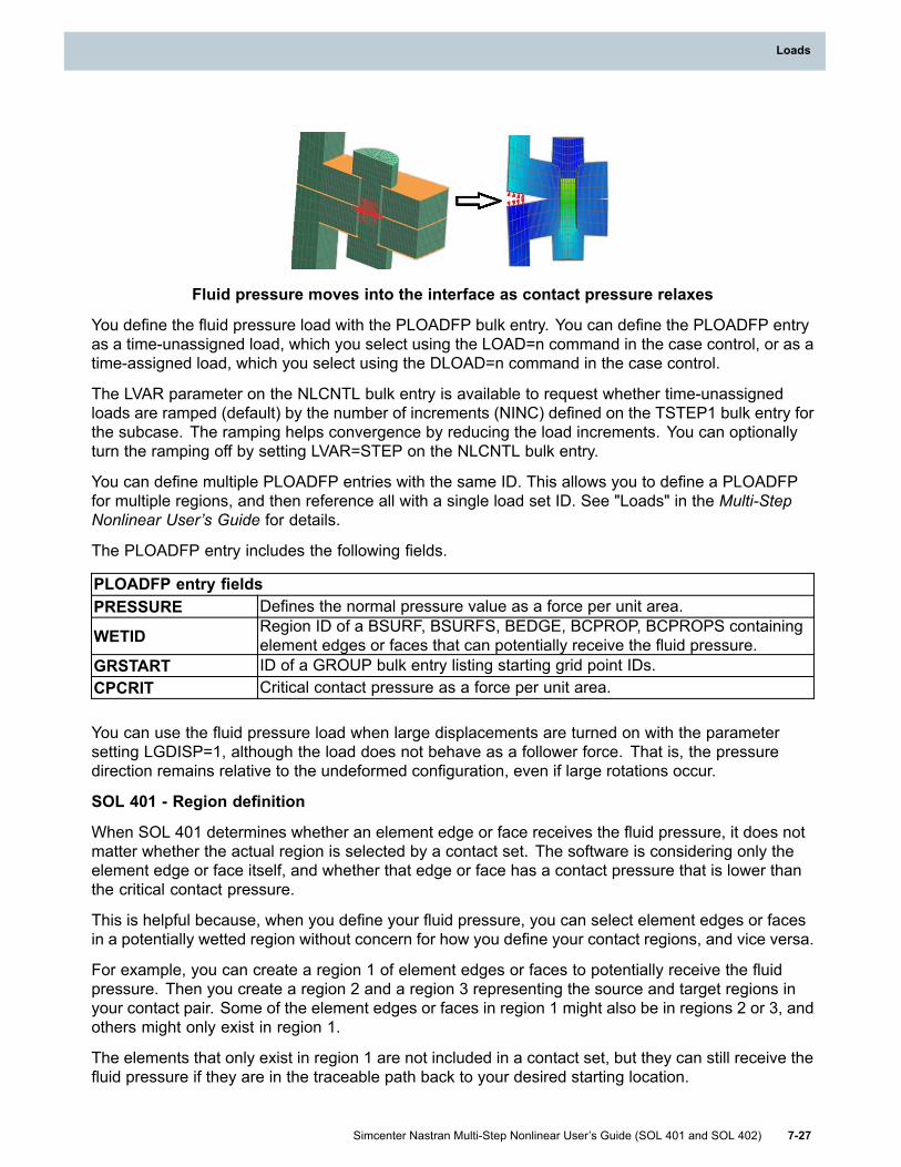
Loads
Fluid pressure moves into the interface as contact pressure relaxes
You define the fluid pressure load with the PLOADFP bulk entry. You can define the PLOADFP entryas a time-unassigned load, which you select using the LOAD=n command in the case control, or as atime-assigned load, which you select using the DLOAD=n command in the case control.
The LVAR parameter on the NLCNTL bulk entry is available to request whether time-unassignedloads are ramped (default) by the number of increments (NINC) defined on the TSTEP1 bulk entry forthe subcase. The ramping helps convergence by reducing the load increments. You can optionallyturn the ramping off by setting LVAR=STEP on the NLCNTL bulk entry.
You can define multiple PLOADFP entries with the same ID. This allows you to define a PLOADFPfor multiple regions, and then reference all with a single load set ID. See "Loads" in the Multi-StepNonlinear User’s Guide for details.
The PLOADFP entry includes the following fields.
PLOADFP entry fieldsPRESSURE Defines the normal pressure value as a force per unit area.
WETID Region ID of a BSURF, BSURFS, BEDGE, BCPROP, BCPROPS containingelement edges or faces that can potentially receive the fluid pressure.
GRSTART ID of a GROUP bulk entry listing starting grid point IDs.CPCRIT Critical contact pressure as a force per unit area.
You can use the fluid pressure load when large displacements are turned on with the parametersetting LGDISP=1, although the load does not behave as a follower force. That is, the pressuredirection remains relative to the undeformed configuration, even if large rotations occur.
SOL 401 - Region definition
When SOL 401 determines whether an element edge or face receives the fluid pressure, it does notmatter whether the actual region is selected by a contact set. The software is considering only theelement edge or face itself, and whether that edge or face has a contact pressure that is lower thanthe critical contact pressure.
This is helpful because, when you define your fluid pressure, you can select element edges or facesin a potentially wetted region without concern for how you define your contact regions, and vice versa.
For example, you can create a region 1 of element edges or faces to potentially receive the fluidpressure. Then you create a region 2 and a region 3 representing the source and target regions inyour contact pair. Some of the element edges or faces in region 1 might also be in regions 2 or 3, andothers might only exist in region 1.
The elements that only exist in region 1 are not included in a contact set, but they can still receive thefluid pressure if they are in the traceable path back to your desired starting location.
Simcenter Nastran Multi-Step Nonlinear User’s Guide (SOL 401 and SOL 402) 7-27
Loads

Chapter 7: Loads
The elements that exist in region 1 and in regions 2 or 3 are included in a contact set. They willreceive the fluid pressure only if their contact pressure is lower than the critical contact pressure,and they also must be in the traceable path.
The following summarizes the 2D and 3D regions you can reference with the WETID field.
Bulk entries to define contact regionsBSURF Defines a region on shell element faces.BCPROP (SOL 402only) Defines a region on shell element faces by property ID.
BSURFS Defines a region on 3D solid element faces.BCPROPS (SOL 402only) Defines a region on 3D solid element faces by property ID.
BEDGE Defines a region on 2D axisymmetric, chocking, plane strain and plane stresselement edges.
SOL 402 - Region definition
If the element regions you reference with the PLOADFP entry are also included in contact regions,SOL 402 requires that the contact definition should be defined with only a single contact pair on asingle BCTSET bulk entry.
For example, in the image below, represents the fluid pressure regions referenced by thePLOADFP, represents an incorrect contact definition in which two contact pairs are defined(four contact regions), and represents the correct contact definition in which one contact pair isdefined (two contact regions).
The following summarizes the 2D and 3D regions you can reference with the WETID field.
Bulk entries to define contact regionsBSURF Defines a region on shell element faces.BCPROP Defines a region on shell element faces by property ID.BSURFS Defines a region on 3-D solid element faces.BCPROPS Defines a region on 3-D solid element faces by property ID.
BEDGE Defines a region on 2-D axisymmetric, chocking, plane strain and planestress element edges.
Fluid pressure path
The fluid pressure path depends on the starting grid points you select in the GRSTART field.
7-28 Simcenter Nastran Multi-Step Nonlinear User’s Guide (SOL 401 and SOL 402)
Chapter 7: Loads

Loads
• The software uses only corner grid points for the starting locations and ignores any midsidegrid points you select in the GRSTART field.
• If you have not selected starting grid points in the GRSTART field, the software determinesstarting grids automatically using the grid points on the free boundaries of your region. Thefollowing two figures demonstrate the default start boundary for 2D and 3D regions.
2D region default starting boundary
3D region default start boundarySOL 401 - Fluid pressure updatesFor SOL 401, the parameter FPPUPDT is available on the NLCNTL bulk entry to control when thesoftware updates the fluid pressure load as a result of the changing contact status. By default,FPPUPDT=0, and the fluid pressure application is updated only at the beginning of every time stepusing the final contact status from the previous time step.
• FPPUPDT=0 (default)
The fluid pressure application is updated only at the beginning of every time step using the finalcontact status from the previous time step. For the first time step in a solution when there is noprevious contact status, the software does not apply fluid pressure to any elements, includingelements that are not in a contact region.
You will need to include enough time steps for the coupled contact and fluid pressure to becomeestablished and achieve a steady state. You should avoid a single time step solution. A warningmessage will be printed in the .f06 file if you define only a single time step in the first subcasethat includes fluid pressures.
In addition, you can define a preload subcase before the subcase in which your fluid penetratingpressures are applied to allow the contact conditions to become established. For this option,your contact regions must be either initially interferring, or you are including bolt preloads in thepreload subcase to push the contact regions together.
• FPPUPDT=1
The fluid pressure is updated for every solution iteration that occurs in a single time step. Thischoice will keep the fluid pressure current with the changing contact status. Defining FPPUPDT=1is more computational, and it can cause contact convergence issues if the fluid pressure andthe contact conditions are strongly coupled.
Fluid pressure output
Simcenter Nastran Multi-Step Nonlinear User’s Guide (SOL 401 and SOL 402) 7-29
Loads

Chapter 7: Loads
The existing OPRESS case control command has been updated with the FPP describer to requestthe fluid pressure output for the 2D and 3D regions referenced by the PLOADFP entry. You candisplay the OPRESS output in a post processor to visualize the edges or faces that receive and donot receive the fluid pressure for each time step.
The figure below illustrates the fluid pressure output on a contact region. The red faces receive thepressure and the blue faces do not.
You can also view the contact pressure results on the elements that are included in both contact andfluid pressure. Note that when using FPPUPDT=0, the software uses the contact status from theprevious time step to update the fluid pressure. As a result, when comparing fluid pressure applicationwith the contact pressure, you will need to look at the contact pressure from the previous time step.
OPRESS command pressure output
7.10 Initial stress-strain (SOL 401)Defining an initial stress or strain conditionThe option to define an initial stress or strain condition is available on all elements in SOL 401except for beam elements, shell elements, plane strain elements, generalized plane strain elements,solid composite elements, and rigid elements.
An unbalanced initial stress-strain results in deformation when applied to an unconstrained bodywith the possibility of residual stress.
Note that the definition of a Simcenter Nastran unbalanced initial stress-strain references theunconstrained body, although, an initial stress-strain can be applied to constrained or unconstrainedmodels.
A balanced initial stress-strain results in a self-equilibrating stress state and no deformations. SeeBalanced initial stress-strain section below.
You define the initial stress or strain with the INITS case control command, which selects the INITSbulk entry. The INITS case control command must be defined globally, above the subcases. Itis reapplied in every static subcase.
The first row on the INITS bulk entry includes the following fields.
• The TYPE field defines the data type: TYPE=STRESS or TYPE=STRAIN
• The CSYS field selects the coordinate system for the stress or strain components. The default isthe basic coordinate system. CSYS = -1 can also be defined to select the material system.
• The LOC field defines the location:
7-30 Simcenter Nastran Multi-Step Nonlinear User’s Guide (SOL 401 and SOL 402)
Chapter 7: Loads

Loads
LOC= GRID: Specifies that data is defined at grid points.
LOC= NOE: Specifies that data is defined on an element at grid locations. This can includecorner and/or midside grid locations.
You define the stress or strain data on the consecutive rows on the INITS entry. The softwareassumes the data is either engineering stress or engineering strain. The format of these rowsdepends on the data location defined in the LOC field, and the element type.
Format for the 3D solid elements CTETRA, CHEXA, CPENTA and CPYRAM:Stress at grid points (TYPE=STRESS, LOC=GRID):
GRID ID Sxx Syy Szz Sxy Syz Szx....
Strain data at grid points (TYPE=STRAIN, LOC=GRID):GRID ID Exx Eyy Ezz Exy Eyz Ezx
...
Stress data at the element corners (TYPE=STRESS, LOC=NOE):ElemID GRIDID Sxx Syy Szz Sxy Syz Szx
...
Strain data at the element corners (TYPE= STRAIN, LOC=NOE):ElemID GRIDID Exx Eyy Ezz Exy Eyz Ezx
...
For the plane stress elements CPLSTS3, CPLSTS4, CPLSTS6, CPLSTS8, the software uses bothin-plane and out-of-plane initial strain values. Although, only in-plane initial stress values are used.For example, the following formats should be used when the plane stress elements are defined onthe XY plane, and the basic coordinate system (default) is used. For elements defined on the XZplane, Sxx, Szz, Szx or Exx, Eyy, Ezz, Ezx would be defined.
Stress data at grid points (TYPE=STRESS, LOC=GRID):GRID ID Sxx Syy Sxy
...
Strain data at grid points (TYPE=STRAIN, LOC=GRID):GRID ID Exx Eyy Ezz Exy
...
Stress data at the element corners (TYPE=STRESS, LOC=NOE):ElemID GRIDID Sxx Syy Sxy
...
Strain data at the element corners (TYPE= STRAIN, LOC=NOE):ElemID GRIDID Exx Eyy Ezz Exy
...
For the axisymmetric elements CQUADX4, CQUADX8, CTRAX3, CTRAX6, in-plane (radial andaxial) and out-of-plane (theta) initial stress or strain values are used by the software. For example,the following formats should be used when the axisymmetric elements are defined on the XY plane,and the basic coordinate system (default) is used. For elements defined on the XZ plane, Sxx,Szz, Szx or Exx, Ezz, Ezx should be defined.
Stress data at grid points (TYPE=STRESS, LOC=GRID):GRID ID Sxx Syy Szz Sxy
Simcenter Nastran Multi-Step Nonlinear User’s Guide (SOL 401 and SOL 402) 7-31
Loads

Chapter 7: Loads
...
Strain data at grid points (TYPE= STRAIN, LOC=GRID):GRID ID Exx Eyy Ezz Exy
...
Stress data at the element corners (TYPE=STRESS, LOC=NOE):ElemID GRIDID Sxx Syy Szz Sxy
...
Strain data at the element corners (TYPE= STRAIN, LOC=NOE):ElemID GRIDID Exx Eyy Ezz Exy
...
For the plane stress and axisymmetric elements, if you select a coordinate system other than thebasic system in the CSYS field on the INITS entry, the software first transforms the data into the basicsystem, and then uses the components consistent with the formats described above.
An option to output the initial strains using the OSTNINI case control command is available. You canrequest the output at either the grid or corner Gauss locations on elements. The OSTNINI commandmust be defined globally, and the output occurs once at the beginning of the solution. The strains areoutput in the basic coordinate system.
Balanced initial stress-strain
A method is available that you can use to balance an unbalanced initial stress-strain. The methodremoves the unbalanced part by removing the strains that produce a deformation. For example,because approximate methods are used to measure residual stress, the application of the residualstress in your finite element analysis as an initial condition may not result in a state of completeequilibrium, and instead may result in both residual stress and deformation.
After you use the balancing method, your initial stress-strain will produce a self-equilibrating stressstate and no deformations.
The method requires that a part of your unbalanced initial stress-strain is actually balanced.
The balancing method requires that you first run a static offset-solution to obtain the total strain outputas a result of your unbalanced initial stress-strain with the model unconstrained. You only apply theunbalanced initial stress-strain in the offset solution. No temperature loads, mechanical loads, orenforced displacements are applied for this step.
Because there is no thermal strain {εth}, the total strain output {ε} from the offset-solution is computedas:
{ε} = {εe} + {εin} - {ε0}
where,
{ε} = total strains you can request with the STRAIN case control command,
{εe} = elastic strains you can request with the ELSTRN case control command,
{εin}= inelastic strains you can request with the PLSTRN or CRSTRN case control commands,
{ε0} = initial strains you can request with the OSTNINI case control command.
The part of the unbalanced initial stress-strain {ε0} that yields a stress is included in the elastic strain{εe} and possibly the inelastic strain {εin} if you have included any nonlinear materials. After removing
7-32 Simcenter Nastran Multi-Step Nonlinear User’s Guide (SOL 401 and SOL 402)
Chapter 7: Loads

Loads
{εe} and {εin} from the unbalanced initial stress-strain {ε0}, the total strain {ε} output from the offsetsolution includes only the part of the initial stress-strain that causes deformation.
You will use the total strain {ε} output from the offset-solution as an offset strain {εoff} in theconsecutive solution.
The total strain output is requested with the STRAIN=ALL case control command. If your modelcontains multiple components, each with a unique balanced initial strain, you can run an offset-solutionfor each component separately. The offset strains can be used in a consecutive assembly solution.
Note that, regardless of whether your initial stress-strain is applied to all locations on a component oronly to a portion, the offset strains are the total strains at all locations on that component.
To allow the static offset-solution to complete with the unconstrained condition, a matrix stabilizationoption is available. Setting the parameter MSTAB to 1 on the NLCNTL bulk entry will turn on theoption. In addition, the MSFAC parameter is available to define a scale factor for matrix stabilization.Specifically, when you define MSTAB=1, the software scales the diagonal terms by the factor(1+MSFAC).
Balanced solution
Once your offset strains are computed, you can run the consecutive balanced solution that includesyour initial stress-strain {ε0}, your offset strain {εoff}, and any other loads (temperature loads,mechanical loads, enforced displacements).
You can optionally run a consecutive balanced solution as unconstrained with only your initialstress-strain {ε0} and your offset strain {εoff} to verify that the strain offsets have removed alldeformation, leaving only the stress state. You can use the matrix stabilization option (MSTAB=1) inthe verification solution if you choose to keep your model unconstrained for this step. Finally, youcan apply initial stress-strain {ε0} and your offset strain {εoff} in a balanced component or assemblysolution that includes any load types and constraints.
During the balanced solution, the offset strains are included in the internal force calculation tocompensate for the deformations caused by your initial stress-strain. See Balanced stress-straincomputation for details.
Defining a balanced initial stress or strain condition
The INITS(OFFSET) case control command and INITSO bulk entry are available to input the offsetstrain. Multiple INITSO bulk entries can be combined with the existing INITADD bulk entry.
You define the initial stress-strain with the INITS case control command, which selects the INITS bulkentry. You can also define multiple INITS bulk entries, each with a unique ID, and then combine themusing the INITADD bulk entry. The INITADD entry is selected with the ID on the INITS case control.The INITS case control command must be defined globally, above the subcases. It is reapplied inevery static subcase.
The software does not need to associate a balanced initial stress-strain definition with an offset straindefinition in the balanced solution. As a result, the SID defined on the INITS(OFFSET) command thatselects your offset strains, and the SID defined on the INIT command that selects your unbalancedinitial stress-strain do not need to match.
Multiple initial stress-strain at the same location
You can define multiple unbalanced and balanced initial stress-strain at the same location. They canalso be defined using different coordinate systems. The software first converts all stress definitions to
Simcenter Nastran Multi-Step Nonlinear User’s Guide (SOL 401 and SOL 402) 7-33
Loads

Chapter 7: Loads
strain, then it transforms all strain into the basic coordinate system, and finally it adds the strainsdefined at common locations.
Balanced stress-strain computation
The reference (modeled) configuration of a component with balanced initial stress/strain includesinitial strains. Therefore, under the deformation field that results from combined initial strains andservice loads, the total strains measured from the reference configuration is given by:
{ε} = f({u}) + {εoff}
where,
f({u}) = [B]{u}
with [B] being the strain displacement matrix for small strain formulation.
The total strains are decomposed as:
{ε} = {εe} + {εth} + {εin} - {ε0}
where,
{ε} = total strains that you can request with the STRAIN case control command,
{εe} = elastic strains you can request with the ELSTRN case control command,
{εth} = thermal strains you can request with the THSTRN case control command,
{εin} = inelastic strains you can request with the PLSTRN case control command,
{ε0} = initial strains you can request with the OSTNINI case control command.
The elastic strains are obtained as,
{εe} = {ε} - {εth} - {εin} + {ε0}
In terms of balanced strain offsets, and assuming small strain formulation, the elastic strains aregiven by
{εe} = [B]{u} - {εth} - {εin} + ({ε0} + {εoff})
For components in the model without initial strains, {ε0} = {0} and {εoff} = {0}. For the components withunbalanced initial strains, {εoff} = {0}.
Note that if you request the total strain output {ε} for the balanced solution with the STRAIN casecontrol command, the software will add the offset strain back to the total as if it were never removedfor the solution. As a result, the total strain computation when a balanced initial stress-strain isdefined is the same as when an unbalanced initial stress-strain is defined.
Converting an initial stress to an initial strain
If you define an initial stress {σ0}, the software converts this to a corresponding initial strain {ε0} byusing the elasticity matrix {D0} at the reference temperature Tref.
{ε0} = {D0}-1 {σ0}
Additional information:
• Initial stress and strain can be defined on a subset of the model. The software assumes a valueof 0.0 at the locations where data is undefined. An exception is when data is undefined at amid-side grid point, and data is defined at both or either related corners. In this case, the softwareinterpolates a value for that mid-side grid point.
7-34 Simcenter Nastran Multi-Step Nonlinear User’s Guide (SOL 401 and SOL 402)
Chapter 7: Loads

Loads
• The option to apply an initial stress or strain condition before applying other loads in an initialsubcase is available to help convergence. The first subcase should have Tend=0.0 on theTSTEP1 entry and no load set selected. The number of increments can optionally be definedwith NINC on the TSTEP1 entry to increment the initial stress or strain. When NINC=1 (default),the initial stress or strain is applied in a single step. When NINC>1, the initial stress or strain isramped. A service load cannot be defined when ramping initial stress or strain with NINC>1.
• The software converts an initial stress to an initial strain using the elastic modulus defined onthe MATi entries. If you define MATTi bulk entries to define the elastic modulus as temperaturedependent, the software uses the initial temperatures selected by the TEMPERATURE(INIT)case control command to evaluate the temperature-dependent elastic modulus. Data on theMATS1 bulk entry, if defined, is not used to convert stress to strain.
• You can define multiple INITS bulk entries, each with a unique ID, and then combine them usingthe INITADD bulk entry. The INITADD entry is selected with the ID on the INITS case control. TheINITS entries selected by the INITADD entry must be all TYPE=STRESS or all TYPE=STRAIN.As a result, you cannot mix initial stress and initial strain definitions in the same input file.
• If you define data on the same grid or element corner location, a fatal error occurs.
7.11 Distributed force to a surface or edge (SOL 401)You can request that the software use forces and moments that you define at a single point toautomatically compute and apply a traction to a surface or edge region. The software computedtraction has a specific form and is described in the Traction computation details section.
You use the FORCDST bulk entry to define the point location, an optional point location offset, theforces and moments at the point, and to select the element or edge regions for the traction location.The element and edge regions that receive the traction are defined as follows.
• You use the BSURF entry to create face regions on the shell elements CTRIA3, CTRIA6,CTRIAR, CQUAD4, CQUAD8, and CQUADR.
• You use the BSURFS entry to create face regions on the solid elements CHEXA, CPENTA,CPYRAM, and CTETRA.
• You use the BEDGE entry to create edge regions on the following elements:
Axisymmetric elements CTRAX3, CQUADX4, CTRAX6, CQUADX8.
Plane stress elements CPLSTS3, CPLSTS4, CPLSTS6, CPLSTS8.
Chocking elements CCHOCK3, CCHOCK4, CCHOCK6, CCHOCK8
You have the option on the FORCDST bulk entry to define the single point location for your forcesand moments at a grid point, at a coordinate system origin, or at the centroid of the surface or edgeregion you have selected to receive the traction. The software automatically computes the centroidlocation of the surface or edge region.
For a time-unassigned load, you reference the SID of the FORCDST bulk entry and any othermechanical loads with the LOAD=n case control command either in a subcase or above the subcases(globally).
Simcenter Nastran Multi-Step Nonlinear User’s Guide (SOL 401 and SOL 402) 7-35
Loads
Chapter 7: Loads
For example,
...SUBCASE 5LOAD = 150BEGIN BULK...$ TIME-UNASSIGNED LOADS FOR SUBCASE 5FORCDST,150,10,,CNTRD,,,,,++,1.0,23.4,428.6,84,2,49.7,7846.4,5876.5...RFORCE,150,5,,-6.4,0.0,0.0,1.0,2...
For a time-assigned load, you must select the FORCDST bulk entry with the EXCITEID on theTLOAD3 bulk entry. The TLOAD3 entry includes six TID fields that you can use to independentlyscale the three force and the three moment components with time by referencing a unique TABLEDientry for each. You can also reference the same TABLEDi entry for any or all TID fields to define thesame load variations. The FORCDST entry is the only load you can select with the TLOAD3 entry.All other time-assigned mechanical loads are selected by the EXCITEID of the TLOAD1 bulk entry,which scales all referenced loads consistently with time. You can combine TLOAD1 and TLOAD3entries into a single load set with the DLOAD bulk entry.
For example,
...SUBCASE 5$DLOAD CASE CONTROL SELECTS THE DLOAD BULK ENTRYDLOAD = 250BEGIN BULK...$DLOAD BULK ENTRY COMBINES TLOAD3 (ID=302) and TLOAD1 (ID=305)DLOAD,250,1.,1.,302,1.,305...$TIME-ASSIGNED FORCDST, EXCITEID=125, TIME FUNCTION FOR EACH COMPONENTTLOAD3,302,125,,,,,,,++,,401,402,403,501,502,503...FORCDST,125,10,,CNTRD,,,,,++,1.0,23.4,428.6,84.2,49.7,78.4,56.5...$SOLID ELEMENT REGION TO RECEIVE TRACTIONBSURFS,10,,,,8,10,15,40,++,12,15,20,45,16,20,25,50,++,24,35,40,65,28,40,45,70,++,32,45,50,75,40,60,65,90...$TIME FUNCTIONS FOR EACH COMPONENT DEFINED ON FORCDSTTABLED2,401,0.,++,0.,0.,1.,100.,2.,0.,ENDTTABLED2,402,0.,++,0.,0.,1.,120.,2.,0.,ENDTTABLED2,403,0.,++,0.,0.,1.,140.,2.,0.,ENDTTABLED2,501,0.,++,0.,0.,1.,80.,2.,0.,ENDT
7-36 Simcenter Nastran Multi-Step Nonlinear User’s Guide (SOL 401 and SOL 402)
Chapter 7: Loads

Loads
TABLED2,502,0.,++,0.,0.,1.,90.,2.,0.,ENDTTABLED2,503,0.,++,0.,0.,1.,100.,2.,0.,ENDT...$TIME-ASSIGNED RFORCE, EXCITEID=150, TIME FUNCTION TID=13TLOAD1,305,125,13$TIME FUNCTION 13 USED FOR FORCE LOADTABLED2 13 0. + 0. 0. 1. 100. 2. 0. ENDTRFORCE,150,5,,-6.4,0.0,0.0,1.0,2...
The FORCDST bulk entry includes the optional point location offset. This offset is simply added to thepoint location defined on the FORCDST bulk entry. The software does not scale the point location orthe offset with time. The TABLEDi entry you reference from a TID field only scales the associated forceor moment value. As a result, the location of the forces and moments remain constant for a solution.
The software always computes the traction based on the undeformed configuration. It does not takeinto account large displacements or rotations when recomputing the traction at a time step.
Traction computation details
Figure 7-1 shows an example element patch to illustrate the procedure. You define the FORCDSTbulk entry to apply the forces and moments at point D or optionally at the centroid (C), and to selectthe element patch where the software computes and applies the traction.
Figure 7-1. Element patch and load locations
The software computes the centroid (C) of the element patch. If you defined your forces and momentsat D, the software transfers them to an equivalent system at C using a rigid link transformation,
where is the vector from C to D.
If you define your forces and moments at the centroid location (C), the software skips the step oftransfering the forces and moments from location D to C.
Simcenter Nastran Multi-Step Nonlinear User’s Guide (SOL 401 and SOL 402) 7-37
Loads

Chapter 7: Loads
A local coordinate system is computed on the patch using the eigenvectors of the inertia matrix. Theeigenvector associated with the largest eigenvalue is the x3 direction. This direction is perpendicularto a flat surface or approximately perpendicular to a curved surface. The next two eigenvectorsbecome the x1 and x2 directions, respectively.
The software will compute the following traction on the patch:
where are the coordinates of the patch grid points relative to the local patch coordinates
.
The assumption is that the computed traction must satisfy the following requirements.
• The resultant force computed using the forces from all grid points on the patch must equal theforce resultant at C.
• The resultant moment computed using the moments from all grid points on the patch mustequal the moment resultant at C.
Rearranging the terms in the traction gives:
The traction vector is written as a superposition of six traction loads:
The six traction load cases are as follows (per unit surface area or per unit length).
is a uniformly distributed load of unit intensity in the direction.
is a linearly varying load in the direction.
is a linearly varying load in the direction.
is a uniformly distributed load of unit intensity in the direction.
is a uniformly distributed load of unit intensity in the direction.
is a linearly varying load in the and directions.
The grid point force vector due to surface traction is given by integrating over the entire patch:
Substituting into the equation above gives:
7-38 Simcenter Nastran Multi-Step Nonlinear User’s Guide (SOL 401 and SOL 402)
Chapter 7: Loads

Loads
Each term can be written as a grid point force vector:
The grid point force vector for the patch is a linear combination of the grid point force vectors fromeach load case:
The original total load requirements are applied here. This results in a 6x6 system of equations thatthe software uses to solve for C1, C2, …C6.
• The resultant force of all grid point forces on the patch must be the same as the forces at point C.The resultant force is computed by:
• The resultant moment of all grid point forces on the patch must be the same as the moments atpoint C. The resultant moment is computed by:
where is the grid point position with respect to the centroid (C).
There are now six equations to solve for the six unknowns C1, C2, ….,C6.
These equations are resolved into scalar equations.
The software uses the following 6x6 matrix to compute C1, C2, ….,C6.
Simcenter Nastran Multi-Step Nonlinear User’s Guide (SOL 401 and SOL 402) 7-39
Loads

Chapter 7: Loads
For time-unassigned loads, this matrix is used once to compute C1, C2, ….,C6.
For time-assigned loads, this matrix is reused to recompute C1, C2, ….,C6 at each time step. Theright-hand side is updated with the updated force and moment values at each time step.
7.12 SOL 401 - RFORCE and RFORCE1 scalingWhen you define the RFORCE or RFORCE1 bulk entries for SOL 401 as either time-assigned,
or as time-unassigned and ramped, the software uses time to scale the angular velocity and
acceleration , which it uses to compute the inertia force.
You define the time variation either using a time-assigned load referenced by the DLOAD=ncase control command, or by a time-unassigned load referenced by the LOAD=n case controlcommand, which is ramped. You request this ramping using the LVAR parameter on the NLCNTLbulk entry.
The angular velocity is computed as:
where,
is the rotation vector defined on the RFORCEi entry,
and A is the scale factor of the angular velocity in revolutions per unit time defined on the RFORCEientry.
The associated force is computed as:
where,
m is the mass computed at each grid point Gi,
and ri and ra are position vectors (not related to the rotation vector). See the remarks on the RFORCEientries for a definition of the position vectors.
The RFVAR parameter is available on the NLCNTL bulk entry to change how the software interpolatesthe time variation.
• When RFVAR=OMEGA (default), the software interpolates the time variation using .
7-40 Simcenter Nastran Multi-Step Nonlinear User’s Guide (SOL 401 and SOL 402)
Chapter 7: Loads

Loads
As a result, if you define a linear time variation, the angular velocity will vary linearly. Becauseis squared in the force computation, the force will not vary linearly.
This default behavior is the same as the previous release. You must define the RFVAR=FORCEsetting described below to see a change in the interpolation.
• When RFVAR=FORCE, the software interpolates the time variation using . The softwarethen takes the square root of the interpolated value before applying it to the angular velocity.
As a result, if a linear time variation is defined, the force will vary linearly, but will not.
Note that the RFVAR parameter setting changes the interpolation only for angular velocity, and not forangular acceleration. Because the angular acceleration is not squared in the force computation, itvaries linearly with the force.
For example, suppose you define solution times from 0.0 to 1.0 second in 5 increments, at time=0.0,f(t)=0.0, and at time=1.0, f(t)=2.0.
Assume A=1.0, m is an identity matrix,
and , where is a unit vector.
The following table and plot shows the resulting values of and for this simplified input scenario.
RFVAR=OMEGA RFVAR=FORCE
Time
0.0 0.0 0.0 0.0 0.00.2 0.4 0.16 0.894427 0.80.4 0.8 0.64 1.264911 1.60.6 1.2 1.44 1.5491933 2.40.8 1.6 2.56 1.788854 3.21.0 2.0 4.0 2.0 4.0
Simcenter Nastran Multi-Step Nonlinear User’s Guide (SOL 401 and SOL 402) 7-41
Loads

Chapter 7: Loads
7-42 Simcenter Nastran Multi-Step Nonlinear User’s Guide (SOL 401 and SOL 402)
Chapter 7: Loads

Chapter 8: Contact conditions (SOL 401)
8.1 Contact OverviewSOL 401 supports surface-surface and edge-edge contact. The algorithm supports largedeformations and finite sliding between contact pairs. For large deformation problems (LGDISP>-1),the contact stiffness and contact forces are rotated with the geometry consistent with other elementformulation in SOL 401. In addition, the SOL 401 contact algorithm updates the geometry and pairingwhen there is finite sliding between the contacting surfaces.
Contact is modeled using a contact set, contact regions, contact segments and contact pairs.
The table below lists the case control commands and bulk entries used to define contact.
Contact definition summary
Case control commands:BCSET Selects a contact set.BCRESULTS Selects contact results to output.
Bulk entries related to edge or surface definition:BSURF Defines contact region on shell elements.BCPROP Defines contact region on shell elements by property ID.BSURFS Defines contact region on 3-D solid elements.BCPROPS Defines contact region on 3-D solid elements by property ID.
BEDGE Defines contact region on 2-D axisymmetric, chocking, plane strainand plane stress elements.
BCRPARA Defines parameters for contact region.
Bulk entries related to contact set definition:BCTSET Defines the contact sets.BCTADD Defines a union of contact sets.BCTPARM Defines parameters for contact sets.
8.2 Contact Subcase ControlThe BCSET case control command selects the contact conditions defined in the bulk data. TheBCSET command can be defined in any static, dynamic, or bolt preload subcase type. For example,you can remove or add contact regions and pairs, and change contact settings including parameters,from one static or preload subcase to the next.
The modal, cyclic, and Fourier subcase types which are sequentially dependent (default) use the finalstiffness from a previous static or bolt preload subcase. The final stiffness from a static, dynamic, orpreload subcase includes the contact stiffness.
Simcenter Nastran Multi-Step Nonlinear User’s Guide (SOL 401 and SOL 402) 8-1

Chapter 8: Contact conditions (SOL 401)
Contact conditions are supported with the restart capability.
Note that if a subcase is sequentially dependent and it includes a new contact set, any contacttractions from a previous subcase will be used as an initial condition for the current subcase. Theprevious tractions define the initial condition for the newly formed contact elements.
8.3 Contact DefinitionEdge Contact Regions
An edge contact region is a collection of axisymmetric, chocking, plane strain, and plane stresselement free edges in a section of the model where you expect contact to occur. You create edgeregions with the BEDGE bulk entry.
• To define a contact edge using the BEDGE entry, you enter the element ID along with the cornerGRID IDs. You can define the edges on the BEDGE entry in any order.
Edge-to-edge contact can be defined on the edges of the following elements:
• Axisymmetric elements CTRAX3, CQUADX4, CTRAX6, CQUADX8.
• Chocking elements CCHOCK3, CCHOCK4, CCHOCK6, CCHOCK8.
• Plane stress elements CPLSTS3, CPLSTS4, CPLSTS6, CPLSTS8.
• Plane strain elements CPLSTN3, CPLSTN4, CPLSTN6, CPLSTN8.
The axisymmetric, chocking, plane stress, and plane strain elements can be defined in either the XZplane or in the XY plane. Edge-to-edge contact is supported in either orientation. The generalizedplane strain element is not supported by glue or contact regions.
Surface Contact Regions
A surface contact region is a collection of element free faces in a section of the model where youexpect contact to occur. These regions can be created using the shell elements (BSURF andBCPROP) and using solid element free faces (BSURFS and BCPROPS).
• The BSURF entry is defined by its own unique ID and is a list or range of shell element IDs toinclude in the region.
• The BCPROP entry is defined by its own unique ID and is a list of shell element property IDs.Shell elements which use any of these listed property IDs will be included in the region.
• The BSURFS entry is defined by its own unique ID and is a list of solid element IDs each followedby 3 grid points defining which face of the 3-D element to include in the contact region.
• The BCPROPS entry is defined by its own unique ID and is a list of solid element property IDs.The free faces of the solid elements selected with a property ID are automatically determinedby the software.
Surface-to-surface contact can be defined on the faces of the following elements.
• 3-D Solid elements CHEXA, CPENTA, CPYRAM, and CTETRA.
8-2 Simcenter Nastran Multi-Step Nonlinear User’s Guide (SOL 401 and SOL 402)
Chapter 8: Contact conditions (SOL 401)
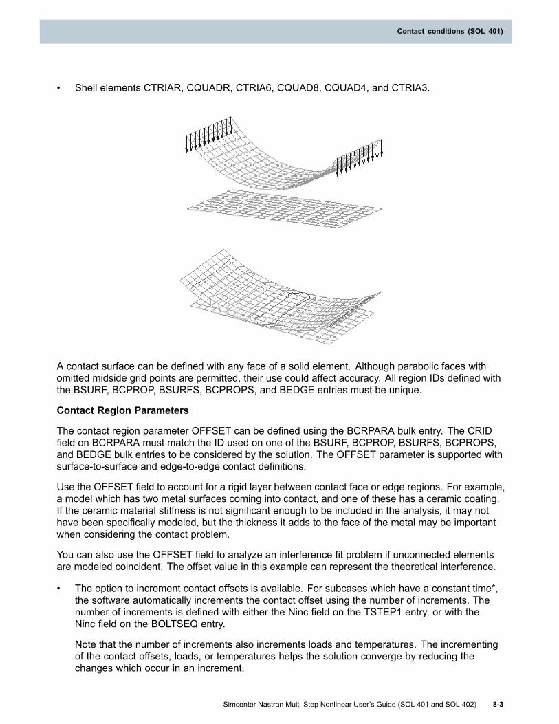
Contact conditions (SOL 401)
• Shell elements CTRIAR, CQUADR, CTRIA6, CQUAD8, CQUAD4, and CTRIA3.
A contact surface can be defined with any face of a solid element. Although parabolic faces withomitted midside grid points are permitted, their use could affect accuracy. All region IDs defined withthe BSURF, BCPROP, BSURFS, BCPROPS, and BEDGE entries must be unique.
Contact Region Parameters
The contact region parameter OFFSET can be defined using the BCRPARA bulk entry. The CRIDfield on BCRPARA must match the ID used on one of the BSURF, BCPROP, BSURFS, BCPROPS,and BEDGE bulk entries to be considered by the solution. The OFFSET parameter is supported withsurface-to-surface and edge-to-edge contact definitions.
Use the OFFSET field to account for a rigid layer between contact face or edge regions. For example,a model which has two metal surfaces coming into contact, and one of these has a ceramic coating.If the ceramic material stiffness is not significant enough to be included in the analysis, it may nothave been specifically modeled, but the thickness it adds to the face of the metal may be importantwhen considering the contact problem.
You can also use the OFFSET field to analyze an interference fit problem if unconnected elementsare modeled coincident. The offset value in this example can represent the theoretical interference.
• The option to increment contact offsets is available. For subcases which have a constant time*,the software automatically increments the contact offset using the number of increments. Thenumber of increments is defined with either the Ninc field on the TSTEP1 entry, or with theNinc field on the BOLTSEQ entry.
Note that the number of increments also increments loads and temperatures. The incrementingof the contact offsets, loads, or temperatures helps the solution converge by reducing thechanges which occur in an increment.
Simcenter Nastran Multi-Step Nonlinear User’s Guide (SOL 401 and SOL 402) 8-3
Contact conditions (SOL 401)

Chapter 8: Contact conditions (SOL 401)
*A constant time subcase has a TSTEP1 bulk entry defined with either Tend=0.0, or a Tend whichis the same as the start time for that subcase.
• When a sequentially dependent subcase is defined with SEQDEP=YES, the final contact offsetfrom a previous subcase, if it exists, is included at the start of the current subcase. The goal is tohelp convergence when contact offsets change from one subcase to the next. In this case, theoffset for the current subcase is calculated as:
OFFSET = OC*LF+OP*(1 - LF)
Where:OC = Contact offset for the current subcase,OP = Contact offset from a previous subcase,and LF = Load factor incremented in Ninc steps. The initial value is 1/Ninc and the final valueis 1.0.
• General recommendations for offset definitions:
- A separate subcase is recommended to resolve the contact offset.
- When bolt preloads and contact offsets are defined together, be aware that both can result inaxial bolt strain. If you do not want the contact offset to result in an additional bolt strain, thecontact offset should be modeled with a slight gap.
• You can optionally change the contact offset definition from one subcase to the next by selectingunique contact sets in each subcase which reference different BCRPARA bulk entries.
Contact Pairs
A contact pair combines two contact regions, source and target, in which contact will be analyzedduring the solution. Each contact pair can have its own unique friction value (if desired) and searchdistance.
The BCTSET bulk entry is used to define both edge-to-edge and surface-to-surface contact pairs.The CID field will need to match the value of ‘n' on the BCSET case control entry for the solutionto recognize this contact definition.
The SIDi and TIDi fields on the BCTSET bulk entry are used to define source and target regionsrespectively for a pair. As many pairs as desired can be included on a single BCTSET entry. Eachpair can have a unique friction value (optional), a minimum search distance, and a maximum searchdistance. You can define the optional Coefficient of Friction field (FRICi) for each contact pair. Whencontact is detected, the solver uses this value to calculate any tangential contact forces.
The regions you select with SID and TID depend on the type of contact:
• For edge-to-edge contact pairs, SID and TID are contact regions defined with the BEDGE entry.
• For surface-to-surface contact pairs, SID and TID are contact regions defined with the BCPROP,BCPROPS, BSURF, and BSURFS entries.
The minimum and maximum search distance fields (MINDi and MAXDi) define a range in which thesolver can initially determine if the distance between element edges or faces in a particular pair arewithin the threshold for creating contact elements. These values are used to determine where contactelements are created. The minimum distance can be negative if there is an interference conditionmodeled as overlapping regions.
8-4 Simcenter Nastran Multi-Step Nonlinear User’s Guide (SOL 401 and SOL 402)
Chapter 8: Contact conditions (SOL 401)

Contact conditions (SOL 401)
The contact condition can update when large sliding occurs when large displacement effects areturned off (PARAM,LGDISP,-1) or on (PARAM,LGDISP,1).
Combining Contact Sets – BCTADD
You can optionally define multiple BCTSET/BCTPARM bulk entry sets, each set with uniquecontact set IDs (CSID), and then combine them with a single BCTADD bulk entry. The multipleBCTSET/BCTPARM bulk entry sets are created to adjust certain contact parameters locally. Contactparameters can also be adjusted globally with a BCTPARM bulk entry having the same CSID asthe BCSET case control command.
The following example demonstrates the inputs.
CASE CONTROL$CSID on the BCSET case control matches CSID on BCTADDBCSET = 108...BULK DATA$Local Contact Set definitionsBCTSET 1 1 2 0.0 1.0BCTSET 2 3 4 0.15 0.0 0.15 6 0.15 0.0 0.1...$Local Contact ParametersBCTPARM 1 PENN 10 PENT 1BCTPARM 2 PENN 1.0 PENT 0.1...$Local Contact Sets are combined with BCTADDBCTADD 108 1 2...$Global Contact ParametersBCTPARM 108 MAXS 30 NCHG 0.02
See the section “Contact Control Parameters - BCTPARM” for more information on contactparameters.
Contact with Composite Solid Faces
Defining contact regions and pairs on composite solid faces which are perpendicular to the stackdirection (edge faces) may produce poor stress continuity. If the contact definition is between edgefaces belonging to different PCOMPS definitions, and if the number of plies on each PCOMPSdefinition is small and the same, and the ply thicknesses are similar, the stress continuity should befairly smooth. This also applies to the results requested with the BCRESULTS case control command.
Additional Recommendations
When defining contact regions and pairs on geometry which are not tangent continuous, creatingsingle contact regions which cross corner transitions can result in non-uniform stress results aroundthe corners. It is recommended to break these areas into multiple regions and pairs as shown below.
Simcenter Nastran Multi-Step Nonlinear User’s Guide (SOL 401 and SOL 402) 8-5
Contact conditions (SOL 401)

Chapter 8: Contact conditions (SOL 401)
When defining contact regions and pairs, it is recommended to not include the same element face inmultiple regions. In “A” below, an element is repeated in regions 2 and 3. In “B”, the same elementonly exists in region 2. “B” is recommended. Repeating element faces multiple times in the same ordifferent regions can significantly increase memory requirements and degrade performance.
8.4 Contact Control ParametersThe contact control parameters on the BCTPARM bulk entry can help you adjust the contactalgorithm when you are having problems getting a solution to converge and complete, or when thecontact results are not as expected. For many solutions, the default settings are appropriate, andthe BCTPARM entry is not required.
You can optionally define multiple BCTSET/BCTPARM bulk entry sets, each set with uniquecontact set IDs (CSID), and then combine them with a single BCTADD bulk entry. The multipleBCTSET/BCTPARM bulk entry sets are created to adjust certain contact parameters locally. Contactparameters can also be adjusted globally with a BCTPARM bulk entry having the same CSID asthe BCSET case control command.
8-6 Simcenter Nastran Multi-Step Nonlinear User’s Guide (SOL 401 and SOL 402)
Chapter 8: Contact conditions (SOL 401)

Contact conditions (SOL 401)
Global and local contact parameters have the following definition and rules:
• Global Contact Parameters
The BCTPARM bulk entry, which uses the same CSID entered on the BCSET case controlcommand, defines global parameters.
Any of the parameters on the BCTPARM bulk entry can be defined globally. A parameter’s defaultvalue is used if it is not defined globally or locally.
• Local Contact Parameters
The BCTPARM bulk entries associated to individual BCTSET bulk entries, which are thencombined with a BCTADD bulk entry, define local parameters.
See the Parameters for SOL 401 listed on the BCTPARM bulk entry in the Quick Reference Guide.
8.5 Contact kinematicsConsider the contact element between the points S and T in the figure below. S and T are theparametric locations of a contact element on the source and target faces respectively.
S1, S2, S3, S4,...Sj are the grid points defining one solid element face which is included in thesource region.
T1, T2, T3, T4,...Tj are the grid points defining one solid element face which is include in the targetregion.
Figure 8-1. Contact Source and Target Example
The global system of equations including contact at a given iteration i is:
Equation 8-1.
Where:
Simcenter Nastran Multi-Step Nonlinear User’s Guide (SOL 401 and SOL 402) 8-7
Contact conditions (SOL 401)

Chapter 8: Contact conditions (SOL 401)
is the assembled contact stiffness,
is the assembled nodal contact forces,
NCE is the total number of contact elements created,
Kc is the contact stiffness from a single contact element,
and Fc are the contact forces from a single contact element,
The total traction for a contact element c at an iteration i can be split into normal and tangentialcomponents as:
Equation 8-2.
where is the normal vector, and the tangential vector is .
Together , t1, and t2 form an ortho-normal basis.
Normal contact conditions
The normal contact conditions can be expressed as:
Equation 8-3.
Equation 8-4.
Equation 8-5.
Equation 8-3 imposes the condition that the penetration of the hitting surface into the target surface
can’t be greater than zero. Thus, surfaces can’t interpenetrate. The contact pressure, , is definedas the negative of the normal component of the surface traction.
Equation 8-4 states that the contact pressure can’t be less than zero or tensile. Or normal tractionsbetween surfaces can’t be tensile.
Equation 8-5 imposes the condition that:
and
SOL401 uses a penalty method to enforce the contact constraints with the ability to augment thetractions (Augmented Lagrangian formulation) to keep the penetrations to within a specified tolerance(PTOL).
8-8 Simcenter Nastran Multi-Step Nonlinear User’s Guide (SOL 401 and SOL 402)
Chapter 8: Contact conditions (SOL 401)

Contact conditions (SOL 401)
The pure penalty method can be activated by setting MAXS=1 on BCTPARM bulk data entry. Purepenalty method is computationally in-expensive and in most cases produces acceptable solution.However, since there is no check on penetration control this method can sometime cause largepenetrations in the model that could go undetected.
Augmented Lagrangian formulation is the default. With this method, first a converged solution isobtained with a penalty method. If the convergence criteria have not been achieved, the tractionsare augmented and another series of iterations is performed until convergence is achieved. Thetractions could be augmented several times until either the desired level of penetration tolerance(PTOL) is achieved when the convergence criteria is based on penetrations or alternately thetractions between two augmentations are converged to a value below CTOL for convergence criteriabased on augmented tractions. MAXS (default=20) parameter specifies the maximum number ofaugmentations that are performed for every time step. If the augmentation convergence is notachieved within MAXS number of iterations the solution will proceed to the next step if the usualglobal convergence criteria have been satisfied.
The normal traction is:
Equation 8-6.
is the normal traction from previous augmentation.
Note that =0 for the pure penalty method.
εn is the normal penalty stiffness (unit=force/length),
is the contact element normal gap evaluated at iteration i,
K is the augmentation loop ID.
The relative displacement at a contact element location for iteration i is computed as:
Equation 8-7.
The contact element normal gap at iteration i is calculated as
Equation 8-8.
Simcenter Nastran Multi-Step Nonlinear User’s Guide (SOL 401 and SOL 402) 8-9
Contact conditions (SOL 401)

Chapter 8: Contact conditions (SOL 401)
Equation 8-9.
Nj = Standard Source Face shape functions evaluated at the contact point
N'k = Standard Target Face shape functions evaluated at the contact point
Ns = Number of nodes on source face
Nt = Number of nodes on target face
Xs=X0s + UsXt=X0t + UTX0s = Undeformed coordinates of the nodes on the source face
X0t = Undeformed coordinates of the nodes on the target face
Us = Nodal displacements on the source face
Ut = Nodal displacements on the target face.
Note that a positive value of indicates an overlap and a negative value indicates a separationbetween the source and target faces at the contact element location.
Consequently a contact element is considered CLOSED if > 0 and OPEN if < 0.
The tangential traction is
Equation 8-10.
where,
λnt is the tangential traction from previous step.
εt is the tangential penalty factor (unit=force/length),
is the relative displacement increment in the tangential direction since last time step where j= 1, 2.
The relative displacement increment in the tangential direction is calculated as:
Equation 8-11.
where,
8-10 Simcenter Nastran Multi-Step Nonlinear User’s Guide (SOL 401 and SOL 402)
Chapter 8: Contact conditions (SOL 401)

Contact conditions (SOL 401)
Equation 8-12.(ΔUs) = Nodal displacement increment since last time step on the source side DOF.
(ΔUt)= Nodal displacement increment since last time step on the target side DOF.
A contact element can have the following states:
Inactive when < 0.
Active when > 0.
Coulomb FrictionIf friction is present (μ > 0 where μ is the coulomb friction coefficient), an active contact element canhave either sticking or sliding state.
Similar to the normal contact conditions, the frictional contact conditions can be expressed as:
Equation 8-13.
Equation 8-14.
Equation 8-15.
Equation 8-16.
Equation 8-13 imposes the constraint that the magnitude of the in-plane friction traction, , cannotexceed the coefficient of friction μ, times the normal contact traction. When the magnitude of frictionforce reaches its maximum allowable value, the function Φ will be equal to zero.
Equation 8-14 relates the relative tangential displacement increment between the source and
the target surface, , to the magnitude of the relative slip increment, , which must be anon-negative quantity.
Equation 8-16 implies that if ≥ 0 (there is slipping between the surfaces), then Φ= 0, and if
= 0 (the surfaces are sticking), then Φ ≤ 0.
Simcenter Nastran Multi-Step Nonlinear User’s Guide (SOL 401 and SOL 402) 8-11
Contact conditions (SOL 401)

Chapter 8: Contact conditions (SOL 401)
Therefore, for Coulomb friction:
• The maximum possible tangential traction equals the coefficient of friction times the normaltraction force.
• Contacting surfaces will "stick" if the tangential traction is less than the coefficient of friction timesthe normal traction force.
• Contacting surfaces will "slide" in the direction of the tangential traction if the tangential tractionequals the coefficient of friction times the normal traction force.
Figure 8-2. Classical Coulomb Friction Model (FRICMOD=0)
Assume
A contact element state is Sticking if
Equation 8-17.
and Sliding if
Equation 8-18.
Bilinear Coulomb Friction (FRICMOD=1)
8-12 Simcenter Nastran Multi-Step Nonlinear User’s Guide (SOL 401 and SOL 402)
Chapter 8: Contact conditions (SOL 401)

Contact conditions (SOL 401)
Figure 8-3. Bi-Linear Coulomb Friction ModelBy default, SOL401 uses a bi-linear coulomb model specified by FRICMOD=1 on BCTPARM. Thismodel converges better than the classical model (FRICMOD=0) by providing a more distinct stick slipzone. Here, the tangential penalty factor εT is adaptively computed based on the current contactpressure, coefficient of friction and a critical slip value Scrit provided by the user. The default for Scritis set at 0.5% of the characteristic element length in the pair. A larger value of Scrit helps witheasier convergence but leads to more sliding, while a smaller value represents the exact coulombbehavior more closely but also leads to slower convergence rates. The tangential stiffness is updatedevery iteration using:
Equation 8-19.The incremental tangential relative displacement can be expressed as a sum of elastic and plasticparts.
Equation 8-20.or
Equation 8-21.
where is the elastic slip at the end of previous step.
The predictor slip is
Equation 8-22.
Simcenter Nastran Multi-Step Nonlinear User’s Guide (SOL 401 and SOL 402) 8-13
Contact conditions (SOL 401)

Chapter 8: Contact conditions (SOL 401)
The trial tangential traction is evaluated from the predicted slip as:
Equation 8-23.
This predicted slip is elastic as long as the magnitude of the tangential traction is less than the
critical stress (i.e.) .
If the magnitude of the tangential traction exceeds the critical stress then slip must be taken intoaccount.
The magnitude of the plastic slip in this instance is given by where isthe magnitude of the predicted slip.
The incremental slip is computed as:
Equation 8-24.
When the slip output is requested, the total slip is computed as the algebraic sum of the incrementalslip (elastic and plastic) over time. The incremental slip is the difference in total slip between twooutput intervals.
Additional friction models:
FRICMOD=2: Friction is computed using the following product which optionally depends on time,velocity or temperature:
μ(t,T,v)= FPARA1 * CFVE(v) * CFTE(T) * CFNF(t)
FPARA1, CFNF, CFTE, and CFVE are all parameters defined on the BCTPARM entry. FRICi onthe BCTSET entry is ignored.
FPARA1 defines a constant friction value, and CFNF, CFTE, CFVE are integer inputs which referenceTABLEDi entries defining friction as a function of time, temperature, and velocity, respectively. If anyof CFNF, CFTE, or CFVE are undefined, their contribution is ignored.
FRICMOD=3: Two different friction coefficients are used depending on the sliding velocity.
This friction model uses the parameters VCRIT, FPARA1, and FPARA2 on the BCTPARM entry.FRICi on the BCTSET entry is ignored.
VCRIT defines the critical sliding velocity, FPARA1 (1 in the image below) defines the frictioncoefficient when the sliding velocity < VCRIT, and FPARA2 (2 in the image below) defines the frictioncoefficient when the sliding velocity > VCRIT.
8-14 Simcenter Nastran Multi-Step Nonlinear User’s Guide (SOL 401 and SOL 402)
Chapter 8: Contact conditions (SOL 401)
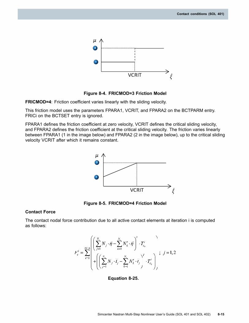
Contact conditions (SOL 401)
Figure 8-4. FRICMOD=3 Friction Model
FRICMOD=4: Friction coefficient varies linearly with the sliding velocity.
This friction model uses the parameters FPARA1, VCRIT, and FPARA2 on the BCTPARM entry.FRICi on the BCTSET entry is ignored.
FPARA1 defines the friction coefficient at zero velocity, VCRIT defines the critical sliding velocity,and FPARA2 defines the friction coefficient at the critical sliding velocity. The friction varies linearlybetween FPARA1 (1 in the image below) and FPARA2 (2 in the image below), up to the critical slidingvelocity VCRIT after which it remains constant.
Figure 8-5. FRICMOD=4 Friction Model
Contact Force
The contact nodal force contribution due to all active contact elements at iteration i is computedas follows:
Equation 8-25.
Simcenter Nastran Multi-Step Nonlinear User’s Guide (SOL 401 and SOL 402) 8-15
Contact conditions (SOL 401)

Chapter 8: Contact conditions (SOL 401)
Equation 8-26.
Contact Stiffness
From the normal component of traction we have:
Equation 8-27.
For a sticking contact element with friction,
Equation 8-28.
For a slipping contact element,
Equation 8-29.
The contact stiffness contribution after ignoring the variation of friction coefficient with pressureand sliding velocity is:
Equation 8-30.
8-16 Simcenter Nastran Multi-Step Nonlinear User’s Guide (SOL 401 and SOL 402)
Chapter 8: Contact conditions (SOL 401)

Contact conditions (SOL 401)
Equation 8-31.
Equation 8-32.
The global contact stiffness is obtained by summing the stiffness contribution from all active contactelements:
Equations 8-31 and 8-32 include non-symmetric stiffness terms. Using an un-symmetric solverwill significantly increase the memory requirements. The software automatically activates theun-symmetric solver if the coefficient of friction is greater than FSYMTOL. The parameter FSYMTOL(specified on NLCNTL) has a default value of 0.2.
Contact Iterations
The contact problem is solved by a dual loop algorithm with the augmentation loop serving as theouter loop and the regular NR iterations constituting the inner loop. In addition to the global criteriato determine the inner iterations convergence, contact algorithm also checks for contact forceconvergence. The inner loop is said to be converged if the change in contact force between twoconsecutive iterations is < RCTOL. After the convergence of the inner loop (i.e.) NR iterations,the tractions are augmented if needed and another round of inner iterations is done until either ofthe following 2 criteria is met:
1. CNTCONV=1. In this case the outer loop convergence criteria are based on penetrationtolerance. The augmentations are performed until the max penetration in each contact pair isbelow the tolerance PTOL.
2. CNTCONV=2. In this case the outer loop convergence criteria are based on contact tractionconvergence ratio CTOL. The contact tractions are augmented until the augmented force ratioFRAT change in the tractions between two consecutive augmentation loops is converged to avalue smaller than CTOL.
Simcenter Nastran Multi-Step Nonlinear User’s Guide (SOL 401 and SOL 402) 8-17
Contact conditions (SOL 401)

Chapter 8: Contact conditions (SOL 401)
Contact Algorithm FlowchartSteps 1 through 4 occur for each time step (n+1).
1. Loop over contact augmentations (K=1 to MAXS).
a. Initialize λkn .
b. Compute stiffness K and Kc.
2. Do Newton-Raphson iterations (i=1 to MAXITER).
a. Compute internal forces and where is the force contribution from contact.
b. Compute Residual
c. Solve (see equations 8-30 through 8-32 ).
d. Check for the solution convergence based on global criteria and RCTOL. The global solutionconvergence criteria are defined by the CONV parameter on the NLCNTL bulk entry.
A. If the solution convergence criteria are satisfied, go to step 3.
B. If the solution convergence criteria is not satisfied:
i. If (i < MAXITER) then do more iterations, go to 2a or if stiffness update is required,go to step 1b.
ii. If (i = MAXITER) then convergence is not achieved and end problem. GO TO step 4.
3. Check outer loop convergence for contact based on either PTOL or CTOL.
a. If the contact outer loop is converged, end the problem. Go to step 4.
b. If the outer loop is not converged, increment the outer loop counter, augment the tractions,and go to step 1b.
4. End Problem.
8.6 Contact Penalty FactorsThe normal penalty stiffness εn and the tangential penalty stiffness εT are computed for each contactelement as follows:
εn = Ac * E * PENN
εT = Ac * E * PENT
8-18 Simcenter Nastran Multi-Step Nonlinear User’s Guide (SOL 401 and SOL 402)
Chapter 8: Contact conditions (SOL 401)

Contact conditions (SOL 401)
PENN and PENT are the normal and tangential penalty factors respectively. Ac is the area associatedwith the contact element and E is the modulus of the softer region in the contact pair.
The normal penalty is computed by the contact algorithm or can be input by the user. The automaticpenalty factor calculation estimates geometry characteristics using element edge lengths in thevicinity of the contact regions. The solver computes a characteristic length Lc for each contact pairand estimates the normal penalty factor PENN as PENN = 1 / Lc. The default value of PENT isan order of magnitude smaller than the PENN.
When the option to adaptively compute the tangential stiffness is selected, the tangential penaltyfactor is adjusted based on current contact pressure, coefficient of friction and critical slip parameter.
PENT = μ * Tn / ScritThe penalty factors influence the rate of convergence, and to a lesser extent, the accuracy of thecontact solution. The automatic penalty factor calculation works well for most instances, but manualadjustments may be necessary, particularly if a contact problem fails to converge. When the problemfails to converge or takes a lot of iterations to converge, reducing the default value of PENN by anorder or two of magnitude will generally help with convergence.
A large value of PENN will make the system of equations ill-stabled leading to convergence problems.They could also produce spotty contact pressure results. In addition, a small value of PENN maycause excessive penetrations which will require more traction augmentations. So the right choice ofpenalty factors is the key to getting good quality contact stress results in a reasonable number ofiterations.
The software provides an alternate way (PENTYP=2) to input PENN and PENT as spring rate perarea. That is, Force/(Length x Area). The contact element stiffness in this case is calculated as:
εn = Ac * PENN
εT = Ac * PENT
The spring rate input is a more explicit way of entering contact stiffness since it is not dependenton the modulus.
The auto-calculated values for PENN and PENT can be scaled using the AUTOSCAL and TANSCLparameters respectively. The range for AUTOSCAL is usually 0.01 - 1.0 with the default being 1.0.The default works well for bulk deformation dominant problems. For bending dominant or finite slidingproblems, a smaller range 0.01 - 0.1 is recommended.
8.7 Contact Sliding and Geometry UpdateThe contact element locations on the element faces or edges are updated based on the value of theDISP, GUPDATE, and GUPTOL parameters.
The DISP parameter on the BCTPARM bulk entry is available to select the sliding formulation. Thesoftware only considers your GUPDATE and GUPTOL parameter settings when you use the DISP= 0 option.
DISP Behavior
0 (Default)
Contact pairing is automatically detemined by the software based on theamount of relative sliding in the pair. The software considers your GUPDATEand GUPTOL parameter settings (described below). If you have not explicitlydefined the GUPDATE and GUPTOL parameters, the default values are used.
Simcenter Nastran Multi-Step Nonlinear User’s Guide (SOL 401 and SOL 402) 8-19
Contact conditions (SOL 401)
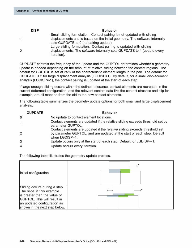
Chapter 8: Contact conditions (SOL 401)
DISP Behavior
1Small sliding formulation. Contact pairing is not updated with slidingdisplacements and is based on the initial geometry. The software internallysets GUPDATE to 0 (no pairing update).
2Large sliding formulation. Contact pairing is updated with slidingdisplacements. The software internally sets GUPDATE to 4 (update everyiteration).
GUPDATE controls the frequency of the update and the GUPTOL determines whether a geometryupdate is needed depending on the amount of relative sliding between the contact regions. Thedefault for GUPTOL is set at 25% of the characteristic element length in the pair. The default forGUDPATE is 2 for large displacement analysis (LGDISP=1). By default, for a small displacementanalysis (LGDISP=-1), the contact pairing is updated at the start of each step.
If large enough sliding occurs within the defined tolerance, contact elements are recreated in thecurrent deformed configuration, and the relevant contact data like the contact stresses and slip forexample, are all mapped from the old to the new contact elements.
The following table summarizes the geometry update options for both small and large displacementanalysis.
GUPDATE Behavior0 No update to contact element locations.
1 Contact elements are updated if the relative sliding exceeds threshold set byparameter GUPTOL.
2Contact elements are updated if the relative sliding exceeds threshold setby parameter GUPTOL, and are updated at the start of each step. Defaultwhen LGDISP=1.
3 Update occurs only at the start of each step. Default for LGDISP=-1.4 Update occurs every iteration.
The following table illustrates the geometry update process.
Initial configuration
Sliding occurs during a step.The slide in this exampleis greater than the value ofGUPTOL. This will result inan updated configuration asshown in the next step below.
8-20 Simcenter Nastran Multi-Step Nonlinear User’s Guide (SOL 401 and SOL 402)
Chapter 8: Contact conditions (SOL 401)

Contact conditions (SOL 401)
Contact configuration isupdated after the magnitudeof the slide exceeds the valuedefined on the parameterGUPTOL.
8.8 Contact and rigid body motionMany static problems depend on contact to provide the boundary conditions necessary for a stableproblem. With these problem types, the stiffness matrix can be singular when the contact constraintsare inactive. You can use the following options to avoid singularities.
• Open and closed contact stiffness
The contact algorithm automatically adds a small stiffness at the start of the solution which isoften enough to prevent rigid body motion. In some instances, the default initial stiffness may beinsufficient to prevent large displacements. In such cases, you can redefine an initial stiffnesswith the OPNSTF parameter on the BCTPARM bulk entry.
The OPNSTF parameter works in conjunction with the OPNTOL parameter which specifies thegap up to which OPNSTF will be enforced. The default for OPNSTF is 1.0E-6 * the closedstiffness, and the OPNTOL default is the characteristic length of the contact pair. If the gap closesin the subsequent iteration, the closed stiffness will be applied to the contact element.
The following graph demonstrates the open and closed contact stiffness change. The horizontalaxis represents the contact gap, and the vertical axis represents the contact element stiffness.
go = open stiffness gap defined by the OPNTOL parameter.
gc = closed stiffness gap defined by the GAPTOL parameter.
Kopen = open stiffness is used when the gap is smaller than OPNTOL, but greater than GAPTOL.
Kclosed = closed stiffness is used when the gap is smaller that GAPTOL.
• Stiffness stabilization
Simcenter Nastran Multi-Step Nonlinear User’s Guide (SOL 401 and SOL 402) 8-21
Contact conditions (SOL 401)

Chapter 8: Contact conditions (SOL 401)
To allow a solution to complete with an unconstrained condition, a matrix stabilization option isavailable. Setting the parameter MSTAB to 1 on the NLCNTL bulk entry will turn on the option.
In addition, the MSFAC parameter is available to define a scale factor for matrix stabilization.Specifically, when you define MSTAB=1, the software scales the diagonal terms by the factor(1+MSFAC).
• Displacement scaling
Limiting the maximum incremental displacement per iteration is useful when a load is applied to abody that is not initially in contact. A model can be unstable even when stiffness stabilization oropen stiffness is used resulting in excessive initial displacement. Setting the limiting displacementto about the element size in this case would scale down the potentially huge displacement inthe first iteration so that the results remain close to the converged solution. The displacementscaling feature can be thought of as a form of line search. This option is on by default and can beturned off by setting DISCAL=0 on the BCTPARM bulk entry. You can also adjust the limitingfactor with the DISTOL parameter on the BCTPARM bulk entry.
• Contact Stabilization Damping
In order to stabilize rigid body motion caused before contact is engaged, a damping force can beapplied to keep the parts from flying off. The stabilization normal damping force is computedas follows:
where is the normal damping coefficient, is the pseudo relative velocity of the contactsurfaces in the normal direction.
The normal damping coefficient is internally calculated by the solver. You can either scale oroverwrite the auto computed damping coefficient by entering the value as a function of contactpressure per velocity.
The damping coefficient is calculated based on the contact stiffness, contact gap and currentsolution time with respect to the subcase end time.
where CTDAMPN is the scale factor with a default value of 1.0,
Krep is a fraction of the closed contact stiffness,
,
Gapfac = 0 when gap > opntol or gap < 0.
The default value for OPNTOL is equal to 1.0 (times average element length).
,
where Curtim is the current solution time and Send is the subcase end time.
Thus by default the effects of the damping are ramped down to zero by the end of the firstsubcase.
8-22 Simcenter Nastran Multi-Step Nonlinear User’s Guide (SOL 401 and SOL 402)
Chapter 8: Contact conditions (SOL 401)

Contact conditions (SOL 401)
Also, once the contact is established the damping effects vanish.
When CTDAMP=1 or 2, the damping is applied to a contact pair only when the entire pair isopen. Even if one contact element in the pair is active, the stabilization stiffness is not applied.However, when CTDAMP=3, the stabilization stiffness is applied for any contact element that isopen with a gap smaller than OPNTOL.
Also, When CTDAMP > 1, the damping is not ramped down as a function of time and will beapplied always.
Similar to normal damping coefficient, tangential damping coefficient is also computed when thereis friction. The tangential damping coefficient is computed as:
CT = CTDAMPT * CN where CTDAMPT is the tangential scale factor with default = 0.001.
The tangential damping force is thus calculated as:
Where is the pseudo relative velocity in the tangential direction.
8.9 Contact Offsets, Gaps, and PenetrationsInitial Gaps and Penetrations
The treatment of initial gaps and penetrations is governed by the INIPENE and ADJUST parameterson the BCTPARM entry. The INIPENE parameter requests that the software reset a gap orpenetration. The ADJUST parameter requests that the software move the grid points when thereare gaps.
The adjustment is applied at the start of the solution based on the initial geometry. It is ideal for smalldisplacement analysis or press-fit assemblies.
If both INIPENE and ADJUST are defined, ADJUST is first applied, then INIPENE.
The INIPENE options are as follows.
• INIPENE = 0 (default): Contact is evaluated as the geometry is modeled.
• INIPENE = 1: Gaps are reset to a new initial condition.
• INIPENE = 2: Penetrations are reset to a new initial condition in which there is no interference.
• INIPENE = 3: Gaps and penetrations are both reset to a new initial condition in which there isno interference.
When you use the ADJUST parameter on the BCTPARM bulk entry, the software uses an adjustmenttolerance to move the source grid points on to the target faces when the absolute value of the initialseparation distance is below the adjustment tolerance. The adjustment tolerance is computed asADJUST * characteristic length.
• ADJUST = 0.0: Only the grid points that are initially overclosed are adjusted as long as theover-closure is below the characteristic length.
Simcenter Nastran Multi-Step Nonlinear User’s Guide (SOL 401 and SOL 402) 8-23
Contact conditions (SOL 401)

Chapter 8: Contact conditions (SOL 401)
• ADJUST > 0.0: The adjustment is applied to grid points that are initially open with a gap smallerthan the value of ADJUST * characteristic length.
Contact Surface Offsets
An offset distance can be specified for a contact region on the BCRPARA entry, and for a contact pairon the BCTPARM bulk entry. The OFFSET parameter on the BCTPARM bulk entry overwrites anoffset defined for a region on the BCRPARA entry.
For example, a model which has two metal surfaces coming into contact, and one of these has aceramic coating. If the ceramic material stiffness is not significant enough to be included in theanalysis, it may not have been specifically modeled, but the thickness it adds to the face of the metalmay be important when considering the contact problem.
You can also use the OFFSET field to analyze an interference fit problem if unconnected elementsare modeled coincident. The offset value in this example can represent the theoretical interference.
• A separate subcase is recommended to resolve the contact offset prior to the application ofservice loads.The offsets can be resolved incrementally based on the value of NINC parameteron the TSTEP1 bulk entry.
• When bolt preloads and contact offsets are defined together, be aware that both can result inaxial bolt strain. If you do not want the contact offset to result in an additional bolt strain, thecontact offset should be modeled with a slight gap.
• The option to increment contact offsets is available. For subcases which have a constant time*,the software automatically increments the contact offset using the number of increments. Thenumber of increments is defined with either the Ninc field on the TSTEP1 entry, or with theNinc field on the BOLTSEQ entry.
Note that the number of increments also increments loads and temperatures. The incrementingof the contact offsets, loads, or temperatures helps the solution converge by reducing thechanges which occur in an increment.
*A constant time subcase has a TSTEP1 bulk entry defined with either Tend=0.0, or a Tend whichis the same as the start time for that subcase.
• When a sequentially dependent subcase is defined with SEQDEP=YES, the final contact offsetfrom a previous subcase, if it exists, is included at the start of the current subcase. The goal is tohelp convergence when contact offsets change from one subcase to the next. In this case, theoffset for the current subcase is calculated as:
OFFSET = OC*LF+OP*(1 - LF)
Where:OC = Contact offset for the current subcase,OP = Contact offset from a previous subcase,and LF = Load factor incremented in Ninc steps. The initial value is 1/Ninc and the final valueis 1.0.
• You can optionally change the contact offset definition from one subcase to the next by selectingunique contact sets in each subcase which reference different BCRPARA / BCTPARM bulkentries.
8-24 Simcenter Nastran Multi-Step Nonlinear User’s Guide (SOL 401 and SOL 402)
Chapter 8: Contact conditions (SOL 401)

Contact conditions (SOL 401)
• For shell element regions, you can also use the SHLTHK and ZOFFSET parameters on theBCTPARM bulk entry as follows:
SHLTHK is the shell thickness offset flag. By default, the contact surface is assumed to be offsett/2 from the nodes defining a shell element. If the FE mesh represents the outer surface, set thisvalue to 1 so the thickness offset will be ignored.
ZOFFSET determines if the shell element z-offset is included in the contact solution. By default,shell z-offsets are included. ZOFFSET=1 will prevent them from being included.
• If you define both the OFFSET and INIPENE parameters, the software adds the offset after itevaluates any gaps or penetrations as a result of the INIPENE setting.
Ramping the Removal of Penetrations in a time assigned subcase
The TZPENE parameter on the BCTPARM bulk entry is available to ramp the removal of initialpenetrations for time assigned subcases. For example, if you have modeled contact surfacespenetrating to represent a press fit condition.
TZPENE: End time when initial penetrations will be eliminated.
TZPENE=0.0 (Default): The initial penetrations are eliminated in the first subcase.
For example, if a subcase start time is 5.0, end time is 10.0, and TZPENE=7.2, the initial penetrationswill be eliminated starting from the beginning of the subcase (5.0) until time=7.2. Ramping theremoval of initial penetrations can help convergence.
Ramping the Removal of Penetrations in a constant time subcase
The IPENRAMP parameter on the BCTPARM bulk entry is available to ramp the removal of initialpenetrations for a constant time subcase. For example, a preload subcase is a constant time subcase.
Interference Example
Consider the following example.
The red area represents a 3D solid mesh and the green area represents a 2D shell element mesh.Contact is defined between the shell mesh and the bottom of the solid mesh.
The gap (g) between the shell element face region (midplane where the grid points are modeled) andthe solid face region is 0.1.
The shell element thickness (t) is 0.4.
SOL 401 applies shell thickness first, then INIPENE settings, and finally offsets. For each of thefollowing cases, when ramping is requested with either the TZPENE or IPENRAMP parameters, thesoftware will ramp the initial penetration result shown.
1) The shell thickness is included, there are no INIPENE effects, and no offsets. The initial penetration= (t/2 - g)=(0.2 - 0.1) = 0.1.
Simcenter Nastran Multi-Step Nonlinear User’s Guide (SOL 401 and SOL 402) 8-25
Contact conditions (SOL 401)

Chapter 8: Contact conditions (SOL 401)
2) Same as 1 except INIPENE=3. The penetration of 0.1 would be reset to 0.0. The initial penetration= 0.0.
3) Same as 2 except an offset of 0.3 is defined on the solid contact region (BCRPARA bulk entry).The penetration of 0.1 would be reset to 0.0, but because the offset is applied last, the initialpenetration = offset = 0.3.
4) Same as 3 except GAPVAL=0.1 is now defined. The penetration of 0.1 would be reset to 0.0,then GAPVAL resets to an initial gap of 0.1, and finally, since the offset is applied last, the initialpenetration = (OFFSET-GAPVAL) = (0.3 - 0.1) = 0.2.
8.10 Contact Surface and Edge RefinementThe refinement of the source and target occurs by default. The contact search algorithm identifies foreach source segment a set of closest target segments that could potentially come into contact.
Each potential target segment is projected on to the source face or edge and a polygon clippingalgorithm computes an overlapping area. The overlapped area is divided into triangles creating a“refined” source face/edge [3]. Integration points are created on each triangle based on gaussquadrature rules and the value of the INTORD entry on the BCTPARM bulk entry.
The contact conditions are enforced at these integration points. The refinement process captures thecontact domain accurately and is an important piece in passing the constant stress patch test.
8-26 Simcenter Nastran Multi-Step Nonlinear User’s Guide (SOL 401 and SOL 402)
Chapter 8: Contact conditions (SOL 401)

Contact conditions (SOL 401)
The refinement feature can optionally be turned off by setting REFINE=0 on the BCTPARM entry.
8.11 Contact ConvergenceThe software prints all of the relevant information pertaining to each contact pair at the start of thesolution. Contact max penetration (PRATIO) and change in forces (RCTOL) are printed as part of theiteration summary. PRATIO is the ratio of max penetration in the current iteration for all pairs and thecorresponding penetration tolerance (PTOL) in that pair. In addition to the global convergence criteriabeing met, the PRATIO and RCTOL criteria should also be met for contact problems.
See Iteration related output data (SOL 401) for an example and description of the convergencedata in the .f06 file.
Convergence considerations
• A high value of RCTOL (>1.0) or a large percentage change in contact status in each iterationusually indicates any combination of the following.
o The penalty factor is high.
o The load is being applied too quickly.
o The time step is large.
To correct this situation, you can adjust AUTOSCAL to 0.1 or lower, or you can reduce theload and time steps.
• If the PRATIO values are consistency higher than 1.0 but RCTOL and other convergencenorms are decreasing, increasing the penalty factor by an order can help achieve penetrationconvergence.
• Most convergence issues can be attributed to either loss of contact or the penalty factors beingtoo high or low. If there is rigid body motion present, setting open stiffness or stiffness stabilizationwould help at the start of the analysis.
• If the displacements are constantly getting scaled, either the loading is excessive or the contacthas been lost. If there are initial gaps/penetrations in the geometry, setting INIPENE to ignorethese would help.
Simcenter Nastran Multi-Step Nonlinear User’s Guide (SOL 401 and SOL 402) 8-27
Contact conditions (SOL 401)
Chapter 8: Contact conditions (SOL 401)
• If there are excessive numbers of contact pairing updates in a step, then the load or time step istoo large.
• If contact is lost due to difficult geometry or sharp changes in the geometry, reducing the step sizeor geometry update tolerance (GUPTOL) can help.
• The contact algorithm monitors these variables for abrupt changes and triggers a bisection if thenumber of adverse changes within a step exceeds the value of CNTMDIV.
• Use FRICDLY to delay friction effects until after the first step can also alleviate convergenceproblems. With this option turned on, the frictional conditions are applied one time stepafter contact is established. This feature can be useful in many problems, since it delays thenonlinearity associated with friction until contact is established.
• If the convergence is slow or cannot be achieved for models with friction, using the un-symmetricsolver can improve the convergence rates.
8.12 Contact OutputContact results can be requested with the BCRESULTS case control command. Forces, tractions,separation distance, total and incremental slide or slip distance, and contact status can be output.
The SEPDIS describer requests the final separation distance for grids on both the source and targetregions. It is computed based on the current deformed configuration. For grids on the source region,the separation distance is a scalar quantity representing the source side normal distance to the target.For grids on the target region, the separation distance is a scalar quantity representing the target sidenormal distance to the source. During the solution, the separation distance is known at the elementintegration points, but is written to the grids when output. The result at each source and target gridis the value of separation distance at the closest contact element. If there are two or more contactelements equidistant from the grid, then the minimum value of separation distance is used at the gridsrather than the average, since the average gives unexpected results for coarse meshes.
In addition for SOL 401, the SEPDIS describer requests the total and incremental slide distance forgrids on both the source and target regions. The slide distance is reported in the basic coordinatesystem as the algebraic sum of the incremental slip (elastic and plastic) from each increment. Whena contact grid goes inactive, the total slide distance output resets to zero. The incremental slidedistance is the difference in the total slide distance between two output intervals.
When the contact status is requested with the STATUS describer on the BCRESULTS command,an integer value indicating the contact status is output on each grid point included in a contactsource or target region. The status values are:
0: No contact exists.
1:A sticking contact condition exist.
2: A sliding contact condition exist.
8-28 Simcenter Nastran Multi-Step Nonlinear User’s Guide (SOL 401 and SOL 402)
Chapter 8: Contact conditions (SOL 401)

Contact conditions (SOL 401)
8.13 References1. T.A. Laursen and J.C. Simo. "Algorithmic Symmetrization of Coulomb Frictional Problems Using
Augmented Lagrangians". Computers Methods in Applied Mechanics and Engineering. Vol. 108,No. 1& 2. 133-146. 1993.
2. P. Wriggers. “Computational Contact Mechanics”. Second Edition.
3. M. Puso, T. Laursen. “A Mortar Segment-to-Segment Frictional Contact Method for LargeDeformations”, Computer Methods in Applied Mechanics and Engineering, 2003.
Simcenter Nastran Multi-Step Nonlinear User’s Guide (SOL 401 and SOL 402) 8-29
Contact conditions (SOL 401)


Chapter 9: Contact conditions (SOL 402)
9.1 Contact overviewSOL 402 supports surface-surface and edge-edge contact. The algorithm supports largedeformations and finite sliding between contact pairs. For large deformation problems (LGDISP>-1),the contact stiffness and contact forces are rotated with the geometry consistent with other elementformulation in SOL 402. In addition, the SOL 402 contact algorithm updates the geometry and pairingwhen there is finite sliding between the contacting surfaces.
Contact is modeled using a contact set, contact regions, contact segments and contact pairs.
The table below lists the case control commands and bulk entries used to define contact.
Contact definition summary
Case control commands:BCSET Selects a contact set.BCRESULTS Selects contact results to output.
Bulk entries related to edge or surface definition:BSURF Defines contact region on shell elements.BCPROP Defines contact region on shell elements by property ID.BSURFS Defines contact region on 3-D solid elements.BCPROPS Defines contact region on 3-D solid elements by property ID.
BEDGE Defines contact region on 2-D axisymmetric, plane strain and planestress elements.
BCTPAR2 Defines parameters for contact region.
Bulk entries related to contact set definition:BCTSET Defines the contact sets.BCTADD Defines a union of contact sets.
9.2 Contact subcase controlThe BCSET case control command selects the contact conditions defined in the bulk data. TheBCSET command can be defined in any subcase type.
The modal, cyclic, and Fourier subcase types, which are sequentially dependent (default), use thefinal stiffness from a previous subcase. The final stiffness from a static or preload subcase includesthe contact stiffness.
Note that if a subcase is sequentially dependent and it includes a new contact set, any contacttractions from a previous subcase will be used as an initial condition for the current subcase. Theprevious tractions define the initial condition for the newly formed contact elements.
Simcenter Nastran Multi-Step Nonlinear User’s Guide (SOL 401 and SOL 402) 9-1

Chapter 9: Contact conditions (SOL 402)
9.3 Contact definition
Edge contact regions
An edge contact region is a collection of axisymmetric, chocking, plane strain, and plane stresselement free edges in a section of the model where you expect contact to occur. You create edgeregions with the BEDGE bulk entry.
• To define a contact edge using the BEDGE entry, you enter the element ID along with the cornerGRID IDs. You can define the edges on the BEDGE entry in any order.
Edge-to-edge contact can be defined on the edges of the following elements:
• Axisymmetric elements CTRAX3, CQUADX4, CTRAX6, CQUADX8.
• Plane stress elements CPLSTS3, CPLSTS4, CPLSTS6, CPLSTS8.
• Plane strain elements CPLSTN3, CPLSTN4, CPLSTN6, CPLSTN8.
The axisymmetric, plane stress, and plane strain elements can be defined in either the XZ plane or inthe XY plane. Edge-to-edge contact is supported in either orientation. The generalized plane strainelement is not supported by glue or contact regions.
Surface contact regions
A surface contact region is a collection of element free faces in a section of the model where youexpect contact to occur. These regions can be created using the shell elements (BSURF andBCPROP) and the solid element free faces (BSURFS and BCPROPS).
• The BSURF entry is defined by its own unique ID and is a list or range of shell element IDs toinclude in the region.
• The BCPROP entry is defined by its own unique ID and is a list of shell element property IDs.Shell elements that use any of the listed property IDs will be included in the region.
• The BSURFS entry is defined by its own unique ID and is a list of solid element IDs each followedby three grid points defining which face of the 3D element to include in the contact region.
• The BCPROPS entry is defined by its own unique ID and is a list of solid element property IDs.The software automatically determines the free faces of the solid elements selected with aproperty ID.
Surface-to-surface contact can be defined on the faces of the following elements.
• 3-D Solid elements CHEXA, CPENTA, CPYRAM, and CTETRA.
• Shell elements CTRIAR, CQUADR, CTRIA6, CQUAD8, CQUAD4, and CTRIA3.
9-2 Simcenter Nastran Multi-Step Nonlinear User’s Guide (SOL 401 and SOL 402)
Chapter 9: Contact conditions (SOL 402)
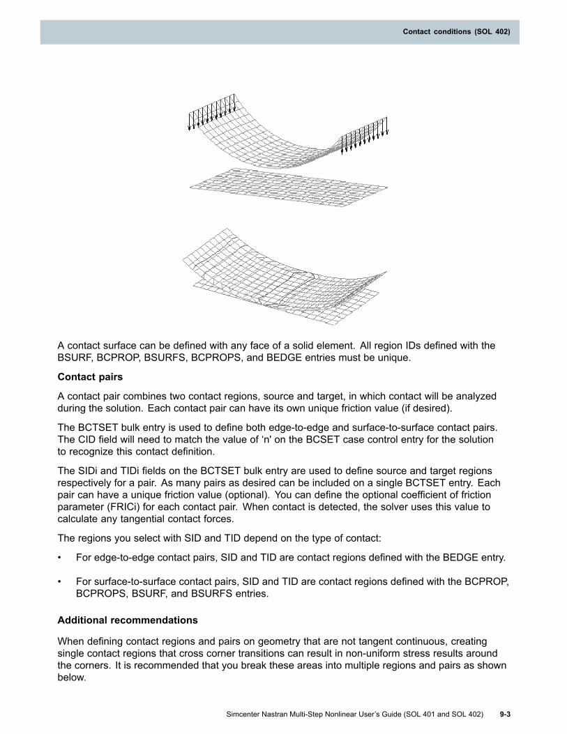
Contact conditions (SOL 402)
A contact surface can be defined with any face of a solid element. All region IDs defined with theBSURF, BCPROP, BSURFS, BCPROPS, and BEDGE entries must be unique.
Contact pairs
A contact pair combines two contact regions, source and target, in which contact will be analyzedduring the solution. Each contact pair can have its own unique friction value (if desired).
The BCTSET bulk entry is used to define both edge-to-edge and surface-to-surface contact pairs.The CID field will need to match the value of ‘n' on the BCSET case control entry for the solutionto recognize this contact definition.
The SIDi and TIDi fields on the BCTSET bulk entry are used to define source and target regionsrespectively for a pair. As many pairs as desired can be included on a single BCTSET entry. Eachpair can have a unique friction value (optional). You can define the optional coefficient of frictionparameter (FRICi) for each contact pair. When contact is detected, the solver uses this value tocalculate any tangential contact forces.
The regions you select with SID and TID depend on the type of contact:
• For edge-to-edge contact pairs, SID and TID are contact regions defined with the BEDGE entry.
• For surface-to-surface contact pairs, SID and TID are contact regions defined with the BCPROP,BCPROPS, BSURF, and BSURFS entries.
Additional recommendations
When defining contact regions and pairs on geometry that are not tangent continuous, creatingsingle contact regions that cross corner transitions can result in non-uniform stress results aroundthe corners. It is recommended that you break these areas into multiple regions and pairs as shownbelow.
Simcenter Nastran Multi-Step Nonlinear User’s Guide (SOL 401 and SOL 402) 9-3
Contact conditions (SOL 402)

Chapter 9: Contact conditions (SOL 402)
When defining contact regions and pairs, it is recommended that you do not include the same elementface in multiple regions. In “A” below, an element is repeated in regions 2 and 3. In “B”, the sameelement only exists in region 2. “B” is recommended. Repeating element faces multiple times in thesame or different regions can significantly increase memory requirements and degrade performance.
Note
The source contact regions (SIDi) that are initially defined as set of element faces orelements are converted in set of nodes by the solver. This should be taken into accountwhen splitting target regions as explained above.
9.4 Contact control parametersThe contact control parameters on the BCTPAR2 bulk entry can help you adjust the contact algorithmwhen you are having problems getting a solution to converge and complete, or when the contact
9-4 Simcenter Nastran Multi-Step Nonlinear User’s Guide (SOL 401 and SOL 402)
Chapter 9: Contact conditions (SOL 402)

Contact conditions (SOL 402)
results are not as expected. For many solutions, the default settings are appropriate, and theBCTPAR2 entry is not required.
You can optionally define multiple BCTSET/BCTPAR2 bulk entry sets, each set with uniquecontact set IDs (CSID), and then combine them with a single BCTADD bulk entry. The multipleBCTSET/BCTPAR2 bulk entry sets are created to adjust certain contact parameters locally.
For more information, see the BCTPAR2 bulk entry in the Simcenter Nastran Quick Reference Guide.
9.5 Contact elementFor each contact pair defined by BCTSET, the first stage of the contact algorithm consists in thetopological search. For each slave node, the software determines the closest master face/elementto the candidate contact elements. Depending on the DISP parameter of the BCTPAR2 bulk entry,the contact conditions are updated or not during the simulation.
For more information, see the BCTPAR2 bulk entry in the Simcenter Nastran Quick Reference Guide.
A general contact algorithm between a point and a facet follows these two steps:
1. The software computes the projection of the point onto the facet.
2. The software solves the contact condition. The contact algorithm is based on the augmentedLagrange method.
Projection of the point onto the facet
In general, to find the projection of a slave node XA on an element defined by its nodes Pi, thesoftware uses a local Newton-Raphson scheme.
If P is the projection candidate point on that element, the software solves the following system ofnonlinear equations:
In some cases, convergence is not achieved. In this case, the target element is rejected from thepossible contact targets.
Before performing the iterations, the software checks if the node is not too far from the element.
The software computes the distance between the node and the center of gravity of the element. If thisdistance is smaller than a characteristic length of the problem, the target element is validated.
Contact algorithm
If dn is the normal distance, λn the Lagrangian multiplier associated to the normal distance, k a scalingfactor, and p the regularization parameter, the normal condition can be described as:
Simcenter Nastran Multi-Step Nonlinear User’s Guide (SOL 401 and SOL 402) 9-5
Contact conditions (SOL 402)
Chapter 9: Contact conditions (SOL 402)
• If (pdn + kλn) < 0, the contact is active.
The contact internal force is given by: .
• If (pdn + kλn) > 0, there is no contact.
In this case, a force is associated to the Lagrangian multiplier: .
Note
The contact force is: pdn + kλn.
When contact occurs, the equation associated with the Lagrange multiplier imposes a zero normaldistance. You can release this condition by defining a contact stiffness K that links the contact force tothe normal distance. For more information, see the NCMOD parameter of the BCTPAR2 bulk entry.Stiffness unit in SI system is N/m3.
The term associated with the Lagrange multiplier, therefore, becomes:
This is not a penalty method. When the contact stiffness is huge, the equation system is still wellconditioned, and it reduces to the case without stiffness.
Note
In SOL 402, depending on the slave mesh, a contact surface is associated with eachslave node.
Coulomb friction
If friction is defined (μ > 0), an active contact element can have either a sticking or sliding state.
The software first introduces the following quantities:
where 1 and 2 stand for two in-plane element orthogonal directions.
The software computes an equivalent force to detect sticking or sliding: .
• In the sticking case, σt - μ|σn| ≤ 0.
Forces are computed as:
9-6 Simcenter Nastran Multi-Step Nonlinear User’s Guide (SOL 401 and SOL 402)
Chapter 9: Contact conditions (SOL 402)
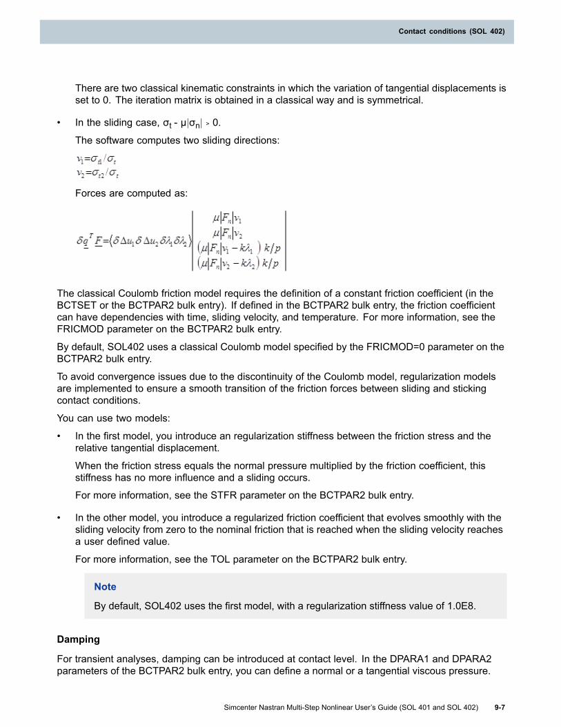
Contact conditions (SOL 402)
There are two classical kinematic constraints in which the variation of tangential displacements isset to 0. The iteration matrix is obtained in a classical way and is symmetrical.
• In the sliding case, σt - μ|σn| ﹥ 0.
The software computes two sliding directions:
Forces are computed as:
The classical Coulomb friction model requires the definition of a constant friction coefficient (in theBCTSET or the BCTPAR2 bulk entry). If defined in the BCTPAR2 bulk entry, the friction coefficientcan have dependencies with time, sliding velocity, and temperature. For more information, see theFRICMOD parameter on the BCTPAR2 bulk entry.
By default, SOL402 uses a classical Coulomb model specified by the FRICMOD=0 parameter on theBCTPAR2 bulk entry.
To avoid convergence issues due to the discontinuity of the Coulomb model, regularization modelsare implemented to ensure a smooth transition of the friction forces between sliding and stickingcontact conditions.
You can use two models:
• In the first model, you introduce an regularization stiffness between the friction stress and therelative tangential displacement.
When the friction stress equals the normal pressure multiplied by the friction coefficient, thisstiffness has no more influence and a sliding occurs.
For more information, see the STFR parameter on the BCTPAR2 bulk entry.
• In the other model, you introduce a regularized friction coefficient that evolves smoothly with thesliding velocity from zero to the nominal friction that is reached when the sliding velocity reachesa user defined value.
For more information, see the TOL parameter on the BCTPAR2 bulk entry.
Note
By default, SOL402 uses the first model, with a regularization stiffness value of 1.0E8.
Damping
For transient analyses, damping can be introduced at contact level. In the DPARA1 and DPARA2parameters of the BCTPAR2 bulk entry, you can define a normal or a tangential viscous pressure.
Simcenter Nastran Multi-Step Nonlinear User’s Guide (SOL 401 and SOL 402) 9-7
Contact conditions (SOL 402)

Chapter 9: Contact conditions (SOL 402)
Those pressures are equal to the product of a function of the normal distance and the velocityassociated to the normal or tangential relative motions.
9.6 Contact and rigid body motionMany static problems rely on contact to provide the boundary conditions necessary for a stableproblem. With these problem types, the stiffness matrix can be singular when the contact constraintsare inactive. You can use the following options to avoid singularities.
• Stiffness stabilization
This feature provides a stabilizing effect by scaling all diagonal stiffness terms without affectingthe right-hand-side load vector. You can request this feature by defining STAB parameter onthe NLCNTL2 bulk entry.
• Displacement scaling
The Newton iteration process can fail to converge if there is an excessive initial incrementaldisplacement. For example, this may occur when contacting surfaces separate. To facilitateconvergence, you can optionally scale down the incremental displacement by defining theexisting parameter MADI on the NLCNTL2 bulk entry. The software uses MADI to compute thedisplacement increment scale factor DSCAL. See DSCAL computation below.
When you define MADI>0.0 (in units of length), the scale factor DSCAL is displayed for eachiteration in the .f06 file in the NEWTON ITERATIONS table. Your choice of the MADI value in asubcase affects how the software calculates DSCAL for each iteration. A suggested value forMADI is 1/4 to 1/3 of the element size.
DSCAL computation
The displacement for the current iteration is approximated by
di=di-1+(DSCAL× Δd)
where,
di is the unknown displacement for the current iteration,
di-1 is the known displacement from the previous successful iteration,
DSCAL is the scaling factor computed by the software,
and Δd is the incremental displacement for the current iteration.
The software computes DSCAL as follows, where Δdmax is the maximum incrementaldisplacement for the current iteration.
o If you define MADI<0.0 (default), the software sets DSCAL=1.0 and no scaling occurs.
o If you define MADI=0.0, the software replaces 0.0 with MADI=0.05 × Lmax, where Lmax isthe distance between the most separated nodes in your model. The software-computedMADI is then used as follows:
■ If MADI<Δdmax, the software sets DSCAL=MADI/(Δdmax+1.0E-10).
■ If MADI>Δdmax, the software sets DSCAL=1.0 and no scaling occurs.
9-8 Simcenter Nastran Multi-Step Nonlinear User’s Guide (SOL 401 and SOL 402)
Chapter 9: Contact conditions (SOL 402)

Contact conditions (SOL 402)
o If you define MADI>0.0, the software uses your MADI definition as follows:
■ If MADI<Δdmax, the software sets DSCAL=MADI/(Δdmax+1.0E-10).
■ If MADI>Δdmax, the software sets DSCAL=1.0 and no scaling occurs.
For more information, see the NLCNTL2 bulk entry in the Simcenter Nastran Quick Reference Guide.
9.7 Contact offsets and initial penetrationsContact surface offsets
Offset can be specified for any contact pair by specifying an offset distance on the associated contactparameter in the BCTPAR2 entry. This causes the actual contact to be shifted from the plane definedby the contact surface nodes. Initial interferences can be modeled using surface contact offsets.
However, specifying offsets on the contact regions (BCRPARA) is not supported by SOL402. Also, forcontact involving shell element faces on one (or both) side(s) of the contact, it is not possible to takeautomatically the offset into account. Instead, the user must manually specify the half-thickness (orthe sum of the half-thicknesses) of the shell(s) as the contact offset.
Initial penetrations
The treatment of initial penetrations is governed by the INIPENE parameter on the BCTPAR2 entry.INIPENE is applied when contact elements are initially created, and if they are recreated as a resultof large displacement effects when PARAM,LGDISP,1 is defined.
• INIPENE = 1 (default): Contact is evaluated exactly as the geometry is modeled. No correctionswill occur for gaps (positive distance between the two contact regions) or penetrations (negativedistance between the two contact regions).
• INIPENE = 2: Only penetrations are reset to a new initial condition in which there is nointerference.
• INIPENE = 3: Both gaps and penetrations are both reset to a new initial condition in whichthere is no interference.
In this case a constant signed gap distance can be defined by GAPVAL, and it will override thegeometrical penetrations and gaps.
• 12: Same as INIPENE=13.
• INIPENE = 13: Gaps and penetrations are both reset to a new initial condition in which thereis an interference provided by GAPVAL for the closest node
For more information, see the BCTPAR2 bulk entry in the Simcenter Nastran Quick Reference Guide.
Simcenter Nastran Multi-Step Nonlinear User’s Guide (SOL 401 and SOL 402) 9-9
Contact conditions (SOL 402)

Chapter 9: Contact conditions (SOL 402)
9.8 Contact convergence
Standard output
The software prints all of the relevant information pertaining to each contact pair at the start of thesolution. For each contact pair BCTSET (referred to as MCT in the f06 file), information on initialgaps/penetrations, characteristic distances, and stiffnesses are provided.
Time step output
Contact change in forces (TESC) are printed as part of the iteration summary.
9-10 Simcenter Nastran Multi-Step Nonlinear User’s Guide (SOL 401 and SOL 402)
Chapter 9: Contact conditions (SOL 402)

Contact conditions (SOL 402)
Convergence considerations
• In the case of convergence issues due to high local contact forces or contact loss, if there areinitial gaps/penetrations in the geometry, setting INIPENE to ignore these would help.
• If the convergence is slow or cannot be achieved for models with friction, using the non-symmetricsolver can improve the convergence rates using the MATSYM parameter on the NLCNTL2bulk entry.
In case of divergence, to help to find the origin of the divergence, a summary of the contact statusduring the iteration is given. The following table is printed in the output file.
Simcenter Nastran Multi-Step Nonlinear User’s Guide (SOL 401 and SOL 402) 9-11
Contact conditions (SOL 402)
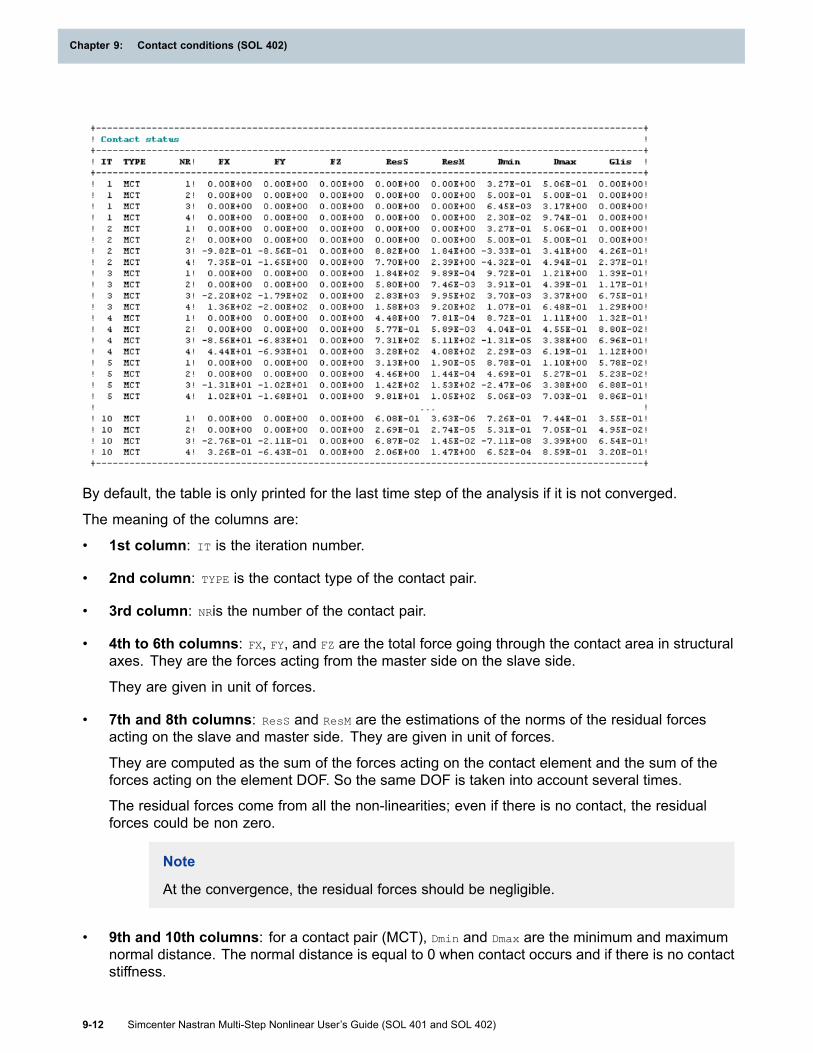
Chapter 9: Contact conditions (SOL 402)
By default, the table is only printed for the last time step of the analysis if it is not converged.
The meaning of the columns are:
• 1st column: IT is the iteration number.
• 2nd column: TYPE is the contact type of the contact pair.
• 3rd column: NRis the number of the contact pair.
• 4th to 6th columns: FX, FY, and FZ are the total force going through the contact area in structuralaxes. They are the forces acting from the master side on the slave side.
They are given in unit of forces.
• 7th and 8th columns: ResS and ResM are the estimations of the norms of the residual forcesacting on the slave and master side. They are given in unit of forces.
They are computed as the sum of the forces acting on the contact element and the sum of theforces acting on the element DOF. So the same DOF is taken into account several times.
The residual forces come from all the non-linearities; even if there is no contact, the residualforces could be non zero.
Note
At the convergence, the residual forces should be negligible.
• 9th and 10th columns: for a contact pair (MCT), Dmin and Dmax are the minimum and maximumnormal distance. The normal distance is equal to 0 when contact occurs and if there is no contactstiffness.
9-12 Simcenter Nastran Multi-Step Nonlinear User’s Guide (SOL 401 and SOL 402)
Chapter 9: Contact conditions (SOL 402)

Contact conditions (SOL 402)
If these values equal 1E12 and –1E12, that means that the slave nodes have no projectionon the master faces.
• 11th column: Glis is the total sliding factor for the contact pair.
By watching the largest values of ResS and ResM, especially in the last iterations, you can discover ifthere is a contact condition for which the residual forces are larger than for the other forces on themodel or for which there are oscillations from one iteration to the next one.
First check if the divergence can be explained by a model weakness (sliding of a free body, and soon) or due to a physical weakness.
In this case, change the contact conditions (consider a larger group of faces, perform a topologysearch at each iteration, introduce contact stiffness, and so on).
9.9 Contact outputContact results can be requested with the BCRESULTS case control command. Forces, tractions,separation distance, total and incremental slide or slip distance, and contact status can be output.
Simcenter Nastran Multi-Step Nonlinear User’s Guide (SOL 401 and SOL 402) 9-13
Contact conditions (SOL 402)


Chapter 10: Glue conditions
10.1 Overview of Gluing ElementsSOL 401 and SOL 402 support the option to glue elements together. Glue is a simple and effectivemethod to join meshes which are dissimilar. It correctly transfers displacement and loads resultingin an accurate strain and stress condition at the interface. The grid points on glued edges andsurfaces do not need to be coincident.
By default, the glue formulation in SOL 401 and SOL 402 creates a connection which preventsrelative motion in all directions.
In SOL 401, you can also optionally turn on the sliding glue formulation for both the surface-to-surfaceand the edge-to-edge glue conditions. Sliding glue includes a normal stiffness but no tangentialstiffness, and is requested by defining the parameter setting SLIDE=1 on the BGPARM entry.
The following table summarizes the supported glue conditions in SOL 401 and SOL 402.
Table 10-1. Glue SummaryType Description
Edge-to-Edge
You can define edge-to-edge glue between the edges of theaxisymmetric elements CTRAX3, CQUADX4, CTRAX6, CQUADX8,plane stress elements CPLSTS3, CPLSTS4, CPLSTS6, CPLSTS8,plane strain elements CPLSTN3, CPLSTN4, CPLSTN6, CPLSTN8,chocking elements CCHOCK3, CCHOCK4, CCHOCK6, CCHOCK8.
Surface-to-Surface
You can define surface-to-surface glue between the faces of thesolid elements CTETRA, CHEXA, CPENTA and CPYRAM, and the shellelements CTRIAR, CQUADR, CTRIA6, and CQUAD8 entries. CQUAD4and CTRIA3 elements are also supported, and the software will treatthem as CQUADR and CTRIAR elements.
Defining Glue Conditions
• Select the glue condition with the BGSET case control command. The BGSET case controlcommand must be above the subcases. As a result, the glue conditions apply to all subcases.See Defining and Selecting Glue Pairs.
• Define source and target regions. See Glue Regions.
• Pair the source and target regions. See Defining and Selecting Glue Pairs.
• Optionally adjust the glue algorithm using glue control parameters. See Glue Control Parameters.
• Optionally request the glue force and traction output with the BGRESULTS case control command.
Simcenter Nastran Multi-Step Nonlinear User’s Guide (SOL 401 and SOL 402) 10-1

Chapter 10: Glue conditions
Edge-to-Edge Glue Summary
• The axisymmetric, plane stress, plane strain, and chocking elements can be defined in either theXZ plane or in the XY plane. Edge-to-edge glue is supported in either orientation.
You create element edge regions with the BEDGE bulk entry. You then pair the regions using thesource and target fields on the BGSET bulk entry.
From the source region, the software searches in the outward normal direction. In addition, thesoftware searches a small distance in the inward normal direction in order to glue edges that mayinterfere due to meshing irregularities. A glue condition is created when a projected normal hitsthe target side, and the distance between the edges is equal to or less than the search distancewhich you specify for the glue pair on the BGSET entry
Surface-to-Surface Glue Summary
Surface-to-surface glue can be defined on the faces of the solid elements CHEXA, CPENTA,CPYRAM, and CTETRA and the shell elements CTRIAR, CQUADR, CTRIA6, and CQUAD8 entries.CQUAD4 and CTRIA3 elements are also supported, and the software will treat them as CQUADRand CTRIAR elements.
You create shell or solid element face regions with the BSURF, BSURFS, BCPROP, or BCPROPSbulk entries. You then pair the regions using the source and target fields on the BGSET bulk entry.From elements in the source region, a normal is projected.
From solid face regions, the software searches in the outward normal direction. In addition, thesoftware searches a small distance in the inward normal direction in order to glue solid faces that mayinterfere due to meshing irregularities.
From shell element face regions, the software searches in both the top and bottom normal directions.
The software creates a glue condition if:
• Any of the source element normals intersect with an element in the target region.
• The distance between the two faces is equal to or less than the search distance which youspecify for the glue pair on the BGSET entry.
Additional information
• When PARM,LGDISP,1 is defined, the glue stiffness orientation will update as a result of largedisplacement effects. The glue stiffness is only computed once, at the beginning of a solution.
• The source side element characteristics are used to define the glue stiffness. Therefore, it ispossible for differences depending on which element faces or edges are selected as the sourceregion.
• The generalized plane strain element is not supported by glue or contact regions.
SOL 402 remarks
• The sliding glue formulation is not available in SOL 402.
• Chocking elements (CCHOCK3, CCHOCK4, CCHOCK6, CCHOCK8) cannot be part of gluingconditions in SOL 402.
10-2 Simcenter Nastran Multi-Step Nonlinear User’s Guide (SOL 401 and SOL 402)
Chapter 10: Glue conditions

Glue conditions
10.2 Glue RegionsThe following describes how edge and surface regions are defined in SOL 401 and SOL 402. Anelement should not appear more than once in the regions that are part of a glue/contact pair. Allregion IDs defined with the BEDGE, BSURFS, or BCPROPS entries must be unique.
Edge Glue Regions
The edge glue region is a selection of axisymmetric, plane strain, plane stress, and chocking elementedges in a section of the model where you expect glue to occur. An element edge is selected on theBEDGE bulk entry by entering the element ID along with the corner GRID IDs.
Surface Glue Regions
A surface glue region is a selection of solid or shell element free faces in a section of the modelwhere you expect glue to occur. These regions can be created using the shell elements (BSURF andBCPROP) and using solid element free faces (BSURFS and BCPROPS).
• The BSURF entry is a list or range of shell element IDs to include in the region.
• The BCPROP entry is a list of shell element property IDs. Shell elements which use any of theselisted property IDs will be included in the region.
• The BSURFS entry is a list of solid element IDs each followed by 3 grid points defining which faceof the 3-D element to include in the glue region.
• The BCPROPS entry is a list of solid element property IDs. The free faces of the solid elementsselected with a property ID are automatically determined by the software.
10.3 Defining and Selecting Glue PairsA glue pair is a way to combine two regions, source and target, in which gluing will be analyzedduring the solution. You use the BGSET bulk entry to define each glue pair. The fields on the BGSETbulk entry are described as follows:
• GSID (glue set id) will need to match the value of ‘n’ on the BGSET case control entry for thesolution to recognize the glue definition.
• SIDi and TIDi are used to select source and target regions for a pair. For surface-to-surfacegluing, they reference the regions created by the BSURF, BSURFS, BCPROP, or BCPROPSentries. For edge-to-edge gluing, they select the regions created by the BEDGE entries. As manypairs as desired can be included on a single BGSET bulk entry.
• SDIST (search distance) defines the distance in which the solver can initially determine if thedistance between element edges or faces in a particular pair are within the threshold for creatingglue elements. The default value of SDIST of 10 is large enough to handle most geometrysituations, but can be adjusted as needed. This value is used once, at the beginning of thesolution, to determine where glue elements are created.
Combining Glue Sets – BGADD
You can optionally define multiple BGSET/BGPARM bulk entry sets, each set with unique glue set IDs(GSID), and then combine them with a single BGADD bulk entry. The multiple BGSET/BGPARM bulk
Simcenter Nastran Multi-Step Nonlinear User’s Guide (SOL 401 and SOL 402) 10-3
Glue conditions

Chapter 10: Glue conditions
entry sets are created to adjust certain glue parameters locally. Glue parameters can also be adjustedglobally with a BGPARM bulk entry having the same GSID as the BGSET case control command.
The following example demonstrates the inputs.
CASE CONTROL$GSID on the BGSET case control matches GSID on BGADDBGSET = 108...BULK DATA$Local Glue Set definitionsBGSET 1 1 2BGSET 2 3 45 6...$Local Glue ParametersBGPARM 1 PENN 80 PENT 80BGPARM 2 PENN 110 PENT 110...$Local Glue Sets are combined with BGADDBGADD 108 1 2...$Global Glue ParametersBGPARM 108 REFINE 0GLUETYPE 1
See the section Glue Control Parameters – BGPARM Bulk Entry in this chapter for more informationon glue parameters.
Gluing Composite Solid Faces
Defining glue regions and pairs on composite solid faces which are perpendicular to the stackdirection (edge faces) may produce poor stress continuity. If the glue definition is between edge facesbelonging to different PCOMPS definitions, and if the number of plies on each PCOMPS definition issmall and the same, and the ply thicknesses are similar, the stress continuity should be fairly smooth.This also applies to the results requested with the BGRESULTS case control command.
Additional Recommendations
When defining glue regions and pairs on geometry which are not tangent continuous, creating singleglue regions which cross corner transitions can result in non-uniform stress results around thecorners. It is recommended to break these areas into multiple regions and pairs as shown below.
10-4 Simcenter Nastran Multi-Step Nonlinear User’s Guide (SOL 401 and SOL 402)
Chapter 10: Glue conditions

Glue conditions
When defining glue regions and pairs, it is recommended to not include the same element face inmultiple regions. In “A” below, an element is repeated in regions 2 and 3. In “B”, the same elementonly exists in region 2. “B” is recommended. Repeating element faces multiple times in the same ordifferent regions can significantly increase memory requirements and degrade performance.
10.4 Glue Control ParametersThe glue control parameters on the BGPARM bulk entry can help you adjust the glue algorithm. Formost solutions, the default settings are appropriate, thus the BGPARM entry is not required.
You can optionally define multiple BGSET/BGPARM bulk entry pairs, each pair with unique glue setIDs (GSID), and then combine them with a single BGADD bulk entry.
The multiple BGSET/BGPARM bulk entry pairs are created to adjust certain glue parameters locally.Glue parameters can also be adjusted globally with a BGPARM bulk entry having the same GSID asthe BGSET case control command.
Global and local glue parameters have the following definition and rules:
• Global Glue Parameters
The BGPARM bulk entry, which uses the same GSID entered on the BGSET case controlcommand, defines global parameters.
For SOL 401, all of the parameters on the BGPARM bulk entry can be defined globally. Aparameter’s default value is used if it is not defined globally or locally.
• Local Glue Parameters
The BGPARM bulk entries associated to individual BGSET bulk entries, which are then combinedwith a BGADD bulk entry, define local parameters.
Simcenter Nastran Multi-Step Nonlinear User’s Guide (SOL 401 and SOL 402) 10-5
Glue conditions

Chapter 10: Glue conditions
For SOL 401, the parameters GLUETYPE, PENN, PENT, PENTYP, PENGLUE, and SLIDE canbe defined locally. A local parameter definition overrides a global definition.
Glue Parameter Descriptions for SOL 401
•
o SOL 401 only supports GLUETYPE=2. As a result, the glue stiffness is determined by thePENTYP and PENGLUE parameters.
PENTYP – Changes the meaning of the PENGLUE parameter as described in the tablebelow. (Default=1)
PENGLUE - A scale factor used to adjust the glue stiffness. (Default=1.0)
PENTYP=1 (Default) PENGLUE is a unitless value (glue stiffness scale factor).PENTYP=2 PENGLUE has the units of F/L2.
Note: For glued coincident faces, there is little flexibility between the faces with default penaltyfactors. The glue condition created between non-coincident faces will not usually produce a localstiffness as accurate as using a conventional finite element for the connection. The flexibility inthe glue condition will depend on the value of the penalty factors. If you have non-coincidentfaces and the glue joint flexibility is important, then it is recommended that you model thisconnection with conventional finite elements.
Average modulus computation
The averaged modulus of the elements associated with the source side region is also used whencomputing the glue stiffness. The averaged modulus is computed as follows.
o The modulus is averaged for the elements associated with the source side region.
o For elements using orthotropic and anisotropic materials, the element modulus value used inthe average modulus computation is computed as follows.
MAT9: E=(C11+C22+C33)/3
MAT11: E= (E1+E2+E3)/3
o When a solid composite defined with the PCOMPS entry is included in a source glue region,the average modulus is computed by averaging all modulus values defined on all materialsdefined in the input file.
• SLIDE - Requests the sliding glue. Sliding glue includes normal stiffness but no tangentialstiffness. Gaps between the glued surfaces are preserved as sliding occurs.
0 - Sliding glue is off (default).
1 - Sliding glue is on.
• INTORD and REFINE help to improve the accuracy of the glue solution. The number oflocations where normals are projected (glue points) from the source region is dependent on thevalue assigned to the INTORD parameter, and on the element face type. The following tablesummarizes how the INTORD value adjusts the number of glue points for a particular elementface:
10-6 Simcenter Nastran Multi-Step Nonlinear User’s Guide (SOL 401 and SOL 402)
Chapter 10: Glue conditions

Glue conditions
Number of Glue Points Used in Glue Element EvaluationFace Type INTORD=1 INTORD=2 (default) INTORD=3Linear Triangle 1 3 7Parabolic Triangle 3 7 12Linear Quad 1 4 9Parabolic Quad 4 9 16
REFINE will increase the number of glue points by refining the mesh on the source region. Partof the refinement process is to project element edges and grids from the associated target regionback to the source region. The resulting refinement on the source region is then more consistentwith the target side, which then gives a better distribution of glue elements. The refined grids andelements are only used during the solution. The glue results are transferred back to the originalmesh for post processing results.
Refinement occurs when set to 2 (default). REFINE=0 turns the refinement off.
• You can use the PREVIEW parameter to request the export of a bulk data representation of theelement edges and faces where glue elements are created. See Glue Preview.
Glue Parameter Descriptions for SOL 402
1. SOL 402 only supports BGOPT. Other parameters are ignored. The glue is therefore always aperfect weld glue (GLUETYPE=2).
The BGOPT parameter must be defined as a local parameter. The BGPARM bulk entriesassociated to individual BGSET bulk entries, which are then combined with a BGADD bulkentry, define local parameters.
2. The BGOPT parameter adds a rotation constraint on the DOFs of the source nodes. You canchoose between the following options:
• You can let the software automatically choose the best option according to the source andtarget region configurations that you defined for the glue pair (default).
• You can fully unconstrain the rotations.
• You can constrain the source nodal rotations using the target nodal rotations. This option canbe used for instance when you glue two regions of shells.
• You can constrain the source nodal rotations using target mean nodal displacements. Thisoption can be used, for example, when you glue shells to faces of volumes.
3. The following table describes the available options FOR BGOPT according to the source andtarget regions defined in the glue set GSID (BGSET entry).
Glue Type Source Target Allowed BGOPT values
Edge-to-Edge Glue BEDGE BEDGE
1
2
0 (default); same as BGOPT=2
Simcenter Nastran Multi-Step Nonlinear User’s Guide (SOL 401 and SOL 402) 10-7
Glue conditions

Chapter 10: Glue conditions
Glue Type Source Target Allowed BGOPT values
Edge-to-Surface Glue BEDGE BSURF
2
3
0 (default); same as BGOPT=3
BSURF BSURF
1
2
3
0 (default); same as BGOPT=3Surface-to-Surface Glue
BSURF BSURFS
1
3
0 (default); same BGOPT=3
For the following source and target combinations, the BGOPT option is ignored.
Glue Type Source TargetBSURFS BEDGEEdge-to-Surface GlueBEDGE BSURFSBSURFS BSURFS
Surface-to-Surface GlueBSURFS BSURF
10.5 Glue previewYou can optionally export a bulk data representation of the element edges and faces where glueconditions are created. To do so, set the PREVIEW parameter on the BGPARM bulk entry to “1”.For example:
$*BGSET 100 1 2 0.001000BGPARM 100 PREVIEW 1$*
The software writes a bulk data file containing dummy shell element entries for face locations, anddummy PLOTEL entries for edge locations. Dummy GRID, property, and material entries are alsowritten. You can import the file into a preprocessor to display both source and target glue locations.
The preview file has the naming convention:
<input_file_name>_glue_preview_<subcaseid>_<gluesetid>.dat
For example, if an input file named test.dat includes a subcase numbered 101 and a glue setnumbered 201, the resulting preview file name is:
test_glue_preview_101_201.dat
In the following simple example, the red mesh is glued to the green.
10-8 Simcenter Nastran Multi-Step Nonlinear User’s Guide (SOL 401 and SOL 402)
Chapter 10: Glue conditions

Glue conditions
Before applying any loading, the software creates the glue elements. This is the point in the solutionin which the preview output is written.
The following illustration shows how the preview appears after you import the preview file into theSimcenter preprocessor. Note that the colors were manually modified in Simcenter after importingthe file.
Simcenter Nastran Multi-Step Nonlinear User’s Guide (SOL 401 and SOL 402) 10-9
Glue conditions


Chapter 11: Considerations for nonlinear analysis
11.1 Discrete system for a nonlinear continuum modelTheories in solid mechanics are dictated by three governing relationships:
• The state equilibrium that
Equation 11-1.
requires where σij are stress tensor components, bi are body forces, and xj are space coordinates.
• The constitutive relations represented by stress-strain relations, e.g., for linear elasticity,
Equation 11-2.
where εkl are strain tensor components and Dijkl are elastic constants.
• The compatibility represented by strain-displacement relations, e.g., for a small deformation,
Equation 11-3.
where ui are displacements.
These systems of governing differential equations must be satisfied for every infinitesimal elementthroughout the domain of the continuum. The complete set of state variables, namely displacements,may be determined by solving these systems of equations supplemented by boundary conditions,and in dynamic situations by initial conditions as well. For the nonlinear problems, the governingequations should be satisfied throughout the history of load application. The material nonlinearityis manifested in the constitutive relations. The geometric nonlinearity is pronounced in thestrain-displacement relations, but it also affects the equilibrium equation by changing applied loads.Changes in constraints affect the boundary conditions, which constitute contact problems.
Most of the known solutions for the solid mechanics problems are based on ideal geometry and linearapproximations. However, the real nature is more complicated and inherently nonlinear. The linearsystem is a very particular case of a general problem. Even the nonlinear solutions that we seek dealwith only a small subset of special cases in a general category of nonlinear problems. When the
Simcenter Nastran Multi-Step Nonlinear User’s Guide (SOL 401 and SOL 402) 11-1

Chapter 11: Considerations for nonlinear analysis
nonlinear system is confronted, no general mathematical solutions exist and superposition no longerapplies. The system may even be non-conservative.
The first phase of the structural analysis is the idealization of a physical system into a simpler andmore manageable engineering problem. The idealization process involves simplifications of thegeometry, boundary and joint conditions, and loading conditions, etc. using engineering intuitions,experimental data, empirical observations, and classical solutions. If the idealized structural systemrenders a problem that cannot be resorted to a classical method of analysis, further idealization isrequired, namely discretization, for numerical analysis.
Finite elements represent spatial discretization of a continuum. As such, however, they donot immediately impose nonlinearity. When nonlinearity has to be taken into account for largedisplacements and/or stresses, a numerical model poses new dimensions to the discretization inaddition to the n-dimensional Euclidean space. That is, the discretization is applied to time, load,and material properties by using piece wise linear curves. While discretization allows approximatesolutions by numerical methods, it introduces numerous mathematical singularities which maycomplicate computational processes. Fortunately, the efficiency of modern digital computers makesit feasible to apply complicated computational procedures to the complex systems of engineeringproblems.
For the discrete system, governing differential equations are converted to algebraic equations. Thefinite element model represents a structure by an assemblage of finite elements interconnected atnodal points. State variables are the displacements (displacement method or stiffness approach.) ofthe nodal points which carry fictitious forces representing distributed stresses actually acting on theelement boundaries. The equilibrium requirements are satisfied at nodal points by the nodal forcebalance. The material constitutive laws are satisfied at the integration points of the element. Thecompatibility is ensured by the displacement continuity between elements. It is noted, however, thatthe compatibility of the nonconforming elements is ensured by a patch test.
11.2 Finite element formulation for equilibrium equationsThe variational principle renders the system governing equilibrium equations when applied to afunctional ll, representing a total potential of a continuum, i.e.,
Equation 11-4.
where U is the strain energy of the system and W is the potential energy of the external loads. Theequilibrium equations can be obtained by invoking the principle of virtual work or the Ritz method, i.e.,
Equation 11-5.
which implies that the total potential of the system must be stationary with respect to the statevariables (displacement) for equilibrium to be ensured. The functional IT is so called because itinvolves the integral of implicit functions of the state variables, {u}.
11-2 Simcenter Nastran Multi-Step Nonlinear User’s Guide (SOL 401 and SOL 402)
Chapter 11: Considerations for nonlinear analysis

Considerations for nonlinear analysis
Considering a three-dimensional continuum for a nonlinear problem, the stationarity condition resultsin
Equation 11-6.
where the dots and δ denote infinitesimal increments and arbitrary variations, respectively. Theleft-hand side represents variations in the strain energy increment and the right-hand side representsvariations in the external work which consists of body forces bi (such as a gravity load), traction forcesti at the boundary surface (such as pressure loads), and concentrated forces pi. Now it remainsto determine admissible functions expressing the arguments of the functional II in terms of statevariables {u}, which are valid throughout the whole region and satisfy the boundary conditions.
The finite element method can be characterized by the following features distinguished from theconventional Ritz methods or the matrix method for frame structures:
• The whole region of the system is divided into numerous subdomains, called finite elements,which have simple geometrical shapes.
• The variational process is limited to each finite element, which aggregates into a whole regionwhen assembled.
• The admissible displacement field within each element, , can be expressed in terms of nodaldisplacements using interpolation functions known as shape functions, N, i.e.,
Equation 11-7.
where {u} is a displacement vector consisting of all nodal points of the element.
The strain-displacement relations for the element can then be established in terms of nodaldisplacements using the shape functions in Equation 11-7, i.e.,
Equation 11-8.
where
Equation 11-9.
and the element matrix [B] consists of derivatives of the shape functions, evaluated at the currentdeformed geometry. Notice that the geometric linear problem requires that the element matrix beevaluated only at the initial geometry. The software employs an approximate updated Lagrangianapproach for geometric nonlinear problems, by which linear strains are computed in the updatedelement coordinate system in order to eliminate the effects of the rigid body rotation but the
Simcenter Nastran Multi-Step Nonlinear User’s Guide (SOL 401 and SOL 402) 11-3
Considerations for nonlinear analysis

Chapter 11: Considerations for nonlinear analysis
equilibrium is established at the final position in the stationary coordinate system. This method doesnot require reevaluation of the element matrix [B] (constant in the absence of large strains) while theelement coordinates are reevaluated continuously.
Equilibrium equations for an element may be obtained by reducing Equation 11-6 after the substitutionof Equations 11-7 and 11-8, based on the small deformation theory. Then the element boundarystresses are statically equivalent to the nodal forces which balance the applied external loads, i.e.,
Equation 11-10.
with
Equation 11-11.
and
Equation 11-12.
where [Ns] is an appropriate interpolation function for the traction force. Notice that the equilibriumequation for an incremental load may be expressed as
Equation 11-13.
where should be components of co-rotational stress which is independent of a rigid body rotation.
The element stiffness matrix can be obtained by substituting the constitutive relations into Equation11-13, i.e.,
Equation 11-14.
where
Equation 11-15.
and [D] is the material tangent matrix. The nodal forces of an element can then be expressed as
11-4 Simcenter Nastran Multi-Step Nonlinear User’s Guide (SOL 401 and SOL 402)
Chapter 11: Considerations for nonlinear analysis

Considerations for nonlinear analysis
Equation 11-16.
where the element stiffness is
Equation 11-17.
Notice that this expression represents an element stiffness due to the material stiffness withoutgeometric nonlinear effects. As will be shown later, an additional stiffness [J(d)] due to initial stressesshould be included for an incremental process because the initial stresses exist from the secondincrement.
The equilibrium must be satisfied in the whole region throughout the complete history of loadapplication. Equilibrium equations for the global discrete system are obtained when all the elementsare assembled, i.e.,
Equation 11-18.
where Σ over m denotes a summation over all elements. For the incremental process, the equilibriumequation may be rewritten as
Equation 11-19.
with
Equation 11-20.
where {σ0} represents an initial stress or the stress state at the preceding load step.
Because of the approximations involved in the interpolation functions, the finite element modelprovides an approximate solution even if the equilibrium Equation 11-18 is satisfied exactly.Consequently, the differential equations of equilibrium are not satisfied exactly even for linearproblems, but the error decreases as the finite element mesh is refined. This convergence conditionis required and ensured by element formulations with regard to the element convergence criteria.
Simcenter Nastran Multi-Step Nonlinear User’s Guide (SOL 401 and SOL 402) 11-5
Considerations for nonlinear analysis

Chapter 11: Considerations for nonlinear analysis
11.3 Coordinate transformationsThe coordinate transformation is one of the most frequent operations in the finite element method.Vectors and matrices defined in a particular coordinate system can be transformed into anothersystem. Coordinate systems involved are:
• Basic coordinate system: a Cartesian coordinate system on which local coordinate systemsare defined.
• Local coordinate system: defined by the user in the Bulk Data, which may include specialcoordinates such as cylindrical and spherical coordinate systems.
• Global coordinate system: a collective coordinate system which comprises all the local coordinatesystems specified for output quantities.
• Element coordinate system: a Cartesian coordinate system unique to each element.
• Displaced element coordinate system: similar to element coordinate system but defined in thedisplaced position.
• Material coordinate system: a Cartesian coordinate system used to orient anisotropic materialproperties.
• Modal coordinate system: a generalized coordinate system defined for each eigenmode.
It is noted that the global system is a Cartesian coordinate system, although non-Cartesian coordinatesystems are adopted to orient the local Cartesian coordinates for output quantities. In the software,all the displacements and forces, hence the system matrices, such as the stiffness matrix, areexpressed in the global coordinates. This implies that all the major computations involved in theanalysis are processed in Cartesian coordinates. Element and material coordinate systems aredefined in the element connectivity description. Now we only have to consider linear transformationsbetween Cartesian coordinate systems.
Let us consider a coordinate transformation between the primed and unprimed systems which areright-handed Cartesian coordinates. The transformation matrix T consists of direction cosines of unitvectors of the unprimed coordinate system, i.e.,
Equation 11-21.
where
Equation 11-22.
Notice that T is an orthogonal matrix and thus
11-6 Simcenter Nastran Multi-Step Nonlinear User’s Guide (SOL 401 and SOL 402)
Chapter 11: Considerations for nonlinear analysis

Considerations for nonlinear analysis
Equation 11-23.
Because the work and energy are invariants with respect to coordinate transformation, i.e.,
Equation 11-24.
it follows that
Equation 11-25.
Then the equilibrium equation,
Equation 11-26.
may be expressed in the unprimed coordinate system by
Equation 11-27.
with
Equation 11-28.
It is noted that the modal matrix Φ is used as a transformation matrix for a modal transformationwhich is not elaborated here.
Equation 11-29.
The forces and displacements are transformed from element to global coordinates and vice versa, i.e.
where Tbe transforms from element to basic coordinates and Tbg transforms from global to basiccoordinates.
It is noted that Tbe is identical for all the nodes of an element but Tbg may vary from node to node inthe same element. The element stiffness matrix is transformed into global coordinates by
Simcenter Nastran Multi-Step Nonlinear User’s Guide (SOL 401 and SOL 402) 11-7
Considerations for nonlinear analysis

Chapter 11: Considerations for nonlinear analysis
Equation 11-30.
for which the building blocks of Tbe and Tbg are (3x3) matrices formed for each nodal point and haveto be assembled for an entire element, e.g. for a three-noded triangular shell element
Equation 11-31.
where the superscript is used to associate each (3x3) matrix with the nodal point and is repeatedfor the rotational degrees of freedom.
11.4 Displacement sets and reduction of system equationsThe equilibrium equations, and thus system matrices, are reduced in size using the displacement set,which is a unique feature of this software. Mutually exclusive subsets of the global displacement set,{ug}, are defined as follows:
um Degrees-of-freedom eliminated by multipoint constraints
us Degrees-of-freedom eliminated by single-point constraints
uo Degrees-of-freedom omitted by static condensation
ur Degrees-of-freedom eliminated by a bulk data SUPORT to suppress rigidbody motion
ui Degrees-of-freedom which remain for solution after reductions
For convenience, complementary sets are defined as follows:
un = ug - umuf = un - usua = uf - uoul = ua - urThe subsets are defined by the user with a possible exception in the s-set if PARAM,AUTOSPC,YESis used. Notice that the rigid elements are equivalent to the multipoint constraints internally in theprogram, but they are not selectable in the subcases as for MPCs. Because the set-reductionoperations involve many basic modules and DMAP blocks, the mathematics for elimination ofconstraints and static condensation is reviewed here.
The multipoint constraint equations are formed in the module GP4 as follows:
11-8 Simcenter Nastran Multi-Step Nonlinear User’s Guide (SOL 401 and SOL 402)
Chapter 11: Considerations for nonlinear analysis

Considerations for nonlinear analysis
Equation 11-32.
where
The module MCE1 partitions [Rmg] and solves for a transformation matrix [Gmn], i.e.,
Equation 11-33.
where
Then the module MCE2 partitions the global stiffness matrix, [Kgg], and reduce it to the n-set, i.e.,
Equation 11-34.
from which the system is reduced to
Equation 11-35.
where
and
The primes are used in K’nn, P’n, and Q’n to distinguish from Knn, Pn, and Qn, which are resultingmatrices after the reduction.
Equations in the n-set can be further reduced by eliminating single-point constraints, i.e.,
Equation 11-36.
Simcenter Nastran Multi-Step Nonlinear User’s Guide (SOL 401 and SOL 402) 11-9
Considerations for nonlinear analysis

Chapter 11: Considerations for nonlinear analysis
which is reduced to
Equation 11-37.
where
with
Notice that the effects of constraint forces (Qs and Qm) are not visible in Equation 11-37. Thesingle-point constraint forces are recovered by
Equation 11-38.
Further reduction of equations in the f-set is performed by an elimination of the o-set, known as staticcondensation. The f-set is partitioned by the UPARTN module as follows:
Equation 11-39.
from which
Equation 11-40.
where
and
Then the reduced system of equations in the a-set is obtained as
Equation 11-41.
where
and
11-10 Simcenter Nastran Multi-Step Nonlinear User’s Guide (SOL 401 and SOL 402)
Chapter 11: Considerations for nonlinear analysis

Considerations for nonlinear analysis
There are some rules to remember regarding the displacement sets in SOL 401. They are:
• The r-set is not supported. Do not use the SUPORT bulk entry.
• PARAM, AUTOSPC is not supported.
• PARAM, AUTOSPCR is not supported.
• Rigid elements are formulated with linear multipoint constraint equations and do not have largedisplacement capability. Consequently, erroneous results will be obtained if the rigid elementundergoes a large rotation. To avoid this, stiff elements should be used in place of rigid elementsfor large displacement analysis.
11.5 Nonlinear solution procedureThe general-purpose program developer faces the task of providing the best workable solutionmethod for a wide spectrum of problems, while maintaining flexibility by allowing the user to specifyoptional parameters. Based on the extensive numerical experiments, an attempt was made toestablish a general strategy suitable for most problems without requiring insight or experience.Variations in combining theories, algorithms, criteria and parameter values with numerous testproblems resulted in a succinct implementation.
The major feature of the nonlinear analysis is the requirement for the incremental and iterativeprocesses to obtain a solution. The main issue is how to choose the most efficient method from theoptions available for the incremental and iterative processes in the solution of nonlinear equilibriumequations. The increment size for time steps has the most significant effect on the efficiency andthe accuracy of the computation, particularly in the path-dependent problems. The incremental anditerative processes are complementary to each other because the larger the increment size themore iterations the solution requires. While an excessively small increment reduces the computingefficiency without any significant improvement in accuracy, a large increment may deteriorate theefficiency as well as the accuracy; it may even cause divergence.
It is impossible to optimize the incremental step size in the absence of prior knowledge of thestructural response. The best engineering judgement should be exercised to determine the incrementsize based on the severity of the nonlinearity. Needless to say, no incremental load steps are requiredwhen the response is linear. In principle, the size of the load increment (or time increment) should bechosen to yield a uniform rate of change in strains or stresses for the material nonlinear problems anda uniform rate of change in displacements for geometric nonlinear problems.
Specifying nonlinear analyses parameters in SOL 401
User specifications for solution methods in nonlinear analyses are allowed via:
• The NLCNTL bulk entry for the static analysis. It is selected by the NLCNTL case controlcommand.
• The TSTEP and TSTEP1 bulk entries for the load increment (time-based). It is selected by theTSTEPNL case control command.
Simcenter Nastran Multi-Step Nonlinear User’s Guide (SOL 401 and SOL 402) 11-11
Considerations for nonlinear analysis

Chapter 11: Considerations for nonlinear analysis
The increment size can vary from subcase to subcase by specifying different TSTEPNL. It isrecommended that you define separate TSTEPNL for every subcase even if the same values arespecified, so that changes can be accommodated at the subcase level as needed.
See also Time step intervals
• The EIGRL bulk entry for the modal analysis. It is selected by the METHOD case controlcommand.
Specifying nonlinear analyses parameters in SOL 402
Solution control parameters
You can define solution control parameters either globally (NLCNTLG bulk entry) or by subcase(NLCNTL2 bulk entry).
On the NLCNTLG bulk entry:
• You can select the solver type (skyline, sparse or parallel).
• You can select the stress-strain measure for all material laws (Kirchoff, Cauchy, Biot, Green,or log).
• You can choose the type of initial and/or steady-state computation.
On the NLCNTL2 bulk entry:
• You can choose between fixed time steps or automatic time stepping. You can also control thetime step size (minimum, maximum, increase ratio).
• You can control the equilibrium iteration and convergence of the solution.
• You can define the time integration scheme (Newmark, HHT, or Generalized-alpha) forDYNAMICS subcases. You can also control the integration error.
• For a non-sequentially dependent (NSD) static subcase (SEQDEP=NO), you can optionallyreload the computation state from the end of a previous subcase using the RSUB=n parameter.
For more information, see Subcase sequencing.
Time step intervals
The TSTEP1 bulk entry defines the time step intervals at which a solution will be generated and output:
• It applies to time-based subcases: ANALYSIS=STATICS in SOL 401, ANALYSIS=STATICS andANALYSIS=DYNAMICS in SOL 402.
• It applies to load-factor-based subcases: ANALYSIS=PRELOAD in SOL 402.
• It is not used for modal subcases (MODES, CYCMODES, FOURIER, and BUCKLING).
• In SOL 401, the start time (Tstart) for a time-based subcase depends on its sequentialdependency. See the SEQDEP bulk entry.
In SOL 402, the start time is always the end time of the previous subcase, regardless of thesequential dependency.
11-12 Simcenter Nastran Multi-Step Nonlinear User’s Guide (SOL 401 and SOL 402)
Chapter 11: Considerations for nonlinear analysis

Considerations for nonlinear analysis
In SOL 401, you can also use the TSTEP bulk entry. The use of TSTEP in SOL 402 is notrecommended
11.6 SOL 401 RestartA restart solution is a method of continuing from a previous run without having to start from thebeginning. For example, an initial run could be a pre-stressed condition which includes a bolt preloadsubcase and multiple static subcases. You can then use the restart file created from the initial run inrepeated restart solutions.
The restart solution is also useful when a solution fails to converge. The software saves thecompleted solution points up to the failed time point. When restarting, you can reduce the size of yoursolution increments or perhaps adjust the nonlinear control parameters to help convergence.
For the restart run, you can change load, SPC, MPC, element birth/death, contact, and subcasedefined nonlinear control parameters. By default, you cannot create new grid points or elements,change grid point locations, change glue conditions, or modify materials. See Model check.
Initial run
The initial solution input file can include any combination of static, dynamic, and preload subcasetypes. The modal, cyclic, Fourier subcase types, and nonlinear buckling are not supported in theinitial run.
For the initial run, when you include the parameter definition RSTGEN=YES on the NLCNTLG bulkentry, the software writes restart data to the same .op2 file in which results are written. The .op2 fileproduced from the initial run will include saved restart solution points from the end of each static,dynamic, and preload subcase. In addition, if convergence fails in a static or dynamic subcase, arestart point is written from the last converged time step. If a preload subcase fails to converge, norestart point is written for that subcase. A preload subcase must complete for a restart point tobe written.
For example, the following input file structure includes the parameter definition RSTGEN=YES onthe NLCNTLG bulk entry to request restart data. If all three subcases complete, restart data willbe written to the .op2 file at the end of each.
....LGDISP=1SUBCASE 1ANALYSIS=PRELOADSUBCASE 2ANALYSIS=STATICSSUBCASE 3ANALYSIS=STATICS....BULK DATANLCNTLG,RSTGEN,YES....
When you request an initial solution with RSTGEN = YES, the .op2 file is always written as 64-bit,and the parameter OP2FMT is ignored.
Restart run
Simcenter Nastran Multi-Step Nonlinear User’s Guide (SOL 401 and SOL 402) 11-13
Considerations for nonlinear analysis

Chapter 11: Considerations for nonlinear analysis
In your restart input file, you will include an ASSIGN statement that references the .op2 file createdfrom the initial solution. The ASSIGN statement must include a unit number of 161 or larger. Inaddition, if the unit number on your ASSIGN statement is not 161, you must define the parameterRSTUNIT=unit number on the NLCNTLG bulk entry.
Example one:
ASSIGN INPUTT2='OUTDIR:restart_op2_filename.op2' UNIT=161....BULK DATA***NLCNTLG,RSTUNIT is not required for this example since UNIT=161**....
Example two:
ASSIGN INPUTT2='OUTDIR:restart_op2_filename.op2' UNIT=201....BULK DATANLCNTLG,RSTUNIT,201***NLCNTLG,RSTUNIT is required for this example since UNIT>161**....
If your restart run input file has the same name as your initial run input file, you should rename the.op2 file created from the initial run if you want to preserve it. Otherwise, it will be overwritten duringthe restart solution. Your ASSIGN statement should also refect the new .op2 file name.
The .op2 file created from the initial run can include saved restart solution points from multiplesubcases. For the restart run, you use the parameter RSTFROM=n on the NLCNTLG bulk entry toselect which initial subcase ID to restart from. Since the RSTFROM=n parameter has no default, itis required.
The start time for a restart solution is always the end or final time of the solution point you arerestarting from. For example, let us assume your initial solution included a subcase 1 with time goingfrom 0.0 to 10.0 seconds, a subcase 2 with time going from 10.0 to 30.0 seconds, and all time stepsconverged successfully for each subcase. If you restart from subcase 2, the start time will be 30.0seconds. If your first subcase in the restart input file includes a TSTEP1 bulk entry with an end time of40 seconds, and a number of increments of 5, the time steps for this restart subcase will be 32.0,34.0, 36.0, 38.0, and 40.0 seconds.
The number of subcases and their IDs in the restart input file can be the same as those used in theinitial run, or they can be completely different. You use the parameter EXEFROM=n on the NLCNTLGbulk entry to select a subcase ID in the restart run input file in which to begin the restart solution.Since the EXEFROM=n parameter has no default, it is required. The software automatically makesthe subcase you select with EXEFROM=n sequentially dependent on the subcase you select withRSTFROM=n, even if SEQDEP=NO is defined in the subcase selected by EXEFROM=n.
For example, suppose your initial run included three subcases with IDs 1, 2, and 3, all threecompleted, and you have decided to restart from the initial subcase 2 by defining the parameterRSTFROM=2 in your restart input file. In addition, your restart input file has the subcase IDs 1, 3, 5,and 7 and you would like to begin the restart solution with subcase 5. As a result, you will also defineEXEFROM=5 in your restart input file. See Special case: EXEFROM=RSTFROM below.
You can request restart data from a restart run by including the parameter definition RSTGEN=YESon the NLCNTLG bulk entry in the restart run input file. This is useful when convergence problemsare occuring. With each consecutive restart, you are saving the solution progress.
11-14 Simcenter Nastran Multi-Step Nonlinear User’s Guide (SOL 401 and SOL 402)
Chapter 11: Considerations for nonlinear analysis

Considerations for nonlinear analysis
You can define any of the subcase types in the restart input file. Although, if the subcase youselect with RSTFROM is a dynamics subcase, the subcase you select with EXEFROM cannot bea modal, cyclic, or Fourier.
In all restart runs, the software copies the results from the initial run .op2 file into the .op2 file createdin the restart run. As a result, the restart .op2 will include both the initial run subcase results and therestart run subcase results. The software automatically relabels any subcase IDs if a conflict occursbetween the initial run subcase IDs and the restart run subcase IDs.
If you are unsure of the resulting subcase IDs and the time steps in a restart .op2 file, you can loadthe .op2 file into Simcenter 3D post processing. The Post Processing Navigator organizes theresults according to subcase ID and time step.
Special case: EXEFROM = RSTFROM
The purpose of this special case is to continue a non-converged subcase. Only the solution controlparameters on the NLCNTL bulk entry and the time step intervals on the TSTEP1 bulk entry canchange from the initial run to the restart run.
Specifically:
• The TSTEP1 entry defined for the first subcase in the restart input file must have the same endtime as the end time defined for the non-converging subcase in the initial run. The Ninc and Noutfields that define the time step intervals and output are applied from the start time to Tend.
• Any new or modified solution control parameters defined on the NLCNTL entry in the restartinput file apply only from the start time to Tend.
• To keep compatibility with the initial run, the general solution parameters LVAR, TVAR, THRMST,and LOADOFF that are related to loading cannot change.
Model check
By default, during the restart solution, a model check occurs that compares the model data in therestart input file with the model data stored from the initial run .op2 file. A fatal error will occur if modeldifferences are found. There are exceptions where the model may need to be modified. For example,you may need to add a spring element to help a failing solution complete. The parameter MDLVAL onthe NLCNTLG bulk entry is available to turn the model check off.
You can remove all model data from the restart input file and the model validation will be skipped. Forthis case, the software uses the model data in the initial run .op2 file.
Restart parameter summary:
RSTGEN For the initial run, requests that restart data will be saved forstatic, dynamic, and preload subcases. SOL 401 saves therestart data in the output OP2 file. (Character; Default = NO).
YES = Restart data is saved.
NO = Restart data is not saved.
Simcenter Nastran Multi-Step Nonlinear User’s Guide (SOL 401 and SOL 402) 11-15
Considerations for nonlinear analysis

Chapter 11: Considerations for nonlinear analysis
RSTUNIT=n For the restart run, defines the unit number of the external restartfile. The unit number must also be specified on an ASSIGNstatement that references the physical filename of the .op2.(Integer≥161; Default=161)
RSTFROM =n For the restart run, defines the subcase ID from which torestart. This subcase ID was defined in the initial run input file.RSTFROM has no default and must be defined. (Integer>0; Nodefault).
EXEFROM = n For the restart run, defines the subcase ID from which to execute.This subcase ID is defined in the restart run input file. EXEFROMhas no default and must be defined. (Integer>0; No default)
MDLVAL For the restart run, allows the option to turn off the modelvalidation check (Character; Default = “YES”).
YES = Request model validation.
NO = Do not request model validation.
11.7 SOL 402 RestartRestarting solutions saves solving time by letting you reuse previously computed results. You canuse the previously computed results to start subcases within the same solution (internal restarts), oryou can use them to start new solutions (external restarts).
Internal restarts (SOL 402 only)
Internal restarts start a specified subcase with the computation state (displacements, velocities,stresses, state variables, and so on) of a preload, static, or dynamic subcase during the same solve.For example, you might want to start several non-sequentially dependent (NSD) subcases with theresults of a bolt preload subcase. Similarly, you can start other NSD subcases with the results ofa dynamics subcase.
You can use the RSUB=n parameter of the NLCNTL2 bulk entry to make an internal restart.
Although these subcases restart with computation state of the subcase you specify, they do notrestart with the end time of the specified subcase. Time continues to increment for each subcase.
External restarts
External restarts start a new nonlinear solve with results from a previous solve. For example, you canstart a new solution using the computed pre-stress of your model. Or, you can start a new solutionfrom the last converged step within a static or dynamic subcase.
SOL 402 supports external restarts from the end of a subcase or from the last converged timestep. It does not support restarting from other time steps within a subcase. The restart point canbe a static subcase, dynamic subcase, or the end of preload subcase. Your restart solution canbe a clone of your initial run solution (preferred method), or it can be a new solution (in this caseyou do not refer to the initial solution).
11-16 Simcenter Nastran Multi-Step Nonlinear User’s Guide (SOL 401 and SOL 402)
Chapter 11: Considerations for nonlinear analysis

Considerations for nonlinear analysis
Saving the restart data at the initial run
If you plan to make a restart, you must first save the restart data during the initial run.
You do this with the RSTGEN=YES parameter of the NLCNTLG bulk entry. All the subcases of thatrun will be potential subcases for a future restart.
For SOL 402, the data is saved in the output OP2 file, the Samcef .sdb and .adb database files, andthe Samcef output .u18 file.
The restart run
In the restart run:
• You must specify the subcase ID from which you restart. You do this with the RSTFROMparameter of the NLCNTLG bulk entry.
See also the RSTFROM parameter.
• You must specify the subcase ID from which you execute. You do this with the EXEFROMparameter of the NLCNTLG bulk entry.
See also the EXEFROM parameter.
• You must also specify the unit of that external restart file. You do this with the RSTUNITparameter of the NLCNTLG bulk entry.
The unit number must also be specified on an ASSIGN statement that references the physical filename of the initial .op2 file.
Example
ASSIGN inputt2='OUTDIR:k402.op2' unit=170 status=unknown....NLCNTLG RSTUNIT 170 RSTFROM 1 EXEFROM 2
The subcase ID from which you restart (RSTFROM)
RSTFROM specifies the subcase ID from which you restart.
The restart solution uses the restart subcases that precede or equal the specified subcase.
• If you cloned the initial run solution to be your restart solution, the restart solution has the samesubcase ID numbers of the initial run solution. Therefore, the restart subcases in the initial run.op2 file replace the same numbered subcases in the restart solution starting with the subcaseyou select here. For example, if three restart subcases are available and you select subcase 2,the solution starts with the end state of subcase 2 and recomputes subcase 3.
• If you created a new restart solution, the restart solution starts from the end subcase you specifybut the new subcase will be numbered from 1 again. All restart subcases prior to the one youselect are included in the solution. For example, if the initial run .op2 file contains five subcasesand you specify subcase 3 as the subcase from which to restart the solution, subcases 1, 2, and3 are included in the restart solution, but subcases 4 and 5 are not.
Simcenter Nastran Multi-Step Nonlinear User’s Guide (SOL 401 and SOL 402) 11-17
Considerations for nonlinear analysis
Chapter 11: Considerations for nonlinear analysis
The subcase ID from which you execute (EXEFROM)
EXEFROM specifies the subcase ID from which you execute.
For example, if the initial run .op2 file contains five subcases and you specify RSTFROM=3 andEXEFROM=4 in the restart solution, your restart solution executes from the subcase 4 and uses therestart data of the subcase 3 of the initial run.
Model validation for the restart run
SOL 402 does not allow you to add or remove elements, materials, boundary conditions, and so onin the restart run model. At most, you can change solution parameters or the numerical values ofthe boundary conditions. The MDLVAL parameter of the NLCNTLG bulk entry, therefore, doesnot apply to SOL 402.
11.8 Stress-strain measures (SOL 402)In SOL 402, in the NLCNTLG bulk entry, you can specify stress-strain measures for plastic materiallaws and measures for the output of stress or strain results.
Stress-strain measures for material laws
You can use the STRMEAS parameter of the NLCNTLG bulk entry to specify the stress-strainmeasure to use for all the material laws except hyper-elastic laws. You can choose between thefollowing combinations:
• {log (True) strain, Cauchy stress} - This is the default choice if you select large strains(PARAM,LGSTRN,1) in your model.
This is the STRMEAS=1 option in the NLCNTLG bulk entry.
• {Biot (engineering) strain, Biot stress} - This is the default choice if you select small strains(PARAM,LGSTRN,0) in your model.
This is the STRMEAS=2 option in the NLCNTLG bulk entry.
• {Green strain, PK2 stress} - This is the STRMEAS=0 option in the NLCNTLG bulk entry.
• {log strain, Kirchhoff stress} - This is the STRMEAS=3 option in the NLCNTLG bulk entry.
Note
For hyper-elastic materials, the strain-stress measure is always the {Greenstrain, PK2 stress} measure.
Stress-strain measures for results
You can use the STROUT parameter of the NLCNTLG bulk entry to specify the stress-strain measurefor the output of stress or strain results. You can choose between the following combinations:
• {log strain, Cauchy stress} - This is the default choice if you select large strains(PARAM,LGSTRN,1) in your model.
11-18 Simcenter Nastran Multi-Step Nonlinear User’s Guide (SOL 401 and SOL 402)
Chapter 11: Considerations for nonlinear analysis

Considerations for nonlinear analysis
This is the STROUT=1 option in the NLCNTLG bulk entry.
• {Biot strain, Biot stress}- This is the default choice if you select small strains (PARAM,LGSTRN,0)in your model.
This is the STROUT=2 option in the NLCNTLG bulk entry.
• {Green strain, PK2 stress - This is the STROUT=0 option in the NLCNTLG bulk entry.
• {Log strain, Kirchoff stress - This is the STROUT=3 option in the NLCNTLG bulk entry.
Note
• The STROUT choice is independent of the STRMEAS choice. If STROUT is notdefined, STROUT=STRMEAS if STRMEAS is defined.
• It is not recommended to use a value for STROUT different from the STRMEAS one.
If STRMEAS value is omitted, STROUT uses a specific default:
o The STROUT default value is {log strain, Cauchy stress} (value=1) 1 ifPARAM,LGSTRN,1 (large strains) is specified.
o The STROUT default value is {Biot strain, Biot stress} (value=2) ifPARAM,LGSTRN,0 (small strains) is specified or if PARAM,LGSTRN is omitted.
SOL 402 hardening curve conversion rules
By default, SOL402 assumes that the hardening curve is given in engineering measure. However,depending on the STRMEAS option you choose, some conversion may apply.
Hardening curve conversion (using STRMEAS defaults)
If you do not specify any STRMEAS value, its defaults are applied and the following conversionbehavior may take place:
• If you explicitly specify small strains (PARAM,LGSTRN,0)
1. SOL 402 runs in small strains and the {Biot strain, Biot stress} engineering measure is used.
2. Whatever is the measure of the hardening curve, no conversion is applied because in a smallstrains context, all the measures should approximately give the same result.
• If you explicitly specify large strains (PARAM,LGSTRN,1)
1. SOL 402 runs in large strains and the {log strain, Cauchy stress} true measure is usedby the solver.
2. If the hardening curve is in engineering measure, a conversion to true measure (along withYoung's modulus) is performed by the solver.
Simcenter Nastran Multi-Step Nonlinear User’s Guide (SOL 401 and SOL 402) 11-19
Considerations for nonlinear analysis

Chapter 11: Considerations for nonlinear analysis
Note
This conversion is not allowed if your model contains orthotropic material. In thiscase, you cannot rely on STRMEAS default, and you must choose a measurethat is not {log strain, Cauchy stress}.
Hardening curve conversion (specifying a STRMEAS value that is different from the default)
The solver uses the STRMEAS value that you specify on the NLNTLG bulk entry to determine inwhich stress-strain measure it will run. The following conversion behavior takes place:
• If you specify small strains (PARAM,LGSTRN,0)
SOL 402 runs in small strains.
No conversion is applied because in a small strains context, all the measures shouldapproximately give the same result.
• If you specify large strains (PARAM,LGSTRN,1)
SOL 402 runs in large strains.
The conversion workflow depends on your STRMEAS choice:
o {log strain, Cauchy stress} measure choice
1. SOL 402 runs with the {log strain, Cauchy stress} true measure.
2. The hardening curve that you specify in the Simcenter Nastran input file is assumed tobe in the {Biot strain, Biot stress} engineering measure.
The solver needs the curve in the true measure: a conversion of the hardening law fromengineering to true measure is performed.
o {Biot strain, Biot stress} measure choice
1. SOL 402 runs with the {Biot strain, Biot stress} engineering measure.
2. The hardening curve that you specify in the Simcenter Nastran input file is assumed tobe in the {Biot strain, Biot stress} engineering measure, which is the same measureas the specified solver measure.
The solver runs in the same measure, so that no conversion is performed.
o {Green strain, PK2 stress} measure choice
1. The hardening curve that you specify in the Simcenter Nastran input file is assumed tobe in the {Green strain, PK2 stress} measure.
2. SOL 402 will run with the same {Green strain, PK2 stress} measure.
No conversion is performed.
o {log strain, Kirchhoff stress} measure choice
11-20 Simcenter Nastran Multi-Step Nonlinear User’s Guide (SOL 401 and SOL 402)
Chapter 11: Considerations for nonlinear analysis

Considerations for nonlinear analysis
1. The hardening curve that you specify in the Simcenter Nastran input file is assumed tobe in the {log strain, Kirchhoff stress} measure.
2. SOL 402 will run with the same {log strain, Kirchhoff stress} measure.
No conversion is performed.
For more information, see the NLCNTLG bulk entry in the Simcenter Nastran Quick Reference Guide.
Simcenter Nastran Multi-Step Nonlinear User’s Guide (SOL 401 and SOL 402) 11-21
Considerations for nonlinear analysis

Chapter 12: Geometric nonlinearity
12.1 Overview and user interfaceGeometric nonlinearities are manifested in problems involving large rotations and large deformation.The characteristics are follower forces due to large rotations, geometric stiffening due to initial stresseffect (as a result of large rotations), and large strains due to large deformation.
Geometric nonlinear effects should be significant if the deformed shape of the structure appearsdistinctive from the original geometry by a visual inspection. A more rigorous and quantitativedefinition for the large displacements can be derived from the plate theory of Kirchhoff and Love: thesmall deflection theory is valid for a maximum deflection of less than 20% of the plate thickness or2% of the small span length. However, this definition seems to be a little conservative for numericalanalysis, and there is no distinct limit for large displacements because geometric nonlinear effects arerelated to the boundary conditions as well as the dimensions of the structure. If the load-deflectioncurve of the critical point can be estimated, the loading point should be in the nonlinear portion ofthe curve.
Geometric nonlinear effects in the structure involving large rotations, whether rigid body rotations ordeformation induced rotations, are self-evident. Stiffening of a membrane, stiffness in a pendulumor snap-through of an arch belong to this category. The motion of a pendulum under gravity iscaused by geometric (differential) stiffness. Follower forces are manifested when the applied loadsare displacement dependent, such as pressure load and thermal load applied on the surface thatrotates. Centrifugal force is another example of follower forces. Large strain effects are pronouncedin metal forming problems which could have strains exceeding 100%. Finite strain formulation isrequired to treat the problems in this category. The software does not currently support the largestrain capability. In most structural applications, however, moderately large strains (20 to 30%)appear in local areas if there is any large deformation. The software can be used for that category ofproblems. Other geometric nonlinear effects are treated by updated element coordinates, gimbalangles (or rotation vector), and the differential stiffness [Kd].
The geometric nonlinearity is controlled by the parameters LGDISP and LGSTRN for SOLs 401and 402.
For more information, see Nonlinear Effects in SOL 401 and Nonlinear Effects in SOL 402.
This solver has a distinct approach to the large rotation, for which the element coordinates arecontinuously updated to the current configuration during the iteration. The equilibrium is sought in thedeformed position. Consider the internal force computation as follows:
Equation 12-1.
The element matrix is defined from the strain definition as
Simcenter Nastran Multi-Step Nonlinear User’s Guide (SOL 401 and SOL 402) 12-1

Chapter 12: Geometric nonlinearity
Equation 12-2.
in which could be divided into two parts (linear and nonlinear), i.e.,
Equation 12-3.
Upon differentiation of Equation 12-1, we have
Equation 12-4.
where {σ} represents stresses with reference to the original coordinates. Substituting Equation12-3 and
Equation 12-5.
Equation 12-4 becomes
Equation 12-6.
with
Equation 12-7.
and
Equation 12-8.
in which KL represents the usual linear stiffness matrix, KR a stiffness due to large rotation, and Kg ageometric stiffness dependent on the initial stress level.
Now it remains to define the nonlinear part of the element matrix (BN). The definition of finite strainsbased on the Lagrangian formulation (referred to the initial configuration) is as follows:
12-2 Simcenter Nastran Multi-Step Nonlinear User’s Guide (SOL 401 and SOL 402)
Chapter 12: Geometric nonlinearity

Geometric nonlinearity
Equation 12-9.
Equation 12-10.
with other components obtained similarly. In matrix notation
where {εL} is the usual infinitesimal strain vector and {εN} is the nonlinear strain vector consisting ofthe second order terms, i.e.,
Equation 12-11.
where
Equation 12-12.
and
Equation 12-13.
Simcenter Nastran Multi-Step Nonlinear User’s Guide (SOL 401 and SOL 402) 12-3
Geometric nonlinearity

Chapter 12: Geometric nonlinearity
Introducing shape functions (Ni) and nodal displacements {u} (using an example of a 10-nodedtetrahedron), displacement derivatives are expressed by
Equation 12-14.
and
Equation 12-15.
where
Equation 12-16.
and
Equation 12-17.
From the properties of matrices A and θ, it can be shown that
from which
Equation 12-18.
The initial stress stiffness [Kσ] can be derived as follows:
12-4 Simcenter Nastran Multi-Step Nonlinear User’s Guide (SOL 401 and SOL 402)
Chapter 12: Geometric nonlinearity

Geometric nonlinearity
in which
where
Equation 12-19.
with I being the (3x3) identity matrix. Finally the geometric stiffness is
Equation 12-20.
It has been found that stiffness matrices caused by geometric nonlinearity (KR and Kσ) can becomputed from the matrices [A], [G], and [M] with the following observations:
• [G] is dependent upon the initial geometry, hence stays constant unless the geometry is updated.This matrix is used in forming [KR] and [Kσ].
• [A] is used in forming [KR]. [A] is dependent on the rotations and should be updated continuously.
• [M] is used in forming [Kσ]. [M] is dependent on the stresses and should be updated continuously.
The primary functions of nonlinear stiffness matrices can be interpreted as follows:
• The matrix [KR] takes into account the effects of large rotations. The large displacement effects,due to rigid body translation and rotation, are treated effectively in the absence of large strains byupdating element coordinates in the software.
• Geometric stiffness matrix [Kσ] takes into account the effects of the initial stresses. This effectbecomes important with geometric stiffening, and is used for instability analysis. The geometricstiffness matrix [Kσ] is equivalent to the differential stiffness [Kd] in the software.
Simcenter Nastran Multi-Step Nonlinear User’s Guide (SOL 401 and SOL 402) 12-5
Geometric nonlinearity

Chapter 12: Geometric nonlinearity
12.2 Updated element coordinatesWhen the large displacement effect is included in the nonlinear analysis, the solver employs a methodof displaced element coordinate system. This method allows large rotations by updating elementcoordinates to the deformed geometry, and the equilibrium is computed in the deformed configuration.
12.2.1 Concept of convective coordinates
The concept is based on the fact that the rigid body motion does not contribute to the strain energyand is eliminated from the internal force computation. Consider a rod which underwent rigid bodymotion as well as deformation as shown below:
Figure 12-1. Net Deformation of a Rod
The net displacement ud is measured in the displaced element coordinate system by overlaying theoriginal element on top of the deformed element. The element force can simply be computed by
Equation 12-21.
where the superscript e denotes an elemental operation and the subscript d denotes the vectors inthe displaced element coordinate system. Then the element forces should be transformed into thecommon coordinate system (namely global coordinate system denoted by a subscript g) beforeassembly for global operations, i.e.,
Equation 12-22.
where the summation sign implies an assembly operation, and Tbd and Tbg are transformationmatrices from displaced to basic and from global to basic coordinate systems, respectively.
12.2.2 Updated coordinates and net deformation
Referring to Figure 12-2, a quadrilateral element is shown in its original and deformed positions(denoted by subscripts e and d, respectively) with reference to the basic coordinate system (denotedby a subscript b).
12-6 Simcenter Nastran Multi-Step Nonlinear User’s Guide (SOL 401 and SOL 402)
Chapter 12: Geometric nonlinearity

Geometric nonlinearity
Figure 12-2. Element Coordinates vs. Displaced Coordinates
The element coordinate system is established by bisecting the diagonals of the quadrilateral.Transformation from the element coordinate system to basic coordinates is simply
Equation 12-23.
where the position vector (Xeb in Figure 12-2) of the element coordinate system with respect tothe basic coordinate system is denoted by < xe, ye, ze > Tbasic and transformation matrix [Tbe] iscomposed of direction cosines of unit vectors of the element coordinate system with respect to thebasic coordinate system, i.e.,
Equation 12-24.
As the element deforms or displaces, the element coordinate system moves and this is defined as adisplaced coordinate system. The displaced coordinate system is established in the same manner asthe element coordinate system. Again the transformation should be performed similarly, i.e.,
Simcenter Nastran Multi-Step Nonlinear User’s Guide (SOL 401 and SOL 402) 12-7
Geometric nonlinearity

Chapter 12: Geometric nonlinearity
Equation 12-25.
where < xd, yd, zd > Tbasic is the position vector of the displaced element coordinate system withrespect to the basic coordinate system (Xdb in Figure 12-2) and [Tbd] is formed simliarly to [Tbe].
In order to isolate the deformation from the rigid body displacements, nodal displacements arecomputed in the displaced element coordinate system by overlaying the original element as shownin Figure 12-3.
Figure 12-3. Computation of Net Deformation
The net displacements can be computed by subtracting the original nodal coordinates in the elementcoordinate system from the displaced nodal coordinates in the displaced element coordinate system,i.e.,
Equation 12-26.
in which the nodal coordinates in the element and displaced element coordinate systems can becomputed by the following transformations:
12-8 Simcenter Nastran Multi-Step Nonlinear User’s Guide (SOL 401 and SOL 402)
Chapter 12: Geometric nonlinearity

Geometric nonlinearity
Equation 12-27.
and
Equation 12-28.
Substitution of Equations 12-27 and 12-28 into Equation 12-26 results in
Equation 12-29.
where {ug} is a total displacement (translational components only) in the global coordinates. In theabsence of the large displacement effect, the net displacement ud in Equation 12-29 is reduced to:
12.2.3 Provisions for global operation
It is noted that the net rotations (θ x, θ y, and θ z of each node associated with the shell andbeam elements) are computed by a gimbal angle approach (or rotation vector approach) beforecomputing element forces. Subsequently, the element forces have to be transformed to the globalcoordinate system before assembly for equilibrium check. The internal forces are computed using netdisplacements and rotations, ud, i.e.,
Equation 12-30.
if the material is linear or
Equation 12-31.
if nonlinear material is involved. Consequently, the tangent stiffness matrix is formed in the globalsystem by assembling the element stiffness matrices transformed into the global coordinate systemfrom the displaced coordinate system, i.e.,
Simcenter Nastran Multi-Step Nonlinear User’s Guide (SOL 401 and SOL 402) 12-9
Geometric nonlinearity

Chapter 12: Geometric nonlinearity
Equation 12-32.
The update process is performed at every iteration and the updated nodal displacements ud are usedwhenever strains and stresses are computed. Effectively, the second order effect due to large rigidbody motion is eliminated. However, the displacement output shows the total displacements inthe global coordinates, i.e.,
Equation 12-33.
where the subscript i. denotes operations on each nodal point. The transformation matrix [Tbd] iscomputed for each element after each iteration and stored in the ESTNL data block for stiffness matrixupdate when requiredby the stiffness matrix update strategy. On the other hand, the transformation[Tbg] is computed for each nodal point and it is not stored but recomputed whenever it is needed. Thenodal coordinates in the undeformed geometry, Xb, are available from the data block BGPDT.
This approach can be interpreted as approximate updated Lagrangian method, since the motion ofthe body follows Lagrangian description. Stresses are computed in the deformed geometry just likeCauchy stress. However, this method of displaced coordinate system is a unique and salient featurein the software. The referential geometry in the updated Lagrangian method is brought up-to-date atevery incremental step upon convergence but fixed during the iterative process, which is inherentlydifferent from the current method of updating the coordinate system.
12.3 Follower forcesThe term "follower force" usually refers to the applied loads that change direction and magnitudewith structural displacements and rotations, e.g.,
Equation 12-34.
where p is the magnitude of the pressure on the surface A, interpolated by a shape function N, andñdA changes as a function of u. They generally occur with fluid pressures such as the pressurizedballoon, inflated tire, or the lift load on the airplane wing. Other physical applications involvekinematics such as the classical fire hose instability problem or inertia loads on spinning bodies. Inthe software, the term applies to specific load inputs as defined below.
The FORCE1, FORCE2, MOMENT1, and MOMENT2 static forces and moments become followerforces in large displacement analysis (that is PARAM,LGDISP,1).
In SOL 402, in areas with small displacements, the direction of the force is defined by the originalpositions of G1 and G2 and does not change.
12.3.1 Basic definition
For geometrical nonlinear analysis, static loads belong to one of two categories, namely:
12-10 Simcenter Nastran Multi-Step Nonlinear User’s Guide (SOL 401 and SOL 402)
Chapter 12: Geometric nonlinearity

Geometric nonlinearity
• Loads defined by fixed vector inputs, which may be calculated once per run and cannot changedirection or magnitude.
• Loads defined by the location of one or more GRID points.
The first category includes simple forces, and enforced displacements. The second, follower forcecategory, includes the following Bulk Data inputs:
FORCE1, FORCE2 The direction changes with displacements of the referenced GRID points. Themagnitudes of these concentrated loads are constant.
PLOAD, PLOAD4 The pressure loads follow the surface of the solid elements (HEXA, PENTA,PYRAM and TETRA).
RFORCE Centrifugal loads change in magnitude and direction with motion of the massesattached to the GRID points. The effect may be destabilizing if large motionsoccur. It is recommended that lumped masses be used with these loads.
Also note that upstream superelements are assumed to be linear and therefore the upstream loadswill remain fixed in magnitude and direction. In addition, forces on omitted degrees of freedom (whenASET or OMIT data are present) should not be follower forces.
12.3.2 Implementation
The follower forces depend on the GRID displacements and therefore must be recalculated for eachnonlinear iteration and line search. The basic equation for residual error, as defined in Newton’smethod of iteration, becomes:
Equation 12-35.
where the applied load vector {Pal is now a variable. Corrective Loads are computed based on theupdated geometry and added to the initially applied loads to account for the follower forces, i.e.,
Equation 12-36.
where
Equation 12-37.
Note that thermal effects are included in the vector {F}.
Using the following equation presented in Newton’s method of iteration,
[KT] {Δui} = {Ri-1}
the tangent matrix can be calculated using derivatives of the loads, which is termed follower matrix.However, the nonlinear solution process ignores the stiffness effects of the changing loads anduse the approximation:
Simcenter Nastran Multi-Step Nonlinear User’s Guide (SOL 401 and SOL 402) 12-11
Geometric nonlinearity

Chapter 12: Geometric nonlinearity
Equation 12-38.
The effect of the approximation is minor in most cases. However, it could become a major concern inthin shell models with pressure loads causing large rotations, where the converged solutions will becorrect but the rate of convergence may be slow or cause divergence. Also the buckling solutions ormodal analysis on preloaded structure with pressure load may not be correct due to the approximatetangent matrix if the effect of the follower matrix is significant.
The follower force effects in the analysis can be controlled by the parameter LGDISP. Three optionsare available in PARAM LGDISP:
• = 0 for no geometric nonlinearity
• = 1 for full geometric nonlinearity (including follower forces)
12-12 Simcenter Nastran Multi-Step Nonlinear User’s Guide (SOL 401 and SOL 402)
Chapter 12: Geometric nonlinearity

Chapter 13: Solution methods
13.1 SOL 401 SingularitiesSOL 401 considers two types of singularities:
1. Grid point singularities are identified by considering the stiffness terms of only one grid point.
After matrix assembly, the grid point singularities are detected. At each grid point, a 3X3 partitionof the stiffness matrix for each of the three translational and three rotational DOFs is solved as aneigenvalue problem to determine the principal stiffnesses. Each stiffness term is compared to theprincipal stiffness using the formula
where Kii is the term in the i-th row and i-th column of the matrix and Kmax is the principalstiffness. If ε is less than 10–8, the global direction nearest i is considered singular. A fatal errorwill occur if a grid point singularity is found.
2. Mechanism singularities are identified by considering the stiffness terms of more than one gridpoint.
During decomposition, mechanisms can be detected based on the maximum ratio of the matrixdiagonal to the factor diagonal
where Kii is the i-th diagonal term of the original stiffness matrix and Dii is the i-th diagonal term ofthe factor diagonal matrix. For a symmetric matrix K it can be represented as
where:
[L] = lower triangular factor[D] = factor diagonal matrix
Simcenter Nastran Multi-Step Nonlinear User’s Guide (SOL 401 and SOL 402) 13-1

Chapter 13: Solution methods
All terms whose ratio exceed the value of PARAM,MAXRATIO are printed. The default forMAXRATIO is 107, and 1010 when contact conditions are present. UIM 4158 prints the statisticsfor the decomposition that include the number of negative terms on the factor diagonal andthe maximum ratio of matrix diagonal to factor diagonal at a specified row number and itscorresponding grid point. User Warning Message (UWM) 4698 prints the degrees of freedomthat have a factor diagonal ratio greater than the MAXRATIO value or have negative termson the factor diagonal. Both of these messages are issued by the DECOMP module and areshown below:
*** USER INFORMATION MESSAGE 4158 (DFMSA)---- STATISTICS FOR SPARSE DECOMPOSITION OF DATA BLOCK KBDD FOLLOW
NUMBER OF NEGATIVE TERMS ON FACTOR DIAGONAL = 1MAXIMUM RATIO OF MATRIX DIAGONAL TO FACTOR DIAGONAL = 1.4E+14 AT ROW NUMBER 2095
*** USER FATAL MESSAGE 23278 (NL2SPL2)RUN TERMINATED DUE TO EXCESSIVE PIVOT RATIOS IN MATRIX KBDD.USER ACTION: CONSTRAIN MECHANISMS WITH SPCI OR SUPORTI ENTRIES OR SPECIFY PARAM,BAILOUT,-1 TOCONTINUE THE RUN WITH MECHANISMS.
For SOL 401, if the MAXRATIO value is exceeded, your job terminates with DMAP Fatal Message9050. You can override this fatal message by inserting “PARAM,BAILOUT,–1" in your input file.You should, however, be aware that a large value of the MATRIX/FACTOR DIAGONAL may bean indication of a potential modeling problem. Taking the log10 of MAXRATIO indicates how manysignificant digits may have been lost during the decomposition.
There are exceptions when your model includes chocking or cohesive zone elements, or youhave requested element add/remove or nonlinear buckling (arc-length method). For these cases,the software does not end with the fatal message 9050 if the MAXRATIO value is exceeded.Instead, the following warning message is printed, and the solution continues.
*** USER WARNING MESSAGE 23278 (NL2SPL2)EXCESSIVE PIVOT RATIOS DETECTED IN MATRIX KBDD.SOLUTION WILL PROCEED AS MODEL CONTAINS CHOKING ELEMENTSUSER ACTION: VERIFY THAT MECHANISMS DO NOT EXIST AND THE SINGULARITY IS DUE TO PROBLEM PHYSICS.
Matrix stabilization
An additional option is available to allow a solution to proceed when an unconstrained conditionexists. For example, if you are relying on contact conditions to prevent a mechanism, but they maynot be well established at the start of a solution. This matrix stabilization option is available by settingthe parameter MSTAB to 1 on the NLCNTL bulk entry. The MSFAC parameter, also on the NLCNTLbulk entry, is available to define a scale factor for matrix stabilization. Specifically, when you defineMSTAB=1, the software scales the diagonal terms by the factor (1+MSFAC).
13-2 Simcenter Nastran Multi-Step Nonlinear User’s Guide (SOL 401 and SOL 402)
Chapter 13: Solution methods

Solution methods
Some causes for singularities can include:
• Contact conditions are not established at the start of a solution.
• Degrees of freedom without stiffness because of missing elements.
• A 2-dimensional plate problem with the normal rotation unconstrained.
• A solid model with rotational DOFs at the corners unconstrained.
• Incorrect modeling of offset beams.
• Incorrect multipoint constraints.
• Mechanisms and free bodies, such as sloped plates, beam to plate connections, beam to solidconnections, and plate-to-solid connections.
• Low stiffness in rotation.
• A stiff element adjacent to a very flexible element.
13.2 SOL 402 SingularitiesSOL 402 uses the parameter MAXRATIO to determine if singularities exists:
where Kmax is the maximum stiffness term on the diagonal, and Kii is the term in the i-th row.
If any of the ratios exceed the value of PARAM,MAXRATIO, a message similar to the following will beprinted in the .f06 file, and the solution continues.3.7.1. VERIFICATION OF THE STIFFNESS MATRIX-------------------------------------------DIAG. MAX. 1.0354297E+11
ELEMENT 21 TYPE CYLF COMP 24DIAG. MIN. 1.2000000E+04
NODE 12 C 1%%%A02 - MC331 , THE STIFFNESS IS BADLY CONDITIONNED DIAG. MAX. / DIAG. MIN. >
1.00000E+04
In the .f06 example above, PARAM,MAXRATIO,1.E4 was defined. The SOL 402 default forMAXRATIO is 108. SOL 402 ignores the parameter BAILOUT.
Some causes for singularities can include:
Simcenter Nastran Multi-Step Nonlinear User’s Guide (SOL 401 and SOL 402) 13-3
Solution methods
Chapter 13: Solution methods
• Contact conditions are not established at the start of a solution.
• When contact is defined between faces, the software resolves the contact problem to the gridpoints associated with the face region. If any of these grid points are involved in another contactpair, are fixed with an SPC, or are involved in cyclic symmetry, the DOF associated with thesegrid points may have redundant Lagrange multipliers.
• Degrees of freedom without stiffness because of missing elements.
• A 2-dimensional plate problem with the normal rotation unconstrained.
• A solid model with rotational DOFs at the corners unconstrained.
• Incorrect modeling of offset beams.
• Incorrect multipoint constraints.
• Mechanisms and free bodies, such as sloped plates, beam to plate connections, beam to solidconnections, and plate-to-solid connections.
• Low stiffness in rotation.
• A stiff element adjacent to a very flexible element.
13.3 Solution AlgorithmLet n represent the current time step, i the current iteration, (n-1) will be the last converged time step.If n=1, the previous converged time step will be the initial conditions.
U represents the displacement vector.
P represents the external force vector.
F represents the internal force vector.
R represents the residual (R= P-F) vector.
t represents time.
∆t represents time step size.
1. Assemble stiffness matrix for the structure if this is the first step, or if a stiffness update isrequested any time during the solution. Decompose the stiffness matrix.
2. Save last converged displacements (Un-1) and external forces (Pn-1)
3. tn=tn-1+∆t
4. Obtain the external force vector Pn1 for the first iteration of current time step.
a. If i>1: Include follower force effects to obtain Pn1.
5. Compute internal forces Fn1(Uni–1)
6. Compute residual: R = Pni - Fni
13-4 Simcenter Nastran Multi-Step Nonlinear User’s Guide (SOL 401 and SOL 402)
Chapter 13: Solution methods

Solution methods
7. If i>1:
a. Compute: E2=∆Uni-1. R
b. Compute Er=E2/E1
c. If Er>1 or Er<-100, ndiv=ndiv+1
d. Write quasi Newton vectors for BFGS.
8. Compute displacement increment: ∆Uni=K-1 R
9. Compute E1=∆Uni.R
10. Compute Uni=Uni-1+ ∆Uni
11. Compute current stiffness parameter
12. Check for convergence.
a. If solution has converged and stiffness update is needed, go to 1.
b. If solution has converged and stiffness update isn’t necessary, go to 2.
c. If solution hasn’t converged and stiffness update is needed, go to 1 (skip 3).
d. If solution hasn’t converged and stiffness update isn’t needed, go to 4.
13.4 Adaptive Solution StrategiesNonlinear finite element computations comprise material processes, element force computations,and various global solution strategies. The computational procedure involves incremental anditerative processes ranging from local subincrements to global solution processes. Performanceof the finite element program can be scrutinized from three different perspectives: computationalefficiency, solution accuracy, and effectiveness. All of these attributes of the nonlinear program canbe improved by adaptive algorithms.
13.5 Newton’s method of iterationThe equilibrium equations in the g-set may be written as
{Pg} + {Qg} - {Fg} = {0} where {Pg}, {Qg}, and {Fg} represent vectors of applied loads, constraint forces,and element nodal forces, respectively. Element nodal forces are nonlinear functions of displacementsfor nonlinear elements. Since the equilibrium condition is not immediately attained in the presence ofnonlinear elements, an iterative scheme such as the Newton-Raphson method is required. Since theerror vanishes at constrained points and the constraint forces vanish at free points, the unbalancedforces acting at nodal points at any iteration step are conveniently defined as an error vector by
{Ra} = {Pa} - {Fa}.
Equation 13-1.
Simcenter Nastran Multi-Step Nonlinear User’s Guide (SOL 401 and SOL 402) 13-5
Solution methods

Chapter 13: Solution methods
Notice that the a-set is equivalent to the I-set in the nonlinear analysis because the r-set does notexist. The subscript a will be dropped for simplicity in the following discussion.
Based on Newton's method, a linearized system of equations is solved for incremental displacementsby Gaussian elimination in succession. The Jacobian of the error vector emerges as the tangentialstiffness matrix. The equation to solve at the i-th iteration is
[KT] {Δui} = {Ri-1}
Equation 13-2.where
and
{Δui} = {ui} – {ui-1},
{Ri} = {P} – {F(ui)}.
The iteration continues until the residual error {R} and the incremental displacements {Δu} becomenegligible, which is signified by the convergence criteria.
The tangential stiffness consists of the geometric stiffness in addition to the material stiffness, i.e.,without regard to the coordinate transformation,
Equation 13-3.where [Km] and [Kd] refer to the material and the differential stiffness, respectively. The materialstiffness is given in Equation 4-17 with a material tangential matrix for [D]. The differential stiffness,which is caused by the initial stress, is defined as follows:
Equation 13-4.where [BN] represents the second order effects in the strain-displacement relations, [G] consists ofderivatives of shape functions and [M] is a function of stresses. Notice that the initial displacementstiffness is not included in [KT] because its effects are already eliminated in the element formulation.
Newton's procedure was previously implemented using a corrective force. Recalling that the elementforces for linear elements are expressed as
{F} = [K] {u},
a corrective force vector may be defined as
{C} = {F} – [K] {u}
Equation 13-5.
13-6 Simcenter Nastran Multi-Step Nonlinear User’s Guide (SOL 401 and SOL 402)
Chapter 13: Solution methods

Solution methods
The iteration starts with initial values
{u0} = last converged displacement;
{R0} = P – F(u0) = {ΔP} + {Re};
where {ΔP} is an incremental load vector and {Re} is a residual load error carried over from the lastconverged solution. Then the successive error vectors can be evaluated by
Ri+1 = Ri – K(ui+1 – ui) – (Ci+1 – Ci).
Equation 13-6.
It is noted that the corrective force vector vanishes for linear elements. The corrective forcecalculation has been removed, and the error vector is computed directly from the internal forces, i.e.,
{Ri+1} = {P} – {Fi}
Equation 13-7.
Then the residual load error is automatically carried over to the next incremental process.
The merit of the Newton-Raphson method is the quadratic rate of convergence, i.e.,
||u* – ui+1|| ≤ q||u* – ui||2
Equation 13-8.
where u* is a true value of {u}, q is a constant, and 1111 represents a vector norm. From a practicalstandpoint, however, determination of the tangential stiffness and its inverse at each iteration entailsa considerable amount of computation. As Figure 13-1 suggests, one may resort to the modifiedNewton's method which requires the tangential stiffness to be evaluated just once at the initialposition, {uo}, and used thereafter to solve for {Δui}. However, more iterations are required for a givenaccuracy by the modified Newton's method. The Gaussian elimination method is better suited for thisapproach than the iterative descent method because the decomposition is performed only once.
Simcenter Nastran Multi-Step Nonlinear User’s Guide (SOL 401 and SOL 402) 13-7
Solution methods
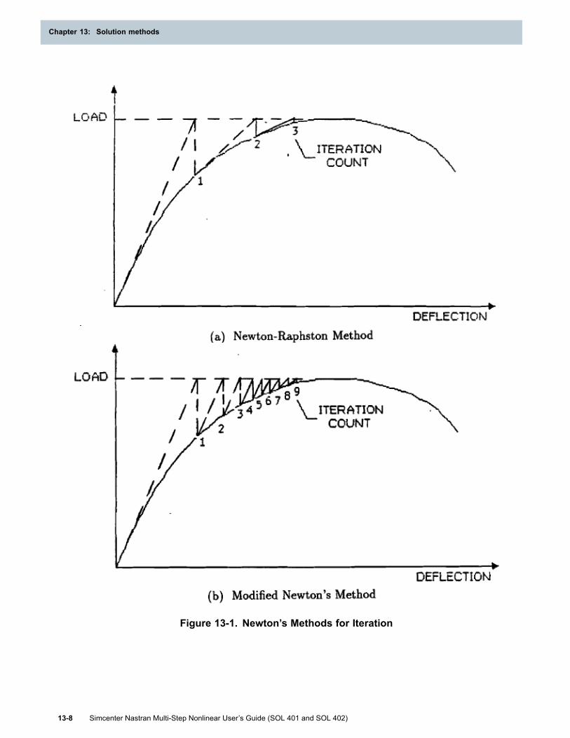
Chapter 13: Solution methods
Figure 13-1. Newton’s Methods for Iteration
13-8 Simcenter Nastran Multi-Step Nonlinear User’s Guide (SOL 401 and SOL 402)
Chapter 13: Solution methods

Solution methods
13.6 Stiffness update strategiesAmong other features of the solution algorithm, the stiffness matrix update has probably the mostprofound effect on the success of the nonlinear solution. In spite of its significance, however, it isvery difficult to implement a robust algorithm for update strategy due to the lack of a prior informationregarding the right timing for an update. In this section, stiffness update strategies are reviewed withrespect to the static analysis. Variations of the modified Newton’s method are adopted in the software.
However, the modified Newton’s method could lead to divergence when the stiffness changesdrastically, as demonstrated in the figure Newton’s Methods for Iteration, unless the tangentialstiffness is reevaluated at the critical point. To this end, an adaptive matrix update method isunavoidable. Stiffness update strategies are established to update the stiffness matrix on an asneeded bases such as probable divergence.
13.6.1 Update principles
Newton’s method could be trapped in an infinite loop, oscillating about the local maximum asillustrated in the figure Newton’s Methods for Iteration (a). This difficulty is overcome during theNewton’s iteration by discarding the differential stiffness, [Kd], when the tangential stiffness is notpositive definite as shown in (b) of that figure.
Control over the stiffness update method is achieved with the KUPDATE parameter on the NLCNTLentry:
1. If KUPDATE=1 (Full Newton method), stiffness is updated after each iteration.
2. If KUPDATE=0 (Auto method, default), stiffness is updated based on the change in the valueof current stiffness parameter since the last stiffness update.
3. If KUPDATE=-1 (Initial stiffness method), no stiffness update is made during the solution.
4. If KUPDATE=N (N>1,Quasi Newton method), if solution time step doesn’t converge in Niterations, stiffness is updated at the iterated configuration. If the parameter TSTEPK is setto YES (Default=NO) on the NLCNTL entry, then stiffness update is also performed beforebeginning a new time step.
Current stiffness parameter approach for the automatic stiffness update method (KUPDATE=0)
The current stiffness parameter approach proposed by Bergan and Crisfield [*] is used for automaticstiffness update method. The current stiffness parameter gives a scalar measure for the stiffness ofthe structure at the current loading condition.
Where, n is the time step index,
I is the teration index,
∆Pni = Pni-Pn-1i is the incremental applied load between time step n-1 and n,
∆P11 = P11 - P01 is the initial applied load (for the first iteration of the first time step),
P11 is the applied load in the first iteration of the first time step of the first subcase,
Simcenter Nastran Multi-Step Nonlinear User’s Guide (SOL 401 and SOL 402) 13-9
Solution methods

Chapter 13: Solution methods
∆Uni = Uni - Un-1i is the incremental displacement between time step n-1 and n,
∆U11 = U11U01 is the initial displacement increment (after the first iteration of first step).
After the first iteration of the first step, S11=1, that is, the initial value of the current stiffness parameteris one. After each iteration, the value of current stiffness parameter is recomputed. The change incurrent stiffness parameter is computed for each iteration as:
Where, Sref is the reference value for current stiffness parameter. At the start of the solution, Sref isset to 1.0. Stiffness is updated if ∆S≥α, where α=5.0 for a problem with structural loading only, α=20.0for a problem with pure thermal load, and α=10.0 for a problem with a combination of structural andthermal load. The value for α can be defined by the user on the NLCNTL card through parameterCSTFPAR. Valid input for CSTFPAR is a real number.
Sref is updated upon updating stiffness to correspond to the value of Sni.
1. Bergan. P, Horrigmoe. G, Krakeland . B, and Soreide T., SOLUTION TECHNIQUES FORNON-LINEAR FINITE ELEMENT PROBLEMS, International Journal for Numerical Methodsin Engineering, Vol. 12, 1677-1696 (1978)
2. Crisfield M. A. , Non-linear Finite Element Analysis of Solids and Structures, Volume 1:Essentials, John Wiley & Sons, Chichester, 1991
13.6.2 Divergence criteria
The MAXDIV parameter in the NLCNTL entry requires an integer to specify a limit on the probabledivergence conditions allowed for each time step to continue. In each iteration of a time step, thefollowing three quantities are computed:
Equation 13-9.
Equation 13-10.
Equation 13-11.
where,
Rni-1=Pni-1-Fni-1 (Uni-2) is the residual for iteration i-1 for time step n,
13-10 Simcenter Nastran Multi-Step Nonlinear User’s Guide (SOL 401 and SOL 402)
Chapter 13: Solution methods

Solution methods
ΔUni=K-1 Rni-1 is the displacement increment computed in iteration i-1 for time step n,
Rni=Pni-Fni (Uni-1) is the residual for iteration i for time step n,
εpi is the computed error for the force norm for iteration i for time step n,
εpi-1 is the computed error for the force norm for iteration i-1 for time step n,
εwi is the computed error for the energy norm for iteration i for time step n,
εwi-1 is the computed error for the energy norm for iteration i-1 for time step n.
For the first iteration of every new time step, the value for λpi and λwi is set to 0.9999. The variableNDIV is initiated to 0 in the first iteration of each time step. NDIV is incremented if:
1. If Er>1 or Er<-100, NDIV=NDIV+1
2. If λwi>1.00 and λpi>1.00, NDIV=NDIV+1
NDIV is reset to 0 if neither of the two conditions above are met in any given iteration. The solutionis considered to have diverged if NDIV>MAXDIV. MAXDIV is a NLCNTL parameter which controlsmaximum allowable divergences in a time step (Default=3).
Upon divergence, the software will:
1. Revert the solution to the last converged point.
2. Reform stiffness at the last converged configuration (unless KUPDATE=-1, in that case nostiffness update is performed).
3. Perform bisection, and attempt to solve the time step with a reduced size from the last convergedpoint.
For a timestep of size Δt, on bisection the time step is reduced to:
Δt1=1/2 Δt
Bisection continues until the solution converges, that is,
Δtk = 1/2 Δtk-1 = 1/2k Δt
where k is a bisection count. Once the bisection is successful (rendering a converged solution),the integration proceeds to the next time step. If k = 1, the same time step size is used for thenext time step.
If k > 1, an effort is made to accelerate the solution process by increasing the time step size forthe next step. The time step size for the next time step is influenced by all of the following factors:
a. The number of iterations (i) that were required to reach convergence with time step size of Δtk.
b. Number of bisections (k) performed.
c. Remaining time left (δt) to complete the original time step of size Δt.
The time step size used for the next time step is m Δtk, where 1 ≤ m ≤ k – 1. The largestvalue of m that satisfied the following conditions is used:
A. I ≤ 3 or I ≤ MAXITR/2m, where MAXITR is the maximum permissible iterations for a giventimestep.
Simcenter Nastran Multi-Step Nonlinear User’s Guide (SOL 401 and SOL 402) 13-11
Solution methods

Chapter 13: Solution methods
B. δt/m Δtk is an integer greater than 0.
Although the goal of increasing time step size is to reduce the number of time steps tillcompletion of solution, for some problems, further bisection may be required in subsequentsteps.
The maximum number of bisections is limited by the parameter MAXBIS (default=5). Thebisection process is activated on an as-needed basis. You also have an option to suppressbisection by specifying MAXBIS=0.
d. If the solution fails to converge even after attempting maximum permissible bisections, thesolution is terminated with a fatal message. Results corresponding to the last converged userrequested output time are printed.
13.7 Convergence criteriaThe convergence test is an important factor that affects accuracy and overall efficiency in nonlinearfinite element analysis. Out-of-balance forces and changes in displacements should vanish uponconvergence in an iterative process. The energy error accommodates both quantities and is usuallyadequate for most problems. However, the displacements could be in gross error while the residualload error is negligible, or vice versa.
In order to ensure accurate and consistent convergence, multiple criteria with errors measured interms of displacements, loads, and energy should be combined. It is the error function and theconvergence tolerance that characterize the criteria. Error functions are formulated using theweighted normalization so that the error measures are dimensionless. Tolerances should be realisticfor the solution scheme to be efficient. In this context, variations are considered in search of the bestworkable combinations of error functions and tolerances for a wide class of structural problems.
13.7.1 Rudimentary considerations
The convergence test is a decision-making process, on which termination of the iterative process isbased, while the true solution is not known. The convergence criteria are extremely important for theincremental/iterative solution strategy to be effective and efficient, because improper criteria couldcause inefficiency as well as inaccuracy. It is rather astounding to:find a scarcity of publications onthis subject, considering the significant impact of the convergence criteria on the accuracy and theefficiency of the computation. Two distinct aspects are involved in the convergence criteria:
• Error functions to be minimized by the iteration.
• Tolerances of error functions within which errors are acceptable.
Both aspects must be defined properly for the criteria to be effective, for the solution scheme tobe efficient, and for the solution to be accurate.
There are no universally accepted convergence criteria to date in the field of finite element analysis.Conditions to be met by ideal convergence criteria for a general-purpose finite element analysis havebeen contemplated. The convergence criteria should:
• be satisfied for linear cases at all times.
• be independent of structural units.
13-12 Simcenter Nastran Multi-Step Nonlinear User’s Guide (SOL 401 and SOL 402)
Chapter 13: Solution methods

Solution methods
• be reliable (cancellation of errors are not acceptable).
• render consistent accuracy.
• be independent of structural characteristics (stiffening or softening).
• be able to handle all the loading cases including constant loading, unloading, and no externalloading (applicable to creep analysis).
• have smooth transitions after the stiffness updates and loading changes.
These conditions dictate the formulation of error functions to be discussed.
13.7.2 Convergence conditions
The iteration continues until the convergence is attained by satisfying the convergence criteria andthe residual error vector at convergence is carried over to the next incremental step. When theconvergence criteria are satisfied, the out-of-balance forces and the changes in displacements shouldbe sufficiently small so that the remaining error is not physically significant nor will it cause anydetrimental effects, numerically or physically, on the succeeding incremental steps. Convergencetolerances have the following effects:
• excessively tight tolerances cause a waste of computing resources for unnecessary accuracy.
• excessively loose tolerances cause not only inaccuracy but convergence difficulties in thesubsequent steps due to cumulative errors.
The fundamental difficulty of the convergence tests for a structural analysis lies in the fact thatthe base vectors (forces and displacements) involve inconsistent units, namely, combinations offorces and moments or translations and rotations. Indiscriminate use of these vectors will causeunit-dependent convergence criteria. For example, while an error in forces is dominant when themodel is expressed in newton-meter, the error would be dominated by moments if the same model isdescribed in newton-millimeter.
The most natural and reasonable criterion for the convergence test is formulated in terms of anenergy error. The energy error is the logical choice because both the out-of-balance forces {R}and the change in displacements {Δu} should be minimized by the iteration process. Furthermore,energy quantities do not pose problems of inconsistent units due to mixed units associated withtranslations and rotations.
Although the convergence test in terms of energy errors is usually adequate, some distinct errorsare not detected with this criterion; i.e., displacements are in gross error while the residual loaderror is negligible, or vice versa. This would be the case if the degrees-of-freedom in error have avery small or a very large stiffness. Such cases compel the need for criteria in terms of loads anddisplacements. Nominally, by visualizing the load-deflection curve for a one-dimensional case, it canbe noticed that the convergence criterion in terms of loads governs the stiffening structure and thecriterion in terms of displacements governs the softening structure. Scalar error functions for thesecriteria are formulated to be dimensionless by introducing the weighted normalization.
Simcenter Nastran Multi-Step Nonlinear User’s Guide (SOL 401 and SOL 402) 13-13
Solution methods

Chapter 13: Solution methods
13.7.3 SOL 401 Error functions and weighted normalization
A nonlinear solution iterates until the software computed convergence error functions are lessthan the convergence criteria you have defined for each function. A convergence error function iscalculated with a ratio which compares the value of displacement, force, or work for the currentincrement to the total value of displacement, force, or work. Error in energy (work) is used as thedefault convergence criterion. These criteria are computed as follows.
For the displacement and residual force error criterion, you can use the NORMP and NORMUparameters on the NLCNTL bulk entry to select the vector norm. In general, the norm computationresults in a strictly positive value from a vector space νn such that:
• The displacement convergence error function with the norm criteria is as follows.
where,
Uni is the displacement vector for iteration i of time step n,
Uni-1 is the displacement vector for iteration i-1 of time step n, and
Un-1 is the displacement vector at convergence for time step n-1.
Optionally, when the REFU parameter is defined, the form of the displacement error function isas follows.
• The force convergence error function with the norm criteria is as follows.
where,
Pni is the external force vector for iteration i of time step n,
Fni is the internal force vector for iteration i of time step n,
Rni is the residual force vector for iteration i of time step n, and
Rn1 is the residual force vector for iteration 1 of time step n.
Optionally, when the REFP parameter is defined, the form of the force error function is as follows.
13-14 Simcenter Nastran Multi-Step Nonlinear User’s Guide (SOL 401 and SOL 402)
Chapter 13: Solution methods

Solution methods
• EPSW (work criterion)
Equation 13-12.
Where,
ΔUniis the incremental displacement vector computed for iteration i of time step n,
Rni is the residual force vector for iteration i of time step n,
Uni is the total displacement vector for iteration i of time step n,
Pni is the external force vector for iteration i of time step n,
Fni is the internal force vector for iteration i of time step n,
Rn1 is the residual force vector for iteration 1 of time step n, and
Un1 is the total displacement vector for iteration 1 of time step n.
Default tolerances for these error criteria are:
EPSU (Displacement): 1.0E-2
EPSP (Force): 1.0E-2
EPSW (Work): 1.0E-6
You can specify custom convergence tolerances on the NLCNTL bulk entry. The solution isconsidered to have converged if the computed error criteria are less than the tolerance specified.
13.7.4 SOL 402 Error functions and weighted normalization
A nonlinear solution iterates until the software computed convergence error functions are lessthan the convergence criteria you have defined for each function. A convergence error function iscalculated with a ratio which compares the value of displacements, forces (or contact forces), or workfor the current increment to the total value of displacements, forces, or work.
Although all criteria theoretically need to be satisfied, force is practically used as the principalconvergence criterion. These criteria are computed as follows.
In general, the norm computation results in a strictly positive value from a vector space xn such that:
The displacement convergence error function with the norm criterion is as follows.
Simcenter Nastran Multi-Step Nonlinear User’s Guide (SOL 401 and SOL 402) 13-15
Solution methods

Chapter 13: Solution methods
where,
is the incremental displacement vector computed for iteration i of time step n,
is the displacement vector for iteration i of time step n,
is the displacement vector for iteration i-1 of time step n.
Optionally, when the REFU parameter is defined, the form of the displacement error function isas follows.
The force convergence error function with the norm criterion is as follows.
where,
is the external force vector for iteration i of time step n,
is the internal force (including the inertial force if it exists) vector for iteration i of time step n,
is the residual force vector for iteration i of time step n.
Optionally, when the REFP parameter is defined, the form of the force error function is as follows.
The energy convergence error function is as follows.
is the incremental displacement vector computed for iteration i of time step n,
is the residual force vector for iteration i of time step n,
13-16 Simcenter Nastran Multi-Step Nonlinear User’s Guide (SOL 401 and SOL 402)
Chapter 13: Solution methods

Solution methods
is the work by the external force for iteration i of time step n,
is the work by the internal force (including the inertial force if it exists) for iteration i of timestep n.
Note that the work at the time step n also relates to the work at the precedent time step n-1, that is.:
where,
is the work by the external force at convergence for time step n-1,
is the work by the internal force (including the inertial force if it exists) at convergencefor time step n-1,
is the displacement vector at convergence for time step n-1,
is the external force vector at convergence for time step n-1,
is the internal force (including the inertial force if it exists) vector at convergence for timestep n-1,
is the displacement vector for iteration i of time step n,
is the external force vector for iteration i of time step n,
is the internal force (including the inertial force if it exists) vector for iteration i of time step n.
Optionally, when the REFE parameter is defined, the form of the force error function is as follows.
The contact force convergence error function with the norm criteria is as follows.
is the incremental contact force vector computed for iteration i of time step n,
Simcenter Nastran Multi-Step Nonlinear User’s Guide (SOL 401 and SOL 402) 13-17
Solution methods

Chapter 13: Solution methods
is the contact force vector for iteration i of time step n,
is the contact force vector for iteration i-1 of time step n.
Optionally, when the REFP parameter is defined, the form of the contact force error function isas follows.
Default tolerances for these error criteria are:
PRCQ (Displacement): 1.0E-1
PRCR (Force): 1.0E-3
PRCE (Work): 1.0E-3
PRCF (Contact Force): 1.0E-1
You can specify custom convergence tolerances on the NLCNTL2 bulk entry. The solution isconsidered to have converged if the computed error criteria are less than the tolerance specified.
13.7.5 Implementation
The convergence tolerance determines the efficiency of the solution scheme as well as the accuracyof the solution. The tolerance should be realistic, not too tight nor too loose. It is difficult to chooseoptimal default values for the convergence tolerances. However, efforts have been made to set thedefault values to provide reliable solutions to the general class of problems. Thus, default tolerancesshould be adhered to until good reasons are found to change them.
SOL 401 error functionsThe following three error functions (in terms of displacements, loads, and energy) are computedand compared to tolerances.
Eu < EPSU (=10-2 by default)
Ep < EPSP (=10-2 by default)
Ew < EPSW (=10-6 by default)
where EPSU, EPSP, and EPSW are tolerances specified in the NLCNTL entry. However, onlythose criteria chosen by the user (combinations of U,P, and/or W) are designed to be satisfied forconvergence.
It is noted that divergence conditions are established independent of convergence criteria.
SOL 402 error functionsThe following error functions (in terms of displacements, loads, and energy) are computed andcompared to tolerances.
Eu < PRCQ (=10-1 by default)
Ep < PRCR (=10-3 by default)
Ew < PRCE (=10-3 by default)
13-18 Simcenter Nastran Multi-Step Nonlinear User’s Guide (SOL 401 and SOL 402)
Chapter 13: Solution methods

Solution methods
Ec < PRCF (=10-1 by default)
where PRCQ, PRCR, PRCE, and PRCF are tolerances specified in the NLCNTL2 entry.
It is noted that divergence conditions are established independent of convergence criteria.
Simcenter Nastran Multi-Step Nonlinear User’s Guide (SOL 401 and SOL 402) 13-19
Solution methods

Siemens Industry Software
HeadquartersGranite Park One5800 Granite ParkwaySuite 600Plano, TX 75024USA+1 972 987 3000
AmericasGranite Park One5800 Granite ParkwaySuite 600Plano, TX 75024USA+1 314 264 8499
EuropeStephenson HouseSir William Siemens SquareFrimley, CamberleySurrey, GU16 8QD+44 (0) 1276 413200
Asia-PacificSuites 4301-4302, 43/FAIA Kowloon Tower, Landmark East100 How Ming StreetKwun Tong, KowloonHong Kong+852 2230 3308
About Siemens Digital Industries Software
Siemens Digital Industries Software is drivingtransformation to enable a digital enterprise whereengineering, manufacturing, and electronics design meettomorrow. Our solutions help companies of all sizes createand leverage digital twins that provide organizations withnew insights, opportunities, and levels of automationto drive innovation. For more information on SiemensDigital Industries Software products and services, visitsiemens.com/software or follow us on LinkedIn, Twitter,Facebook, and Instagram.
Siemens Digital Industries Software —Where today meets tomorrow.
© 2019 Siemens. A list of relevant trademarks canbe found here. All other trademarks belong to theirrespective owners.


