The Pennsylvania State University

The Graduate School

Harold and Inge Marcus

Department of Industrial and Manufacturing Engineering

MULTI-STAGE STOCHASTIC PROGRAMMING ON

SHALE GAS INFRASTRUCTURE AND PRODUCTION PLANNING

A Thesis in

Industrial Engineering and Operations Research

by

Xiaohuang Wu

2012 Xiaohuang Wu

Submitted in Partial Fulfillment

of the Requirements

for the Degree of

Master of Science

August 2012

The thesis of Xiaohuang Wu was reviewed and approved* by the following:

Tao Yao

Associate Professor of Industrial and Manufacturing Engineering

Thesis Advisor

Jack C. Hayya

Professor Emeritus of Management Science and Information Systems

Paul Griffin

Professor of Industrial and Manufacturing Engineering

Peter and Angela Dal Pezzo Department Head Chair

*Signatures are on file in the Graduate School

iii

ABSTRACT

The rich resource of Marcellus gas has recently boosted up the interest of people

as the drilling technology advances. Apart from the difficulties in exploration and drilling

for natural gas, problems of building and developing network that delivers the gas to

customers remain unsolved for shale gas companies and government. In the paper, we

investigate an in-land shale gas infrastructure and production planning problem. Multiple

gas fields with uncertain reserves are considered. Platforms are connected by pipelines,

which will eventually transport the gas to a central pipeline that delivers gas to merchants

and customers. The goal is to obtain the maximum expected net present value of the

project within a given time horizon. As the revelation of field reserves will affect the

decision maker’s action, we develop a stochastic model with endogenous uncertainties.

Modern stochastic programming technique is applied. Specifically, conservative

approximations are obtained under the assumption of piecewise constant binary and

linear real-valued decision rules. The decision rule approximation successfully solves a

small sized example with continuously distributed uncertainty parameters. Near-optimal

results are obtained efficiently and can be improved by increasing partition subsets.

iv

TABLE OF CONTENTS

List of Figures .............................................................................................................. v

List of Tables ............................................................................................................... vi

Acknowledgements ...................................................................................................... vii

Chapter 1 Introduction ................................................................................................. 1

Chapter 2 Literature Review ........................................................................................ 4

Chapter 3 Problem Statement ...................................................................................... 7

Chapter 4 One-stage Infrastructure and Production Planning ..................................... 12

Model .................................................................................................................... 12 Approximation ...................................................................................................... 13 Numerical Example .............................................................................................. 15

Chapter 5 Multi-stage Infrastructure and Production Planning ................................... 21

Model .................................................................................................................... 21 Approximation ...................................................................................................... 22 Numerical Example .............................................................................................. 26

Chapter 6 Conclusions and Future Work ..................................................................... 40

List of References ........................................................................................................ 41

v

List of Figures

Figure 3-1. Shale gas network. .................................................................................... 7

vi

List of Tables

Table 3-1. Notation. ..................................................................................................... 8

Table 4-1. Input parameters for one-stage. .................................................................. 16

Table 5-1. Input parameters for multi-stage. ............................................................... 28

Table 5-2. Partition of uncertainty set. ......................................................................... 31

Table 5-3. Optimal construction. ................................................................................. 34

Table 5-4. Optimal gas extraction. ............................................................................... 35

Table 5-5. Optimal capacity expansion. ...................................................................... 36

Table 5-6. Optimal gas flow. ....................................................................................... 37

vii

Acknowledgements

First, I want to thank my thesis advisor, Dr. Yao. It is his guidance, insights and

patience that make it possible for me to rise in the academic world, one full of joy and

surprise that I have never experienced before. I also want to thank my thesis reader Dr.

Hayya and department chair Dr. Griffin for spending their time reading my thesis and

providing me with valuable feedback. Finally, I want to thank my family and my friends.

Without their persistent support, I could not have made it this far. They are and will

always be the most important part of my life.

Chapter 1

Introduction

The Marcellus shale, a layer of shale rock beneath the rolling hills and mountains

of Pennsylvania, is the largest unconventional natural gas reserve in the world. This well-

known geological formation that contains significant amounts of natural gas was never

considered worthwhile until recent technology advances. Though reserve estimates are

considered uncertain at this point, most of the completed Marcellus well revealed

abundant recoverable reserves. Together with the emphasis on consuming green energy

due to environmental issues, natural gas, which has considerably lower carbon content

than petroleum and coal, will no doubt grasp its own share of the market.

Marcellus shale gas play becomes more and more attractive these days as the

drilling technology advances. Reports show that the activity in the Marcellus will

continue to expand and natural gas production from Marcellus could rise to almost 4

billion cubic feet BCF per day by 2020 (Considine and Watson 2009). However, among

some key factors affecting development is infrastructure and production planning.

Though it may seem hard to explore and drill for natural gas, the real work happens to be

the development of a network consisting of thousands of miles of gathering lines and

pipelines to carry the gas to consumers (Considine et al. 2010). Besides, building natural

gas processing facilities takes considerable time and incurs significant costs. To sum up,

developing transportation and production processing networks takes money and time. But

the high potential environment and investment impact stimulates the research.

2

One of the most major concerns is that the decision maker is exposed to a great

deal of uncertainty. Though the location of gas fields could be identified, the amount of

gas in these reserves remains uncertain until the platform is built. Therefore, it is crucial

to take uncertainties into account when formulating the model.

A typical shale gas infrastructure and production problem has multiple potential

reserves within a region to build well platforms on. The extracted natural gas needed to

be purged and dried before sold to merchants and customers for use. Therefore, a

production platform is usually built on site to process the gas before it can be transported

to other areas. In the paper, we call the combo of well platform and production platform

‘a platform’ in general. After the gas is processed on site, it is transported via pipelines

that connecting platforms together. All the gas produced is to be transported to a central

pipeline that connects different regions together. The shale gas infrastructure and

production planning problem requires the decision maker to select when and where to

build platforms, to increase the capacity of platforms and to install pipelines. Besides,

operation decisions are to be made to determine the production schedule for different gas

fields.

For simplification, the planning horizon is discretized into time periods. The

decision maker is to make decision at the beginning of each time period and all the

decision take immediate effect. As the decisions regarding when and where to build

platforms and pipelines are represented as binary variables, and other decisions including

the capacity expansion and extraction schedule are real-valued, the formulation has the

form of mixed binary integer programming. However, all the decision variables are

dependent on the information of gas reserves. The problem thus becomes a stochastic

3

programming with endogenous uncertainties. In the following chapter, we will present

both a one-stage and a multi-stage stochastic programming model for the shale gas

infrastructure and production planning.

The paper is organized as follows:

In chapter 2, a literature review is presented regarding previous work on gas

production planning. Research works on stochastic programming that are used to handle

uncertainty are also summarized.

In chapter 3, the problem statement and assumptions are presented. The

description of the model is also discussed.

In chapter 4 and 5, models are built for the one-stage and the multi-stage

infrastructure and production planning respectively. An approximation of each one of the

problems is presented followed by a numerical example with three gas fields and five

links.

The last chapter consists of conclusions of the thesis together with some

suggested future research directions.

Chapter 2

Literature Review

The economic impact of shale gas is studied by Considine et al. (2009, 2010).

They use IMPLAN modeling system to estimate the job creation, value added, etc.

However, the development of the shale gas network consisting of thousands of miles of

gathering lines and pipelines to carry the gas to consumers remains a major concern

(Considine et al. 2010).

Though the shale gas infrastructure and production planning problem is a

relatively new topic, there have been intensive research studies regarding the oil and gas

field infrastructures. Comprehensive studies on deterministic approaches can be dated

back to 1998 (Ierapetritou, Floudas, Vasantharajan and Cullick, 1998; Iyer, Grossmann,

Vasantharaja and Cullick, 1998; Grothey and McKinnon, 2000; Barnes, Linke and

Kokossis, 2002; Kosmidis, Perkins and Pistikopoulos, 2002; Lin and Floudas, 2003;

Ortiz-Gomez, Rico-Ramirez and Hernandez-Castro, 2002). Uncertainty has also been

considered in some of the literatures (Haugen 1996; Meister, Clark and Shah 1996;

Jonsbraten 1998; Goel and Grossmann 2004).

A dynamic stochastic programming model that incorporates with uncertainty in

the size of oil fields is proposed by Haugen (1996). The author only considers the

decisions made for scheduling of oil fields. Exploration and production decisions for one

field under uncertainty in reserves and oil price are studied by Meister, Clark and Shah

(1996). Jonsbraten (1998) uses the progressive hedging algorithm to make decisions for

5

an oil field with uncertainty in oil prices. The problem is formulated as a mixed integer

linear programming. The author also studies the sequencing of oil wells under uncertainty

in size of oil fields. Both of these two works only include one oil field.

Based on the dependence of the order of revelation of uncertainties on decision

maker’s action in stochastic programming, the uncertainties can be categorized as

exogenous uncertainties and endogenous uncertainties (Jonsbraten 1998). Jonsbraten

(1998) investigates decision problems in which actions can affect both the distribution of

the uncertainties and the timing of revelation. Besides, there are research studies focusing

on problems based on the assumption that uncertain parameters follow a discrete

distribution, which could be solved using a finite scenario tree. Goel and Grossmann

(2004) propose a model for off-shore gas field development problem with discretely

distributed endogenous uncertainties and reformulate it as a mixed binary program.

Problems with continuously distributed random parameters, otherwise, need to be

discretized before any of the above techniques can be applied. One alternate solution

could be Monte Carlo sampling, but such technique is not considered computationally

efficient (Dyer and Stougie 2006, Shapiro and Nemirovski 2005). While discretization

may be able to get accurate approximations, it can increase computing cost dramatically

when applied to medium or large-sized problems. Vayanos and Kuhn (2011) proposed a

methodology for solving dynamic problems with endogenous uncertainties. They suggest

approximating the adaptive measurement decisions by piecewise constant functions and

the adaptive real-valued decisions by piecewise linear functions of the uncertainties.

The contribution of this paper is as follows:

6

First, in this paper, we seek to propose models suitable for in-land shale gas

infrastructure and production planning, which has not been studied before. A one-stage

model and a multi-stage model with endogenous uncertainties are presented respectively.

The assumptions and restrictions of the model are discussed.

Second, most of the past research works in oil field development planning under

uncertainty deal with discretely distributed random parameters or a single oil field. We

explore the problem in a broader context as multiple oil fields with continuously

distributed uncertain reserves are presented and the project can last for multiple time

horizons.

Finally, we provide a stochastic programming technique to solve the multi-region

and multi-stage dynamic decision making problem efficiently by partition of uncertainty

set. Near-optimal conservative approximations are obtained under the assumption of

piecewise constant binary and linear real-valued decision rules.

Chapter 3

Problem Statement

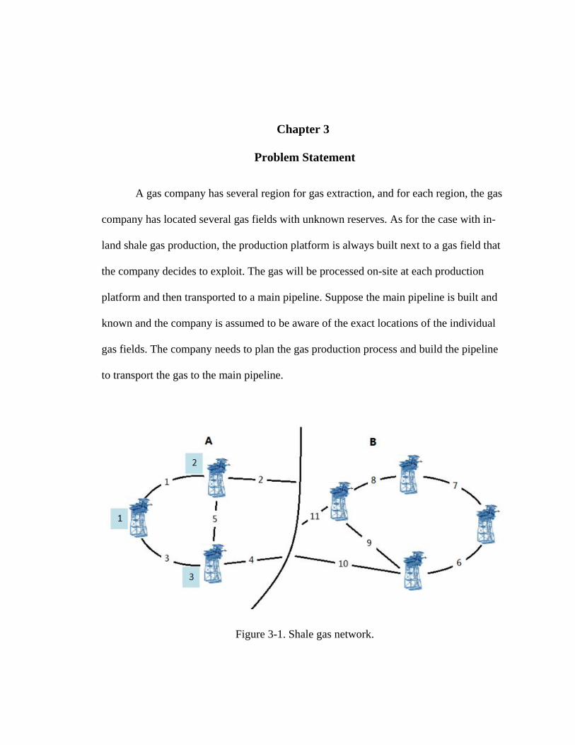
A gas company has several region for gas extraction, and for each region, the gas

company has located several gas fields with unknown reserves. As for the case with in-

land shale gas production, the production platform is always built next to a gas field that

the company decides to exploit. The gas will be processed on-site at each production

platform and then transported to a main pipeline. Suppose the main pipeline is built and

known and the company is assumed to be aware of the exact locations of the individual

gas fields. The company needs to plan the gas production process and build the pipeline

to transport the gas to the main pipeline.

Figure 3-1. Shale gas network.

8

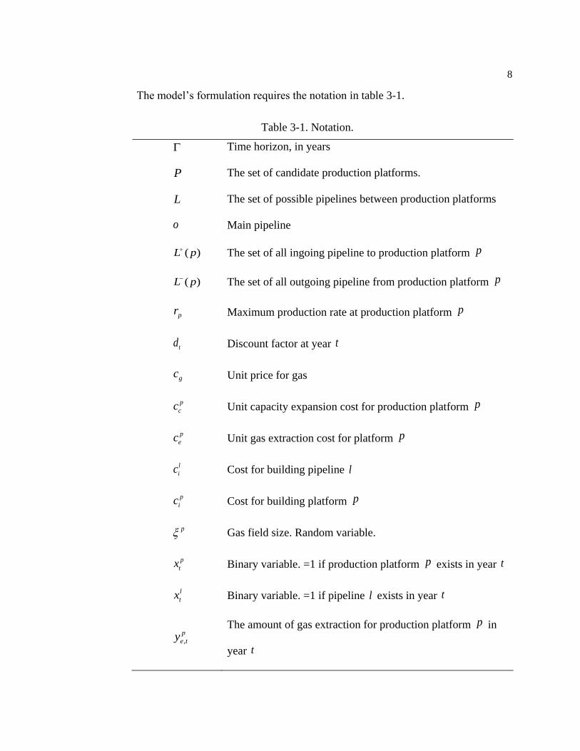
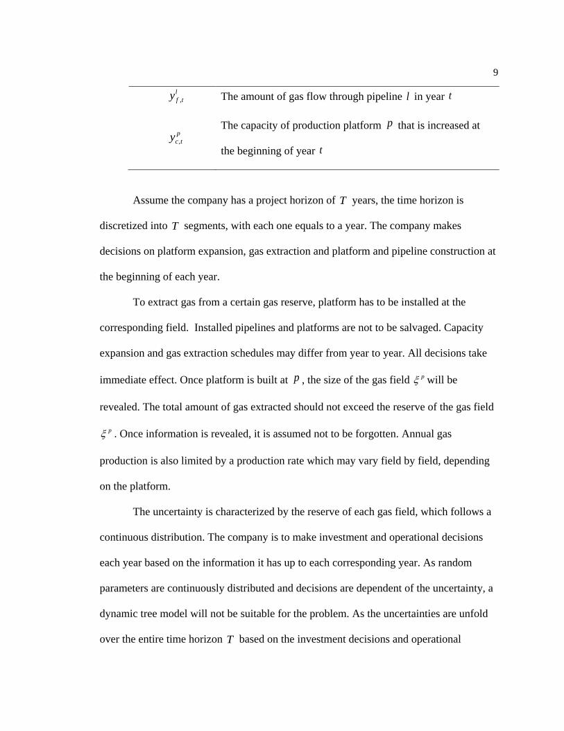
The model’s formulation requires the notation in table 3-1.

Table 3-1. Notation.

Time horizon, in years

P The set of candidate production platforms.

L The set of possible pipelines between production platforms

o Main pipeline

( )L p The set of all ingoing pipeline to production platform p

( )L p The set of all outgoing pipeline from production platform p

pr Maximum production rate at production platform p

td Discount factor at year t

gc Unit price for gas

p

cc Unit capacity expansion cost for production platform p

p

ec Unit gas extraction cost for platform p

l

ic Cost for building pipeline l

p

ic Cost for building platform p

p Gas field size. Random variable.

p

tx Binary variable. =1 if production platform p exists in year t

l

tx Binary variable. =1 if pipeline l exists in year t

,

p

e ty

The amount of gas extraction for production platform p in

year t

9

,

l

f ty The amount of gas flow through pipeline l in year t

,

p

c ty

The capacity of production platform p that is increased at

the beginning of year t

Assume the company has a project horizon of T years, the time horizon is

discretized into T segments, with each one equals to a year. The company makes

decisions on platform expansion, gas extraction and platform and pipeline construction at

the beginning of each year.

To extract gas from a certain gas reserve, platform has to be installed at the

corresponding field. Installed pipelines and platforms are not to be salvaged. Capacity

expansion and gas extraction schedules may differ from year to year. All decisions take

immediate effect. Once platform is built at p , the size of the gas field p will be

revealed. The total amount of gas extracted should not exceed the reserve of the gas field

p . Once information is revealed, it is assumed not to be forgotten. Annual gas

production is also limited by a production rate which may vary field by field, depending

on the platform.

The uncertainty is characterized by the reserve of each gas field, which follows a

continuous distribution. The company is to make investment and operational decisions

each year based on the information it has up to each corresponding year. As random

parameters are continuously distributed and decisions are dependent of the uncertainty, a

dynamic tree model will not be suitable for the problem. As the uncertainties are unfold

over the entire time horizon T based on the investment decisions and operational

10

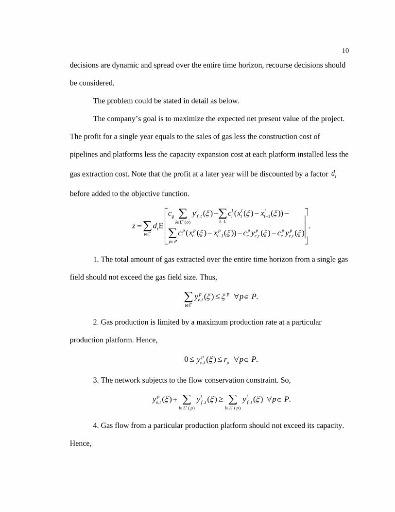
decisions are dynamic and spread over the entire time horizon, recourse decisions should

be considered.

The problem could be stated in detail as below.

The company’s goal is to maximize the expected net present value of the project.

The profit for a single year equals to the sales of gas less the construction cost of

pipelines and platforms less the capacity expansion cost at each platform installed less the

gas extraction cost. Note that the profit at a later year will be discounted by a factor td

before added to the objective function.

, 1

( )

1 , ,

( ) ( ( ) ( ))

.( ( ) ( )) ( ) ( )

l l l l

g f t i t t

l Ll L o

t p p p p p p pt i t t c c t e e t

p P

c y c x x

z dc x x c y c y

1. The total amount of gas extracted over the entire time horizon from a single gas

field should not exceed the gas field size. Thus,

, ( ) .p p

e t

t

y p P

2. Gas production is limited by a maximum production rate at a particular

production platform. Hence,

,0 ( ) .p

e t py r p P

3. The network subjects to the flow conservation constraint. So,

, , ,

( ) ( )

( ) ( ) ( ) .p l l

e t f t f t

l L p l L p

y y y p P

4. Gas flow from a particular production platform should not exceed its capacity.

Hence,

11

, ,

1( )

( ) ( ) , .t

l p

f t c

l L p

y y p P t

5. No gas flow from pipeline l if the pipeline has not been built. Thus,

,0 ( ) ( ) , .l l

f t ty Mx l L t

6. No expansion can be constructed if production platform p has not been built.

It follows that

,0 ( ) ( ) , .p p

c t ty Mx p P t

7. Existing pipelines and production platforms are not to disappear in the network.

Thus,

1( ) ( ) , ,p p

t tx x p P t

1( ) ( ) , .l l

t tx x l L t

Chapter 4

One-stage Infrastructure and Production Planning

Model

Notation. In this chapter, uncertainty is modeled by a probability space

( , ( ), )k k that consists of the sample space k and the Borel -algebra ( )k ,

which is the set of events that are assigned probabilities by the probability measure .

Let ,k n denote the space of all measureable functions from k to n . Let ( )E denote

the expectation operator with respect to and x y denote the Hadamard product of two

vectors , nx y .

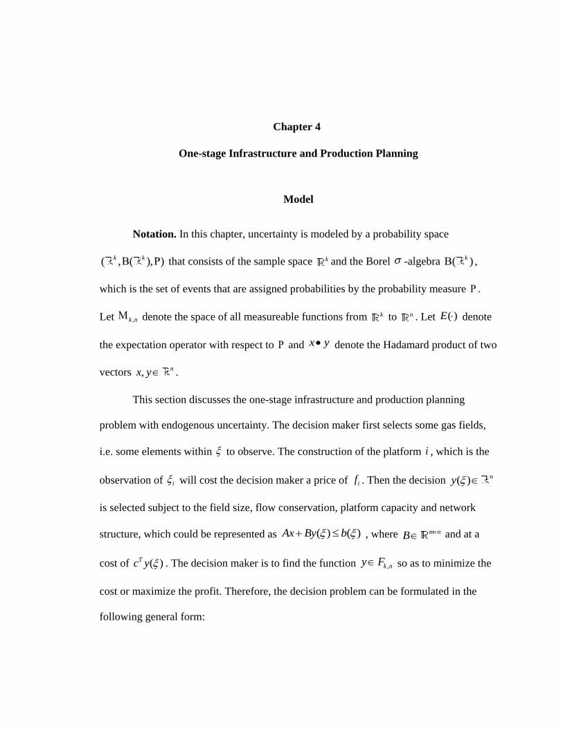
This section discusses the one-stage infrastructure and production planning

problem with endogenous uncertainty. The decision maker first selects some gas fields,

i.e. some elements within to observe. The construction of the platform i , which is the

observation of i will cost the decision maker a price of if . Then the decision ( ) ny

is selected subject to the field size, flow conservation, platform capacity and network

structure, which could be represented as ( ) ( )Ax By b , where m nB and at a

cost of ( )Tc y . The decision maker is to find the function ,k ny F so as to minimize the

cost or maximize the profit. Therefore, the decision problem can be formulated in the

following general form:

13

min ( ( ))T Tf x c y

,. . ,

( ) ( ),

( ) ( )

k

k ns t x y F

Ax d By h

y y x

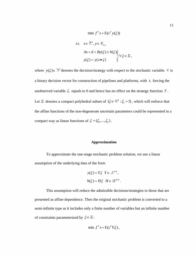
where ( ) ny denotes the decision/strategy with respect to the stochastic variable. x is

a binary decision vector for construction of pipelines and platforms, with ix forcing the

unobserved variable i equals to 0 and hence has no effect on the strategy function y .

Let denotes a compact polyhedral subset of 1{ : 1}k , which will enforce that

the affine functions of the non-degenerate uncertain parameters could be represented in a

compact way as linear functions of 1( ,..., )k .

Approximation

To approximate the one-stage stochastic problem solution, we use a linear

assumption of the underlying data of the form

( ) ,

( ) .

n k

m k

y Y Y

h H H

This assumption will reduce the admissible decisions/strategies to those that are

presented as affine dependence. Then the original stochastic problem is converted to a

semi-infinite type as it includes only a finite number of variables but an infinite number

of constraints parameterized by :

min ( ) ,T Tf x c Y

14

. . ,

.( ) ( )

k n ks t x Y

Ax d BY H

y y x

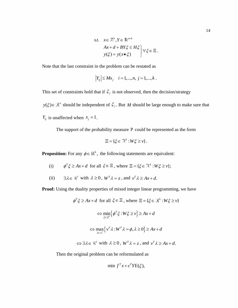
Note that the last constraint in the problem can be restated as

1,..., , 1,..., .ij jY Mx i n j k

This set of constraints hold that if j is not observed, then the decision/strategy

( ) ny should be independent of j . But M should be large enough to make sure that

ijY is unaffected when 1jx .

The support of the probability measure could be represented as the form

{ : }.k W v

Proposition: For any ,k the following statements are equivalent:

(i) T Ax d for all , where { : };k W v

(ii) l with 0 , TW z , and .Tv Ax d

Proof: Using the duality properties of mixed integer linear programming, we have

T Ax d for all , where { : }k W v

min :k

T W v Ax d

max : , 0l

T Tv W Ax d

l with 0 , TW z , and .Tv Ax d

Then the original problem can be reformulated as

min ( ),T Tf x c Y

15

. . , , ,

,

0,

0.

k n k m ls t x Y

W BY H

v Ax d

The above approximation formulation of one-stage stochastic programming can be solved

efficiently as a mixed integer binary program. Its size grows polynomially with , ,k m n

and l , which are the size of the original problem and the number of constraints in the

underlying uncertainty set . The resulting solution is a conservative approximation of

the original problem.

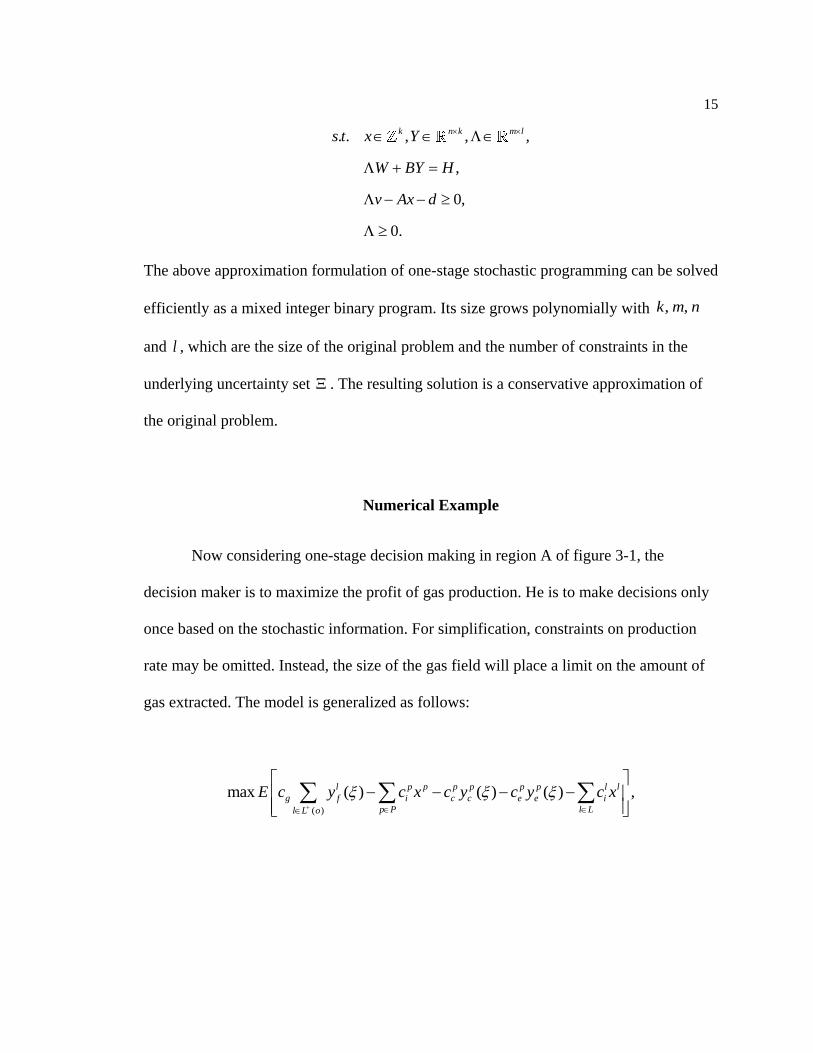
Numerical Example

Now considering one-stage decision making in region A of figure 3-1, the

decision maker is to maximize the profit of gas production. He is to make decisions only

once based on the stochastic information. For simplification, constraints on production

rate may be omitted. Instead, the size of the gas field will place a limit on the amount of

gas extracted. The model is generalized as follows:

( )

max ( ) ( ) ( ) ,l p p p p p p l l

g f i c c e e i

p P l Ll L o

E c y c x c y c y c x

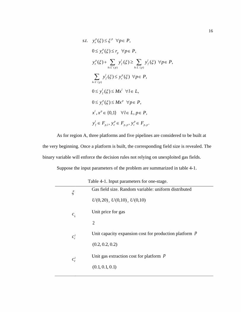
16

( ) ( )

( )

, , ,

. . ( ) ,

0 ( ) ,

( ) ( ) ( ) ,

( ) ( ) ,

0 ( ) ,

0 ( ) ,

, {0,1} , ,

, , .

p p

e

p

e p

p l l

e f f

l L p l L p

l p

f c

l L p

l l

f

p p

c

l p

l p p

f p l e p p c p p

s t y p P

y r p P

y y y p P

y y p P

y Mx l L

y Mx p P

x x l L p P

y F y F y F

As for region A, three platforms and five pipelines are considered to be built at

the very beginning. Once a platform is built, the corresponding field size is revealed. The

binary variable will enforce the decision rules not relying on unexploited gas fields.

Suppose the input parameters of the problem are summarized in table 4-1.

Table 4-1. Input parameters for one-stage.

p

Gas field size. Random variable: uniform distributed

(0,20)U , (0,10)U , (0,10)U

gc

Unit price for gas

2

p

cc

Unit capacity expansion cost for production platform p

(0.2, 0.2, 0.2)

p

ec

Unit gas extraction cost for platform p

(0.1, 0.1, 0.1)

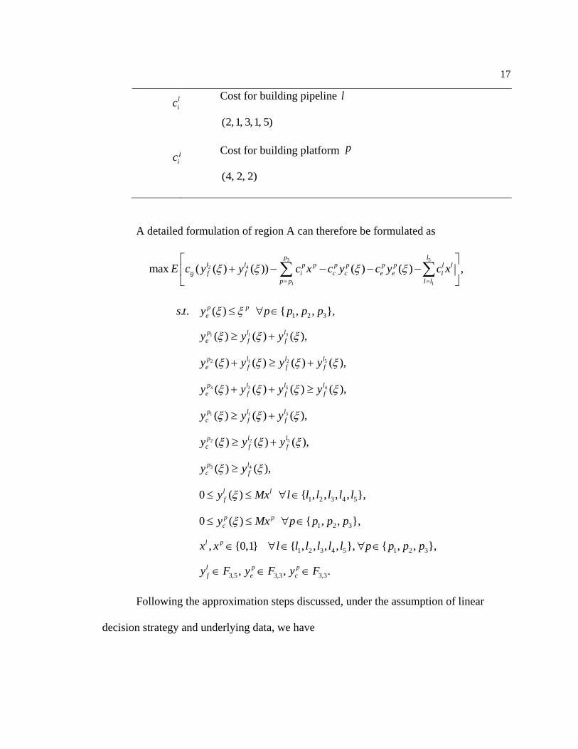
17

l

ic

Cost for building pipeline l

(2,1, 3,1, 5)

p

ic

Cost for building platform p

(4, 2, 2)

A detailed formulation of region A can therefore be formulated as

3 5

2 4

1 1

max ( ( ) ( )) ( ) ( ) ,p l

l l p p p p p p l l

g f f i c c e e i

p p l l

E c y y c x c y c y c x

31 1

52 1 2

3 3 5 4

31 1

52 2

3 4

1 2 3

1 2

. . ( ) { , , },

( ) ( ) ( ),

( ) ( ) ( ) ( ),

( ) ( ) ( ) ( ),

( ) ( ) ( ),

( ) ( ) ( ),

( ) ( ),

0 ( ) { ,

p p

e

lp l

e f f

lp l l

e f f f

p l l l

e f f f

lp l

c f f

lp l

c f f

p l

c f

l l

f

s t y p p p p

y y y

y y y y

y y y y

y y y

y y y

y y

y Mx l l l

3 4 5

1 2 3

1 2 3 4 5 1 2 3

3,5 3,3 3,3

, , , },

0 ( ) { , , },

, {0,1} { , , , , }, { , , },

, , .

p p

c

l p

l p p

f e c

l l l

y Mx p p p p

x x l l l l l l p p p p

y F y F y F

Following the approximation steps discussed, under the assumption of linear

decision strategy and underlying data, we have

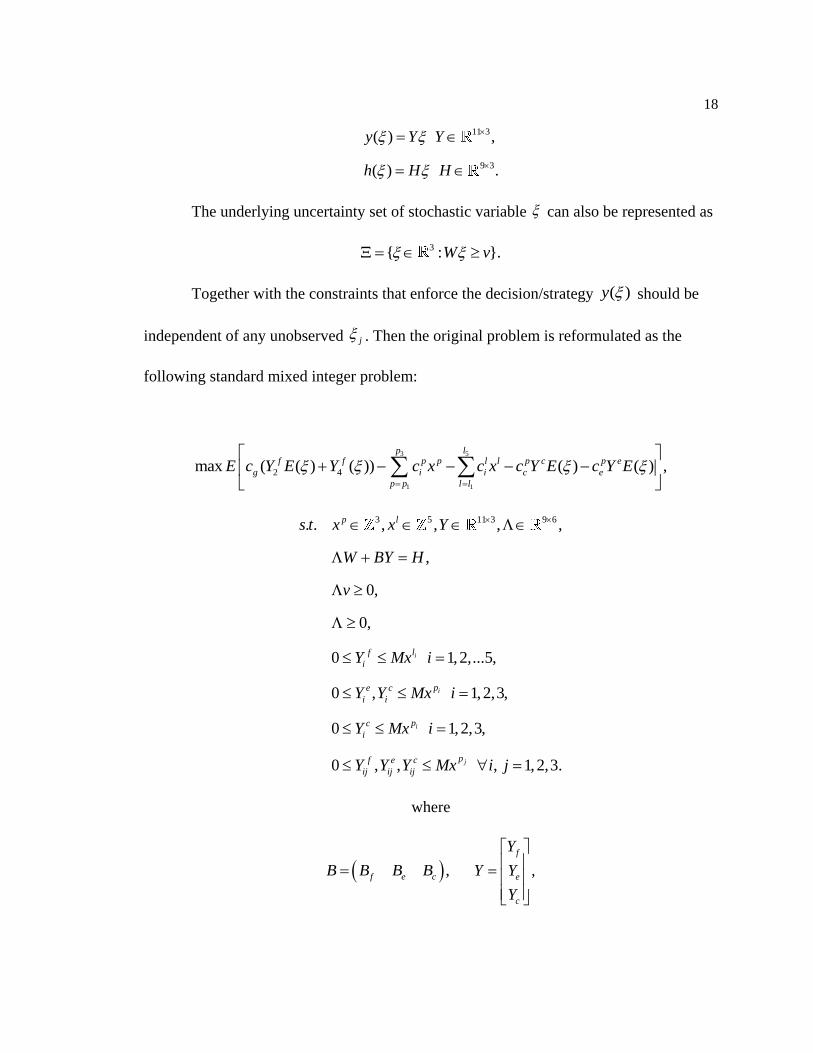
18

11 3

9 3

( ) ,

( ) .

y Y Y

h H H

The underlying uncertainty set of stochastic variable can also be represented as

3{ : }.W v

Together with the constraints that enforce the decision/strategy ( )y should be

independent of any unobserved j . Then the original problem is reformulated as the

following standard mixed integer problem:

3 5

1 1

2 4max ( ( ) ( )) ( ) ( ) ,p l

f f p p l l p c p e

g i i c e

p p l l

E c Y E Y c x c x c Y E c Y E

3 5 11 3 9 6. . , , , ,

,

0,

0,

0 1,2,...5,

0 , 1,2,3,

0 1,2,3,

0 , , , 1, 2,3.

i

i

i

j

p l

lf

i

pe c

i i

pc

i

pf e c

ij ij ij

s t x x Y

W BY H

v

Y Mx i

Y Y Mx i

Y Mx i

Y Y Y Mx i j

where

,f e cB B B B ,

f

e

c

Y

Y Y

Y

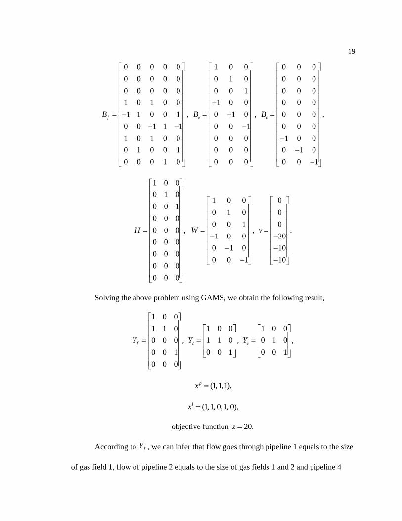
19

0 0 0 0 0

0 0 0 0 0

0 0 0 0 0

1 0 1 0 0

,1 1 0 0 1

0 0 1 1 1

1 0 1 0 0

0 1 0 0 1

0 0 0 1 0

fB

1 0 0

0 1 0

0 0 1

1 0 0

,0 1 0

0 0 1

0 0 0

0 0 0

0 0 0

eB

0 0 0

0 0 0

0 0 0

0 0 0

,0 0 0

0 0 0

1 0 0

0 1 0

0 0 1

cB

1 0 0

0 1 0

0 0 1

0 0 0

,0 0 0

0 0 0

0 0 0

0 0 0

0 0 0

H

1 0 0

0 1 0

0 0 1,

1 0 0

0 1 0

0 0 1

W

0

0

0.

20

10

10

v

Solving the above problem using GAMS, we obtain the following result,

1 0 0

1 1 0

,0 0 0

0 0 1

0 0 0

fY

1 0 0

1 1 0 ,

0 0 1

cY

1 0 0

0 1 0 ,

0 0 1

eY

(1,1,1),px

(1,1, 0,1, 0),lx

objective function 20.z

According to fY , we can infer that flow goes through pipeline 1 equals to the size

of gas field 1, flow of pipeline 2 equals to the size of gas fields 1 and 2 and pipeline 4

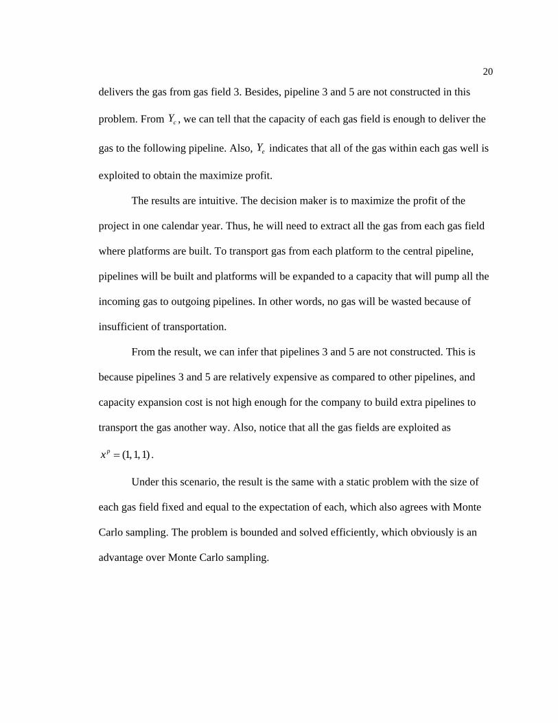
20

delivers the gas from gas field 3. Besides, pipeline 3 and 5 are not constructed in this

problem. From cY , we can tell that the capacity of each gas field is enough to deliver the

gas to the following pipeline. Also, eY indicates that all of the gas within each gas well is

exploited to obtain the maximize profit.

The results are intuitive. The decision maker is to maximize the profit of the

project in one calendar year. Thus, he will need to extract all the gas from each gas field

where platforms are built. To transport gas from each platform to the central pipeline,

pipelines will be built and platforms will be expanded to a capacity that will pump all the

incoming gas to outgoing pipelines. In other words, no gas will be wasted because of

insufficient of transportation.

From the result, we can infer that pipelines 3 and 5 are not constructed. This is

because pipelines 3 and 5 are relatively expensive as compared to other pipelines, and

capacity expansion cost is not high enough for the company to build extra pipelines to

transport the gas another way. Also, notice that all the gas fields are exploited as

(1,1,1)px .

Under this scenario, the result is the same with a static problem with the size of

each gas field fixed and equal to the expectation of each, which also agrees with Monte

Carlo sampling. The problem is bounded and solved efficiently, which obviously is an

advantage over Monte Carlo sampling.

Chapter 5

Multi-stage Infrastructure and Production Planning

Model

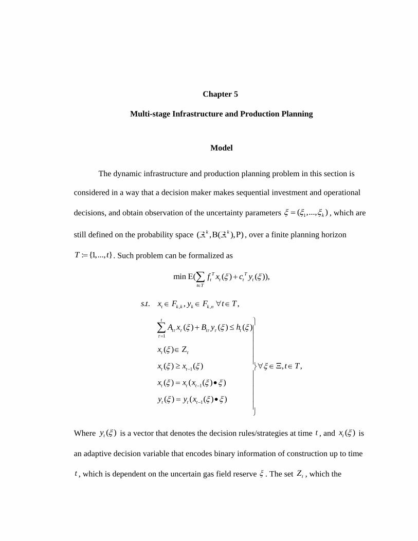
The dynamic infrastructure and production planning problem in this section is

considered in a way that a decision maker makes sequential investment and operational

decisions, and obtain observation of the uncertainty parameters 1( ,..., )k , which are

still defined on the probability space ( , ( ), )k k , over a finite planning horizon

: {1,..., }T t . Such problem can be formalized as

min ( ( ) ( )),T T

t t t t

t T

f x c y

, ,

1

1

1

1

. . , ,

( ) ( ) ( )

( )

( ) ( ) , ,

( ) ( ( ) )

( ) ( ( ) )

t k k k k n

t

t t t

t t

t t

t t t

t t t

s t x F y F t T

A x B y h

x

x x t T

x x x

y y x

Where ( )ty is a vector that denotes the decision rules/strategies at time t , and ( )tx is

an adaptive decision variable that encodes binary information of construction up to time

t , which is dependent on the uncertain gas field reserve . The set tZ , which the

22

adaptive decision variable belongs to is a subset of {0,1}k , as it may include constraints

which enforce the order of the gas field reserve revealed. For example, a platform can

only be built at a certain gas field after another platform is constructed or certain

pipelines can be built only after certain stages. If i is observed and included in the

information base at time t , then , ( ) 1t ix , which will also incur a cost of ,t if and

another term ( )tB y in the time t constraint. The constraint 1( ) ( )t tx x will

enforce that the construction will not be removed, and thus , ( )t ix is monotonous, which

will stay on 1. The last two constraints in the formulation enforce non-anticipativity,

which restrict the decision strategies ( )ty to only depend on gas fields information

obtained up to time 1t .

The above type of problem involves a multi-stage dynamic programming with

adaptive decision rules/strategies and binary recourse variables and is shown to be

computationally intractable. To approximate a conservative solution, linear assumptions

and partition of uncertainty set are therefore necessary.

Approximation

Compared to the one-stage production planning model, the multi-stage is more

complicated and expensive in computing. Past research on multi-stage stochastic

programming has studied the approximation of stochastic programming with continuous

recourse variables, of which conservative solutions could be obtained by linear decision

rules (Ben-Tal et al. 2004). Also, finite adaptability, which is the middle ground of

23

complete adaptability where the decision-maker has arbitrary adaptability to the exact

realization of the uncertainty and static robust formulation where the decision-maker has

no information on the realization of the uncertainty, has also proved tractable and

efficient when solving multi-stage stochastic programming (Bertsimas. D., and

Caramanis, C, 2010). The idea of the approach is partitioning the uncertainty space and

receiving information about the realization of the uncertainty, which provides an

opportunity to trade off computing expense with optimality. Based on this idea, Vayanos

et al. (2011) solve the stochastic programming problem with endogenous uncertainty by

approximating the binary decision rules that are piecewise constant and real-valued

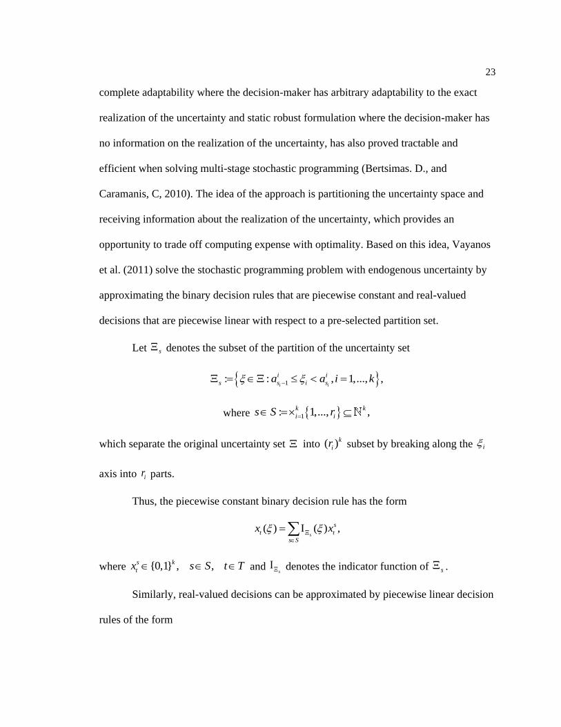
decisions that are piecewise linear with respect to a pre-selected partition set.

Let s denotes the subset of the partition of the uncertainty set

1: : , 1,..., ,i i

i i

s s i sa a i k

where 1: 1,..., ,k k

i is S r

which separate the original uncertainty set into ( )k

ir subset by breaking along the i

axis into ir parts.

Thus, the piecewise constant binary decision rule has the form

( ) ( ) ,s

s

t t

s S

x x

where {0,1} , ,s k

tx s S t T and s

denotes the indicator function of s .

Similarly, real-valued decisions can be approximated by piecewise linear decision

rules of the form

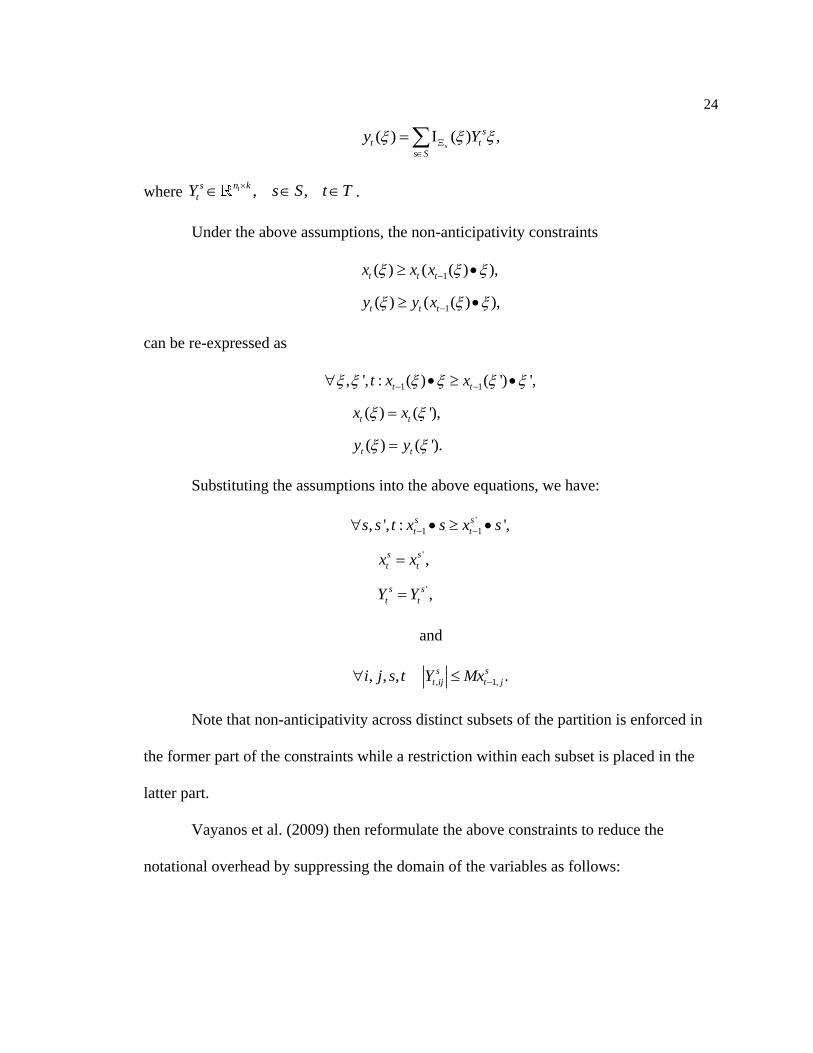
24

( ) ( ) ,s

s

t t

s S

y Y

where , ,tn ks

tY s S t T

.

Under the above assumptions, the non-anticipativity constraints

1

1

( ) ( ( ) ),

( ) ( ( ) ),

t t t

t t t

x x x

y y x

can be re-expressed as

1 1, ', : ( ) ( ') ',

( ) ( '),

( ) ( ').

t t

t t

t t

t x x

x x

y y

Substituting the assumptions into the above equations, we have:

'

1 1

'

'

, ', : ',

,

,

s s

t t

s s

t t

s s

t t

s s t x s x s

x x

Y Y

and

, 1,, , , .s s

t ij t ji j s t Y Mx

Note that non-anticipativity across distinct subsets of the partition is enforced in

the former part of the constraints while a restriction within each subset is placed in the

latter part.

Vayanos et al. (2009) then reformulate the above constraints to reduce the

notational overhead by suppressing the domain of the variables as follows:

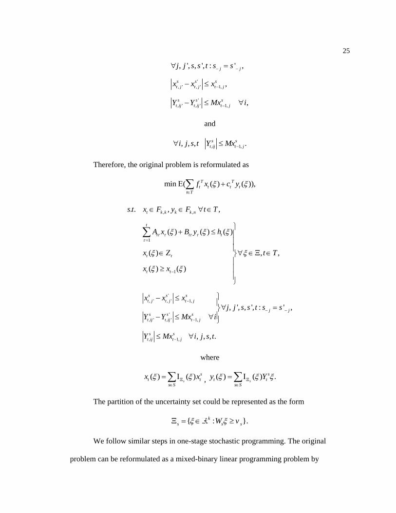
25

'

, ' , ' 1,

'

, ' , ' 1,

, ', , ', : ' ,

,

,

j j

s s s

t j t j t j

s s s

t ij t ij t j

j j s s t s s

x x x

Y Y Mx i

and

, 1,, , , .s s

t ij t ji j s t Y Mx

Therefore, the original problem is reformulated as

min ( ( ) ( )),T T

t t t t

t T

f x c y

, ,

1

1

'

, ' , ' 1,

'

, ' , ' 1,

, 1,

. . , ,

( ) ( ) ( )

( ) , ,

( ) ( )

, ', , ', : ' ,

, , , .

t k k k k n

t

t t t

t t

t t

s s s

t j t j t j

j js s s

t ij t ij t j

s s

t ij t j

s t x F y F t T

A x B y h

x t T

x x

x x x

j j s s t s s

Y Y Mx i

Y Mx i j s t

where

( ) ( )s

s

t t

s S

x x

, ( ) ( ) .s

s

t t

s S

y Y

The partition of the uncertainty set could be represented as the form

{ : }.k

s s sW v

We follow similar steps in one-stage stochastic programming. The original

problem can be reformulated as a mixed-binary linear programming problem by

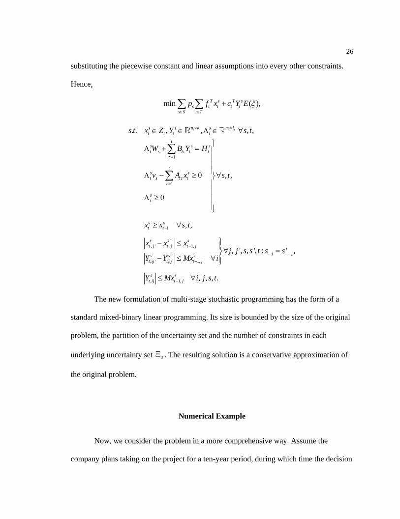
26

substituting the piecewise constant and linear assumptions into every other constraints.

Hence,

min ( ),T s T s

s t t t t

s S t T

p f x c Y E

1

1

1

'

, ' , ' 1,

'

, ' , ' 1,

, 1,

. . , , , ,

0 , ,

0

, ,

, ', , ', : ' ,

t t sn k m ls s s

t t t t

ts s s

t s t t t

ts s

t s t t

s

t

s s

t t

s s s

t j t j t j

j js s s

t ij t ij t j

s

t ij t

s t x Z Y s t

W B Y H

v A x s t

x x s t

x x xj j s s t s s

Y Y Mx i

Y Mx

, , , .s

j i j s t

The new formulation of multi-stage stochastic programming has the form of a

standard mixed-binary linear programming. Its size is bounded by the size of the original

problem, the partition of the uncertainty set and the number of constraints in each

underlying uncertainty set s . The resulting solution is a conservative approximation of

the original problem.

Numerical Example

Now, we consider the problem in a more comprehensive way. Assume the

company plans taking on the project for a ten-year period, during which time the decision

27

maker needs to organize the gas extraction and transportation process. The goal is to

maximize the net present value of the project.

Different from the one-stage problem, the decision maker now has multiple years

to make decisions for gas production. The size of each gas field is not necessarily

revealed in the first period, as the decision maker may choose a later time to reduce the

cost of building the platform. However, the revenue of the sales of gas will also decrease

when the gas is extracted at a later time.

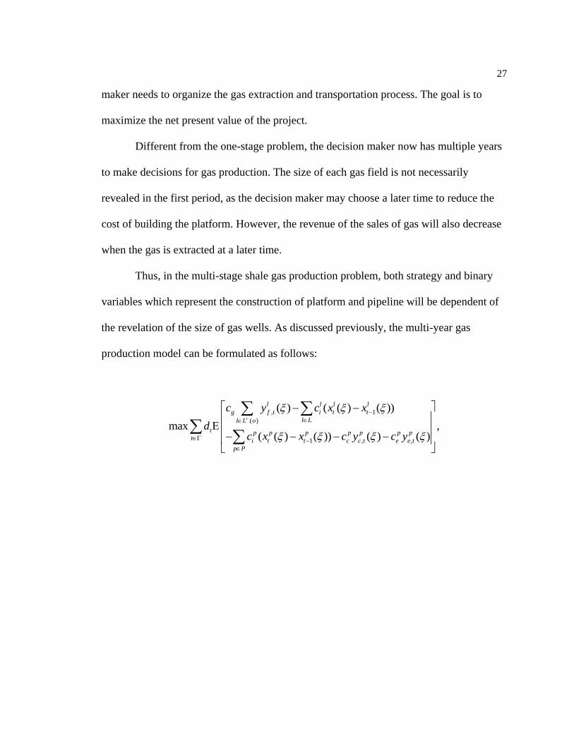
Thus, in the multi-stage shale gas production problem, both strategy and binary

variables which represent the construction of platform and pipeline will be dependent of

the revelation of the size of gas wells. As discussed previously, the multi-year gas

production model can be formulated as follows:

, 1

( )

1 , ,

( ) ( ( ) ( ))

max ,( ( ) ( )) ( ) ( )

l l l l

g f t i t t

l Ll L o

t p p p p p p pt i t t c c t e e t

p P

c y c x x

dc x x c y c y

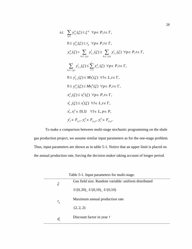
28

,

,

, , ,

( ) ( )

, ,

1( )

,

,

1

. . ( ) , ,

0 ( ) , ,

( ) ( ) ( ) , ,

( ) ( ) , ,

0 ( ) ( ) , ,

0 ( ) ( ) , ,

(

p p

e t

t

p

e t p

p l l

e t f t f t

l L p l L p

tl p

f t c

l L p

l l

f t t

p p

c t t

p

t

s t y p P t

y r p P t

y y y p P t

y y p P t

y Mx l L t

y Mx p P t

x

1

, , ,

) ( ) , ,

( ) ( ) , ,

, {0,1} , ,

, , .

p

t

l l

t t

l p

t t

l p p

f p l e p p c p p

x p P t

x x l L t

x x l L p P

y F y F y F

To make a comparison between multi-stage stochastic programming on the shale

gas production project, we assume similar input parameters as for the one-stage problem.

Thus, input parameters are shown as in table 5-1. Notice that an upper limit is placed on

the annual production rate, forcing the decision maker taking account of longer period.

Table 5-1. Input parameters for multi-stage.

p

Gas field size. Random variable: uniform distributed

(0,20)U , (0,10)U , (0,10)U

pr

Maximum annual production rate

(2, 2, 2)

tdDiscount factor in year t

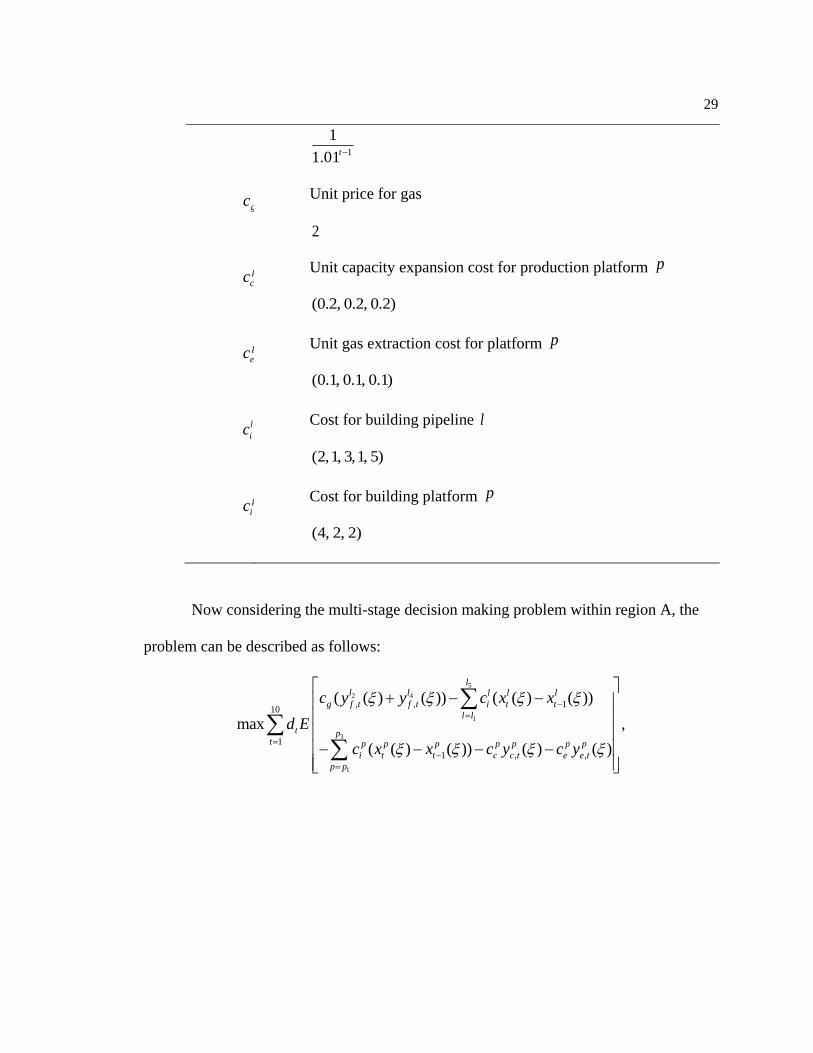
29

1

1

1.01t

gc

Unit price for gas

2

p

cc

Unit capacity expansion cost for production platform p

(0.2, 0.2, 0.2)

p

ec

Unit gas extraction cost for platform p

(0.1, 0.1, 0.1)

l

ic

Cost for building pipeline l

(2,1, 3,1, 5)

p

ic

Cost for building platform p

(4, 2, 2)

Now considering the multi-stage decision making problem within region A, the

problem can be described as follows:

5

2 4

1

3

1

, , 110

1

1 , ,

( ( ) ( )) ( ( ) ( ))

max ,

( ( ) ( )) ( ) ( )

ll l l l l

g f t f t i t t

l l

t pt p p p p p p p

i t t c c t e e t

p p

c y y c x x

d E

c x x c y c y

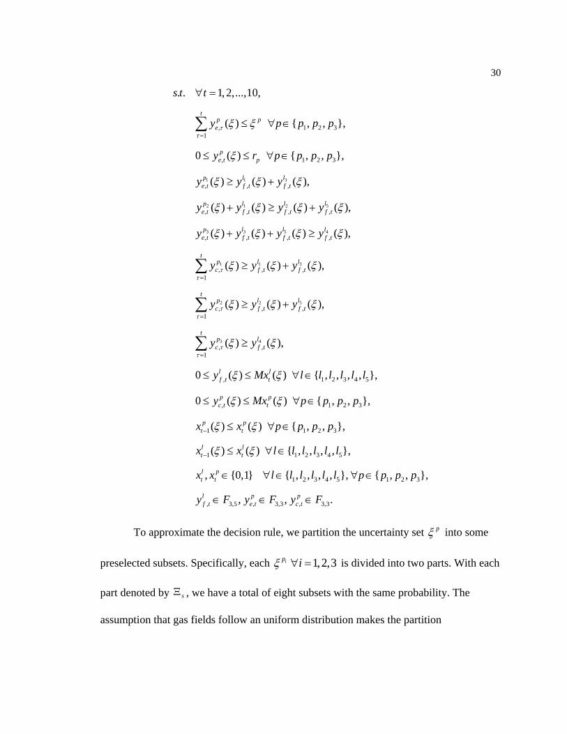
30

31 1

52 1 2

3 3 5 4

1

, 1 2 3

1

, 1 2 3

, , ,

, , , ,

, , , ,

,

1

. . 1, 2,...,10,

( ) { , , },

0 ( ) { , , },

( ) ( ) ( ),

( ) ( ) ( ) ( ),

( ) ( ) ( ) ( ),

( )

tp p

e

p

e t p

lp l

e t f t f t

lp l l

e t f t f t f t

p l l l

e t f t f t f t

tp

c

s t t

y p p p p

y r p p p p

y y y

y y y y

y y y y

y

31

52 2

3 4

, ,

, , ,

1

, ,

1

, 1 2 3 4 5

, 1 2 3

1 1 2 3

1 1

( ) ( ),

( ) ( ) ( ),

( ) ( ),

0 ( ) ( ) { , , , , },

0 ( ) ( ) { , , },

( ) ( ) { , , },

( ) ( ) {

ll

f t f t

tlp l

c f t f t

tp l

c f t

l l

f t t

p p

c t t

p p

t t

l l

t t

y y

y y y

y y

y Mx l l l l l l

y Mx p p p p

x x p p p p

x x l l

2 3 4 5

1 2 3 4 5 1 2 3

, 3,5 , 3,3 , 3,3

, , , , },

, {0,1} { , , , , }, { , , },

, , .

l p

t t

l p p

f t e t c t

l l l l

x x l l l l l l p p p p

y F y F y F

To approximate the decision rule, we partition the uncertainty set p into some

preselected subsets. Specifically, each 1,2,3ipi is divided into two parts. With each

part denoted by s , we have a total of eight subsets with the same probability. The

assumption that gas fields follow an uniform distribution makes the partition

31

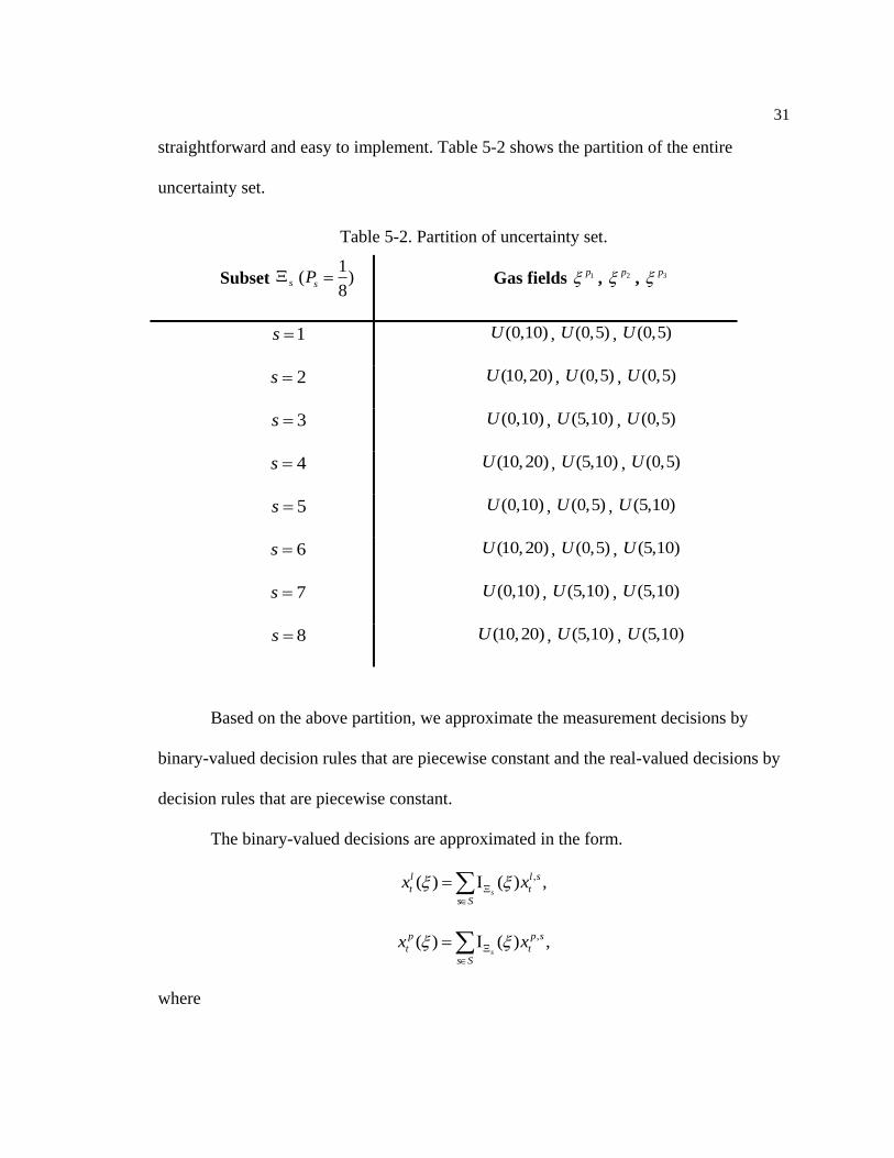
straightforward and easy to implement. Table 5-2 shows the partition of the entire

uncertainty set.

Table 5-2. Partition of uncertainty set.

Subset s1

( )8

sP Gas fields 1p , 2p , 3p

1s (0,10)U , (0,5)U , (0,5)U

2s (10,20)U , (0,5)U , (0,5)U

3s (0,10)U , (5,10)U , (0,5)U

4s (10,20)U , (5,10)U , (0,5)U

5s (0,10)U , (0,5)U , (5,10)U

6s (10,20)U , (0,5)U , (5,10)U

7s (0,10)U , (5,10)U , (5,10)U

8s (10,20)U , (5,10)U , (5,10)U

Based on the above partition, we approximate the measurement decisions by

binary-valued decision rules that are piecewise constant and the real-valued decisions by

decision rules that are piecewise constant.

The binary-valued decisions are approximated in the form.

,( ) ( ) ,s

l l s

t t

s S

x x

,( ) ( ) ,s

p p s

t t

s S

x x

where

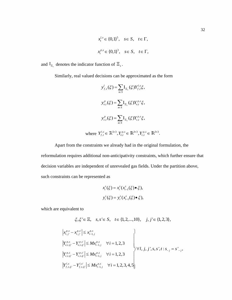
32

, 5{0,1} , , ,l s

tx s S t

, 3{0,1} , , ,p s

tx s S t

and s

denotes the indicator function of s .

Similarly, real valued decisions can be approximated as the form

,

, ,( ) ( ) ,s

l l s

f t f t

s S

y Y

,

, ,( ) ( ) ,s

p p s

e t e t

s S

y Y

,

, ,( ) ( ) ,s

p p s

c t c t

s S

y Y

where , 5 3 , 3 3 , 3 3

, , ,, , .l s p s p s

f t e t c tY Y Y

Apart from the constraints we already had in the original formulation, the

reformulation requires additional non-anticipativity constraints, which further ensure that

decision variables are independent of unrevealed gas fields. Under the partition above,

such constraints can be represented as

1

1

( ) ( ( ) ),

( ) ( ( ) ),

s s s

t t t

s s s

t t t

x x x

y y x

which are equivalent to

, ' , , ' , {1,2,...,10}, , ' {1,2,3},s s S t j j

, , ' ,

, ' , ' 1,

, , ' ,

, , ' , , ' 1,

, , ' ,

, , ' , , ' 1,

, , ' ,

, , ' , , ' 1,

1,2,3

, , ', , ', : ' ,

1,2,3

1,2,3,4,5

p s p s p s

t j t j t j

p s p s p s

e t ij e t ij t j

j jp s p s p s

c t ij c t ij t j

l s l s p s

f t ij f t ij t j

x x x

Y Y Mx i

l j j s s t s s

Y Y Mx i

Y Y Mx i

33

, ,

, , 1,

, ,

, , 1,

, ,

, , 1,

, , , ,

l s p s

f t ij t j

p s p s

e t ij t j

p s p s

c t ij t j

Y Mx

Y Mx i j s t

Y Mx

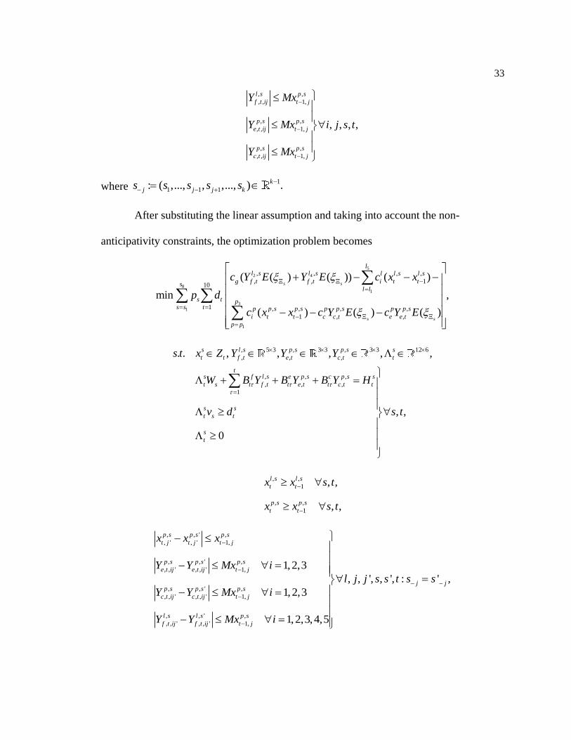
where 1

1 1 1: ( ,..., , ,..., ) .k

j j j ks s s s s

After substituting the linear assumption and taking into account the non-

anticipativity constraints, the optimization problem becomes

5

2 4

81

3

1

1

, , , ,

, , 110

1 , , , ,

1 , ,

( ( ) ( )) ( )

min ,

( ) ( ) ( )

s s

s s

ll s l s l l s l s

g f t f t i t tsl l

s t ps s t p p s p s p p s p p s

i t t c c t e e t

p p

c Y E Y E c x x

p d

c x x c Y E c Y E

, 5 3 , 3 3 , 3 3 12 6

, , ,

, , ,

, , ,

1

. . , , , , ,

, ,

0

s l s p s p s s

t t f t e t c t t

ts f l s e p s c p s s

t s t f t t e t t c t t

s s

t s t

s

t

s t x Z Y Y Y

W B Y B Y B Y H

v d s t

, ,

1

, ,

1

, ,

, ,

l s l s

t t

p s p s

t t

x x s t

x x s t

, , ' ,

, ' , ' 1,

, , ' ,

, , ' , , ' 1,

, , ' ,

, , ' , , ' 1,

, , ' ,

, , ' , , ' 1,

1,2,3

, , ', , ', : ' ,

1,2,3

1,2,3,4,5

p s p s p s

t j t j t j

p s p s p s

e t ij e t ij t j

j jp s p s p s

c t ij c t ij t j

l s l s p s

f t ij f t ij t j

x x x

Y Y Mx i

l j j s s t s s

Y Y Mx i

Y Y Mx i

34

, ,

, , 1,

, ,

, , 1,

, ,

, , 1,

, , , ,

l s p s

f t ij t j

p s p s

e t ij t j

p s p s

c t ij t j

Y Mx

Y Mx i j s t

Y Mx

, ' , , ' , {1,2,...,10}, , ' {1,2,3}.s s S t j j

The above optimization problem is a standard mixed-integer programming with

its size bounded by the size of the original problem, the partition of the uncertainty set

and the number of constraints in each underlying uncertainty set s . I use GAMS with

CPLEX solver to solve the problem. It takes the software 5 seconds to obtain the result.

Some optimal results of decision variables are indicated and explained below.

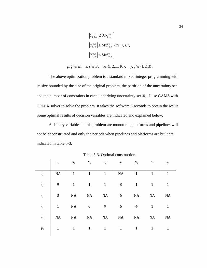
As binary variables in this problem are monotonic, platforms and pipelines will

not be deconstructed and only the periods when pipelines and platforms are built are

indicated in table 5-3.

Table 5-3. Optimal construction.

1s 2s 3s 4s 5s 6s 7s 8s

1l NA 1 1 1 NA 1 1 1

2l 9 1 1 1 8 1 1 1

3l 3 NA NA NA 6 NA NA NA

4l 1 NA 6 9 6 4 1 1

5l NA NA NA NA NA NA NA NA

1p 1 1 1 1 1 1 1 1

35

2p 1 1 1 1 1 1 1 1

3p 1 3 1 1 2 3 1 1

The numbers in the table indicate the index of period t .

NA means the pipeline/platform is not built under this scenario.

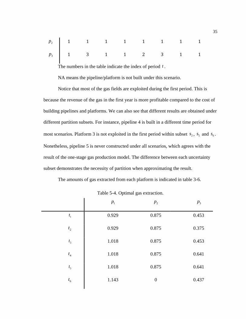
Notice that most of the gas fields are exploited during the first period. This is

because the revenue of the gas in the first year is more profitable compared to the cost of

building pipelines and platforms. We can also see that different results are obtained under

different partition subsets. For instance, pipeline 4 is built in a different time period for

most scenarios. Platform 3 is not exploited in the first period within subset 2s , 5s and 6s .

Nonetheless, pipeline 5 is never constructed under all scenarios, which agrees with the

result of the one-stage gas production model. The difference between each uncertainty

subset demonstrates the necessity of partition when approximating the result.

The amounts of gas extracted from each platform is indicated in table 3-6.

Table 5-4. Optimal gas extraction.

1p 2p 3p

1t 0.929 0.875 0.453

2t 0.929 0.875 0.375

3t 1.018 0.875 0.453

4t 1.018 0.875 0.641

5t 1.018 0.875 0.641

6t 1.143 0 0.437

36

7t 1.143 0 0.438

8t 0.964 0.104 0.437

9t 0.964 0.229 0.375

10t 0.875 0.229 0.375

Total 10.001 4.937 4.625

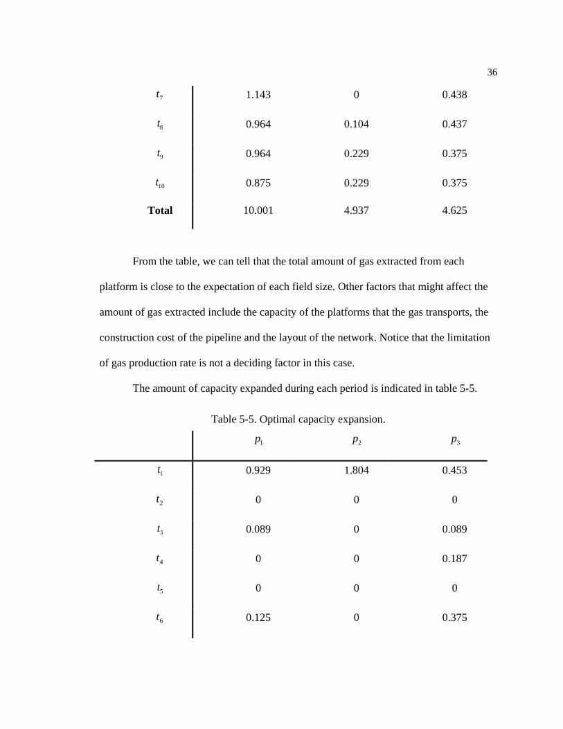
From the table, we can tell that the total amount of gas extracted from each

platform is close to the expectation of each field size. Other factors that might affect the

amount of gas extracted include the capacity of the platforms that the gas transports, the

construction cost of the pipeline and the layout of the network. Notice that the limitation

of gas production rate is not a deciding factor in this case.

The amount of capacity expanded during each period is indicated in table 5-5.

Table 5-5. Optimal capacity expansion.

1p 2p 3p

1t 0.929 1.804 0.453

2t 0 0 0

3t 0.089 0 0.089

4t 0 0 0.187

5t 0 0 0

6t 0.125 0 0.375

37

7t 0 0 0

8t 0 0.104 0

9t 0 0.125 0.125

10t 0 0 0

Total 1.143 2.033 1.229

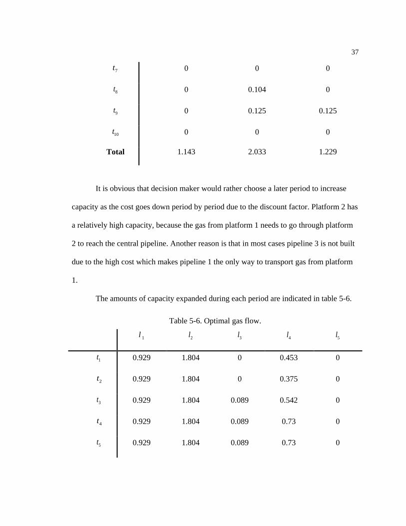
It is obvious that decision maker would rather choose a later period to increase

capacity as the cost goes down period by period due to the discount factor. Platform 2 has

a relatively high capacity, because the gas from platform 1 needs to go through platform

2 to reach the central pipeline. Another reason is that in most cases pipeline 3 is not built

due to the high cost which makes pipeline 1 the only way to transport gas from platform

1.

The amounts of capacity expanded during each period are indicated in table 5-6.

Table 5-6. Optimal gas flow.

1l 2l 3l 4l 5l

1t 0.929 1.804 0 0.453 0

2t 0.929 1.804 0 0.375 0

3t 0.929 1.804 0.089 0.542 0

4t 0.929 1.804 0.089 0.73 0

5t 0.929 1.804 0.089 0.73 0

38

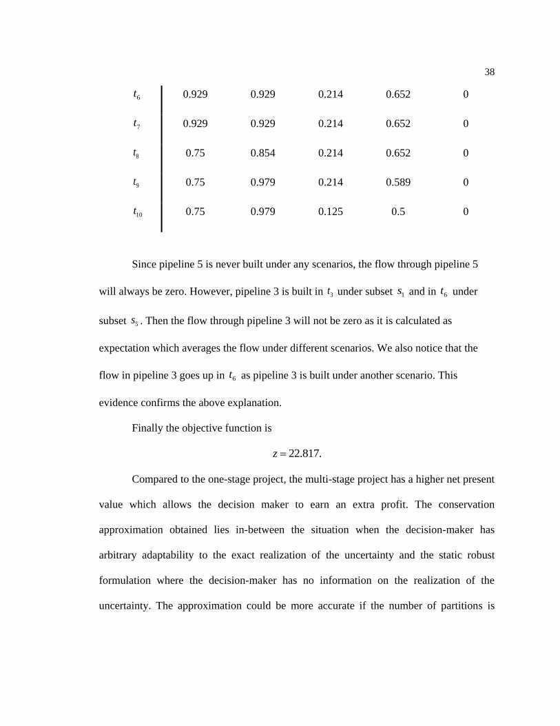
6t 0.929 0.929 0.214 0.652 0

7t 0.929 0.929 0.214 0.652 0

8t 0.75 0.854 0.214 0.652 0

9t 0.75 0.979 0.214 0.589 0

10t 0.75 0.979 0.125 0.5 0

Since pipeline 5 is never built under any scenarios, the flow through pipeline 5

will always be zero. However, pipeline 3 is built in 3t under subset 1s and in 6t under

subset 5s . Then the flow through pipeline 3 will not be zero as it is calculated as

expectation which averages the flow under different scenarios. We also notice that the

flow in pipeline 3 goes up in 6t as pipeline 3 is built under another scenario. This

evidence confirms the above explanation.

Finally the objective function is

22.817.z

Compared to the one-stage project, the multi-stage project has a higher net present

value which allows the decision maker to earn an extra profit. The conservation

approximation obtained lies in-between the situation when the decision-maker has

arbitrary adaptability to the exact realization of the uncertainty and the static robust

formulation where the decision-maker has no information on the realization of the

uncertainty. The approximation could be more accurate if the number of partitions is

39

increased. However, this will also increase the computing cost as the size of the problem

is dependent on the partition.

Chapter 6

Conclusions and Future Work

The shale gas infrastructure and production planning problem is discussed in this

paper. The problem is modeled as stochastic programming with endogenous

uncertainties. Approximations using the adaptive measurement decisions by piecewise

constant functions and the adaptive real-valued decisions by piecewise linear functions of

the uncertainties could be applied to obtain conservative solutions.

The decision rule approximation successfully solves the problem with

continuously distributed uncertainty parameters. The approximation is considered close

to optimal and can be improved by increasing the partition of the uncertainty set. A one-

stage numerical is equivalent to a static problem where each field size equals the

expectation of the underlying uncertainty parameter. Results of the multi-stage numerical

experiment are reasonable. Decision makers are able to obtain more profit by taking on

the project for multiple years.

Future work can improve the sophistication of the shale gas infrastructure. A

more complicated network with a longer investigating time horizon can be considered to

better fit the context of shale gas production. The partition of subset maybe increased if

necessary to obtain more accurate solution.

List of References

Barnes, R. J., Linke, P., & Kokossis, A., Optimization of oil-field development

production capacity. European Symposium on Computer Aided Process Engineering, 12,

631 (2002).

Ben-Tal, A., Boyd, S., and Nemirovski, A. Extending scope of robust

optimization: com-prehensive robust counterparts of uncertain problems. Math. Program.

107, 1-2, Ser. B (2006), 63–89.

Ben-Tal, A., Goryashko, A., Guslitzer, E., and Nemirovski, A. Adjustable robust

solutions of uncertain linear programs. Math. Program. 99, 2, Ser. A (2004), 351–376.

Bertsimas. D., and Caramanis, C. Finite adaptability for linear optimization, IEEE

Trans. Automat. Contr., vol. 55, no. 12, pp. 2751–2766, 2010.

Considine, T., and Watson, R. An Emerging Giant: Prospects and Economic

Impacts of Developing the Marcellus Shale Natural Gas Play (2009).

Considine, T., and Watson, R., Blumsack, S. The Economic Impacts of the

Pennsylvania Marcellus Shale Natural Gas Play: An Update (2010).

Dyer, M., and Stougie, L. Computational complexity of stochastic programming

problems. Math. Program. A 106, 3 (2006), 423–432.

Goh, J., and Sim, M., Distributionally robust optimization and its tractable

approximations, Oper. Res. vol. 58, no. 4, pp. 902–917, 2010.

42

Haugen, K. K., A stochastic dynamic programming model for scheduling of

offshore petroleum fields with resource uncertainty. European Journal of Operational

Research, 88, 88 (1996).

Ierapetritou, M. G., Floudas, C. A., Vasantharajan, S., & Cullick, A. S. Optimal

location of vertical wells: A decomposition approach. AIChE Journal, 45, 844 (1998).

Iyer, R. R., Grossmann, I. E., Vasantharajan, S., & Cullick, A. S. Optimal

planning and scheduling of offshore oil field infrastructure investment and operations.

Industrial and Engineering Chemistry Research, 37, 1380 (1998).

Jonsbraten, T., Optimization models for petroleum field exploitation, Ph.D.

dissertation, Norwegian Shool of Economics and Business Administration (1998).

Kosmidis, V. D., Perkins, J. D., & Pistikopoulos, E. N. A mixed integer

optimization strategy for integrated gas/oil production. European Symposium on

Computer Aided Process Engineering, 12, 697 (2002).

Kuhn, D., Wiesemann, W., and Georghiou, A., Primal and dual linear decision

rules in stochastic and robust optimization, Mathematical Programming, 2009.

Lin, X., & Floudas, C. A., A novel continuous-time modeling and optimization

framework for well platform planning problems. Optimization and Engineering, 4, 65–93

(2003).

Meister, B., Clark, J. M. C., & Shah, N., Optimization of oil-field exploitation

under uncertainty. Computers and Chemical Engineering, 20(ser. B), S1251 (1996).

43

Ortiz-Gomez, A., Rico-Ramirez, V., & Hernandez-Castro, S., Mixed-integer

multi-period model for the planning of oil-field production. Computers and Chemical

Engineering, 26(4–5), 703 (2002).

Shapiro, A., and Nemirovski, A. On complexity of stochastic programming

problems. In Continuous Optimization: Current Trends and Applications (2005), V.

Jeyakumar and A. Rubinov, Eds., Springer, pp. 111–144.

Vayanos. P., Kuhn, D., and Rustem, B. Decision rules for information discovery

in multi-stage stochastic programming. IEEE CDC-ECC (2011).