Multi-slice helical CT: Scan and reconstructionHui Hua),b)

General Electric Company, Applied Science Laboratory, Milwaukee, Wisconsin 53201-0414

~Received 21 April 1998; accepted for publication 27 October 1998!

The multi-slice CT scanner refers to a special CT system equipped with a multiple-row detectorarray to simultaneously collect data at different slice locations. The multi-slice CT scanner has thecapability of rapidly scanning large longitudinal~z! volume with highz-axis resolution. It alsopresents new challenges and new characteristics. In this paper, we study the scan and reconstructionprinciples of the multi-slice helical CT in general and the 4-slice helical CT in particular. Themulti-slice helical computed tomography consists of the following three key components: the pre-ferred helical pitches for efficientz sampling in data collection and better artifact control; the newhelical interpolation algorithms to correct for fast simultaneous patient translation; and thez-filtering reconstruction for providing multiple tradeoffs of the slice thickness, image noise andartifacts to suit for different application requirements. The concept of the preferred helical pitch isdiscussed with a newly proposedz sampling analysis. New helical reconstruction algorithms andz-filtering reconstruction are developed for multi-slice CT in general. Furthermore, the theoreticalmodels of slice profile and image noise are established for multi-slice helical CT. For 4-slice helicalCT in particular, preferred helical pitches are discussed. Special reconstruction algorithms aredeveloped. Slice profiles, image noises, and artifacts of 4-slice helical CT are studied and comparedwith single slice helical CT. The results show that the slice profile, image artifacts, and noiseexhibit performance peaks or valleys at certain helical pitches in the multi-slice CT, whereas in thesingle-slice CT the image noise remains unchanged and the slice profile and image artifacts steadilydeteriorate with helical pitch. The study indicates that the 4-slice helical CT can provide equivalentimage quality at 2 to 3 times the volume coverage speed of the single slice helical CT. ©1999American Association of Physicists in Medicine.@S0094-2405~99!00401-0#

Key words: multi-slice CT, helical/spiral CT, preferred helical pitch, multi-slice helicalinterpolation algorithms,z-filtering reconstruction, the volume coverage speed performance,theoretical models

is aca-

edce-

n;ain

ed

pa-eedan-ed.ing,%

I. INTRODUCTION

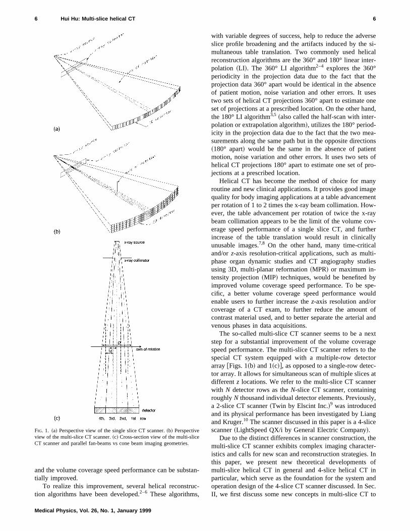
Most currently used x-ray CT scanners are the single slfan-beam CT system. In this system, the x-ray photons emnating from the focal spot of the x-ray tube are first collmated into a thin fan shaped beam@Fig. 1~a!#. After attenu-ation by the object being imaged, the attenuation profilethis fan-beam, also called the fan-beam projection, iscorded by a single row of detector array, consistingroughly a thousand detector elements.

There are two modes for a CT scan: step-and-shoot CThelical ~or spiral! CT. For step-and-shoot CT, it consists otwo alternate stages: data acquisition and patient positionDuring the data acquisition stage, the patient remains statiary and the x-ray tube rotates about the patient to acquircomplete set of projections at a prescribed scanning locatDuring the patient positioning stage, no data are acquiand the patient is transported to the next prescribed scannlocation. The data acquisition stage typically takes one sond or less while the patient positioning stage is around osecond. Thus, the duty cycle of the step-and-shoot CT50% at best. This poor scanning efficiency directly limits thvolume coverage speed versus performance and thereforescan throughput of the step-and-shoot CT.

The term volume coverage speed versus performance~or

5 Med. Phys. 26 „1…, January 1999 0094-2405/99/26

icea-

i-

ofre-of

orf

ing.on-e aion.reding

ec-neisethe

the volume coverage speed performance for short! refers tothe capability of rapidly scanning a large longitudinal~z!volume with high longitudinal~z-axis! resolution and lowimage artifacts. The volume coverage speed performancedeciding factor for the success of many medical CT applitions which require a large volume scanning~e.g., an entireliver or lung! with high image quality~i.e., highz-axis reso-lution and low image artifacts! and short time duration. Thetime duration is usually a fraction of a minute and is imposby ~1! short scan duration for improved contrast enhanment and for reduced usage of the contrast material;~2! pa-tient breathhold period for reduced respiratory motioand/or ~3! maximum scan duration without experiencinglengthy tube cooling delay. Thus, one of the main themesCT development is to improve its volume coverage speperformance.

Helical ~or spiral! CT1–4 was introduced around 1990. Inthis mode, the data are continuously acquired while thetient is simultaneously transported at a constant spthrough the gantry. The patient translating distance per gtry rotation in helical scan is referred to as the table speBecause the data are continuously collected without pausthe duty cycle of the helical scan is improved to nearly 100

5„1…/5/14/$15.00 © 1999 Am. Assoc. Phys. Med.

t

c

rsei-alr-

eces

ned,

-ns

ntofo-

yent-ay-er

y

-ies

pe-ld

ofand

xtgeher

-t

r

y,

ngce

er-Inof

ndec.o

6 Hui Hu: Multi-slice helical CT 6

and the volume coverage speed performance can be substially improved.

To realize this improvement, several helical reconstrution algorithms have been developed.2–6 These algorithms,

FIG. 1. ~a! Perspective view of the single slice CT scanner.~b! Perspectiveview of the multi-slice CT scanner.~c! Cross-section view of the multi-sliceCT scanner and parallel fan-beams vs cone beam imaging geometries.

Medical Physics, Vol. 26, No. 1, January 1999

an-

-

with variable degrees of success, help to reduce the adveslice profile broadening and the artifacts induced by the smultaneous table translation. Two commonly used helicreconstruction algorithms are the 360° and 180° linear intepolation ~LI !. The 360° LI algorithm2–4 explores the 360°periodicity in the projection data due to the fact that thprojection data 360° apart would be identical in the absenof patient motion, noise variation and other errors. It usetwo sets of helical CT projections 360° apart to estimate oset of projections at a prescribed location. On the other hanthe 180° LI algorithm3,5 ~also called the half-scan with inter-polation or extrapolation algorithm!, utilizes the 180° period-icity in the projection data due to the fact that the two measurements along the same path but in the opposite directio~180° apart! would be the same in the absence of patiemotion, noise variation and other errors. It uses two setshelical CT projections 180° apart to estimate one set of prjections at a prescribed location.

Helical CT has become the method of choice for manroutine and new clinical applications. It provides good imagquality for body imaging applications at a table advancemeper rotation of 1 to 2 times the x-ray beam collimation. However, the table advancement per rotation of twice the x-rbeam collimation appears to be the limit of the volume coverage speed performance of a single slice CT, and furthincrease of the table translation would result in clinicallunusable images.7,8 On the other hand, many time-criticaland/orz-axis resolution-critical applications, such as multiphase organ dynamic studies and CT angiography studusing 3D, multi-planar reformation~MPR! or maximum in-tensity projection~MIP! techniques, would be benefited byimproved volume coverage speed performance. To be scific, a better volume coverage speed performance wouenable users to further increase thez-axis resolution and/orcoverage of a CT exam, to further reduce the amountcontrast material used, and to better separate the arterialvenous phases in data acquisitions.

The so-called multi-slice CT scanner seems to be a nestep for a substantial improvement of the volume coveraspeed performance. The multi-slice CT scanner refers to tspecial CT system equipped with a multiple-row detectoarray@Figs. 1~b! and 1~c!#, as opposed to a single-row detector array. It allows for simultaneous scan of multiple slices adifferent z locations. We refer to the multi-slice CT scannewith N detector rows as theN-slice CT scanner, containingroughlyN thousand individual detector elements. Previousla 2-slice CT scanner~Twin by Elscint Inc.!9 was introducedand its physical performance has been investigated by Liaand Kruger.10 The scanner discussed in this paper is a 4-sliscanner~LightSpeed QX/i by General Electric Company!.

Due to the distinct differences in scanner construction, thmulti-slice CT scanner exhibits complex imaging characteistics and calls for new scan and reconstruction strategies.this paper, we present new theoretical developmentsmulti-slice helical CT in general and 4-slice helical CT inparticular, which serve as the foundation for the system aoperation design of the 4-slice CT scanner discussed. In SII, we first discuss some new concepts in multi-slice CT t

f-

lee

y

-e-.

-mp-

of

m-

-

tsd

-

d

s--dt

e

nd

7 Hui Hu: Multi-slice helical CT 7

set the stage for discussion. In Sec. III, we investigateimportant characteristic in multi-slice helical CT daacquisition—preferred helical pitch. In Sec. IV, we presethe helical reconstruction algorithms for the multi-slice CIn Sec. V, we establish the theoretical models of noise aslice profile of the multi-slice CT and assess the performaof the 4-slice CT scanner using these models and compsimulations.

II. NEW CONCEPTS IN MULTI-SLICE CT

Compared with its single slice counterpart, the multi-sliCT is intrinsically more complex and introduces several nconcepts. We discuss two new concepts in this section.

A. Detector row collimation versus x-ray collimation

In the single slice CT@see Fig. 1~a!#, the x-ray beamcollimation ~or, the thickness of the x-ray beam! affects boththe z volume coverage speed and thez-axis resolution~theslice thickness!. A thick x-ray collimation is preferred forlarge volume coverage speed while a thin collimation is dsirable for highz-axis resolution. The single slice CT useare confronted with the conflicting requirements when bolarge volume coverage speed and highz-axis resolution areneeded. In the single slice CT, the detector row collimatis either not used or used as a part of the x-ray beam cmation ~i.e., the post-patient collimation!.

One of the enabling components in multi-slice CT systeis the multi-row detector array. The use of multiple detecrows enables us to further divide the total x-ray beam~stillprescribed by the x-ray beam collimation! into multiple sub-divided beams~prescribed by the detector row collimatioalso called the detector row aperture!, referring to Figs. 1~b!and 1~c!. In the multi-slice CT system, while the total x-racollimation still indicates the volume coverage speed,detector row collimation, rather than the total x-ray collimtion, determines thez-axis resolution~i.e., the slice thick-ness!.

With reference to Figs. 1~b! and 1~c!, we useD andd todenote the x-ray beam collimation and the detector row climation, respectively. Consistent with the convention, boD andd are measured at the axis of rotation. If the gaps~i.e.,the dead area! between adjacent detector rows are small acan be ignored, the detector row spacing equals to the detor row collimation, also denoted asd. The detector rowcollimation ~or spacing!, d, and the x-ray beam collimationD, has the following relationship:

d~mm!5D~mm!

N, ~1!

whereN is the number of detector rows.In single slice CT, the detector row collimation equals

the x-ray beam collimation and these two parameters canused interchangeably. In the multi-slice CT, the detector rcollimation is only 1/N of the x-ray beam collimation. Thismuch improved~relaxed! relationship makes it possible tsimultaneously achieve high volume coverage speed

Medical Physics, Vol. 26, No. 1, January 1999

antantT.nd

nceuter

ceew

e-rsth

ionolli-

mtor

n

ythea-

ol-th

ndtec-

,

tobe

ow

oand

high z-axis resolution. In general, the larger the number odetector rowsN, the better the volume coverage speed performance.

B. Cone-beam geometry versus parallel fan-beamsgeometry

The x-ray photons emanating from the focal spot of thex-ray tube describe a divergent beam. We use the ray bundto capture the effect of the area integration due to the finitsize ~i.e., aperture! of detector cells. The effective trace ofeach ray bundle is described by the center line of the rabundle, as shown in Figs. 1~a!, 1~b!, and 1~c! by the lightdashed lines.

In the single slice CT, the ray bundles lie in the gantryplane—the plane normal to the axis of gantry rotation. However, they fan out within the gantry plane and this divergencis correctly accounted for by the fan-beam imaging geometry, which calls for the fan-beam reconstruction algorithm

In the multi-slice CT@referring to Figs. 1~b! and 1~c!#, theray bundles not only fan out within the gantry plane but alsodiverge from the gantry plane. This imaging geometry iscalled the cone-beam imaging geometry, which calls for special cone-beam reconstruction algorithms. Many cone-beareconstruction algorithms have been developed for both steand-shoot CT11,12 and helical CT.13–15 All of them requirefundamentally different data processing schemes from thatthe existing fan-beam reconstruction.

Because the scanner discussed has a relatively small nuber of detector rows (N54) and therefore relatively smallcone-beam divergent effect, we use the multiple, parallel fanbeams, as illustrated in Fig. 1~c!, to approximate the cone-beam geometry. To be specific, the projection measuremenby each detector row are treated as if they were acquirewith a fan-beam within the gantry plane at the axial locationwhere the subdivided x-ray beam intercepts the axis of rotation, referring to the dark dashed line in Fig. 1~c!. This ap-proximation allows the use of the existing fan-beam basecomputing system.

III. MULTI-SLICE HELICAL CT DATA ACQUISITION:PREFERRED HELICAL PITCHES

Data acquisition and image reconstruction are the two apects of CT that affect the quality of the reconstructed images. The multi-slice helical CT data acquisition is discussein this section and the image reconstruction is in the nexsection.

A. Extended definition of the helical pitch

The pitch of a helical scan refers to the ratio of the tabletranslating distance per gantry rotation to the thickness of thindividual x-ray beam. Letp and s be the helical pitch andtable translating distance per gantry rotation, respectively. Ithe single slice CT, the x-ray beam thickness is determineby the beam collimation setting. The helical pitch for singleslice CT is defined as

,

n.-of

on

in

r-

8 Hui Hu: Multi-slice helical CT 8

p5s~mm!

D~mm!. ~2a!

On the other hand, in the multi-slice CT, the thickness of tindividual x-ray beam is determined by the detector row colimation, as opposed to the x-ray beam collimation. Thus, tdefinition of the helical pitch for the multi-slice CT can beextended as

p5s~mm!

d~mm!. ~2b!

For example, a 4-slice CT scan using 5 mm row collimatio~and therefore 20 mm x-ray beam collimation! and at 15 mmtable translating distance per rotation will result in a helicpitch of 3(515/5) rather than 0.75(515/20).

It is noted that with reference to Eq.~1!, the definition ofthe helical pitch for the multi-slice CT@Eq. 2~b!# reduces tothat for the single slice CT@Eq. 2~a!# when the single sliceCT is considered. It is also noted that consistent with tsingle slice CT definition, the helical pitch of the multi-sliceCT still indicates roughly the number of contiguous slicethat can be generated over the table translating distanceone gantry rotation.

B. Preferred helical pitch

One characteristic in the multi-slice helical CT data aquisition is the existence of the preferred helical pitch. Duto the use of multi-row detector array, projection data alona given path may be measured multiple times by differedetector rows. One important consideration in multi-slice hlical CT data acquisition is to select a preferred helical pitcto reduce the redundant measurements and therefore toprove the overall dataz sampling efficiency. In this section,we first review the single slice helical CT and propose a nez sampling analysis method. We then investigate the concof preferred helical pitch in the multi-slice helical CT datacquisition using thez sampling analysis.

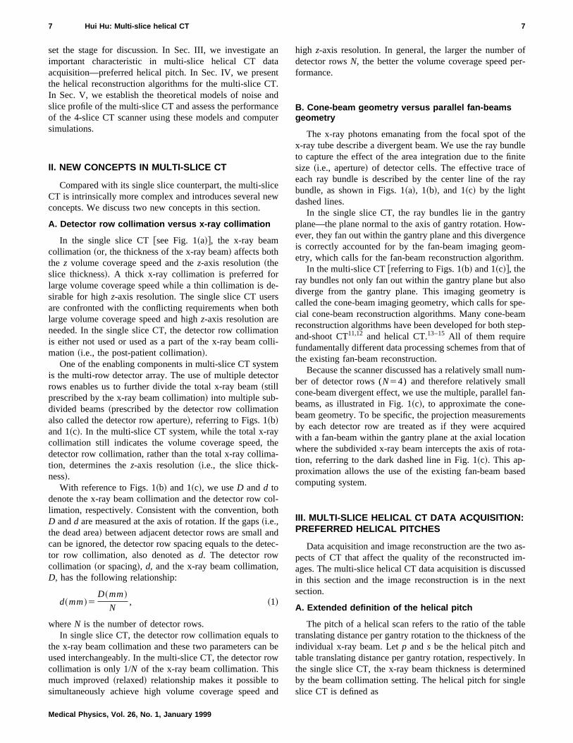
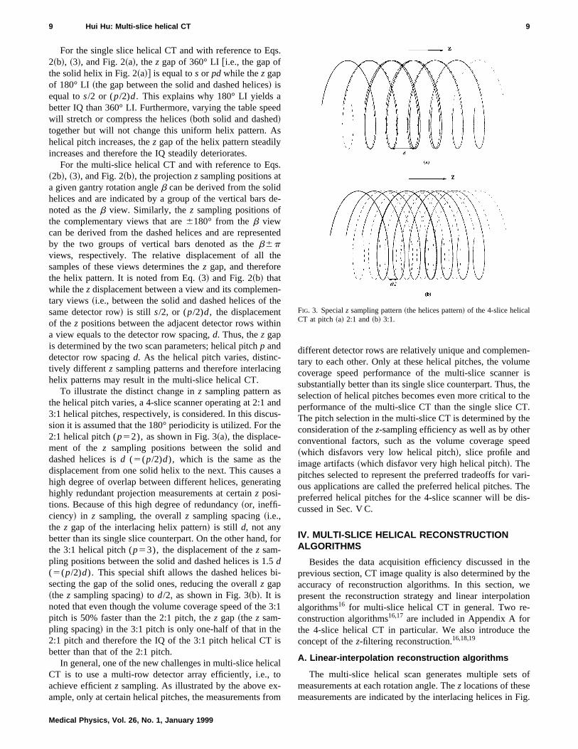
In the single slice helical scan, the x-ray beam describespiral path~i.e., a helix! around the patient, as shown by thsolid line in Fig. 2~a!. Each point on the helix represents a sof fan-beam projection measurements, where the gantrytation angle and thez location of the fan-beam are denoteby the rotation angle and thez position of the helix. Further-more, as mentioned in the Introduction, the projection daexhibit the 180° periodicity that the two measurements alothe same path in the opposite directions would be identicathe absence of patient motion, noise variation, and otherrors. By exploring this 180° periodicity, actual fan-beammeasurements can be regrouped to generate a set of commentary fan-beam projections, which is illustrated by thdashed helix in Fig. 2~a!.

Similarly, in the multi-slice helical CT, the multiple sub-divided x-ray beams defined by multiple~N! detector rowsdescribe multiple~N! interlacing helices. The helices representing different detector rows are shown by the differenshaded solid lines in Fig. 2~b!. Furthermore, utilizing the180° periodicity results in additional complementary fan

Medical Physics, Vol. 26, No. 1, January 1999

hel-he

n

al

he

sin

c-egnte-him-

wepta

s aeetro-d

tangl iner-

ple-e

-tly

-

beam projections, which are illustrated by the multipledifferently-shaded, dashed helices in Fig. 2~b!. These inter-lacing helices form one set of multi-slice helical CT data.

The z gap of the helix pattern represents thez samplingspacing of the projection data to be used in the interpolatioThus, thez gap of the helix pattern determines the effectiveness of the interpolation and therefore is a good indicatorthe image quality~IQ! ~in terms of the slice profile and im-age artifacts!. The smaller thez gap, the better the IQ of thehelical CT. We propose to use thez gap to characterize theIQ of helical CT and call this method thez sampling analy-sis.

Thez gap information can be derived from thez samplingpositions. We useb0 to denote the gantry rotation anglewhen the table is at locationz0 . Thus, thez sampling posi-tions of the measurements acquired at the gantry rotatiangleb is given by the following equation:

z5z01s

2p~b2b0!2Znd, ~3a!

where

Zn5S 2N11

21nD . ~3b!

In Eq. 3~a!, the second term describes the table translationhelical CT as the gantry rotates. The third term depicts thezdisplacements from the gantry plane due to the use of diffeent detector rows. For example,Zn50 for the single sliceCT; Zn5@21.5,20.5,0.5,1.5# for the 4-slice CT@referringto Fig. 1~c!#. n is the detector row index, ranging from 1 toN.

FIG. 2. Illustration of thez sampling pattern~the helices pattern! resultingfrom the ~a! single slice helical CT and~b! multi-slice helical CT.

d

uh

s

-eisee.

ed

ri-e-

ee

n

f

g.

9 Hui Hu: Multi-slice helical CT 9

For the single slice helical CT and with reference to Eq2~b!, ~3!, and Fig. 2~a!, thez gap of 360° LI@i.e., the gap ofthe solid helix in Fig. 2~a!# is equal tos or pd while thez gapof 180° LI ~the gap between the solid and dashed helices! isequal tos/2 or (p/2)d. This explains why 180° LI yields abetter IQ than 360° LI. Furthermore, varying the table spewill stretch or compress the helices~both solid and dashed!together but will not change this uniform helix pattern. Ahelical pitch increases, thez gap of the helix pattern steadilyincreases and therefore the IQ steadily deteriorates.

For the multi-slice helical CT and with reference to Eq~2b!, ~3!, and Fig. 2~b!, the projectionz sampling positions ata given gantry rotation angleb can be derived from the solidhelices and are indicated by a group of the vertical barsnoted as theb view. Similarly, thez sampling positions ofthe complementary views that are6180° from theb viewcan be derived from the dashed helices and are represeby the two groups of vertical bars denoted as theb6pviews, respectively. The relative displacement of all thsamples of these views determines thez gap, and thereforethe helix pattern. It is noted from Eq.~3! and Fig. 2~b! thatwhile thez displacement between a view and its complemetary views~i.e., between the solid and dashed helices of tsame detector row! is still s/2, or (p/2)d, the displacementof the z positions between the adjacent detector rows witha view equals to the detector row spacing,d. Thus, thez gapis determined by the two scan parameters; helical pitchp anddetector row spacingd. As the helical pitch varies, distinc-tively different z sampling patterns and therefore interlacinhelix patterns may result in the multi-slice helical CT.

To illustrate the distinct change inz sampling pattern asthe helical pitch varies, a 4-slice scanner operating at 2:1 a3:1 helical pitches, respectively, is considered. In this discsion it is assumed that the 180° periodicity is utilized. For t2:1 helical pitch (p52), as shown in Fig. 3~a!, the displace-ment of the z sampling positions between the solid andashed helices isd (5(p/2)d), which is the same as thedisplacement from one solid helix to the next. This causehigh degree of overlap between different helices, generathighly redundant projection measurements at certainz posi-tions. Because of this high degree of redundancy~or, ineffi-ciency! in z sampling, the overallz sampling spacing~i.e.,the z gap of the interlacing helix pattern! is still d, not anybetter than its single slice counterpart. On the other hand,the 3:1 helical pitch (p53), the displacement of thez sam-pling positions between the solid and dashed helices is 1.d(5(p/2)d). This special shift allows the dashed helices bsecting the gap of the solid ones, reducing the overallz gap~the z sampling spacing! to d/2, as shown in Fig. 3~b!. It isnoted that even though the volume coverage speed of thepitch is 50% faster than the 2:1 pitch, thez gap ~the z sam-pling spacing! in the 3:1 pitch is only one-half of that in the2:1 pitch and therefore the IQ of the 3:1 pitch helical CTbetter than that of the 2:1 pitch.

In general, one of the new challenges in multi-slice helicCT is to use a multi-row detector array efficiently, i.e., tachieve efficientz sampling. As illustrated by the above example, only at certain helical pitches, the measurements fr

Medical Physics, Vol. 26, No. 1, January 1999

s.

ed

s

s.

e-

nted

e

n-he

in

g

nds-e

d

aing

for

5i-

3:1

is

alo-om

different detector rows are relatively unique and complementary to each other. Only at these helical pitches, the volumcoverage speed performance of the multi-slice scannersubstantially better than its single slice counterpart. Thus, thselection of helical pitches becomes even more critical to thperformance of the multi-slice CT than the single slice CTThe pitch selection in the multi-slice CT is determined by theconsideration of thez-sampling efficiency as well as by otherconventional factors, such as the volume coverage spe~which disfavors very low helical pitch!, slice profile andimage artifacts~which disfavor very high helical pitch!. Thepitches selected to represent the preferred tradeoffs for vaous applications are called the preferred helical pitches. Thpreferred helical pitches for the 4-slice scanner will be discussed in Sec. V C.

IV. MULTI-SLICE HELICAL RECONSTRUCTIONALGORITHMS

Besides the data acquisition efficiency discussed in thprevious section, CT image quality is also determined by thaccuracy of reconstruction algorithms. In this section, wepresent the reconstruction strategy and linear interpolatioalgorithms16 for multi-slice helical CT in general. Two re-construction algorithms16,17 are included in Appendix A forthe 4-slice helical CT in particular. We also introduce theconcept of thez-filtering reconstruction.16,18,19

A. Linear-interpolation reconstruction algorithms

The multi-slice helical scan generates multiple sets omeasurements at each rotation angle. Thez locations of thesemeasurements are indicated by the interlacing helices in Fi

FIG. 3. Specialz sampling pattern~the helices pattern! of the 4-slice helicalCT at pitch~a! 2:1 and~b! 3:1.

-

-

-

l

eir-

d

-

10 Hui Hu: Multi-slice helical CT 10

2~b!. Similar to its single slice counterpart, the multi-slichelical reconstruction consists conceptually of the followintwo steps:~1! from these interlacing helical data, estimateset of complete projection measurements at a prescribed slocation; ~2! reconstruct the slice from the estimated projetion set using the step-and-shoot reconstruction algorithm

In general, the estimation of the projection data alonggiven projection path is obtained by weighted averaging~in-terpolating! the contributions of those measurements from adetector rows that would be along the same projection paththe differences inz sampling positions due to the table translation and the displacement of multiple detector rows weignored. The contribution~the weighting factor! of a mea-surement is determined by how close thez location of themeasurement to the slice location. The closer it is, the largcontribution a measurement represents. Reconstructingimage normally requires the projection measurements froall detector rows.

In the case of two-point linear interpolation, the two measurements closest to the slice location along thez directionare used in the interpolation. Preferably, the two measuments should be on opposite sides of the reconstructed slTo mathematically describe this general linear interpolatialgorithm, we introduce a few nomenclatures. We denomulti-slice fan-beam projection measurements asPn(b,g),whereb denotes the gantry rotation angle of a given view;gthe fan angle of a given detector channel in the given vieandn the detector row index~ranging from 1 toN!. We usez0 to denote thez location of the slice to be reconstructed anPn1

(b1 ,g1) and Pn2(b2 ,g2) to denote the two actual mea-

surements used in a linear interpolation to estimate a projtion measurementP(b,g) at z0 . Thez locations of these twomeasurements can be derived from Eq.~3! and are denotedas z1 and z2 . Thus, the two-point linear interpolation algorithm can be described by the following equation:16

P~b,g!5w1Pn1~b1 ,g1!1w2Pn2

~b2 ,g2!,

where

w15z22z0

z22z1; w2512w15

z02z1

z22z1. ~4!

The interpolation described in Eq.~4! is general and appli-cable to CT systems of any number of detector rows and ahelical pitch. However, it does not provide the information ato which portion of the data from a given detector row contributes to the slice reconstruction at the given location. Thinformation is important for efficient implementation. Furthermore it does not address how to handle the redunddata measurements when they occur.

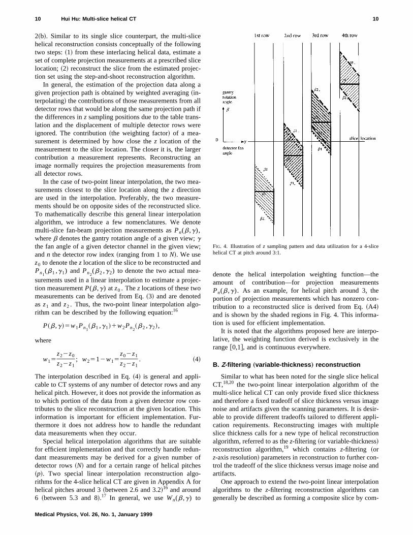
Special helical interpolation algorithms that are suitabfor efficient implementation and that correctly handle redudant measurements may be derived for a given numberdetector rows~N! and for a certain range of helical pitche~p!. Two special linear interpolation reconstruction algorithms for the 4-slice helical CT are given in Appendix A fohelical pitches around 3~between 2.6 and 3.2!16 and around6 ~between 5.3 and 8!.17 In general, we useWn(b,g) to

Medical Physics, Vol. 26, No. 1, January 1999

egalicec-.a

llif

-re

eranm

-

re-ice.onte

w;

d

ec-

-

nys-is

-ant

len-of

s-

r

denote the helical interpolation weighting function—theamount of contribution—for projection measurementsPn(b,g). As an example, for helical pitch around 3, theportion of projection measurements which has nonzero contribution to a reconstructed slice is derived from Eq.~A4!and is shown by the shaded regions in Fig. 4. This information is used for efficient implementation.

It is noted that the algorithms proposed here are interpolative, the weighting function derived is exclusively in therange@0,1#, and is continuous everywhere.

B. Z-filtering „variable-thickness … reconstruction

Similar to what has been noted for the single slice helicaCT,18,20 the two-point linear interpolation algorithm of themulti-slice helical CT can only provide fixed slice thicknessand therefore a fixed tradeoff of slice thickness versus imagnoise and artifacts given the scanning parameters. It is desable to provide different tradeoffs tailored to different appli-cation requirements. Reconstructing images with multipleslice thickness calls for a new type of helical reconstructionalgorithm, referred to as thez-filtering ~or variable-thickness!reconstruction algorithm,19 which containsz-filtering ~orz-axis resolution! parameters in reconstruction to further con-trol the tradeoff of the slice thickness versus image noise anartifacts.

One approach to extend the two-point linear interpolationalgorithms to thez-filtering reconstruction algorithms cangenerally be described as forming a composite slice by com

FIG. 4. Illustration ofz sampling pattern and data utilization for a 4-slicehelical CT at pitch around 3:1.

el

on-y-

ep-

a-ol-

nthe

oraly

ls

-

se

arsehe

eralr-

11 Hui Hu: Multi-slice helical CT 11

bining several slices reconstructed with the two-point lineainterpolation reconstruction algorithm. In implementationthe composite slice can be reconstructed directly withogenerating the original slices. This approach was originaldeveloped for multi-slice CT19 @refer to Eq.~B3! in Appen-dix B# and has been first applied to single slice CT.8,20 Al-ternatively, thez-filtering concept can directly be integratedinto the helical interpolation algorithm, as shown in Appendix B @Eq. ~B4!#.16 The z-filtering reconstruction algorithmallows for interpolation of more than two points.

With thez-filtering reconstruction algorithm, slice profile,image noise, and image artifacts are controlled not only bthe scan parameters~such as helical pitch, beam collimation,and mA!, but also by thez-filtering parameters in reconstruc-tion. Thus, the tradeoff of the slice thickness versus imagnoise and artifacts are no longer fixed for given scanninparameters. They are also controlled by reconstruction prameters. Thez-filtering reconstruction enables users to generate from a single CT scan multiple image sets, representdifferent tradeoffs of the slice thickness, image noise anartifacts to suit for different application requirements.

V. PERFORMANCE OF MULTI-SLICE HELICAL CT

Similar to what has been noted for single slice CT,3,21,5,7

for multi-slice CT, the image quality of the helical CT differsfrom the step-and-shoot CT in terms of the slice profile, image noise, and artifacts. The theoretical models of the sliprofile and image noise of the multi-slice helical CT are developed in Sec. V A. From these theoretical models and computation simulations, slice profile, image noises, and artifacof the 4-slice helical CT are studied and compared witsingle slice helical CT for various helical pitches in Sec. V BThe results are discussed and the volume coverage spperformance of the 4-slice helical CT is also assessed in SV C.

A. Slice profile and noise of multi-slice helical CT:Theoretical models

In this section, we first briefly review the theoreticamodel of the slice profile for single-slice CT. We also provide a new intuitive noise model for single-slice CT. Wethen extend the theoretical models of slice profile and noito multi-slice CT. For simplicity, we only consider the sliceprofile and image noise measured around the axis of rotatio

The slice profile and image noise of single slice CT havbeen modeled theoretically.5,6,21–24We denote the helical in-terpolation weighting function at the center detector chann(g50) as w(b) or w(z). The slice profile, denoted assp(s,d,zs), can be expressed as the following convolution:24

sp~s,d,zs!5E dzb~z!w~z2zs!, ~5a!

whereb(z) is the slice profile of step-and-shoot CT at thesame collimationd and thezs is the distance alongz axis tothe reconstructed slice.

In this paragraph, we present a new intuitive noise modfor the single slice CT, which is derived based on the work

Medical Physics, Vol. 26, No. 1, January 1999

r,utly

-

y

ega--

ingd

-ce--

tsh.eedec.

l-

se

n.e

el

els

of Refs. 21 and 6. We uses0 to denote the noise standarddeviation in the projection data after reconstruction kern~the in-plane filter! is applied. By applying the helicalweighting factor,w(b), the noise standard deviation of theweighted projection becomesw(b)s0 . We further uses todenote the noise measured at the central region of the recstructed image. It follows from the noise propagation analsis that

s25E dbw2~b!s02, ~6!

where the integration is over thoseb wherew(b) is nonzero.Furthermore, we denote the image noise of helical and stand-shoot~axial! CT assH andsA , respectively. For the fullrotation step-and-shoot scan, one hasw(b)5 1

2 for 0<b<2p and therefore from Eq.~6! the image noise issA

2

5(p/2)s02. With other parameters being equal, the noise r

tio of helical to step-and-shoot CT can be expressed as flows:

sH

sA5A2

p E dbw2~b!. ~7a!

It can be proven that this noise model is in good agreemewith the theoretical and experimental results published in tliteratures.3,21,22

The theoretical models of the slice profile and noise fthe multi-slice CT are established with similar mathematicanalyses. Noting that in the multi-slice CT the data macome from different detector rows, Eqs.~5a! and~7a! can beextended for multi-slice CT as follows:

sp~s,d,zs!5E dzb~z! (n51

N

wn~z2zs!, ~5b!

sH

sA5A2

p E db (n51

N

wn2~b!, ~7b!

where,wn(b) or wn(z) stands for the helical interpolationweighting factor at the center detector channel (g50) of thenth detector row. The general slice profile and noise modeof multi-slice CT@Eqs. 5~b! and 7~b!# reduce to the result ofLiang and Kruger10 when the 2-slice CT system is considered.

B. IQ evaluations of the 4-slice helical CT

In this section, we study the IQ~i.e., slice profile, imagenoise, and artifacts! of the 4-slice helical CT for varioushelical pitches. Since different reconstruction algorithmmay result in different slice profiles and image noises, wstudy the thinnest slice profile achievable from the lineinterpolation reconstruction and the lowest image noiachievable at the thinnest slice profile. To be specific, tspecial reconstruction algorithms described in Eqs.~A4! and~A5! were used to study the IQ performance of the 4-slicCT at helical pitches of 3 and 6, respectively. The genealgorithm described in Eq. 4 was used to study IQ perfomance of the 4-slice CT at other helical pitches.

u

e

oot

in

ei-to.1ataeng

menre-

s.

12 Hui Hu: Multi-slice helical CT 12

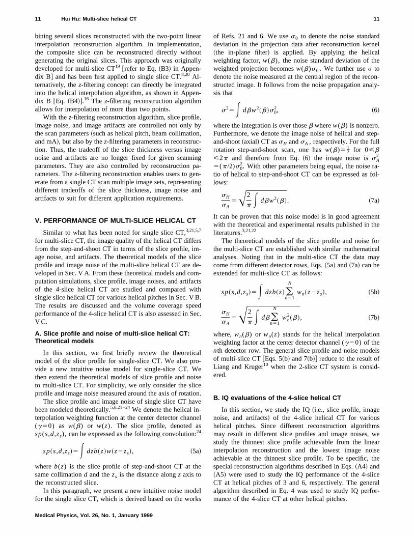
The slice profiles were derived using Eqs.~5a! and ~5b!for the single slice and 4-slice helical CT, respectively. Foprofiles displayed are the single slice CT with helical pitche1 and 2@Fig. 5~a!# and the 4-slice CT with helical pitches 3and 6@Fig. 5~b!#, respectively. From these slice profiles, thratios of helical versus step-and-shoot CT in terms of fuwidth at half-maximum~FWHM! and full width at tenth-maximum~FWTM! are tabulated in Table I and FWHM ra-tios are plotted in Fig. 6~a! for various helical pitches. For

FIG. 5. Slice profiles of~a! the single slice CT with helical pitches 1 and 2and ~b! the 4-slice CT with helical pitches 3 and 6.

TABLE I. Slice profile and noise comparisons~1 vs 4 slice CT!.

Helicalpitch

Single slice CT 4-slice CT

FWHMratio

FWTMratio

Noiseratio

FWHMratio

FWTMratio

Noiseratio

0 1.00 1.00 1.00 1.00 1.00 1.001 1.00 1.56 1.15 1.00 1.56 0.572 1.27 2.23 1.15 1.27 2.23 0.573 1.75 3.00 1.15 1.00 1.56 1.054 2.25 3.82 1.15 1.27 2.23 0.816 3.25 5.52 1.15 1.27 2.23 1.058 4.25 7.27 1.15 1.27 2.23 1.15

Medical Physics, Vol. 26, No. 1, January 1999

rs

ll

each case, the noise ratios of helical versus step-and-shCT were computed using Eqs.~7a! and ~7b! for single sliceand 4-slice helical CT, respectively, and the results areTable I and shown in Fig. 6~b!.

Computer simulations were conducted to study the imagartifacts of both 4-slice and single slice CT systems at varous helical pitches. The distances from the x-ray focal spotthe detector and to the axis of rotation were 94.9 cm and 54cm, respectively. The noises were added to simulate the dacquisition with a constant mA. With reference to Fig. 7, thmathematical phantom used in this study consists of a loelliptical cylinder ~0 HU! simulating the human body, a setof tilted rods~600 HU! at the edge of the elliptical cylindersimulating the ribs, a disk~400 HU! simulating the spin diskand an air cavity~21000 HU! simulating the bowel struc-ture. Figure 7 shows the reconstructed images at the saslice location from two CT systems and with various scaand reconstruction parameters. The images displayed repsent a region of 40326 cm2. The display window is@width,150 HU; level, 0 HU#. The table speed and the FWHM arelisted on the top of each image.

The images in the top two rows in Fig. 7 were from thesingle slice CT system with the x-ray collimation of 2.5 mm

FIG. 6. Plots of the ratios~helical vs axial! of ~a! the slice thickness and~b!the noise of the 4-slice CT versus single slice CT for various helical pitche

13 Hui Hu: Multi-slice helical CT 13

Med

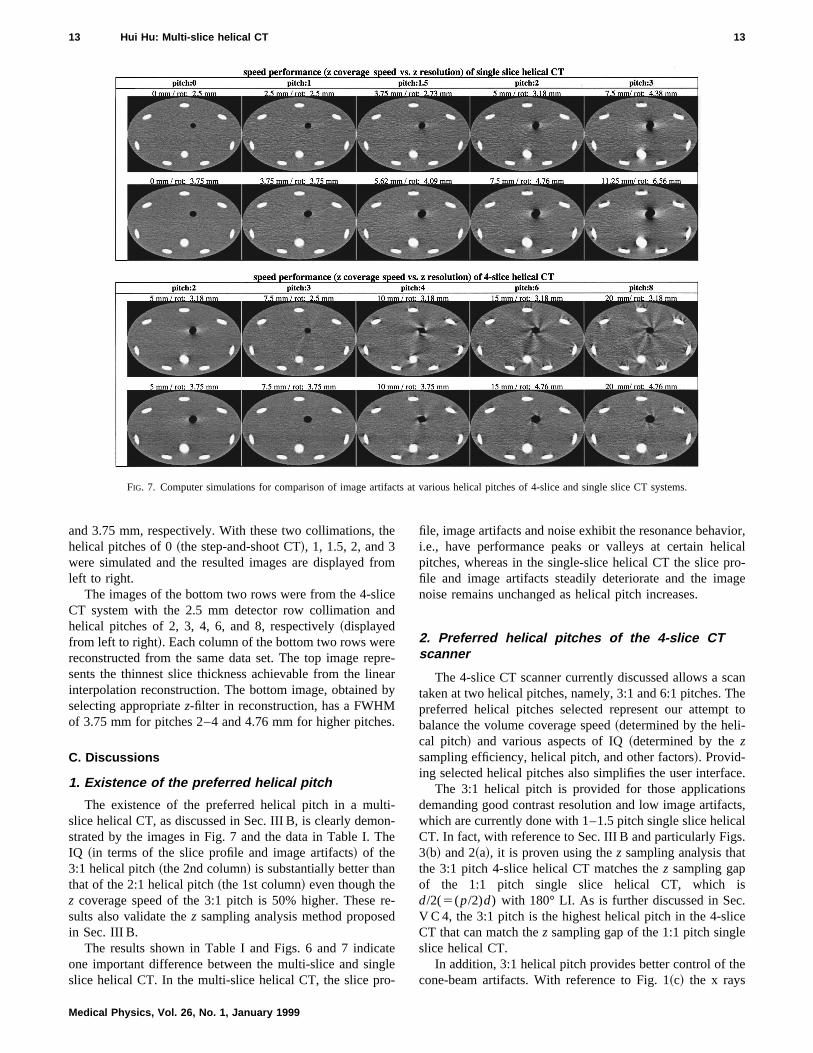
FIG. 7. Computer simulations for comparison of image artifacts at various helical pitches of 4-slice and single slice CT systems.

ior,calro-ge

anhe

t to

ce.sts,al.

.e

e

and 3.75 mm, respectively. With these two collimations, thhelical pitches of 0~the step-and-shoot CT!, 1, 1.5, 2, and 3were simulated and the resulted images are displayed frleft to right.

The images of the bottom two rows were from the 4-slicCT system with the 2.5 mm detector row collimation anhelical pitches of 2, 3, 4, 6, and 8, respectively~displayedfrom left to right!. Each column of the bottom two rows werereconstructed from the same data set. The top image repsents the thinnest slice thickness achievable from the lininterpolation reconstruction. The bottom image, obtainedselecting appropriatez-filter in reconstruction, has a FWHMof 3.75 mm for pitches 2–4 and 4.76 mm for higher pitche

C. Discussions

1. Existence of the preferred helical pitch

The existence of the preferred helical pitch in a multslice helical CT, as discussed in Sec. III B, is clearly demostrated by the images in Fig. 7 and the data in Table I. TIQ ~in terms of the slice profile and image artifacts! of the3:1 helical pitch~the 2nd column! is substantially better thanthat of the 2:1 helical pitch~the 1st column! even though thez coverage speed of the 3:1 pitch is 50% higher. Thesesults also validate thez sampling analysis method proposein Sec. III B.

The results shown in Table I and Figs. 6 and 7 indicaone important difference between the multi-slice and singslice helical CT. In the multi-slice helical CT, the slice pro

ical Physics, Vol. 26, No. 1, January 1999

e

om

ed

re-earby

s.

i-n-he

re-d

tele-

file, image artifacts and noise exhibit the resonance behavi.e., have performance peaks or valleys at certain helipitches, whereas in the single-slice helical CT the slice pfile and image artifacts steadily deteriorate and the imanoise remains unchanged as helical pitch increases.

2. Preferred helical pitches of the 4-slice CTscanner

The 4-slice CT scanner currently discussed allows a sctaken at two helical pitches, namely, 3:1 and 6:1 pitches. Tpreferred helical pitches selected represent our attempbalance the volume coverage speed~determined by the heli-cal pitch! and various aspects of IQ~determined by thezsampling efficiency, helical pitch, and other factors!. Provid-ing selected helical pitches also simplifies the user interfa

The 3:1 helical pitch is provided for those applicationdemanding good contrast resolution and low image artifacwhich are currently done with 1–1.5 pitch single slice helicCT. In fact, with reference to Sec. III B and particularly Figs3~b! and 2~a!, it is proven using thez sampling analysis thatthe 3:1 pitch 4-slice helical CT matches thez sampling gapof the 1:1 pitch single slice helical CT, which isd/2(5(p/2)d) with 180° LI. As is further discussed in SecV C 4, the 3:1 pitch is the highest helical pitch in the 4-slicCT that can match thez sampling gap of the 1:1 pitch singleslice helical CT.

In addition, 3:1 helical pitch provides better control of thcone-beam artifacts. With reference to Fig. 1~c! the x rays

-

e

:1

e-

e

,e

s

ntnte

is,a-

is

t

r

-st

ofge

-l-

dc-

14 Hui Hu: Multi-slice helical CT 14

detected by the 1st and 4th detector rows experience mcone-beam effect than the inner two detector rows, and tare tilted in the opposite directions. At 3:1 helical pitch awith reference to Fig. 3~b!, the measurements derived fromthe 1st and 4th detector rows overlap inz sampling locationsand therefore can be averaged. Thus, the cone beam efof the opposite tilted x rays can be partially canceled. Itnoted that though the data redundancy in general hamthe z coverage speed, some redundancy in this case helpreduce artifacts.

The 6:1 helical pitch is provided for those applicatiodemanding high volume coverage speed and thin slice swhich are currently done with high~around 2:1! pitch singleslice helical CT. It can be proven using thez sampling analy-sis that there are four helical pitches~i.e., pitch 2,4,6 and 8!of the 4-slice helical CT that can match thez sampling gap ofthe 2:1 pitch single slice helical CT, which isd(5(p/2)d)with 180° LI. Although the consideration on thez coveragespeed favors the high pitch~preferably, 8:1 pitch!, the studieson image artifacts~such as the one shown in Fig. 7! indicatethat there are more artifacts near the edge of the 8:1 pimages~the 5th column! than the 6:1 pitch images~the 4thcolumn!. For this reason, the 6:1 pitch is chosen as a pferred tradeoff of thez-coverage speed and image artifacfor this class of applications.

Besides 3:1 and 6:1, other helical pitches~such as 8:1!can be provided in the future for different tradeoffs of thezcoverage speed and various aspects of IQ to suit for diffeapplication requirements.

The 4-slice CT scanner discussed in this paper consista scalable 4-slice detector. To be specific, there are 16 detor cells with 1.25 mm cell size when measured alongz-axis. The detector row collimation can vary from 1.25, 23.75, and 5 mm by selecting electronic switches to combup to 4 individual detector cells in thez direction. With thesefour detector row collimation settings, the two preferred hlical pitches~3:1 and 6:1! translate into eight scan modewhich provide six table translating distances per rotatioThey are 3.75, 7.5, 11.25, 15, 22.5, and 30 mm/rot.

3. Assessment of the volume coverage speedperformance of the 4-slice CT

It is noted from Fig. 5 and Table I that helical pitchesand 6 of the 4-slice CT have similar slice profiles to helicpitches 1 and 2, respectively, of the single slice CT. It is anoted from Table I that the increase of image noise frostep-and-shoot to helical CT is less in the 4-slice CT wpitches 3:1 and 6:1~5%! than in the single slice CT~15%!.The reduction is due to the overlap of the beams defined1st and 4th detector rows when either 360° or 180° periicity is considered.

We assess IQ~in terms of image artifacts and slice thickness! and the volume coverage speed performance of thepitch 4-slice CT relative to the 1:1 pitch single slice CT bcomparing two pairs of the images in the 2nd column of F7. The 2.5 mm image comparison~the 1st versus 3rd row!shows that the 3:1 pitch 4-slice CT can be 3 times as fas

Medical Physics, Vol. 26, No. 1, January 1999

oreheynd

fectsis

perss to

nscan,

itch

re-ts

rent

s oftec-

the.5,ine

e-s,n.

3allsom

ith

byod-

-3:1yig.

t as

the 1:1 pitch single slice CT, with equivalent or slightly moreimage artifacts. On the other hand, the 3.75 mm image comparison ~the 2nd vs 4th row! indicates that the 3:1 pitch4-slice CT can run twice as fast as the 1:1 pitch single slicCT, with less image artifacts.

Similar assessment can be made by comparing the 6pitch 4-slice CT with the 2:1 pitch single slice CT~the 4thcolumn in Fig. 7!. The 3.18 mm image comparison~the 1stvs 3rd row! shows that the 6:1 pitch 4-slice CT can be 3times as fast as the 2:1 pitch single slice CT, with morimage artifacts. On the other hand, the 4.76 mm image comparison ~the 2nd vs 4th row! indicates that the 6:1 pitch4-slice CT can run twice as fast as the 2:1 pitch single slicCT with less image artifacts~i.e., image distortions!.

These studies confirmed thez sample analysis~in the pre-vious section!, proving that 3:1 and 6:1 pitch 4-slice CT canprovide equivalent IQ of 1:1 and 2:1 pitch single slice CTrespectively. Furthermore, they demonstrate that the 4-slichelical CT can provide equivalent IQ at 2 to 3 times thevolume coverage speed of the single slice helical CT.

4. Other discussions

In this paper, we used an intuitive picture of interlacinghelices to illustrate the concept ofz-sampling efficiency andto predict image quality. This is an approximate analysibecause, as shown in Fig. 4 and by Eq.~A3!, a complemen-tary fan-beam projection contains measurements at differez locations and the dashed helices in Figs. 2 and 3 represethez locations of the center detector channel. Although thesvariations can be accounted for by a more rigorous analysinvolving the data sampling diagram such as Fig. 4 and equtions such as~A3!, the study shown in Secs. V B and V Cindicates that this intuitive analysis serves the purpose of thstudy quite well.

With reference to Figs. 2~b! and 3~b! and the discussion inSecs. III B and V C 2, it is further noted that there are tworequirements for achieving thez sampling gap ofd/2 inmulti-slice CT: first, the helical pitch is an odd integer so thathe dashed helices bisect the gaps of the solid helices@referto Fig. 3~b!#; second, the helical pitch is less than the numbeof detector rows so that there is no seam in x-ray beamcoverage after each rotation. These two requirements combined lead to the conclusion that the 3:1 pitch is the highehelical pitch for the 4-slice CT that can match thez samplinggap ofd/2.

To be specific, for 5:1 and 7:1 helical pitches of the4-slice CT, the dashed helices cannot bisect the every gapsthe solid helices because of the seam of x-ray beam coveraafter each rotation.@The case of helical pitch around 5:1 isshown in Fig. 2~b!.# Thus, helical pitches of 5:1 and 7:1result in an uneven sampling pattern,d for certain angularregion andd/2 for the rest. Consequently, the image appearance is relatively unstable, depending on whether the chalenging structure is sampled withd/2 or d spacing, which isdetermined by a clinically uncontrollable parameterb0—thegantry rotation angle when the slice to be reconstructepasses the CT gantry plane. Given the complicated chara

r

leCT

lice

of

e

of

-nn

15 Hui Hu: Multi-slice helical CT 15

teristics of 5:1 and 7:1 helical pitches and the scope of tpaper, we did not include the 5:1 and 7:1 helical pitchesTable I and Fig. 7. This would not affect any discussion aconclusion in this paper. Furthermore, it is noted that theand the volume coverage speed performance of the 1:1 p4-slice CT are similar to a 1:1 pitch single slice CT. Thighlight the key results, the images of the 1:1 pitch 4-slCT are not included in Fig. 7.

Most discussions in this paper, unless specified otherwapply to multi-slice helical CT in general. The general dcussions include the concept of the preferred helical pitchthe general interpolation algorithm, andz-filtering recon-struction@Eqs.~4!, ~B2!–~B4!#, and the theoretical models oslice profile and noise. Furthermore, all the discussionsthis paper, although directly for fan-beam CT geometry, cbe readily extended to the parallel-beam projections eitcollected directly or derived from fan beam projections.particular, the algorithms work with the quarter-detectooffset CT system alignment.

VI. CONCLUSIONS

The scan and reconstruction principles of multi-slice hlical CT have been presented. They include the preferhelical pitch; the helical interpolation algorithms; and thz-filtering reconstruction. The concept of the preferred hecal pitch has been discussed in general with a newly pposedz sampling analysis. The helical interpolation algrithms and the z-filtering reconstructions have beedeveloped for multi-slice CT. The theoretical models of sliprofile and noise have been established for multi-slice helCT. For the 4-slice helical CT in particular, preferred helicpitches have been selected. Special helical interpolationgorithms have been developed. Image quality of the 4-shelical CT have been studied and compared with single shelical CT. The results show that the slice profile, imaartifacts, and noise exhibit performance peaks or valleyscertain helical pitches in multi-slice CT, whereas in singslice CT the image noise remains unchanged and the sprofile and image artifacts steadily deteriorate with increing helical pitch. The study indicates that the 4-slice heliCT can provide equivalent image quality at 2 to 3 times tvolume coverage speed of the single slice helical CT.

ACKNOWLEDGMENTS

The author would like to thank Richard Kinsinger, Norbert Pelc, Armin Pfoh, Carl Crawford, Stan Fox, Sholom Acelsberg, Bob Senzig, Gray Strong, H. David He, GeoSeidenschnur, and Tinsu Pan for their help at different staof this research. The author wishes to express his sinappreciation for the valuable comments and suggestimade by the anonymous associate editor and reviewers.

APPENDIX A: SPECIAL LI ALGORITHMS FOR THE4-SLICE HELICAL CT

In this Appendix, we present special linear interpolatireconstruction algorithms for the 4-slice helical CT at pitcharound 3:116 and 6:1,17 respectively. The four rows of pro

Medical Physics, Vol. 26, No. 1, January 1999

hisin

ndIQitcho

ice

ise,is-es,

fin

anherInr-

e-redeli-ro-o-nceicalalal-

licelicege

atle-lice

as-calhe

-k-rgegescereons

ones-

jection data are illustrated in Fig. 4 in the form of detectofan angle ~the horizontal axis! versus the gantry rotationangle~the vertical axis!. With reference to Fig. 4 and withoutloss of generality, it is assumed that the gantry rotation angequals to 0 when the slice to be reconstructed passes thegantry plane@i.e., b0 in Eq. ~3a! equals to 0#. We usebn todenote the gantry rotation angle when the reconstructed spasses the fan beam defined by thenth detector row. It fol-lows from Eqs.~3! that

bn52Znp/p, ~A1!

where

Z@1 – 4#5@21.5,20.5,0.5,1.5#. ~A2!

The parameterp is the helical pitch. The fan-beam projectionof view bn are shown as the solid lines in Fig. 4. Becausethe z displacement of the multi-slice detector,bn are shiftedfrom one detector row to the next in the direction of thgantry rotation angle. Furthermore, we usebn6 to denote thecomplementary data derived from the fan-beam projectionview bn using the 180° periodicity. It then follows that

bn65bn6p22g52Znp/p6p22g. ~A3!

The relative relationship ofbn and bn6 is shown in Fig. 4for helical pitch around 3:1. We useWn(b,g) to denote thehelical interpolation weighting function—the amount of contribution. From the special interlacing sampling pattershown in Fig. 4, the helical interpolation weighting functiois formulated as follows:

W1~b,g!5a~x1!50 b<b22

b2b22

b12b22

b22,b<b1

b2b32

b12b32

b1,b,b32

0 b>b32

, ~A4.1!

W2~b,g!550 b<b32

b2b32

b22b32

b32,b<b2

U2~b,g!1V2~b,g! b2,b,bM

0 b>bM

, ~A4.2!

where

U2~b,g!5a~x2!50 b<b2

b2b11

b22b11

b2,b,b11

0 b>b11

,

and

16 Hui Hu: Multi-slice helical CT 16

V2~b,g!5~12a~x2!!50 b<b2

b2b42

b22b42

b2,b,b42

0 b>b42

,

W3~b,g!550 b<bm

U3~b,g!1V3~b,g! bm,b<b3

b2b21

b32b21

b3,b,b21

0 b>b21

, ~A4.3!

where

U3~b,g!5a~x2!50 b<b11

b2b11

b32b11

b11,b,b3

0 b>b3

,

and

V3~b,g!5~12a~x2!!50 b<b42

b2b42

b32b42

b42,b,b3

0 b>b3

,

W4~b,g!5~12a~x3!!50 b<b21

b2b21

b42b21

b21,b<b4

b2b31

b42b31

b4,b,b31

0 b>b31

. ~A4.4!

In Eqs. ~A4.3! and ~A4.2!, bM5max(b11,b42

) and bm

5min(b11,b42

). It is noted that because of the redundancbetween the measurements by the 1st and 4th detector rotheir contributions can be combined. The way of combintion is controlled bya(x). a(x)51/2 if they are equallyweighted.

The portions of data which have nonzero contributionthe reconstructed slice can be derived from Eqs.~A4!. Theyare shown by the shaded regions of Fig. 4. This informatiis utilized to achieve fast~pipeline! data processing.

It can be proven that this algorithm is applicable in thfollowing pitch range: 2p/(p22gm),helical pitch,4p/(p12gm), where the 2gm denotes the fan angle.Given that 2gm'p/4 on the scanner being discussed, thalgorithm can be used for a helical pitch range of 2,helical pitch,3.2.

Similarly, a linear interpolation algorithm for the 6:1 pitch4-slice CT can be formulated as follows:

Medical Physics, Vol. 26, No. 1, January 1999

yws,

a-

to

on

e

is.6

W1~b,g!51

2 50 b<b32

b2b32

b12b32

b32,b<b1

b2b2

b12b2b1,b,b2

0 b>b2

, ~A5.1!

W2~b,g!550 b<bm

U2~b,g!1V2~b,g! bm,b<b2

b2b3

b22b3b2,b,b3

0 b>b3

, ~A5.2!

where

U2~b,g!51

2 H 0 b<b1

b2b1

b22b1b1,b,b2

0 b>b2

,

and

V2~b,g!51

2 50 b<b42

b2b42

b22b42

b42,b,b2

0 b>b2

,

W3~b,g!550 b<b2

b2b2

b32b2b2,b<b3

U3~b,g!1V3~b,g! b3,b,bM

0 b>bM

, ~A5.3!

where

U3~b,g!51

2 50 b<b3

b2b11

b32b11

b3,b,b11

0 b>b11

,

and

V3~b,g!51

2 H 0 b<b3

b2b4

b32b4b3,b,b4

0 b>b4

,

-.

of

s

n

t

n-

-

’

-

.

-

-

l

17 Hui Hu: Multi-slice helical CT 17

W4~b,g!51

2 50 b<b3

b2b3

b42b3b3,b<b4

b2b21

b42b21

b4,b,b21

0 b>b21

. ~A5.4!

In Eqs. ~A5.2! and ~A5.3!, bm5min(b1,b42), and bM

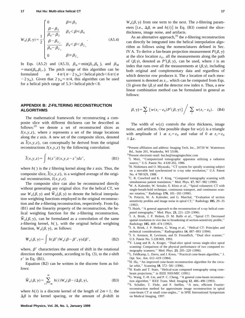
5max(b4,b11). The pitch range of this algorithm can beformulated as 4p/(p22gm),helical pitch,6p/(p22gm). Given that 2gm'p/4, this algorithm can be usedfor a helical pitch range of 5.3,helical pitch,8.

APPENDIX B: Z-FILTERING RECONSTRUCTIONALGORITHMS

The mathematical framework for reconstructing a composite slice with different thickness can be describedfollows:19 we denote a set of reconstructed slices aI (x,y,z), where z represents a set of the image locationalong thez axis. A new set of the composite slices, denoteas I (x,y,z), can conceptually be derived from the originareconstructionsI (x,y,z) by the following convolution:

I ~x,y,z!5E h~z8!I ~x,y,z2z8!dz8, ~B1!

whereh( ) is thez filtering kernel along thez axis. Thus, thecomposite slice,I (x,y,z), is a weighted average of the origi-nal reconstruction,I (x,y,z).

The composite slice can also be reconstructed direcwithout generating any original slice. For the helical CT, wuseWn(b,g) and Wn(b,g) to denote the helical interpola-tion weighting functions employed in the original reconstruction and thez-filtering reconstruction, respectively. From Eq~B1! and the linearity property of the reconstruction, the helical weighting function for thez-filtering reconstruction,Wn(b,g), can be formulated as a convolution of the samz-filtering kernel, h( ), with the original helical weightingfunction,Wn(b,g), as follows:

Wn~b,g!5E h~b8!Wn~b2b8,g!db8, ~B2!

where,b8 characterizes the amount of shift in the rotationadirection that corresponds, according to Eq.~3!, to thez-shiftz8 in Eq. ~B1!.

Equation~B2! can be written in the discrete form as fol-lows:

Wn~b,g!5 (i 52m

m

h~ i !Wn~b2 iDb,g!, ~B3!

whereh( i ) is a discrete kernel of the length of 2m11; theDb is the kernel spacing, or the amount ofb-shift in

Medical Physics, Vol. 26, No. 1, January 1999

-asssdl

tlye

-.-

e

l

Wn(b,g) from one term to the next. Thez-filtering param-eters @i.e., Db, m and h( i )# in Eq. ~B3! control the slice-thickness, image noise, and artifacts.

As an alternative approach,16 thez-filtering reconstructioncan directly be integrated into the helical interpolation algorithm as follows using the nomenclatures defined in SecIV A. To derive a fan-beam projection measurementP(b,g)at the slice locationz0 , all the measurements along the pathof ~b,g!, denoted asPi(b,g), can be used, wherei is anindex that runs over all the measurements at~b,g!, includingboth original and complementary data and regardlesswhich detector row produces it. Thez location of each mea-surement is denoted aszi , which can be computed from Eqs.~3! given the~b,g! and the detector row indexn. Thus, a newlinear combination method can be formulated in general afollows:

b,g)5(i

@w~zi2z0!Pi~b,g!#Y (i

w~zi2z0!. ~B4!

The width of w(z) controls the slice thickness, imagenoise, and artifacts. One possible shape forw(z) is a trianglewith amplitude of 1 atzi5z0 and value of 0 atzi5z0

6Dz.

a!Present affiliation and address: Imaging Tech, Inc., 20720 W. WatertowRd., Suite 201, Waukesha, WI 53186.

b!Present electronic-mail: hui.hu@imagingtechinc.com1I. Mori, ‘‘Computerized tomographic apparatus utilizing a radiationsource,’’ U.S. Patent No. 4 630 202, 1986.

2H. Nishimura and O. Miyazaki, ‘‘CT system for spirally scanning subjecton a movable bed synchronized to x-ray tube revolution,’’ U.S. PatenNo. 4 789 929, 1988.

3C. R. Crawford and K. F. King, ‘‘Computed tomography scanning withsimultaneous patient translation,’’ Med. Phys.17, 967–982~1990!.

4W. A. Kalender, W. Seissler, E. Klotzet al., ‘‘Spiral volumetric CT withsingle-breath-hold technique, continuous transport, and continuous scaner rotation,’’ Radiology176, 181–183~1990!.

5A. Polacin, W. A. Kalender, and G. Marchal, ‘‘Evaluation of sectionsensitivity profiles and image noise in spiral CT,’’ Radiology185, 29–35~1992!.

6J. Hsieh, ‘‘A general approach to the reconstruction of x-ray helical computed tomography,’’ Med. Phys.23, 221–229~1996!.

7J. A. Brink, J. P. Heiken, D. M. Balfeet al., ‘‘Spiral CT: Decreasedspatial resolutionin vivo due to broadening of section-sensitivity profile,’’Radiology185, 469–474~1992!.

8J. A. Brink, J. P. Heiken, G. Wanget al., ‘‘Helical CT: Principles andtechnical considerations,’’ Radiographics14, 887–893~1994!.

9J. S. Arenson, R. Levinson, and D. Freundlich, ‘‘Dual slice scanner,’U.S. Patent No. 5 228 069, 1993.

10Y. Liang and R. A. Kruger, ‘‘Dual-slice spiral versus single-slice spiralscanning: Comparison of the physical performance of two computed tomography scanners,’’ Med. Phys.23, 205–220~1996!.

11L. Feldkamp, L. Davis, and J. Kress, ‘‘Practical cone-beam algorithm,’’ JOpt. Soc. Am. 612–619~1984!.

12H. Hu, ‘‘An improved cone-beam reconstruction algorithm for the circu-lar orbit,’’ Scanning18, 572–581~1996!.

13H. Kudo and T. Stato, ‘‘Helical-scan computed tomography using conebeam projections,’’ in IEEE NSS/MIC~1991!.

14G. Wang, T.-H. Lin, and P. C. Cheng, ‘‘A general cone-beam reconstruction algorithm,’’ IEEE Trans. Med. Imaging12, 486–496~1993!.

15S. Schaller, T. Flohr, and P. Steffen, ‘‘A new, efficient Fourier-reconstruction method for approximate image reconstruction in spiracone-beam CT at small cone-angles.,’’ in SPIE International Symposiumon Medical Imaging, 1997.

f

n-

.

18 Hui Hu: Multi-slice helical CT 18

16H. Hu and N. Pelc, ‘‘Systems, methods, and apparatus for reconstrucimages in a CT system implementing a helical scan,’’ U.S. Patent N5 559 847, 1996.

17H. Hu, ‘‘Image reconstruction for a CT system implementing a four fabeam helical scan,’’ U.S. Patent No. 5 541 970, 1996.

18H. Hu and Y. Shen, ‘‘Helical CT reconstruction with longitudinal filtration,’’ Med. Phys.25, 2130~1998!.

19H. Hu, ‘‘Method and apparatus for multislice helical image reconstructiin a computer tomography system,’’ U.S. Patent No. 5 606 585, 1997

20H. Hu and Y. Shen, ‘‘Helical reconstruction algorithm with userselectable section profile,’’ in RSNA, 189~1996!.

Medical Physics, Vol. 26, No. 1, January 1999

tingo.

n

-

on.-

21W. A. Kalender and A. Polacin, ‘‘Physical performance characteristics ospiral CT scanning,’’ Med. Phys.18, 910–915~1991!.

22G. Wang and M. W. Vannier, ‘‘Helical CT image noise: Analytical re-sults,’’ Med. Phys.20, 1635–1640~1993!.

23G. Wang and M. W. Vannier, ‘‘Longitudinal resolution in volumetricx-ray computerized tomography: Analytical comparison between convetional and helical computerized tomography,’’ Med. Phys.21, 429–433~1994!.

24H. Hu and S. H. Fox, ‘‘The effect of helical pitch and beam collimationon the lesion contrast and slice profile in helical CT imaging,’’ MedPhys.23, 1943–1954~1996!.