Multi-scale methods in quantum field theoryPRD 95,094501 (2017)

Goal: coarse-scale effective field theory

W. N. Polyzou, Tracie Michlin and Fatih Bulut

The University of Iowa (WP and TM),Inonu University (FB)

Outline / Strategy

• Construct a multi-resolution (wavelet) basis.

• Exactly decompose fields into discrete degrees offreedom with different resolutions.

• Perform resolution and volume truncations on the fields.

• Use the truncated fields to construct a truncatedHamiltonian.

• Block diagonalize the truncated Hamiltonian byresolution.

• Evolve fields with coarse-scale block Hamiltonian.

• Construct the vacuum and correlation functions.

Comments

• The block diagonalization eliminates the short distancedegrees of freedom.

• The effects of the short distance degrees of freedom arereplaced by new coarse scale effective interactions.

• The truncated problem can be formulated in thetruncated field fock representation, with vacuum definedby an|0〉 = 0

Basis construction (Daubechies wavelets)

Generated by the fixed point, s(x), of arenormalization group equation

s(x) = D (2K−1∑l=0

hlTls(x))︸ ︷︷ ︸

block average︸ ︷︷ ︸rescale

.

Unitary translations Unitary scale transformations

Ts(x) = s(x − 1) Ds(x) =√

2s(2x).

Scale fixing (RG equation homogeneous)∫dxs(x) = 1

Weights hl (constants) determine properties of basis

Table: Filter weights for Daubechies K=3 Wavelets

h0 (1 +√10 +

√5 + 2

√10 )/16

√2

h1 (5 +√10 + 3

√5 + 2

√10 )/16

√2

h2 (10− 2√10 + 2

√5 + 2

√10 )/16

√2

h3 (10− 2√10− 2

√5 + 2

√10 )/16

√2

h4 (5 +√10− 3

√5 + 2

√10 )/16

√2

h5 (1 +√10−

√5 + 2

√10 )/16

√2

Determined uniquely (up to reflection) by requiring s(x) and s(x − n)are orthonormal and degree 2 polynomials in x can be point-wiseexpressed as linear combinations of the s(x − n).

Scaling functions, skn (x)

Translate and rescale the fixed point, s(x)

skn (x) := DkT ns(x) = 2k/2s(

2k(x − 2−kn)).

Sk := {f (x)|f (x) =∞∑

n=−∞cns

kn (x),

∞∑n=−∞

|cn|2 <∞}.

Sk := resolution 2−k subspace, {skn (x)} basis

Sk := DkS0

Sk ⊂ Sk+n n ≥ 0

Sk+1 = Sk ⊕Wk Wk 6= {∅}.

Multi-resolution decomposition of Hilbert space

Sk+1 = Sk ⊕Wk

L2(R) = Sk ⊕Wk ⊕Wk+1 ⊕Wk+2 ⊕Wk+3 ⊕ · · · =

· · · ⊕Wk−2 ⊕Wk−1 ⊕Wk ⊕Wk+1 ⊕Wk+2 ⊕ · · ·

Wavelets (basis for Wk)

w(x) := D

(2K−1∑l=0

glTls(x)

)gl = (−)lh2K−1−l

wkn (x) := DkT nw(x) = 2k/2w

(2k(x − 2−kn)

).

Multi-resolution basis

{ξm(x)} = {skn (x)}∞n=−∞ ∪ {w ln(x)}∞n=−∞∞l=k

• Complete, orthonormal

• Limited smoothness (increases with K)

• Compact support (skn (x),wkn (x)) ⊂ 2−k [n, n + 2K − 1]

• skn (x) resolution 2−k , w ln(x) resolution 2−l+1 not in 2−l

• xn =∑

m cmskm(x) (pointwise, n < K)

•∫dxxmw l

n(x) = 0, m < K

• Basis functions are fractal

Multi-resolution decomposition of canonical fields

ξn(x) ∈ {skn (x),w ln(x)} ξn(x) := ξn1(x)ξn2(y)ξn3(z)

Φ(x, t) =∑

n

Φk(n, t)ξn(x) Φk(n, t) =

∫dxξn(x)Φ(x, t)

Π(x, t) =∑

n

Πk(n, t)ξn(x) Πk(n, t) =

∫dxξn(x)Π(x, t)

[Φ(n, t),Π(m, t)] = iδn,m

[Φ(n, t),Φ(m, t)] = [Π(n, t),Π(m, t)] = 0,

Light front!

[Φlf (m),Φlf (n)] =

∫ξm(x)Dpj(x− y)ξn(y)dxdy := Dpj

mn

Dpjmn =

∫ξm(x)

1

2πε(x− − y−)δ((x⊥ − y⊥)2)ξn(y)

Vacuum = Fock vacuum

• The expansion is exact.

• Operator valued distributions are replaced by infinitesums of well-defined discrete field operators.

• Products of discrete the fields are well defined.

• Discrete fields satisfy canonical commutation relations(or light-front commutation relations).

• Decomposes the field into local observables byresolution.

• Natural resolution (limit l) and volume (limit n)truncations. on

• Because this is an exact representation of the fields:

• The multiresolution decomposition can be used in anyfield-theoretic application.

• The expansion can be used in perturbation theory.

• The discrete fields can be used in Hamiltonians,Lagrangians or path integrals.

• Light-front multi-resolution representation of thedynamics can be constructed.

• Integrals on free field Wightman functions exist - exactdistrubutions recovered in the volume/resolution limit.

Resolution and volume truncated fields

ΦT (x, t) =∑n∈I

Φk(n, t)ξn(x)

ΠT (x, t) =∑n∈I

Πk(n, t)ξn(x)

• Restrict the index set to a finite subset, I (finitevolume, finite resolution).

• Truncated fields are still differentiable functions of x

I = {k ≤ l ≤ lmax ,−nl ,max ≤ nl ≤ nl ,max}

Hamiltonians (exact multi-scale representation)

Mass and kinetic terms

µ2∫

dxΦ2(x, t) = µ2∑

Φ(m, t)2∫

dxΠ2(x, t) =∑

Π(m, t)2

Derivative terms∫dx∇∇∇Φ(x, t) · ∇∇∇Φ(x, t) =

∑Φ(m, t)DmnΦ(n, t)

Dmn :=

∫dx∇∇∇ξm(x) · ∇∇∇ξn(x)

Local interactions∫dxΦN(x, t) =

∑Γn1···nN

Φ(n1, t) · · ·Φ(nN , t)

Γn1···nN=

∫dxξn1(x) · · · ξnN

(x)

Terms almost local due to support conditions

All coefficients can be computed analytically using therenormalization group equation, scale fixing condition, and

weight coefficients, hl . For example the non-zero matrixelements

D0mn :=

∫ds0m(x)

dx

ds0n(x)

dxdx

have the following exact rational values

D0s;40 = D0

s;−40 = −3/560

D0s;30 = D0

s;−30 = −4/35

D0s;20 = D0

s;−20 = 92/105

D0s;10 = D0

s;−10 = −356/105

D0s;00 = 295/56.

Truncated Hamiltonian(replace fields by truncated fields)

Dynamics

Φn(t) = i [HT ,Φn(t)] Πn(t) = i [HT ,Πn(t)]

Initial conditions

[Φ(n, 0),Π(m, 0)] = iδn,m

[Φ(n, 0),Φ(m, 0)] = [Π(n, 0),Π(m, 0)] = 0,

Hilbert space - the truncated problem well-defined in thefree field Fock space

a(n) :=1√2

(Φ(n, 0) + iΠ(n, 0)) [a(n)a†(m)] = δm,n

Advantage of wavelet basis

Scaling properties of coefficients (dim = 1 + 1)

Sk+m = Sk ⊕Wk ⊕ · · · ⊕Wk+m

∑DkmnΦk

mΦkn = 22k

∑D0mnΦk

mΦkn

and

∑Γkn+1···nN Φk

n1 · · ·ΦknN

= 23k(n2−1)∑

Γ0n+1···nN Φk

n1 · · ·ΦknN

⇓

Operator renormalization group equation relates infinitevolume H truncated at different scales (rescale + canonical

transformation)

Hk(Φk ,Πk , µ2(k), γN(k)) = 2kH0(Φ0,Π0, 2−2kµ2(0), 2k(N−4)γN(0))

Canonical transformation Resolution and volume

Φk = ηΦ0 Πk = η−1Π0 η = 2−k/2

Problem: Construct a coarse-scale effective theory thatincludes the effects of eliminated fine-scale degrees of

freedom. First test: Free field theory in 1+1 dimension.

H =1

2

∫(Π(x , 0)Π(x , 0)+∇∇∇Φ(x , 0)·∇∇∇Φ(x , 0)+µ2Φ(x , 0)Φ(x , 0))dx ,

Spatial derivatives give non-trivial scale coupling

Hk+nTs = Hk

Ts + HTw + HTsw

• Resolution 1/2n+k Hamiltonian = resolution 1/2k

Hamiltonian + fine scale corrections + scale couplingterms

• Goal - block diagonalize truncated Hamiltonian byresolution

HkT :=

1

2(∑n

Πk(s, n, 0)Πk(s, n, 0)+∑mn

Φk(s,m, 0)Dks;mnΦk(s, n, 0)

+µ2∑n

Φk(s, n, 0)Φk(s, n, 0)),

Hw :=1

2(∑n,l

Πl(w , n, 0)Πl(w , n, 0)+∑

m,l ,n,j

Φl(w ,m, 0)D ljw ;mnΦj(w , n, 0)

+µ2∑l ,n

Φl(w , n, 0)Φl(w , n, 0)),

Hsw :=1

2

∑m,l ,n

Φl(w ,m, 0)D lksw ;mnΦk(s, n, 0).

Use similarity renormalization group evolution to decouplescales (eliminate D lk

sw ;mn)

Generate unitarily equivalent Hamiltonians

H(λ) = U(λ)H(0)U†(λ)

dU(λ)

dλ=

dU(λ)

dλU†(λ)U(λ) = K (λ)U(λ)

K (λ) =dU(λ)

dλU†(λ) = −K †(λ)

Use a generator K (λ) of the form

K (λ) = [G (λ),H(λ)]

dH(λ)

dλ= [K (λ),H(λ)] = [[G (λ),H(λ)],H(λ)] = [H(λ), [H(λ),G (λ)]]

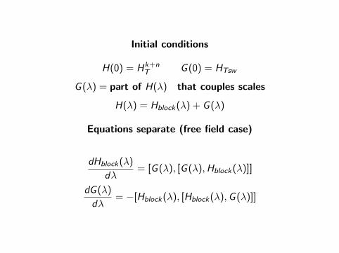
Initial conditions

H(0) = Hk+nT G (0) = HTsw

G (λ) = part of H(λ) that couples scales

H(λ) = Hblock(λ) + G (λ)

Equations separate (free field case)

dHblock(λ)

dλ= [G (λ), [G (λ),Hblock(λ)]]

dG (λ)

dλ= −[Hblock(λ), [Hblock(λ),G (λ)]]

Expand the first equation in basis of eigenstates ofHC := G (λ), the second in eigenstates of HB := Hblock(λ)

dHBmn(λ)

dλ= (ecm(λ)− ecn(λ))2HBmn(λ)

anddHCmn(λ)

dλ= −(ebm(λ)− ebn(λ))2HCmn(λ).

Integrating

HBmn(λ) = e∫ λ0 (ecm(λ′)−ecn(λ′))2dλ′HBmn(0)

HCmn(λ) = e−∫ λ0 (ebm(λ

′)−ebn(λ′))2dλ′HCmn(0).

• Formal solution shows coupling terms exponentiallysuppressed.

• Evolves to decoupled effective Hamiltonians involvingdegrees of freedom on different scales.

• Can stall when eigenvalues get close or cross.

• The choice of generator is specific to the free field case.

• Evolution easily computed - Hamiltonian has discretecanonical fields with known constant coefficients.

• Free field case allows a detailed analysis of the evolutionof scales.

Test case: 16 scaling functions, 16 wavelets, BC - vanish atboundary

H(λ) has 16 quadratic types obtained by taking products ofΦs(n, 0), Πs(m, 0), Φw (n, 0), and Πw (m, 0).

H(λ) =∑mn

cswmn(λ)Φs(m, 0)Φw (n, 0) + · · ·

The λ evolution should drive the coefficients cswmn(λ) of theproducts Φs(n, 0)Φw (m, 0), · · · to 0.

Plots show the Hilbert-Schmidt norms of the coefficientmatrices of each type of operator as a function of λ.

13.7

13.8

13.9

14

14.1

14.2

14.3

14.4

0 5 10 15 20

HS n

orm

λ

Φ scale - Φ scale

0 0.2 0.4 0.6 0.8

1 1.2 1.4 1.6 1.8

0 5 10 15 20

HS n

orm

λ

Φ scale - Φ wavelet

0 0.2 0.4 0.6 0.8

1 1.2 1.4 1.6 1.8

0 5 10 15 20

HS n

orm

λ

Φ wavelet - Φ scale

81.04 81.06 81.08

81.1 81.12 81.14 81.16 81.18

81.2 81.22 81.24

0 5 10 15 20

HS n

orm

λ

Φ wavelet - Φ wavelet

0 16 32 48

0

16

32

48

λ= 0. 0, mass=1.0

0.0

0.5

1.0

1.5

2.0

2.5

3.0

3.5

4.0

4.5

5.0

Figure: Full matrix, λ=0,mass=1

0 16 32 48

0

16

32

48

λ= . 2, mass=1.0

0.0

0.5

1.0

1.5

2.0

2.5

3.0

3.5

4.0

4.5

5.0

Figure: Full matrix, λ=0.2,mass=1

0 16 32 48

0

16

32

48

λ= 2. 0, mass=1.0

0.0

0.5

1.0

1.5

2.0

2.5

3.0

3.5

4.0

4.5

5.0

Figure: Full matrix, λ=2.0,mass=1

0 16 32 48

0

16

32

48

λ= 20. 0, mass=1.0

0.0

0.5

1.0

1.5

2.0

2.5

3.0

3.5

4.0

4.5

5.0

Figure: Full matrix, λ=20.0,mass=1

Observations / Questions?

• Coefficients exhibit expected behavior.

• The decay of the coefficients of the scale coupling termsis initially fast, but slows significantly.

• Truncated free fields are equivalent to coupledoscillators; how does the SRG evolution distribute thenormal modes among the blocks?

To get a more detailed understanding of the effects of the λflow note that the truncated Hamiltonian has the form

HT =1

2[(Πs ,Πw )

(Is 00 Iw

)(Πs

Πw

)+

(Φs ,Φw )

(µ2I + Ds Dsw

Dws µ2I + Dw

)(Φs

Φw

)]

M :=

(µ2I + Ds Dsw

Dws µ2I + Dw

)OtMO =

(ms 00 mw

)where ms and mw are diagonal matrices consisting of

eigenvalues of the matrix M.

Transformed discrete fields are related by the canonicaltransformation(

Φ′s

Φ′w

):= Ot

(Φs

Φw

)and

(Π′s

Π′w

):= Ot

(Πs

Πw

).

H ′ = UHU† =1

2[(Π′s ,Π′w )

(I 00 I

)(Π′s

Π′w

)+

(Φ′s ,Φ′w )

(ms 00 mw

)(Φ′s

Φ′w

)]

• Transformed Hamiltonian is the Hamiltonian foruncoupled harmonic oscillators with frequencies

√mi

• ΠΠ coefficients in flow-evolved Hamiltonian areapproximately (1/2)(Is ⊕ Iw ) so √ of eigenvalues of Mcorrespond to normal mode frequencies.

• A general O will separate the eigenvalues of M into twodistinct groups - there is no general relation betweennormal mode frequencies and scale.

Table: Normal mode frequencies

λ = 20, µ = 1 truncated exact 1:16 exact 17:32

1.037e+00 1.037e+00 1.041e+00 1.665e+011.145e+00 1.146e+00 1.153e+00 1.925e+011.326e+00 1.333e+00 1.340e+00 2.208e+011.583e+00 1.609e+00 1.604e+00 2.512e+011.919e+00 1.995e+00 1.947e+00 2.834e+012.341e+00 2.525e+00 2.373e+00 3.167e+012.861e+00 3.236e+00 2.890e+00 3.507e+013.493e+00 4.161e+00 3.508e+00 3.846e+014.263e+00 5.317e+00 4.243e+00 4.178e+015.201e+00 6.689e+00 5.112e+00 4.495e+016.346e+00 8.232e+00 6.134e+00 4.789e+017.722e+00 9.859e+00 7.332e+00 5.053e+019.309e+00 1.145e+01 8.729e+00 5.279e+011.102e+01 1.289e+01 1.034e+01 5.462e+011.274e+01 1.403e+01 1.219e+01 5.597e+011.435e+01 1.476e+01 1.429e+01 5.679e+01

The table shows that the SRG flow equation puts the lowestnormal modes in coarse scale Hamiltonian and the highest

normal mode frequencies in the fine scale Hamiltonian

Observations

• Flow equation methods with a suitable generator can beused to construct an effective field theory with coarsescale degrees of freedom.

• The generator used separates both energy and distancescales.

• Increasing the truncated volume generates new lowfrequency modes, while increasing the resolution addsnew higher frequency normal modes. The mass sets alower bound on the normal mode frequencies.

• The evolved effective Hamiltonian was approximatelylocal.

• The flow equation also exhibited convergence for bothhigher masses and zero mass.

Outlook

• Singh and Brennan (Arxiv 1606:050686) showed thatthe truncated correlation functions converge to theexact free-field Wightman functions.

• The spectral properties suggest that in order to approachthe continuous spectrum of the exact H, the volume andresolution truncations need to be removed together.

• The convergence of the flow equation will slow down asthe separation between normal modes decreases. Thissuggests that the large volume limit will be difficult.

• In interacting theories integrating the flow equationgenerates infinite numbers of operators. Irrelevantoperators need to be identified and eliminated.

• Solution of Heisenberg equations of motion + groundstate can be used to construct space-real-timecorrelation functions as functions of continuous variables.

Next steps

• Study scaling properties of generated inteactions usingthe renormalization group equations to identify thedominant interactions.

• Study implementation of local gauge invariance and theYang Mills limit.

• Study restoration of Poincare symmetry using partitionof unity property.

• Representation of Wilson loops?

• Operator flow equations with interactions ?

1.935

1.94

1.945

1.95

1.955

1.96

1.965

0 5 10 15 20

HS n

orm

λ

Π scale - Π scale

0

0.02

0.04

0.06

0.08

0.1

0.12

0.14

0 5 10 15 20

HS n

orm

λ

Π scale - Π wavelet

0

0.02

0.04

0.06

0.08

0.1

0.12

0.14

0 5 10 15 20

HS n

orm

λ

Π wavelet - Π scale

2.045

2.05

2.055

2.06

2.065

2.07

0 5 10 15 20

HS n

orm

λ

Π wavelet - Π wavelet

0 16 32 48

0

16

32

48

λ= . 2, mass=0.0

0.0

0.5

1.0

1.5

2.0

2.5

3.0

3.5

4.0

4.5

5.0

Figure: Full matrix, λ=0.2,mass=0

0 16 32 48

0

16

32

48

λ= 2. 0, mass=0.0

0.0

0.5

1.0

1.5

2.0

2.5

3.0

3.5

4.0

4.5

5.0

Figure: Full matrix, λ=2.0,mass=0

0 16 32 48

0

16

32

48

λ= . 2, mass=4.0

0.0

0.5

1.0

1.5

2.0

2.5

3.0

3.5

4.0

4.5

5.0

Figure: Full matrix, λ=0.2,mass=4

0 16 32 48

0

16

32

48

λ= 2. 0, mass=4.0

0.0

0.5

1.0

1.5

2.0

2.5

3.0

3.5

4.0

4.5

5.0

Figure: Full matrix, λ=2.0,mass=4