Multi-Objective Optimization of Next-Generation Aircraft ...

Multi-Objective Optimization of Next-Generation

Aircraft Collision Avoidance Software

by

John R. LepirdB.S. Operations ResearchB.S. Mathematical Sciences

United States Air Force Academy (2013)Submitted to the Operations Research Center

in partial fulfillment of the requirements for the degree ofMaster of Science

at theMASSACHUSETTS INSTITUTE OF TECHNOLOGY

June 2015This material is declared a work of the U.S. Government and is not

subject to copyright protection in the United States.

Author . . . . . . . . . . . . . . . . . . . . . . . . . . . . . . . . . . . . . . . . . . . . . . . . . . . . . . . . . . . . . .Operations Research Center

May 15, 2015

Certified by. . . . . . . . . . . . . . . . . . . . . . . . . . . . . . . . . . . . . . . . . . . . . . . . . . . . . . . . . .Michael P. Owen

Technical Staff, Lincoln LaboratoryThesis Supervisor

Certified by. . . . . . . . . . . . . . . . . . . . . . . . . . . . . . . . . . . . . . . . . . . . . . . . . . . . . . . . . .Dimitri P. Bertsekas

McAfee Professor of EngineeringThesis Supervisor

Accepted by . . . . . . . . . . . . . . . . . . . . . . . . . . . . . . . . . . . . . . . . . . . . . . . . . . . . . . . . .Dimitris Bertsimas

Boeing Professor of Operations ResearchCo-Director, Operations Research Center

Disclaimer: The views expressed in this thesis are those of the author and do not

reflect the official policy or position of the United States Air Force, Department of

Defense, or the U.S. Government.

3

Multi-Objective Optimization of Next-Generation Aircraft

Collision Avoidance Software

by

John R. Lepird

Submitted to the Operations Research Centeron May 15, 2015, in partial fulfillment of the

requirements for the degree ofMaster of Science

Abstract

Developed in the 1970’s and 1980’s, the Traffic Alert and Collision Avoidance System(TCAS) is the last safety net to prevent an aircraft mid-air collision. AlthoughTCAS has been historically very effective, TCAS logic must adapt to meet the newchallenges of our increasingly busy modern airspace. Numerous studies have shownthat formulating collision avoidance as a partially-observable Markov decision process(POMDP) can dramatically increase system performance. However, the POMDPformulation relies on a number of design parameters—modifying these parameterscan dramatically alter system behavior. Prior work tunes these design parameterswith respect to a single performance metric. This thesis extends existing work tohandle more than one performance metric. We introduce an algorithm for preferenceelicitation that allows the designer to meaningfully define a utility function. Wealso discuss and implement a genetic algorithm that can perform multi-objectiveoptimization directly. By appropriately applying these two methods, we show thatwe are able to tune the POMDP design parameters more effectively than existingwork.

Thesis Supervisor: Michael P. OwenTitle: Technical Staff, Lincoln Laboratory

Thesis Supervisor: Dimitri P. BertsekasTitle: McAfee Professor of Engineering

Acknowledgments

I would like to thank the MIT Lincoln Laboratory for not only supporting my educa-tion and research over the past two years, but also providing a fantastic environmentfor me to develop as a student, an Air Force officer, and a person. Col (ret.) JohnKuconis was instrumental in bringing me to the lab and to MIT, and for that I amincredibly grateful.

Specifically, I am thankful for the opportunity to work with all my friends andcolleagues in Group 42. I would like to thank Dr. Wesley Olson for his continualleadership and support of my endeavors. This work would not be the same wereit not for the technical guidance and support of Robert Klaus, Ted Londer, JessicaHolland, and Barbara Chludzinski. I am also grateful for the support and friendshipof Robert Moss, Brad Huddleston, Rachel Tompa, and Nick Monath.

I would also like to thank my adviser, Professor Dimitri Bertsekas, for keeping meon track and ensuring that I got the full “MIT experience.” His superlative technicaladvice was also very much appreciated.

I am incredibly thankful for the help of Professor Mykel Kochenderfer. His contin-ual support and technical guidance were invaluable to this effort. Similarly, I cannotthank Dr. Michael Owen enough for his guidance during my entire time at the LincolnLab: his guidance saved me from numerous pitfalls and was instrumental in makingmy research both fruitful and enjoyable.

Finally, I would like to thank all my friends and colleagues at the MIT OperationsResearch Center for their help and insights into this work, as well as their friendship.Although this list is far from incomplete, I would specifically like to thank Zeb Hanley,Kevin Rossillon, Dan Schonfeld, Mapi Testa, and Mallory Sheth — my experience atMIT would not have been the same without you.

This work was sponsored by the FAA TCAS Program Office AJM-233, and Igratefully acknowledge Mr. Neal Suchy for his leadership and support. Interpreta-tions, opinions, and conclusions are those of the authors and do not reflect the officialposition of the United States Government. This thesis leverages airspace encountermodels that were jointly sponsored by the U.S. Federal Aviation Administration, theU.S. Air Force, and the U.S. Department of Homeland Security.

THIS PAGE INTENTIONALLY LEFT BLANK

8

Contents

1 Introduction 15

1.1 Contributions and Outline . . . . . . . . . . . . . . . . . . . . . . . . 16

2 Background 19

2.1 Aircraft Collision Avoidance . . . . . . . . . . . . . . . . . . . . . . . 19

2.2 Partially Observable Markov Decision Processes . . . . . . . . . . . . 21

2.3 Surrogate Modelling . . . . . . . . . . . . . . . . . . . . . . . . . . . 23

2.3.1 Constructing a Surrogate Model . . . . . . . . . . . . . . . . . 24

2.3.2 Exploiting a Surrogate Model . . . . . . . . . . . . . . . . . . 27

3 Preference Elicitation 33

3.1 Introduction . . . . . . . . . . . . . . . . . . . . . . . . . . . . . . . . 33

3.2 Literature Review . . . . . . . . . . . . . . . . . . . . . . . . . . . . . 35

3.2.1 Linear Programming Methods . . . . . . . . . . . . . . . . . . 37

3.2.2 Bayesian Methods . . . . . . . . . . . . . . . . . . . . . . . . . 41

3.3 Our Method . . . . . . . . . . . . . . . . . . . . . . . . . . . . . . . . 43

3.3.1 Model . . . . . . . . . . . . . . . . . . . . . . . . . . . . . . . 44

3.3.2 Inference . . . . . . . . . . . . . . . . . . . . . . . . . . . . . . 45

3.3.3 Query Generation . . . . . . . . . . . . . . . . . . . . . . . . . 53

3.4 Results . . . . . . . . . . . . . . . . . . . . . . . . . . . . . . . . . . . 55

3.4.1 Proof of Concept . . . . . . . . . . . . . . . . . . . . . . . . . 55

3.4.2 Application to Aircraft Collision Avoidance . . . . . . . . . . 61

3.5 Discussion . . . . . . . . . . . . . . . . . . . . . . . . . . . . . . . . . 66

9

4 Multi-Objective Optimization 67

4.1 Background . . . . . . . . . . . . . . . . . . . . . . . . . . . . . . . . 67

4.2 Traffic Alert Optimization . . . . . . . . . . . . . . . . . . . . . . . . 69

4.2.1 Traffic Alert Mechanism . . . . . . . . . . . . . . . . . . . . . 70

4.2.2 Optimization . . . . . . . . . . . . . . . . . . . . . . . . . . . 72

4.2.3 Results . . . . . . . . . . . . . . . . . . . . . . . . . . . . . . . 74

4.3 Discussion . . . . . . . . . . . . . . . . . . . . . . . . . . . . . . . . . 80

5 Conclusion 81

5.1 Summary . . . . . . . . . . . . . . . . . . . . . . . . . . . . . . . . . 81

5.2 Further Work . . . . . . . . . . . . . . . . . . . . . . . . . . . . . . . 82

10

List of Figures

2-1 Example TA display and annunciation. . . . . . . . . . . . . . . . . . 20

2-2 Example RA display and annunciation. . . . . . . . . . . . . . . . . . 20

2-3 Fit of a surrogate model to ACAS data. . . . . . . . . . . . . . . . . 28

2-4 A simple surrogate model vs. reality . . . . . . . . . . . . . . . . . . 29

3-1 Spectrum of preference elicitation methods. . . . . . . . . . . . . . . . 37

3-2 A typical convergence pattern for linear programming formulations. . 40

3-3 A factor graph for our model of preference realization. . . . . . . . . . 44

3-4 Region for which Equation 3.8 is true. . . . . . . . . . . . . . . . . . 46

3-5 Correspondence between loss in utility L and error angle θ for a circular

design set. . . . . . . . . . . . . . . . . . . . . . . . . . . . . . . . . . 57

3-6 Mean loss as a function of preferences given from an infallible expert. 58

3-7 Mean loss as a function of preferences given from a fallible expert. . . 60

3-8 Our Small-Scale Optimization Test. . . . . . . . . . . . . . . . . . . . 63

3-9 Distribution of solutions found with and without preference elicitation.

The base 50 samples are omitted. . . . . . . . . . . . . . . . . . . . . 63

4-1 Utility function optimization on the Pareto front. . . . . . . . . . . . 68

4-2 Traffic alert Pareto front. . . . . . . . . . . . . . . . . . . . . . . . . . 75

4-3 Traffic Alert policy plot for original logic. . . . . . . . . . . . . . . . . 76

4-4 Traffic Alert policy plot for modified OR logic. . . . . . . . . . . . . . 78

4-5 Pareto Front after Logic Change. . . . . . . . . . . . . . . . . . . . . 79

4-6 Distribution of time difference between TA and RA after logic change.

The vertical bar at six seconds is the threshold for a surprise RA. . . 80

11


12

List of Tables

3.1 Description of the four algorithms tested. . . . . . . . . . . . . . . . . 58

3.2 Pairwise statistical comparison tests for best performing algorithms

with an infallible expert. . . . . . . . . . . . . . . . . . . . . . . . . . 59

3.3 Pairwise statistical comparison tests for best performing algorithms

with a fallible expert. . . . . . . . . . . . . . . . . . . . . . . . . . . . 60

3.4 Weights before and after preference elicitation. . . . . . . . . . . . . . 63

3.5 Effect of preference elicitation on collision avoidance optimization. . . 65

4.1 Comparison of TCAS and ACAS traffic alert performance. . . . . . . 78

13


14

Chapter 1

Introduction

The Traffic Alert and Collision Avoidance System (TCAS) is the last safety net for

avoiding an airborne collision. Mandated on all large aircraft flying in United States

and European Union airspace, TCAS monitors the airspace surrounding the airplane

and alerts the pilot of incoming traffic. If necessary, TCAS then instructs the pilots

how to maneuver in order to avoid an impending collision.

Although very effective, TCAS logic is nearly thirty years old. Advances in com-

puter hardware and artificial intelligence have led to development of a next-generation

aircraft collision avoidance system, dubbed the Experimental Aircraft Collision Avoid-

ance System (ACAS-X). Although ACAS-X has shown itself capable of across-the-

board improvement over the existing TCAS system, development is still underway.

One aspect under development is changing certain parameters of ACAS-X to generate

ideal performance.

Optimizing ACAS-X performance with respect to these parameters is very diffi-

cult. First, evaluating its performance can only be accomplished through extensive

simulation: a computational challenge in and of itself. Second, to exacerbate matters,

there is no single metric that completely summarizes “good” performance. One could

simply use the number of near mid-air collisions, but optimizing only this metric

would result in a logic that alerts pilots too frequently to be useful.

The problem of performance evaluation was largely solved by Kyle Smith in his

Master’s thesis[71] by using a machine learning technique known to engineers as

15

“surrogate modelling”[33]. This thesis focuses on the second problem: designing a

complex system subject to multiple conflicting optimization criteria.

1.1 Contributions and Outline

This thesis offers two important contributions to the development of a next-generation

aircraft collision avoidance system:

We develop a novel approach to preference elicitation for engineering design

optimization, allowing experts to meaningfully define a utility function by using

pairwise comparisons between designs. We empirically show that this algorithm

converges faster than existing algorithms to an expert’s true utility function.

We then demonstrate the usefulness of this approach by using it to incorporate

preferences from aviation experts around the world into an optimization of

ACAS-X. Experimental results indicate that the algorithm effectively captured

the experts intent and resulted in a solution better tailored to their needs.

We exploit properties of a certain behavior in the collision avoidance system

to allow us to use a genetic algorithm designed to identify the Pareto frontier

of this behavior. By identifying the frontier directly, we identify a major op-

portunity for improvement in the collision avoidance system. We then show

that exploiting this opportunity results in across-the-board improvement for

this aspect of aircraft collision avoidance.

The organization of this thesis is as follows:

Chapter 2 provides an overview of aircraft collision avoidance systems, as well as

recent contributions. Particularly, we focus on the formulation of aircraft colli-

sion avoidance as a partially-observable Markov decision process. We conclude

by examining a global optimization procedure known as surrogate modelling

used to optimize the logic.

Chapter 3 presents our novel approach to preference elicitation. We describe

our method in detail and show that it empirically converges faster with respect

16

to a loss function meaningful in global optimization. We then use this method

to direct a surrogate modelling optimization of next-generation aircraft collision

avoidance software and show that this resulted in a solution well-tailored to our

design goals.

Chapter 4 discusses our use of the NSGA-II genetic algorithm to optimize the

behavior of traffic alerts in the next-generation aircraft collision avoidance sys-

tem. Using results from this optimization, we propose, implement, and evaluate

a change in the traffic alert logic that results in across-the-board improvement.

Chapter 5 concludes this thesis and discusses opportunities for future work.

17


18

Chapter 2

Background

2.1 Aircraft Collision Avoidance

Early aircraft collision avoidance relied on the “big sky” principle: there was a lot

of airspace available and few aircraft. However, as air traffic increased following the

invention of the jet engine, this approach proved no longer feasible. After a collision of

two airliners over the Grand Canyon in 1956, federal authorities began development

of a last-resort system that would provide guidance in the absence of Air Traffic

Control (ATC) [1].

Following a series of partially-effective solutions, TCAS was finally developed in

the 1980’s and was later mandated to be placed on all large aircraft [1]. TCAS

provides both Traffic Alerts (TAs) and Resolution Advisories (RAs). TAs serve to

warn the pilot of nearby aircraft, increasing situational awareness. Should the need

arise, TCAS then issues the pilot an RA: an instruction to climb or descend at

a certain rate. Commands are announced aurally as well as visually as shown in

Figures 2-1 and 2-2.

TCAS functions by using a large set of heuristic rules to determine when to issue

a TA and, if necessary, which RA to issue to the pilot. Through decades of devel-

opment, the TCAS logic has become quite extensive and performs remarkably well

[1]. However, it is extremely difficult to envision all possible aircraft encounters. In

2002, contradictory advice from an air traffic controller and TCAS system resulted

19

Figure 2-1: Example TA display and annunciation.

Figure 2-2: Example RA display and annunciation.

in a mid-air collision over Uberlingen, Germany [5]. Although TCAS has since been

corrected to be able to handle contradictory guidance of the nature provided over

Uberlingen, no guarantee can be made that another such flaw in TCAS does not

exist, as it is impossible to enumerate all possible encounters a-priori, let alone pre-

20

scribe the solution to each one. A more robust solution to aircraft collision avoidance

was needed — a system that could dynamically adapt on its own.

Furthermore, the airspace in the 21st century is a much busier place than the

airspace for which TCAS was designed. Not only has conventional traffic, such as

airliners and general aviation aircraft, increased, but modern airspace must also deal

with the presence of Unmanned Aerial Vehicles (UAVs). Collision avoidance for UAVs

is a particularly challenging problem, as without a pilot on board, the UAV is entirely

dependent on its collision avoidance software [43].

By formulating aircraft collision avoidance as a partially observable Markov deci-

sion process (POMDP), research has shown that these goals can be achieved [44]. The

inherent robustness in a probabilistic approach such as POMDP has shown across-

the-board improvement in simulation over the rule-based methodology of TCAS: the

system issues fewer alerts to the pilots while improving overall flight safety [44].

2.2 Partially Observable Markov Decision Processes

POMDPs are a general framework for making decisions under uncertainty [71]. Al-

though a wide range of problems can be modeled as a POMDP [9, 65], solving them

is usually computationally infeasible unless the problem has some special structure

[65]. Aircraft collision avoidance is one such problem [44].

A POMDP is a generalization of an Markov Decision Process (MDP). In an

MDP, the world is modeled as a Markov process [11] that can be in one of several

(possibly infinitely many) states. In a Markov process, the world transitions between

states randomly, where the only restriction is that the transition probabilities hold

the Markovian property [11]. But in an MDP, there also exists an agent. By per-

forming one of the agent’s possible actions, the agent can change the state transition

probabilities of the Markov process [9, 65].

More formally, an MDP is described as a tuple S,A, T,R. We have that

S is the set of states of the Markov process.

21

A is the set of actions the agent may take.

T is the transition function that returns transition probabilities based on the

system’s state and the agent’s action.

R is the reward the agent receives based on the system’s state and the agent’s

action.

Furthermore, we define a policy to be a mapping from the set of states to the set

of actions: more intuitively, a prescription for what action the agent should perform

based on the state of the world. The goal of an MDP is to find a policy that maximizes

expected future reward.

For example, in aircraft collision avoidance, the state of the world is summarized

by five variables [44]:

1. The relative altitude of the aircraft.

2. The vertical rate of the equipped aircraft.

3. The vertical rate of the intruder aircraft.

4. The advisory currently issued to the pilot.

5. The time until horizontal loss of separation.

If the relative altitude is less than 100 feet when the aircraft lose horizontal separation,

then a Near Mid-Air Collision (NMAC) is declared to have occurred and the agent

receives a large penalty. In order to dissuade excessively alerting the pilot, the agent

also receives a small penalty when it issues an advisory to the pilot [44]. Dozens

of other rewards and penalties exist to encourage or discourage agent behavior in

specific scenarios. For example, the agent receives an especially harsh penalty for

issuing a reversal — an advisory that contradicts previous advice, such as telling the

pilot to climb five seconds after telling the pilot to descend — as such behavior can

undermine pilot faith in the collision avoidance system [44].

An MDP generalizes to a POMDP when the agent can no longer observe the

state directly [9, 65]. For example, in aircraft collision avoidance, we cannot calculate

22

the relative altitude of the aircraft exactly. The aircraft can only estimate its own

altitude by using potentially noisy altimeter readings, and must rely on the intruder

aircraft accurately broadcasting its estimated altitude. Thus, in contrast to an MDP,

where a policy maps states to actions, in a POMDP, a policy must map the set of all

observations (usually denoted Ω) to the set of actions.

Solving a POMDP optimally can be very difficult [65, 9], and must often be done

so approximately. In ACAS-X, the POMDP is solved approximately as a QMDP

[25]. A QMDP can be thought of as a hybrid of an MDP and a POMDP. At each

iteration, the expected future reward is calculated for each state the agent may be in,

weighted by the probability that the agent is in that state [25]. In some cases, this

simplification can result in suboptimal policies, but prior work generally shows this

to be an effective technique in the realm of ACAS-X [44].

2.3 Surrogate Modelling

By modifying the magnitude of the rewards used in the POMDP formulation, ACAS-X

can perform significantly differently [44, 72, 71]. For example, if we decrease the

penalty for alerting relative to the penalty for an NMAC, then the system will likely

result in fewer simulated NMACs, but might alert pilots too often to be useful.

The mapping between the POMDP rewards to actual system performance is highly

nonconvex [71]. This fact precludes the use of traditional optimization routines, such

as gradient descent [71, 79]. Although many nonconvex problems can be optimized

satisfactorily using heuristic techniques such as simulated annealing [76], genetic algo-

rithms [70], or particle swarm optimization [57], these methods presume that the ob-

jective function is computationally easy to evaluate. This is not the case in ACAS-X,

where the only way to evaluate performance is through extensive simulation. Dis-

tributed across 512 high-performance compute nodes on a grid, evaluation of a single

point takes approximately 20 minutes — this means that a genetic algorithm with a

meager population size of 100 would take nearly three months to produce 50 genera-

tions.

23

The reason traditional heuristic optimization techniques fare so poorly with com-

putationally expensive objective functions is that they retain no “memory” of previous

iterations [76, 70, 57]. They uphold a Markov-like property where future steps in the

optimization are entirely independent of past steps in the iteration, conditioned on

the current iteration step. For example, in a genetic algorithm, if the population opti-

mizes out of an area of low fitness, then the only thing preventing the future offspring

from being in the area of low fitness is the location of the current generation. It is

entirely possible, even likely, that some offspring will return to this unfit area, despite

the fact that earlier generations had optimized out of it.

A good strategy for nonconvex optimization for computationally expensive func-

tions would be to keep a history of previous objective function values and use them

to somehow direct the optimization. The surrogate modelling technique does exactly

that. First, it interpolates the existing data with some function. Then, this function

is used to determine which point should be tested next. We now examine these steps

in turn.

2.3.1 Constructing a Surrogate Model

Suppose X is our input space: the set of all possible rewards we could input into

our POMDP formulation. Then, we can view generating our POMDP solution and

evaluating it through simulation as a function f that maps X into some objective

space Y . For now, we assume that Y = R (the relaxation of this assumption is the

underlying theme of this thesis). Because f is complex and difficult to evaluate, we

seek a function fS that approximates f well, but has desirable properties [33]. This

is a quintessential machine learning task.

In machine learning, we have some sort of fixed yet unknown distribution P(x, y)

that is of interest to us. For example, P(x, y) might be the probability distribution

that maps images of handwritten digits to the actual digits the author intended to

write (for some of us, a more noisy distribution than others). Because calculating

P(x, y) itself would be a herculean task, we wish to approximate P(x, y) in some way

[31, 64]. More formally, we seek a fS that minimizes the expected risk I[fS] of our

24

approximation:

I[fS] ,∫X,Y

V (y, fS(x))P(x, y)dxdy (2.1)

where V (y1, y2) is a relevant loss function [50] and P(x, y) represents the probability

of the underlying system of interest generating a (x, y) pair [31, 63, 64]. If we have

some space H of candidate functions for fS, ideally, we would simply pick fS =

argminfS∈H I[fS] [31, 63, 64].

Although expected risk is the ideal measure of performance, it is impossible to

compute directly without knowing P(x, y) a-priori ; if we already knew P(x, y), we

would not need to approximate it. Consequently, one must instead take n samples

from P(x, y) and instead use the empirical risk IS[fS] to measure approximation

performance [31, 63, 64]:

IS[fS] ,1

n

n∑i=1

V (yi, fS(xi)) (2.2)

As we evaluate our POMDP formulations at different values for x ∈ X and acquire

matching performance measures y ∈ Y , we can calculate the empirical risk of any fS

given a loss function using Equation 2.2.

Clearly, if we choose our function hypothesis space H to be arbitrary, then eval-

uating Equation 2.2 on every possible fS ∈ H and selecting the argmin is an impos-

sible task [63, 64]. However, by requiring that H be a Reproducing Kernel Hilbert

Space (RKHS) [8, 64], argminfS∈H IS[fS] will have a special structure [63, 64]. The

Representer Theorem [67] states that for any H that is a RKHS, then the argminfS∈H

is of the form

fS(x) =n∑

i=1

cik(x,xi) (2.3)

where k(·, ·) is the kernel of our RKHS. For any loss function V , empirical risk can be

minimized by selecting the optimal values for the ci. If V is the square loss function,

i.e. V (y1, y2) = (y1 − y2)2, then the optimal values for c are those that solve the

equation [63, 64]

Kc = y (2.4)

25

where K is the Gram matrix of our sample [33], defined as

K ,

k(x1,x1) k(x1,x2) . . . k(x1,xn)

k(x2,x1) k(x2,x2) . . . k(x2,xn)

......

. . ....

k(xn,x1) k(xn,x2) . . . k(xn,xn)

(2.5)

In order to leverage the power of Equation 2.4, we elect to use the square loss

function to construct our approximation to f that estimates performance based on

POMDP rewards. We need only now select the kernel k that uniquely defines our

RKHS. Common choices for k include [33]:

Linear Kernel: k(x1,x2) = x1 · x2. This kernel is highly-used for its simplicity.

When Equations 2.3 and 2.4 are combined with the linear kernel, they simply

become the dual representation of Ordinary Least Squares (OLS) [56, 75].

Polynomial Kernel: k(x1,x2) = (x1 · x2 + c)d. This kernel allows for more

flexibility than the linear kernel, and is often used in natural language processing

[37, 48].

Gaussian Kernel: k(x1,x2) = exp(

−||x1−x2||22σ2

). This flexible kernel is often

used for its relation to the Gaussian distribution and its ability to be interpreted

probabilistically [33, 75, 64].

Kriging Kernel: k(x1,x2) = exp

(∑nj=1 θj

∣∣∣x(j)1 − x

(j)2

∣∣∣2), where x(j)i represents

the jth element of the vector xi. Originally used in geostatistics, the Krig-

ing kernel allows for even more flexibility than the Gaussian kernel while still

maintaining its probabilistic interpretation [33].

In keeping with the work of Kyle Smith [71], we use the Kriging kernel to define our

RKHS. The values for parameters θj could be chosen through internal cross-validation

[33], but when there are few data points and an exponentially large number of poten-

tial assignments to all the θj, this would be computationally infeasible for all but the

26

smallest models [33]. Instead, we take advantage of the probabilistic interpretation

of the Kriging kernel. If the process generating our data is viewed as a Gaussian

process, then the likelihood of our model fS given our kernel is [33]:

µ =1ᵀK−1y

1ᵀK−11(2.6)

σ2 =(y − 1µ)ᵀK−1(y − 1µ)

n(2.7)

P(fS) = −n

2log(σ2)− 1

2log(det(K)) (2.8)

where 1 is a vector consisting of 1’s. Although Equation 2.8 is nonconvex, it can be

optimized through the use of a heuristic optimization technique. Most literature uses

a genetic algorithm to perform this optimization [33, 71, 72], so we elected to do the

same in order to fit our “surrogate model” fS.

Figure 2-3 shows a 3D plot of the surrogate model constructed using the maximum

liklihood estimates for the kernel parameters σi. The samples were collected by

varying the POMDP reward for issuing an alert and the reward for issuing a reversal

alert, versus a utility function composed of a mixture of NMAC rate, alert rate, and

reversal rate. Even for this simple utility function and only two parameters, we notice

that the surface is nonconvex.

2.3.2 Exploiting a Surrogate Model

With our surrogate model in hand, we now must decide how to proceed. We have

two primary objectives:

Exploitation. Our goal is to find a good solution for our POMDP. Thus, we

should pick a point that the surrogate model expects will perform well.

Exploration. Our surrogate model is only an approximation of the underlying

behavior. Thus, our new point should be chosen to reduce model approximation

and give us a better model for the next iteration.

27

0

0.2

0.4

0.6

0.8

10

0.2

0.4

0.6

0.8

1

5

Alert Reward

Utility

Reversal Reward

Figure 2-3: Fit of a surrogate model to ACAS data.

In general, these two objectives may not be mutually compatible. Suppose our surro-

gate model exploration is in a state like that depicted in Figure 2-4. Due to incomplete

sampling, our model’s optimum differs dramatically from the true optimum. At this

state, the two objectives provide divergent goals. We could greedily exploit our ex-

isting model, or we could seek to improve the existing model by sampling in new

areas.

Furthermore, we can see that performing purely exploration or purely exploitation

leads to poor performance. With pure exploration, we may build an excellent model,

but never use it. Pure exploitation yields decent results quickly, but is more likely to

get stuck in local optima.

Again, we take advantage of our interpretation of the model and underlying truth

as a Gaussian process: not only does our model include the estimate for each point,

28

x

y

Legend

Truth

Model

Samples

True Optimum

Model Optimum

Figure 2-4: A simple surrogate model vs. reality

but we can also calculate the uncertainty of our estimate [33, 66]. If we have samples

x1,x2, . . . ,xn and we are interested in calculating the uncertainty at a new point x,

then we define

k =

k(x,x1)

k(x,x2)

...

k(x,xn)

(2.9)

Then, our variance estimate at x is [66]:

s2(x) = σ2(1− kᵀK−1k

)(2.10)

29

We can now mathematically define the notions of exploitation and exploration. Ex-

ploitation seeks to pick a point that optimizes Equation 2.3, while exploration seeks

a point that maximizes Equation 2.10.

Quantifying the uncertainty in our model also allows for sampling strategies that

balance exploitation and exploration. One strategy could be to sample the point that

has the highest probability of improving upon the existing best solution. However,

this strategy can occasionally result in too much exploitation: for example, in Figure

2-4, the point with the highest probability is the model optimum. As we can see,

even if the model is correct, this results in only slight improvement over the existing

global optimum.

A strategy that takes the magnitude of expected improvement into account would

mitigate this problem. If we are minimizing, the expected improvement of a point x

is

E(I(x)) = (ymin−fS(x))[1

2+

1

2erf

(ymin − fS(x)

s(x)

)]+s(x)√2π

exp

[− (ymin − fS(x))

2

2s2(x)

](2.11)

where erf indicates the error function. By maximizing expected improvement, we can

strike a good balance between exploration and exploitation [33, 71]. Although we can

easily evaluate Equation 2.11, optimizing it is nontrivial, as the function is nonconvex

[33]. Again, we must resort to a genetic algorithm to find points with a high expected

improvement.

In summary, one iteration of surrogate modelling proceeds as follows. First, we

fit our surrogate model to existing samples by using a genetic algorithm to maximize

posterior likelihood. Then, based on our new model, we use another genetic algorithm

to select the next sample by maximizing expected improvement. After evaluating this

next sample, we add it to our set of samples and repeat.

An astute reader will notice that we have ignored how one begins this loop; we

have always assumed the existence of a sample. In theory, we could simply choose

our first point at random. In practice, however, one often sees better performance

using a space-filling design [33], such as Latin hypercubes [33, 74] or Sobol sequences

30

[19]. We adopted the former to remain consistent with existing literature [72, 71, 33].

Furthermore, we have thus far assumed that our output space is simply R; that

is, that we only have one objective we wish to optimize. The remainder of this thesis

concerns itself with how to generate good solutions when this assumption is relaxed.

31


32

Chapter 3

Preference Elicitation

3.1 Introduction

Making trade-offs between multiple objectives is fundamental to the engineering de-

sign process. A designer may want to optimize metrics such as cost, reliability, and

performance of a system, but often an improvement in one objective must come at

the expense of another. There are several different approaches one may take in multi-

objective design optimization [7]. One approach is to generate what is known as the

Pareto frontier, the collection of non-dominated points in the design space [27]. There

are a wide variety of algorithms for finding points on the frontier [80, 28], such as

the NSGA-II genetic algorithm [26]. However, although we can generate points on

the Pareto frontier in polynomial time [26], the size of the Pareto frontier expands

exponentially with the number of design objectives. This expansion means that we

would need to generate exponentially many points to achieve the same level of cov-

erage on the Pareto frontier [53]. To compound matters, these algorithms tend to

presume that the objective function is computationally easy to evaluate [26, 7, 34].

In engineering design optimization, the objective function may be a computationally

expensive simulation that cannot realistically be evaluated a large number of times.

Recent work has mitigated some of the problems induced by an exponentially large

Pareto frontier by using interactive preference elicitation to dynamically determine

which area of the Pareto frontier is of most interest to the designer [23, 22]. Never-

33

theless, the computational burden of these methods—combined with the exponential

growth of the number of non-dominated points—can make generating the Pareto

frontier impractical [53].

A different approach is to adopt a heuristic quantitative criterion for defining a

single best Pareto point. For example, a method called goal programming involves

minimizing the distance between the objective measures of the design and the ideal

objective measures [45]. One disadvantage of this approach is that it is often unclear

what distance measure and choice of ideal point is appropriate. Another approach,

called the ε-constraint method, constrains all but one of the objectives to be within

some ε of their ideal value and then optimizes the remaining objective [34]. However,

it is often far from clear what the ideal value and the corresponding ε for each objective

should be [34].

If we are unable to apply the previous approaches, we can always define a util-

ity function and then apply one of the many different single-objective optimization

algorithms [7]. This approach is intuitive and easy to implement. However, it is dif-

ficult to define a meaningful utility function. The simplest approach is to define the

utility function as a weighted sum of the individual metrics, but the designer must

still specify the exact trade-off ratios between metrics. For example, when optimizing

ACAS-X performance, we want to minimize both the number of collisions and the

number of nuisance alerts [47]. Clearly, minimizing the number of collisions is more

important than minimizing the number of nuisance alerts, but we must specify the

exact trade-off ratio between the two. This is a difficult decision to make, as many

values may appear appropriate—yet the optimization routine may return drastically

different results depending on the choice.

One approach to creating a utility function is algorithmic preference elicitation

[18]. The designer still must specify the functional form of the utility function, but

instead of having to make the difficult decision of determining the parameters of the

utility function directly, the designer answers a series of smaller, easier questions,

such as “Do you prefer design X or design Y ?” The algorithm then chooses the ideal

choice of parameters for the designer. In practice, a user would start with a baseline

34

set of design parameters, run the optimization for a period, and then use preference

elicitation on the existing solutions to determine the ideal parameters for use in the

remainder of the optimization. This optimize-elicit-optimize loop has been previously

used successfully in ant-colony optimization of assembly line balancing [23, 22].

In the following sections, we review existing algorithms for preference elicitation,

and how they can be applied to engineering design optimization. We then introduce

our own method for preference elicitation, specifically tailored for use in engineering

design optimization. Finally, we apply our algorithm to optimization of ACAS-X.

3.2 Literature Review

Algorithms for preference elicitation have existed since the 1970’s [69]. Generally,

these early algorithms were viewed as an extension of learning theory [4], and were

primarily of academic interest. In the 1990’s, the increasing capability of computers

resulted in a renewed interest for preference elicitation [61]. Querying consumers for

preferences could result in better-tailored products and marketing, and preference

elicitation could also be used as an aid to help decision makers quantify their notions

of value.

Formulating an algorithm for preference elicitation generally requires two steps.

First, a model for preference realization must be developed—the mechanism that the

user applies to make decisions. Once this has been accomplished, this model can be

inverted to infer the user’s preferences from only observing the user’s decisions.

Models for preference realization are usually derived from Multiattribute Utility

Theory (MAUT) [42, 29]. MAUT is a relatively mature field that concerns itself

with how people value trade-offs between multiple, competing objectives. Common

concepts taken from MAUT are:

1. Transitivity of preferences. If someone prefers X to Y (denoted X Y ), and

Y Z, then X Z [29].

2. Reflexive and transitive indifference. If someone is indifferent between X and

35

Y (denoted X ∼ Y ) and Y ∼ Z, then X ∼ Z. Furthermore, X ∼ X [29].

3. Trichotomy of preferences. Either X Y , Y X, or X ∼ Y [29].

4. Existence of Utility Function. There exists a utility function u(·) : X → R.

Because of the properties of the real numbers, this presumes that the concepts

1-3 have been adopted [42].

5. Additive utility. Suppose u(X) is the utility of X, where X has attributes

x1, x2, . . . , xn. Then, the utility ofX can be decomposed into u(x) =∑n

i=1 ui(xi),

where ui(xi) are marginal utility functions that depend only on individual at-

tributes [29].

From these axioms, one can build a model for preference realization. For ex-

ample, a common approach is to assume a simple linear utility function: if x =

〈x1, x2, . . . , xn〉, then u(x) = pᵀx. Then, the task of preference elicitation is to simply

learn the vector p that best matches the preferences of the user [69, 38]. Another

common approach is to make the utility function noisy—this allows for the model

to handle inconsistent or contradictory preferences, such as X Y, Y Z,Z X

[69, 38].

Specifying the model is a nontrivial task, as there exists a natural tension between

the modelling and inference steps. On one hand, the algorithm designer wants the

preference realization model to be complex, in order to be able to explain as much of

the user’s decisions as possible. However, as the model becomes more complex, the

inference step becomes more computationally difficult. Figure 3-1 shows how existing

algorithms for preference elicitation fall on this spectrum.

36

Simple

Models

&

Easy

Inference

Complex

Models

&

Difficult

Inference

RealityUTASTAR [69]

POMDP [15]

Guo [38]

Chajewska [20]

Figure 3-1: Spectrum of preference elicitation methods.

The strengths and drawbacks of the methods in Figure 3-1 will be discussed indi-

vidually in the following sections.

3.2.1 Linear Programming Methods

An intuitive—and very widely-used—scheme for preference elicitation is the UTASTAR

algorithm [69]. This algorithm relies on linear programming to determine the optimal

utility function, with preferences modeled as soft constraints. The algorithm proceeds

as follows.

First, we assume we have a set A consisting of m solutions, each having n observed

metrics. For each i ∈ 1...n, we rank the observations in A of the ith metric from

best to worst:

Gi ,x(i)1 , x

(i)2 , ..., x(i)

m

(3.1)

where x(i)j is the jth best observation of metric i found in the set A. We then define

our decision variables w(i)l to be

w(i)l , ui

(x(i)l+1

)− ui

(x(i)l

)(3.2)

where ui(·) is the marginal utility function for metric i. Then, by recursion, we have

37

that

ui

(x(i)j

)=

j−1∑l=1

w(i)l (3.3)

and we set ui

(x(i)1

)= 0 ∀i ∈ 1...n. Finally, we let u(xj) ,

∑ni ui

(x(i)j

). This

means our marginal utility functions are piecewise linear with the absiccas of the

corners at the observed values. Our overall utility function is the sum of all the

marginal utility functions.

We then gather a set of pairwise comparison preferences from the user by posing

queries like “Do you prefer X or Y?” Once this set has been obtained, we then simply

formulate the preference elicitation problem as a linear program:

minw

(i)l

m∑j=1

(σ+j + σ−

j

)subject to: (3.4)

u(xi) + σ+i − σ−

i −(u(xj) + σ+

j − σ−j

)> 0∣∣u(xi) + σ+

i − σ−i −

(u(xj) + σ+

j − σ−j

)∣∣ < ε

∀xi xj,yi ∼ yj

w(i)l ≥ 0 ∀i ∈ 1 . . . n, l ∈ 1 . . . j − 1∑

i

∑l

w(i)l = 1

where σ+i and σ−

i are the positive an negative slack variables for each observation.

The formulation in Equation 3.4 is simple, powerful, and very useful in many

applications. It also doesn’t require prior specification of the functional form of u(·).

However, the formulation in Equation 3.4 does suffer from serious drawbacks.

First, the objective function created is difficult to conceptualize, meaning it will be

heuristically difficult to detect when the algorithm has converged. Second, the objec-

tive function is not smooth, which is problematic for many numerical optimization

techniques. Furthermore, the objective function is not defined for observations outside

of the observed ranges of A. We want to feed this utility function into an optimiza-

tion routine—if our optimization method is doing its job, we will likely encounter

38

such cases. Finally, the formulation in Equation 3.4 is unable to incorporate prior

knowledge, meaning the algorithm will have to learn things that the designer may al-

ready know. For example, we may not know the exact tradeoff ratio between NMACs

and RAs, but we do know that we want to minimize the number of NMACs.

As we can see, the majority of the issues with the UTASTAR algorithm stem from

its attempt to proceed without first specifying the functional form of u(·). If we were

to force u(·) to be strictly linear instead of using linear splines approach above, then

the formulation in Equation 3.4 would simply reduce to

minp

m∑j=1

(σ+j + σ−

j

)subject to: (3.5)

||p||1= 1

pᵀxi + σ+i − σ−

i −(pᵀxj + σ+

j − σ−j

)< 0∣∣pᵀyi + σ+

i − σ−i −

(pᵀyj + σ+

j − σ−j

)∣∣ < ε

∀xi xj,yi ∼ yj

We can also incorporate priors into the formulation in Equation 3.5 by adding

a term into the objective that penalizes the algorithm when it deviates from some

prior estimate of p. We can also reformulate Equation 3.5 as a quadratic program by

changing our objective function to∑m

j=1

(σ+j + σ−

j

)2to ensure that our solution will

be unique.

However, the formulation in Equation 3.5 is problematic even when reformulated

as a quadratic program with the priors incorporated. The primary concern comes

from the notion of optimization duality. In both of these formulations, a constraint

will affect the solution if and only if it is binding at the optimum. In other words, a

preference will only change p if it is strictly inconsistent with the currently optimal

p. This is concerning, as it means that the algorithm isn’t using any information

from some of our preferences. Consequently, linear and quadratic programming for-

39

Figure 3-2: A typical convergence pattern for linear programming formulations.

mulations for preference elicitation cannot be optimal from an information-theoretic

standpoint.

Figure 3-2 shows a typical convergence pattern of linear programming formula-

tions. As we feed the algorithm more preferences, the angle between our estimated

weight vector p and the true angle vector eventually decreases to zero. However, we

see that only a small percentage of the preferences decrease the error—the majority

of the preferences do not change the estimate for p. This phenomenon occurs be-

cause unless the new preference is strictly inconsistent with the current optimum, the

optimal basis will remain the same.

Another problem lies in how we incorporated our prior knowledge. We are forced

to artificially strike a balance between the feasibility portion of our objective and

the prior portion of our objective, which can only be done by multiplying one of the

two objectives by a coefficient and then manually tuning this tradeoff coefficient. But

then we are back to the problem at which we started: we are trying to tune a sensitive

value based on intuition—except now, we have far less of an intuition for what our

coefficient should be.

40

3.2.2 Bayesian Methods

The UTASTAR algorithm views parameters of the utility function as fixed yet un-

known constants. A natural step would be to relax this assumption and instead

adopt a Bayesian mentality: parameters are viewed as being drawn from probability

distributions.

Myopic Bayesian Strategies

Chajewska et al applied Bayesian methodology successfully for pre-natal consoling

[20]. Their method assumes the existence of a set of outcomes U = 〈u1, u2, . . . , un〉,

and the goal of the utility function is to infer the best outcome for the user. Each

outcome is endowed with a univariate normal distribution, representing the algorithms

belief of the user’s utility for that outcome.

These distributions are updated by standard gamble queries to the user [78]. Stan-

dard gamble queries are a generalization of simple pairwise comparisons. Instead of

simply being asked for preference between X and Y , an element of chance is incorpo-

rated. Queries are generally of the form, “Would you prefer X with 100% certainty, or

Y with 50% certainty?” These queries are more flexible than simple pairwise compar-

isons, as they allow for queries that determine the exact ratio between the utilities of

X and Y . However, this comes at a cost of a higher cognitive burden to the user [24],

meaning responses will likely be noisier. Nevertheless, using Monte Carlo methods

and properties of the normal distribution, these queries can be used to update the

distribution on U efficiently [20].

Chajewska et al then propose a query strategy based on expected posterior utility.

Expected posterior utility is “the average of the expected utilities arising from the

two possible answers to the [query], weighted by how likely these two answers are”

[20]. This also provides a natural way to define the value of the information encoded

in the query, by simply taking the difference between the expected posterior utility

and the current posterior utility.

Sanner and Guo [38] extend upon this work in several key ways. First, noting the

41

issue with the high cognitive burden of standard gable queries, they use only pairwise

comparisons. Then, due to the nature of pairwise comparisons, they are able to use

expectation propagation [55] instead of Monte Carlo methods to perform inference.

Finally, the computational time saved by expectation propagation allows them to

implement several different heuristics for query generation which can in some cases

converge quickly to the user’s true utility [38].

POMDP

The myopic approach for Bayesian preference elicitation is troubling, as greedy opti-

mization can easily get stuck in local optima. Boutillier proposes formulating pref-

erence elicitation as a POMDP to generate an query strategy that is optimal in a

long-term sense [15].

Formulation of the POMDP is simple [15]. The underlying state is the user’s

actual utility function. The actions available to the POMDP agent are the queries

that it can postulate to the user, as well as the decision to stop eliciting preferences.

The system has an infinite horizon with a discount factor. The POMDP agent receives

a reward based on the utility of its state estimate when the decision to stop eliciting

preferences is made.

Although the formulation is relatively simple, the implementation is very difficult.

First, the action space is continuous, which requires optimization (such as gradient

ascent) to even choose the optimal policy once the POMDP has been solved. Next,

the POMDP has an infinite horizon, meaning solving the POMDP will have to address

the asymptotic behavior of the system. However, the greatest issue is that the value

function does not exist in closed form and is not in general piecewise linear convex [15].

This observation means that that standard methods for solving the POMDP cannot

be used [15]. Approximating the value function via feedforward neural networks or

grid-based models can allow the POMDP to be solved approximately [15], although

this problem compounds with the complications of having a continuous action space

and an infinite horizon.

Boutiller tested his framework on several problems of relatively small size. Gener-

42

ating an optimal preference elicitation policy for choosing between seven items took

over seven hours of offline computation [15]. Furthermore, the optimized system

generated would “often [get] stuck in loops or ask nonsensical questions” due to the

inexactness of the value function approximation [15]. These problems, compounded

with the fact that Boutiller’s framework presupposes an existing set of solutions, make

it impractical for use in our engineering design optimization.

Summary of Literature Review

As we have seen, although linear programming is a simple methodology that can

converge to a user’s utility function, its lack of robustness, difficulty to incorporate

prior knowledge, and slow convergence are problematic. Existing Bayesian methods

are useful in some domains, but they are impractical for our use in engineering design

optimization, as they assume a set of solutions already exist. During our optimiza-

tion, we only have a partial list of solutions, and simply assigning accurate utility to

these existing solutions is not helpful. Instead, we seek to learn our utility function

directly—a task that Chajewska et al claim to be “virtually impossible” [20].

3.3 Our Method

We assume that we know the functional form of our utility function u(·), but do not

know some vector of parameters p. We can let u(x) = pᵀx, but we need not do so in

the general case. Our preference elicitation scheme proceeds as follows:

1. From a family of examples, the expert is shown two examples, and states a

preference between the two. For a query between items x and y, the expert’s

response can be “I prefer x to y” (denoted x y), indifference between x and y

(denoted x ∼ y), or y x. This response has been shown to pose a minimal

cognitive burden on the user [24].

2. Based on this response, we update p appropriately.

43

3. Using the new estimate for p, we select two new examples to pose to the expert

and repeat this process until a stopping criterion is met.

This strategy is exactly the same as those found in the UTASTAR algorithm [69] and

in the Bayesian model proposed by Guo and Sanner [38]. Our method differs from

existing work in the way it updates its estimate for p and how it determines new

queries to pose to the expert.

3.3.1 Model

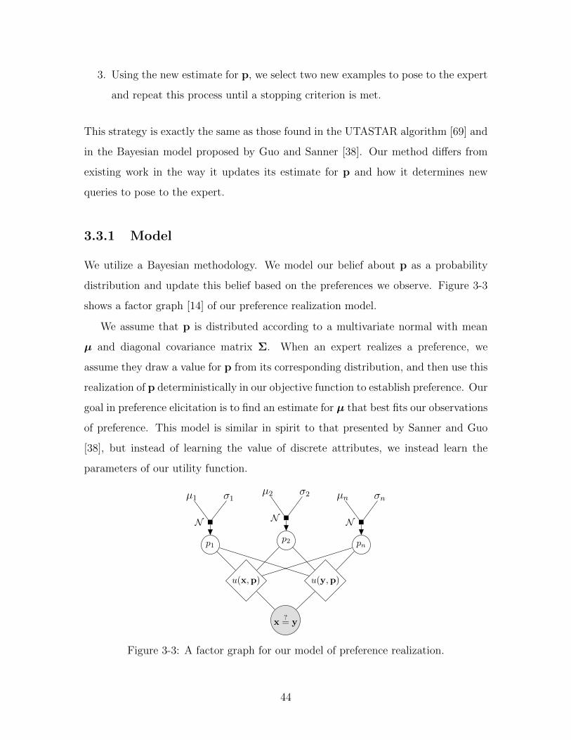
We utilize a Bayesian methodology. We model our belief about p as a probability

distribution and update this belief based on the preferences we observe. Figure 3-3

shows a factor graph [14] of our preference realization model.

We assume that p is distributed according to a multivariate normal with mean

µ and diagonal covariance matrix Σ. When an expert realizes a preference, we

assume they draw a value for p from its corresponding distribution, and then use this

realization of p deterministically in our objective function to establish preference. Our

goal in preference elicitation is to find an estimate for µ that best fits our observations

of preference. This model is similar in spirit to that presented by Sanner and Guo

[38], but instead of learning the value of discrete attributes, we instead learn the

parameters of our utility function.

x?= y

u(x,p) u(y,p)

p1p2 pn

µ1 σ1µ2 σ2 µn σn

N N N

Figure 3-3: A factor graph for our model of preference realization.

44

3.3.2 Inference

Inference on Figure 3-3 is difficult, as we can only observe p indirectly through re-

alizations of preference. Prior work uses expectation propagation [55] to exploit the

graphical nature of the problem and perform efficient inference [38, 39]. However,

this approach may not be desirable for engineering design optimization for several

reasons. First, existing implementations of expectation propagation on this graph

require the posterior of µ to be a multivariate normal with a diagonal covariance ma-

trix [38, 39]. Although this restriction can result in an approximate solution quickly,

in the context of engineering design optimization, we are willing to wait a few more

seconds for more accurate results. Furthermore, even if the posterior were to actually

be a diagonal covariance multivariate normal distribution, expectation propagation

would still only converge to an approximate solution for inference problems of this

structure [38, 39, 55].

Instead of expectation propagation, we will analytically derive our posterior up to

a normalizing constant. We let D denote our data—the set of preferences the expert

has given us. From Bayes’ Rule, we have that

P(µ,Σ | D) ∝ P(D | µ,Σ)P(µ,Σ) (3.6)

The P(µ,Σ) term is simply our prior, generally chosen to be a maximum entropy

distribution given our knowledge of the parameter. For example, we often have a

guess for the value of each element of µ and know its sign, so an exponential prior

on each element is a natural choice. The likelihood term differs from prior work in

an important way. Previous approaches add preferences one at a time. The prior is

updated using the preference as likelihood, and then the posterior is used as the prior

for the next preference [20, 38]. This cycle forces the authors to use approximation

algorithms, as the prior for the second preference is no longer Gaussian [38, 39]. Our

approach avoids this problem by viewing the set of preferences as our data. Thus,

as long as we are able to calculate our likelihood term, we can add a new preference

by incorporating it into our data and computing our posterior from scratch using our

45

original prior.

We can evaluate the likelihood term in two different ways. First, we present

an approach that exploits properties of linear functional forms of u(·) in order to

perform efficient inference. We then discuss a second approach which uses numerical

integration techniques to perform inference on nonlinear utility functions.

Linear Utility Functions

Suppose we have a linear utility function u(x) = pᵀx. We know that if x y, then

pᵀx > pᵀy⇒ pᵀ(x− y) > 0 (3.7)

In our model, p ∼ N (µ,Σ). To make the following steps easier to follow, we let

p , p− µ, which results in p ∼ N (0,Σ). Equation 3.7 then becomes

pᵀ(x− y) > −µᵀ(x− y) (3.8)

In order to calculate P(D | µ,Σ), we must find the probability that Equation 3.8 is

true. For example, if x− y = 〈1, 4〉, then this probability is the probability mass in

the shaded region of Figure 3-4.

x− y

p1

p2

Figure 3-4: Region for which Equation 3.8 is true.

In order to integrate over the shaded region in Figure 3-4, we exploit the fact that

the marginal distributions in any direction of multivariate normal distributions are

46

themselves univariate normal. The variance along the x− y direction is

σ2x−y = (x− y)ᵀΣ(x− y) (3.9)

and the distribution has a mean of zero. Consequently,

P (pᵀ(x− y) > −µᵀ(x− y)) = Φ

(µᵀ(x− y)

σ2x−y

)(3.10)

where Φ(·) is the normal cumulative distribution function. Equation 3.10 is thus the

probability that x y. Our model specifies that realizations of p are independently

drawn from their distributions. If we let D represent the subset of our preferences

that are strict, then

P(D | µ,Σ) =∏

(x,y)|xy

Φ

(µᵀ(x− y)

σ2x−y

)(3.11)

Equation 3.11 can be easily modified to account for indifference preferences. In-

stead of requiring that pᵀx > pᵀy, we simply require that pᵀx and pᵀy be within

some ε of each other. After some experimentation, setting ε = σ2x−y/2 has yielded

good results, which are shown in the empirical experiments later in this thesis. Using

this value for ε, the probability of our indifference preferences D∼ is

P(D∼ | µ,Σ) =∏

(x,y)|x∼y

(Φ

(µ · (x− y)

σ2x−y

+ 0.5

)− Φ

(µ · (x− y)

σ2x−y

− 0.5

))(3.12)

Because D⋃D∼ = D, we can combine Equations 3.11 and 3.12 to form our likeli-

hood function:

P(D | µ,Σ) = P(D | µ,Σ)P(D∼ | µ,Σ) (3.13)

We now know our posterior up to a normalizing constant, so we can use Markov

Chain Monte Carlo (MCMC) to sample directly from the posterior [54]. If p has low

dimensionality, the Metropolis algorithm will generally give the best samples. As the

dimensionality increases, Gibb’s sampling may be more effective. [35] The efficiency

47

of both methods is—as usual—dependent on the data. In our experience, we have

seen good performance with the Metropolis algorithm for up to a twelve-dimensional

p, as demonstrated later in our application section. Alternatively, if we only want a

point-estimate of µ, we can use an optimization algorithm to solve for the maximum

a-posteriori (MAP) estimate. If we let d = x− y, the µi partial derivatives of the

natural logarithm of Equation 3.6 are

∂ log(P(µ,Σ | D))∂µi

=∂ log(P(µ,Σ))

∂µi

+

∑(x,y)|xy

di

σ2x−y

φ(

µ·dσ2x−y

)Φ(

µ·dσ2x−y

)+

∑(x,y)|x∼y

di

σ2x−y

φ(

µ·dσ2x−y

+ 0.5)− φ

(µ·dσ2x−y− 0.5

)Φ(

µ·dσ2x−y

+ 0.5)− Φ

(µ·dσ2x−y− 0.5

)

(3.14)

where φ(·) designates the probability density function of the normal distribution. As

long as the log-priors on µ are partially-differentiable, then we can use Equation 3.14

in a gradient ascent method, such as BFGS [79], to solve for the MAP estimate to

arbitrary precision.

For computational purposes, it is often prudent to perform inference only on µ

by assuming Σ = σ2I, where I is the identity matrix and σ2 is a fixed constant. This

assumption can result in better convergence, and empirically we have found that the

model is not very sensitive to the choice of σ2. If σ2 is relatively small, the algorithm

converges somewhat faster if there are no inconsistent preferences, but somewhat

slower otherwise.

In fact, if we fix Σ as described above, then we can prove that the posterior is

log-concave for log-concave priors. Our proof begins with several lemmas.

Lemma 1. If D ∈ Rn×n is a diagonal matrix, and B ∈ Rn×n is a matrix consisting

of ones, then the product DBD is positive semidefinite.

Proof. If we let di | i ∈ 1 . . . n represent the elements on the diagonal of D, then

48

the product DBD is of the form

DBD =

d21 d1d2 · · · d1dn

d2d1 d22 · · · d2dn

......

. . ....

dnd1 dnd2 · · · d2n

(3.15)

By inspection, we see that vectors of the form vi = 〈−di, 0, . . . , 0, d1, 0, . . .〉, where the

d1 is the ith element, are linearly independent vectors, all with eigenvalues of zero.

There are n − 1 of these eigenvectors. The nth eigenvector is 〈d1, d2, . . . , dn〉, which

by inspection has a corresponding eigenvalue of∑

i d2i ≥ 0. Thus, because an n × n

matrix has exactly n eigenvalues, we have found them all, and all are non-negative.

Therefore, by definition DBD is positive semidefinite.

Lemma 2. The function Φ(x+ a)− Φ(x− a) is log-concave for all a ∈ R | a ≥ 0.

Proof. We know that φ(x) is log-concave[6]. Furthermore, we know that integrals

of log-concave functions are log-concave and products of log-concave functions are

themselves log-concave[59]. We let

g(z) =

1 if x− a ≤ z ≤ x+ a

0 otherwise

(3.16)

We know that g(z) is log-concave because it is an indicator function of a convex set.

Thus, φ(z)g(z) is log-concave and

∫Rφ(z)g(z)dz =

∫ x+a

x−a

φ(z)dz = Φ(x+ a)− Φ(x− a) (3.17)

is also log-concave.

49

If we let d = x− y, then the likelihood of our strict preferences is

P(D | µ,Σ) =∏

(x,y)|xy

Φ

(µᵀd

σ2d

)(3.18)

Lemma 3. The likelihood of our strict preferences is log-concave.

Proof. We take take the logarithm of Equation 3.18, yielding

log(P(D | µ,Σ)) =∑

(x,y)|xy

log

(Φ

(µᵀd

σ2d

))(3.19)

We let H(log(Φ)) be the Hessian matrix of one of the terms in the sum of Equation

3.19. We have that

H(log(Φ)) =f(µ)

σ2d

d21 d1d2 · · · d1dn

d2d1 d22 · · · d2dn

......

. . ....


(3.20)

where

f(µ) =−φ2(µ

ᵀdσ2d)

Φ2(µᵀdσ2d)

+−µφ(µᵀd

σ2d)

Φ(µᵀdσ2d)

(3.21)

We know that Equation 3.21 must be non-positive because it is of the same form as

the second derivative of the logarithm of Φ(x), which is known to be log-concave[6].

By Lemma 1, the matrix in equation 3.20 must be positive semidefinite. Because it

is being multiplied by a nonpositive scalar, H(log(Φ)) must be negative semidefinite.

Therefore, the Hessian of Equation 3.19 is a sum of negative semidefinite matrices,

which must also be negative semidefinite. Thus, the likelihood of our strict preferences

is log-concave.

Lemma 4. The likelihood of our indifference preferences is log-concave.

50

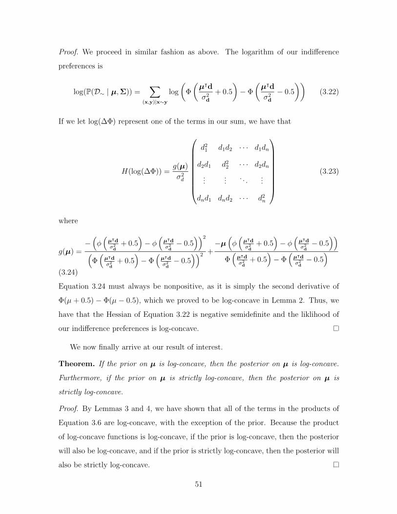
Proof. We proceed in similar fashion as above. The logarithm of our indifference

preferences is

log(P(D∼ | µ,Σ)) =∑

(x,y)|x∼y

log

(Φ

(µᵀd

σ2d

+ 0.5

)− Φ

(µᵀd

σ2d

− 0.5

))(3.22)

If we let log(∆Φ) represent one of the terms in our sum, we have that

H(log(∆Φ)) =g(µ)

σ2d

d21 d1d2 · · · d1dn

d2d1 d22 · · · d2dn

......

. . ....


(3.23)

where

g(µ) =−(φ(

µᵀdσ2d+ 0.5

)− φ

(µᵀdσ2d− 0.5

))2(Φ(

µᵀdσ2d+ 0.5

)− Φ

(µᵀdσ2d− 0.5

))2 +−µ

(φ(

µᵀdσ2d+ 0.5

)− φ

(µᵀdσ2d− 0.5

))Φ(

µᵀdσ2d+ 0.5

)− Φ

(µᵀdσ2d− 0.5

)(3.24)

Equation 3.24 must always be nonpositive, as it is simply the second derivative of

Φ(µ + 0.5) − Φ(µ − 0.5), which we proved to be log-concave in Lemma 2. Thus, we

have that the Hessian of Equation 3.22 is negative semidefinite and the liklihood of

our indifference preferences is log-concave.

We now finally arrive at our result of interest.

Theorem. If the prior on µ is log-concave, then the posterior on µ is log-concave.

Furthermore, if the prior on µ is strictly log-concave, then the posterior on µ is

strictly log-concave.

Proof. By Lemmas 3 and 4, we have shown that all of the terms in the products of

Equation 3.6 are log-concave, with the exception of the prior. Because the product

of log-concave functions is log-concave, if the prior is log-concave, then the posterior

will also be log-concave, and if the prior is strictly log-concave, then the posterior will

also be strictly log-concave.

51

This theorem is extremely useful, as most commonly-used priors—such as the ex-

ponential and normal distributions—are strictly log-concave. This results in several

important qualities for our posterior. First, if strict log-concavity holds, then there

exists exactly one local optimum, and that optimum is globally optimal [10]. Fur-

thermore, if strict log-concavity holds, BFGS will approach this global optimum in

superlinear time [58]. Finally, BFGS has been able to solve nonlinear optimization

problems with millions of variables [21], meaning we need not worry about our infer-

ence technique’s ability to scale to high dimensions. To our knowledge, this is the

first approach proven to converge quickly and accurately to the global MAP estimate

for any realistic number of dimensions.

Nonlinear Utility Functions

The likelihood function may not be able to be represented analytically for arbitrary

functional forms of the utility function. If we fix our covariance matrix to a constant

as described above, then our likelihood function is in general

P(D | µ,Σ) =∏

(x,y)∈D

∫Rn

I(x,y,p)n∏

i=1

φ

(pi − µi

σ

)dp (3.25)

where I(x,y,p) is in indicator function which is one whenever our utility function

ranks x and y in the same order as our expert’s preference and zero otherwise.

We can use an integral approximation technique to evaluate the right side of

Equation 3.25. For low dimensions, sparse grid quadrature rules can provide an

efficient estimate [36]. For higher dimensions, the most efficient numerical integration

technique is Monte-Carlo simulation.

With this approximation for for P(D | µ,Σ), we can either approximate the

MAP, or draw samples directly from the posterior. However, we must modify our

methodology to account for the fact that our likelihood function is now both noisy

and expensive to compute.

BFGS requires a large number of function evaluations and can struggle with noisy

functions, and consequently is no longer the preferred method for optimizing the likeli-

52

hood function to get the MAP. Instead, it is more efficient to use surrogate modelling

to find the MAP. Because our samples are now noisy, we must use regularization in

our surrogate model to avoid overfitting [33].

Alternatively, we can sample directly from the posterior using “pseudo-marginal”

MCMC. Although using noisy estimates for the likelihood function does result in

slower mixing, it still generates valid samples from the posterior [3]. In our expe-

rience, we achieved best mixing using the “Monte Carlo within Metropolis” variety

of pseudo-marginal MCMC [3]. Although this variant of pseudo-marginal MCMC is

the most costly per step, we have found that the superior mixing is worth the extra

computation.

Pseudo-marginal MCMC does pose significant computational challenges, but mod-

ern tools are starting to make this feasible. We implemented our algorithm in Julia

[13] and parallelized the inner integral approximation across four local cores. Using

1000 Monte Carlo samples to approximate P(D | µ,Σ)P(µ,Σ) and 1000 total pseudo-

marginal MCMC samples, we saw good convergence. On an Intel 3.5 GHz processor

running Linux, this process takes approximately 20 seconds for a three-dimensional

p and 20 preferences. For consumer-end preference elicitation, such as an internet

radio station automatically selecting the next song to play, this runtime would be

prohibitively long. However, for engineering design applications, this delay may be

tolerable if linear functional forms of u(·) are unacceptable.

3.3.3 Query Generation

Some preference queries are more useful than others. For example, suppose our utility

function is u(x1, x2) = p1x1 + p2x2 and we know p1 exactly, but have no information

about p2. Then, learning the expert’s preference between two designs with different

values for x1 and identical values for x2 yields no new information. In contrast,

knowledge about the user’s preference between two designs with identical values for

x1 and different values for x2 allows us to decrease our uncertainty about p2.

We utilize the concept of the entropy of a distribution [68] in order to analyze the

53

effectiveness of a query. The entropy of a distribution is defined as

H(X) , −∫

fX(x) log2 (fX(x)) dx (3.26)

where fX(x) is the probability density function of the random variable X.

Because we can sample from the posterior of the distribution, we can estimate its

entropy by fitting a kernel density approximation to the samples and calculating the

entropy of this approximation [46]. In order to determine the information encoded

by the query, we calculate the expected entropy for each possible comparison using

the following formula:

E(H(x

?= y

))≈ H(P(µ,Σ | D,x y)P(x y))+

H(P(µ,Σ | D,x ≺ y)P(x ≺ y)) + H(P(µ,Σ | D,x ∼ y)P(x ∼ y)) (3.27)

where H(·) denotes our entropy estimate via MCMC sampling and kernel density

estimation.

In order to determine the most effective query, we simply look at every possible

pairwise comparison between our family of candidate solutions and choose the one

with the lowest expected entropy, i.e., the query that most decreases our posterior

uncertainty. This entropy-minimization technique, pioneered in the 1950s [51], has

been used successfully in prior preference elicitation work [41, 52, 49] as well as other

machine learning work, such as pattern recognition [17].

If the number of possible comparisons is large, then this can be a computationally

intensive task, as each comparison requires three MCMC simulations. Fortunately, it

is trivially parallizable. Determining the best comparison for a linear utility function

among 100 possible comparisons with 10 pre-existing preferences takes approximately

10 seconds on a four core 3.5 GHz processor and scales linearly with the number of

possible comparisons.

Many existing preference elicitation algorithm use a related, but fundamentally

different, technique to generate queries. Instead of choosing the query that minimizes

54

posterior entropy, they choose the query that has the highest expected value of in-

formation [20, 41, 38]. This reduces the likelihood of the algorithm posing queries

between designs that are of no interest to the designer or designs that could not exist.

Maximizing expected value of information empirically results in the algorithm choos-

ing the best item from a set with the fewest number of queries [20, 38]. Unfortunately,

maximizing expected value is intractable for our engineering design optimization ap-

plication. We wish to maximize over the set of all possible designs, rather than maxi-

mizing utility over a set of already known designs—in order to calculate the expected

value of information, we would have to be able to evaluate every possible design. If

we could do this, we would have no need of optimization in the first place. However,

if we use the the entropy minimization technique in the optimize-elicit-optimize loop,

we know will not encounter infeasible designs: all the designs available for comparison

have already been generated by the previous stage of optimization. Finally, although

entropy-maximization may pose queries between designs that are intrinsically of no

interest to the designer, the designer’s preference between these designs may help the

optimization make similar value choices between better performing designs.

3.4 Results

In order to test the performance of this algorithm, we first contrive a simple example

to examine the algorithm’s convergence properties. Then, we apply the algorithm to

optimizing an aircraft collision avoidance system.

3.4.1 Proof of Concept

We first test the ability of our algorithm to converge to a known utility function. We

let u(x) = pᵀx and arbitrarily set p = 〈5,−1, 2〉. We generated 100 designs randomly,

with each of the three metrics being drawn randomly from a uniform distribution over

the interval [0, 1]. Our goal is to measure how effectively our algorithm can estimate

p by receiving only pairwise preferences between the designs.

One way to measure preference elicitation algorithm performance is to calculate

55

the difference in utility between the estimated optimal solution and the true optimal

solution [20]. Although this definition is useful in applications where the set of possible

solutions is already known, in an optimization context we do not know the global

optimal solution, and simply assigning utility to existing solutions does not help

us generate new ones. Instead, we are far more concerned with matching the actual

underlying utility function globally, as it will be the force that drives our optimization

routine.

To measure how close we are to the global utility function, we compare our es-

timate for the parameter vector p to the known p. One might be tempted to use

a norm of p − p to measure our accuracy. However, for linear utility functions, it

is impossible to learn p to anything beyond a normalizing constant by only using

pairwise comparisons, as if pᵀx > pᵀy, then cpᵀx > cpᵀy for all c ∈ R+. Thus, we

use the angle between our estimate p and p as our loss function V :

V (p,p) = arccos

(pᵀp

‖p‖2‖p‖2

)(3.28)

In fact, this notion of error angle will correlate highly with the loss in utility of

the global optimum. If our utility function is linear, then we know that the global

optimum will occur on the boundary of the design set [12]. Thus, the error in angle

will correspond to how far away the estimated optimum is from the true optimum on

the boundary. For example, if the set of all designs forms a unit hypersphere around

the origin and the true p is normalized, then the loss in utility from an error angle

of θ is simply 1− cos(θ). This correspondence is shown in Figure 3-5.

We test our method using randomly-generated queries and queries generated using

the entropy minimization technique. Our method was compared against a modifica-

tion of the UTASTAR [69] algorithm.1 We also test a heuristic for query generation

common in the literature of selecting the current best solution and the one with the

highest probability of improving upon the incumbent [38]. These four methods are

1As described in the source, the UTASTAR algorithm fits a piecewise linear approximation tothe utility function. However, such approximations do not extrapolate well globally, so we added aconstraint that forces the estimated utility function to be exactly linear.

56

Metric 1

Metric 2

True Optimum

L

Estimated Optimum

θ

Figure 3-5: Correspondence between loss in utility L and error angle θ for a circulardesign set.

shown in Table 3.1.

Many existing preference elicitation methods are not tested because they are not

applicable to our task of learning parameters of the utility function itself. Most

existing methods simply try to find the optimal item from a given set without trying

to find the functional form of the utility function directly [38, 41, 77, 20]. Furthermore,

we know that methods based on the expected value of information [20, 38, 77] are not

useful, as the utility over all possible designs is dependent on the exact structure of

the set of all possible designs—although we might be able to perform this integration

for a toy problem where we prescribe this set, it is extremely doubtful we would ever

be able to calculate it for a real engineering design optimization problem.

All tests begin with the same first query, which was randomly generated. For the

Bayesian tests, a flat prior was used. Each test was repeated 100 times.

With an Infallible Expert

We first run the above algorithms using an infallible expert—in our test, a subroutine

that calculates the true utility of both of the query objects, and returns the true

preference between the two. Figure 3-6 shows the mean loss for each method as a

function of the number of preferences given to the algorithm.

The entropy-based learning method performs best, followed by the Bayesian ran-

57

Table 3.1: Description of the four algorithms tested.

Method Description

UTASTAR with RandomThe UTASTAR Algorithm with randomly chosenqueries to the expert. UTASTAR has no methodfor posing queries to the expert.

Bayesian with RandomOur Bayesian approach, learning from querieschosen at random.

Bayesian with Best/Highest PI

Our Bayesian approach, learning from queriesgenerated using the heuristic of querying the esti-mated best against the solution with the highestprobability of improvement.

Bayesian with Min EntropyOur Bayesian approach, learning from queriesthat most decrease expected posterior entropy.

0

10

20

30

40

10 20 30 40 50Preferences Given

MeanLoss

Strategy

UTASTAR, with Random

Bayesian, with Random

Bayesian, with Best/Highest PI

Bayesian, with Min Entropy

Figure 3-6: Mean loss as a function of preferences given from an infallible expert.

dom and linear programming methodologies. Performing significantly worse than

the others is the best/highest probability of improvement heuristic. Although this

heuristic fares well when a more traditional loss function is used [38], it performs

poorly at learning the true underlying function. This is because this heuristic con-

strains the queries to always include the current optimum, even when a query between

lower-ranked alternatives would have been more informative to global understanding.

58

Table 3.2 shows the statistical tests performed on the algorithm performance.

We used the bootstrap [30] to generate 104 new samples from our performance data

and calculated how often the mean performance of each algorithm did not match the

ordering in Figure 3-6. This provides a result similar to a Student’s t-test, but without

requiring that our data be normally distributed. [30, 62] These results indicate that

the trends exhibited in Figure 3-6 are statistically significant.

Table 3.2: Pairwise statistical comparison tests for best performing algorithms withan infallible expert.

Event P(Event)

Entropy ≥ UTASTAR 0.0000

Entropy ≥ Random 0.0140

Random ≥ UTASTAR 0.0046

With a Fallible Expert

We know that in reality no expert is infallible. Instead of a subfunction that ob-

serves the true utility to make comparisons, we incorporate the blunder model from

Bradley and Terry [16], modified to account for indifference preferences in the manner

described by Guo and Sanner [38]. Given true objective values u(x) and u(y), the

probability of returning an indifference preference is

P(x ∼ y | u(x), u(y)) = exp (−β|u(x)− u(y)|) (3.29)

Given that an indifference preference is not returned, the probability of returning a

strict preference is

P(x y | u(x), u(y),¬(x ∼ y)) =exp (α(u(x)− u(y)))

1 + exp (α(u(x)− u(y)))(3.30)

The parameters α and β allow this model to represent experts who have varying

degrees of confusion. For this test, we let α = 1 and β = 0.1, which led to a reasonable

number of indifference and inconsistent preferences in our contrived scenario.

59

0

25

50

75

100

10 20 30 40 50Preferences Given

MeanLoss

Strategy

UTASTAR, with Random

Bayesian, with Random

Bayesian, with Best/Highest PI

Bayesian, with Min Entropy

Figure 3-7: Mean loss as a function of preferences given from a fallible expert.

After programming this model of fallibility into our test, we again ran 100 sam-

ples of our four methodologies. Figure 3-7 shows the decay of error means as more

preferences are added, and Table 3.3 shows the bootstrap statistical tests comparing

the difference between the best performing algorithms.

Table 3.3: Pairwise statistical comparison tests for best performing algorithms witha fallible expert.

Event P(Event)

Entropy ≥ Best/Highest PI 0.0000

Entropy ≥ Random 0.0000

Random ≥ Best/Highest PI 0.0000

Clearly, our Bayesian methodology is far more robust to noise than the linear

programming formulation, which only performs marginally better than randomly

guessing weight vectors. Even the ”Best with Highest Probability of Improvement”

heuristic, when used with our framework, performs dramatically better. Furthermore,

the entropy-based query selection method continues to outperform selecting random

queries and the best/highest expected improvement heuristic.

It is also interesting to note that UTASTAR generally seems to be unable to

60

converge beyond a certain point. This highlights one of the fundamental problems in

robust linear optimization: the linear program has likely determined that the actual

solution lies within some polyhedral set, but is forced to always pick an extreme point

of the polyhedron [12]. If the most likely solution is in the interior, linear programming

will never be able to select it. When there are no contradictory preferences, the

polyhedron of possible solutions grows smaller with the addition of the cutting plane

defined by each preference, allowing the algorithm to converge. The presence of

contradictory preferences prevents the polyhedron from reducing its volume beyond

a certain point, as inconsistent preferences will re-expand it.

We have shown that our Bayesian approach performs very well. It converges

quickly and accurately to the true utility function, even in the presence of noisy

preferences. Encouraged by these results, we then used our approach to optimize

ACAS-X.

3.4.2 Application to Aircraft Collision Avoidance

Background

Optimizing the POMDP penalties in ACAS-X is incredibly difficult. The mapping

between the penalties and system performance is known to be non-convex [71] —

although many real-world non-convex optimization problems can be optimized satis-

factorily by using heuristics such as simulated annealing [76], genetic algorithms [70],

or particle swarm optimization [57], all these methods presume that the objective

function is computationally easy to evaluate [76, 70, 57]. Evaluating our POMDP

solution is not so: at 25 minutes per evaluation, a genetic algorithm with a meager

population size of 100 would take over nearly three months to produce 50 generations

of solutions. The slow evaluation time also precludes the use of multi-objective op-

timiztion procedures based on these heuristic methods, such as the NSGA-II [26] or

ant-colony optimization [23, 22]. We therefore use the surrogate modelling optimiza-

tion method [71].

This technique requires a single objective, but we are concerned with several

61

objectives, such as the safety of the system and the number of nuisance alerts. We

could use goal programming to define a single metric, but it is unclear what the

ideal point should be, and even less clear what the distance metric should be. The

ε-constraint method is just as troublesome, as we often do not know what constraints

would be appropriate at the onset of optimization, and even if we did, the mapping

between the POMDP penalties and the system performance is too complex for us

to even be able to define the constraints. Consequently, we resort to the simplest

solution: defining a utility function. For each of these metrics, we define the marginal

utility function to be

umetric = exp

((metric)2

(metric target)2

)(3.31)

and we let the overall utility be

u =∑

i∈metrics

piui (3.32)

where pi indicates the relative importance of achieving the target rate for that metric.

We casually refer to these pi as the metric’s “weight.” By adjusting these weights,

the behavior of our surrogate modelling optimization can drastically change. To learn

these weights, we will use our preference elicitation algorithm.

Small-Scale Testing

In order to test the effect of our preference elicitation on our optimization routine,

we perform a simple test. We vary only two of the most important parameters in

our POMDP formulation and measure only the safety and nuisance alert metrics.

Initial weights were chosen naıvely and are shown in Table 3.4. After 50 surrogate

modeling iterations, we branch our optimization as shown in Figure 3-8. One branch

continues with the naıve weights, while the other uses new weights derived from

expert preference elicitation on the first 50 samples. The prior distribution used on

each weight was an exponential distribution with a mean of the naıve weight.

As a basis for the preferences, the expert choose policies that struck a suitable

balance between operational suitability and safety. Table 3.4 compares the weights

62

Base 50 Samples

50 Samples withNew Weights

50 Samples withOld Weights

Figure 3-8: Our Small-Scale Optimization Test.

4e-05

5e-05

6e-05

7e-05

8e-05

Without With

Sim

ulatedNM

AC

Rate

Solution Safety

0.30

0.35

0.40

0.45

0.50

Without With

Sim

ulatedNuisance

Alerts

Solution Operational Suitability

Figure 3-9: Distribution of solutions found with and without preference elicitation.The base 50 samples are omitted.

used before and after preference elicitation.

Table 3.4: Weights before and after preference elicitation.

Metric Original Weight Inferred Weight

NMAC Rate 0.990 0.508

RA Rate 0.010 0.492

Figure 3-9 shows the distribution of solutions returned by the optimization in a

box-and-whisker plot with and without the use of preference elicitation. Without the

preference elicitation, the optimization routine searches far too heavily in the safety

63

domain without sufficient regard to the operational suitability. With the aid of several

pairwise comparisons, the optimization routine returns results far more tailored to

the expert’s goals.

Application

Surrogate modelling optimization of the aircraft collision avoidance system POMDP

took several months. The eight most important penalties in the POMDP were tuned

using the surrogate modelling framework, and twelve safety and operational suitability

metrics were measured for each design. Due to the potentially sensitive nature of

the trade-offs involved in designing an aircraft collision avoidance system, we have

included the metric values but omitted the names of the metrics. In doing so, we

hope to demonstrate the usefulness of our preference elicitation algorithm without

putting our sponsor’s priorities on public trial.

We began our optimization by setting each of the pi in Equation 3.32 by intuition

for each of our twelve metrics. These values are shown in the “Weights, Before”

column of Table 3.5. We then ran the surrogate modelling optimization for several

weeks with these pi, generated and evaluating a large number of ACAS-X policies. The

average performance of these policies is shown in the “Mean Metric Values, Before”

column of Table 3.5. We took five of the top performing policies and presented them

to the international aviation safety community, consisting of the Federal Aviation

Administration (FAA), the Single European Sky Air traffic management Research

(SESAR) project, potential commercial vendors, and pilot associations. We asked

them to provide preferences between these designs based on their stake in the project

in addition to heuristic feedback about the quality of the designs. The heuristic

feedback amounted to the following:

Performance in metrics 1 and 2 are performing above expectations.

Metrics 3 and 4 should be improved. If need be, this may be at the expense of

metrics 1 and 2.

Metric 12 needs improvement.

64

Table 3.5: Effect of preference elicitation on collision avoidance optimization.

Weights Mean Metric Values

Before After Before After

Metric 1 0.0750 0.0540 2.567 · 10−5 2.566 · 10−5

Metric 2 0.2250 0.0932 2.227 · 10−6 2.228 · 10−6

Metric 3 0.1225 0.1472 0.4977 0.4657

Metric 4 0.0350 0.0589 0.4643 0.4274

Metric 5 0.1050 0.0771 0.1097 0.1265

Metric 6 0.0175 0.1190 0.0033 0.0034

Metric 7 0.0350 0.0385 0.0097 0.0129

Metric 8 0.0350 0.0448 0.0426 0.0295

Metric 9 0.1700 0.0371 0.1356 0.1479

Metric 10 0.0300 0.0470 0.6461 0.6298

Metric 11 0.1000 0.0500 0.1264 0.0123

Metric 12 0.0500 0.2320 0.0147 0.0143

Instead of using the heuristic feedback to manually adjust the weights, we simply

took the preferences elicited from the international community and fed them into our

preference elicitation algorithm. Priors on each mean were selected to be exponential

with a mean of the previously used, intuition-based value for each pi. We fixed the σ

of our algorithm to be 0.1. After running our algorithm, we used the posterior mean of

each µi as a point estimate for each pi. These estimates are shown in in the “Weights,

After” column of Table 3.5. As we can see, the new weight structure matched the

heuristic feedback provided by the international community. The weights on metrics

1 and 2 decreased relative to metrics 3 and 4, and the weight on metric 12 increased.

The “Mean Metric Values, After” column of Table 3.5 shows the metric perfor-

mance using the new weights derived from preference elicitation. As we hoped, the

performance in metrics 3, 4, and 12 improved. Interestingly, the performance in met-

rics 1 and 2 did not degrade substantially after the weight change. Feedback from the

program sponsors of the top designs returned from the second stage of optimization

were very positive — they were satisfied with the balance of metrics these designs

exhibited.

65

As promising as this may be, we note that one should be cautious in interpreting

Table 3.5, as the metrics values before and after preference elicitation are not inde-

pendent. Because the optimization after preference elicitation started from where

the optimization before preference elicitation ended, we would naturally expect the

metric values to improve. In order to perform a fully rigorous test, we would have to

re-run the optimization without the preference elicitation and compare the two op-

timizations. Unfortunately, because of the large amount of resources and manpower

necessary for these optimizations, we were unable to perform this experiment. That

said, we do not think it is too much of a leap of faith to believe that an optimization

with different metric weights will return different results.

We have since used the optimize-elicit-optimize loop above several times to in-

corporate preferences into our optimization. Each time, our preference elicitation

algorithm performed as above: it satisfied as many preferences as possible, didn’t

stray too far from our prior estimates, and matched the heuristic commentary pro-

vided alongside the preferences. Although we recognize that the plural of “anecdote”

is not “data,” we believe that our successful applications of our algorithm demonstrate

its usefulness to real-world engineering design optimization problems.

3.5 Discussion

We have shown that our method for preference elicitation is well-suited for use in engi-

neering design optimization. Its inference method is less restrictive and more general

than existing work, and its ability to use entropy-minimization to generate queries

results in it converging faster to the true utility function than other preference elicita-

tion algorithms. We then successfully used our framework to incorporate preferences

from dozens of experts around the world into a multiple month-long optimization

routine of ACAS-X.

66

Chapter 4

Multi-Objective Optimization

Most large-scale optimizations of engineering designs rely on the use of utility func-

tions in some form, whether this utility function is specified manually, learned through

some preference elicitation algorithm, or defined via some goal programming metric.

Although this does not pose any issues if the utility function is defined perfectly, in

reality we know that this will not be the case.

In this chapter, we review methods one can use for a multiobjective optimization

problem without specifying a utility function. Although these methods are often

limiting, we identify an aspect of ACAS-X conducive to these methods. In Section 4.2,

we use a multiobjective genetic algorithm to identify shortcomings of the ACAS-X

TA system, and then use the same genetic algorithm to tune a new TA policy to

optimal performance.

4.1 Background

Figure 4-1 illustrates what occurs with a faulty utility function. Suppose the dots lie

on the actual Pareto front, and the arrow indicates the direction of search specified

by our (linear) utility function. We can visualize how the points on the Pareto front

would be ranked by our utility function by projecting them onto the arrow.

As we can see, if our actual optimum is near the head of the arrow, the optimum

will be ranked highly and likely be found during optimization of our utility function.

67

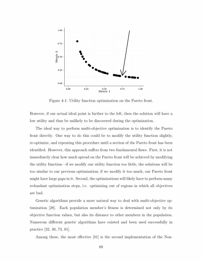
0.00

0.25

0.50

0.75

1.00

0.00 0.25 0.50 0.75 1.00Metric 1

Metric

2

Figure 4-1: Utility function optimization on the Pareto front.

However, if our actual ideal point is further to the left, then the solution will have a

low utility and thus be unlikely to be discovered during the optimization.

The ideal way to perform multi-objective optimization is to identify the Pareto

front directly. One way to do this could be to modify the utility function slightly,

re-optimize, and repeating this procedure until a section of the Pareto front has been

identified. However, this approach suffers from two fundamental flaws. First, it is not

immediately clear how much spread on the Pareto front will be achieved by modifying

the utility function—if we modify our utility function too little, the solutions will be

too similar to our previous optimization; if we modify it too much, our Pareto front

might have large gaps in it. Second, the optimizations will likely have to perform many

redundant optimization steps, i.e. optimizing out of regions in which all objectives

are bad.

Genetic algorithms provide a more natural way to deal with multi-objective op-

timization [28]. Each population member’s fitness is determined not only by its

objective function values, but also its distance to other members in the population.

Numerous different genetic algorithms have existed and been used successfully in

practice [32, 40, 73, 81].

Among these, the most effective [81] is the second implementation of the Non-

68

dominated Sorting Genetic Algorithm (NSGA-II) [26]. The fitness function of the

NSGA-II is straightforward. First, each individual is assigned a “Dominance Count.”

Individuals on the current Pareto front of the population are assigned a domination

count of 0. These individuals are then removed, and the Pareto front is again recal-

culated. Members on this new Pareto front are given a domination count of 1, and

this procedure continues until enough individuals are identified to form the parents

of the next generation. If the last dominance front provides too many individuals for

the population size, then the individuals whose absence makes the largest gap in the

Pareto front are chosen [26]. A single generation of the NSGA-II runs inO(mn2) time,

where m is the number of objectives, and n is the number of population members

[26].

Although theO(mn2) computational overhead of the NSGA-II is rarely a problem,

its large number of calls to the function to be optimized can be problematic if the

function is computationally expensive. If we run 100 generations of a population size

of 100, then the function must be called a total of 5000 times—if we were to apply

this to ACAS-X as a whole, this would take over four months.

This chapter applies the NSGA-II algorithm to the ACAS-X project. A funda-

mental insight into how TAs are generated allows for our function of interest to be

optimized directly using the NSGA-II algorithm.

4.2 Traffic Alert Optimization

Traffic Alerts (TAs) warn a pilot of nearby aircraft that could potentially become a

threat, ensuring the pilot is alert and prepared for an RA to be issued. TCAS simply

extends its RA heuristics to greater values of τ to determine if an TA should be issued

[1]. However, this results in the TCAS TA logic falling prey to the same issues as

the RA logic: the system is inherently unrobust, and therefore must be made very

sensitive to ensure acceptable safety.

Puntin and Kochenderfer [60] previously developed a method for issuing TAs that

appeared to be successful for ACAS-X. However, as the ACAS-X project evolved,

69

their method proved no longer viable. In this section, we review their approach and

discuss its empirical shortcomings. Aided by the NSGA-II [26], we then modify their

strategy, resulting in across-the-board improvement of the ACAS-X TA logic.

4.2.1 Traffic Alert Mechanism

After the implementation of ACAS-X RA logic as an POMDP, simply extending the

τ value was no longer a sensible option [60]. One approach would be to develop

another POMDP model specifically for TA logic. However, Puntin and Kochenderfer

describe some of the problems with such an approach:

In order to do this optimization, it is necessary to define a probabilistic

dynamic model and a cost function that defines the objective of the sys-

tem. The dynamic model would capture the response of the pilots to the

generation of the RA. Although the function of the TA is not to instruct

the pilots to maneuver, pilots often do, and so this should be accounted

for in the model. The model can also capture the fact that a TA often im-

proves the swiftness of the pilot response to an RA. The resulting TA cost

can be a function of whether an NMAC occurs and the disruptiveness of

the alerts. In order to implement such an optimization, the current model

used for optimizing the RAs would have to be expanded to account for

the additional TA state data, resulting in larger lookup tables [60].

This approach could be feasible, but would require extensive study and analysis.

Furthermore, the increase in the state space would dramatically increase the size of

the cost table, making it potentially too big to run on available aircraft hardware.

Puntin and Kochenderfer instead propose an alternate procedure: when the system

looks up the per action cost for RAs, it uses these costs to determine if an TA should

be issued. Specifically, the logic follows Algorithm 1 to determine if an TA should be

issued or turned off [60]. This algorithm works by using the clear-of-conflict reward

as a proxy for safety. Generally, the lower the reward for issuing clear-of-conflict, the

70

1 // TA On Logic2 if COC COST < COC ON AND3 COC COST − minCOSTS \ COC COST < COST DIFFERENTIAL

4 then5 TA ← ON;6 end7 // TA-Off Logic8 if COC COST > COC OFF AND9 TIME SINCE RA ≥ 6 seconds AND

10 TA DURATION ≥ 6 seconds11 then12 TA ← OFF13 end

Algorithm 1: ACAS-X TA logic.

less safe the aircraft is. The same logic is used in Line 8 to determine when a TA

should be turned off, after the minimum TA time has been achieved.

However, the clear-of-conflict cost alone was determined to be insufficient for de-

termining if a TA should be turned on. The logic encoded in Line 2 requires that not

only the clear-of-conflict reward to be sufficiently low, but also that the reward of the

next-best action is within some threshold of the clear-of-conflict reward. Puntin and

Kochenderfer explain the logic behind this:

The [COST DIFFERENTIAL] threshold was added to reduce the rate of nui-

sance TAs. Without the [COST DIFFERENTIAL] threshold, there were many

TAs caused by the COC cost crossing the on threshold when all other

actions had much higher costs. Implementing a [COST DIFFERENTIAL]

threshold requirement suppressed the TAs when an RA was not likely

due to the large separation between the cost of COC and the other ac-

tions [60].

By looking only at the action costs already calculated for the RA logic, this

approach results in no increase in offline optimization, no increased table storage

requirements, and very little online computation. However, this algorithm requires

specification of the COC ON (Line 2), COC OFF (Line 8), and COST DIFFERENTIAL (Line

71

3) parameters. Optimal values for these parameters are far from clear, and can only

be learned though optimization.

4.2.2 Optimization

Like the rest of ACAS-X, TA logic performance can only be measured through ex-

tensive simulation. For assessing TA performance, three metrics are deemed most

important [60]:

Number of Traffic Alerts.

Number of surprise RAs. A surprise RA is an RA that did not have an TA at

least six seconds prior.

Number of segmented TAs. A segmented TA is a TA that goes off, but then

back on again later in the encounter. This behavior is perceived to undermine

pilot confidence in the system.

Average TA duration. A TA that runs too long after the threat has been resolved

could also undermine pilot confidence in the system.

In mathematical terminology, we thus have a function f : R3 → R4 that we wish to

optimize.

Puntin et. al. optimized these parameters by discretizing the parameter space and

evaluating the solutions at all discretized points [60]. Although trivial to implement,

this approach took enormous computing resources, taking over a week on a high

performance compute cluster. Furthermore, if the discretization is too coarse, then

good solutions could be missed.

We could optimize TA logic through our surrogate modelling optimization pro-

cedure. However, this procedure is slow and requires specification of an objective

function — we have already shown this to be problematic. Instead, we exploit the

fact that the metrics of interest in TA optimization are largely independent of pilot’s

response to TAs. This observation was confirmed by flight safety experts at the FAA.

72

By instructing our simulated pilots to ignore TAs and only respond to RAs, we

can drastically speed up evaluation of TAs logic on simulations. The positions, belief

states, RA costs and actions will always be the same, regardless of what values we

assign to the TA parameters. Thus, if we collect the RA cost values at every point

in time for every simulation, we can effectively simulate different TA logic by simply

performing Algorithm 1 on the archived RA costs. Instead of actually simulating

aircraft dynamics for hundreds of thousands of aircraft encounters, we need only

parse a file.

A natural concern for this methodology is the memory requirement. At each time

step, we need to collect the following values to run Algorithm 1:

A time index of the simulation (8 bit integer).

The clear-of-conflict cost (64 bit floating point).

The difference between the clear-of-conflict cost and the next best alternative

(64 bit floating point).

Whether an RA was issued at this timestep (8 bit boolean).

This results in 144 bits of data per simulation timestep. The average simulation

duration is approximately 100 seconds, and observations are recorded at one Hertz.

Consequently, we can fit information from one million simulations into memory on a

high performance computer: it only takes up 13.4 GB.

This methodology dramatically decreases logic evaluation performance. The time

to evaluate a single aircraft collision encounter is cut from 0.25 seconds to 1.66 ·

10−5 seconds. Including overhead costs, simulating our TA encounter set of 100,000

encounters directly takes approximately three minutes on a 64 node high performance

compute cluster; our parsing evaluation strategy evaluates the same encounter set

locally in serial in 1.67 seconds.

This dramatic decrease in runtime allows us to directly optimize the TA logic

without creating a series of surrogate models. Because we are dealing with a multi-

73

objective optimization problem of relatively low dimension, the NSGA-II is a natural

choice.

We can further exploit the conditional independence inherent in our problem. The

number of TAs and surprise TAs is dependent only on specification of the COC ON and

COST DIFFERENTIAL parameters. Furthermore, given a set of values for the COC ON

and COST DIFFERENTIAL parameters, the number of segmented TAs and the average

TA time can be tuned by only modifying the COC OFF parameter. Thus, instead of

optimizing a function f : R3 → R4, we can optimize f : R2 → R2 and then simply

tune a function g : R→ R2. This independence drastically reduces the dimensionality

of the optimization problem, reducing our runtime by orders of magnitude.

4.2.3 Results

Initial Results

After collecting the cost data for 100,000 simulations based on real-world traffic en-

counters, we ran the NSGA-II to optimize our traffic alert performance. We used a

parent population size of 100, the simulated binary crossover [2] breeding technique,

and ran the algorithm for 50 generations. Run in serial, this optimization takes

approximately 40 minutes.

Figure 4-2 shows the results of this optimization alongside TCAS performance on

the same dataset. This result is concerning for ACAS-X. In order to issue the same

number of TAs, ACAS-X would have to risk tripling the number of surprise RAs; to

keep the number of surprise RAs the same, the number of TAs would have to double.

The result is not a relic of the NSGA-II. In an effort to validate these results, a

week-long brute force space search was performed. This search yielded results of a

similar nature to Figure 4-2, indicating that the optimization method was performing

as expected, and that the underlying issue lie in the POMDP TA logic.

This conflicts with the results presented by Puntin et al [60]. Since their publica-

tion, ACAS-X RA logic has undergone significant changes designed to increase safety

in certain encounters with high vertical rates as well as to reduce the number of alters

74

0

10

20

30

40

50

1000 2000 3000 4000Traffic Alerts

Surp

rise

RA’s

System

ACAS

TCAS

Figure 4-2: Traffic alert Pareto front.

in certain planned level-off scenarios. These changes fundamentally altered the cost

behavior in many scenarios, resulting in different TA performance.

Traffic Alert Logic Change

The results of our NSGA-II optimization indicated that Algorithm 1 is not sufficient

to outperform TCAS for our POMDP policy. In order to investigate the source of this

performance problem, we created a plot of our POMDP policy. If aircraft velocities

are constant, then the alert issued by ACAS-X is uniquely determined by the relative

altitudes of the aircraft and the time until the aircraft’s Closest Point of Approach

(CPA). Figure 4-3 shows the ACAS-X policy for two level aircraft flying directly at

each other at a speed of 250 knots. For example, if the intruder aircraft is 20 seconds

from closest point of approach and is 200 feet above the ACAS-X-equipped aircraft,

the ACAS-X aircraft will receive command to “climb at 1500 feet per minute.” The

fraction associated with each RA refers to the acceleration in G’s at which pilots are

75

instructed to respond to this alert.

−10−505101520253035404550

−1,400

−1,200

−1,000

−800

−600

−400

−200

0

200

400

600

800

1,000

1,200

1,400

Seconds to CPA

RelativeAltitude(ft)

No Data

CoC

DNC2000 14

DND2000 14

DNC1000 14

DND1000 14

DNC500 14

DND500 14

DNC 14

DND 14

MTN 14

DSC1500 14

CL1500 14

DSC1500 13

CL1500 13

DSC2500 13

CL2500 13

MTLO

TA

Figure 4-3: Traffic Alert policy plot for original logic.

Figure 4-3 reveals the failure modes of Figure 1. First, there exist several “teeth”

in the policy at the edges of the alerting region (approximately at ± 600 ft, 20

seconds until CPA). These edges lead to unnecessary TAs: if the system was in

clear-of-conflict when the aircraft were closer in altitude, then there is no reason

why the aircraft should be in a traffic alert at this altitude difference. These edges

are likely a result of the altitude discretization used in the POMDP interacting in a

complex way with Algorithm 1.

The other failure mode in Figure 4-3 is the large gap at the center of the policy

(at 0 altitude difference, 25 seconds to CPA). In the RA logic, such a gap can be

explained due to the uncertainty in the POMDP: if the system is unsure of which

aircraft has a higher altitude, than it is safer to wait a few seconds to decide which

76

aircraft should climb rather than running the risk of giving the wrong aircraft the

climb order and driving the aircraft into one another. However, for TA logic, such a

delay is senseless: the system will alert in a few seconds regardless of what happens;

the system is only delaying to decide which alert is optimal. Thus, in the gap, the

clear of conflict reward is very low, but all the alternatives are simply worse.

This observation gives insight on how to improve Algorithm 1: the AND condition

at Line 2 is causing the policy to delay issuing a TA in the gap, as the clear-of-conflict

reward is low, but no alternative is sufficiently close. A better policy might be to use

and OR condition at Line 2: this would allow the COST DIFFERENTIAL condition to

activate most TAs, but allow the COC ON condition to activate TAs in the gaps in

Figure 4-3.

After implementing the OR variety of Algorithm 1, we created a policy plot for

our new TA algorithm. This is shown in Figure 4-4.

Figure 4-4 shows that both fundamental problems with the policy depicted in

Figure 4-3 are resolved. As expected, using the OR condition resulted in the gap

being filled, reducing the number or surprise RAs in our policy. An unexpected

benefit was the removal of the “teeth” from Figure 4-3. Thus, based on this policy

plot, we would expect that the OR policy should in result both fewer alerts and fewer

surprise RAs than the AND policy in Algorithm 1.

Post-Change Results

We then ran the NSGA-II optimization algorithm on the new OR-based policy. The

results from this optimization are shown in Figure 4-5.

As we had hoped, switching the AND to OR significantly shifted the policy, re-

sulting in far fewer TAs for every surprise RA. In fact, there are points on the OR

Pareto curve that completely dominate TCAS performance, achieving both fewer TAs

and surprise RAs.

The Pareto front from Figure 4-4 was given to FAA experts, who analyzed and

selected the policy most suited to their use cases. After selecting the values for COC ON

and COST DIFFERENTIAL, we simply manually tuned the COC OFF threshold until the

77

−10−505101520253035404550

−1,400

−1,200

−1,000

−800

−600

−400

−200

0

200

400

600

800

1,000

1,200

1,400

Seconds to Closest Point of Approach

RelativeAltitude(ft)

No Data

CoC

DNC2000 14

DND2000 14

DNC1000 14

DND1000 14

DNC500 14

DND500 14

DNC 14

DND 14

MTN 14

DSC1500 14

CL1500 14

DSC1500 13

CL1500 13

DSC2500 13

CL2500 13

MTLO

TA

Figure 4-4: Traffic Alert policy plot for modified OR logic.

number of segmented TAs was reduced to an acceptable level. In fact, the optimal

level for COC OFF resulted in the OR-based policy having fewer segmented TAs and a

lower average TA duration. Table 4.1 shows how our final policy compares to TCAS

in the four metrics of interest.

Table 4.1: Comparison of TCAS and ACAS traffic alert performance.

TAs Surprise RAs Segmented TAs Mean TA Duration

TCAS 1224 13 31 24.33

ACAS-X 1056 13 11 22.86

% Reduction 13.7% 0% 64.5% 6.1%

Table 4.1 shows across-the-board improvement in the ACAS-X TA logic with

respect to our objective metrics. However, not all performance can be captured in

78

0

10

20

30

40

50

1000 2000 3000 4000Traffic Alerts

Surp

rise

RA’s System

ACAS with AND

ACAS with OR

TCAS

Figure 4-5: Pareto Front after Logic Change.

a single objective metric. One such abstract measure of performance is the shape of

the distribution of the TA leadtime: the amount of time before an RA was issued

that a TA was active. For example, if a TA was issued at seven seconds and an RA

was issued at seventeen seconds, then this encounter would have a ten second TA

leadtime. This is a generalization of the “surprise RA” metric.

Figure 4-6 shows the distribution of TA leadtimes for both the TCAS and ACAS-X

systems. The general shape of the distribution is similar; in both systems, most RAs

have a ten to twenty second leadtime, which is considered optimal by FAA experts.

Furthermore, we also note that our ACAS-X methodology results in fewer TAs with

a very long leadtime. This is also promising: long TAs can also be dangerous, as the

pilot may have forgotten about the TA by the time the RA is issued.

79

0

5

10

15

20

0 10 20 30 40 50Lead Time (s)

Occurence

sSystem

ACAS

TCAS

Figure 4-6: Distribution of time difference between TA and RA after logic change.The vertical bar at six seconds is the threshold for a surprise RA.

4.3 Discussion

Although not practical in all applications, identifying the Pareto front directly can

be very useful in engineering design optimization. In the case of ACAS-X TA logic,

its use demonstrated that a fundamental change in the TA logic was necessary. By

examining the POMDP policy, we were able to identify and implement that change.

This change resulted in a shift in the Pareto front, providing us a number of designs

that dominated TCAS performance. The final point selected for use outperformed

TCAS dramatically in all relevant performance metrics.

80

Chapter 5

Conclusion

5.1 Summary

In this thesis, we have implemented two approaches to deal with multi-objective

optimization in the realm of aircraft collision avoidance. First, we developed a novel

algorithm for preference elicitation to allow the designers to more accurately create

utility functions. Then, we applied a multi-objective genetic algorithm to optimize

the behavior of traffic alerts in the ACAS system.

To develop our preference elicitation algorithm, we began by examining existing

literature, and determined that although useful in some consumer-end applications,

none existed that were amiable to eliciting a utility function for engineering design

optimization. By exploiting properties of an existing model, we developed a faster,

more accurate, and less-restrictive inference technique. We also developed a new ap-

proach to posing queries to the expert based on posterior entropy maximization. We

then empirically showed that our method converged faster to a user’s true preference

model than existing algorithms. This result also held when we used a more com-

plex response model. Finally, we applied this algorithm to the surrogate modeling

optimization of ACAS-X.

When optimizing traffic performance in ACAS-X, we showed that we can quickly

evaluate encounters when we only modify traffic alert logic parameters. This speedup

enabled us to use the NSGA-II genetic algorithm to identify the Pareto front of our

81

solution space. The use of this algorithm allowed us to identify a fundamental flaw

in the TA logic, which we corrected. Re-running the genetic algorithm then resulted

in across-the-board improvement of the traffic alert behavior in the ACAS-X system.

5.2 Further Work

Within our preference elicitation algorithm, further work will be done on query selec-

tion. Sampling from the posterior of every possible preference realization is computa-

tionally expensive. It may be possible to find a heuristic to quickly determine which

queries have a chance of being informative, and simply use the posterior sampling

method to break the tie between these top queries.

It may also be possible to exploit the fact that our inference method does not

require our covariance matrix to be diagonal—in other words, we could introduce

correlation between the realizations of the elements of our parameter vector. Intu-

itively, it might make sense for there to be a small, negative correlation between the

elements: if the expert overestimates the value of one metric, he or she is likely un-

derestimating the value of others. Adding this negative correlation could make our

method converge more quickly to a real expert’s true utility function.

Work on the TA system also remains. First, the new system will be analyzed

encounter-by-encounter by FAA experts to ensure that said TA are reasonable from

a pilot acceptability standpoint — there may be cases in which pilots actually want

an TA, which would have been missed by our TA minimization paradigm.

A larger concern lies in that the TA logic is build exclusively off the RA logic.

Because the RA state space only extends 40 seconds prior to CPA, it is currently

impossible for a TA to be issued before then. Thus, if a TA is issued at 35 seconds

prior to CPA, then it will always result in a surprise RA. This problem cannot be

mitigated without expanding the state space. However, extending the state space to

include time steps up to 60 seconds would result in a 50% increase in both runtime

for solving the POMDP as well as memory required for the optimal policy. The

memory problem can be mitigated at the expense of code complexity by storing only

82

the clear of conflict cost and the next best option cost for time steps greater than

40, resulting in an increased memory requirement of only 6.25%. However, in either

case, the increase in memory size could require the system to be implemented on a

different hardware, potentially dramatically increasing program costs. A study will

be undertaken to evaluate the benefit of expanding the state space beyond 40 seconds

as well as if the system would require a hardware upgrade.

It may also be possible to generalize TA logic using techniques from machine

learning. First, we would run a simulation and collect the costs for each action at

each time step. Then, based on the simulation results, we can determine which time

steps should have had a TA present; a reasonable approach would be to mark the

six seconds prior to any RA as time steps that should have a TA. By doing this

for a large number of simulations, we create a set of labeled data. We can thus use

machine learning on this data to create a model that predicts whether or not a TA

should be present based on the cost values. ACAS-X could then use this model in

real time to determine when it should give a TA. Preliminary efforts have shown this

to be a feasible methodology; unfortunately, these results are too experimental for

this publication.

83


84

Bibliography

[1] Federal Aviation Administration. Introduction to TCAS-II, February 2011.

[2] Ram Bhusan Agrawal, Kalyanmoy Deb, Kalyanmoy Deb, and Ram BhushanAgrawal. Simulated binary crossover for continuous search space. Technicalreport, 1994.

[3] Christophe Andrieu and Gareth Roberts. The pseudo-marginal approach forefficient Monte Carlo computations. The Annals of Statistics, 37(2):697–725,2009.

[4] Dana Angluin. Queries and concept learning. Machine Learning, 2(4):319–342,1988.

[5] Dylan Asmar. Airborne collision avoidance in mixed equipage environments.Master’s thesis, Massachusetts Instituite of Technology, 77 Massachusetts Ave,Cambridge, MA, 2013.

[6] Mark Bagnoli and Ted Bergstrom. Log-concave probability and its applications.Economic Theory, 26(2):445–469, 2005.

[7] Ashok D. Belegundu and Tirupathi R. Chandrupatla. Optimization Conceptsand Applications in Engineering. Cambridge University Press, second edition,2011.

[8] Alain Berlinet and Christine Thomas-Agnan. Reproducing kernel Hilbert spacesin probability and statistics, volume 3. Springer, 2004.

[9] Dimitri P Bertsekas. Dynamic programming and optimal control, volume 1.Athena Scientific Belmont, MA, 1995.

[10] Dimitri P Bertsekas. Nonlinear programming. Athena Scientific, 1999.

[11] Dimitri P. Bertsekas and John N. Tsitsiklis. Introduction to Probability. AthenaScientific, 2002.

[12] Dimitris Bertsimas and John N Tsitsiklis. Introduction to Linear Optimization,volume 6. Athena Scientific Belmont, MA, 1997.

[13] Jeff Bezanson, Stefan Karpinski, Viral B. Shah, and Alan Edelman. Julia: Afast dynamic language for technical computing, 2012. arXiv cs-PL/1209.5145.

85

[14] Christopher M. Bishop. Pattern Recognition and Machine Learning. Springer,2006.

[15] Craig Boutilier. A POMDP formulation of preference elicitation problems.In AAAI Innovative Applications of Artificial Intelligence Conference, pages239–246, 2002.

[16] Ralph Allan Bradley and Milton E Terry. Rank analysis of incomplete blockdesigns: I. the method of paired comparisons. Biometrika, 39(3-4):324–345,1952.

[17] Matthew Brand. Pattern discovery via entropy minimization. Technical ReportTR-98-21, MERL– A Mitshubishi Electric Research Laboratory, 1998.

[18] Darius Braziunas. Computational approaches to preference elicitation. Depart-ment of Computer Science, University of Toronto, Tech. Rep, 2006.

[19] Sebastian Burhenne, Dirk Jacob, and Gregor P Henze. Sampling based on sobolsequences for monte carlo techniques applied to building simulations. Proceedingsof Building Simulation, 2011.

[20] Urszula Chajewska, Daphne Koller, and Ronald Parr. Making rational decisionsusing adaptive utility elicitation. In AAAI Innovative Applications of ArtificialIntelligence Conference, pages 363–369, 2000.

[21] Weizhu Chen, Zhenghao Wang, and Jingren Zhou. Large-scale l-bfgs usingmapreduce. In Advances in Neural Information Processing Systems, pages1332–1340, 2014.

[22] Manuel Chica, Oscar Cordon, Sergio Damas, and Joaqun Bautista. Includingdifferent kinds of preferences in a multi-objective ant algorithm for time andspace assembly line balancing on different nissan scenarios. Expert Systems withApplications, 38(1):709 – 720, 2011.

[23] Manuel Chica, Oscar Cordon, Sergio Damas, and Joaqun Bautista. Interactivepreferences in multiobjective ant colony optimisation for assembly line balancing.Soft Computing, pages 1–13, 2014.

[24] Vincent Conitzer. Eliciting single-peaked preferences using comparison queries.Journal of Artificial Intelligence Research, 35:161–191, 2009.

[25] Thomas Dean, Leslie Pack Kaelbling, Jak Kirman, and Ann Nicholson. Planningunder time constraints in stochastic domains. Artificial Intelligence, 76(12):35 –74, 1995. Planning and Scheduling.

[26] K. Deb, A Pratap, S. Agarwal, and T. Meyarivan. A fast and elitist multiobjec-tive genetic algorithm: Nsga-ii. IEEE Transactions on Evolutionary Computa-tion, 6(2):182–197, Apr 2002.

86

[27] Kalyanmoy Deb. Multi-objective optimization. In Search Methodologies, pages403–449. Springer, 2014.

[28] Kalyanmoy Deb and Deb Kalyanmoy. Multi-Objective Optimization Using Evo-lutionary Algorithms. John Wiley & Sons, Inc., New York, NY, USA, 2001.

[29] James S Dyer. Mautmultiattribute utility theory. In Multiple criteria decisionanalysis: state of the art surveys, pages 265–292. Springer, 2005.

[30] B. Efron. Bootstrap methods: Another look at the jackknife. The Annals ofStatistics, 7(1):pp. 1–26, 1979.

[31] Theodoros Evgeniou, Massimiliano Pontil, and Tomaso Poggio. Regularizationnetworks and support vector machines. Advances in Computational Mathematics,13(1):1–50, 2000.

[32] Carlos M Fonseca, Peter J Fleming, et al. Genetic algorithms for multiobjectiveoptimization: Formulation, discussion and generalization. In ICGA, volume 93,pages 416–423, 1993.

[33] Alexander I.J. Forrester, Andras Sobester, and Andy J. Keane. Engineering De-sign via Surrogate Modelling: A Practical Guide. American Instituite of Aero-nautics and Astronautics, 2008.

[34] Xavier Gandibleux. Multiple Criteria Optimization: State of the Art AnnotatedBibliographic Surveys, volume 52. Springer Science & Business Media, 2002.

[35] Stuart Geman and Donald Geman. Stochastic relaxation, gibbs distributions,and the bayesian restoration of images. In IEEE Transactions on Pattern Anal-ysis and Machine Intelligence, number 6, pages 721–741. IEEE, 1984.

[36] Thomas Gerstner and Michael Griebel. Numerical integration using sparse grids.Numerical Algorithms, 18(3-4):209–232, 1998.

[37] Yoav Goldberg and Michael Elhadad. splitsvm: Fast, space-efficient, non-heuristic, polynomial kernel computation for nlp applications. In Proceedingsof the 46th Annual Meeting of the Association for Computational Linguistics onHuman Language Technologies: Short Papers, HLT-Short ’08, pages 237–240,Stroudsburg, PA, USA, 2008. Association for Computational Linguistics.

[38] Shengbo Guo and Scott Sanner. Real-time multiattribute Bayesian preferenceelicitation with pairwise comparison queries. In International Conference onArtificial Intelligence and Statistics, pages 289–296, 2010.

[39] Ralf Herbrich, Tom Minka, and Thore Graepel. Trueskill: A bayesian skill ratingsystem. In Advances in Neural Information Processing Systems, pages 569–576,2006.

87

[40] Jeffrey Horn, Nicholas Nafpliotis, and David E Goldberg. A niched pareto geneticalgorithm for multiobjective optimization. In Evolutionary Computation, 1994.IEEE World Congress on Computational Intelligence, pages 82–87. Institute ofElectrical and Electronics Engineers, 1994.

[41] Neil Houlsby, Ferenc Huszar, Zoubin Ghahramani, and Jose M.Hernandez-lobato. Collaborative gaussian processes for preference learn-ing. In F. Pereira, C.J.C. Burges, L. Bottou, and K.Q. Weinberger, editors,Advances in Neural Information Processing Systems 25, pages 2096–2104.Curran Associates, Inc., 2012.

[42] Ralph L Keeney and Howard Raiffa. Decisions with multiple objectives: prefer-ences and value trade-offs. Cambridge university press, 1993.

[43] A. Khvilivitzky. Visual collision avoidance system for unmanned aerial vehicles,December 3 1996. US Patent 5,581,250.

[44] Mykel J. Kochenderfer, Jessica Holland, and James Chryssanthacopoulos. Next-generation airborne collision avoidance system. Lincoln Laboratory Journal,19(1):17–33, 2012.

[45] JSH Kornbluth. A survey of goal programming. Omega, 1(2):193–205, 1973.

[46] A Kramer, J. Hasenauer, F. Allgower, and N. Radde. Computation of the pos-terior entropy in a bayesian framework for parameter estimation in biologicalnetworks. In IEEE Conference on Control Applications, pages 493–498, 2010.

[47] James K. Kuchar. Methodology for alerting-system performance evaluation.Journal of Guidance, Control, and Dynamics, 19(2):438–444, 1996.

[48] Taku Kudo and Yuji Matsumoto. Fast methods for kernel-based text analysis.In Proceedings of the 41st Annual Meeting on Association for ComputationalLinguistics-Volume 1, pages 24–31. Association for Computational Linguistics,2003.

[49] Neil Lawrence, Matthias Seeger, and Ralf Herbrich. Fast Sparse Gaussian ProcessMethods: The Informative Vector Machine. In Proceedings of the 16th AnnualConference on Neural Information Processing Systems, pages 609–616, 2003.

[50] Yann LeCun, Sumit Chopra, Raia Hadsell, M Ranzato, and F Huang. A tutorialon energy-based learning. Predicting Structured Data, 2006.

[51] D.V. Lindley. On a measure of the information provided by an experiment. TheAnnals of Mathematical Statistics, 27(4).

[52] D MacKay. Information-based objective functions for active data selection. Neu-ral Computation, 4(4):590–604, July 1992.

88

[53] R.T. Marler and J.S. Arora. Survey of multi-objective optimization methods forengineering. Structural and Multidisciplinary Optimization, 26(6):369–395, 2004.

[54] Nicholas Metropolis, Arianna W. Rosenbluth, Marshall N. Rosenbluth, Au-gusta H. Teller, and Edward Teller. Equation of state calculations by fast com-puting machines. The Journal of Chemical Physics, 21(6):1087–1092, 1953.

[55] Thomas P. Minka. Expectation propagation for approximate bayesian inference.In Conference on Uncertainty in Artificial Intelligence, pages 362–369, 2001.

[56] Quirino Paris. The dual of the least-squares method. Technical report, March2012.

[57] Riccardo Poli, James Kennedy, and Tim Blackwell. Particle swarm optimization.Swarm intelligence, 1(1):33–57, 2007.

[58] Michael J.D. Powell. Some global convergence properties of a variable metricalgorithm for minimization without exact line searches. Nonlinear programming,9:53–72, 1976.

[59] Andras Prekopa. On logarithmic concave measures and functions. Acta Scien-tiarum Mathematicarum, 34:335–343, 1973.

[60] Brendon Puntin and Mykel J. Kochenderfer. Traffic alert optimization for air-borne collision avoidance systems. Encounters, 1(786,088):2–300, 2013.

[61] Rita Almeida Ribeiro. Fuzzy multiple attribute decision making: A review andnew preference elicitation techniques. Fuzzy Sets and Systems, 78(2):155 – 181,1996. Fuzzy Multiple Criteria Decision Making.

[62] John Rice. Mathematical statistics and data analysis. Cengage Learning, 2006.

[63] Ryan Rifkin, Gene Yeo, and Tomaso Poggio. Regularized least-squares classi-fication. Nato Science Series Sub Series III Computer and Systems Sciences,190:131–154, 2003.

[64] Lorenzo Rosasco and Tomaso Poggio. A Regularization Tour of Machine Learn-ing: MIT-9.520 Lecture Notes, December 2014. Manuscript.

[65] Stuart Russelll and Peter Norvig. Artificial Intelligence: A Modern Approach.Prentice Hall, Upper Saddle River, New Jersey, 3 edition, 2009.

[66] Jerome Sacks, William J Welch, Toby J Mitchell, and Henry P Wynn. Designand analysis of computer experiments. Statistical science, pages 409–423, 1989.

[67] Bernhard Scholkopf, Ralf Herbrich, and Alex J Smola. A generalized representertheorem. In Computational learning theory, pages 416–426. Springer, 2001.

[68] C. E. Shannon. A mathematical theory of communication. The Bell SystemTechnical Journal, 27:379–423,623–656, 1948.

89

[69] Yannis Siskos. Encyclopedia of Optimization, volume 1. Springer, 2008.

[70] SN Sivanandam and SN Deepa. Genetic Algorithm Optimization Problems.Springer, 2008.

[71] Kyle Smith. Collision avoidance system optimization for closely spaced paralleloperations through surrogate modeling. Master’s thesis, Massachusetts Instituiteof Technology, 77 Massachusetts Ave, Cambridge, MA, 2013.

[72] Kyle Smith, Mykel J. Kochenderfer, Wesley Olson, and Adan Vela. Collisionavoidance system optimization for closely spaced parallel operations throughsurrogate modeling. In AIAA Guidance, Navigation, and Control Conference,2013.

[73] Nidamarthi Srinivas and Kalyanmoy Deb. Muiltiobjective optimization us-ing nondominated sorting in genetic algorithms. Evolutionary computation,2(3):221–248, 1994.

[74] Michael Stein. Large sample properties of simulations using latin hypercubesampling. Technometrics, 29(2):143–151, 1987.

[75] Andrea Tacchetti, Pavan K. Mallapragada, Matteo Santoro, and LorenzoRosasco. GURLS: A least squares library for supervised learning. Journal ofMachine Learning Research, 14:3201–3205, 2013. Source Code.

[76] Peter J.M. van Laarhoven and Emile H.L. Aarts. Simulated annealing. In Sim-ulated Annealing: Theory and Applications, volume 37 of Mathematics and ItsApplications, pages 7–15. Springer Netherlands, 1987.

[77] Paolo Viappiani and Craig Boutilier. Optimal bayesian recommendation setsand myopically optimal choice query sets. In J.D. Lafferty, C.K.I. Williams,J. Shawe-Taylor, R.S. Zemel, and A. Culotta, editors, Advances in Neural Infor-mation Processing Systems 23, pages 2352–2360. Curran Associates, Inc., 2010.

[78] John Von Neumann and Oskar Morgenstern. Theory of Games and EconomicBehavior. Princeton university press, 60th anniversary commemorative edition,2007.

[79] Ya-xiang Yuan. A modified BFGS algorithm for unconstrained optimization.IMA Journal of Numerical Analysis, 11(3):325–332, 1991.

[80] Ali MS Zalzala and Peter J Fleming. Genetic Algorithms in Engineering Systems,volume 55. Institution of Engineering and Technology, 1997.

[81] Eckart Zitzler and Lothar Thiele. Multiobjective optimization using evolutionaryalgorithms. In Parallel Problem Solving from Nature, volume 1498 of LectureNotes in Computer Science, pages 292–301. Springer Berlin Heidelberg, 1998.

90

Multi-Objective Optimization of Next-Generation Aircraft ...

Documents

Transcript of Multi-Objective Optimization of Next-Generation Aircraft ...