Multi-Fidelity Trajectory Optimization with Response...

American Institute of Aeronautics and Astronautics

092407

1

Multi-Fidelity Trajectory Optimization with Response Surface-Based Aerodynamic Prediction

Colonno, M. R.1 Stanford University, Palo Alto, California, Zip 94305 and Space Exploration Technologies, Hawthorne, CA, 90250

Reddy, S.2

Space Exploration Technologies, Hawthorne, California, 90250

and

Alonso, J. J .3 Stanford University, Palo Alto, California, Zip 94305

A methodology for the optimization of general atmospheric trajectories is presented. The trajectory optimization problem is formulated as a constrained minimization problem then discretized for use with a Gauss pseudospectral method. Assuming a robust optimizer, the fidelity of an optimum solution is limited by the accurate prediction of input physics. These include aerodynamic properties, atmospheric properties, wind velocity and direction, and mass properties. In addition, the free stream conditions at which aerodynamic simulations are performed are, in turn, a function of the trajectory and vary with mission. Here, a Kriging surface method is proposed which allows for the efficient adaptive sampling of subsequent physical data for increased levels of fidelity. This adaptive approach to high-fidelity physical data decreases the cost and cycle time required for mission planning or day-of-launch criteria. Results from an ascent and reentry example are presented and discussed in the context of current methods.

Nomenclature a = semimajor axis CD = drag coefficient CL = lift coefficient d = unit vector in drag direction e = eccentricity EIF = expected improvement function f = generic function F = thrust g = gravitational acceleration vector g0 = gravitational acceleration at planet’s surface h = altitude i = inclination Isp = specific impulse J = optimization objective function l = length scale l = unit vector in lift direction M = Mach number m = mass 1 Chief Aerodynamic Engineer, Space Exploration Technologies, Member AIAA 2 Dynamics Engineer, Space Exploration Technologies, Member AIAA 3 Associate Professor, Aeronautics & Astronautics, Stanford University, Member AIAA

46th AIAA Aerospace Sciences Meeting and Exhibit7 - 10 January 2008, Reno, Nevada

AIAA 2008-218

Copyright © 2008 by the American Institute of Aeronautics and Astronautics, Inc. All rights reserved.


092407

2

p = pressure p = vector of orbital parameters q = dynamic pressure (ρ∞V∞

2/2) R = planetary radius Re = Reynolds number Re’ = Reynolds number per unit length r = unit vector in the radial (vertical) direction S = reference area for aerodynamic coefficients s = interpolation error T = temperature [T] = coordinate transformation matrix t = time tb = burn time u = thrust direction unit vector V = velocity W = control stability constraint x = axial direction x = position vector y = vector in response surface variable space α = angle of attack β = yaw angle γ = ratio of specific heats w = rotation rate vector μ = planetary gravitational constant = Gmplanet ρ = density Ω = longitude of the ascending node ω = argument of periapsis ν = true anomaly Subscripts 0 = initial state CP = center of pressure G = gimbal location (thrust vector control) f = final state ∞ = ambient (free stream) E = Earth ECI = Earth-centered inertial coordinates o = orbital value P = propellant PL = payload Superscripts T = transpose • = rate (∂/∂t) ‘ = predicted by response surface

I. Introduction HE high cost of access to space places great emphasis on the efficient design of launch vehicles and the subsequent optimization of trajectories for maximum performance. With a fixed launch vehicle design, ascent

trajectories are optimized for a given payload and desired set of orbital parameters. This optimization process necessarily depends on a robust method for dynamic optimization and a multidisciplinary set of physical input data. The latter generally includes aerodynamic properties of the vehicle over a wide Mach range, detailed mass property

T


092407

3

data which is constantly changing as propellant mass is expelled, and atmospheric data (including wind conditions) which may be taken just before launch or reentry. All of these sources of data have associated uncertainties which must be accounted for in establishing the mission margin and day-of-launch liftoff criteria. Since margin must be established to cover all reasonable uncertainties, increased uncertainty results in smaller mass delivered to orbit. Algorithms to solve general dynamic optimization (or applied optimal control) problems have evolved over time from the original work of Byrson1,2 to many more recent solution methods3,4,5,7,14. Here, we use a Gauss pseudospectral method (GPM) of Ref. 3 through the TOMLAB GPOCS software19. GPOCS is an example of a direct solution method in which the continuous-time optimal control problem is transcribed into a nonlinear programming problem (NLP) which is subsequently solved using any well-established algorithms (SNOPT6 in the case of GPOCS). This is contrasted with an indirect solution method in which the first-order necessary conditions for optimality are analytically derived from the optimal control problem itself and the subsequent boundary-value problem solved numerically for extremal paths. Current numerical methods for trajectory optimization are discussed in greater detail in Refs. 4,5,14 among others. With a robust dynamic optimization tool, the fidelity-limiting aspect of trajectory optimization shifts to the physical input data. In this paper we are primarily concerned with: 1) the quantification and minimization of uncertainties in physical data through adaptive sampling, 2) maximizing flight performance over a range of mission profiles, and 3) providing a rapid-response means by which to establish liftoff criteria with manageable computational cost. Items (1) and (2) are addressed during mission planning while (3) is dependent upon atmospheric conditions evaluated before launch. The goal of this work is to provide a means by which a trajectory can be optimized to a specified level of uncertainty with minimal computational cost or (in many cases equivalently) the minimum cycle time.

II. Problem Formulation: Ascent Dynamic optimization or applied optimal control problems are generally formulated as constrained

minimizations in which the equations of motion are treated as constraint functions. A vector of continuous control parameters are sought which extremize a function of the state variables, often at the end of the time period of interest. This general problem statement is then discretized for use with an appropriate numerical method to perform the actual optimization. The sections below detail the objective and constraint functions for a general three degree of freedom (3-DOF) launch vehicle ascent problem.

A. Equations of Motion Here, we begin with the 3-DOF equations of motion in Earth-center-inertial (ECI) coordinates (named by

convention, this formulation is general to any central gravitational field) for a general multi-stage vehicle, Eqs. (1). When properly scaled, Eqs. (1) form a non-stiff set of ten coupled ordinary differential equations (ODEs). These were chosen for convenience and numerical performance, but any reference frame can be used.

( )( )

wu

xglduV

Vx

=∂∂

−=∂∂

+++=∂

∂

=∂

∂

∞∞

t

mtm

SqCSqCFmt

t

i

LDiECI

ECIECI

&

1

(1)

The vector u is the thrust direction which, in the 3-DOF approximation, we assume is also the vehicle orientation. Here, we use the rate of change of u, or w, as the control parameter making u a “pseudostate”. This formulation allows constraints to easily be placed on w continuously or at the endpoints of each stage’s flight. The thrust and mass flow vary for each stage, denoted by the subscript i. For a multi-stage vehicle, discontinuities occur in the vehicle mass between stages as the previous stage’s empty structural mass is released which require a multi-phase formulation of the optimal control problem. These are accounted for numerically with link conditions on each of the state variables, Eqs. (2). The lift and drag forces act parallel to and perpendicular to the total relative air velocity (Vtot), respectively. These directions are denoted by the unit vectors d and l in Eqs. (1). The gravitational


092407

4

acceleration, g(x), can be as detailed as required, but the spherical approximation (g directed along –r) and J2 oblateness correction of the WGS8417 model are commonly used.

0

0

0

ji

ji

jiECI

jiECI

=Δ

−=Δ

=Δ

=Δ

→

→

→

→

u

V

x

iSmm (2)

To complete the problem formulation the objective, boundary conditions (constraints which are evaluated at the initial and final times of each stage), and path constraints (constraints which are evaluated continuously in time) must be defined. These are discussed in the sections below. We seek the vector u(t) which minimizes J subject to the equations of motion (EOM) and the constraints discussed below.

B. Objective For ascent trajectories, the objective is simple: minimize the propellant mass required to deliver the payload mass, mPL, to the desired orbit. This is equivalent to maximizing the mass at the end of flight (burnout mass), stated as a minimization problem in Eq. (3). Note that the final time tf is, therefore, not known a priori. For trajectories which do not include a coast phase this is equivalent to a minimum time problem. It is not know a prior if m(tf) is positive; the mission may not be possible and the optimization procedure must account for cases in which the vehicle has insufficient performance.

)( ftmJ −= (3)

C. Boundary Conditions The initial conditions xECI(t0) and VECI(t0) are set by the location of the launch site, with initial velocity equal to the local rotational speed of the planet (if any). m(t0) is simply the gross liftoff mass. The initial orientation vector is assumed to be vertical, u(t0) = r. The boundary conditions at tf are more complex, requiring insertion into an orbit with the desired set of orbital elements p = {a,i,e,Ω,ω}T, summarized below. These are transformed into ECI coordinates (and vice versa) at tf to establish xECI(tf) and VECI(tf), while m(tf) is unconstrained as the target of the optimization. Note that the orbital elements listed above lack the true anomaly, ν, as we assume the insertion can take place anywhere on the desired orbit. Hence, the boundary conditions xECI(tf) and VECI(tf) are not unique. During a stage separation event a brief coast phase is typically required to fully shutdown the previous stage’s propulsion system, engage the separation system, and activate the current stage’s propulsion system. Depending on the stage sizing and desired orbit, burnout may occur at altitudes where aerodynamic forces are still significant. Without any thrust to counter aerodynamic moments, the new stage can rotate off course or collide with the previous stage during separation. Hence, limits on α at burnout may be placed on each stage. No constraints are placed on u(tf), though w = 0 may be desirable at tf and at stage burnouts.

D. Path Constraints Any number of additional constraints can be placed on the flight depending on the vehicle used, the requirements of the payload, and the mission. These constraints may be placed directly on the state or control variables or on functions thereof. Typical constraints include maximum axial and lateral accelerations, maximum q∞α product, maximum stagnation point heat transfer, and rotation rates during flight and at stage burnouts. The normalization of the orientation vector u is also treated as a path constraint. Refer to the launch vehicle example below for some specific constraint examples. A simplified stability criterion is also included to account for limitations on the vehicle’s control system. When neglecting the rotational DOFs, no limits on the moments about the vehicle center of gravity (CG). When the transient behavior of the control system and the vehicle structural dynamics are included, the rate of change of the moment is often the stability-limiting criterion. For ascent trajectories, this is primarily a function of the wind shear or rate of change of the aerodynamic moment. A single instantaneous criterion is insufficient because stability is a function of both the wind shear’s duration and amplitude. Changes in wind velocity which have high amplitude but


092407

5

short apparent duration (product of the vehicle’s vertical speed and rate of change with altitude) or low amplitude and long duration are generally not a stability concern. Here, we use the stability criterion Wij(t,τj), Eq. (4), an integration over a pulse duration τ which must be defined through an independent control system analysis. The integrated lift force rate is normalized with respect to the maximum side force which can be exerted by the control system. No specification is made about the type of control system, which may involve trust vector control (TVC), aerodynamic surfaces, or both. The length scales lCP and lG are representative of the moment arm between the center of pressure (CP) and the CG and the point at which control forces are applied (for most launch vehicle profiles, the total vehicle or stage length is applicable) and the CG, respectively. In general, the CP location itself is a function of M∞ and α but is presently assumed to be constant over the relatively short duration τ. The integration duration may be a function of flight time to account for changes in the vehicle mass properties. Alternatively, several different values of τ could be used to form several different constraints. (The subscript ij refers to the ith stage and jth pulse duration.) It is worth noting that the |∂CL/∂t| term is a function of both the vehicles aerodynamic properties and wind conditions. Application of the stability constraint Wij assumes a passively unstable vehicle with CP forward of the CG. For passively stable vehicles or stages this constraint is neglected.

),()()sin(

2/

2/maxjij

t

t

L

G

CP

i

i tWdtt

Ctqll

FS

i

τδ

τ

τ

≤∂∂

⎟⎟⎠

⎞⎜⎜⎝

⎛∫

+

−

∞ (4)

III. Physical Data Evaluation of Eqs. (1) requires a set of multidisciplinary physical data, including aerodynamic properties, wind

data and a gravitational model. We will assume that gravitational acceleration as a function of position, g(x), is known a priori. In addition, we will assume that the vehicle liftoff and burnout masses are measured with associated uncertainties. (It is noted that a 6-DOF simulations would additionally require the moment of inertia matrix as a function of vehicle mass.) Aerodynamic data and atmospheric conditions, including the wind velocity, are required. The sections below detail the data required in each category and the limitations on currently available tools.

A. Aerodynamic Properties The aerodynamic properties of the launch vehicle are typically the most expensive to determine and cannot, in

general, be refined adaptively close to the time of launch. For a 3-DOF simulation the vehicle is treated as a point mass having a lift and drag coefficients which are functions, in general, of M∞, α, and Re. For vehicles which are not axisymmetric, the sideslip angle β would additionally be required and some assumption would have to be made about the vehicle’s roll orientation during flight. Here, the Reynolds number per unit length, Re’, is used for convenience since it is a function of the free stream coefficients only (equivalent to taking the length scale in Re = 1.0 m). In a 6-DOF analysis, the aerodynamic side (yawing) force and moments or CP location would be required to evaluate the rotational degrees of freedom. Summarizing, the 3-DOF optimization requires CL(M∞,α, Re’) and CD(M∞,α, Re’) data throughout the flight. One of the greatest challenges of launch vehicle aerodynamics is the large range of flow conditions over which data is required. This includes values of M∞ from zero to 25 or greater, widely varying flow physics, and possibly large values of α early in flight due to wind. Fortunately from a trajectory optimization standpoint, the density (and hence dynamic pressure) typically falls to very small values before the physics of the free stream gases changes from a continuum fluid. However, the trajectory is not known a priori and a continuous, differentiable evaluation of the aerodynamic forces is required for an optimization algorithm such as that of GPOCS. Whether aerodynamic data comes from wind tunnel testing or computational fluid dynamics (CFD), it is unlikely to span the required range of flow conditions. Typically, data is available in the subsonic and lower supersonic M∞ range while data at very high M∞ has to extrapolated. Care must be taken to examine the M∞ → 0 and M∞ → ∞ limits for all aerodynamic coefficients to avoid infinite or negative values. Though q∞ → 0 at these limits, numerical instabilities or inaccurate solutions may result. Refer to the example in the following section for a specific discussion. Ascent trajectories with typical launch vehicle properties tend to result in maximum q∞ conditions in the low supersonic range while reentry trajectories tend to experience maximum q∞ conditions at much high M∞, placing additional emphasis on high-fidelity aerodynamic data in the hypersonic range.


092407

6

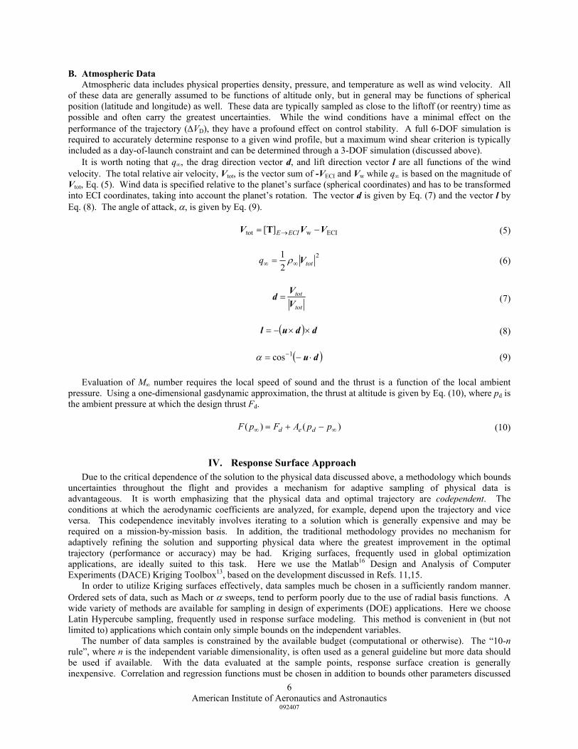
B. Atmospheric Data Atmospheric data includes physical properties density, pressure, and temperature as well as wind velocity. All

of these data are generally assumed to be functions of altitude only, but in general may be functions of spherical position (latitude and longitude) as well. These data are typically sampled as close to the liftoff (or reentry) time as possible and often carry the greatest uncertainties. While the wind conditions have a minimal effect on the performance of the trajectory (ΔVD), they have a profound effect on control stability. A full 6-DOF simulation is required to accurately determine response to a given wind profile, but a maximum wind shear criterion is typically included as a day-of-launch constraint and can be determined through a 3-DOF simulation (discussed above).

It is worth noting that q∞, the drag direction vector d, and lift direction vector l are all functions of the wind velocity. The total relative air velocity, Vtot, is the vector sum of -VECI and Vw while q∞ is based on the magnitude of Vtot, Eq. (5). Wind data is specified relative to the planet’s surface (spherical coordinates) and has to be transformed into ECI coordinates, taking into account the planet’s rotation. The vector d is given by Eq. (7) and the vector l by Eq. (8). The angle of attack, α, is given by Eq. (9).

ECIwtot ][ VVV −= →ECIET (5)

2

21

totq V∞∞ = ρ (6)

tot

tot

VVd = (7)

( ) ddul ××−= (8) ( )du ⋅−= −1cosα (9)

Evaluation of M∞ number requires the local speed of sound and the thrust is a function of the local ambient pressure. Using a one-dimensional gasdynamic approximation, the thrust at altitude is given by Eq. (10), where pd is the ambient pressure at which the design thrust Fd.

)()( ∞∞ −+= ppAFpF ded (10)

IV. Response Surface Approach Due to the critical dependence of the solution to the physical data discussed above, a methodology which bounds

uncertainties throughout the flight and provides a mechanism for adaptive sampling of physical data is advantageous. It is worth emphasizing that the physical data and optimal trajectory are codependent. The conditions at which the aerodynamic coefficients are analyzed, for example, depend upon the trajectory and vice versa. This codependence inevitably involves iterating to a solution which is generally expensive and may be required on a mission-by-mission basis. In addition, the traditional methodology provides no mechanism for adaptively refining the solution and supporting physical data where the greatest improvement in the optimal trajectory (performance or accuracy) may be had. Kriging surfaces, frequently used in global optimization applications, are ideally suited to this task. Here we use the Matlab16 Design and Analysis of Computer Experiments (DACE) Kriging Toolbox13, based on the development discussed in Refs. 11,15.

In order to utilize Kriging surfaces effectively, data samples much be chosen in a sufficiently random manner. Ordered sets of data, such as Mach or α sweeps, tend to perform poorly due to the use of radial basis functions. A wide variety of methods are available for sampling in design of experiments (DOE) applications. Here we choose Latin Hypercube sampling, frequently used in response surface modeling. This method is convenient in (but not limited to) applications which contain only simple bounds on the independent variables. The number of data samples is constrained by the available budget (computational or otherwise). The “10-n rule”, where n is the independent variable dimensionality, is often used as a general guideline but more data should be used if available. With the data evaluated at the sample points, response surface creation is generally inexpensive. Correlation and regression functions must be chosen in addition to bounds other parameters discussed


092407

7

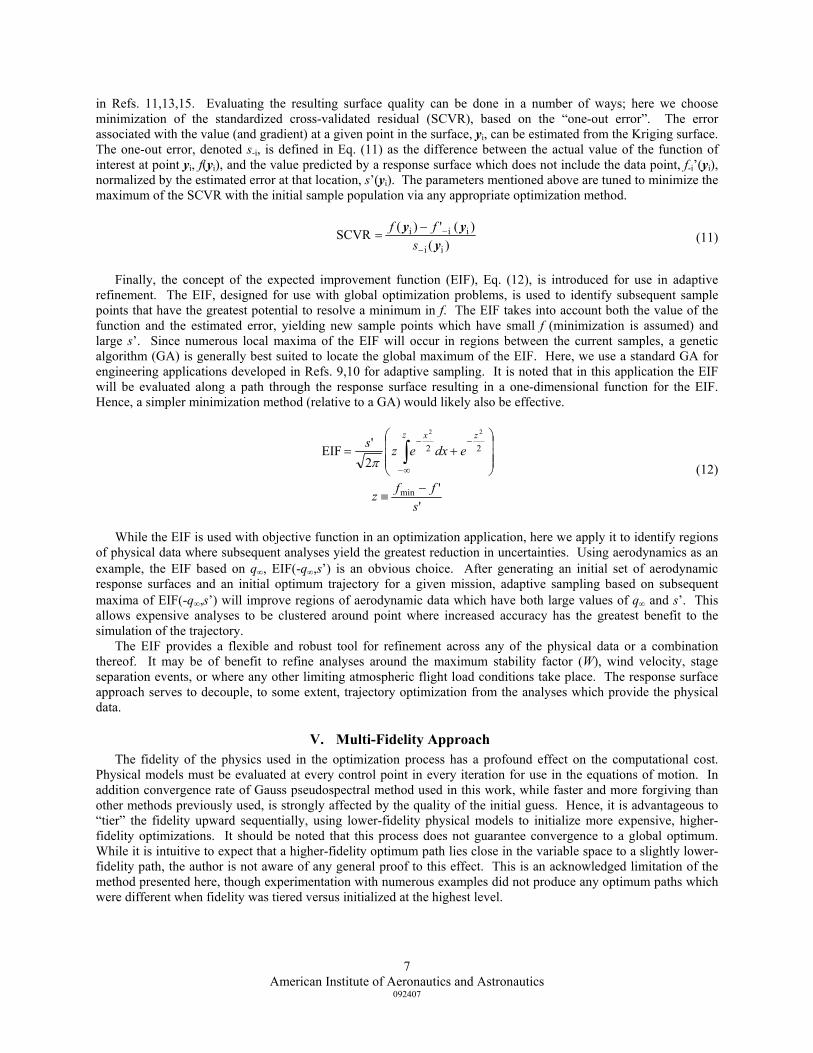
in Refs. 11,13,15. Evaluating the resulting surface quality can be done in a number of ways; here we choose minimization of the standardized cross-validated residual (SCVR), based on the “one-out error”. The error associated with the value (and gradient) at a given point in the surface, yi, can be estimated from the Kriging surface. The one-out error, denoted s-i, is defined in Eq. (11) as the difference between the actual value of the function of interest at point yi, f(yi), and the value predicted by a response surface which does not include the data point, f-i’(yi), normalized by the estimated error at that location, s’(yi). The parameters mentioned above are tuned to minimize the maximum of the SCVR with the initial sample population via any appropriate optimization method.

)()(')(SCVR

ii

iii

yyy

−

−−=

sff (11)

Finally, the concept of the expected improvement function (EIF), Eq. (12), is introduced for use in adaptive refinement. The EIF, designed for use with global optimization problems, is used to identify subsequent sample points that have the greatest potential to resolve a minimum in f. The EIF takes into account both the value of the function and the estimated error, yielding new sample points which have small f (minimization is assumed) and large s’. Since numerous local maxima of the EIF will occur in regions between the current samples, a genetic algorithm (GA) is generally best suited to locate the global maximum of the EIF. Here, we use a standard GA for engineering applications developed in Refs. 9,10 for adaptive sampling. It is noted that in this application the EIF will be evaluated along a path through the response surface resulting in a one-dimensional function for the EIF. Hence, a simpler minimization method (relative to a GA) would likely also be effective.

⎟⎟⎟

⎠

⎞

⎜⎜⎜

⎝

⎛+=

−

∞−

−

∫ 22

22

2'EIF

zz x

edxezsπ

''min

sffz −

≡

(12)

While the EIF is used with objective function in an optimization application, here we apply it to identify regions of physical data where subsequent analyses yield the greatest reduction in uncertainties. Using aerodynamics as an example, the EIF based on q∞, EIF(-q∞,s’) is an obvious choice. After generating an initial set of aerodynamic response surfaces and an initial optimum trajectory for a given mission, adaptive sampling based on subsequent maxima of EIF(-q∞,s’) will improve regions of aerodynamic data which have both large values of q∞ and s’. This allows expensive analyses to be clustered around point where increased accuracy has the greatest benefit to the simulation of the trajectory. The EIF provides a flexible and robust tool for refinement across any of the physical data or a combination thereof. It may be of benefit to refine analyses around the maximum stability factor (W), wind velocity, stage separation events, or where any other limiting atmospheric flight load conditions take place. The response surface approach serves to decouple, to some extent, trajectory optimization from the analyses which provide the physical data.

V. Multi-Fidelity Approach The fidelity of the physics used in the optimization process has a profound effect on the computational cost. Physical models must be evaluated at every control point in every iteration for use in the equations of motion. In addition convergence rate of Gauss pseudospectral method used in this work, while faster and more forgiving than other methods previously used, is strongly affected by the quality of the initial guess. Hence, it is advantageous to “tier” the fidelity upward sequentially, using lower-fidelity physical models to initialize more expensive, higher-fidelity optimizations. It should be noted that this process does not guarantee convergence to a global optimum. While it is intuitive to expect that a higher-fidelity optimum path lies close in the variable space to a slightly lower-fidelity path, the author is not aware of any general proof to this effect. This is an acknowledged limitation of the method presented here, though experimentation with numerous examples did not produce any optimum paths which were different when fidelity was tiered versus initialized at the highest level.


092407

8

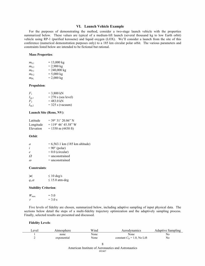
VI. Launch Vehicle Example For the purposes of demonstrating the method, consider a two-stage launch vehicle with the properties

summarized below. These values are typical of a medium-lift launch (several thousand kg to low Earth orbit) vehicle using RP-1 (purified kerosene) and liquid oxygen (LOX). We’ll consider a launch from the site of this conference (numerical demonstration purposes only) to a 185 km circular polar orbit. The various parameters and constraints listed below are intended to be fictional but rational.

Mass Properties: mS,1 = 13,000 kg mS,2 = 2,900 kg mP,1 = 240,000 kg mP,2 = 5,000 kg mPL = 2,000 kg

Propulsion: F1 = 3,800 kN Isp,1 = 270 s (sea level) F2 = 483.0 kN Isp,2 = 325 s (vacuum) Launch Site (Reno, NV): Latitude = 39° 31’ 20.86” N Longitude = 119° 46’ 45.58” W Elevation = 1350 m (4430 ft) Orbit: a = 6,563.1 km (185 km altitude) i = 90° (polar) e = 0.0 (circular) Ω = unconstrained ω = unconstrained Constraints: |w| ≤ 10 deg/s q∞α ≤ 15.0 atm-deg Stability Criterion: Wmax = 5.0 τ = 3.0 s Five levels of fidelity are chosen, summarized below, including adaptive sampling of input physical data. The sections below detail the steps of a multi-fidelity trajectory optimization and the adaptively sampling process. Finally, selected results are presented and discussed. Fidelity Levels:

Level Atmosphere Wind Aerodynamics Adaptive Sampling 1 none None None No 2 exponential None constant CD = 1.0, No Lift No


092407

9

3 exponential Response Surfaces constant CD = 1.0, No Lift Yes 4 MSISE-90 splines Response Surfaces Response Surfaces Yes 5 MSISE-90 splines Response Surface Response Surfaces N/A

A. Aerodynamic Response Surface Creation Here, we will assume aerodynamic coefficients CD and CL are given by analytical expressions Eqs. (13) and (14) respectively. This allows the response surface estimation to be compared directly to the function, but it is worth emphasizing that this would not be possible in general. Note that Eqs. (13-14) has finite, positive limits as M∞ → 0 and M∞ → ∞. Note that we have implicitly assumed an axisymmetric vehicle and neglected the dependence of CD and CL on Re.

⎟⎟⎠

⎞⎜⎜⎝

⎛

+−+−

=∞∞

∞∞

1.0421.9140.30490.71270.4750)cos(C 2

2

D MMMMα (13)

⎟⎟⎠

⎞⎜⎜⎝

⎛

+−+++

=∞∞∞

∞∞

1.629528.6593.946.081317.050.94)sin(80C 23

2

L MMMMMα (14)

The aerodynamic response surfaces must be generated as if the Eqs. (19-20) were unknown functions. With no a priori knowledge of the path taken through {M∞,α} space, an initial sample of 50 points (CFD solutions or wind tunnel tests) is used and the function is sampled via Latin Hypercube over the range 0 < α < 10° and 0 < M∞ < 3.0. The resulting initial response surfaces, resulting from a minimization of the SCVR as discussed above, are plotted in Figs. (1-2) against the exact functional forms. Details of the response surfaces are summarized below. If CFD data were used, these response functions could correspond to inviscid or viscous solutions depending on the level of fidelity desired for the initial estimate. Since the fidelity levels listed above do not make any distinction between the fidelity of the aerodynamic data itself, we’ll assume these are evaluated at the highest level of fidelity.

Figure 1. Comparison of CD response surface (right) with Eq. (13), (left). Note significant inaccuracies in CD throughout the domain shown due to the strong dependence on M∞.


092407

10

Figure 2. Comparison of CL response surface (right) with Eq. (14), (left). CL is very smooth and nearly linear in α for small α resulting in a close comparison with the initial sample.

B. Wind Data Response Surface Creation A fictional but representative set of balloon-sampled wind data was used for the purposes of this case study, plotted below in Figs. (3). It was assumed that wind is horizontal and its magnitude and direction are a function only of altitude. All data were sampled in altitude increments of approximately 0.25 km up to a maximum altitude of approximately 22.0 km. Above this altitude, the wind velocity held constant in magnitude at the maximum altitude sample value while the direction was held constant at the average value. A one-dimensional response “surface” was created using the Kriging method discussed above for Vw(h) and the wind direction. It is worth noting that balloon-based wind measurement typically must include some accounting for persistence, or the extent to which the measured profile changes with time, but this is presently neglected.

Figure 3. Wind speed (left) and direction (right) for the representative profile with +/- three s’ range (red) from one-dimensional response surface. In this simple case, local maxima occur between each data point.


092407

11

C. Atmospheric Data Typically, ρ∞(h), p∞(h), and T∞(h) would be sampled from balloon data in addition to the wind data discussed above. Here, for the purposes of simplicity, we assume the MSISE-90 model8,12,18. Many models are available for various regions of the atmosphere; the MSISE-90 model is well-suited for applications spanning a large range in altitude. These we implemented by fitting and subsequently evaluating cubic splines over the range 0 km < h < 200 km. Low-fidelity ρ∞(h) and p∞(h) distributions were taken as exponential, Eqs. (15-16). The scale height was taken as a constant 7.3 km based on sea-level data in Ref. 20, but various with altitude in general. It is noted that T∞ can vary substantially in the upper atmosphere depending on solar and seasonal conditions but here is only used for the computation of the speed of sound. Above approximately 40 km, the density and hence q∞ are low enough that errors in the speed of sound (and hence M∞) have a small impact on the resulting optimum trajectory but a continuous evaluation of M∞ is helpful for numerical performance. The ideal gas equations of state was used to compute the speed of sound from T∞ based on a constant γ = 1.4.

Shhe /SL

−∞ = ρρ (15)

Shhepp /SL

−∞ = (16)

Figure 4. Density (left) and temperature (right) profiles from the MSIS-E-908,12,18 model up to 200 km.

D. Results Optimizations were performed at each level of fidelity, initializing each new level of fidelity from the previous solution. Additional data points were adaptively sampled based on EIF(-q∞,s’) until the adaptive sampling budget of 20 points on the aerodynamic response surfaces was exhausted. Selected paths through {M∞,α} space are shown in Fig. (5) and EIF results, based on the original CD and CL response surfaces for consistency, are shown in Fig. (6). Results of the high-fidelity optimum are shown in Fig. (7).


092407

12

Figure 5. Mach-α flight profiles for various levels of fidelity. Note that M∞ actually decreases in certain flight regimes due to an increasing speed of sound. Fidelity levels which utilize wind data have α (t0) = 90° due to the vertical liftoff constraint. Note that much of the flight is spent at α > 10°, the maximum used in the initial response surface data range.

Figure 6. EIF(-q∞,s’) results for CD and CL during flight, based on the original (unadapted) response surfaces shown in Figs. (1-2) above. Note that EIF values are lower during the portion of the flight covered by the M∞ range of the initial response surfaces and increases in regions of high α. Fidelity level 1, which does not include wind, dramatically alters the α profile and hence the EIF values. Note that CD EIF values are much larger due to the relatively poor fit representation provided by the CD response surface.


092407

13

Figure 7. Optimum trajectory results from highest fidelity level simulation: total airspeed velocity (including wind), upper left, control vector components in ECI coordinates, upper right, altitude (lower left), and dynamic pressure with α, lower right. Stage division is visible in the velocity plot where a discontinuity exists in acceleration. Note that the optimum path in this particular case rises above the final altitude before adding speed via thrust with a downward component. These results are driven primarily by α (t), a function primarily of wind conditions. Note that the initial range, 0 < α < 10°, was too small for the lower-M∞ portion of the flight. This observation emphasizes the usefulness of the EIF as a tool for adaptively sampling. Simply adding points in the region of maximum q∞ would, in this example, be of little value in increasing the fidelity of the solution overall. By taking into account the estimated error as well, additional data can be tuned to regions of interest for a particular mission. As M∞ becomes large late in the flight, decreasing q∞ competes with rapidly increasing error (recall the original upper limit of M∞ was 3.5), resulting in large values of the EIF.

VII. Conclusions & Future Directions A multi-fidelity, response surface based trajectory optimization tool was developed and tested with an ascent

trajectory example. By initializing higher levels of fidelity with the solutions of lower fidelity optimization and adaptively sampling physical data in independent variable regions of greatest impact, high-fidelity optima can be determined with minimal computational cost or solution time. Since atmospheric conditions are typically sampled shortly before liftoff and continuously change, rapid determination of launch availability can be critical to the mission success. Here, accuracy very close to that of a solution utilizing exact aerodynamic data was achieved with a small number of samples relative to increasing the sampling resolution of the entire variables space.

There are numerous future directions to improve the capability studied here. A key improvement is the generalization to 6-DOF, requiring a control system model. The rotational degrees of freedom have physical time scales << the orbital time scale used in a 3-DOF simulation resulting in a stiff set of ODEs. This presents numerous problems to numerical optimization methods, the least of which is the number of control points required for adequate resolution of the independent rotational states. Practically, the rotational states must be driven by guidance which is a function of state. Since GPOCS does not rely on shooting (integrating the ODEs forward in time), feedback control can be implemented with appropriate transient behavior.

Accounting for the rotational DOFs also required a complete set of aerodynamic data, including pitch, yaw, and roll moments. This increases the dimensionality of the response surface needed for aerodynamic performance, placing additional emphasis on adaptive sampling for efficient high-fidelity results. The simplified stability criterion


092407

14

used here would be replaced with more accurate measures of controllability for day-of-launch criteria evaluation. Depending on the control system used, this may result in more EIF objectives for adaptive sampling.

Finally, extending the physical disciplines to include other results of interest to ascent and reentry trajectories would increase the usefulness of an EIF-based approach to adaptive refinement. These would include flight environments such as heat transfer and structural dynamics (natural modes). Path or endpoint constraints on stagnation point heat transfer or dynamic amplification, for example, could be included with the supporting physics and subsequently adaptively refined for a given mission based on any combination of criteria. Structural dynamic response can be particualry sensitive to payload mass properties, making adaptive refinement in this area particularly useful in mission planning especially if a source for unsteady aerodynamic prediction were available.

Acknowledgments The author would like to thank Marcus Edvall and Anil Rao of Tomlab Optimization, Inc. for their support and

advice with the GPOCS package used for dynamic optimization in this work.

References 1Bryson, A. E., Applied Linear Optimal Control, Cambridge University Press, 2002. 2Bryson, A. E., Dynamic Optimization, Addison-Wesley, 1999. 3Bensen, D. A., Huntington, G. T., Thorvaldsen, T. P., and Rao, A. V., “Direct Trajectory Optimization and Costate Estimation via an Orthogonal Collocation Method”, Journal of Guidance, Control, and Dynamics, Vol. 29, No. 6, Nov-Dec. 2006. 4Betts, J. T., “Survey of Numerical Methods for Trajectory Optimization”, Journal of Guidance, Control, and Dynamics, Vol. 21, N o. 2, 1998, pp. 193-207. 5Betts, J. T., Practical Methods for Optimal Control Using Nonlinear Programming, SIAM Press, Philadelphia, 2001. 6Gill, P. E., Murray, W., and Saunders, M. A.,"SNOPT: An SQP Algorithm for Large-Scale Constrained Optimization," SIAM Review, Vol. 47, No. 1, 2005, pp. 99-131. 7Hargraves, C. R., and Paris, S. W., “Direct Trajectory Optimization Using Nonlinear Programming and Collocation”, Journal of Guidance, Control, and Dynamics, Vol. 10, No. 4, 1987, pp. 338-342. 8Hedin, A. E., “Extension of the MSIS Thermospheric Model into the Middle and Lower Atmosphere”, Journal of Geophysical Research, Vol. 96, No. A2, pp. 1159–1172, 1991. 9Holst, T. L. and Pulliam, T.H., “Evaluation of Genetic Algorithm Concepts Using Model Problems, Part I: Single Objective Optimization”, NASA/TM-2003-212812, 2003. 10Holst, T. L. and Pulliam, T.H., “Evaluation of Genetic Algorithm Concepts Using Model Problems, Part II: Multi-Objective Optimization”, NASA/TM-2003-212813, 2003. 11Jones, D. R., Schonlau, M., and Welch, W.J., “Efficient Global Optimization of Expensive Black-Box Functions”, Journal of Global Optimization, Vol. 33, 2005. 12Labitzke, K., Barnett, J. J., and Edwards, B. (editors), Handbook MAP 16, SCOSTEP, University of Illinois, Urbana, 1985. 13Lophaven, S. N., Nielsen, H.B., and Søndergaard, J., “DACE: A Matlab Kriging Toolbox”, Version 2.0, Technical Report IMM-TR-2002-12, Technical University of Denmark, 2002. 14Ross, I. M., Fahroo, F., “A Perspective on Methods for Trajectory Optimization”, AIAA/AIS Astrodynamics Specialist Conference and Exhibit, Aug. 2002. 15Sóbester, A., Leary, S.J., and Keane, A. J., “On the Design of Optimization Strategies Based on Global Response Surface Approximate Models”, Journal of Global Optimization, Vol. 13, 1998. 16Matlab, Software Package, Ver. 7.5.0, MathWorks, Inc., 2007.


092407

15

17NIMA TR8350.2: "Department of Defense World Geodetic System 1984, Its Definition and Relationship with Local Geodetic Systems." 3rd ed., July, 1997. 18NSSDC (Goddard Space Flight Center) ModelWeb MSISE-90 Model: http://nssdc.gsfc.nasa.gov/space/model/atmos/msise.html 19TOMLAB, Software Package, Ver. 5.9, Tomlab Optimization, 2007. 20“U.S. Standard Atmosphere”, U.S. Government Printing Office, Washington, D.C., 1976.

Multi-Fidelity Trajectory Optimization with Response...

Documents

Transcript of Multi-Fidelity Trajectory Optimization with Response...