Multi Currency Credit Default Swaps - Quanto effects …dbrigo/QuantSummit2016.pdfMulti Currency...

Multi Currency Credit Default Swaps

Quanto effects and FX devaluation jumps

Prof. Damiano BrigoDept. of Mathematics

Mathematical Finance Group & Stochastic Analysis GroupImperial College London

Joint work with Nicola Pede and Andrea Petrelli

Quant Summit Europe

London, 13 April 2016

Introduction: Credit Default Swaps and Technical Setting

1 Introduction: Credit Default Swaps and Technical SettingDefault Risk: reduced form / intensity credit risk modelsCDS

2 Financial Motivation: CDS in multiple currenciesThe Italy CDS example

3 Mathematical framework for multi-currency CDSMulti-currency pricingFX rate dynamics and symmetriesQuanto survival probabiltiesDefault intensity modelInstantaneous correlation FX/Credit SpreadsPricing equationsInstantaneous correlation not enough for Default-FX contagionAdding jump-to-default FX contagion to explain the currency basisDirect Default-FX contagion and impact on CDS spreadsA numerical study of Italy’s CDS in EUR and USD

4 Conclusion

(c) 2015 Prof. Damiano Brigo with N. Pede, A. Petrelli Multi Currency CDS London, 13 April 2016 2 / 30

Introduction: Credit Default Swaps and Technical Setting Default Risk: reduced form / intensity credit risk models

Default: Reduced-form intensity modelling & Cox process

Let us consider a probability space (Ω,G,Q, (Gt)) satisfying the usual hypothesis and aprocess (λt, t > 0), the intensity, defined on this space. Let Λ(s) =

∫s0 λudu.

Default is a jump process (Dt, t > 0) with the property that λt is the Gt−intensity of D. Weonly focus on the first jump time of D and we call it τ, the default time.

Let us consider

the filtration generated by λ and “default-free processes" (eg short rate rt), (Ft);

the filtration generated by D, Ht = σ((τ < u),u 6 t) (“default monitoring")

separable filtration assumption: Total filtration Gt = (Ft)∨ (Ht);

a r.v. ξ ∼ exp(1) “jump to default risk", that is independent of (Ft).

Let us defineτ := Λ−1(ξ)

assuming λ > 0. From the default time definition we get that

Q(τ ∈ [t, t+ dt)|τ > t,Ft) = λt dt, (λt dt is a “local default probability");

Q(τ > T |Ft) = E

Q( ∫T0λs ds < ξ

∣∣∣∣∣FT)|Ft

= E[e−

∫T0 λs ds|Ft

](λ also “credit spread").


Introduction: Credit Default Swaps and Technical Setting CDS

Credit Defaul Swaps

A CDS is a contract between two parties A and B written with respect to a set of securitiesissued by the reference entity C where

before default of the reference entity or until a final maturity, one party [protectionbuyer] pays the other [protection seller] a protection premium; this can be paid upfront,running or both;upon default of the reference entity, if this happens before the final maturity, theprotection seller pays the buyer a loss given default on the reference entity’s securities.

A B

Premium: S

LGD

For a running CDS with premium spread Sc, the premium and the protection leg cash flowsdiscounted back at time 0 and not yet present valued are given respectively by

ΠPremium = ScN∑i=0

1τ>TiαiDccy(0, Ti)+accrual-term, ΠProtection = LGD1τ6TND

ccy(0, τ)

where accrual-term =Sc(τ− Tcoupon before τ)Dccy(0, τ)1τ<TN and

(T0, . . . , TN) quarterly spaced payment times, αi year fraction between Ti−1 & Ti;Dccy(t, T) stochastic discount factor for currency ccy at time t for maturity T ;


Financial Motivation: CDS in multiple currencies

Multi-currency CDS

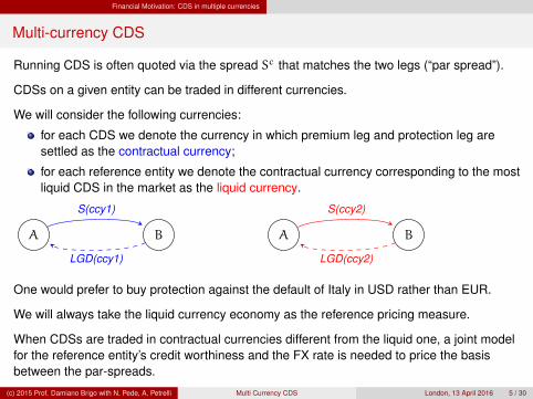
Running CDS is often quoted via the spread Sc that matches the two legs (“par spread”).

CDSs on a given entity can be traded in different currencies.

We will consider the following currencies:

for each CDS we denote the currency in which premium leg and protection leg aresettled as the contractual currency;

for each reference entity we denote the contractual currency corresponding to the mostliquid CDS in the market as the liquid currency.

A B A B

S(ccy1)

LGD(ccy1)

S(ccy2)

LGD(ccy2)

One would prefer to buy protection against the default of Italy in USD rather than EUR.

We will always take the liquid currency economy as the reference pricing measure.

When CDSs are traded in contractual currencies different from the liquid one, a joint modelfor the reference entity’s credit worthiness and the FX rate is needed to price the basisbetween the par-spreads.


Financial Motivation: CDS in multiple currencies The Italy CDS example

A look at the marketItaly’s case

1 Italy’s CDS in EUR:contractual currency: EURliquid currency: USD

2 Italy’s CDS in USD:contractual currency: USDliquid currency: USD

May 2011 Sep 2011 Jan 2012 May 2012 Sep 2012 Jan 2013 May 2013 Sep 20130

100

200

300

400

500

600

Spre

ads

(bps)

S 5YEUR

S 5YUSD


Mathematical framework for multi-currency CDS

1 Introduction: Credit Default Swaps and Technical SettingDefault Risk: reduced form / intensity credit risk modelsCDS

2 Financial Motivation: CDS in multiple currenciesThe Italy CDS example

3 Mathematical framework for multi-currency CDSMulti-currency pricingFX rate dynamics and symmetriesQuanto survival probabiltiesDefault intensity modelInstantaneous correlation FX/Credit SpreadsPricing equationsInstantaneous correlation not enough for Default-FX contagionAdding jump-to-default FX contagion to explain the currency basisDirect Default-FX contagion and impact on CDS spreadsA numerical study of Italy’s CDS in EUR and USD

4 Conclusion


Mathematical framework for multi-currency CDS Multi-currency pricing

Mathematical framework for multi-currency pricing

We will consider the case where the contractual and liquid currencies are different.Consider

a risk neutral measure Q with numeraire (Bt, t > 0) with

dBt = r(t)Bt dt, B0 = 1

is associated to the liquid currency:

a risk-neutral measure Q with numeraire (Bt, t > 0) where

dBt = r(t)Bt dt, B0 = 1

is associated to the contractual currency;

an exchange rate (Zt, t > 0) between the currencies of the two economies (Z is theprice of one unit of the contractual currency in the liquid currency);

interest rates are deterministic functions of time, although we will keep notationgeneral in view of generalizations


Mathematical framework for multi-currency CDS Multi-currency pricing

Mathematical framework for multi-currency pricing

Recall: B contractual currency, B liquid currency.The link between the two measure is provided by the Radon-Nikodym derivativeLT := dQ

dQ |GT. This can be calculated using a change of numeraire argument and a generic

function φT representing a payoff denominated in the liquid currency. The price of the liquid

currency payoff φ is then Et[BtBTφT

], satisfying the usual

1Zt

Et[Bt

BTφT

]= Et

[Bt

BT

φT

ZT

]⇒ Et

[Bt

BTφT

]= Et

[BtZt

BTZTφT

]= Et

[BtZt

BTZTφTdQdQ∣∣GT

]“First discount liquid, then price liquid, then change to contractual==first change to contractual, then discount contractual, then price contractual"The liquid-ccy expectation can be rewritten also as

Et[Bt

BTφT

]= Et

[BtBTZT

BT BtZt

BtZt

BTZTφT

].

From there, we can deduce the Radon-Nikodym derivative to be

Lt =ZtBt

Z0Bt, L0 = 1,


Mathematical framework for multi-currency CDS FX rate dynamics and symmetries

FX rates no-arbitrage dynamics

The fact that (Lt, t > 0) is a G-martingale in Q can be used to deduce no-arbitrageconstraints. For example, if r and r are deterministic functions of time and if (Zt, t > 0) is aGBM

dZt = µZZt dt+ σZt dWt, Z0 = z,

we can deduce the dynamics of the Radon-Nikodym derivative L as

dLt = d

(Bt

Bt

Zt

Z0

)=

Bt

BtZ0(dZt + rZt dt− rZt dt),

=Bt

BtZ0(µZZt dt+ σZt dWt + rZt dt− rZt dt), L0 = 1.

The martingale condition on L is given by Et [dLt] = 0, from which we can deduce the FXdrift rate:

µZ = r(t) − r(t)


Mathematical framework for multi-currency CDS FX rate dynamics and symmetries

Symmetry for FX rates

What if we had started from dQdQ |GT

and from the reciprocal FX rate, (Xt, t > 0) whereX = 1/Z, instead?

If (Zt, t > 0) (or X) are GBM, it doesn’t matter which RN derivative we start from. If, forexample, we first start from L, from which we calculate the no-arbitrage drift for Z asabove (r− r), we subsequently deduce X’s dynamics though Ito’s formula for 1/Z, andwe finally use Girsanov’s theorem to move X’s dynamics under the measure Q, weobtain

µX = r(t) − r(t)

This is the same drift we would have obtained postulating a GBM for X and deriving itsdrift starting from dQ

dQ |GT.

The same cannot be guaranteed to happen for other type of stochastic process for Zor X (e.g. stoch vol in FX, CEV...).


Mathematical framework for multi-currency CDS Quanto survival probabilties

Quanto survival probabilities

We start from the price of defaultable zero-coupon bond:

Et

[Bt

BT1τ>T

]= Et

[Bt

BT1τ>T

dQdQ

]=

This can be written as

=B(t, T)Zt

Et [ZT1τ>T ] (∗),

where B(t, T) = D(t, T) = Bt/BT is the discount factor from time T to time t 6 T .Remember we are assuming deterministic risk free discount rates.We define the quanto-adjusted survival probability as

pt(T) :=Et[Bt

BT1τ>T

]B(t, T)

We will often use (Ut, t > 0)

Ut := ZtEt

[Bt

BT1τ>T

]= by(∗)above = B(t, T)Et [ZT1τ>T ]

which is therefore a Q-price and as such has drift rUdt.


Mathematical framework for multi-currency CDS Default intensity model

Default intensity modelling

Although for credit spreads the square root processes are better in terms of tractability andclosed form solutions (B. et al [2, 3]), for lognormal consistency in this work we model theintensity λ under the liquid measure Q as an exponential Ornstein-Uhlenbeck process

λt = eYt

dYt = a(b− Yt)dt+ σY dWYt Y0 = y,

which leads to the default time τ = Λ−1(ξ), ξ ∼ exp(1) and recall

λ is instantaneous credit spread, λtdt local default probability in [t, t+ dt);

ξ is jump to default risk.

Dependence between the credit component and the FX component is modeled thoughinstantaneous correlation, ρ,

dZt = µZZtdt+ σZZt dWZt , Z0 = z;

d〈WY ,WZ〉t = ρ dt


Mathematical framework for multi-currency CDS Instantaneous correlation FX/Credit Spreads

Impact of correlation

Example: CDS on Italy, EUR=Contractual ccy, USD= liquid ccy.

Z is the amount of USD needed to get one unit of EUR.

If ρ negative⇒ intensity tends to grow when FX rate Z decreases.

When λ ↑ default of Italy becomes more likely and the amount of USD needed to getone EUR will tend to decrease (EUR devaluation), so that the EUR protection offeredby the CDS will be worth less when benchmarked against the liquid USD CDS

This results in a lower par spread for the EUR CDS.

Positive correlation will lead to a larger par spread.

More generally, ceteris paribus, we expect the par spread to increase with thecorrelation.


Mathematical framework for multi-currency CDS Pricing equations

The pricing equation

The dependency of survival probability value of the default event that is given by theadditional process Dt = 1τ<t must be explicitly considered. (Ut, t > 0) can berepresented as some function f(t,Xt, Yt,Dt) and we have (Itô’s lemma with jumps)

dUt = rf dt+ ∂tf dt+ ∂zf(µZz dt+ σZz dWZ

t

)+ ∂yf

(a(b− Yt) dt+ σY dWY

t

)+

12

(σZz

)2∂zzf dt+

12

(σY)2∂yyf dt+ ρσZσYz∂zyf dt+ ∆f dDt,

where ∆f = f(t, x,y, 1) − f(t, x,y, 0) is the jump to default of the survival probability. Towrite the pricing equation, it has to be noted that D is not a martingale, so its compensatormust be calculated. The process (Mt, t > 0) given by

Mt = Dt −

∫ t0(1−Ds)λs ds (1)

is a G-martingale in Q.Imposing that the drift of dU to be rUt = rf yields




∂tf+ µZz∂zf+ a(b− Yt)∂yf+

12

(σZz

)2∂zzf

+12

(σY)2∂yyf+ ρσ

ZσYz∂zyf+ ey(1− d)∆f = 0,

The PDE for f can be solved it in two steps:1 calculating first u(t, x,y) := f(t, x,y, 1);2 using u to solve for v(t, x,y) := f(t, x,y, 0)

They only get coupled through the term ey(1− d)∆f and that term only enters thev−equation. Final conditions for the two functions are respectively given by

v(T , z,y) = f(T , z,y, 0) = z;

u(T , z,y) = f(T , z,y, 1) = 0

(see Jeanblanc et al [1] for a more general discussion).



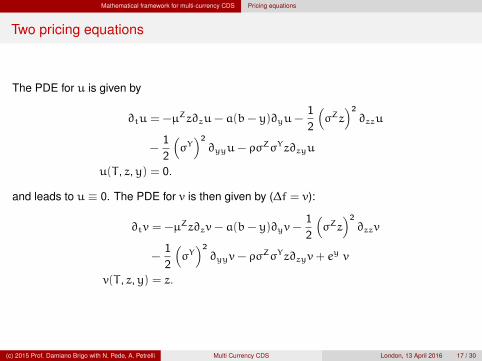
Two pricing equations

The PDE for u is given by

∂tu = −µZz∂zu− a(b− y)∂yu−12

(σZz

)2∂zzu

−12

(σY)2∂yyu− ρσZσYz∂zyu

u(T , z,y) = 0.

and leads to u ≡ 0. The PDE for v is then given by (∆f = v):

∂tv = −µZz∂zv− a(b− y)∂yv−12

(σZz

)2∂zzv

−12

(σY)2∂yyv− ρσ

ZσYz∂zyv+ ey v

v(T , z,y) = z.




u and v can be interpreted as pre-default and post-default values of a derivative with payofffunction φ:

f(t, x,y,d) = Et[φ(XT , YT ,DT )|Xt = x, Yt = y,Dt = d

]= 1τ>tEt

[φ(XT , YT ,DT )|Xt = x, Yt = y,Dt = 0

]+ 1τ6tEt

[φ(XT , YT ,DT )|Xt = x, Yt = y,Dt = 1

]= 1τ>tv(t, x,y) + 1τ6tu(t, x,y)

We will solve numerically the PDEs by using an Alternating Directions Implicit schemevariant, accurate fourth order in x and second order in t (see [6]).


Mathematical framework for multi-currency CDS Instantaneous correlation not enough for Default-FX contagion

Limits of instantaneous correlation on Quanto CDS par spreads S

1.0 0.5 0.0 0.5 1.0

ρ

6

4

2

0

2

4

6

S(ρ,σY

)−S(ρ

=0,σY

) (b

ps)

σY =0.2

0.20 0.25 0.30 0.35 0.40 0.45 0.50 0.55 0.60

σY

10

15

20

25

30

35

S(ρ

=1,σY

)−S(ρ

=−

1,σY

) (b

ps)

z µ σZ a b y T

0.8 0.0 0.1 0.0001 204.0 -4.089 5.0

Italy CDS. Contractual currency: EUR. Liquid Currency: USD. We see that even the maximumexcursion of correlation cannot explain the discrepancy between CDS spreads in two currencies, since

differences in the markets can reach much larger ranges than what we see here (case of Italy).(c) 2015 Prof. Damiano Brigo with N. Pede, A. Petrelli Multi Currency CDS London, 13 April 2016 19 / 30

Mathematical framework for multi-currency CDS Direct Default-FX contagion and impact on CDS spreads

Adding Jump to default: Direct Default-FX contagion

We can account for the devaluation factor directly in the dynamics of (Zt, t > 0) byconsidering

dZt = µZZt dt+ σZZt dWZt + γZt− dDt , Z0 = z,

Take again the example of Italy.

Now, if Italy defaults, a negative γ would push Z down with a jump.

The amount of USD needed to buy 1 EUR jumps down, we have a intantaneousdevaluation jump for the EUR, which makes sense in a scenario of default of Italy.

As a consequence the CDS offering protection in EUR will be worth much less whenbenchmarked with that in USD, so that we expect the par spread to go down with anegative γ.

A less negative or positive γ would instead give us a larger par spread.

We expect the par spread to increase with γ.



Adding Jump to default: Direct Default-FX contagion

Re-doing calculations as above but accounting for the new jump term in Z:

dUt = rf dt+∂tf dt+∂zf(µZz dt+ σZz dW

(2)t + γZz dDt

)+∂yf

(a(b− Yt) dt+ σY dW

(1)t

)+

12

(σZz

)2∂zzf dt+

12

(σY)2∂yyf dt+ ρσZσYz∂zyf dt+ ∆f dDt − ∂zf∆Zt.

The pricing equation associated to that is

∂tv = −(r− r)z∂zv− a(b− y)∂yv−12

(σZz

)2∂zzv

−12

(σY)2∂yyv− ρσ

ZσYz∂zyv+ ey (v− γZz∂zv)

v(T , z,y) = z,



Hazard rate’s dyamics in Q

So far we always worked in the benchmark liquid currency measure Q.However there is an important approximation where we can benefit from deriving thecontractual currency measure Q dynamics for the intensity. By Girsanov’s theorem:

dMt = dMt −d〈M,L〉tLt

= dMt − d〈D,γZD〉t

= dMt − (1−Dt)γZλt dt

= dDt − (1−Dt)(1+ γZ)λt dt

from which the intensity of the default process in Q is given by

λt = (1+ γZ)λt

This is important because there are cases when a CDS par-spread can be suitablyapproximated by S ≈ (1− R)λ (e.g. deterministic constant hazard rate models). In suchcases, dividing both sides by LGD=1-R, which is fixed at the same level in both currenciesby the auction (Doctor et al. (2010) [5]), an approximated relation can be written for thepar-spreads of the contractual and liquid CDSs as

S = (1+ γZ)S



FX SymmetryJump diffusion

Requiring that (Lt, t > 0) is a G-martingale in Q leads to

µZ = r(t) − r(t) − λtγZ1τ>t

The dynamics in Q of (Xt, t > 0) can be calculated starting from the dynamics of(Zt, t > 0)

dXt = (r− r)Xt dt− σZXt dWZt + Xt−γ

X dMt, X0 =1z,

where

γX = −γZ

1+ γZ

That is a dynamics such that dQdQ |Gt

is a G-martingale in Q.


Mathematical framework for multi-currency CDS A numerical study of Italy’s CDS in EUR and USD

Jump to default effect on quanto spreads

−1.0 −0.5 0.0 0.5 1.0−6

−4

−2

0

2

4

6

∆S (

bps)

γ=0

−1.0 −0.5 0.0 0.5 1.0−62.0

−61.5

−61.0

−60.5

−60.0

−59.5

−59.0

−58.5

−58.0

−57.5

γ=0.6

−1.0 −0.5 0.0 0.5 1.0

ρ

−81.0

−80.5

−80.0

−79.5

−79.0

−78.5

∆S (

bps)

γ=0.8

−1.0 −0.5 0.0 0.5 1.0

ρ

−106

−104

−102

−100

−98

−96

−94

γ=1

∆S := S(ρ,γ) − S(0, 0)

z µ σZ a b y σY T

0.8 0.0 0.1 0.0001 -210.0 -4.089 0.2 5.0



Jump to default effect on default probabilities

We can link the ratio of quanto-adjusted and single-currency default probabilities and thefactor γ. For

small Tthe two are linked by

1+ γ =1− pt(T)1− pt(T)

−1.0 −0.8 −0.6 −0.4 −0.2 0.0

γZ

0.0

0.2

0.4

0.6

0.8

1.0

1.2

1−p(T)

1−p(T)

T=1

T=3

T=5

T=10

Figure: Low spread (≈ 100bps)

−1.0 −0.8 −0.6 −0.4 −0.2 0.0

γZ

0.0

0.2

0.4

0.6

0.8

1.0

1−p(T)

1−p(T)

T=1

T=3

T=5

T=10

Figure: High spreads, (≈ 700bps).



CDS spreads on Italy in 2011-2013



CDS spreads on Italy in 2011-2013Linking parameters to market data

Let us recall the change in intensity of default induced by the JTD in the Radon-Nikodymderivative:

λt = (1+ γZ)λt

This relation can be inverted and used as a way to estimate γ from market data.

−0.40 −0.35 −0.30 −0.25 −0.20 −0.15 −0.10 −0.05

S 1YEUR−S 1Y

USD

S 1YUSD

−0.5

−0.4

−0.3

−0.2

−0.1

0.0

0.1

γ

Figure: Relative basis spread for 1Y maturityCDSs.

−0.40 −0.35 −0.30 −0.25 −0.20 −0.15 −0.10 −0.05

S 5YEUR−S 5Y

USD

S 5YUSD

−0.5

−0.4

−0.3

−0.2

−0.1

0.0

0.1

γ

Figure: Relative basis spread for 5Y maturityCDSs.


Conclusion

Conclusions

Throughout this presentation we showed

a model that can consistently accounts both for instantaneous correlation between FXand hazard rate and for a devaluation effect;

that jump-to-default effects in FX rates are needed to account for observed quantobasis in the market;

how the introduction of jump to default in the RN derivative affects the intensity of thedefault event in different measures;

that introducing jump to default effects in the FX rate dynamics does not break the“symmetry”;

Numerical example and a practical recipe to estimate devaluation effect on FX fromCDS data.


Conclusion

References I

[1] Bielecki, T. R., Jeanblanc M. and M. Rutkowski.Pde approach to valuation and hedging of credit derivatives.Quantitative Finance, 5, 2005.

[2] Brigo, D., Alfonsi, A.,Credit Default Swap Calibration and Derivatives Pricing with the SSRD StochasticIntensity Model, Finance and Stochastic (2005), Vol. 9, N. 1.

[3] D. Brigo, and El-Bachir, N. (2010).An exact formula for default swaptions’ pricing in the SSRJD stochastic intensitymodel. Mathematical Finance, Volume 20, Issue 3, July 2010, Pages: 365-

[4] D. Brigo, N. Pede, and A. Petrelli (2015).Multi Currency Credit Default SwapsSSRN, http://papers.ssrn.com/sol3/papers.cfm?abstract_id=2703605.

[5] A. Elizalde, S. Doctor, and H. Singh (2010).Trading credit in different currencies via quanto CDS. Technical report, J.P. Morgan,October 2010. Retrieved on April 10, 2016 onhttp://www.wilmott.com/messageview.cfm?catid=11&threadid=97137


http://papers.ssrn.com/sol3/papers.cfm?abstract_id=2703605

Conclusion

References II

[6] Düring, B., Fournié, M. and A. Rigal (2013).High-order ADI schemes for convection-diffusion equations with mixed derivativeterms. In: Spectral and High Order Methods for Partial Differential Equations -ICOSAHOM’12, M. Azaiez et al. (eds.), pp. 217-226, Lecture Notes in ComputationalScience and Engineering 95, Springer, Berlin, Heidelberg, 2013

[7] Pykhtin, M. and Sokol, A. (2013).Exposure under systemic impact. Risk Magazine.

[8] P. Ehlers and P. Schönbucher.The Influence of FX Risk on Credit Spreads.Working Paper, ETH, 2006.

[9] D. Lando.Credit Risk Modeling – Theory and ApplicationsPrinceton Series in Finance, 2004.


Multi Currency Credit Default Swaps - Quanto effects …dbrigo/QuantSummit2016.pdfMulti Currency...

Documents

Transcript of Multi Currency Credit Default Swaps - Quanto effects …dbrigo/QuantSummit2016.pdfMulti Currency...