Multi-Continuum Approach to Modeling Shale Gas...

Multi-Continuum Approach to Modeling Shale GasExtraction

Anna Russian · Philippe Gouze · MarcoDentz · Alain Gringarten

Abstract Production rates in horizontal shale gas wells display declines that arecontrolled by the low permeability and the intrinsic heterogeneity of the shalematrix. We present an original multi-continuum approach that yields a physicalmodel able to reproduce the complexity of the decreasing gas rates. The modeldescribes the dynamics of gas rate as function of the physical reservoir parametersand geometry, while the shale matrix heterogeneity is accounted for by a stochasticdescription of transmissivity field. From the D = 3 dimensional problem setting,including the heterogeneous shale matrix, the fractures generated by the hydro-fracking operations, as well as the production well characteristics, we establish aneffective upscaled 1D model for the gas pressures in fracture and matrix as well asthe volumetric flux. We analyse the decline curves behaviour and we identify thetime scales that characterize the dynamics of the gas rate decline using explicitanalytical Laplace space solutions of the upscaled process model. Asymptoticallythe flux curves decrease exponentially, while in an intermediate regime we find apower law behaviour, in which the flux scales with a power-law in time as t−β ,where β reflects the medium heterogeneity. We use this solution to fit a set of realdata displaying distinctly different decline trends and study the sensitivity of themodel to the reservoir parameters in order to identify their respective controls atthe different stages of the decline curve dynamics. Results indicate that the initialvalue of the gas rate is determined by the transmissivity of the fractures and theinitial pressure of the gas in the shale matrix. The latter causes mainly a shift of theentire decline curve. The early time of decline curve shape is primarily controlled

Anna RussianGeosciences, Universite de Montpellier 2, CNRS, Montpellier, France.Tel.: +33 467149315E-mail: [email protected]

Philippe GouzeGeosciences, Universite de Montpellier 2, CNRS, Montpellier, France.

Marco DentzInstitute of Environmental Assessment and Water Research (IDAEA), Spanish National Re-search Council (CSIC), Barcelona, Spain.

Alain GringartenCentre for Petroleum Studies, Imperial College London (ICL), London, United Kingdom.

2 A. Russian et al.

by the fracture properties (compressibility and transmissivity). During the mainpart of the economically valuable production times, i.e. before the production ratedrops exponentially, the decline curve is strongly controlled by the properties ofthe shale-rocks including their heterogeneity, which is modeled by two parametersdescribing the non-Fickian pressure diffusion effects in a stochastic framework.

Keywords Shale Gas · Modeling · Multi-continuum Model · Shale Reservoirs

1 Introduction

Shale gas has become an increasingly important source of natural gas. Shale gasreservoirs contain a large portion of the remaining gas reserves in the world, butare less developed in comparison with conventional gas. The main characteristic ofshale gas reservoirs is that they exhibit extremely low matrix permeability. Mod-elling the dynamic behaviour of shale gas extraction is particularly challengingbecause the problem includes a variety of physical and chemical processes interre-lated at different scales. Moreover, the spatial heterogeneity triggered by frackingoperations brings complexity in the gas flow dynamics while the extremely tightformations give rise to long asymptotic decreasing flowrate in the gas productionthat cannot be explained by classical linear models.

Most of the commonly used methods derive from the pioneer work of Arps,developed for conventional reservoir [1]. Arps rate time model and successive ex-tensions quantify the decline behaviour in terms of the Arps decline exponentb. Decline curve analysis is one of the oldest and most used diagnostic tool ofpetroleum engineer. Arps-derived methods are popular for analyzing decline curvesbecause they require only a ’best fit’ with the measured gas rate. However, the useof Arps rate decline equations for unconventional reservoirs often over estimatesreserves. The b values obtained by fitting gas production data are greater than 1,resulting in unrealistic production forecasts with rates that never approach zero.This issue has been widely discussed, e.g. [2,3], and new models have been pro-posed to avoid these physically unreasonable results, for instance by considering atransient productivity index e.g. [4–6].

Generally, gas production is characterized by successive different regimes: aftera first initial regime often difficult to predict because it depends by many differentprocesses (fracturing, flow-back of the water used to fracking, etc), gas entersthe effective production regime where the gas flow through a system of micro-fracture thought the extraction well. During this transient regime the gas rateproduction curve decreases following different scaling behaviour till it achieves thefinal regime where the gas production rate decrease exponentially [7]. A limitationof the models mentioned above, is that the development of different flow regimes isdifficult to predict which limits their utility for long-term production predictions.Specifically the transient regime preceding the exponential decrease is controlledby coupled effects of both the fractures and the shale matrix properties and candisplay distinctly different trends.

The aim of this work is to obtain a simplified but effective description of thedynamics of gas production at observation scale, tightly linked to the underlyingprocesses at lower scales. This upscaled model allows extracting the critical infor-mation on the reservoir characteristics, which can be used for predicting long-term

Multi-continuum Model for Shale Gas 3

behaviour. Considering the manifest uncertainty on the actual processes and thephysical parameters that control the dynamic of gas the extraction, many authorshave focused their efforts on developing models as simple as possible.

For instance [8] stated that gas production follows a nearly universal functionscaled by only two parameters. The total amount of gas in place and an charac-teristic fracture interference time, i.e., the time for a pressure pulse to propagatebetween two planar hydrofracture. The op. cit. model [8] is a non-linear homoge-neous diffusion model. It predicts that after few months of production, the recov-ery rate scales as t−1/2 until a given characteristic time after which it decreasesexponentially. This is the classical behavior observed in dual continuum modelsfor linear solute transport or two-phase flow in highly heterogeneous media [25,24]. However, there are many examples, as those studied in this paper, of ratecurves which do not display the t−1/2 decline. Yet, shale gas reservoir are natu-rally heterogeneous and we can anticipate that this heterogeneity must be takeninto account for explaining the distinctly different rate curves observed. Moreoverwe note that the total amount of gas, one of the two parameters of the op. cit.model of [8], is rarely known a priori.

The aim of the present paper is to propose a model that represent the complex,3D heterogeneous reservoir response with a simplified 1-dimensional linear model,where heterogeneity is handled within a stochastic framework. Specifically, wederive an upscaled multi-continuum model that can explain the long decliningrates observed in the analysis of gas shale production

The model is based on the widely used dual porosity approach which is apriori meaningful for such a dual system containing hydraulic discontinuities inless permeable matrix. In dual porosity reservoir models, the shale matrix is theportion of the reservoir that can store large quantities of gas, but displays lowconductivity that hamper transporting the gas over long distances. Conversely,the fractures, which partition the matrix, is the main vector for transporting thegas toward the extraction well, for instance. But the fractures have a limitedpotential for storage.

In conventional reservoir the fractured network can pre-exist (naturally frac-tured reservoir) but in shale gas reservoirs, the fracture clusters, constituted byfracture, micro-fracture, cracks and natural fractures re-opened, are generatedby multiple stages of hydraulic fracturing around horizontal wells [9]. After thefracking stages, the gas diffuses to the production well through the network offractures, which is recharged by diffusion from the matrix elements. Since thepioneering work of [10], a number of double permeability/porosity models havebeen developed (e.g. [11–15]) and have been extended to gas production problemeven considering heterogeneous matrix (e.g. [16–20]). These models assume thatboth fractures and matrix elements are in quasi-equilibrium and mass transfer ismodelled as a first order process. Linear reservoir models that take into accounttransient matrix-fracture transfer have been derived in Laplace space by [12,21]and extended by [22].

Here we consider non-equilibrium effects in the matrix triggered by its het-erogeneity. Mass exchanges between the fracture system and the heterogeneousmatrix give rise to non-integer exponents of the rate-decline slopes and, as anevidence, allow modeling a large range of rate-production data. Transient matrix-fracture transfers are controlled by a matrix memory kernel which is defined bythe properties of the matrix only. On the other hand we reduce the complexity

4 A. Russian et al.

of the problem by considering diffusion in the matrix linear, even though it is,in principle, non-linear. Notice that the validity of linearization of the diffusionproblem in the matrix has been favorably discussed in [23–25].

The underlying conceptual model is illustrated schematically in Figure 1. InSection 2, we describe the multi-continuum model, derive the constitutive upscaledeffective equations and then give an analytical solution for the pressure and thegas flowrate in the Laplace space. In Section 3 we test this multi-continuum modelto actual gas production from a shale gas formation, which displays dissimilar de-creasing rate curves. The objective of these examples is to illustrate the ability ofthe model to explain distinctly different behaviours by the intrinsic properties ofthe reservoir.Then, we study the sensitivity of the model to the reservoir parame-ters and identify the set of parameter that primarily control the dynamics of thedeclining flowrate. Conclusions are given in Section 4.

2 Multi-Continuum Model

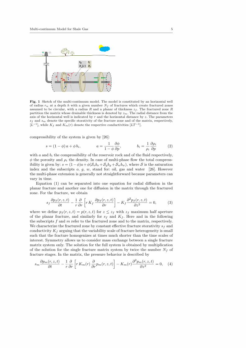
The model relies on the idea that the gas, initially trapped in the matrix, can bedrained by the fractured zone after hydraulic fracturing and diffuse toward thehorizontal part of the extraction well. Thus, one can identify two main processes:(i) the refilling of the fractured zone by the matrix, and (ii) the migration of thegas to the extraction points through the fractured zone. Figure 1 illustrates theconceptual model. The model is constituted by a horizontal well at a given depthwith a number of vertical fractures (Nf ) perpendicular to the well. Each fracturestage is associated to a planar fractured zone, which is characterized by a higherconductivity compared to the surrounding matrix, where the gas is trapped.

The aim is to start from the d = 3 dimensional radial conceptual model given inFig. 1 and upscale it into a d = 1 dimensional equivalent one by using spatial andensemble averaging. We handle the spatial heterogeneity of the matrix stochas-tically, with spatially varying conductivities model as spatial random fields. Weconsider a stationary and ergodic medium with a finite correlation, so that themedium can be completely defined by a single point distribution for an observa-tion scale much larger than the correlation scale.

2.1 Model Derivation

2.1.1 Statement of the problem

The governing equation for the pressure in the model sketched in figure 1 reads inradial coordinates [26]:

s(z)∂p(r, z, t)

∂t− 1

r

∂

∂r

»r K(r, z)

∂p(r, z, t)

∂r

–− ∂2[K(r, z) p(r, z, t)]

∂z2= 0, (1)

where p(r, z, t) is the pressure in radial coordinates (r, z) at time t, with rw ≤ r ≤R, s(z) is the effective compressibility of the system and K is given by K = k/µwith k the permeability of the system and µ the viscosity of the gas. The effective


Fig. 1 Sketch of the multi-continuum model. The model is constituted by an horizontal wellof radius rw at a depth h with a given number Nf of fractures which create fractured zonesassumed to be circular, with a radius R and a planar of thickness zf . The fractured zone Rpartition the matrix whose drainable thickness is denoted by zm. The radial distance from theaxis of the horizontal well is indicated by r and the horizontal distance by z. The parameterssf and sm denote the specific storativity of the fracture zone and of the matrix, respectively,

[L−1], while Kf and Km(r) denote the respective conductivities [LT−1].

compressibility of the system is given by [26]:

s = (1− φ) a + φ bi, a =1

1− φ

∂φ

∂p, bi =

1

ρi

∂ρi

∂p(2)

with a and bi the compressibility of the reservoir rock and of the fluid respectively,φ the porosity and ρi the density. In case of multi-phase flow the total compress-ibility is given by: s = (1−φ)a+φ(Sobo +Sgbg +Swbw), where S is the saturationindex and the subscripts o, g, w, stand for: oil, gas and water [26]. Howeverthe multi-phase extension is generally not straightforward because parameters canvary in time.

Equation (1) can be separated into one equation for radial diffusion in theplanar fracture and another one for diffusion in the matrix through the fracturedzone. For the fracture, we obtain

sf∂pf (r, z, t)

∂t− 1

r

∂

∂r

»r Kf

∂pf (r, z, t)

∂r

–−Kf

∂2pf (r, z, t)

∂z2= 0, (3)

where we define pf (r, z, t) = p(r, z, t) for z ≤ zf with zf maximum half apertureof the planar fracture, and similarly for sf and Kf . Here and in the followingthe subscripts f and m refer to the fractured zone and to the matrix, respectively.We characterize the fractured zone by constant effective fracture storativity sf andconductivity Kf arguing that the variability scale of fracture heterogeneity is smallsuch that the fracture homogenizes at times much shorter than the time scales ofinterest. Symmetry allows us to consider mass exchange between a single fracturematrix system only. The solution for the full system is obtained by multiplicationof the solution for the single fracture matrix system by twice the number Nf offracture stages. In the matrix, the pressure behavior is described by

sm∂pm(r, z, t)

∂t− 1

r

∂

∂r

»r Km(r)

∂

∂rpm(r, z, t)

–−Km(r)

∂2pm(r, z, t)

∂z2= 0, (4)

6 A. Russian et al.

where sm, pm(r) and Km(r) indicate respectively effective compressibility, pres-sure and permeability over viscosity in the matrix for zf ≤ z ≤ zm and zm themaximum size of matrix influenced by the fracture.

At the interface between the fractured zone and the matrix, at z = zf , weimpose continuity of pressure and flux:

pf (r, zf , t) = pm(r, zf , t), Kf∂pf (r, z, t)

∂z

˛zf

= Km(r)∂pm(r, z, t)

∂z

˛zf

. (5)

Moreover we consider that the radial flux thought the external edge of the fractureis negligible because R indicates the radius of influence of the horizontal well whichdetermines the Stimulated Reservoir Volume (SRV). Gas trapped at a distancer > R from the horizontal well is not mobilized during production [8]. Thus,we set a no-flux condition at the edge of the fracture, Kf [∂pf (r, z, t)/∂r]r=R =0. The same boundary condition is imposed in the matrix domain at z = zm,Km(r)[∂pm(r, z, t)/∂z]z=zm = 0.

The permeability in the fracture is much larger than the permeability in thematrix, thus Kf � max{Km(r)}. Therefore, equilibrium along the z directionin the fracture is reached relatively faster than in the matrix and we can suitablyassume pf (r, z, t) ' pf (r, t). Moreover, the difference in conductivity between frac-ture and matrix makes matrix diffusion preferably oriented in the direction of thefractures. Thus, neglecting radial diffusion in the matrix, the constitutive equationfor the matrix given in Eq. (4) reduces to:

sm∂pm(r, z, t)

∂t−Km(r)

∂2pm(r, z, t)

∂z2= 0. (6)

We assume that the matrix conductivity varies in radial direction. The matrix actsas a source term for the fractures as expressed by the continuity conditions (5).

2.1.2 Spatial average

In order to obtain a simpler effective description, we integrate the governing dif-fusion equation over the the coordinate z, and we reduce the d = 3 dimensionalradial problem into an effective d = 1 dimensional one. The average pressures inthe fracture and in the matrix are defined as

pf (r, t) =1

zf

zfZz0

dz pf (r, z, t), pm(r, t) =1

zm

zm+zfZzf

dz pm(r, z, t). (7)

By executing spatial average of Eq. (3), as defined in 7, over the fracture aperturezf , gives:

Sf

∂pf (r, t)

∂t− 1

r

∂

∂rrTf

∂pf (r, t)

∂r= Km(r)

∂pm(r, z, t)

∂z

˛z=zf

, (8)

where we used the continuity condition (5) and we defined the total compressibilityof the fractured zone Sf = sfzf and the effective transmissivity Tf = Kfzf . Thelast term in Eq. (8) is the flux at the interface between fracture and matrix andit is obtained from the solution of the diffusion equation in the matrix, which is


given in Eq.(6). We solve Eq.(6) in the Laplace space with the following boundaryconditions: continuity of pressure pm(r, z, t) = pf (r, t) at z = zf and no fluxcondition boundary condition at z = zm. Notice that we set the fracture pressureat the interface equal to the cross-sectional average, which is justified becausethe vertical homogenization time over the fracture width tf = z2

fsf/Kf is muchsmaller than the characteristic matrix time scales.

Using the method of Green functions, we obtain the average pressure in thematrix as a function of the pressure in the fractured zone:

pm(r, t) =

Z t

0dτg[t− τ, τm(r)]pf (r, τ)

− pm(r, 0)

Z t

0dτg[τ, τm(r)] + pm(r, 0), (9)

with the uniform in z initial condition pm(r, t = 0) = pm(r, t = 0). The character-istic time scale for pressure propagation within the matrix is

τm(r) = z2msm/Km(r). (10)

In Eq. (9), pm(r, 0) is the initial pressure in the matrix and the matrix mem-ory kernel g(t, τm) is obtained by averaging the solution of Eq. (6) for the pulseboundary condition pm(r, z, t) = δ(t) at the interface z = zf . The function g(t, τm)is computed, for simplicity, in Laplace space. Laplace transform of g(t, τm), withrespect to the time t, reads as [27,28]:

g∗[λ, τm(r)] =1p

λτm(r)tanh

»qλτm(r)

–(11)

where λ is the Laplace variable and the asterisk denotes function in Laplace space.Laplace transform is defined in [29]. For times t � τm(r) the memory functiong(t, τm) decreases with time as g ∝ t−1/2, while it is cut-off exponentially fort > τm.

In order to obtain the flux term appearing on the right side of Eq. (8) as afunction of pf , we integrate along the z direction Eq.(6), we transform it in theLaplace space and we substitute pm as a function of pf according to Eq. (9). Thus,the spatial derivative on the right side of Eq. (8) reads in Laplace space as:

∂p∗m(r, z, λ)

∂z

˛z=zf

= −λzmsm

Kmg∗[λ, τm(r)]

»p∗f (r, λ)− pm(r, 0)

λ

–. (12)

Using this result in Eq.(8), we obtain the following non-local closed form equationfor the pressure in the fracture:

λ{Sf + Smg∗[λ, τm(r)]}p∗f (r, λ)− Tf

r

∂

∂rr∂p∗f (r, λ)

∂r=

Sfpf (r, 0) + Smg∗[λ, τm(r)]pm(r, 0) (13)

where Sm = smzm. Considering that at time zero t = 0 the fractured zone is inequilibrium with the matrix pf (r, 0) = pm(r, 0) the previous equation reduces to:

λ{Sf + Smg∗[λ, τm(r)]}p∗f (r, λ)− Tf

r

∂

∂rr∂p∗f (r, λ)

∂r=

{Sf + g∗[λ, τm(r)]}pf (r, 0). (14)

8 A. Russian et al.

Note that if one considers a homogeneous matrix, so that the model reducesto a double porosity medium, the memory function is time dependent only, i.e.g(t|r) ≡ g(t). The function g(t), obtained by solving Eq.(6) in Laplace space,represents the boundary matrix flux. One note that g(t) is equivalent to the Laplacetransform of the gas flux in the linearized model of [8].

In the following, we consider an heterogeneous matrix and thus we averagethe flux over the fracture-matrix boundary r. We use a stochastic approach be-cause we do not have a proper description of the heterogeneity distribution alongr. Accordingly, we describe the heterogeneity of the matrix by a distribution oftransition times, as described in the next section.

2.1.3 Ensemble average

In order to obtain an upscaled effective formulation for the multi-continuum model,we average the governing equation (13) over the heterogeneity of the matrix andwe obtain:

λ [Sf + ϕ∗(λ)] 〈p∗f (r, λ)〉 − Tf

r

∂

∂r

"r∂〈p∗f (r, λ)〉

∂r

#= [Sf + ϕ∗(λ)] 〈pf (r, 0)〉, (15)

where the squared brackets indicate the ensemble averaged quantities. In Eq. (15)we defined the global memory function as:

ϕ∗(λ) = 〈Smg∗[λ, τm(r)]〉, (16)

where the angular brackets indicate ensemble average over the distribution ofcharacteristic time scales τm(r). The global memory function for an heteroge-neous medium is given by the superposition of single memory functions g(t) forhomogeneous matrix.

In order to average Eq. (13) and obtain Eq. (15) we use the mean field approx-imation: D

ϕ∗(λ) p∗f (r, λ)E'˙ϕ∗(λ)

¸〈p∗f (r, λ)〉 (17)

which is pertinent for times at which the variation scale of the pressure in thefracture, pf , is larger than the heterogeneity scale of matrix. Note that this ap-proximation is done on a routine basis in similar multi-rate mass transfer (MRMT)models for solute transport in multi-continuum models [27,28]. The global mem-ory function defined in Eq. (16) is given by superposition of the local memoryfunctions n g(τ, t):

ϕ(t) = Sm

Z ∞

0P (τ) g(t, τ) dτ, (18)

where P (τ) is the probability density function of characteristic times τm, whichare related to the immobile conductivity K, through Eq. (10). The distribution ofcharacteristic time τm is expressed in terms of the distribution of Km, PK(k), as:P (τ) = z2

msm/τ2PK(z2msm/τ). A broad distribution of mass transfer scales may


be modeled by a truncated power law distribution of the trapping times in thematrix:

P (τ) =1− β

τ1−β2 − τ1−β

1

τ−β Θ(τ2 − τ) Θ(τ − τ1), (19)

where 1/2 < β < 1; τ1 and τ2 are the lower and upper limits of the truncatedpower law distribution, and Θ(·) is the Heaviside step function, which is equal toone if its argument is larger than zero and zero otherwise. We insert Eq. (19) inEq. (18) and, as shown in the Appendix A, we approximate the global memoryfunction by the following truncated power-law:

ϕ(t) =Sm

τ2Γ (1− β)

„t

τ2

«−β

exp

„− t

τ2

«, (20)

where Γ (·) denotes the gamma function. In Laplace space the memory functionreads as:

ϕ∗(λ) = Sm (λτ2 + 1)β−1 . (21)

From Eq.(15), we note that the power law distribution of τ controls the dynamic ofthe system when ϕ∗(λ) is larger that Sf . This condition identifies a characteristictime τa given by

τa = τ2

„Sf

Sm

« 11−β

, (22)

which corresponds to the activation time of the matrix. Specifically, it denotesthe time for which Sm(τa/τ2)

1−β = Sf . The influence of the truncated power lawdistribution of trapping time in the matrix is dominant for time t > τa. Note thatfor t < τa the model gives information on the fractured zone only and not onthe reservoir properties. Only for time t > τa the flux derived in the proposedmodel depends on the properties of the reservoir and then we can obtain differentbehaviour according to parameters of the matrix.

2.2 Solutions

In the following we solve Eq. (15) in Laplace space. The general solution of Eq. (15)is given by (see Appendix B for details):

〈p∗f (r, λ)〉 =ˆI1

`R′´K0

`r′´+K1

`R′´I0

`r′´˜

C∗(λ) +pf (0)

λ(23)

where I0(·) and K0(·) are the 0-th order modified Bessel functions of first andsecond kind respectively, I1(·) and K1(·) are the 1-st order modified Bessel func-tions of first and second kind; C∗(λ) is determined by the boundary conditions.We furthermore defined:

R′(λ) = Rq

τ ′(λ)λ, r′(λ) = rq

τ ′(λ)λ (24)

10 A. Russian et al.

τ ′(λ) =Sf + ϕ∗(λ)

Tf. (25)

In order to solve Eq. (15) and compute the C∗(λ) in Eq. (23), we note that theoutgoing flux, at r = rw, is proportional to the difference of pressure between thefractured zone and the well. Thus, we impose a Cauchy-type boundary conditionat the horizontal well

2πrwTf

"∂〈pf (r, t)〉

∂r

#r=rw

=1

α[〈pf (rw, t)〉 − pw(t)], r = rw (26)

"∂〈pf (r, t)〉

∂r

#r=R

= 0, r = R (27)

where α is the skin factor that relates the pressure drop with the flux of gasentering the horizontal well, and pw(t) is the pressure in the horizontal well. Atthe edge of the fractured zone, for r = R, we imposed a no-flux boundary conditionas discussed in Sect. 2.1.1. Thus, the function C∗(λ) in Eq.(23) is given by:

C∗(λ) = −pf (0)

λ − p∗w(λ)

I0 (r′w)K1 (R′) + I1 (R′)K0 (r′w) + A r′w [I1 (R′)K1 (r′w)− I1 (r′w)K1 (R′)],

(28)

where we define A = 2πTfα and, similarly as in Eq. (24),

r′w = rw

qτ ′(λ) λ. (29)

The flux of gas entering the horizontal well, Q(t), [L3T−1], is computed as theradial derivative of the pressure at r = rw and is given by:

Q(t) = −2πrwTf

"∂〈pf (r, t)〉

∂r

#r=rw

(30)

Hence, taking the radial derivative of Eq. (23), one obtains:

Q∗(λ) = 2πr′wTf

ˆI1

`R′´K1

`r′w´−K1

`R′´I1

`r′w´˜

C∗(λ). (31)

with C∗(λ) given in Eq. (28). Substituting expression (28) for C∗(λ) in the previousequation yields:

Q∗(λ) =2πr′wTf

hpf (r,0)

λ − p∗w(λ)i[I1(R

′)K1(r′w)−K1(R

′)I1(r′w)]

I0 (r′w)K1 (R′) + I1 (R′)K0 (r′w) + Ar′w [I1 (R′)K1 (r′w)− I1 (r′w)K1 (R′)].

(32)


2.3 Asymptotic behaviour

In order to depict the long time behaviour of the model we perform an asymptoticexpansion of (32) for the limit λτ ′ � 1. Thus, we obtain

Q∗(λ) ≈ τ ′(λ)πTf (R2 − r2w)∆p

1 + λτ ′(λ)h

R2

2 ln Rrw

+ A2 (R2 − r2

w)i (33)

as outlined in detail in Appendix C. Note that for simplicity we set the pressureat the well p∗w(λ) constant and ∆p = p0 − pw.

It is worth noticing that for times t � τ2, or equivalently for λτ2 � 1, thememory function ϕ∗(λ) → Sm. Thus, inserting this result in Eq. (25) we observedthat τ ′(λ) tends towards the constant value

τ ′(λ) → Sf + Sm

Tf. (34)

Moreover τ ′(λ) is also constant when ϕ∗(λ) � Sf or equivalently for t � τa (seeEq.(22)) . In this case, the flux comes from the fractured zone only, τ ′(λ) tendstowards the constant value

τ ′(λ) → Sf

Tf. (35)

and consequently the dynamic of the flowrate depends on the parameters of thefractured zone only. Accordingly, for the two time regimes defined by t � τ2

and t � τa the model behaves as an equivalent homogeneous model with τ ′(λ)constant and given by (34) and (35), respectively. For these regimes, it followsfrom the inverse Laplace transform of (33) that the flux behaves exponentially as

Q(t) ∼ exp(−t/τc), (36)

where the time scale τc is given by

τc =R2Sf

Tf

"1

2ln

R

rw+

A

2

1− r2

w

R2

!#(37)

for t � τa and by

τc =R2(Sf + Sm)

Tf

"1

2ln

R

rw+

A

2

1− r2

w

R2

!#(38)

for t � τ2.In the intermediate regime τa � t � τ2, the function τ ′(λ) behaves as

τ ′ ≈ Sm

Tf(λτ2)

β−1. (39)

By inserting this result in Eq.(33) one find that the Laplace transform of the fluxscales as Q∗(λ) ∝ (λτ2)

β−1. This implies that the flux in the intermediate timeregime decreases with the power-law behaviour

Q(t) ∝„

t

τ2

«−β

. (40)


a)

100 102 104 10610 1

100

101

102

103

104

105

106

time

Q(t)

tf

2 2 2

t

e t

b)

100 102 104 10610 1

100

101

102

103

104

105

106

time

Q(t)

2

t 0.7

tf

t 0.9

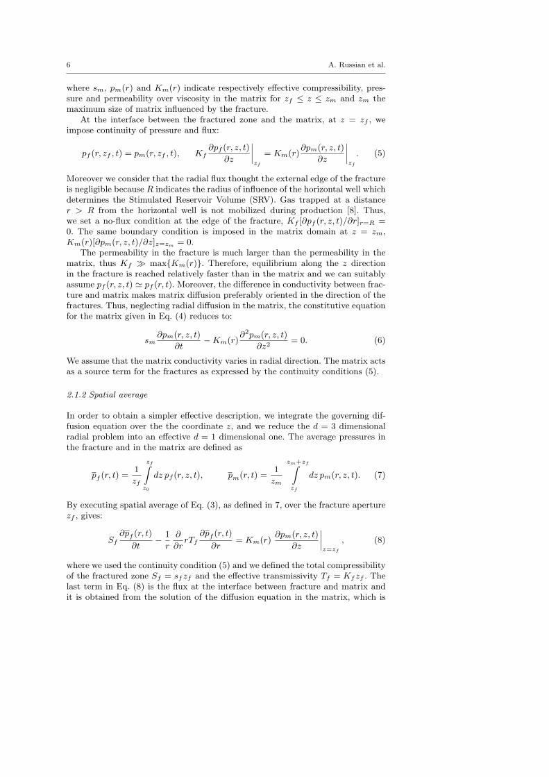
Fig. 2 Temporal evolution of flux as defined in Eq.32 for different values of the cutoff timeτ2 (Fig.2a) and different values of β (Fig.2b). Parameters: rw = 0.1m, Nf = 44, R = 25m,

Sf = 10−7 m/Pa, Tf = 2 ·10−9m3/Pa/s, ∆p = 3 ·107Pa, Sm = 10−6m/Pa,α=1 Kg/m3/s. For

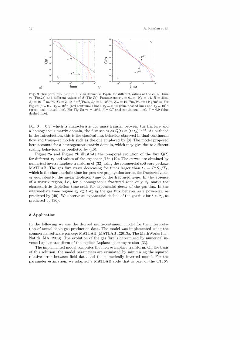
Fig.2a: β = 0.7, τ2 = 105d (red continuous line), τ2 = 104d (blue dashed line) and τ2 = 103d(green dash dotted line). For Fig.2b: τ2 = 105d, β = 0.7 (red continuous line), β = 0.9 (bluedashed line).

For β = 0.5, which is characteristic for mass transfer between the fracture anda homogeneous matrix domain, the flux scales as Q(t) ∝ (t/τ2)

−1/2. As outlinedin the Introduction, this is the classical flux behavior observed in dual-continuumflow and transport models such as the one employed by [8]. The model proposedhere accounts for a heterogeneous matrix domain, which may give rise to differentscaling behaviours as predicted by (40).

Figure 2a and Figure 2b illustrate the temporal evolution of the flux Q(t)for different τ2 and values of the exponent β in (19). The curves are obtained bynumerical inverse Laplace transform of (32) using the commercial software packageMATLAB. The gas flux starts decreasing for times larger than tf = R2Sf/Tf ,which is the characteristic time for pressure propagation across the fractured zone,or equivalently, the mean depletion time of the fractured zone. In the absenceof a matrix region, i.e., for a homogeneous fractured zone only, tf marks thecharacteristic depletion time scale for exponential decay of the gas flux. In theintermediate time regime τa � t � τ2 the gas flux behaves as a power-law aspredicted by (40). We observe an exponential decline of the gas flux for t � τ2, aspredicted by (36).

3 Application

In the following we use the derived multi-continuum model for the interpreta-tion of actual shale gas production data. The model was implemented using thecommercial software package MATLAB (MATLAB R2013a, The MathWorks Inc.,Natick, MA, 2013). The evolution of the gas flux is determined by numerical in-verse Laplace transform of the explicit Laplace space expression (33).

The implemented model computes the inverse Laplace transform. On the basisof this solution, the model parameters are estimated by minimizing the squaredrelative error between field data and the numerically inverted model. For theparameter estimation, we adapted a MATLAB code that is part of the CTRW


optimization Toolbox [31,32]. The code is based on the routine fminsearch imple-mented in MATLAB, which uses a Nelder-Mead simplex direct search algorithmto minimize the non-linear least squares objective function. The model allows es-timating the following parameters: the radius of the horizontal well rw, the meanradius of the zone of influence of the fracture stage R, the total compressibility ofthe fractured zone Sf = zfsf , the mean effective transmissivity of the fracturedzone Tf , the initial pressure of the reservoir p(0), the total compressibility of thematrix Sm = zmsm, the exponent of the power law distribution of transition timesin the matrix given in (19) β and its cut off τ2, the number of active fracturedzones Nf , the skin factor α. Because of the large number of fitting parameters, theinversion can be not unique. For this reason uncertainties are largely decreased ifa prior geological and/or physical information of the site are available in order tofix some parameters and, or, impose a pertinent range of variability on the others.A better knowledge of fracture properties from geophysical data will improve thebest fitting of the short time behavior, while (multi-scale) measurements of thematrix dispersivity will improve long term predictions. However these parametersare rarely analyzed and we believe that it is a major issue for reliable predictions.

3.1 Results

In this section we consider the gas flowrate of three production wells in Louisiana(US) for illustrating the use of the model. These wells display distinctly differentdecline curve shapes. As for many other data set, only few information about themedium properties are accompanying the decline curves. Possible modificationsof the well head configuration (e.g. change of the setup used to regulate the wellhead pressure) were not reported as well. Parameters for gas production of thethree production wells (noted hereafter A, B and C) are estimated, using as muchas possible the information available at this site. The gas flowrate is fitted (seeSection 3) by fixing the radius of the horizontal well rw and the number of fracturedstages Nf expected during the fracking stage. The depth at which the horizontalwell was drilled is known and can be used to evaluate the initial pressure (p0).

Due the large uncertainties on the well pressure value, we considered a constantflowing pressure in the well as the boundary condition pw(t) = pw in (26), andwe fit the difference of the initial reservoir pressure and the pressure in the well∆p = p(0)− pw. The results are shown in Figure 3 for well A and Figures 4a and4b for well B and C respectively.

Figure 3 displays the fit for well A gas flowrate with the multi-continuummodel (red solid line) and the curves related to equivalent homogeneous models.Similar plots are given for well B and C in figures 4. The proposed figures are inlog-log scale in order to highlight the asymptotic decreasing flowrate. An equiva-lent homogeneous model that represents the hydraulic properties of the fracturedzone only is obtained by setting ϕ∗(λ) = 0 in (15). An equivalent homogeneousmodel that comprises both the fractured and matrix domain is obtained by set-ting ϕ∗(λ) = Sm in (15). Note that in the asymptotic long time limit t � τ2,the memory function reduces to limt→∞ ϕ(t) = Smδ(t). The first case representsthe behaviour of the homogeneous fracture domain only, while the second caserepresents the the behaviour of an equivalent homogeneous system when fractureszone and matrix are in equilibrium. For the equivalent homogeneous cases, one can


101 102 103103

104

105

106

time (d)

gas flowrate (m3/d)

tm

tf

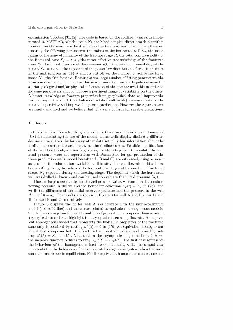
Fig. 3 Gas rate production of well A (blue dots) in log-log scale. Measurements are takendaily. Red line: Multi-continuum model fit. Violet line with squares: equivalent homogeneousmodel with ϕ = 0, Green line with triangles: equivalent homogeneous model with ϕ = Sm.Fixed parameters: rw = 0.09m, Nf = 44. Fitted parameters: R = 21.9m, Sf = 3.2·10−6 m/Pa,

Tf = 8.18 ·10−10m3/Pa/s, ∆p = 6.6 ·107Pa, Sm = 3.62 ·10−6m/Pa, b = 0.60, τ2 = 1.50 ·103d,

α=2.6 Kg/m4/s. Timescales: tf = R2Sf /Tf= 21.8d and tm = R2(Sf + Sm)/Tf = 46.35d.

observe that the gas flowrate deceases exponentially, see Appendix C. The data,however, displays a much slower decrease.

The multi-continuum model can properly fit the experimental data while thisis not possible with the equivalent homogeneous models whatever its parametriza-tion. The curves corresponding to the homogeneous models coincide with themulti-continuum model at short times but then decrease faster than what wouldbe required to reproduce the flowrate tailing. The curve representing the frac-ture domain only decreases exponentially fast for times larger than tf = R2Sf/Tf

which, as pointed out above, is the mean depletion time of the fractured zone. Thecurve representing the homogeneous equivalent to fractured and matrix domaindecreases exponentially fast for times larger than tm = R2(Sf +Sm)/Tf . This timescale represents the characteristic time to deplete both the fracture and matrixzones. These time scales are also reflected in characteristic scales (37) and (38).The multi-continuum model accounts for pre-asymptotic non-equilibrium betweenmatrix and fractured zones and yields a slowly decreasing asymptotic flowrate.

The parameters obtained by the fitting procedure are summarized in Table 1together with the root mean squared errors of the fits and the correlation coeffi-cients which quantify the good fit between the data and the model. The values ofthe skin factor α are not mentioned in the table because the data fits are unchangedby varying α in the range of values considered (see later discussion in Section 3.2).Similarly, the value of τ1 is not mentioned because it can be neglected as explainedin detail in Appendix A.

The values of the physical parameters obtained by the fitting procedure are inthe range of the typical values found in the literature for a shale reservoirs [33–35,8]. In the fitting process we impose a range of validity for some parameters suchas, for example, the radius of the fractured zone R that cannot be larger thanthe half thickness of the reservoir and some appropriate limits on compressibility,permeability and viscosity.


Data A B C

R, [m] 21.9 33.7 34.6Sf = zf sf , [m/Pa] 3.2 · 10−6 5.3 · 10−6 3.6 · 10−6

Tf = zfkµ

, [m3/Pa/s] 8.2 · 10−10 6.4 · 10−9 1.4 · 10−9

∆p = p0 − pw, [Pa] 6.6 · 107 8.2 · 106 3.6 · 107

Sm = zmsm, [m/Pa] 3.6 · 10−6 2.1 · 10−5 3.1 · 10−5

β 0.6 0.67 0.5τ2, [day] 1.5 · 103 6.4 · 102 4.9 · 104

tf , [day] 21.8 10.8 35.6tm, [day] 46.4 54.1 342RMSE 6.7 · 103 6.6 · 103 1.0 · 104

Corr 0.972 0.970 9.60

Table 1 Result fitted parameters. Parameters: R radius of the fractured zone, effective com-pressibility Sf = zf sf and Sm = zmsm with zf , zm thickness of the fractured zone andthe matrix, sf , sm compatibilities given by the soil and the gas compressibility (see Eq.(2)),Tf = zf k/µ with k permeability and µ viscosity at reservoir conditions, difference of initialpressure and pressure in the well ∆p = p0 − pw, exponent β and cut off τ2 of the powerlaw distribution of Eq.(21); RMSE is the root mean squared error and Corr is the correlationcoefficient.

a)10

110

210

3103

104

105

106

time (d)

gas flowrate (m3/d)

tf

tm

b)10

110

210

3104

105

106

time (d)

gas flowrate (m3/d)

tf

tm

Fig. 4 Gas Rate production of well B (on the left, Fig. 4a) and of well C (on the right,Fig. 4b). Field measurement (blue dots) are taken daily. Violet line with squares: equivalenthomogeneous model with ϕ = 0, green line with triangles: equivalent homogeneous model withϕ = Sm. Model parameters for well B (red line): fixed parameters: rw = 0.09 m, Nf = 45; fitted

parameters: R = 33.7 m, Sf = 5.3·10−6 m Pa−1, Tf = 6.4·10−9m3Pa−1s−1, ∆p = 8.2·106Pa,

Sm = 2.1 ·10−5m Pa−1, β = 0.67, τ2 = 6.38 ·102d, α = 24 Kg m−4s−1. Timescales for well B:tf = 10.8 d, tm = 54.1 d. Model parameters for well C (red line): fixed parameters: rw = 0.09m,

Nf = 48; fitted parameters: R = 34.6m, Sf = 3.6 · 10−6 m Pa−1, Tf = 1.4 · 10−9m3Pa−1s−1,

∆p = 3.6 · 107Pa, Sm = 3.1 · 10−5m Pa−1, β = 0.5, τ2 = 4.9 · 104d, α = 2.5 Kg m−4s−1.Timescales for well C: tf = 35.6 d, tm = 342.4 d.

3.2 Parameter Sensitivity

Here we perform a sensitivity analysis to evaluate the control level of each pa-rameter, or group of parameters, in the multi-continuum model. The sensitivityanalysis consists in changing on parameter while keeping the others fixed. We per-form this analysis starting from the parameter set best-fitted for well A (see Fig.3).Figure 5 displays the variation of the gas flowrate dynamic versus the radius of


a)101 102 103

103

104

105

106

time (d)

gas flowrate (m3/d)

Data Arw= 0.40

rw= 0.20

rw= 0.10

rw= 0.05

b)101 102 103

103

104

105

106

time (d)

gas flowrate (m3/d)

Data AR=32R=22R=17R=12

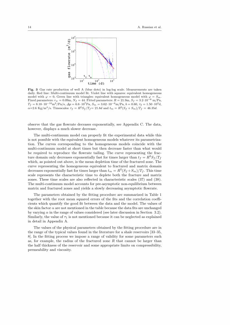
Fig. 5 Previous well A flowrate fit (Fig.3) for different values of the radius of the horizontalwell rw (on the left, Fig. 5a) and of the extension of the fractured zone R (on the right, Fig.5b). The values of rw and R are indicated in the figures and expressed in meters. Timescales:tf = 6.5 d for R = 12 m, tf = 13 d for R = 17 m, tf = 22 d for R = 22 m and tf = 46 d forR = 32 m. Values of the others parameters are given in the caption of Fig.3.

a)10

110

210

3103

104

105

106

time (d)

gas flowrate (m3/d)

Data ASf=1.0 10

5

Sf=3.0 10 6

Sf=1.0 10 6

Sf=1.0 10 7

b)10

110

210

3103

104

105

106

time (d)

gas flowrate (m3/d)

Data A

Tf=1.5 10 9

Tf=8.0 10

10

Tf=5.0 10 10

Tf=3.0 10 10

Fig. 6 Previous well A flowrate fit (Fig.3) for different values of the storativity of the fracturedzone Sf (on the left, Fig. 6a) and the transmissivity of the fractured zone Tf (on the right,

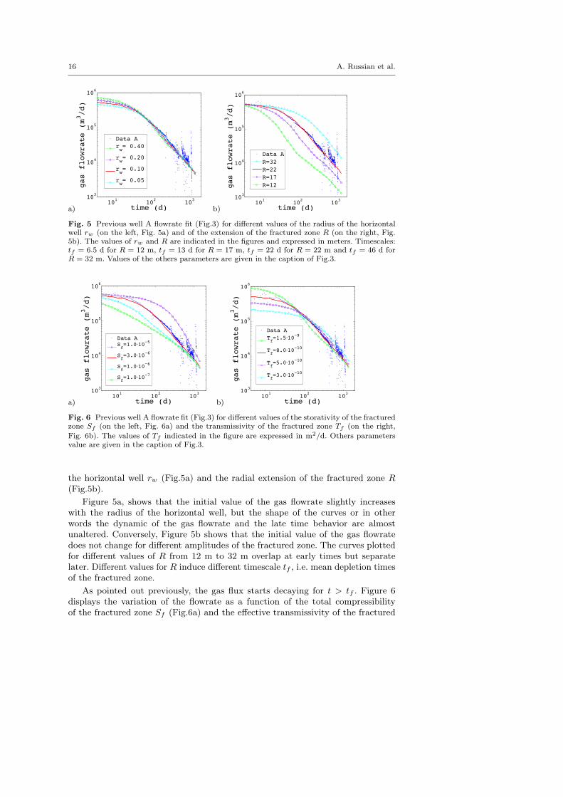
Fig. 6b). The values of Tf indicated in the figure are expressed in m2/d. Others parametersvalue are given in the caption of Fig.3.

the horizontal well rw (Fig.5a) and the radial extension of the fractured zone R(Fig.5b).

Figure 5a, shows that the initial value of the gas flowrate slightly increaseswith the radius of the horizontal well, but the shape of the curves or in otherwords the dynamic of the gas flowrate and the late time behavior are almostunaltered. Conversely, Figure 5b shows that the initial value of the gas flowratedoes not change for different amplitudes of the fractured zone. The curves plottedfor different values of R from 12 m to 32 m overlap at early times but separatelater. Different values for R induce different timescale tf , i.e. mean depletion timesof the fractured zone.

As pointed out previously, the gas flux starts decaying for t > tf . Figure 6displays the variation of the flowrate as a function of the total compressibilityof the fractured zone Sf (Fig.6a) and the effective transmissivity of the fractured


a)10

110

210

3103

104

105

106

time (d)

gas flowrate (m3/d)

Data ASm=1.0 10 5

Sm=4.0 10 6

Sm=1.0 10 6

Sm=4.0 10

7

b)101 102 103

103

104

105

106

time (d)

gas flowrate (m3/d)

Data A

p=1.0 106

p=7.0 107

p=5.0 107

p=3.0 107

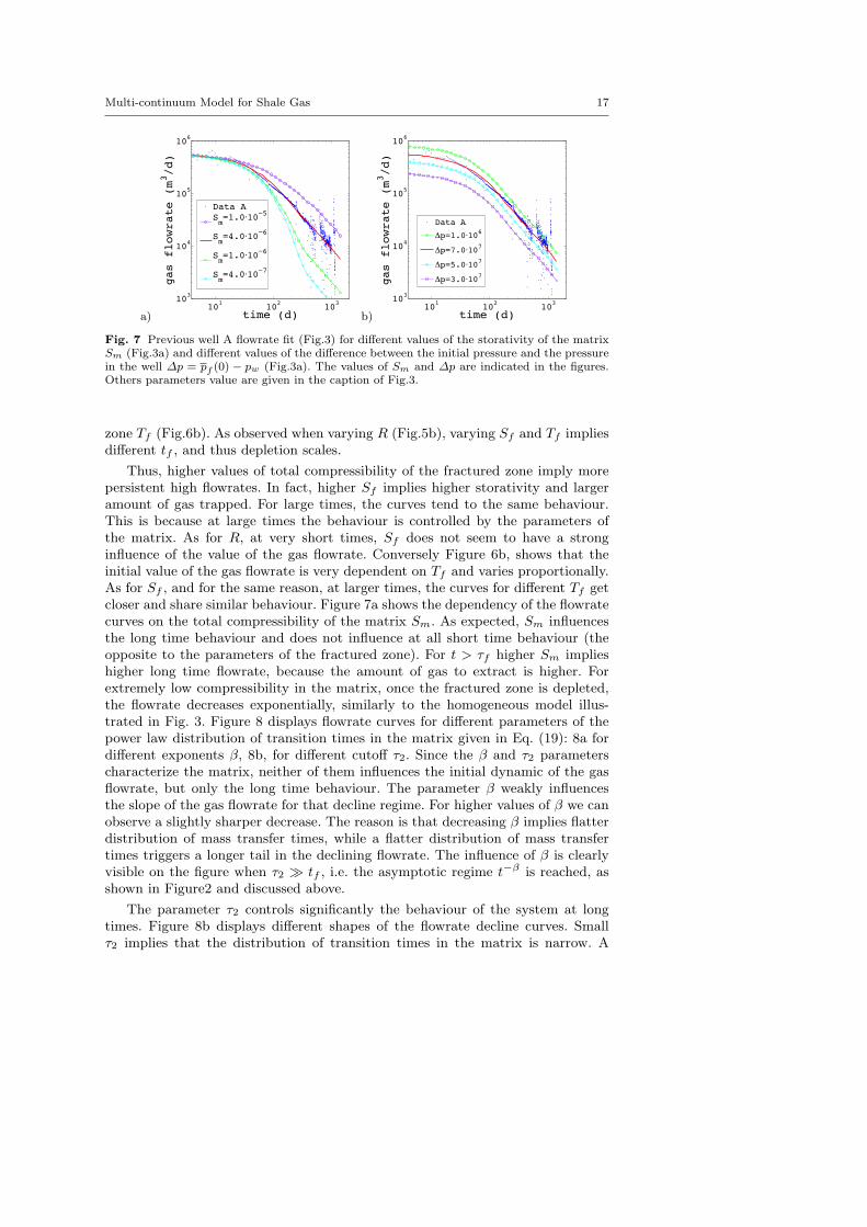
Fig. 7 Previous well A flowrate fit (Fig.3) for different values of the storativity of the matrixSm (Fig.3a) and different values of the difference between the initial pressure and the pressurein the well ∆p = pf (0) − pw (Fig.3a). The values of Sm and ∆p are indicated in the figures.Others parameters value are given in the caption of Fig.3.

zone Tf (Fig.6b). As observed when varying R (Fig.5b), varying Sf and Tf impliesdifferent tf , and thus depletion scales.

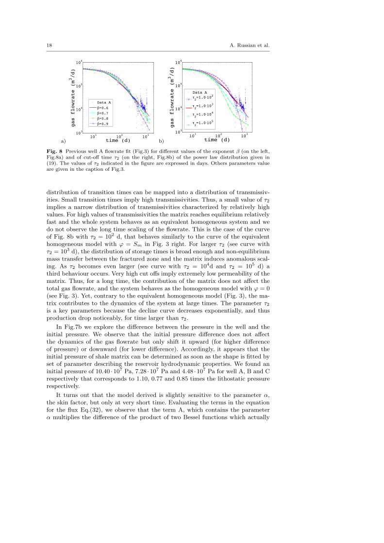
Thus, higher values of total compressibility of the fractured zone imply morepersistent high flowrates. In fact, higher Sf implies higher storativity and largeramount of gas trapped. For large times, the curves tend to the same behaviour.This is because at large times the behaviour is controlled by the parameters ofthe matrix. As for R, at very short times, Sf does not seem to have a stronginfluence of the value of the gas flowrate. Conversely Figure 6b, shows that theinitial value of the gas flowrate is very dependent on Tf and varies proportionally.As for Sf , and for the same reason, at larger times, the curves for different Tf getcloser and share similar behaviour. Figure 7a shows the dependency of the flowratecurves on the total compressibility of the matrix Sm. As expected, Sm influencesthe long time behaviour and does not influence at all short time behaviour (theopposite to the parameters of the fractured zone). For t > τf higher Sm implieshigher long time flowrate, because the amount of gas to extract is higher. Forextremely low compressibility in the matrix, once the fractured zone is depleted,the flowrate decreases exponentially, similarly to the homogeneous model illus-trated in Fig. 3. Figure 8 displays flowrate curves for different parameters of thepower law distribution of transition times in the matrix given in Eq. (19): 8a fordifferent exponents β, 8b, for different cutoff τ2. Since the β and τ2 parameterscharacterize the matrix, neither of them influences the initial dynamic of the gasflowrate, but only the long time behaviour. The parameter β weakly influencesthe slope of the gas flowrate for that decline regime. For higher values of β we canobserve a slightly sharper decrease. The reason is that decreasing β implies flatterdistribution of mass transfer times, while a flatter distribution of mass transfertimes triggers a longer tail in the declining flowrate. The influence of β is clearlyvisible on the figure when τ2 � tf , i.e. the asymptotic regime t−β is reached, asshown in Figure2 and discussed above.

The parameter τ2 controls significantly the behaviour of the system at longtimes. Figure 8b displays different shapes of the flowrate decline curves. Smallτ2 implies that the distribution of transition times in the matrix is narrow. A


a)101 102 103

103

104

105

106

time (d)

gas flowrate (m3/d)

Data A=0.6=0.7=0.8=0.9

b)10

110

210

310

3

104

105

106

time (d)

gas flowrate (m3/d)

Data A

2=1.0 102

2=1.0 103

2=1.0 104

2=1.0 105

Fig. 8 Previous well A flowrate fit (Fig.3) for different values of the exponent β (on the left,Fig.8a) and of cut-off time τ2 (on the right, Fig.8b) of the power law distribution given in(19). The values of τ2 indicated in the figure are expressed in days. Others parameters valueare given in the caption of Fig.3.

distribution of transition times can be mapped into a distribution of transmissiv-ities. Small transition times imply high transmissivities. Thus, a small value of τ2

implies a narrow distribution of transmissivities characterized by relatively highvalues. For high values of transmissivities the matrix reaches equilibrium relativelyfast and the whole system behaves as an equivalent homogeneous system and wedo not observe the long time scaling of the flowrate. This is the case of the curveof Fig. 8b with τ2 = 102 d, that behaves similarly to the curve of the equivalenthomogeneous model with ϕ = Sm in Fig. 3 right. For larger τ2 (see curve withτ2 = 103 d), the distribution of storage times is broad enough and non-equilibriummass transfer between the fractured zone and the matrix induces anomalous scal-ing. As τ2 becomes even larger (see curve with τ2 = 104d and τ2 = 105 d) athird behaviour occurs. Very high cut offs imply extremely low permeability of thematrix. Thus, for a long time, the contribution of the matrix does not affect thetotal gas flowrate, and the system behaves as the homogeneous model with ϕ = 0(see Fig. 3). Yet, contrary to the equivalent homogeneous model (Fig. 3), the ma-trix contributes to the dynamics of the system at large times. The parameter τ2

is a key parameters because the decline curve decreases exponentially, and thusproduction drop noticeably, for time larger than τ2.

In Fig.7b we explore the difference between the pressure in the well and theinitial pressure. We observe that the initial pressure difference does not affectthe dynamics of the gas flowrate but only shift it upward (for higher differenceof pressure) or downward (for lower difference). Accordingly, it appears that theinitial pressure of shale matrix can be determined as soon as the shape is fitted byset of parameter describing the reservoir hydrodynamic properties. We found aninitial pressure of 10.40 ·107 Pa, 7.28 ·107 Pa and 4.48 ·107 Pa for well A, B and Crespectively that corresponds to 1.10, 0.77 and 0.85 times the lithostatic pressurerespectively.

It turns out that the model derived is slightly sensitive to the parameter α,the skin factor, but only at very short time. Evaluating the terms in the equationfor the flux Eq.(32), we observe that the term A, which contains the parameterα multiplies the difference of the product of two Bessel functions which actually


gives very small values compared to the first term in the denominator. Physicallyspeaking this means that only at very early times, the flux is limited by the skinfactor, at larger times by the release flux from the matrix.

4 Conclusion

In this work we have derived an original analytical multi-continuum model thatcan be used for analyzing gas flowrates in shale reservoirs. We show that boththe low permeability and the intrinsic heterogeneity of the shale matrix controlthe complex transient regimes and the long asymptotic decreasing flowrate usu-ally observed during the gas production. The model describes the dynamics of thegas flowrate as the function of the standard physical parameters (compressibil-ity, transmissivity, ...) and the (simplified) geometry of the stimulated reservoir.Because of the manifest lack of information on the (mechanically altered) shalematrix and consequently the spatial distribution of its heterogeneity, we describedthe matrix diffusivity stochastically using a distribution of transition times. Thelatter is parametrized by τ2 and β, the cut off and the slope of the distribution,respectively.

The model predicts:1) an initial regime controlled by the properties of the transmissivity Tf anddiffusivity Tf/Sf of the fractures, as well as the length of the individual fractureR,2) a second transient regime, which covers the main production duration of thewell, where the flowrate is controlled by coupled effects of both the fractures andthe shale matrix properties; this regime corresponds to the refill of the fractures bythe matrix. This part of the gas production curve can display distinctly differenttrends including power law decline regimes: Q(t) ∝ (t/τ2)

−β where β ∈ (1/2; 1) isa lumped parameter describing the heterogeneity distribution in the matrix.3) For t � τ2 the gas production rate decreases exponentially: Q(t) ∝ exp(−t/τc)with τc ∼ R2(Sf + Sm)/Tf .

It is worth noticing that for β = 0.5 the presented model shows the scalingQ(t) ∝ t−1/2 for the gas flux, which is typical for a dual continuum model char-acterized by a homogeneous matrix domain such as the one considered by [8].These authors account for non-linear pressure diffusion within the matrix domain,which however does not alter the characteristic t−1/2–behavior. The model pro-posed in this paper accounts for a heterogeneous matrix domain and thus allowsfor different scaling behaviors.

To illustrate the applicability of the model we considered real data from threeproduction wells that display distinctly different gas flowrate behaviours. We showthat the model can accurately fit the different flowrate behaviours and that theparameter values obtained by the fitting procedure are in accordance with typicalones found in the shale reservoir literature.

As for all multi-parameter models, the reliability of the results increases ifone can constrain some parameters and, or, impose a restricted range of vari-ability. In our model one have six parameters which are often poorly knownR, Sf , Tf , Sm, β, τ2. Any reliable data concerning these parameters will dramat-ically reduce the uncertainties on the parameter estimation and consequently onthe predictability of this tool. For instance, a good estimation of R could be surely


obtained by micro-seismic. Likewise, a better knowledge of the fracture proper-ties from geophysical or experimental data will improve the best fitting of theshort time behavior, while (multi-scale) measurements of the matrix dispersivitywould be of great importance for long term predictions. Yet, the reliability of suchmeasurements on mechanically extracted cores may be arguable and an accurateevaluation of the actual effect of fracking on the matrix properties remains highlychallenging. Accordingly, we believe that our model may be useful for tackling thematrix properties once the other parameters, including the fracture properties, areindependently estimated.

A Derivation of the memory function

We assume that the lower cut-off scale τ1 in (19) is much smaller than the upper cut-off τ2 sothat τ1/τ2 � 1 and we approximate

Pim(τ) =1− β

τ2

„τ

τ2

«−β

Θ(τ2 − τ). (41)

Inserting (41) in (18), the memory function for a multi-continuum model with a constantretardation factor reads:

ϕ(t) = Sim1− β

τ2

„t

τ2

«−β∞Z

t/τ2

dz zβ−1g′(z), (42)

where g′(z) is defined as: g(t, τ) = 1τ

g′`

tτ

´. The local memory function g(t, τ) can be ex-

pressed as above from the definition of g(ω, τ) given in (11), we note that g(ω, τ) is precisely a

function of the product ωτ . The function g′(z) behaves as z−1/2 for z < 1 and decays exponen-tially fast for z � 1. Thus, we approximate it here by the truncated power-law distribution:g′(z) = z−1/2 exp(−z)/Γ (1/2). Inserting the previous approximation into (42) and executingthe integral for the memory function ϕκ(t) reads

ϕ(t) = Sim1− β

τ2Γ (1/2)

„t

τ2

«−β

Γ (β − 1/2, t/τ2). (43)

This function behaves as a power-law according to t−β for t � τ2 and is cut-off exponentiallyfast for t � τ2. Thus, we approximate it by the truncated power-law given in (20).

B General solution of the model

The general solution of Eq. (15) is given by a combination of modified Bessel functions of firstkind I0(·) and second kind K0(·) [36]:

〈pf (r, λ)〉 = N(λ) K0[rp

λτ ′(λ)] + M(λ) I0[rp

λτ ′(λ)] +pf (r, 0)

λ, (44)

with τ ′(λ) defined in Eq.(25). The functions N(λ) and M(λ) do not depend on the radial co-ordinate r and are determined by imposing the given boundary condition in the general solution(44). Considering no radial flux at r = R, Eq.(27), we obtain: N(λ) = M(λ) I1[r

√λτ ′]/K1[r

√λτ ′]

and by imposing Cauchy-type boundary condition at the well, Eq.(26), we obtain M(λ). Byinserting N(λ) and M(λ) in Eq.(44) and rearranging the terms we obtain Eq.(23).


C Asymptotic expansion

In order to evaluate the asymptotic behavior of the gas flux Q(t), we consider the expansionof the Bessel functions in (32) for small arguments x,

K0 (x) = − ln(x/2) + . . . (45)

I0 (x) = 1 + . . . (46)

K1 (x) =1

x+

1

2ln x . . . (47)

I1 (x) =x

2. . . , (48)

where the dots denote sub-leading contributions. Substituting these expansion into (32) weobtain:

Q∗(λ) 'πTf

“R′2 − r′2w

” hpf (0)

λ− p∗w(λ)

i1 + R′2

2ln R′

r′w+ A

2

`R′2 − r′2w

´ . (49)

Setting the pressure in the extraction well constant, i.e., pw(t) = pw = constant, which impliesp∗w(λ) = λ−1pw, and substituting r′, R′ and r′w by (24) and (29) we obtain Eq.(33).

D Nomenclature

a, bi rock and fluid compressibility [Pa−1]k permeability, [L2 ]Nf number of fracture stages [-]pw pressure in the horizontal well [M L−1 T−2]p spatially averaged pressure [M L−1 T−2]〈p〉 mean pressure averaged spatially and stochastically [M L−1 T−2]Q gas rate production [L3 T−1]r radial distance from the edge of horizontal well, [L]rw radius of horizontal well, [L]R radial extension of the fractured zone, [L]s effective compressibility [Pa−1]t time, [T]tf mean diffusion time in the fractured zone[T]tm mean diffusion time over the thickness of the matrix [T]z local spatial distance from the fractured zone [L]

α outflow constant [ L−3 T−1 M ]β exponent of truncated power law distribution , [-]µ viscosity, [M T−2]λ Laplace variable [T−1]ρi density [M L−3]τ1 lower limit truncated power law distribution [T]τ2 cut-off truncated power law distribution [T]τa activation time of the drainage matrix [T]ϕ memory function of the multi-continuum model [T−1]

Derived quantities:Ki = ki/µi permeability divided by viscosity, [L3 M−1 T]Si = zisi total effective compressibility, [m Pa−1]Ti = ziKi effective transmissivity [L4 M−1 T ]


E Acknowledges

The authors gratefully acknowledge the financial support for this project from Imperial Col-lege, London, Joint Industry Project on Well Test Analysis in Complex Fluid-Well-ReservoirSystems, funded by BG Group, BHP-Billiton, Petro SA, Schlumberger and Eon-Rurhgas. Theyare grateful to BG Group and BHP-Billinton for providing the data used in this study. M.D. acknowledges the support of the European Research Council (ERC) through the projectMHetScale (contract number 617511).

References

1. J. Arps, SPE-945228-G Trans. AIM(160), 228 (1945)2. W.J. Lee, R.E. Slide, in SPE-130102, vol. 130102 (2010), vol. 1301023. D. Ilk, A. Perego, J. Rushing, T. Blasingame, in SPE-116731, vol. 116731 (2008), vol.

1167314. A. Araya, E. Ozkan, SPE-77690 77690 (2002)5. L. Mattar, B. Gault, K. Morad, C.R. Clarkson, C.M. Freeman, SPE 119897 (2008)6. F. Medeiros, B. Kurtoglu, M. Oil, E. Ozkan, SPE Reservoir Evaluation & Engineering

110848(June), 559 (2010)7. M.J. Fetkovich, SPE, Journal of Petroleum Technology pp. 1065–1077 (1980)8. T.W. Patzek, F. Male, M. Marder, Proceedings of the National Academy of Sciences of

the United States of America 110(49), 19731 (2013). DOI 10.1073/pnas.1313380110. URLhttp://www.pubmedcentral.nih.gov/articlerender.fcgi?artid=3856843&tool=pmcentrez&rendertype=abstract

9. S. Maxwell, C. Waltman, N. Warpinski, N. Mayerhofer, M.J., Boroumand, in SPE-102801,vol. 102801 (2006), vol. 102801

10. G.I. Barenblatt, I.P. Zheltov, I.N. Kochina, PMM 24(5), 825 (1960)11. J.E. Warren, P.J. Root, The Soc. Petrol. Eng. J. 3(3), 245 (1963)12. D. Bourdet, A.C. Gringarten, in SPE Annual Technical Conference and Exhibition, 21-24

September, Dallas, Texas (Society of Petroleum Engineers, Dallas, Texas, 1980). DOI10.2118/9293-MS

13. C.R. Dykhuizen, Water Resources 21(12), 1531 (1987)14. R.R. Peters, E.A. Klavetter, Water Resources Research 24(3), 416 (1988)15. M. Bai, D. Elsworth, J.C. Roegiers, Water Resources Research 29(6), 1621 (1993)16. M.J. Gatens, W.J. Lee, H.S. Lane, A.T. Watson, D.K. Stanley, Journal of Petroleum

Technology 41(5), 519 (1989)17. A.T. Watson, M.J. Gatens, J.M. Lee, Z. Rahim, SPE Reservoir Engineering 5(3) (1990)18. K. Serra, a.C. Reynolds, R. Raghavan, a.C. Reynolds, Journal of

Petroleum Technology 35(12) (1983). DOI 10.2118/10780-PA. URLhttp://www.onepetro.org/mslib/servlet/onepetropreview?id=00010780&soc=SPE

19. E. Carlson, J. Mercer, Journal of Petroleum Technol-ogy 43(4) (1991). DOI 10.2118/19311-PA. URLhttp://www.onepetro.org/mslib/servlet/onepetropreview?id=00019311&soc=SPE

20. K.L. Kuhlman, B. Malama, J.E. Heath, Water Resour. Res. 51(2), 848 (2015). DOI DOI:10.1002/2014WR016502

21. A.H. El-Banbi, Analysis of Tight Gas Well Performance. Ph.D. thesis (1998)22. R.O. Bello, R.A. Wattenbarger, SPE, Journal of Canadian Petroleum Technology 49(12),

143229 (2010). DOI 10.2118/143229-PAContent23. I. Neuweiler, D. Erdal, M. Dentz, Vadose Zone Journal 11, 0 (2012). DOI

10.2136/vzj2011.013224. J. Tecklenburg, I. Neuweiler, M. Dentz, J. Carrera, S. Geiger, C. Abramowski, O. Silva,

Advances in Water Resources 62, 475 (2013). DOI 10.1016/j.advwatres.2013.05.012. URLhttp://dx.doi.org/10.1016/j.advwatres.2013.05.012

25. S. Geiger, M. Dentz, I. Neuweiler, SPE Journal 18(8), 670 (2013). DOI 10.2118/148130-MS. URL https://www.onepetro.org/journal-paper/SPE-148130-PA

26. J. Bear, Dynamics of fluids in porosu media, dover edn. (American Elsevier PublishingCompany, New York, 1972)

27. R. Haggerty, S.M. Gorelick, Water Resources Research 31(10), 2383 (1995)28. J. Carrera, X. Sanchez-Vila, I. Benet, A. Medina, G. Galarza, J. Guimera,

Hydrogeology Journal 6(1), 178 (1998). DOI 10.1007/s100400050143. URLhttp://www.springerlink.com/openurl.asp?genre=article&id=doi:10.1007/s100400050143


29. M. Abramowitz, I. Stegun, Handbook of Mathematical Functions with Formulas, Graphs,and Mathematical Tables (Dover Publications, New York, 1965)

30. K.J. Hollenbeck. INVLAP.M: A matlab function for numerical inversion of Laplace trans-forms by the Hoog algorithm (1998). URL http://www.isva.dtu.dk/staff/karl/invlap.htm

31. A. Cortis, B. Berkowitz, Ground Water 43(6), 947 (2005). DOI 10.1111/j.1745-6584.2005.00045.x

32. B. Berkowitz, A. Cortis, M. Dentz, H. Scher, Rev. Geophys. 44(RG2003), RG2003 (2006).DOI 10.1029/2005RG000178.1.INTRODUCTION

33. D.G. Friend, J.F. Ely, H. Ingham, J.Phys. Chem. Ref. Data 18(2), 583 (1989)34. C.E. Neuzil, Water Resources Research 30(2), 145 (1994). DOI 10.1029/93WR02930. URL

http://doi.wiley.com/10.1029/93WR0293035. W. Yu, K. Sepehrnoori, Proceedings of 2013 SPE Production and Operations Sympo-

sium 2013 (2013). DOI 10.2118/164509-MS. URL https://www.onepetro.org/conference-paper/SPE-164509-MS

36. H.S. Carslaw, J.C. Jaeger, Conduction of Heat in Solids, vol. 36 (Oxford University Press,Oxford, 1947). DOI 10.2307/3610347

Multi-Continuum Approach to Modeling Shale Gas...

Documents

Transcript of Multi-Continuum Approach to Modeling Shale Gas...