Master Thesis

Multi-Asset Factor Investing

Simona Chocheva

357026

Supervised by Dr. R. Xing

Erasmus School of Economics

Erasmus University

September 2017

2

Abstract

In this paper, the performance of three factor investing strategies for U.S. market is being explored.

According to financial studies, low-volatility-, value- and momentum strategies have proven to

generate systematic yield across various asset classes. However, the literature on this topic is

inconclusive about the effect of each factor investment strategy on a multi-asset portfolio. Unlike

previous studies, this paper focuses on examining the impact of factors on a multi-asset portfolio,

consisting of equities, corporate investment bonds, high-yield bonds, commodities and REITs. This

study builds on the current financial literature by using more recent dataset 1990-2015, along with

analyzing factor strategies both per individual asset classes, as well as combined in a multi-asset

portfolio. The results indicate that low-volatility, value and momentum strategies can be

beneficially exploited for both the multi-asset portfolio and individual asset classes. The multi-

asset portfolio has generated the highest alpha spread and Sharpe ratio when exploiting low-

volatility strategy. For value and momentum strategies, REITs have outperformed the Sharpe ratio

of the multi-asset portfolio. Additionally, robustness checks proved that the financial crises had an

impact on the yields across individual assets and on the multi-asset portfolio.

Keywords: factor investing, multi-asset portfolio, equities, bonds, commodities, REITs

3

Table of Contents

Section I: Introduction ................................................................................................................... 4

Section II: Literature review ......................................................................................................... 6

i. Low-volatility ................................................................................................................... 8

ii. Value ................................................................................................................................. 9

iii. Momentum ...................................................................................................................... 10

Section III: Data and Research Questions ................................................................................. 12

i. Data ................................................................................................................................. 12

ii. Research Questions ......................................................................................................... 13

Section IV: Methodology ............................................................................................................. 13

Section V: Empirical Results ....................................................................................................... 17

i. The Low-volatility anomaly ........................................................................................... 17

ii. Value effect..................................................................................................................... 20

iii. The Momentum impact .................................................................................................. 22

Section VI: Robustness checks .................................................................................................... 25

Section VII: Concluding Remarks .............................................................................................. 26

Bibliography ................................................................................................................................. 29

Appendix ....................................................................................................................................... 33

4

Section I: Introduction

Nowadays, an increasing number of investors are hunting for systematic yield. In the 1970s

researchers questioned the conventions of the CAPM model that assumes rational markets and

investors, and forecasts positive linear relationship between risk and return. One of the first who

investigated stock` yields and established that the relationship between risk and return is not linear

are Treynor, 1962, Sharpe, 1964, Black, 1972. Contrary to the fundamental CAPM theory market

risk does not fully explain all stock performance, but other factors do so. Fama and French, 1996,

acknowledged the presence of asset pricing anomalies and conclude that small- and value stocks

produce higher returns.

Present empirical work has proved that investing based on particular features of assets, also referred

to as ‘factor investing’, may lead to greater risk- adjusted returns (Asness, Markowitz and Pedersen,

2013). A fascinating market phenomenon is the value effect which represents the relation between

an asset’s return and the ratio of its book value relative to its current market value. The overview

of factor investing could very well continue with Jegadeesh and Titman who verified that buying

stocks that have performed well in the past and selling stocks that have performed poorly in the

past could lead to excess return. This phenomenon is now accredited as the momentum effect.

Momentum investing is ‘a lively game of hot potato - buying rapidly appreciating stocks, holding

them for a relatively short period, and selling them before their price trends reverse direction.’

(Larson, 2013). Asness, Moskowitz and Pedersen, 2013, establish that value and momentum effect

occur across globe and asset classes. Blitz and Van Vliet (2007) further contribute to the factor

investing literature and provide empirical evidence that stocks with low volatility produce high

risk-adjusted returns. This effect is now known as the volatility effect and it has been proven to be

present across the U.S., European and Japanese markets. Besides, Blitz and Van Vliet also proved

that size and value effect are not the reason why the volatility effect occurs. They argue that

investors should treat low risk stocks as a distinct asset class in the asset allocation phase, in order

to exploit this anomaly in practice.

Based on the aforementioned academic studies, it can be summarized that by allocating to value,

momentum and low volatility factors, systematic excess return can be reaped. Attracted from the

5

upside potential from factor investing, experts started exploiting these market anomalies by

transforming them into investment strategies, which have led to the evolution of factor investing.

However, there is a lack of consent on what factor investing really is and what distinguishes it from

the traditional quantitative investment methods. Factor investing is a systematic approach to

investing strategically in specific parts of the financial markets which generate better returns over

longer periods than those in other sectors. According to the financial literature, factor premiums

have been proven to be robust over time. Such premiums have been also observed in the multi-

asset space. Therefore, factor investing could be exploited not only for stocks but could potentially

be taken advantage of in other asset classes.

Now, it is well known that with stock pitching an investor faces the risk of under diversification,

hence making him/her exposed to a substantial idiosyncratic risk. The literature on market

anomalies mainly examines factors individually. Inspired by these studies, this paper contributes

to and extends the existing factor investing literature in several ways. First, it fills the literature gap

by comparing the performance of the different factors on multi-asset portfolio, as this offers

diversification benefits for investors. Second, it produces robust empirical estimates of the alpha

spread for momentum, total volatility and value. Lastly, this study utilizes a portfolio based

regression approach, inspired by Fama and French (1996), to examine the excess return that can

potentially be achieved and analyzes relatively recent data (1990-2015) across the U.S. market.

The main goal of this research is to analyze whether an investment strategy based on the value,

momentum and low-volatility anomaly is worthwhile. Consequently, this paper will aim to prove

a consistent excess return premium that can be achieved if the above-mentioned market anomalies

are put into practice.

The remainder of this paper is organized as it follows: Section II documents relevant literature on

the risk-return relationship. Section III elaborates on the data collection procedure and formulates

the research questions, while section IV describes the methodology. Next, Section V delivers the

results and the corresponding implications. Additionally, Section VI addresses robustness checks.

Finally, Section VII is centered on concluding remarks.

6

Section II: Literature review

Researchers have found that market anomalies (referred to as factors in the above section I.) are

responsible for a large portion of the market outperformance. Consequently, factor investing is

attracting higher attention as an effective investment model and a growing number of institutions

have shifted their attention from a traditional asset allocation approach towards a factor allocation

approach. As a result, diversification occurs by allocating to different factor premiums that have

superior risk/return profiles than market-capitalization weighted indices. Some of the most

widespread factors in this respect are value, momentum and low-volatility. Therefore, it is

important to analyze the impact of each of these factors on a multi-asset portfolio as this might

offer not only diversification benefits to investors, but also greater yield and Sharpe ratio.

As mentioned above, important market anomalies that are exploited for stocks are the value

premium (Fama and French, 1992), the size premium (Banz,1981), the momentum premium

(Jagadeesh and Titman, 1993) and the low-volatility premium (Blitz and van Vliet,2007).

However, factor premiums have a larger presence also elsewhere rather than just within equities.

They can be found in other asset classes such as bonds and commodities (Asness, Moskowitz and

Pedersen, 2009), while the low volatility effect could be taken advantage of in credits (Houweling

et al.,2005). When taking into consideration all factor premia, momentum is considered one of the

most attractive and is in most cases part of every equity` factor investment strategy, mainly because

of its low correlation with factors like low volatility and the fact that it can have a negative

correlation with value. Consequently, investors tend to hedge their portfolios against reversal risk

(‘winner’ stocks to become ‘loser’ stocks) that might occur with momentum investing strategy and

minimize the related transaction costs, by combining momentum with other factors. When it comes

to corporate fixed income market- size, low-risk, value and momentum factors have economically

meaningful and statistically significant risk-adjusted returns. Besides, Houweling, 2014, shows that

in a multi-asset framework, allocating to corporate bond factors has generated returns beyond the

ones from allocating to equity factors.

Before it is proceeded to the in-depth literature review of the above-mentioned factors, it is

7

important to discuss the fundamental Capital Asset Pricing Model, which serves as a stepping stone

in the finance literature. Grounded on the portfolio theory from Markowitz (1959), CAPM is a

theoretical model that assumes that the expected return on a stock is only dependent on its

systematic risk (Sharpe, 1964, Lintner, 1965). However, the theory of CAPM and what happens in

reality are in big contrast. The following paragraphs will elaborate more on the CAPM model,

followed by an overview of the literature on factors.

Sharpe (1964) `s and Lintner (1965) `s CAPM method tries to explain how to evaluate risk, as well

as its connection to the expected asset`s return. Berk and DeMarzo, 2014, highlight the three main

assumptions of the CAPM model, to evaluate its effectiveness. First, all investors have identical

outlooks concerning the expected return of the assets, their correlations and volatilities. Second,

investors can borrow and lend at the risk-free interest rate, in addition to trade all assets at market

price. The third postulation is that investors keep only such portfolios that generate the greatest

expected yield for a given level of risk. However, Fama and French, 2004 prove that these

assumptions of the CAPM are not representative for the whole market. As explained in the

introduction section, Black, 1972, Lucas, 1978, Fama and French, 1992, Barberis et al., 2015

establish that market anomalies are present and are founded based on CAPM. For instance, Russel

and Thaler, 1985, De Long, 1990, find a mismatch between reality and CAPM assumptions. When

studying investors behavior, the authors find that investors are not entirely rational.

Furthermore, De Bondt and Thaler, 1994, presents the concept of irrationality among investors

(Shleifer, 2000) and how more sophisticated investors can benefit from exploiting the market

anomalies that might occur because of this behavioral bias. For instance, Daniel, Hirshleifer and

Subrahmanyam, 1998, Barberis, Shleifer and Vishny, 1998, show that investors can either

overreact or underreact (Hong, Stein, 1999, Chan, Jegadeesh and Lakonishok, 2006) to unexpected

events or news, which can cause momentum outcome. From the studies of Daniel, Hirshleifer and

Subrahmanyam, 1998, Barberis, Shleifer and Vishny, 1998, Hong and Stein, 1999, it can be

summarized that the overreaction or underreaction can be mainly caused by lack of analyzing

capabilities, overconfidence, self-attribution, conservatism bias, or loss aversion. Value and

momentum anomalies could also occur due to flows between the investment capitals (Vayanos and

Woolley, 2012). Additionally, momentum anomaly could also occur because of collective

8

managers’ behavior, also referred to as ‘herding’ behavior (Dasgupta, Prat, and Verardo, 2011) as

managers that are in a group can take collective decisions without a specific direction. Hence, this

can cause an investment biased decision.

On the other hand, the rationality of CAPM is also investigated by Jagannathan and Wang, 1996

who prove as well that the model does not measure entirely the risk and does not cover the complete

relationship between risk and expected return. Other financial studies such as Faff, 2004, also prove

that the three-factor model explains better the risk-return relationship than the traditional CAPM

model (Gaunt, 2004). Eraslan, 2013, states that the model that builds on CAPM, namely the Fama

and French three-factor model, captures the CAPM inefficiencies by incorporating factors in their

methodology.

i. Low-Volatility

There is a broad arsenal of studies that has analyzed the low-volatility anomaly and has shown that

contrary to CAPM methodology, excess return can be achieved. Research on this anomaly can very

well start with Falkenstein, 1994, who found out that the relationship between expected asset`s

return and risk has proven to be flat, or even negative, which means that CAPM expectations do

not hold. Later, Ang et al., 2006, conclude that higher risk is not necessary compensated with higher

return. In the same period, Ang, Hodrick, Ying, and Zhang, 2006, explain that this means that low-

risk stock investments should outperform high-risk stock investments. Based on the observations,

recent empirical research focused on analyzing whether low-risk stocks indeed outperform the

high-risk stocks. Baker and Haugen, 2012, examined the length of this anomaly, and the yield

differences it generates among various industries and concluded that is robust over time. Going

into more details, Baker, Bradley and Wurgler, 2011 prove that the anomaly holds even if different

risk interpretations are considered, namely low beta, or volatility (as a low volatility anomaly) as a

substitute for risk.

Low-volatility anomaly could be explained through both rational and behavioral theories. Some of

the rational theories include shorting constraints and leverage constraints. Institutional investors,

for example, are constrained in the amount of leverage they can take on and this explains the low

9

yields on the high-risk assets (Frazzini and Pedersen, 2014). Besides, investors could also face

shorting constraints, hence, if they would like to short on high-volatile asset and long on low-

volatility ones, this might not be allowed. In case that there are no shorting constraints and all

investors are to behave rationally and trade on the low-volatility anomaly, the phenomenon is likely

to disappear. However, this cannot happen in practice as investors do not behave in the same way.

On the other hand, when we look at the behavioral explanations of this anomaly, the concept of

lottery disposition (Kahneman and Tversky, 1979) might apply. The authors demonstrate that when

people should make a choice between a low chance of a significant gain and a high chance of small

loss, they will rather go for the riskier option. Kumar, 2009, Barberis and Huang, 2008, Bali, Cakici

and Whitelaw, 2011, also confirm the theory that investors are likely to take on the hazard of

investing in high volatility stocks as they will be exposed to a chance of earning excess return.

Furthermore, Baker, Bradley and Wurgler, 2011, explain that overconfidence bias might cause

investors to stick to their initial strategy, because they feel overconfident in their analysis.

Additionally, Baker, Bradley, and Wurgler, 2011, state that irrational investors tend to evade low

risk stocks and tend to pay more for hazardous stocks.

To test whether low-volatility strategy could generate excess return, researchers deploy relatively

similar statistical methods. Initially, stocks are sorted based on volatility levels and then allocated

to equally weighted portfolios. Every month each portfolio is being rebalanced. CAPM` and Fama

and French three-factor model` alphas are attained within each quintile or decile of the equally

weighted portfolios.

ii. Value

Value effect is present across most asset classes, thus is one of the most implemented factor

investing strategies (Asness, et all, 2013). Basu (1977), Rosenberg, Reid, and Lanstein (1984) show

that strategies based on book-to-market ratios have produced excess returns over a long-term period

(De Bondt and Thaler (1985, 1987)). In line with Merton (1973), Fama and French, 1992, also

demonstrate that the excess return occurs as a compensation for risk. On the contrary, Lakonishok,

Shleifer, and Vishny,1994, argue that there is little evidence that high book-to-market ratio and

high cash-flow-to-price stocks are riskier based on traditional concepts of systematic risk. For

10

diverse reasons, Lakonishok, Shleifer, and Vishny, 1994, conclude that value stocks have been

underpriced relative to their risk and return. Daniel and Titman, 1996, also state that value stocks

deliver excess return because it takes time for the markets to realize that earnings growth rates for

value stocks are higher than initially expected and opposite to attractive stocks. In addition,

LaPorta, Lakonishok, Shleifer, and Vishny. 1997, show that significant portion of the return

difference between value and attractive stocks is because of earnings surprises that are

systematically more positive for value. Moreover, Piotroski, Joseph, 2000 test that when using a

simple check based on historical financial performance, investors can indeed earn abnormal return

by creating strong value portfolio. Based on the financial literature it can be summarized that

empirical evidence proves that the value effect is significantly strong, no matter the reason why

strategy works in practice (Asness, 1997).

iii. Momentum

The momentum anomaly is one of the most widely studied phenomenon in capital markets. Among

the first studies of the momentum effect was conducted by Levy (1967), who found that significant

abnormal returns are generated by holding stocks with higher than average prices over the recent

past period. Later, Jegadeesh and Titman (1993) also established that past winners in the U.S.

capital markets outperform previous losers. The research of Jegadeesh and Titman (1993) ranked

each month the returns of companies over the past 6 months. Decile portfolios were formed based

on these rankings, where the top decile is called ‘winners’ and bottom decile is called ‘losers’.

Jegadeesh and Titman (1993) documented that above 10% average excess return per year could be

achieved by using 6 months of past return. Going more in-depth, Asness (1997) concluded that

winners become losers and losers become winners over the long-term. Pursuing the methodology

by Jagadeesh and Titman (1993), Rouwenhorst (1998) found similar outcome for the European

market. However, researchers have established that for the last hundred years there have been

several periods during which the returns from winning stocks have totally crashed. Momentum

premium could drop significantly, impacting severely the profits of investors (Cooper, Guitierrez

and Hameed (2004). Other studies such as Sun and Stivers (2010) show as well that momentum is

procyclical, especially in periods such as the recent financial crises. Based on the aforementioned

risks that momentum strategy carries, risk-averse investors might dislike momentum investing. On

11

the other hand, hazardous investors would like to take on this risk and through a well-diversified

factor portfolio to manage to hedge the possibility of a reversal risk. Barroso and Santa Clara, 2013,

also show that in hand with its extraordinary performance, momentum might also sporadically

crash (Daniel and Moskowitz, 2014). Therefore, it is necessary momentum risks to be hedged by

incorporating value effect in investors’ portfolios (as explained above), due to the negative

relationship between these two factors.

Referring to the above paragraph that mentions factor cyclicality, it is important to describe what

it means in practice. Factor indices have demonstrated that ‘excess risk adjusted returns over long

time periods’ have exhibited ‘significant cyclicality which sometimes includes periods of

underperformance’ (Bender, 2013). Exhibit 1 below shows that some of the factor indices exhibited

2-3 years of underperformance for the period 1988-2013. Hence, for a factor investing strategy to

work, an investor should consider a long-term strategy. Therefore, only a long-term investor could

be able to exploit this investment approach as investors with shorter horizons would not be able to

benefit from the full cycle required for factor investing to generate excess return.

Exhibit 1: All systematic factors are cyclical (cumulative returns, June 1988 to June 2013)

Source: https://www.msci.com/documents/1296102/1336482/Deploying_Multi_Factor_Index_Allocations_in_Institutional_Portfolios.pdf/857d431b-d289-47ac-a644-b2ed70cbfd59

12

Section III: Data and Research Questions

i. Data

Equities

The examined period in the study covers the period January 1990 to December 2015. The daily

adjusted closing prices expressed in U.S. dollars of equities of the United States are gathered from

Thomson Reuters DataStream. SandP500 index is be used and inn the analysis monthly stock prices

are utilized.

The risk-free rate and the factors - market, size, value, and momentum - are provided by the

Kenneth French data library. In the financial literature, this is a common proxy for the risk-free

rate (Bollerslev, Engle and Wooldridge, 1988). Consequently, for the risk -free rate the one- month

U.S. Treasury bill (T-bill) rate is applied.

Bonds

For the period January 1990 to December 2015, survivorship-bias free data of the Barclays U.S.

Corporate Investment Grade index and the Barclays U.S. Corporate High Yield index are collected

from DataStream. Barclays provide various full characteristics of each bond in each month

(Houweling,2014). To estimate the factor portfolios, the excess return of a corporate bond versus

duration-matched Treasuries is used. Barclays offers also these excess returns. (Houweling, 2014).

Commodities

Commodity prices and returns are obtained from data stream covering the U.S. market. Examined

period covers also the beginning of 1990 to the end of 2015. Going into more details, SandP GSCI

Commodity total return (OFCL) index is downloaded. For consistency with the data gathering

process of the variables, only monthly data is collected.

13

REITs

REIT`s data is collected from the Center for Research in Security Prices (CRSP)/ Ziman Real

Estate Database. The used data frequency is monthly and the chosen period is as well 1990 to 2015.

ii. Research Questions

This paper will aim to investigate the following research question:

Which factor investing strategy generates the greatest yield on a multi-asset portfolio?

Research Sub-Questions:

• Which factor investing strategy will generate the highest yield per asset class?

• Which factor investing strategy will generate the biggest yield for the multi-asset

portfolio?

• Is the multi asset portfolio`s Sharpe ratio greater than the one of per asset class?

The above questions give an indication of what answers could be found in the results section of

this study.

Section IV: Methodology

Low-volatility

The Center for Research in Security Prices (CRSP), the monthly returns from 1990 to 2015 for all

stocks traded on NYSE, NASDAQ and AMEX are taken. Then, the monthly volatility is calculated

in the same way as in Blitz and Van Vliet (2007). Excess returns are calculated by deducting the

risk-free rate, measured by the short-term interest rate, taken from the Kenneth French database.

14

All portfolios are updated on a monthly basis and at the end of each month, stocks are being ranked

on the past 6-month volatility of returns, following AN et al., (2014). Subsequently, equally-

weighted quintile portfolios are constructed based on these rankings. Stocks with the lowest

(highest) volatility are assigned to quintile one (five). Afterwards, the (excess) mean return is

calculated for each portfolio. These portfolios have a holding period of 1 month, after which the

portfolio is rebalanced. The obtained time-series of the five portfolios will be utilized in the

regression analysis to estimate the alpha of each portfolio. The CAPM and the Fama and French 3

factor model are implemented as a benchmark.

Furthermore, a slightly different approach is undertaken for the multi-asset portfolio construction.

The asset classes are first ranked according to their individual volatility periods and only then the

multi-asset portfolio is formed based on the per asset` s volatility rankings. Additionally, different

volatility periods per asset class will be first analyzed so that it can be explored on which volatility

window each asset generates the highest Sharpe ratio. Based on this analysis, the multi asset

portfolio will be constructed by taking the most efficient combinations of volatility periods per

asset class.

Value

As in most financial literature, equities are being sorted on their book to market value, following

the approach of Fama and French (1992) and Lakonishok, Shleifer, and Vishny (1994). For all

other asset classes, the methodology of Asness, Moskowitz and Pedersen (2013) will be followed.

As ‘uniformity across asset classes is difficult to be achieved, a rather simple and consistent

measures of value will be used’. (Asness, et all, 2013). For bonds, the 5-year change in the yields

of investment-grade and high-yield bonds will be computed. The result will be like the negative of

the past 5-year return on these bonds. (Asness, et all, 2013). For commodities, value is estimated

as the log of the spot price 5 years ago, divided by the most recent spot price. (Asness, et all, 2013).

Consequently, the negative of the spot return over the last 5 years is utilized (Asness et all, 2013).

Unfortunately, the paper of Asness, 2013, does not consider REITs, therefore this study will build

on the paper ‘Value and Momentum everywhere’ (Asness, et all, 2009) by also investigating value

effect on REITs. This will also be tested by replicating the aforementioned methodology.

15

Consequently, according to the asset`s value, ranks will be assigned and quintile portfolios will be

formed (by following the method of the low-volatility investment strategy). Thereafter, excess

returns are calculated with the purpose of estimating the per asset class’s pricing error of each

regression.

Momentum

To measure momentum, the simplest and most commonly used measures are utilized. This paper`s

goal is to maintain a simple and fairly uniform approach that is consistent across asset classes’

(Asness, Moskowitz, Pedersen, 2013). This study implements a simple portfolio-based regression

methodology to analyze the momentum effect. To do so, momentum portfolios are formed for

equities, investment-grade-, high-yield- bonds, commodities and REITs. Going into more details,

strategy based on cumulative returns of 12 months and strategy based on cumulative returns of 6

months will be deployed with the purpose of testing which one generates the highest yield per asset

class. At the end of each month, the asset classes are being ranked on their cumulative returns,

following Jegadeesh and Titman, 1993. Subsequently, equal-weighted quintile portfolios are

created based on these rankings. Stocks, bonds, commodities and REITs with the highest (lowest)

cumulative returns are assigned to the top (bottom) quintile. Subsequently, the (excess) mean return

is calculated for each portfolio. Following the approach of low-volatility and value strategies, the

portfolios also have a holding period of 1 month, thereafter being rebalanced. Most of the analysis

are focused on the zero-investment portfolio that is calculated by taking the difference in returns

per month between quintile 5 and quintile 1. The obtained time-series will be utilized in the

regression analysis to estimate the pricing error of each portfolio against the two benchmark models

mentioned above, namely the CAPM and Fama and French 3 Factor model.

Construction of the Multi-Asset Portfolio

Before creating the multi-asset portfolio, regressions will be first run per asset class and per factor.

Thereafter, a combined portfolio consisting of equities, bonds, commodities and REITs is

constructed and the regressions are applied per factor on the multi-asset portfolio. Therefore, it is

important to explain the formation of the portfolio. The return of the multi-asset portfolio is

16

computed by utilizing the bellow formula:

E(R) = w1R1 + w2R2 + ...+ wnRn

where ‘E(R)’ is the expected return of the multi-asset portfolio, ‘w’ indicates weight per asset class

and ‘R’ indicates the return of an asset. Hence, the combined portfolio consists of 70% return on

equities, 10% return on combined bond portfolio return (50% weight in high yield bonds and 50%

weight in investment grade bonds), 10% return on commodities and the remaining 10% return on

REITs. The below formula shows in detail the weights per asset class for the multi asset (MA)

portfolio:

MA portfolio return = 70% *Re + 10%* Rb + 10%*Rc + 10%*Rr

where Re stands for return on equities, Rb stands for total bonds portfolio return, consisting of 50%

investment grade bonds and 50% high-yield bonds. Rc represents return on commodities, while Rr

is return on REITs. After the multi-asset portfolio return is computed, rankings are assigned as per

the above-mentioned methods. For momentum, two versions of cumulative returns of the portfolio

are being tested (cumulative returns 6- and 12 months), to check for different scenarios of when

the multi-asset portfolio generates higher return and substantial alpha spread. Subsequently,

equally-weighted quintile multi-asset portfolios are created based on these rankings. Multi-asset

portfolios with the lowest (highest) rank are allocated to quintile one (five). The rank depends on

which factor investing strategy takes place. As discussed in the above paragraphs, it is either sorted

on volatility periods for low-volatility strategy, value for value strategy or cumulative returns when

it comes to momentum. Afterwards, the (excess) mean return is calculated for each portfolio.

Alpha-spreads are computed after the regressions on CAPM and 3-factor Fama and French model

are performed. Here, as explained in the low-volatility methodology, it is useful to mention again

that for the low-volatility strategy, before the multi-asset portfolio is constructed, volatility periods

per asset class are first defined and ranked, and only thereafter the multi-asset portfolio is formed.

17

Section V: Empirical Results

As outlined in the methodology part of this paper, to test for the factor strategies across different

asset classes, cross-sectional regressions are run based on CAPM and Fama and French 3 factor

models. For each factor investing strategy, regressions are first run per asset class, namely equities,

investment grade bonds, high- yield bonds, REITs and commodities. The second step involves

constructing a multi-asset portfolio of these asset classes and analyze the effect of each anomaly

on the whole portfolio. The results below are presented in subsections that primarily indicate the

factor investing strategy and next the asset class. Here, it is important to highlight that for the all

analyzed investment strategies, the multi-asset portfolio consists of the following weights: 70%

equities, 10% bonds, 10% commodities and 10% REITs.

i. The low volatility anomaly

Cross-sectional regressions are first run based on CAPM and second on Fama and French 3 factor

models, with the aim of testing the low-volatility anomaly across different asset classes. As

outlined in the above section, individual asset classes are first ranked according to their volatility

periods and only then the multi-asset portfolio is constructed.

Equities

Table 2 presents factor loadings of the CAPM and Fama and French 3 factor models that are

regressed on quintiles sorted on the 6-month and 12- month return volatility of equities. Jensen’s

alpha across the portfolios show a significant positive effect on the excess return which indicates

that low volatility stocks generate excess return. In line with the empirical evidence, the alphas of

the portfolios increase from the first to the fifth quintile portfolio. The same observation has been

found when re-testing for the low volatility anomaly with respect to the CAPM. Furthermore, it is

important to look at the alpha spread which is the spread between the alphas of quintile 5 (P5) and

quintile 1 portfolios (P1). When analyzing the effect per equally weighted portfolios, it can be

summarized that P1 shows a significant lower alpha relative to the one of P5, which indicates

positive alpha spread and that the higher the volatility of stocks, the worst the performance on the

18

excess return, which is inconsistent with the CAPM theory, but coherent with previous research

(Blitz and Van Vliet, 2007, Baker, Bradley and Wurgler, 2011). The results on SMB and HML for

equities indicate that the value premium, and the size premium have a positive, however,

insignificant impact on the alpha spread. An interesting observation is that when equities are sorted

on 12 months volatility period, the alpha spread seems to increase, hence the bigger the volatility

period, the better performing the low-volatility strategy. Finally, Sharpe ratio of equities sorted on

6 months volatility is 0.023 and it is slightly lower than the Sharpe ratio of equities sorted on 12

months volatility (0.027) (table 11). Hence, it can be concluded that the higher the volatility

window, the higher the excess return generated from the low-volatility strategy and the higher the

Sharpe ratio.

Investment grade bonds

Unlike any other studies on this topic, low volatility anomaly has not been explored on the fixed

income market. Low-risk strategy has indeed showed that work on this asset class. However, this

paper tries to fill the literature gap and test whether low-volatility anomaly can generate excess

return. From table 2 it can also be concluded that investment grade bonds also generate positive

excess return. The results hold for both CAPM and Fama and French 3 Factor model. However,

the insignificant SMB and HML factors prove that the size premium as well as the value premium

do not contribute to a positive effect on the excess return. Hence, size and value effect do not seem

to work for this asset class. When analyzing investment grade bonds, factor loadings of the Fama

and French 3 factor model are as well regressed on quintile portfolios but this time this asset class

is analyzed by sorting it on the 12-months and 18-months return volatility. Table 2 indicates that

higher alpha spread is achieved for investment bonds sorted on 18 months. The same results have

been obtained when examining for the low volatility anomaly with respect to the CAPM. Sharpe

ratio for investment bonds sorted on 18 months is higher than for these sorted on 12 months (table

11), however, equities generated higher Sharpe ratio than this asset class.

High-yield bonds

Following the identical abovementioned approach, the effect of low-volatility investment strategy

on high-yield bonds lead to the same conclusions as for the investment grade bonds. Table 2

outlines the CAPM results as well as the Fama and French 3 factor model. Identically to the

investment grade bonds SMB and HML proved to be insignificant. In line with investment grade

19

bonds, high-yield bonds sorted on 18 months generate higher alpha spread and higher Sharpe ratio

(table 2 and 11 respectively). Consequently, based on results for investment grade bonds and high-

yield bonds it can be summarized that this anomaly could exploited to deliver positive excess return

for this asset class.

Commodities

Moving to commodities, factor loadings of the Fama and French 3 factor model are as well

regressed on quintiles, however, for this asset class different volatility windows are applied. At

first the effect of quintiles sorted on the 6-month return volatility of commodities turned out to be

insignificant. To prove that this strategy works for commodities as well as for equities, bigger

volatility period is used. The outcome was retested for portfolios sorted on 12-, 18-, 24-, 36- and

48- months’ volatility period. Nevertheless, the results for 48-months volatility window turned out

to work best and deliver the highest and significant positive alpha spread as well as Sharpe ratio

(table 2 and 11 respectively). In line with the studies SMB and HML are insignificant for this asset

class.

REITs

For real-estate the factor loadings are also regressed on equal- weighted portfolios following the

approach as for commodities. Table 2 shows the alpha spread for REITs sorted on 48 months

volatility, however this turned out to be insignificant. Furthermore, Sharpe ratio for REIT is with

negative coefficient (table 11). As a result, it can be summarized that low-volatility strategy does

not work for this asset class.

Multi-asset portfolio

It is noteworthy to explain that in the multi-asset portfolio, equities are being sorted on 12 months

volatility period, investment grade bonds on 18 months, high-yield bonds on 18 months,

commodities on 48 months and REITs on 48 months volatility windows. The multi-asset portfolio

is built by taking the different volatility periods per asset class, as each asset class is sensitive to

generate highest excess return for different volatility periods. Additionally, it is worth saying that

other versions of volatility periods for the multi-asset portfolio were analyzed, however, the above

mentioned tested volatility periods generated the highest excess return. Therefore, in the appendix

only this unique version of the multi-asset portfolio is reported.

20

Table 2 and 11 also deliver the results for the multi-asset portfolio. SMB and HML are not

significant as for the other asset classes. As it can be comprehended from table 2, positive and

significant alpha spread with a coefficient of 0.387% means that low-volatility anomaly can be

exploited for the multi-asset portfolio to deliver the highest excess return when compared to the

individual asset classes. Also, table 11 proves that the multi-asset portfolio has generated the

highest Sharpe ratio in comparison to the individual asset classes.

To summarize, referring to tables 2 and 11, the multi-asset portfolio generated the highest alpha

spread (0.387) and the highest Sharpe ratio (0.029) when in comparison to individual asset classes.

Equities sorted on 12 months and high- yield bonds sorted on 18 months volatility have the next

highest alpha spreads and Sharpe ratios. Investment bonds and commodities perform worse on this

investment strategy relative to the other assets by showing lower alpha spreads and Sharpe ratios.

On the other hand, the low-volatility anomaly does not seem to work for REITs.

ii. Value effect

Equities

When constructing value factor for equities, a traditional sorting on the book-to-market ratio is

applied. Consistent with the literature table 5 shows significant positive excess return when

analyzed with Fama and French 3 factor model. Alpha spread (P5-P1) is also positive in respect to

CAPM. Table 12 presents the Sharpe ratio from investing in this strategy (0.013) which is one of

the highest in comparison to the other individual asset classes. Investing in value contributed to

significant mispricing, therefore it can be exploited to generate substantial excess return.

For all other asset types than equities, the measures of value, attaining uniformity is more difficult

because not all asset classes have a measure of book value. Therefore, the approach from Asness,

et al., 2009, is used.

Investment grade bonds

Following the methodology for the other asset classes outlined in the methodology part of the paper

by Asness, et all, 2009, value impact on investment grade bonds is tested. Undesirably, table 5

21

shows that the generated alpha spread coefficient in investment bonds is insignificant. Besides,

table 12 shows the lowest Sharpe ratio was achieved for this asset class. As a result, investing in

value investment strategy for investment grade bonds is not beneficial. This outcome is in contrast

with Houweling,2014. Perhaps a better approach to estimating value in investment grade bonds

will support the outcome of Houweling, 2014.

High yield bonds

Contrary to the result of investment grade bonds, high-yield bonds have proven to generate positve

significant alpha spread. When compared to equities, the alpha spread of high-yield bonds is higher.

In addition, the Sharpe ratio (table 12) is also higher than the one of equities. Consequently, it can

be summarized that value effect generates excess return when investing in high yield bonds in line

with Houweling, 2014.

Commodities

As outlined in the methodology for commodities and real estate ‘value is defined as the log of the

spot price 5 years ago, divided by the most recent spot price, which is essentially the negative of

the spot return over the last 5 years’ (Asness, et all, 2009). These long-term past return measures

of value are motivated by DeBondt and Thaler (1985) who use similar measures for individual

stocks to identify “cheap” and “expensive” firms. Table 5 gives the results of testing value effect

on commodities and shows that the alpha spread is insignificant . Furthermore, table 12 shows

relatively low Sharpe ratio of 0.006, hence value effect cannot be exploited for this asset class.

REITs

As explained in the above paragraph, reit follows the same methodology to construct the value

factor as for commodities. Table 5 proves that value could be exploited for real-estate as the alpha

spread is positive and significant. Also the Sharpe ratio for REIT is the highest in comparison to

all individual asset classes and the multi-asset portfolio. This outcome is more than sufficient to

conclude that a significant contribution of higher excess return of REITs is present due to exploiting

the value factor.

22

Multi-asset portfolio

Finally, multi-asset portfolio that consists of the 4 assets is being constructed with building value

factor the same way as the other asset classes. Table 5 shows that value alpha spread is significant

and positive. Also, the Sharpe ratio is positve and higher than the one for equities (table 12).

However, the Sharpe ratio of REITs and high-yield bonds is higher than the one of the multi-asset

portoflio. Consequently, it can be summarized that if perhaps REITs and high-yield bonds have

higher weights than the currently 10%, the multi-asset portfolio would have probably generated

the highest Sharpe ratio. However, for comparison reasons across all investment strategies, in this

report only one multi-asset portfolio is being tested.

To recapitulate, REITs have shown the highest alpha spread (0.207) and the highest Sharpe ratio

of 0.050, in reference with table 5 and 12. Second, high-yield bonds have produced the next highest

Sharpe ratio of 0.033, followed by the multi-asset portfolio`s one of 0.018. Third, equities have

Sharpe ratio of 0.013 followed by commodities. Last, investment grade bonds have a negative

Sharpe ratio and lowest alpha spread, while commodities have shown insignificant results, hence

value strategy cannot be exploited for these two-asset class.

iii. The momentum impact

Equities

With the aim of testing momentum effect per asset class, equal-weighted portfolios are constructed

by sorting on past 6 and 12 months of cumulative returns, based on the CAPM and Fama and

French 3 factor model. Table 8 reports the alpha spread for equities. When equities are sorted on 6

months cumulative returns, the outcome received is not significant with reference to CAPM. When

looking at Fama and French 3 factor model`s alpha spread, it is as well insignificant. Consequently,

cumulative returns are sorted also on 12 months with the purpose to prove that this investment

strategy works for this asset class. Table 8 also shows the results for equities sorted on 12 months

cumulative returns and it can be seen that both CAPM alpha spread and Fama and French 3 factor

model alpha-spread are significant. Table 13 presents the Sharpe ratios across the asset classes for

momentum investment strategy. Sharpe ratio for equities sorted on 12 months is much higher than

23

the one of equities sorted on 6 months (0.140 vs. 0.002, respectively). For these portfolios, it can

be concluded investing in size and value does not lead to significant risk premia for individual

momentum quintile portfolios as SMB and HML coefficients are insignificant. For that reason, it

can be established that the magnitude of mispricing in the U.S. with 12 months cumulative returns

is in general consistent with existing literature, such as Jegadeesh and Titman (1993), as the

constants are lower in the bottom quintile being past losers, and higher in the top quintile being

past winners. In conclusion, sorting on cumulative returns of 12-months for equities delivers higher

alpha and higher Sharpe ratio than when sorting portfolios on 6-months cumulative returns.

Investment grade bonds

For investment grade bonds, table 8 shows the results for the portfolios that are formed on 12

months cumulative returns (CR). For portfolios formed on CR6 in the U.S. investment bonds

market, the result was rather irrelevant, consequently only the alpha spread coefficients for CR12

months are reported. When compared to equities, investment grade bonds deliver lower alpha

spread (table 8) and lower Sharpe ratio in comparison to equities sorted on 12 months CR, but

higher Sharpe ratio than for equities sorted on CR6 (table 13). The significant and positive results

that indicate excess return are in line with Houweling, 2014. Nevertheless, size premium (SMB)

and value premium (HML) proved irrelevant when it comes to investment grade bonds.

High-yield bonds

As cumulative returns of 6 months turn out to generate insignificant results, momentum strategy

for high-yield bonds is tested also on 12 months cumulative returns. The results indicate lower

alpha spread in comparison to investment grade bonds. From table 8 it can be interpreted that

CAPM and Fama and French 3 factor alpha spread coefficients are positive and significant

(Houweling, 2014). Table 13 reports the Sharpe ratio of high-yield investment bonds which is just

slightly lower than the one of investment grade bonds (0.055 vs 0.056, respectively). Consistent

with the conclusion for investment grade bonds, size and value premium did not contribute to any

abnormal return.

Commodities

Furthermore, momentum strategy tested on commodities on both CR6 and CR12 leads to

inconsistent results in comparison with Asness, et all, 2009. The results of CR12 are slightly better

24

than these from the portfolios sorted on CR6, however still not beneficial (table 8). Table 13 reports

the Sharpe ratio for this asset class of 0.003 which is rather low in comparison to the other asset

classes. Therefore, momentum for commodities did not contribute positively to advantageous

mispricing that potentially could be exploited.

REITs

On the contrary of commodities results, momentum strategy leads to significant and positive

abnormal return when testing on CAPM for both CR6 and CR12 sorting (table 8). Table 13 also

shows the highest Sharpe ratio is for REITs (0.280) when compared to all other asset classes, which

proves that momentum strategy could be taken advantage of for REITs. Alike effect is observed

when examining cumulative returns on 6- and 12-months on Fama and French 3 factor model (table

8). As mentioned above SMB and HML are irrelevant with respect to commodities and real-estate.

Consequently, for these portfolios it can be determined that investing in size and value does not

lead to significant risk premia for individual momentum quintile portfolios. All in all, the real-

estate market shows significant mispricing across quintile portfolios, regardless whether portfolios

are formed on past 6 or 12 months CR, however sorting on CR12 generates slightly higher excess

return and therefore only this result is reported in the tables. Therefore, one has noteworthy

mispricing consistently throughout the dataset, therefore investing in up minus down momentum

portfolios yields a significant abnormal return.

Multi-asset portfolio

Last but not least, momentum investing strategy was tested on the multi-asset portfolio, consisting

of 70% weight in equities, 10% in bonds portfolio (50% in high yield and 50% weight in investment

grade bonds), 10% in commodities and 10% in real-estate. Table 8 shows the outcome of portfolios

sorted on CR 12 for CAPM and Fama and French 3 factor model. When looking at Fama and

French 3 factor model, SMB and HML are insignificant and indicate that there is not an

advantageous size and value premium. When analyzing the alpha spread of P5-P1 (‘winners’ minus

‘losers’), the result is significant and positive. Hence, momentum, with cumulative returns sorted

on 12 months, leads to substantial mispricing and the multi-asset portfolio generates higher excess

return, while at the same time it diversifies away the risk by investing in 4 different asset classes.

All in all, the multi-asset portfolio outperforms the Sharpe ratios of some of the individual asset

25

classes such as equities sorted on 6 months cumulative returns, investment grade bonds, high-yield

bonds and commodities.

To conclude, REITs have delivered the highest alpha spread (1.240) and the highest Sharpe ratio

of 0.280, when referring to tables 8 and 13. Next, the multi-asset portfolio has generated the same

Sharpe ratio as equities (0.140), both sorted on 12 months cumulative returns. Following,

investment grade- and high-yield bonds have almost the same Sharpe ratios, with investment grade

slightly higher. In addition, investment grade bonds show higher alpha spread relative to high-yield

bonds. Last but not least, commodities sorted on 12 months CR and equities sorted on 6 months

cumulative returns deliver the lowest excess returns.

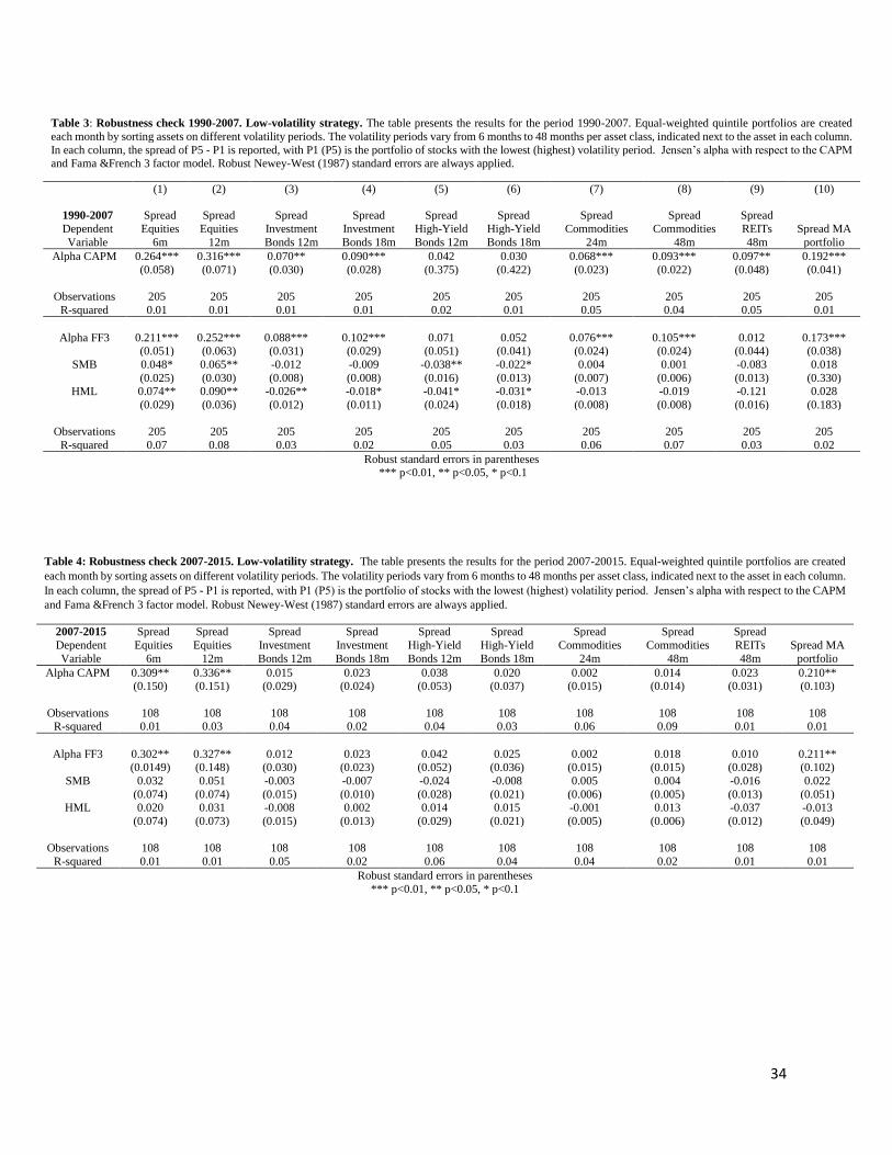
Section VI: Robustness checks

Low-volatility strategy

First, the robustness of the results low-volatility strategy are examined to other cross-sectional

factors. The regressions in this table are based on quintiles sorted on the same return volatility

periods as described in the above mentioned section ‘Results-Low volatility strategy’, however in

this case, time samples are taken into account. For all robustness checks the sample period is first

analyzed for 1990-2007 and then for 2007-2015. 2007 year indicates the year that the financial

crises has started, thus by splitting the time period in this way, the effect of financial crises on

factor investment strategies could be exploited. This robustness check is done for all individual

asset classes as well as for the multi-asest portfolio. When robsutness check for low-volatility

anomaly is tested, it can be concluded from tables 3 and 4 in the Appendix that high volatility

portfolios perform worse than low volatility portfolios. These results indicate that the low volatility

anomaly is robust for basing the return volatility on different time horizons. Furthermore, before

the financial crises in 2007, every individual asset class delivers higher alpha spread for both

CAPM and Fama and French 3 factor model in comparison to the after crises period 2007-2015.

Hence, the excess return that is generated by investing in this factor strategy decreases due to the

financial markets crash. The same observations can be drawn by look at table 11 that shows both

pre-crises Sharpe ratios and after crises Sharpe ratios. When the time horizon is split, higher Sharpe

26

ratios occure for pre-crises period. To conclude, persistent volatility effect is documented over

time.

Value

Contrary to the findings for low-volatility strategy, value strategy seems to actually perform

slightly better in the after-crises period of 2007-2015. Tables 6 and 7 report the alpha spreads per

individual assets and multi-asset portfolio, while table 12 presents the Sharpe ratios for both pre-

and after- crises period. As it can be interpreted from the tables, only the multi-asset portfolio seems

to generate slightly lower alpha spread in the post crises period and higher in the pre-crises period.

All individual assets have genereated higher alpha spread for the period 2007-2015. Consequently,

based on the findings above it can be established that value investing strategy works the best for

after crises period in comparison to low-volatility and momentum strategy.

Momentum

In order to check whether the results for the momentum anomaly hold and are robust, subsamples

are created for the same subperiods of 1990-2007 and 2008-2015 and examine whether each

quintile presents a consistent alpha throughout the two periods. Tables 9,10 and 13 deliver the

robustness check`s results for this market anomaly. All constants are significant for the subsample

1990-2007 that suggests mispricing of the investigated asset classes. However, after 2007, the

outburst of the recent financial crisis, only the high-yield bonds seem to have generated higher

alpha after the financial crises in comparison to the pre-crises period. On the contrary, commodities

seem to have fully crashed after the crises as the alpha spread becomes insignificant after the

financial collapse in 2007. All in all, the U.S. market shows that it could not recover from this

recession in terms of momentum yields.

Section VII: Concluding Remarks

The global financial crises provided unexpected breakthrough, namely that many of the different

asset classes have exposure to the same factors. Before the financial crises investors tended to

allocate to assets instead of to factors which have led investors to have a high exposure to

idiosyncratic risk, due to under diversification. Factor investing implementation was boosted due

to the relatively recent financial crisis and it will remain in the long-term as an investment strategy

27

since numerous empirical studies have proved that it can be taken advantage of. In this paper, the

strategies- low volatility, momentum, and value for the U.S. market were investigated. The aim of

this study was to investigate the impact of these market anomalies on a multi-asset portfolio and to

fill gaps in the financial literature. Some of the gaps in the existing arsenal of studies is that , studies

are mainly focusing on individual asset classes. Therefore, this paper analyzes the impact of factors

on a multi-asset portfolio. Furthermore, it investigates low-volatility effect on fixed-income market

and also analyzes the impact of value, momentum and low-volatility on REITs, which has never

been evaluated before. Additionaly, it examines the most recent time period starting from January

1990 till December 2015.

For low-volatility strategy it can be summarized that the multi-asset portfolio has the highest alpha

spread (0.387) and the highest Sharpe ratio (0.029) when in comparison to individual asset classes.

Equities sorted on 12 months and high- yield bonds sorted on 18 months volatility have the next

highest alpha spreads and Sharpe ratios. Investment bonds and commodities perform worse on this

investment strategy relative to the other assets by showing lower alpha spreads and Sharpe ratios.

In reference with the above paragraph, low-volatility strategy seems to work for the fixed-income

market as well. On the other hand, the low-volatility anomaly does not seem to work for REITs.

When analyzing value effect, it can be recapitulated that REITs have shown the highest alpha

spread (0.207) and the highest Sharpe ratio of 0.050. Second, high-yield bonds have produced the

next highest Sharpe ratio of 0.033, followed by the multi-asset portfolio`s one of 0.018. Third,

equities have Sharpe ratio of 0.013 followed by commodities. Last, investment grade bonds have

a negative Sharpe ratio and lowest alpha spread, hence value strategy is not applicable for this asset

class.

The results of momentum indicate that REITs have delivered the highest alpha spread (1.240) and

the highest Sharpe ratio of 0.280. Next, the multi-asset portfolio has generated the same Sharpe

ratio as equities (0.140), both sorted on 12 months cumulative returns. Following, investment

grade- and high-yield bonds have almost the same Sharpe ratios, with investment grade slightly

higher. In addition, investment grade bonds show higher alpha spread relative to high-yield bonds.

28

Last but not least, commodities sorted on 12 months CR and equities sorted on 6 months cumulative

returns deliver the lowest excess returns.

From the performed analysis, conclusions can be drawn as well for the individual asset classes.

Momentum in equities generates the highest Sharpe ratio, followed by low-volatility. For

investment grade bonds and high yield bonds, momentum generates highest Sharpe ratio, however

high yield bonds seems to have second best strategy value, while investment bonds`s second best

strategy would be low-volatility. For REIT, momentum seems to lead to the highest substantial

excess return, followed by value investment strategy. On the contrary, commodities seem to

generate highest excess return when low-volatility strategy is being applied. Last but not least, the

multi-asset portfolio has generated highest Sharpe ratio when momentum investing is used,

followed by low-volatility and value strategies.

Some limitations of this study should also be considered. First, transaction costs are not considered

in this report. Second, the conclusions are based on selected benchmark asset pricing models.

Further research could be conducted by utilizing other asset pricing models such as the Fama and

French (2015) 5 factor model. Third, the results obtained in this paper may not be valid for other

markets, because the features of each market vary. Fourth, this study was utilizing quintile

portfolios, hence another approach would be to rather use deciles, to stretch out the variation within

the data. Last, the research of this paper could be extended for other developed markets, as well as,

for developing markets.

These research findings will present a challenge to existing rational, behavioral and institutional

asset pricing theories that mainly focus on U.S. equities. This paper could be of interest to leading

asset management companies and investors who would like to maximize returns by better portfolio

diversification achieved by combining multi assets and taking advantage of exploiting market

anomalies as investment strategies.

29

Bibliography:

Ang, A., Hodrick, R. J., Xing, Y., and Zhang, X. (2006). The cross-section of volatility and

expected returns. The Journal of Finance, 61(1), 259-299.

Asness, C. S., Liew, J.M. and Stevens, R. (1997). Parallels between the crosssectional predictability

of stock and country returns. Journal of Portfolio Management 23, 79–87.

Asness, C. S., Moskowitz, Tobias J. and Pedersen, Lasse Heje. (2009). Value and Momentum

Everywhere. AFA 2010 Atlanta Meetings Paper.

Asness, C. S., Moskowitz, T. J., and Pedersen, L. H. (2013). Value and momentum everywhere.

Journal of Finance, 68(3), 929–985.

Baker, M., Bradley, B., and Wurgler, J. (2011). Benchmarks as limits to arbitrage: Understanding

the low-volatility anomaly. Financial Analysts Journal, 67(1), 40-54.

Baker, N. L., and Haugen, R. A. (2012). Low risk stocks outperform within all observable markets

of the world. Available at SSRN 2055431.

Bali, T. G., Cakici, N., and Whitelaw, R. F. (2011). Maxing out: Stocks as lotteries and the cross-

section of expected returns. Journal of Financial Economics, 99(2), 427-446.

Banz, R. W. (1981). The Relationship between Return and Market Value of Common Stocks.

Journal of Financial Economics, 9, 3-18.

Barberis, N., Shleifer, A., Vishny, R. (1998). A model of investor sentiment. Journal of financial

economics, 49(3), 307-343.

Barberis, N., Greenwood, R., Jin, L., and Shleifer, A. (2015). X-CAPM: An extrapolative capital

asset pricing model. Journal of Financial Economics, 115(1), 1-24.

Barberis, N., and Huang, M. (2008). Stocks as lotteries: The implications of probability weighting

for security prices. The American Economic Review, 98(5), 2066-2100.

Barroso, P, and P. Santa-Clara. (2013). Momentum has its moments. Working paper, available at

http://papers.ssrn.com/sol3/ papers.cfm?abstract_id=2041429.

Basu, S. (1977). Price-Earnings Ratios: A Test of the Efficient Market Hypothesis. The Journal of

Finance. Vol. 32, No. 3. 663—682.

Bender, J., et all. (2013). MSCI. Deploying Multi-Factor Index Allocations in Institutional

Portfolios

Berk and DeMarzo. (2014). Corporate finance (Global edition ed., Vol. Third edition). Essex:

Pearson.

Black, F. (1972). Capital Market Equilibrium with Restricted Borrowing. Journal of Business.

45(3), 444-54.

30

Black, F., Jensen, M., and Scholes, M. (1972). The Capital Asset Pricing Model: Some Empirical

Tests, Studies in the Theory of Capital Markets, Praeger, New York.

Blitz and Van Vliet. (2008). Global Tactical Cross-Asset Allocation: Applying Value and

Momentum across asset classes.

Blitz, D., and Van Vliet, P. (2007). The volatility effect: Lower risk without lower return. Journal

of Portfolio Management, 102-113.

Bollerslev, T., Engle, R. F., and Wooldridge, J. M. (1988). A capital asset pricing model with time-

varying covariances. The Journal of Political Economy, 116-131.

Chan, K., Chan, L., Jegadeesh, N., Lakonishok, J. (2006). Earnings Quality and Stock Returns.

The Journal of Business, 79(3), 1041-1082.

Cooper, M. J., R. C. Gutierrez, and A. Hameed. (2004). Market states and momentum, Journal of

Finance 59, 1345-1365. http://home.business.utah.edu/finmc/JOFI_12.pdf

Daniel and Moskowitz. (2014). Momentum Crashes. From:

http://papers.ssrn.com/sol3/papers.cfm?abstract_id=2632705

Daniel, K., and Titman, S. (1996). Evidence on the characteristics of cross sectional variation in

stock returns. http://www.nber.org/papers/w5604.pdf?new_window=1

Dasgupta, A., Prat, A., Verardo, M. (2011). Institutional trade persistence and long-term equity

returns. The Journal of Finance, 66(2):635-653.

De Bondt, W. F., and Thaler, R. H. (1994). Financial decision-making in markets and firms: A

behavioral perspective (No. w4777). National Bureau of Economic Research.

De Bondt, W., and Thaler, R. (1985). Does the stock market overreact? Journal of Finance 40, 793-

805. , 1987, Further evidence on investor overreaction and stock market seasonality, Journal of

Finance 42, 557-581.

De Long, J. B., Shleifer, A., Summers, L. H., and Waldmann, R. J. (1990). Positive feedback

investment strategies and destabilizing rational speculation. The Journal of Finance, 45(2), 379-

395.

Fama, E. F., and French, K. R. (1992). The cross-section of expected stock returns. The Journal of

Finance, 47(2), 427-465.

Fama, E. F., and French, K. R. (1993). Common risk factors in the returns on stocks and bonds.

Journal of Financial Economics, 33(1), 3-56.

Fama, E., and French, K. (1996). Multifactor explanations of asset pricing anomalies. Journal of

Finance, 51(1), 55-84.

Fama, E. F., and French, K. R. (2004). The capital asset pricing model: Theory and evidence. The

Journal of Economic Perspectives, 18 (3), 25-46.

31

Fama, E.F. French, K. R. (2015). A five-factor asset pricing model. Journal of Financial

Economics, 116 1-22.

Eraslan, V. (2013). Fama and French three-factor model: evidence from Istanbul stock exchange.

Business and Economics Research Journal, 4(2), 11.

Faff, R. (2004). A simple test of Fama and French model using daily data: Australian evidence.

Applied Financial Economics, 14(2), 83-92.

Falkenstein, E. G., (1994). Mutual funds, idiosyncratic variance, and asset returns. Dissertation,

Northwestern University.

Frazzini, A., and Pedersen, L. H. (2014). Betting against beta. Journal of Financial Economics, 111

(1), 1-25.

Gaunt, C. (2004). Size and book to market effects and the Fama French three factor asset pricing

model: Evidence from Australian Stock Market. Accounting and Finance, 44(1), 27-44.

Hong, H., Stein, J. (1999). A unified theory of underreaction, momentum trading, and overreaction

in asset markets. The Journal of Finance, 54(6):2143-2184, 1999.

Houweling, P. (2014). Factor Investing in the Corporate Bond Market.

Jagannathan, R., and Wang, Z. (1996). The conditional CAPM and the cross-section of expected

returns. The Journal of Finance, 51(1), 3-53.

Jegadeesh, N., Titman, S., (1993). Returns to buying winners and selling losers: Implications for

stock market efficiency. The Journal of Finance, 48(1):65-91, 1993.

Kahneman, D., and Tversky, A. (1979). Prospect theory: An analysis of decision under risk.

Econometrica: Journal of the econometric society, 263-291.

Kumar, A. (2009). Who gambles in the stock market? The Journal of Finance, 64(4), 1889-1933.

Lakonishok, J., Shleifer,A. and Vishny, R. (1994). “Contrarian Investment, Extrapolation, and

Risk.” Journal of Finance 49 (5): 1541-1578.

LaPorta, R., J. Lakonishok, A. Shleifer, and R. Vishny. (1997). Good news for value stocks: Further

evidence on market efficiency. Journal of Finance 52:859–74.

Larson, R. (2013). Hot Potato: Momentum as an Investment Strategy.

Lintner, J. (1965). The valuation of risk assets and the selection of risky investments in stock

portfolios and capital budgets. The review of economics and statistics, 13-37.

Lucas Jr, R. E. (1978). Asset prices in an exchange economy. Econometrica: Journal of the

Econometric Society, 1429-1445.

Markowitz, H.M. (1959). Portfolio selection: efficient diversification of investments. Wiley, New

York.

32

Merton, R. C. (1973). An intertemporal capital asset pricing model. Econometrica: Journal of the

Econometric Society, 867-887.

Piotroski, Joseph. (2000) Value investing: The use of historical financial statement information to

separate winners from losers, Journal of Accounting Research, 38, 1–41.

Rosenberg, B., K. Reid, and R. Lanstein. (1984). Persuasive evidence of market inefficiency,

Journal of Portfolio Management 11, 9-17.

Rouwenhorst, K. G. (1998). International momentum strategies. The Journal of Finance,53(1),

267-284.

Sharpe, W. F. (1964). Capital asset prices: A theory of market equilibrium under conditions of risk.

The Journal of Finance, 19(3), 425-442.

Shleifer, A. (2000). Inefficient markets: An introduction to behavioral finance. OUP Oxford.

Stivers, C., Sun, L. (2010). Cross-sectional return dispersion and time variation in value and

momentum premiums.

Treynor, J., L. (1962). Toward a Theory of Market Value of Risky Assets. Unpublished manuscript.

A final version was published in 1999, in Asset Pricing and Portfolio Performance: Models,

Strategy and Performance Metrics. Robert A. Korajczyk: Risk Books, pp. 15–22.

Vayanos and Woolley. (2013). An Institutional Theory of Momentum and Reversal. From:

https://academic.oup.com/rfs/article/26/5/1087/1593779/An-Institutional-Theory-ofMomentum-

and-Reversal

33

Appendix

Table 1: The table depicts summary statistics, including mean, standard deviation (sd), minimum value

(min) and maximum (max) value for selected variables. The period covers 1990-2015.

(1) (2) (3) (4) (5)

Variables N mean sd min max

Time 2,120,237 557.314 115.872 366 798

Excess Return Equities 935,896 0.275 601.448 -577,650 49,100

SMB 1,765,320 0.133 3.274 -17.170 22.080

HML 1,765,320 0.207 3.009 -11.250 12.910

Risk-free Rate 1,765,320 0.584 4.334 -17.230 11.350

ID 2,120,237 3,057.424 1,614.951 1 5,669

Date 2,120,237 16,184.510 2,772.857 10,958 20,454

Year 2,120,237 2,003.855 7.589 1990 2016

Month 2,120,237 6.485 3.459 1 12

Yield Investment Bonds 2,120,237 0.001 0.016 -0.070 0.056

Price Investment Bonds 2,120,237 103.665 5.501 83.718 115.14

Price High Yield Bonds 2,120,237 92.026 13.769 0 106.768

Yield High Yield Bonds 2,091,892 0.001 0.028 -0.169 0.132

Commodities Price 2,120,237 103.665 5.501 83.718 115.140

REITs Return 2,120,237 0.927 5.441 -29.852 33.721

Commodities Return 2,120,237 0.018 1.592 -7.000 5.569

Commodities Excess Return 1,765,320 -0.218 1.573 -7.150 5.569

REITs Excess Return 1,765,320 0.743 5.099 -29.932 33.711

Table 2: Low-volatility strategy. Equal-weighted quintile portfolios are created each month by sorting assets on different volatility periods. The volatility periods vary

from 6 months to 48 months per asset class, indicated next to the asset name in each column. In each column, the spread of P5 - P1 is reported, with P1 (P5) is the portfolio

of stocks with the lowest (highest) volatility period. Jensen’s alpha with respect to the CAPM and Fama &French 3 factor model. Robust Newey-West (1987) standard

errors are always applied. The sample period is January 1990 to December 2015.

(1) (2) (3) (4) (5) (6) (7) (8) (9) (10)

Dependent

Variable

Spread Equities

6m

Spread Equities

12m

Spread Investment

Bonds 12m

Spread Investment

Bonds 18m

Spread High-Yield

Bonds 12m

Spread High-Yield

Bonds 18m

Spread Commodities

24m

Spread Commodities

48m

Spread REITs

48m

Spread MA

portfolio

Alpha CAPM 0.278*** 0.323*** 0.052** 0.067*** 0.042 0.027 0.043 0.065*** -0.055 0.365*** (0.065) (0.069) (0.023) (0.020) (0.035) (0.027) (0.017) (0.015) (0.033) (0.046)

Observations 313 313 313 313 313 313 313 313 313 313 R-squared 0.01 0.01 0.02 0.01 0.01 0.01 0.04 0.05 0.01 0.01

Alpha FF3 0.267*** 0.309*** 0.057* 0.070* 0.051 0.267*** 0.043*** 0.066*** -0.031 0.387*** (0.065) (0.070) (0.023) (0.021) (0.036) (0.065) (0.016) (0.016) (0.030) (0.084)

SMB 0.035 0.049 -0.009 -0.007 -0.032 0.034 0.007 0.005 -0.062 -0.050

(0.026) (0.029) (0.007) (0.006) (0.013) (0.026) (0.005) (0.005) (0.010) (0.036) HML 0.037 0.041 -0.019** -0.010 -0.026 0.037 -0.002 -0.003 -0.079 -0.077

(0.032) (0.036) (0.009) (0.008) (0.017) (0.032) (0.006) (0.005) (0.011) (0.034)

Observations 313 313 313 313 313 313 313 313 313 313

R-squared 0.02 0.02 0.02 0.01 0.04 0.02 0.04 0.05 0.01 0.07

Robust standard errors in parentheses

*** p<0.01, ** p<0.05, * p<0.1

34

Table 4: Robustness check 2007-2015. Low-volatility strategy. The table presents the results for the period 2007-20015. Equal-weighted quintile portfolios are created

each month by sorting assets on different volatility periods. The volatility periods vary from 6 months to 48 months per asset class, indicated next to the asset in each column.

In each column, the spread of P5 - P1 is reported, with P1 (P5) is the portfolio of stocks with the lowest (highest) volatility period. Jensen’s alpha with respect to the CAPM

and Fama &French 3 factor model. Robust Newey-West (1987) standard errors are always applied.

2007-2015

Dependent

Variable

Spread

Equities

6m

Spread

Equities

12m

Spread

Investment

Bonds 12m

Spread

Investment

Bonds 18m

Spread

High-Yield

Bonds 12m

Spread

High-Yield

Bonds 18m

Spread

Commodities

24m

Spread

Commodities

48m

Spread

REITs

48m

Spread MA

portfolio

Alpha CAPM 0.309** 0.336** 0.015 0.023 0.038 0.020 0.002 0.014 0.023 0.210** (0.150) (0.151) (0.029) (0.024) (0.053) (0.037) (0.015) (0.014) (0.031) (0.103)

Observations 108 108 108 108 108 108 108 108 108 108 R-squared 0.01 0.03 0.04 0.02 0.04 0.03 0.06 0.09 0.01 0.01

Alpha FF3 0.302** 0.327** 0.012 0.023 0.042 0.025 0.002 0.018 0.010 0.211** (0.0149) (0.148) (0.030) (0.023) (0.052) (0.036) (0.015) (0.015) (0.028) (0.102)

SMB 0.032 0.051 -0.003 -0.007 -0.024 -0.008 0.005 0.004 -0.016 0.022

(0.074) (0.074) (0.015) (0.010) (0.028) (0.021) (0.006) (0.005) (0.013) (0.051) HML 0.020 0.031 -0.008 0.002 0.014 0.015 -0.001 0.013 -0.037 -0.013

(0.074) (0.073) (0.015) (0.013) (0.029) (0.021) (0.005) (0.006) (0.012) (0.049)

Observations 108 108 108 108 108 108 108 108 108 108

R-squared 0.01 0.01 0.05 0.02 0.06 0.04 0.04 0.02 0.01 0.01

Robust standard errors in parentheses

*** p<0.01, ** p<0.05, * p<0.1

Table 3: Robustness check 1990-2007. Low-volatility strategy. The table presents the results for the period 1990-2007. Equal-weighted quintile portfolios are created

each month by sorting assets on different volatility periods. The volatility periods vary from 6 months to 48 months per asset class, indicated next to the asset in each column.

In each column, the spread of P5 - P1 is reported, with P1 (P5) is the portfolio of stocks with the lowest (highest) volatility period. Jensen’s alpha with respect to the CAPM and Fama &French 3 factor model. Robust Newey-West (1987) standard errors are always applied.

(1) (2) (3) (4) (5) (6) (7) (8) (9) (10)

1990-2007

Dependent

Variable

Spread

Equities

6m

Spread

Equities

12m

Spread

Investment

Bonds 12m

Spread

Investment

Bonds 18m

Spread

High-Yield

Bonds 12m

Spread

High-Yield

Bonds 18m

Spread

Commodities

24m

Spread

Commodities

48m

Spread

REITs

48m

Spread MA

portfolio

Alpha CAPM 0.264*** 0.316*** 0.070** 0.090*** 0.042 0.030 0.068*** 0.093*** 0.097** 0.192***

(0.058) (0.071) (0.030) (0.028) (0.375) (0.422) (0.023) (0.022) (0.048) (0.041)

Observations 205 205 205 205 205 205 205 205 205 205

R-squared 0.01 0.01 0.01 0.01 0.02 0.01 0.05 0.04 0.05 0.01

Alpha FF3 0.211*** 0.252*** 0.088*** 0.102*** 0.071 0.052 0.076*** 0.105*** 0.012 0.173*** (0.051) (0.063) (0.031) (0.029) (0.051) (0.041) (0.024) (0.024) (0.044) (0.038)

SMB 0.048* 0.065** -0.012 -0.009 -0.038** -0.022* 0.004 0.001 -0.083 0.018

(0.025) (0.030) (0.008) (0.008) (0.016) (0.013) (0.007) (0.006) (0.013) (0.330) HML 0.074** 0.090** -0.026** -0.018* -0.041* -0.031* -0.013 -0.019 -0.121 0.028

(0.029) (0.036) (0.012) (0.011) (0.024) (0.018) (0.008) (0.008) (0.016) (0.183)

Observations 205 205 205 205 205 205 205 205 205 205

R-squared 0.07 0.08 0.03 0.02 0.05 0.03 0.06 0.07 0.03 0.02

Robust standard errors in parentheses *** p<0.01, ** p<0.05, * p<0.1

35

Table 6: Robustness check 1990-2007. Value strategy. The table presents the results for the sample of 1990-2007. Equal-weighted quintile portfolios are created each month by sorting assets on their value. Value for equities is calculated by taking the book-to-market ratio, while for all other assets a

standardized approach is applied. In each column, the spread of P5 - P1 is reported, with P1 (P5) is the portfolio of stocks with the lowest (highest)

value. Jensen’s alpha with respect to the CAPM and Fama &French 3 factor model. Robust Newey-West (1987) standard errors are always applied.

1990-2007 Dependent

Variable

(1) (2) (3) (4) (5) (6)

Spread

Equities Spread Investment

Bonds Spread High-Yield

Bonds Spread

Commodities Spread REITs

Spread MA

portfolio

Alpha CAPM 0.065** 0.065** 0.125** 0.076** 0.167** 0.188***

(0.032) (0.029) (0.053) (0.032) (0.076) (0.032)

Observations 205 205 205 205 205 205

R-squared 0.01 0.03 0.01 0.01 0.03 0.01

Alpha FF3 0.062** 0.075** 0.112* 0.085* 0.166** 0.192***

(0.031) (0.031) (0.058) (0.031) (0.077) (0.034) SMB 0.006 -0.023 0.004 -0.003 -0.017 -0.002

(0.011) (0.009) (0.017) (0.014) (0.018) (0.008)

HML -0.005 -0.130 0.020 0.014 -0.001 -0.005

(0.012) (0.011) (0.017) (0.016) (0.031) (0.011)

Observations 205 205 205 205 205 205 R-squared 0.01 0.06 0.01 0.01 0.02 0.01

Robust standard errors in parentheses

*** p<0.01, ** p<0.05, * p<0.1

Table 5: Value strategy. Equal-weighted quintile portfolios are created each month by sorting assets on their value. Value for equities is calculated

by taking the book-to-market ratio, while for all other assets a standardized approach is applied. In each column, the spread of P5 - P1 is reported, with P1 (P5) is the portfolio of stocks with the lowest (highest) value. Jensen’s alpha with respect to the CAPM and Fama &French 3 factor model. Robust Newey-West (1987) standard errors are always applied. The sample period is January 1990 to December 2015.

Dependent Variable

(1) (2) (3) (4) (5) (6)

Spread

Equities Spread Investment

Bonds Spread High-Yield

Bonds Spread

Commodities Spread REITs

Spread MA

portfolio

Alpha CAPM 0.117** 0.314 0.165*** 0.049 0.207** 0.187***

(0.028) (0.016) (0.049) (0.031) (0.064) (0.062)

Observations 313 313 313 313 313 247

R-squared 0.01 0.01 0.01 0.02 0.01 0.01

Alpha FF3 0.119*** 0.007 0.164** 0.048 0.207** 0.189***

(0.028) (0.019) (0.051) (0.033) (0.066) (0.020)

SMB -0.013 0.006 -0.002 0.003 0.013 -0.003 (0.010) (0.005) (0.015) (0.012) (0.019) (0.006)

HML -0.006 0.004 -0.004** -0.001 -0.001 -0.004

(0.010) (0.005) (0.013) (0.014) (0.026) (0.006)

Observations 313 313 313 313 313 247

R-squared 0.01 0.01 0.01 0.02 0.02 0.01

Robust standard errors in parentheses

*** p<0.01, ** p<0.05, * p<0.1

36

Table 8: Momentum strategy. Equal-weighted quintile portfolios are created each month by sorting assets on their cumulative returns

(either on 6 months cumulative return or on 12 months. Next to the asset name in each column, the cumulative returns period is specified. In

each column, the spread of P5 - P1 is reported, with P1 (P5) is the portfolio of stocks with the lowest (highest) cumulative returns. Jensen’s

alpha with respect to the CAPM and Fama &French 3 factor model. Robust Newey-West (1987) standard errors are always applied. The sample period is January 1990 to December 2015.

(1) (2) (3) (4) (5) (6) (7) (8)

Dependent Variable

Spread

Equities 6m

Spread

Equities 12m

Spread

Investment Bonds 12m

Spread

High-Yield Bonds 12m

Spread

Commodities 12m

Spread

REITs 12m

Spread MA portfolio 6m

Spread MA

portfolio 12m

Alpha CAPM 0.023 1.030*** 0.539** 0.470*** 0.027 1.230*** 0.067 0.918**

(0.367) (0.326) (0.114) (0.135) (0.019) (0.024) (0.247) (0.307)

Observations 307 307 313 313 313 313 313 296

R-squared 0.01 0.02 0.01 0.01 0.01 0.01 0.01 0.01

Alpha FF3 0.039 1.120*** 0.545*** 0.465*** 0.026 1.240*** 0.097 1.000***

(0.364) (0.315) (0.117) (0.139) (0.019) (0.024) (0.250) (0.296) SMB -0.107 -0.053 0.048 -0.024 -0.007 -0.011 -0.060 -0.038

(0.164) (0.140) (0.045) (0.044) (0.008) (0.008) (0.099) (0.133)

HML -0.185 -0.255 -0.029 0.010 0.002 -0.004 -0.100 -0.236

(0.201) (0.165) (0.049) (0.058) (0.007) (0.008) (0.126) (0.160)

Observations 307 307 313 313 313 313 313 296

R-squared 0.01 0.02 0.02 0.01 0.01 0.01 0.01 0.02

Robust standard errors in parentheses *** p<0.01, ** p<0.05, * p<0.1

Table 7: Robustness check 2007-2015. Value strategy. The table presents the results for the sample of 2007-2015. Equal-weighted quintile

portfolios are created each month by sorting assets on their value. Value for equities is calculated by taking the book-to-market ratio, while for all

other assets a standardized approach is applied. In each column, the spread of P5 - P1 is reported, with P1 (P5) is the portfolio of stocks with the lowest (highest) value. Jensen’s alpha with respect to the CAPM and Fama &French 3 factor model. Robust Newey-West (1987) standard errors are always applied.

2007-2015 Dependent Variable

(1) (2) (3) (4) (5) (6)

Spread

Equities Spread Investment

Bonds Spread High-Yield

Bonds Spread

Commodities Spread REITs

Spread MA

portfolio

Alpha CAPM 0.213*** 0.127** 0.235** 0.235** 0.289** 0.186***

(0.054) (0.056) (0.099) (0.123) (0.123) (0.037)

Observations 108 108 108 108 108 108

R-squared 0.01 0.02 0.02 0.01 0.01 0.01

Alpha FF3 0.210*** 0.130** 0.241** 0.001 0.281** 0.186***

(0.052) (0.058) (0.102) (0.067) (0.127) (0.037)

SMB 0.037 0.017 -0.009 0.016 0.002 -0.015 (0.023) (0.025) (0.053) (0.035) (0.049) (0.014)

HML 0.006 0.009 0.017 0.003 0.024 -0.001 (0.018) (0.026) (0.036) (0.024) (0.047) (0.016)

Observations 108 108 108 108 108 108 R-squared 0.02 0.02 0.02 0.05 0.01 0.02

Robust standard errors in parentheses

*** p<0.01, ** p<0.05, * p<0.1

37

Table 10: Robustness check 2007-2015. Momentum strategy. The table reports the results for the sample 2007-2015. Equal-weighted

quintile portfolios are created each month by sorting assets on their cumulative returns (either on 6 months cumulative return or on 12 months. Next to the asset name in each column, the cumulative returns period is specified. In each column, the spread of P5 - P1 is reported, with P1

(P5) is the portfolio of stocks with the lowest (highest) cumulative returns. Jensen’s alpha with respect to the CAPM and Fama &French 3 factor model. Robust Newey-West (1987) standard errors are always applied.

(1) (2) (3) (4) (5) (6) (7) (8)

2007-2015

Dependent

Variable

Spread Equities

6m

Spread Equities

12m

Spread Investment

Bonds 12m

Spread High-Yield

Bonds 12m

Spread Commodities

12m

Spread REITs

12m

Spread MA

portfolio 6m

Spread MA portfolio

12m

Alpha CAPM 0.109 0.823 0.527** 0.521*** 0.011 1.240*** 0.195 0.681**

(0.687) (0.535) (0.196) (0.252) (0.036) (0.041) (0.461) (0.506) Observations 109 109 109 109 109 109 109 109

R-squared 0.01 0.01 0.01 0.01 0.02 0.01 0.01 0.01

Alpha FF3 0.183 0.855 0.547*** 0.543** -0.007 1.230*** 0.252 0.719

(0.652) (0.535) (0.193) (0.247) (0.036) (0.042) (0.447) (0.501) SMB 0.085 0.086 0.012 -0.015 -0.003 0.032 0.024 0.127

(0.366) (0.305) (0.097) (0.134) (0.016) (0.022) (0.238) (0.299)

HML 0.210 0.087 0.062 0.067 0.011 0.010 0.165 0.100 (0.232) (0.254) (0.096) (0.105) (0.013) (0.015) (0.233) (0.236)

Observations 109 109 109 109 109 109 109 109 R-squared 0.01 0.01 0.02 0.01 0.02 0.03 0.01 0.02

Robust standard errors in parentheses

*** p<0.01, ** p<0.05, * p<0.1

Table 9: Robustness check 1990-2007. Momentum strategy. The table reports the results for the sample 1990-2007. Equal-weighted

quintile portfolios are created each month by sorting assets on their cumulative returns (either on 6 months cumulative return or on 12 months.

Next to the asset name in each column, the cumulative returns period is specified. In each column, the spread of P5 - P1 is reported, with P1

(P5) is the portfolio of stocks with the lowest (highest) cumulative returns. Jensen’s alpha with respect to the CAPM and Fama &French 3

factor model. Robust Newey-West (1987) standard errors are always applied.

(1) (2) (3) (4) (5) (6) (7) (8) 1990-2007

Dependent

Variable

Spread

Equities

6m

Spread

Equities

12m

Spread

Investment

Bonds 12m

Spread

High-Yield

Bonds 12m

Spread

Commodities

12m

Spread

REITs

12m

Spread MA

portfolio 6m

Spread MA

portfolio

12m

Alpha CAPM 0.104 1.130*** 0.536*** 0.434*** 0.046** 1.230*** 0.002 1.040***

(0.434) (0.422) (0.139) (0.158) (0.022) (0.029) (0.292) (0.393)

Observations 204 204 204 204 204 204 204 204

R-squared 0.01 0.01 0.02 0.01 0.01 0.01 0.01 0.01

Alpha FF3 0.226 1.560*** 0.546*** 0.423*** 0.045** 1.240*** 0.185 1.440***

(0.367) (0.352) (0.144) (0.161) (0.023) (0.031) (0.271) (0.321)

SMB -0.224 -0.169 0.061 -0.024 -0.008 0.007 -0.131 -0.154 (0.174) (0.153) (0.051) (0.050) (0.008) (0.009) (0.107) (0.144)

HML -0.431 -0.506 -0.021 0.018 0.002 -0.008 -0.271 -0.473

(0.219) (0.199) (0.057) (0.069) (0.007) (0.012) (0.135) (0.193)

Observations 204 204 204 204 204 204 204 204

R-squared 0.05 0.06 0.03 0.01 0.01 0.01 0.03 0.07

Robust standard errors in parentheses *** p<0.01, ** p<0.05, * p<0.1

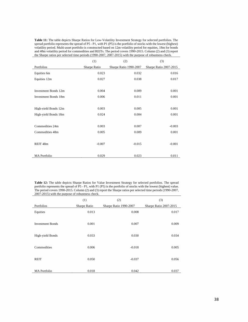
38

Table 12: The table depicts Sharpe Ratios for Value Investment Strategy for selected portfolios. The spread

portfolio represents the spread of P5 - P1, with P1 (P5) is the portfolio of stocks with the lowest (highest) value.

The period covers 1990-2015. Column (2) and (3) report the Sharpe ratios per selected time periods (1990-2007, 2007-2015) with the purpose of robustness check.

(1) (2) (3)

Portfolios Sharpe Ratio Sharpe Ratio 1990-2007 Sharpe Ratio 2007-2015

Equities 0.013 0.008 0.017

Investment Bonds 0.001 0.007 0.009

High-yield Bonds 0.033 0.030 0.034

Commodities 0.006 -0.018 0.005

REIT 0.050 -0.037 0.056

MA Portfolio 0.018 0.042 0.037

Table 11: The table depicts Sharpe Ratios for Low-Volatility Investment Strategy for selected portfolios. The

spread portfolio represents the spread of P5 - P1, with P1 (P5) is the portfolio of stocks with the lowest (highest)

volatility period. Multi-asset portfolio is constructed based on 12m volatility period for equities, 18m for bonds and 48m volatility period for commodities and REITs. The period covers 1990-2015. Column (2) and (3) report

the Sharpe ratios per selected time periods (1990-2007, 2007-2015) with the purpose of robustness check.

(1) (2) (3)

Portfolios Sharpe Ratio Sharpe Ratio 1990-2007 Sharpe Ratio 2007-2015

Equities 6m 0.023 0.032 0.016

Equities 12m 0.027 0.038 0.017

Investment Bonds 12m 0.004 0.009 0.001

Investment Bonds 18m 0.006 0.011 0.001

High-yield Bonds 12m 0.003 0.005 0.001

High-yield Bonds 18m 0.024 0.004 0.001

Commodities 24m 0.003 0.007 -0.003

Commodities 48m 0.005 0.009 0.001

REIT 48m -0.007 -0.015 -0.001

MA Portfolio 0.029 0.023 0.011

39

Table 13: The table depicts Sharpe Ratios for Momentum Investment Strategy for selected portfolios. The spread portfolio represents 'winners'-'losers' portfolios (P5-P1). 6m and 12m indicate the period on what period of cumulative

returns a particular asset is sorted The period covers 1990-2015. Column (2) and (3) report the Sharpe ratios per

selected time periods (1990-2007, 2007-2015) with the purpose of robustness check.

(1) (2) (3)

Portfolios Sharpe Ratio Sharpe Ratio 1990-2007 Sharpe Ratio 2007-2015

Equities 6m 0.002 -0.006 0.013

Equities 12m 0.140 0.176 0.103

Investment Bonds 12m 0.056 0.065 0.046

High-yield Bonds 12m 0.055 0.051 0.054

Commodities 12m 0.003 0.006 -0.001

REIT 12m 0.280 0.296 0.263

MA Portfolio 12m 0.140 0.175 0.086