Multi-Armed Bandits (MABs) - Purdue University Bandits (MABs) CS57300 - Data Mining Fall 2016 ......

Multi-Armed Bandits (MABs)

CS57300 - Data MiningFall 2016

Instructor: Bruno Ribeiro

} So far we have seen how to:◦ Test a hypothesis in batches (A/B testing)◦ Test multiple hypotheses (Paul the Octopus-style)◦ Stop a hypothesis test before experiment is over

2

Recap last two classes

© 2016 Bruno Ribeiro

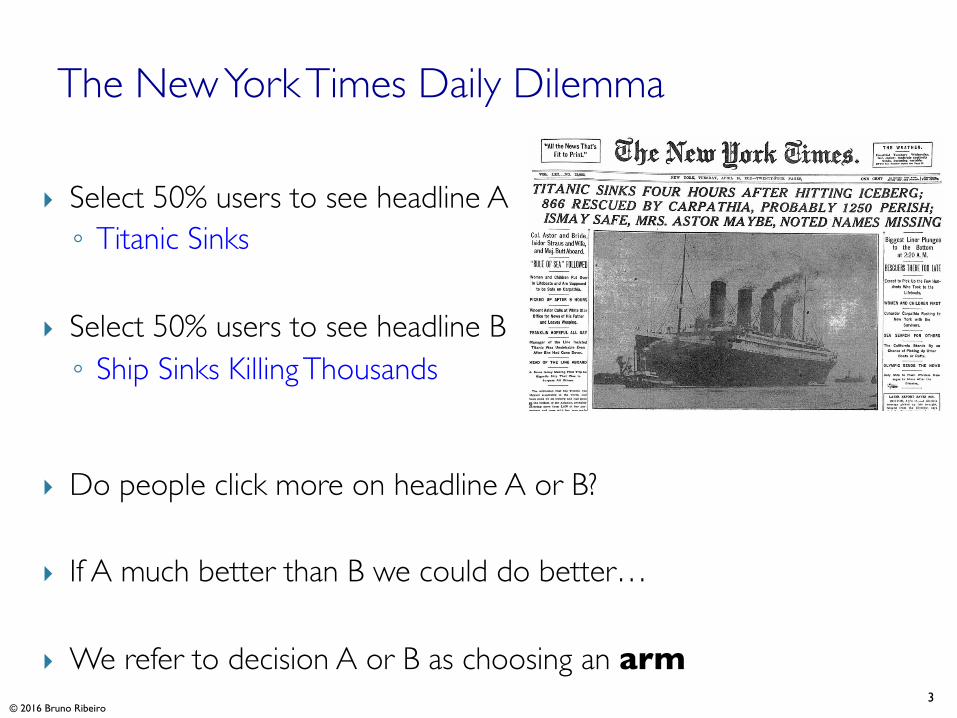
} Select 50% users to see headline A◦ Titanic Sinks

} Select 50% users to see headline B◦ Ship Sinks Killing Thousands

} Do people click more on headline A or B?

} If A much better than B we could do better…

} We refer to decision A or B as choosing an arm

The New York Times Daily Dilemma

3© 2016 Bruno Ribeiro

} Sometimes we don’t only want to quickly find whether hypothesis A is better than hypothesis B

} We really want to use the best-looking hypothesis at any point in time

} Deciding if H0 should be rejected is irrelevant

4

Truth is…


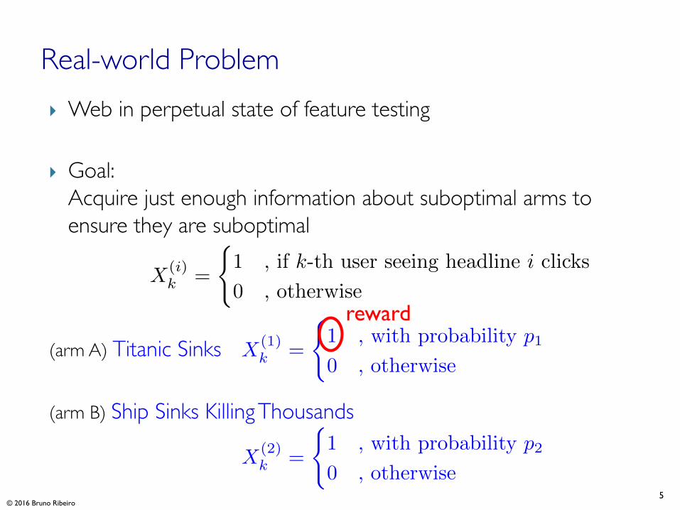
} Web in perpetual state of feature testing

} Goal: Acquire just enough information about suboptimal arms to ensure they are suboptimal

(arm A) Titanic Sinks

(arm B) Ship Sinks Killing Thousands

5

Real-world Problem

X(i)k =

(1 , if k-th user seeing headline i clicks

0 , otherwise

X(1)k =

(1 , with probability p10 , otherwise

X(2)k =


reward


6

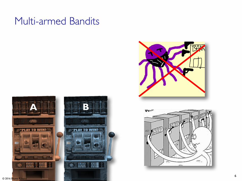
Multi-armed Bandits

A B


} Play t times

} Each time choose arm i∈{1,2}

} Goal: Maximize total expected reward

7

Multi-armed Bandit Dynamics

A

B

X(1)k =


X(2)k =


π is a vector of the arms we playπt is the t-th played arm


RT =TX

t=1

X(⇡t)n⇡t (t)

,

where ni(t) =tX

h=1

1{⇡h = i}

k-th time arm A is played

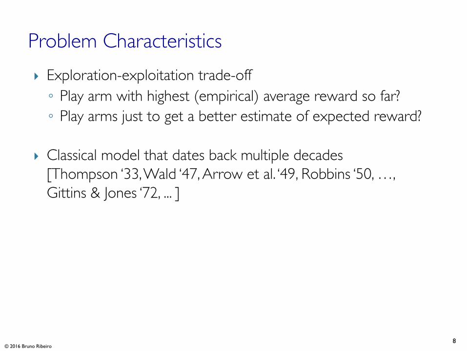
} Exploration-exploitation trade-off◦ Play arm with highest (empirical) average reward so far?◦ Play arms just to get a better estimate of expected reward?

} Classical model that dates back multiple decades [Thompson ‘33, Wald ‘47, Arrow et al. ‘49, Robbins ‘50, …, Gittins & Jones ‘72, ... ]

8

Problem Characteristics


9

Formal Bandit Definition

Markov chain: P [X(i)k |X(i)

k�1, X(i)k�2, . . .] = P [X(i)

k |X(i)k�1]

• K � 2 arms

• Pulling ni times arm i produces rewards X

(i)1 , . . . , X

(i)ni

with (unknown) joint distribution f(x1, . . . , xni |✓i), ✓i 2 ⇥

• At time t � ni(t) we know X

(i)1 , . . . , X

(i)ni(t)

,

where ni(t) is the number of pulls of arm i at time t.

• Many formulations assume X

(i)1 , . . . , X

(i)ni(t)

form a Markov chain


• Most applications assume i.i.d. draws P [X(i)k |X(i)

k�1, . . .] = P [X(i)k ]

(A1) only one arm is operated each time

(A2) rewards in arms not used remain froze

(A3) arms are independent

(A4) frozen arms contribute no reward

10

Assumptions (can be easily violated in practice)


11

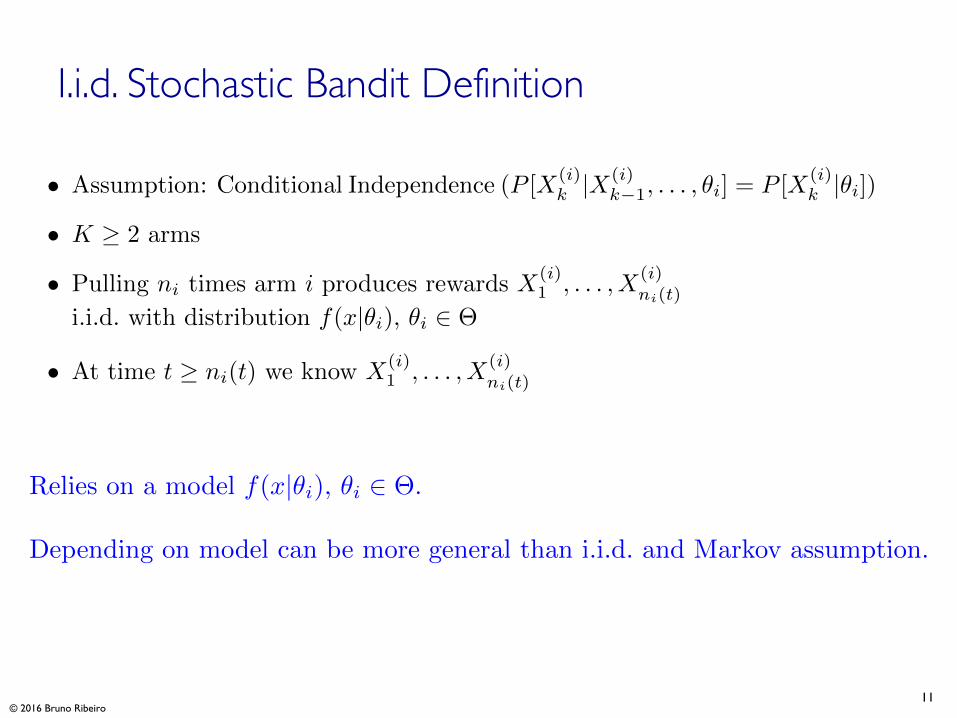
I.i.d. Stochastic Bandit Definition


• Assumption: Conditional Independence (P [X

(i)k |X(i)

k�1, . . . , ✓i] = P [X

(i)k |✓i])

• K � 2 arms

• Pulling ni times arm i produces rewards X

(i)1 , . . . , X

(i)ni(t)

i.i.d. with distribution f(x|✓i), ✓i 2 ⇥

• At time t � ni(t) we know X

(i)1 , . . . , X

(i)ni(t)

Relies on a model f(x|✓i), ✓i 2 ⇥.

Depending on model can be more general than i.i.d. and Markov assumption.

12

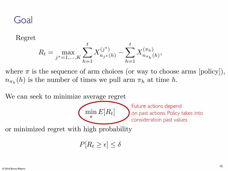
Goal


Future actions dependon past actions. Policy takes intoconsideration past values

Regret

Rt = max

j?=1,...,K

tX

h=1

X(j?)nj? (h)

�tX

h=1

X(⇡h)n⇡h

(h),

where ⇡ is the sequence of arm choices (or way to choose arms [policy]),

n⇡h(h) is the number of times we pull arm ⇡h at time h.

We can seek to minimize average regret

min

⇡E[Rt]

or minimized regret with high probability

P [Rt � ✏] �

13

Regret Growth with i.i.d. Rewards

Optimal policy Chosen policy

• Standard deviation of empirical

Pni

k=1 X(i)k grows like

pt

• Thus, at best E[Rt] /pt

• Rather, we minimize over ⇡ w.r.t. best policy (Pseudo-regret)

¯Rt = max

i?=1,...,KE

"nX

h=1

X(i?)ni? (h)

�nX

h=1

X(⇡h)n⇡h

(h)

#


14

Reward Definitions


15

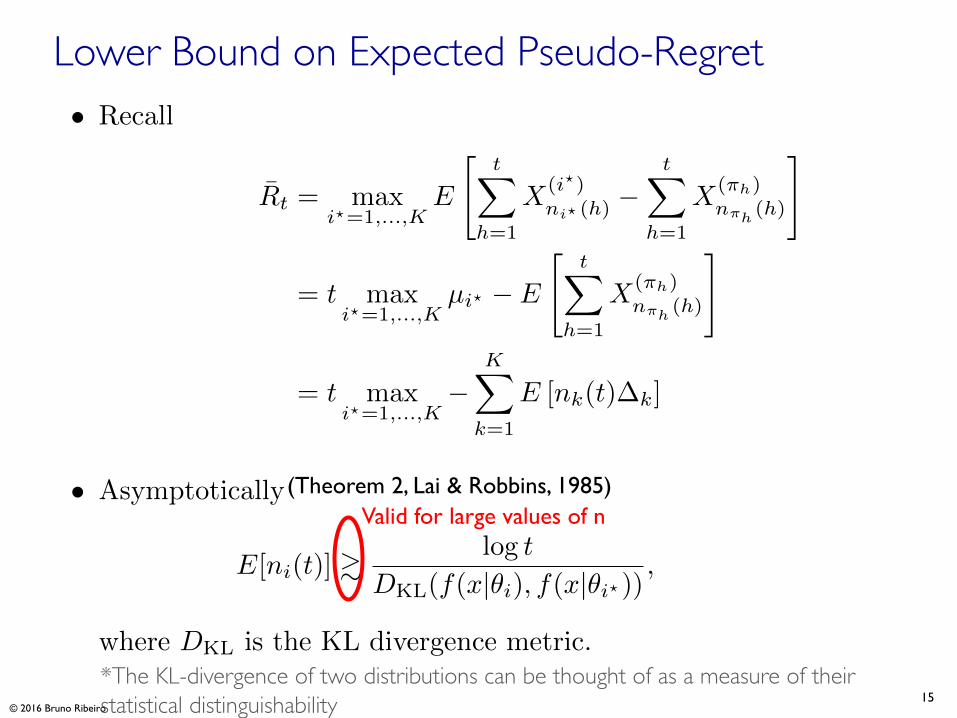
Lower Bound on Expected Pseudo-Regret

*The KL-divergence of two distributions can be thought of as a measure of their statistical distinguishability

(Theorem 2, Lai & Robbins, 1985)Valid for large values of n


• Recall

¯

Rt = max

i?=1,...,KE

"tX

h=1

X

(i?)ni? (h)

�tX

h=1

X

(⇡h)n⇡h

(h)

#

= t max

i?=1,...,Kµi? � E

"tX

h=1

X

(⇡h)n⇡h

(h)

#

= t max

i?=1,...,K�

KX

k=1

E [nk(t)�k]

• Asymptotically

E[ni(t)] &log t

DKL(f(x|✓i), f(x|✓i?)),

where DKL is the KL divergence metric.

16

Playing Strategies


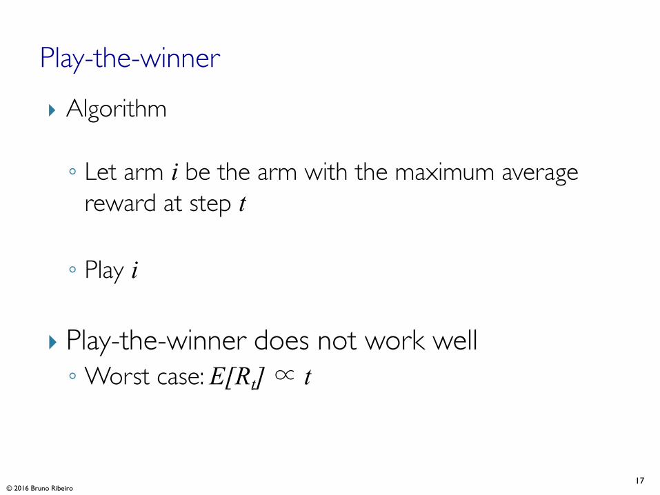
} Algorithm

◦ Let arm i be the arm with the maximum average reward at step t

◦ Play i

} Play-the-winner does not work well◦Worst case: E[Rt]∝ t

17

Play-the-winner


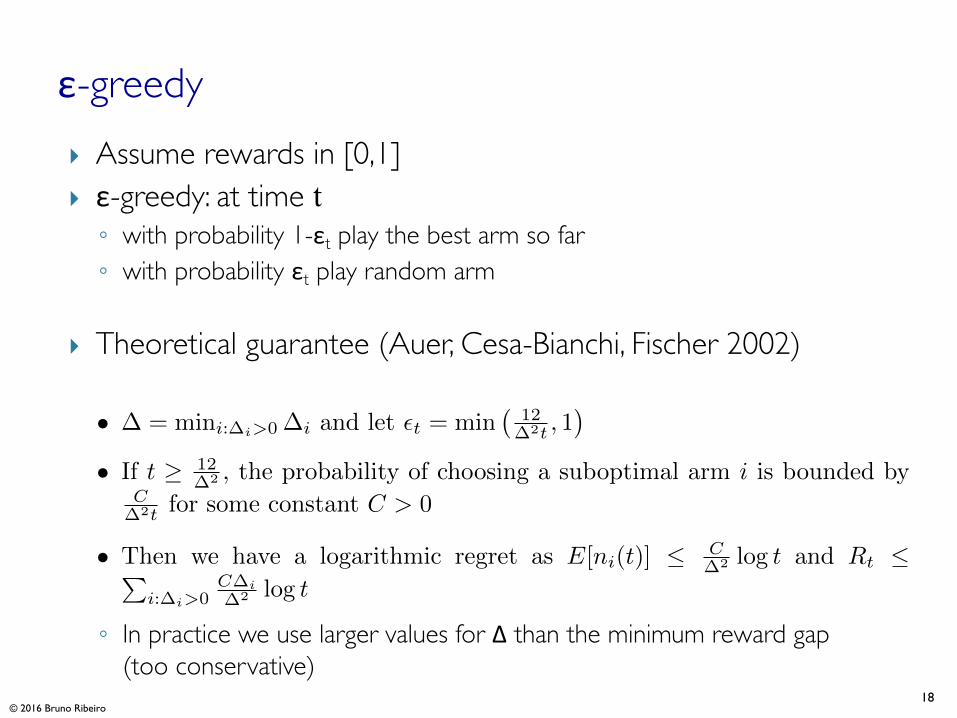
} Assume rewards in [0,1]} ε-greedy: at time t◦ with probability 1-εt play the best arm so far◦ with probability εt play random arm

} Theoretical guarantee (Auer, Cesa-Bianchi, Fischer 2002)

◦ In practice we use larger values for Δ than the minimum reward gap (too conservative)

18

ε-greedy

• � = mini:�i>0 �i and let ✏t = min

�12�2t , 1

�

• If t � 12�2 , the probability of choosing a suboptimal arm i is bounded by

C�2t for some constant C > 0

• Then we have a logarithmic regret as E[ni(t)] C�2 log t and Rt P

i:�i>0C�i�2 log t


} For K > 2 arms we play suboptimal arms with same probability

} Very sensitive to high variance rewards

} Real-world performance worst than next algorithm (UCB1)

19

Problems of ε-greedy


} Using a probabilistic argument we can provide an upper bound of the expected reward for arm i=1,…,K with a given level of confidence

} Strategy: play arm with largest upper bound

} Algorithm known as Upper Confidence Bound 1 (UCB1)

20

Optimism in Face of Uncertainty (UCB)


} UCB1 algorithm

◦ t total arm plays◦ Let◦ Gives algorithm:� Play arm i with largest

21

Using the Chernoff-HoeffdingTheorem

1-1/t

1

ni(t)

ni(t)X

k=1

Xk +

s2 log t

ni(t)

Let X1, . . . , Xni be i.i.d. rewards from arm i with distribution

bounded in [0, 1], then for any ✏ 2 (0, 1)

P

"niX

k=1

Xk niE[X1]� ✏

# exp

✓�2✏2

ni

◆

✏ =p2ni(t) log t

Why: P2

4 1

ni(t)

ni(t)X

k=1

Xk +

s2 log t

ni(t) E[X1]

3

5 t�4


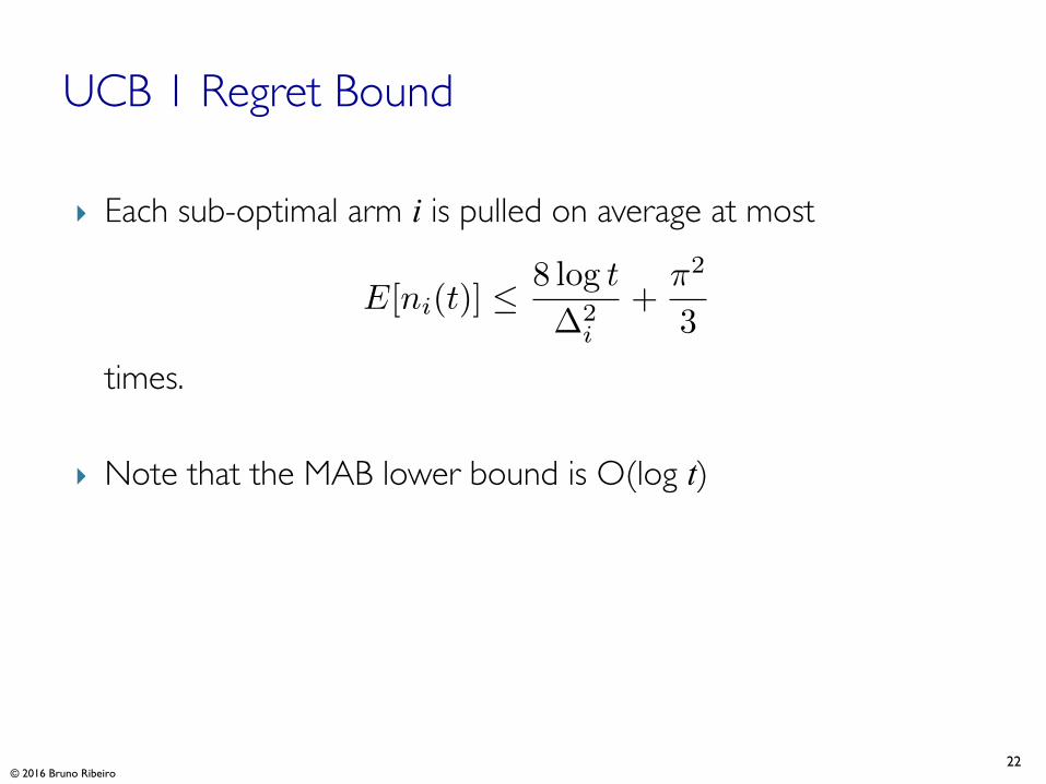
} Each sub-optimal arm i is pulled on average at most

times.

} Note that the MAB lower bound is O(log t)

22

UCB 1 Regret Bound

E[ni(t)] 8 log t

�

2i

+

⇡2

3


} Use Empirical Bernstein’s inequality

} Play arm i at time t if i has the maximim

23

Improving Bound ➡ Smaller Regret


} Optimal solutions via stochastic dynamic programming ◦ Gittins index

} Suffer from Incomplete Learning (Brezzi and Lai 2000, Kumar and Varaiya 1986)

◦ Playing the wrong arm foreverwith non-zero probability◦ One more reason to be warry of average rewards

} Only applicable to infinite horizon & complex to compute

} Poor performance on real-world problems

Forever Wrong

24

Optimal Solution?


} Thompson sampling◦ Strategy: select arm i according to posterior probability

◦ Can be used in complex problems (dependent priors, complex actions, dependent rewards)

◦ Great real-world performance

◦ Great regret bounds

25

Bayesian Bandits (continuing from last class)


26

Bernoulli Bandits


• Let µi 2 (0, 1)

• Reward of arm i = 1, . . . ,K at step k is X(i)k ⇠ Bernoulli(µi)

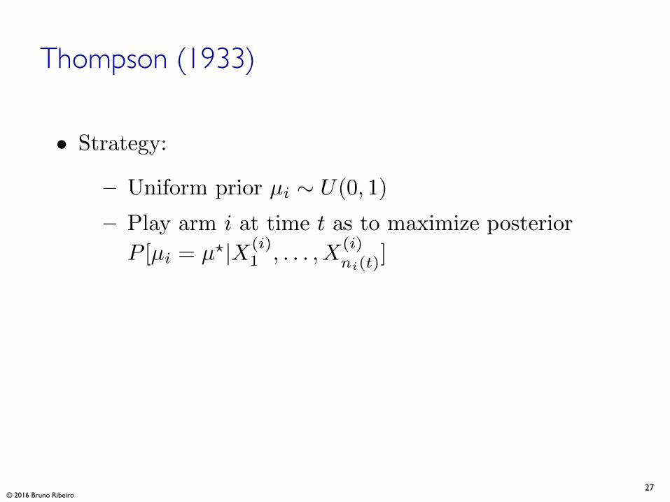
• Strategy:

– Uniform prior µi ⇠ U(0, 1)

– Play arm i at time t as to maximize posterior

P [µi = µ?|X(i)1 , . . . , X(i)

ni(t)]

– Typically simpler randomized strategy:

play i with probability P [µi = µ?|X(i)1 , . . . , X(i)

ni(t)]

27

Thompson (1933)


28

Bernoulli rewards + Beta priors

Beta distribution PDF

wikipedia


Yt|It ⇠ Bernoulli(µIt)

Prior: Beta distribution

P [µi|↵,�] =µ↵�1i (1� µi)

��1

R 10 p↵�1

(1� p)��1dp

Posterior µi ⇠ Beta(↵+

Ptk=1 Yk1{Ik = i},� +

Ptk=1(1� Yk)1{Ik = i})

29

Thompson Algorithm (for Bernoulli rewards)

Binomial Distribution

Number of Correct Predictions

Dens

ity

0 2 4 6 8 10 12

0.00

0.05

0.10

0.15

0.20

Yt© 2016 Bruno Ribeiro

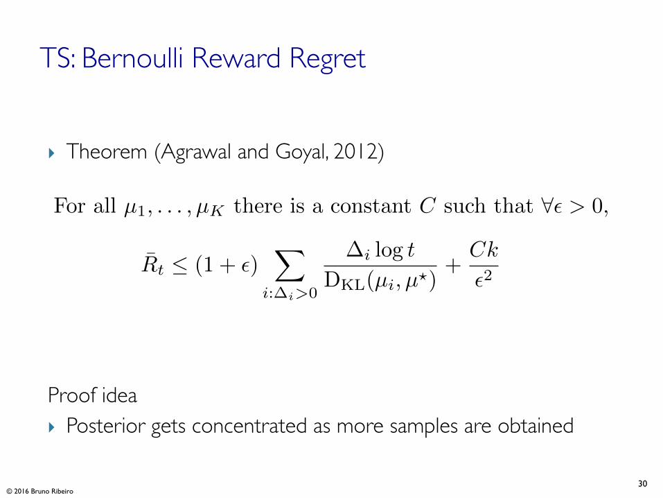
} Theorem (Agrawal and Goyal, 2012)

30

TS: Bernoulli Reward Regret

Proof idea} Posterior gets concentrated as more samples are obtained


For all µ1, . . . , µK there is a constant C such that 8✏ > 0,

¯Rt (1 + ✏)X

i:�i>0

�i log t

DKL(µi, µ?)

+

Ck

✏2

} Facebook & Linkedin use two-sample hypothesis tests instead of MAB. Why?

} More generally, which MAB assumptions often does not hold in real-life applications?

31

Some Shortcomings of MAB


(A2) rewards in arms not used remain froze Recommendation influence users

(A3) arms are independentUsers are influenced by what they see and by each other

32

Assumptions most violated in practice


33

Advanced Topic

(Contextual Bandits)

} Bandits with side information

} We know reader subscribes to magazine

} Headline A may be more successful in this subpopulation◦ Titanic Sinks

} Headline B better for general population◦ Ship Sinks Killing Thousands

34

Contextual Bandits


} Consider a hash (random function) with deterministic projection h:{0,1}n → ℝm

} At each play:

some useful assumptions about f

35

Contextual Bandits: Problem Formulation

User features Headline features (context)

Learned from observations(e.g. recursive least squares)


1. Observe features Xt 2 X

2. Choose arm it 2 {1, . . . ,K}

3. In theory we will get reward Yt = f(h(xt, zit)|✓) + ✏t

} First we build model

36

Contextual Bandits (linear model)


37

Thompson Sampling for Linear Contextual Bandits 1/2


Assume noise is Gaussian

✏t ⇠ N(0,�2)

and that ✓ has prior

✓ ⇠ N(0,2I)

The posterior distribution of ✓ is given by

p(✓|Xt, ~Yt) = N(

ˆ✓t,⌃t)

where

⌃t = �I +XTtXt,

where � =

�2

2 .

38

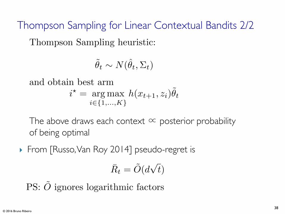
Thompson Sampling for Linear Contextual Bandits 2/2

} From [Russo, Van Roy 2014] pseudo-regret is

The above draws each context ∝ posterior probability of being optimal

Rt = O(dpt)


Thompson Sampling heuristic:

˜

✓t ⇠ N(

ˆ

✓t,⌃t)

and obtain best arm

i

?= argmax

i2{1,...,K}h(xt+1, zi)

˜

✓t

39

Example

Effectiveness of ad may depend on consumer

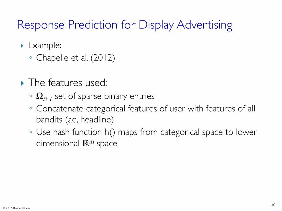
} Example:◦ Chapelle et al. (2012)

} The features used: ◦ Ωt+1 set of sparse binary entries◦ Concatenate categorical features of user with features of all

bandits (ad, headline) ◦ Use hash function h() maps from categorical space to lower

dimensional ℝm space

40

Response Prediction for Display Advertising


41

Algorithm for Display Advertising


Goal: maximize the number of clicks or conversions

Model: Logistic regression

P [Yt = 1|xt, zIt , ✓] =1

1 + exp(�✓

Th(xt, zIt))

Response prediction based on training

set ⌦

0t = {(xk, zIk , yk)}k=1,...,t

ˆ

✓ = argmin

↵2Rm

�

2

k↵k2 +tX

k=1

log(1 + exp(�yk↵Th(xk, zIk))

42

Display Ads (cont)


If prior ✓ ⇠ N(0,

1� I), the posterior P [✓|D]

has no closed form expression but we can use the

Laplace approximation of the integral

P [✓|D] = N(

ˆ

✓, diag(qi)�1

)

where

qi =

tX

j=1

w

2j,ipj(1� pj) with pj = (1 + exp(�ˆ

✓

Th(xj , zIj )))

�1

and wj = h(xj , zIj )

43

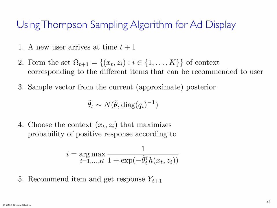
Using Thompson Sampling Algorithm for Ad Display


1. A new user arrives at time t+ 1

2. Form the set ⌦t+1 = {(xt, zi) : i 2 {1, . . . ,K}} of context

corresponding to the di↵erent items that can be recommended to user

3. Sample vector from the current (approximate) posterior

˜

✓t ⇠ N(

ˆ

✓, diag(qi)�1

)

4. Choose the context (xt, zi) that maximizes

probability of positive response according to

i = argmax

i=1,...,K

1

1 + exp(�˜

✓

Tth(xt, zi))

5. Recommend item and get response Yt+1

Multi-Armed Bandits (MABs) - Purdue University Bandits (MABs) CS57300 - Data Mining Fall 2016 ......

Documents

Transcript of Multi-Armed Bandits (MABs) - Purdue University Bandits (MABs) CS57300 - Data Mining Fall 2016 ......