http://www.diva-portal.org

Postprint

This is the accepted version of a paper published in Journal of Biophotonics. This paper has been peer-reviewed but does not include the final publisher proof-corrections or journal pagination.

Citation for the original published paper (version of record):

Mücksch, J., Spielmann, T., Sisamakis, E., Widengren, J. (2015)

Transient state imaging of live cells using single plane illumination and arbitrary duty cycle

excitation pulse trains.

Journal of Biophotonics, 8(5): 392-400

http://dx.doi.org/10.1002/jbio.201400015

Access to the published version may require subscription.

N.B. When citing this work, cite the original published paper.

Permanent link to this version:http://urn.kb.se/resolve?urn=urn:nbn:se:kth:diva-170699

1

Transient State Imaging of live cells by Single Plane

Illumination Microscopy.

Jonas Mücksch†, Thiemo Spielmann

†, Evangelos Sisamakis and Jerker Widengren

‡

Experimental Biomolecular Physics, Department of Applied Physics,

Royal Institute of Technology, Stockholm, Sweden

† The authors contributed equally,

‡ Corresponding author:

Jerker Widengren

Experimental Biomolecular Physics

Department of Applied Physics

Royal Institute of Technology,

Albanova University Center,

106 91 Stockholm, Sweden

Phone: +46855378030

Email: jerker@biomolphysics.kth.se

Keywords: Fluorescence, Triplet state, Redox state, TRAST-SPIM, Live Cell Imaging

Abstract

Long-lived, photoinduced transient dark states of fluorophores have a great potential for

environmental sensing. Transient State (TRAST) Imaging based on time-modulated excitation

has recently been shown to provide imaging of the kinetics and populations of these states in

biological samples and has been realized for confocal, wide-field and total internal reflection

microscopy settings. In this study, we demonstrate the applicability of Single Plane

Illumination Microscopy to TRAST imaging, offering optical sectioning and reduced overall

excitation light exposure of the specimen. This concept was first verified by showing that

transition rates of free dye in solution can be determined accurately. Thereafter, experiments on

MCF-7 cells were performed, showing that fluorophore triplet state decay and oxidation rates

can be resolved pixel-wise. Furthermore, a new theoretical framework for analyzing TRAST

data acquired with arbitrary duty cycle pulse trains has been derived. By this analysis it is

possible to reduce the overall measurement time and thereby enhance the frame rates in TRAST

imaging.

2

Introduction

In fluorescence spectroscopy and imaging, long-lived, photo-induced, dark states, such as triplet, redox

and isomerized states of the fluorophores, are often considered undesirable. They reduce the fluorescence

signal (1, 2) and may act as precursor states for photobleaching (3, 4). However, in recent years these

transient states have also been found to be quite useful as a basis for high-resolution microscopy (5–7)

and they hold great potential for environmental sensing purposes (8). The fluorescence lifetime of a

fluorophore is in the range of ~10-9

s, whereas the transient dark states typically decay within ~10-6

-10-3

s.

Consequently, dyes in such states have orders of magnitude longer time to interact with their

environment, compared to dyes in the excited singlet state. Still, the use of long-lived transient states as

readouts in biomolecular research has to date been relatively limited. Different methodologies to quantify

these states and their kinetics do exist. Transient state absorption techniques allow detailed investigations

of a broad range of photoinduced dark states (9–12). However, these techniques usually require advanced

equipment, micromolar sample concentrations, suffer from overlap of spectra from different dark states,

and are typically restricted to cuvette measurements. Triplet states can be observed via phosphorescence

intensity and lifetime measurements (13), albeit the achievable signal intensity is usually considerably

lower than in fluorescence-based studies. In addition, triplet states are often subject to quenching,

especially by oxygen. Consequently, deoxygenation of the samples is usually required (14), or engineered

macromolecules with limited quenchability need to be used (15).

As an alternative, Fluorescence Correlation Spectroscopy (FCS) has been found to be a versatile tool to

investigate dark state dynamics, combining the high detection sensitivity of the fluorescence readout with

the environmental sensitivity of long-lived states (16–19). However, FCS experiments are limited to

nanomolar concentrations, and to relatively bright and photostable dyes. Moreover, since triplet state

investigations require high temporal resolution (microsecond time scale) and quantum yield of detection,

FCS measurements are mainly restricted to single point detectors.

To circumvent these limitations, we recently developed Transient State (TRAST) imaging, which also

measures the dynamics of photoinduced dark states by using fluorescence as a read-out parameter (20). In

TRAST, the fluorescent sample is subject to a modulated excitation. Depending on the excitation pulse

train characteristics (e.g. pulse duration, separation and height) long-lived photo-induced states (e.g.

triplet, photo-isomerized and photo-ionized states) of the fluorophores in the sample are populated to

different extents. Upon transient state population build-up in the sample, the fluorescence intensity drops.

By systematically varying the excitation pulse train characteristics, and registering how the time-averaged

fluorescence intensity changes, the population kinetics of the transient states can be retrieved. In contrast

to FCS, the TRAST technique does not rely on fluorescence detection with high sensitivity and time

resolution, or on a certain dye concentration in the sample. TRAST is thus widely applicable and enables

3

imaging of triplet and other dark state kinetics also in a massively parallel fashion, using a CCD with low

temporal resolution for detection.

So far, TRAST imaging has been performed in regular and laser scanning confocal (20, 21), wide-field

(22) and total internal reflection (23) mode. To obtain reliable results in TRAST measurements, it is

necessary that a significant population difference in the monitored transient states is generated upon

variation of the excitation pulse train characteristics. For standard rhodamine dyes in air-saturated

aqueous environments, significant triplet state population requires excitation irradiances in the range of

100 kW/cm2 (21, 22). However, the doses following from such high irradiation levels can easily exceed

hundreds of J/cm2 and are likely to be toxic to live cells (24). As a first remedy, we show in this work that

these irradiances can be reduced by several orders of magnitude by using dyes with high triplet state

yields.

Second, for both wide-field and confocal setups, the excitation beams are not confined: all heights of the

sample are illuminated, although fluorescence collection only takes place in certain positions. The

exposure can be reduced significantly by illuminating only the plane, from which fluorescence is actually

detected, using Single Plane Illumination Microscopy (SPIM) (25). In this approach, an asymmetric

excitation profile with sheet-like character is created by inserting a cylindrical lens, which focal plane

concurs with the rear focal plane of the illumination objective, mounted perpendicularly to the detection

objective (26, 27). Within the last decade, the interest in SPIM and other sheet-like illumination

techniques has increased considerably. The main applications so far are for three-dimensional and high-

resolution fluorescence imaging (26, 28–31), but also the combination of SPIM and FCS has been

demonstrated (32–34). In this work, we introduce the SPIM technique with time-modulated excitation for

TRAST imaging, thereby providing an additional means to reduce the excitation light exposure of the

sample during transient state measurements.

We demonstrate the applicability of SPIM to TRAST imaging, first by solution measurements, then by

imaging of live cells,thereby further extending the range of fluorescence-based methods for quantitative

biomolecular imaging.

Materials and Methods

TRAST model

In order to extract the fluorophore’s transition rates between electronic states, experimental acquisitions

are compared to a theoretical prediction. We base the approach on a model comprising a singlet ground

state 0S , an excited singlet state 1S , a triplet state T and a redox state R as shown in Fig. 1 (top,

middle graph). In general, several different redox states are conceivable, but in many cases, a single redox

state can properly describe the observations (23, 35). The probability of each state to be populated at a

4

time t reads S0(t), S1(t), T(t) and R(t), respectively.

The excitation and de-excitation rates between the ground and the first excited singlet state are denoted

by k01 and k10, kisc and kt represent the rates of intersystem crossing into T and triplet decay back into

0S , respectively. The redox state R is populated and depopulated with the rates kox and kred. This

notation suggests that R always represents an oxidized intermediate. However, it may also be a reduced

product (see e.g. (36)), then with different names of the rate variables.

The measurements in this work were performed with rectangular pulse trains, and mostly with low

excitation duty cycles (η ≤ 1%). This ensured that almost all fluorophores were relaxed back to their

ground state at the onset of each and every pulse in the pulse train. Simulations (see supporting material)

and experimental data (see Results and Discussions) further validated this approach. Considering a

fluorophore, described by the electronic four-state model, S01TR, depicted in Fig. 1, its average

fluorescence intensity within the N excitation pulses of a rectangular pulse train of low duty cycle is

given by (23):

p

ttt

p

pNtt

kkkkk

t

FtF ppp

p32

2

32

2

21

0 321 e1e1e11

)(

redtoxtisc

S (1)

A detailed derivation of pNt

FS

is included in Eq. S1-S17 in the supporting material. In Eq. 1, tP denotes

the pulse width of the excitation pulses, and the eigenvalues of the transition matrix between states have

been approximated by: 10011 k+k , tisc2 k+k and redox3 k+k , with the equivalent

intersystem and oxidation rates given by: ))((

)(

1001

01isisc

krk

rkkk c

and

)( tisc

iscoxox

kk

kkk

. The fluorescence

emitted by a single fluorophore in the sample in the absence of any dark state population is given as:

0110

0110F0

kk

kkF

, where F represents the fluorescence quantum yield. For dyes with moderate to low

triplet yields, the two singlet states can be merged in the STR model shown in Fig. S1. This model results

in a similar expression, without the term in Eq. 1 related to 1 .

Single Plane Illumination

The illumination profile for SPIM is created as suggested by Greger et. al (37). Assuming a Gaussian

beam, the irradiance distribution reads:

)(

22

02

2

2

2

)(

2),,(

x

zy

zy

zy eex

PzyxI

(2)

Here, the coordinate system is defined as shown in Fig. 1 (top left): The excitation beam propagates in the

x-direction, and after the objective, the y-dimension is collimated and the z-dimension is focused. The

5

peak irradiance in the focus of the excitation ( 0xx ) is defined as ))x((2 000 zyPI , where y and

)(xz are the e-2

radii. Considering a beam of wavelength λ that is focused down to a waist z,0 at the

focus point 0x , the beam waists evolve along the propagation axis as follows:

2

12

,R

0,0 1)(

z

zzx

xxx (3)

The parameter 2,R ,0 zzx in Eq. 3 is referred to as Rayleigh range and is a good measure for a region

with almost homogeneous excitation conditions (27, 38). Using the razor blade edge tests described in the

context of Fig. S4, we characterized the beam profile experimentally and found R, 21.8 2.7zx μm and

40,0 y μm in the collimated direction.

The excitation rate, k01, is calculated using the illumination profile and the cross section σ of the

fluorophores for the transition 10 SS at the laser wavelength λ. In our TRAST experiments, k01 is

given by:

otherwise0

,2,1,0,for1)(

)()(),(01

NjtjTtjTtf

tfrItrk

p

(4)

The modulation function )(tf represents the time dependence of the rectangular pulsed laser

modulation, with period T and pulse width tp. The fluorescence detected by a camera can then be

estimated by calculating the three-dimensional fluorescence in the sample using Eq. 1-4 and convoluting

the fluorescence with the collection efficiency function of each pixel, as detailed in Eq. S18. To speed up

the execution time of the iterative algorithm used for fitting the experimental data, the model is scaled

down to a two-dimensional system and the detected fluorescence is calculated directly in a hypothetical

plane using a two-dimensional effective excitation rate eff

01k for each pixel. The derivation of this approach

and its validation by simulations are described in the context of Eqs. S19-S20 and Fig S2.

SPIM-TRAST Setup

The used setup is an extension from previously described implementations (20, 23). As depicted in Fig. 1,

the 491 nm light from a continuous wave (CW) diode laser (Cobolt Calypso 491 nm, Cobolt AB, Solna,

Sweden) is pulsed by an acousto-optic modulator (AOM) (MQ 180-AO, 25-VIS, AA Opto-Electronic

Company, Orsay Cedex, France), positioned in the focus of a telescope (L1, L2). Before passing L2, the

first order of the pattern, created by the AOM, is selected by an iris (not shown). Optical density filters

are used to decrease the laser power as needed. The cylindrical lens (LJ1558RM, f=300 mm, Thorlabs,

Newton, USA) is focusing one dimension of the initial beam into the rear focal plane of the illumination

6

objective (EO M Plan Apo, 20x, NA 0.42, Edmund Optics, Karlsruhe, Germany), which has a long

working distance of 20 mm, leaving sufficient space for sample mounting.

A large focusing angle is required to tightly focus the illumination light sheet and puts high demands on

the sample holder, which should not hinder the incident illumination. In this study, two different

chambers were used. For solution measurements, an aluminum compartment as shown in Fig. 1 (top,

right) was built with two orthogonal cover glasses (both Nr. 1, Menzel-Gläser, Brunswick, Germany)

glued (Twinsil, picodent, Wipperfürth, Germany) and with an aluminum wire in the edge. For in vivo

investigations, cells are mounted in agarose and the chamber does not have to be waterproof. Here, a

home-build, U-shaped aluminum piece is used as a holder for two glued, orthogonal cover glasses (60x24

mm², Nr. 1, Menzel-Gläser).

The chamber is mounted on a piezo stage (NanoMax TS 3-Axis Flexure Stage, Thorlabs, Newton, USA).

The detection objective (solution measurements: EC Plan-Neofluar, 40x, NA 0.75, Ph2, Carl Zeiss AG,

Oberkochen, Germany; cell measurements: C-Apochromat, 40x, NA 1.2W, Carl Zeiss AG) is followed by

a dichroic mirror (F500-Di01, Semrock Inc., Rochester, USA), which together with a band-pass filter

(HQ 550/80, Chroma Technology Corp., Bellows Falls, USA) in front of the camera (not shown)

discriminates scattered light. An achromatic lens (f=200 mm) focuses the detected light onto the EM-

CCD (electro-magnified charge coupled device, Luca, Andor Technology, Belfast, Northern Ireland). For

these components, the actual magnification is 49x. The data acquisition is controlled via a graphical user

interface, programmed in MATLAB 7.11.0 (The Mathworks Inc., Natick, USA), as described previously

(22, 23).

Confocal measurements were performed on the same setup, but in these cases the laser was coupled into

the detection objective (40x Zeiss C-Apochromat) using the dichroic mirror (DM). The detection pathway

is identical to SPIM-TRAST, and a droplet of free dye in solution on a cover glass is used as a specimen.

Solution Measurements

Measurements on Rhodamine 110, Eosin Y (Sigma-Aldrich Co. LLC, St. Louis, USA), Fluorescein (Life

Technologies Corp., Carlsbad, USA), and Atto 495 (ATTO-TEC GmbH, Siegen, Germany) were

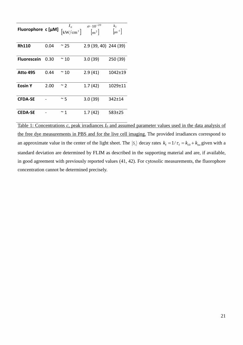
performed in phosphate buffered saline (PBS, pH 7.4). Table 1 presents irradiances and concentrations

used in the measurements of the dyes, together with the photophysical parameters used in the data

analysis, based on own measurements and literature values (39–42).

To establish a focal overlap between the illumination and detection pathways in the SPIM configuration,

the cylindrical lens was taken off to create a symmetrically focused illumination beam. Its shape was

imaged through the detection objective using the fluorescence response of a dye solution. The size of the

illumination beam’s image could then be minimized to co-align the foci of the two objectives.

7

For every dye, 56 different illumination pulse trains with different tp were applied onto the sample.

Generally, was kept constant at 1 % and for the consecutive pulse trains, tp was increased

logarithmically from 100 ns up to 10 ms. The total illumination time, that is the total time within a pulse

train during which the specimen was subject to excitation, was kept constant for all sequences and equal

to the longest tp applied (10 ms). Each pulse within a sequence was considered to be perfectly rectangular,

as previously validated (20).

The AOM does not completely block the light in between the pulses, but approximately 0.2% of the

initial irradiance is transmitted, which artificially increases the counts in an acquired image. This is

corrected for by subtracting a background image from each measurement. Inherent bleaching is

monitored and corrected for by taking a control image with tp set to 100 ns after every fourth pulse train.

These control images are fitted pixel-wise by a single exponential decay, yielding a set of correction

factors for every image.

The focus of the illumination in the propagation direction was obtained by exploiting the fluorescence

depletion in an image of free dye in solution. For CW excitation, the signal in the focus of illumination is

depleted, because this region is subject to higher irradiances, causing an increase in dark state build-up.

The propagation direction of the excitation beam was checked by fitting the intensity distributions along

several vertical lines by Gaussian functions, yielding a center position along each line.

All fitting procedures were performed using a Levenberg-Marquardt algorithm, implemented on a custom

MATLAB 7.11.0 software. In order to obtain sufficient statistics and to reduce calculation time, the

images are resized by binning into pixel sizes of 1x1 μm².

The detection volume in confocal TRAST is estimated by fitting a two-dimensional Gaussian function to

the intensity distribution in a non-depleted fluorescence image. For the used alignment, the e-2

excitation

beam waists in focus were found to be 770 nm and 860 nm.

The recorded SPIM-TRAST curves for Rhodamine 110, Atto 495 and Fluorescein were fitted by Eq. S15,

corresponding to an STR model. For Eosin Y, the analysis was based on the four-state S01TR model (Eq.

1) to account for its large intersystem crossing rate, which renders the simplifications of the STR model

inappropriate. In all cases, the excitation cross section and the 1S decay rates were fixed to the values

provided in table 1 and k01 was calculated using Eq. S20 (see supporting material).

Cell Preparation Protocol for Live Cell SPIM-TRAST Imaging

Michigan cancer foundation cell line 7 (MCF-7) cells were stained with the fluorescein derivative

5-(and-6)-Carboxyfluorescein diacetate succinimidyl ester (CFDA-SE, Life Technologies Corp.,

Carlsbad, USA) or the Eosin derivative 5-(and-6)-Carboxyeosin diacetate succinimidyl ester (CEDA-SE,

Life Technologies Corp.). MCF-7 cells were routinely cultured in DMEM (Dulbecco’s Modified Eagle

8

Medium) or MEM (Minimum Essential Medium, both Life Technologies Corp.) with 10% FBS (Fetal

Bovine Serum, Life Technologies Corp), 0.4% of a 100x non-essential amino acids solution (Sigma

Aldrich, St. Louis, MO, USA) and 1 mM sodium pyruvate (M7145, Sigma Aldrich).

First, the adherent cells grown in a 35 mm Petri dishes were washed twice with 37°C PBS, then incubated

(10 min, at 37 °C, 5% CO2) in the staining solution (either 20 µM CEDA-SE or 3 µM CFDA-SE in

colorless RPMI without FBS). Afterwards, the cells were washed twice in Roswell Park Memorial

Institute medium (RPMI, incl. 10% FBS) and incubated for 30 minutes.

After staining, the adherent cells were washed with PBS and detached from the surface during five

minutes of incubation in 0.5 ml of TrypLE (Life Technologies Corp.). The entire volume was transferred

to a tube and spinned (5 min at 1500 rpm, Centrifuge 5804 R, Eppendorf AG, Hamburg, Germany). The

supernatant was taken off, the cells were dissolved in RPMI (incl. 10% FBS) and the concentration of

cells was estimated in a cell counting device.

A 1.2 w% agarose (Boehringer, Mannheim, Germany) in ddH2O mixture was heated in a microwave (43).

For cell mounting, equal volumes of 1.2 w% agarose, 2×RPMI (prepared from powder form, Life

Technologies Corp) and the prepared stock of stained MCF-7 cells were mixed. This isotonic liquid was

transferred into the sample chamber before it became a gel. Labeled MCF-7 cells were thus randomly

distributed in an agarose gel having a similar refractive index as water (26). To minimize scattering from

cells present in the illumination beam before the focus (30), but to still find sufficient numbers of MCF-7

cells, a concentration of ~2106 cells per milliliter sample volume was found to be a good trade-off.

Live Cell Imaging

The majority of steps for in vivo SPIM-TRAST are similar to solution measurements. In an initial step,

the chamber was loaded with free dye dissolved in agarose and the alignment of illumination and

detection foci was done as described previously for the solution measurements. To reduce bleaching and

photodamage in cell measurements, the maximum pulse widths were set to 1 ms for CEDA-SE staining

and to 0.2 ms for CFDA-SE. The number of applied pulse trains was set to 19 for both dyes and the

chosen excitation irradiances are listed in table 1.

The center of the illumination profile was localized as in the solution measurements, exploiting the low

background fluorescence from phenol red, contained in the medium. For this procedure, the stage was

moved to a region containing no cells and 100× longer illumination times as in cell measurements were

used to detect the background fluorescence.

Since the Zeiss C-Apochromat objective used for cell imaging has a better collection efficiency than the

one used in solution measurements, the images are resized to smaller bins prior to fitting (0.6×0.6 μm²).

The excitation rates were found to be significantly reduced in cell measurements compared to solution

9

measurements. This can be due to the adjustment of the vertical position of the cells, which might result

in a non-perfect overlap between the excitation and detection foci. Moreover, scattering due to cells

present in the illumination pathway can decrease the irradiance and may distort the beam profile. To

correct for both effects, the effective excitation rate was reduced by a factor between 0 and 1 in the

evaluation of the TRAST curves. This reduction factor was determined separately for each cell by an

initial fit over the mean fluorescence TRAST curve averaged over the whole cell of consideration. For

this procedure, we considered only the first part of the TRAST curve corresponding to the triplet state

decay (up to a pulse width of five times the characteristic time of the triplet decay), which was fitted by

Eq. S17. In this fit, the excitation rate, calculated according to Eq. S20, was averaged over the cell and

the intersystem crossing rate remained fixed to 120 µs-1

for CEDA-SE and 10 µs-1

for CFDA-SE. The

measurements on free dye in solution do not demand this step, since scattering is negligible in these

measurements.

In the histograms used to present the results, the bin sizes are set with respect to the Freedman-Diaconis

rule (44), which gives a consistent rule for the binning sizes. The obtained distributions are normalized to

the total number of events and present frequency distributions.

Results and Discussion

Free dye in solution

Transition rates for fluorophores in aqueous solution were determined from data recorded by the SPIM-

TRAST instrument, following the procedures described in the methods and materials section above. The

determined rates were compared to previously published data to validate the overall approach as a tool for

measuring these parameters. To verify the estimation of the excitation, SPIM-TRAST measurements were

performed at several excitation powers (Fig. 2 and S5).

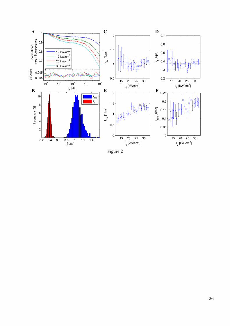
Fig. 2 A shows representative TRAST curves for measurements on Rhodamine 110 at different peak

excitation irradiances, I0. Each of the curves corresponds to the mean over an area of 40×18 μm² around

the center of illumination. Fig. 2 C and D show the intersystem crossing rates, kisc, and the triplet decay

rates, kt, obtained by separately fitting the experimental TRAST curves recorded in each pixel at different

excitations I0 using Eq. S16 (equivalent to Eq. 1, except that it is based on the simpler STR model). The

data points correspond to the mean rates and the error bars to their standard deviations over the

mentioned area. Both kisc and kt are constant within the standard deviations, indicating that the considered

fitting model and the assumed excitation rate distribution are suitable. It is important to achieve

consistent results within the fitting area, to enable local differences in kt within cells to be resolvable in

the in-vivo measurements. Under isotropic conditions, the obtained distributions of kisc and kt values were

found to have standard deviations around 10% of their means, which should make it possible to resolve

10

local differences of kisc and kt of a corresponding size in the cellular measurements. Representative

histograms for both rates at a selected irradiance are depicted in Fig. 2 B. Fig. 2 C and D show that the kisc

and kt values obtained by fitting do not depend on the applied irradiance. Their standard deviation

decreases however for higher irradiances since both the fluorescence brightness and the contrast of the

TRAST curves increase the certainty of the fitting results.

For the transitions into and out of the redox state, an irradiance dependence is discernible in Fig. 2 E and

F. Such an effect may be caused by higher excited states, which have higher probabilities to be populated

at increasing photon densities, and which also show a stronger yield of redox state formation (18). Those

transitions are not accounted for within the applied model and the fitting procedure may therefore yield

increasing kox with higher I0. However, apart from Rhodamine 110, no increase in oxidation rate could be

seen for the other dyes that were tested in this study (see Fig. S5 D,I,N). These dyes were excited at

considerably lower irradiances and therefore the population of higher excited states was less probable.

The exact determination of redox rates for freely diffusing fluorophores would require consideration of

the diffusion term, as discussed in the supplementary part. Absolutely accurate values of kox and kred are

therefore not accessible within the applied fitting model. Nevertheless, as previously shown by

simulations in (23), the model allows relative changes in redox parameters to be followed.

We conducted similar experiments on several organic fluorophores as shown in Fig. S5. The obtained

transition rates are provided in tables 2 and S2. All outcomes for SPIM-TRAST imaging were reproduced

by confocal TRAST measurements and were in good agreement with literature values, when available.

The TRAST curves were acquired starting from pulse widths of 500 ns for Fluorescein and Atto 495 and

700 ns for Rhodamine 110 and Eosin Y, to ensure equilibration between the two singlet states. For Atto

495, a third dark state appears to be populated for pulses longer than 1 ms, which manifests itself in an

additional decay in the TRAST curves. To minimize the effect of the additional transition when applying

the STR model, we analyzed these data sets only up to 1 ms.

Taken together, the results from the solution measurements on several dyes and at many different I0,

indicate that the SPIM-TRAST setup, including the data analysis and the assumptions on the illumination,

provide a suitable approach to access the transition rates between the transient dark states of

fluorophores.

Acquisition with Arbitrary Duty Cycle Pulse Trains

Next, we evaluated under what conditions in the TRAST measurements the assumption is valid, that all

molecules are in their ground state at the onset of an excitation pulse. First, simulations were performed

following an STR model (Eqs. S23- S24), and based on parameter values for Rhodamine 110 (k10 = 243

μs-1

, kisc = 1 μs-1

, kt = 0.4 μs-1

, kox = 1.4 ms-1

, kred = 0.15 ms-1

, σ = 2.910-20

m2 at λ=491 nm excitation

11

wavelength), 2

0 cmkW25I , and illumination profile and CEF as found in the setup

( 2.1NA,μm6.1,μm40 ,0,0 zy , 33.1n , pixel size 10 μm, magnification 49x). The simulations

indicated that the total dark state population at the beginning of each pulse indeed is small at a duty cycle

of 1% (see Fig. S3). This indication was then tested experimentally by SPIM-TRAST measurements on

Rhodamine 110 in aqueous solution, acquired with different duty cycles η (Fig. 3). The experimental

TRAST curves were then analyzed based on the electronic state model in Fig. S1, now using the solution

to the system of differential equations obtained when no constraints on η are applied, as derived in the

supporting material (Eqs. S23-S24). The intersystem crossing and triplet decay rates obtained based on

this model were found to be in good agreement with the results shown in Fig. 2. As the computational

effort to process the data is considerably higher, a smaller area of 19.5x7.5 μm² and larger pixel sizes

1.5x1.5 μm² were analyzed. The mean rates and standard deviations over this area were determined to

kisc = (1.03±0.07) μs-1

and kt = (0.35±0.01) μs-1

.

From the rate parameters in Fig. 3, no trend is visible between the fitted kisc and kt and the used duty

cycle. These results validate the newly derived model for fitting TRAST data, acquired at arbitrary duty

cycles. Second, this new model makes it possible to decrease measurement times significantly without

loss of precision. The gain in measurement times comes however at the cost of longer analysis times.

Moreover, it can be inferred from these results that the previously used approach is suitable for low duty

cycles.

The rates related to the redox state reveal however a dependence on the duty cycle. For this, different

causes are conceivable. In particular, the contrast in the TRAST curves decreases with increasing duty

cycle, causing less certainty in the outcome. Moreover, as the duty cycle increases, the pause between

two pulses, which allows for fluorophore recovery, decreases. As discussed in the previous section, we

can, with the model used in this work, only expect to be able to follow relative changes in the redox rates.

However, these relative changes can be well reflected in the obtained fitting results, independent of the

applied duty cycle.

Live Cell SPIM-TRAST Imaging

The SPIM-TRAST images on MCF-7 cells were analyzed in a different manner from the solution data.

First, the excitation rate was determined by a global fit, as described in the Materials and Methods

section. Then, the TRAST measurements on cells were fitted in a pixel-wise manner using the S01TR

model (Eq. 1) for CEDA-SE and the STR model (Eq. S15) for CFDA-SE. As in previous works (22), the

amount of free parameters was decreased in order to obtain a robust fit at the decreased signal-to-noise

ratio (SNR) experienced in live cell imaging. For the Eosin derivate CEDA-SE, we assumed kisc=120 μs-1

and kred=0.01 ms-1

, and kept kt and kox as free parameters. The chosen kisc value showed the best overall

12

agreement between experimental data and the fits. As the whole decay of R cannot be followed in the

TRAST curves within the maximally applicable pulse widths, kred was fixed to a low boundary in order to

increase the stability of the fitting procedure. The lower kisc of CEDA-SE when bound to proteins, as

compared to Eosin Y in solution, can be explained by O2 shielding effects and viscosity changes of the

protein environment. Fluorescence lifetime imaging microscopy (FLIM) also yields faster fluorescence

decay rates (10 isc1 f k k ) for Eosin Y, as compared to protein bound CEDA-SE, as summarized in table

1. This further supports the view that kisc is indeed higher for Eosin Y in solution. Although the assumed

rates may introduce a bias in the fitted kt and kox values, the capability of imaging relative changes

between different measurement conditions or local differences within a cell is maintained. The same

arguments hold for CFDA-SE, for which we assumed kisc=10 μs-1

and kred=0.05 ms-1

.

A representative MCF-7 cell stained with CEDA-SE is depicted in Fig. 4. An almost homogeneous

labeling could be achieved, as seen in the fluorescence intensity image in Fig. 4 A. The TRAST curves

acquired in each of the pixels representing the cell were fitted separately, as described in the paragraph

above. Fig. 4 D shows the average fluorescence TRAST curve and the average of the fit applied to each

pixel over the pixels of the MCF-7 cell in Fig. 4 A. The residuals were found to be slightly larger than in

the solution measurements, which could be due to small cell movements, or the fixed rates possibly

deviating from the real values. However, the TRAST curve approaches the measurement data properly,

and allows for the spatially resolved determination of kt as shown in Fig. 4 B. The average and standard

deviation of kt over the pixels of the cell in Fig. 4 B read 1t ms2.100.91 k . In Fig. 4B, the kt image

shows gradients, with faster rates being measured in the cell center, a feature we found for practically all

the measured cells. No obvious spatial relation between the fluorescence image and the obtained kt-image

can be noticed, indicating that the kt-image does not seem to be biased by the local fluorescence intensity

levels. Instead, the kt rates can be expected to be proportional to the concentration of molecular oxygen,

which is a predominant triplet state quencher (17). The found kt rate distribution in the cells thus rather

indicates a depletion of oxygen in the periphery of the cell.

In contrast, the kox-images (Fig. 4 C) revealed patterns much more influenced by noise. This is partly a

result of that the maximum pulse width was shorter than the full redox decay in the TRAST curves.

Moreover, due to the large triplet yield, CEDA-SE mainly populates its triplet state upon excitation, and

thus has its strengths primarily for the investigation of triplet states. The mean rate and the standard

deviation over the cell in the kox image in Fig. 4 D was determined to 1ox ms2.04.0 k .

To distinguish between reasonably fitted and noise governed outcomes, the starting value of kox in the

fitting procedure of the experimental data was set to values below the detectable limit (1 s-1

). After fitting,

a distinct peak in the distribution of kox could be well separated from the lower threshold, and all

13

determined oxidation rates, which were equal or lower than this starting value, were disregarded. In Fig.

S6 A, a histogram of the determined kox values and their 95% confidence intervals is shown, as

determined in 88 measurements on 21 different cells. From this histogram, it is clear that for the

disregarded pixel values falling below the threshold, the confidence intervals are significantly larger. This

further justifies the omission of these values from subsequent analyses.

In Fig. 4E, the obtained rates from the 399 pixels comprising the image of the cell are displayed in a kox-kt

2D-histogram. The obtained kt distribution in Fig 4E is broader than in the case of solution measurements

(Fig. 2) where a comparable amount of pixels is considered. As a clear spatial pattern is obtained in the kt

images, not related to the local fluorescence intensity levels, the main reason for the broadening of the kt

distribution is likely the heterogeneous intracellular environment and oxygen depletion. Moreover, the

kox-kt 2D-histogram reveals an inclination, indicating a correlation between the fitted kt and kox values.

To further investigate these findings, we compiled a corresponding 2D-histogram from 88 measurements

on 21 different cells, comprising a total of 40590 pixels (Fig. S6 B). This histogram includes data from

measurements on different days since the day-to-day variation was small compared to the intrinsic

spread. The kt- and the kox-distributions show distinct peaks. Their means and standard deviations were

found to be: 1

t ms7.195.92 k and 1

ox ms3.05.0 k . Again, the distribution of the triplet decay

rates is broader than that from the solution measurements.

Concerning the kox-distribution, both the intracellular distributions in reducing and oxidating agents, and

the limited observable tp range of the redox decay in the TRAST curves can be possible reasons for the

large spread of kox-values. Nevertheless, the distribution reveals a distinct peak and thus a relative, mean

oxidation rate. SPIM-TRAST measurements thus provide a relative measure for the detection of the

redox state of investigated cells, potentially to be used e.g. to screen potentially toxic substances and their

influence on cellular redox levels.

The inclination of the 2D-histograms for CEDA-SE in Fig. 4E is seen also in the histogram presented in

Fig. S6 B, representing the compiled results for many cells. The inclination could at least partly be due

the fact that both values are not estimated independently. Another possible reason for the correlation

between kox and kt could be the oxygen concentration, since oxygen can enhance both triplet state decay

rates and oxidation rates of fluorophores (18). The tilted ellipse may thus be a manifestation of different

local oxygen concentrations in the cells.

Similarly, we also performed measurements on MCF-7 cells, using the Fluorescein derivative CFDA-SE

(Fig. 5 A-D). The previous discussion for CEDA-SE is also valid for CFDA-SE. However, the applied

irradiance, the determined rates and hence the dark state build-up are different. The following mean and

standard deviations were obtained from the pixel values of the cell presented in Fig. 5:

1

t ms9.145.179 k and 1

ox ms9.00.5 k . Compared to CEDA-SE, the Fluorescein derivate is

14

better suited for imaging kox. Although its high bleaching rate does not allow using illumination schemes

with pulse widths over 200 μs, a larger part of the redox process is still visible in the curves, since the

rates are significantly faster. Therefore in general only very few pixels had to be omitted for reasons of

non-convergence to a reasonable solution (as described above for CEDA-SE).

Similar to the results on CEDA-SE, the 2D-histograms indicate a slight correlation between the kt and kox

rates (Fig. 5E). The same holds, when the results from 27 measurements on 13 different MCF-7 cells are

taken together, as shown in Fig. S6 C. Both the triplet decay and the oxidation rates appear to be

distributed around central, unique peaks, with the following means and standard deviations:

1

t ms3.479.180 k and 1

ox ms0.33.5 k . The anticipated reason for the broadness of the

distributions is also in this case the heterogeneous intracellular environment. Moreover, Fluorescein is

known to have a strongly pH-dependent brightness (45, 46) and the corresponding protonation-

deprotonation reactions may therefore also partly contribute to the broadening.

Conclusions

We have demonstrated a novel combination of Transient State (TRAST) imaging and Single Plane

Illumination Microscopy (SPIM). By this concept, the overall excitation light exposure of the specimen

can be considerably reduced. Transition rates of free dye in solution were found to be determined

accurately, and imaging of oxygen gradients, as well as relative oxidation rates in live cells was

demonstrated. A new theoretical framework was derived, and validated by simulations and experiments,

which allows the analysis of TRAST data, acquired with arbitrary duty cycle pulse trains. This approach

makes it possible to increase the obtainable frame rates of TRAST imaging by more than a factor of 10

compared to previous experiments. Taken together, these developments reduce the constraints further and

extend the applicability of TRAST imaging for live cells studies.

Supporting material

Derivations, simulations, supporting figures, tables and equations are available at

www.biophys.org/biophysj/supplemental/S0006-3495(XX)XXXXX-X.

Acknowledgments

This work was supported by means from EU FP7 (FLUODIAMON 201 837), the Swedish Research

Council (VRNT 2012-3045), and the Knut and Alice Wallenberg Foundation (KAW 2011.0218). T. S.

was supported by the National Research Fund, Luxembourg. The authors thank Thorsten Wohland, Natl

Univ Singapore, for advice regarding the SPIM configuration.

15

Supporting Citations

References (47–53) appear in the Supporting Material.

16

References

1. Donnert, G., J. Keller, R. Medda, M.A. Andrei, S.O. Rizzoli, et al. 2006. Macromolecular-scale

resolution in biological fluorescence microscopy. Proc Natl Acad Sci U S A. 103: 11440–5.

2. Donnert, G., C. Eggeling, and S.W. Hell. 2007. Major signal increase in fluorescence microscopy

through dark-state relaxation. Nat Methods. 4: 81–86.

3. Widengren, J., and R. Rigler. 1996. Mechanisms of photobleaching investigated by fluorescence

correlation spectroscopy. Bioimaging. 4: 149–157.

4. Eggeling, C., J. Widengren, R. Rigler, and C.A.M. Seidel. 1998. Photobleaching of Fluorescent

Dyes under Conditions Used for Single-Molecule Detection: Evidence of Two-Step Photolysis.

Anal Chem. 70: 2651–9.

5. Hell, S.W., and M. Kroug. 1995. Ground-state-depletion fluorscence microscopy: a concept for

breaking the diffraction resolution limit. Appl Phys B. 60: 495–497.

6. Betzig, E., G.H. Patterson, R. Sougrat, O.W. Lindwasser, S. Olenych, et al. 2006. Imaging

intracellular fluorescent proteins at nanometer resolution. Science. 313: 1642–5.

7. Rust, M.J., M. Bates, and X. Zhuang. 2006. Imaging by stochastic optical reconstruction

microscopy (STORM). Nat Methods. 3: 793–795.

8. Widengren, J. 2010. Fluorescence-based transient state monitoring for biomolecular spectroscopy

and imaging. J R Soc Interface. 7: 1135–1144.

9. Korobov, V.E., and A.K. Chibisov. 1978. Primary dyes processes in the photochemistry of

rhodamine. Journal of Photochemistry. 9: 411–424.

10. Chen, E., and M.R. Chance. 1993. Nanosecond transient absorption spectroscopy. Methods

Enzymol. 226: 119–147.

11. Peterman, E.J., F.M. Dukker, R. van Grondelle, and H. van Amerongen. 1995. Chlorophyll a and

carotenoid triplet states in light-harvesting complex II of higher plants. Biophys J. 69: 2670–8.

17

12. Van Amerongen, H., and R. van Grondelle. 1995. Transient absorption spectroscopy in study of

processes and dynamics in biology. Methods Enzymol. 246: 201–26.

13. Vanderkooi, J.M., G. Maniara, T.J. Green, and D.F. Wilson. 1987. An optical method for

measurement of dioxygen concentration based upon quenching of phosphorescence. J Biol Chem.

262: 5476–82.

14. Marriott, G., R.M. Clegg, D.J. Arndt-Jovin, and T.M. Jovin. 1991. Time resolved imaging

microscopy Phosphorescence and delayed fluorescence imaging. Biophys J. 60: 1374–1387.

15. Dunphy, I., S.A. Vinogradov, and D.F. Wilson. 2002. Oxyphor R2 and G2: phosphors for

measuring oxygen by oxygen-dependent quenching of phosphorescence. Anal Biochem. 310: 191–

8.

16. Widengren, J., R. Rigler, and Ü. Mets. 1994. Triplet-State Monitoring by Fluorescence Correlation

Spectroscopy. Medical Biochemistry. 4: 3–6.

17. Widengren, J., Ü. Mets, and R. Rigler. 1995. Fluorescence correlation spectroscopy of triplet states

in solution: a theoretical and experimental study. J Phys Chem. 99: 13368–13379.

18. Widengren, J., and P. Schwille. 2000. Characterization of Photoinduced Isomerization and Back-

Isomerization of the Cyanine Dye Cy5 by Fluorescence Correlation Spectroscopy. J Phys Chem A.

104: 6416–6428.

19. Widengren, J., A. Chmyrov, C. Eggeling, P.-A. Löfdahl, and C.A.M. Seidel. 2007. Strategies to

improve photostabilities in ultrasensitive fluorescence spectroscopy. J Phys Chem A. 111: 429–40.

20. Sandén, T., G. Persson, P. Thyberg, H. Blom, and J. Widengren. 2007. Monitoring kinetics of

highly environment sensitive states of fluorescent molecules by modulated excitation and time-

averaged fluorescence intensity recording. Anal Chem. 79: 3330–41.

21. Sandén, T., G. Persson, and J. Widengren. 2008. Transient state imaging for microenvironmental

monitoring by laser scanning microscopy. Anal Chem. 80: 9589–96.

22. Geissbuehler, M., T. Spielmann, A. Formey, I. Märki, M. Leutenegger, et al. 2010. Triplet imaging

of oxygen consumption during the contraction of a single smooth muscle cell (A7r5). Biophys J.

98: 339–49.

18

23. Spielmann, T., H. Blom, M. Geissbuehler, T. Lasser, and J. Widengren. 2010. Transient state

monitoring by total internal reflection fluorescence microscopy. J Phys Chem B. 114: 4035–46.

24. Wagner, M., P. Weber, T. Bruns, W.S.L. Strauss, R. Wittig, et al. 2010. Light dose is a limiting

factor to maintain cell viability in fluorescence microscopy and single molecule detection. Int J

Mol Sci. 11: 956–66.

25. Huisken, J., and D.Y.R. Stainier. 2009. Selective plane illumination microscopy techniques in

developmental biology. Development. 136: 1963–75.

26. Huisken, J., J. Swoger, F. Del Bene, J. Wittbrodt, and E.H.K. Stelzer. 2004. Optical sectioning

deep inside live embryos by selective plane illumination microscopy. Science. 305: 1007–1009.

27. Ritter, J.G., R. Veith, J.-P. Siebrasse, and U. Kubitscheck. 2008. High-contrast single-particle

tracking by selective focal plane illumination microscopy. Opt Express. 16: 7142–52.

28. Voie, A.H., D.H. Burns, and F.A. Spelman. 1993. Orthogonal-plane fluorescence optical

sectioning: three-dimensional imaging of macroscopic biological specimens. Journal of

Microscopy. 170: 229–236.

29. Engelbrecht, C.J., and E.H. Stelzer. 2006. Resolution enhancement in a light-sheet-based

microscope (SPIM). Opt Lett. 31: 1477–9.

30. Zanacchi, F.C., Z. Lavagnino, M.P. Donnorso, A. Del Bue, L. Furia, et al. 2011. Live-cell 3D

super-resolution imaging in thick biological samples. Nat Methods. 8: 1047–1050.

31. Keller, P.J., A.D. Schmidt, A. Santella, K. Khairy, Z. Bao, et al. 2010. Fast, high-contrast imaging

of animal development with scanned light sheet-based structured-illumination microscopy. Nat

Methods. 7: 637–42.

32. Wohland, T., X. Shi, J. Sankaran, and E.H.K. Stelzer. 2010. Single plane illumination fluorescence

correlation spectroscopy (SPIM-FCS) probes inhomogeneous three-dimensional environments.

Opt Express. 18: 10627–41.

33. Buchholz, J., J.W. Krieger, G. Mocsáe, B. Kreith, E. Charbon, et al. 2011. FPGA implementation

of a 32x32 autocorrelator array for analysis of fast image series. arXiv. 1112.1619v.

19

34. Buchholz, J., J.W. Krieger, A. Pernus, E. Charbon, U. Kebschull, et al. 2012. Dual-Color Single

Plane Illumination Fluorescence Correlation Spectroscopy (SPIM-FCS) using a Single Photon

Detector and Hardware Based Image Processing. Biophys J. 102: 207a.

35. Chmyrov, A., T. Sandén, and J. Widengren. 2010. Iodide as a fluorescence quencher and promoter

- mechanisms and possible implications. J Phys Chem B. 114: 11282–91.

36. Stein, I., S. Capone, J.H. Smit, F. Baumann, T. Cordes, et al. 2011. Linking Single-Molecule

Blinking to Chromophore Structure and Redox Potentials. ChemPhysChem. 13: 931–937.

37. Greger, K., J. Swoger, and E.H.K. Stelzer. 2007. Basic building units and properties of a

fluorescence single plane illumination microscope. Review of Scientific Instruments. 78: 023705.

38. Saleh, B.E.A., and C.T. Teich. 1991. Fundamentals of Photonics. John Wiley & Sons.

39. Blom, H., A. Chmyrov, K. Hassler, L.M. Davis, and J. Widengren. 2009. Triplet-state

investigations of fluorescent dyes at dielectric interfaces using total internal reflection fluorescence

correlation spectroscopy. J Phys Chem A. 113: 5554–66.

40. Life Technologies. Spectrum Rhodamine 110.

http://probes.invitrogen.com/media/spectra/data/6479ph7.txt Accessed 20/09/12. .

41. ATTO-TEC. Atto 495. https://www.atto-tec.com/

attotecshop/print_product_info.php?products_id=100&XTCsid=h9376va9q25bt3gslh98qipll2

Accessed 20/09/12. .

42. Reindl, S., and A. Penzkofer. 1996. Triplet quantum yield determination by picosecond laser

double-pulse fluorescence excitation. Chem Phys. 213: 429–438.

43. Gault, C. 2010. Soft Agar Colony Formation Assay.

http://www.musc.edu/BCMB/faculty/HOLab/Protocols/files/Soft_Agar_Colony_Formation_Assay

_for_Group.pdf Accessed 27/09/12. .

44. Freedman, D., and P. Diaconis. 1981. On the histogram as a density estimator:L 2 theory.

Zeitschrift für Wahrscheinlichkeitstheorie und Verwandte Gebiete. 57: 453–476.

45. Brändén, M., T. Sandén, P. Brzezinski, and J. Widengren. 2006. Localized proton microcircuits at

the biological membrane-water interface. Proc Natl Acad Sci U S A. 103: 19766–70.

20

46. Sandén, T., L. Salomonsson, P. Brzezinski, and J. Widengren. 2010. Surface-coupled proton

exchange of a membrane-bound proton acceptor. Proc Natl Acad Sci U S A. 107: 4129–34.

47. Beaumont, P.C., D.G. Johnson, and B.J. Parsons. 1993. Photophysical properties of laser dyes:

picosecond laser flash photolysis studies of Rhodamine 6G, Rhodamine B and Rhodamine 101.

Journal of the Chemical Society, Faraday Transactions. 89: 4185.

48. Penzkofer, A., and A. Beidoun. 1993. Triplet-triplet absorption of eosin Y in methanol determined

by nanosecond excimer laser excitation and picosecond light continuum probing. Chem Phys. 177:

203–216.

49. Cohen-Tannoudji, C., B. Diu, and F. Laloë. 1997. Quantum Mechanics. Wiley-Interscience.

50. Ambrose, W.P., T. Basche, and W.E. Moerner. 1991. Detection and spectroscopy of single

pentacene molecules in a p-terphenyl crystal by means of fluorescence excitation. The Journal of

Chemical Physics. 95: 7150.

51. Visscher, K., G.J. Brakenhoff, and T.D. Visser. 1994. Fluorescence Saturation in Optical

Microscopy. J Microsc. 175: 3479.

52. Arya, S.K., K.C. Lee, D. Bin Dah’alan, Daniel, and A.R.A. Rahman. 2012. Breast tumor cell

detection at single cell resolution using an electrochemical impedance technique. Lab Chip. 12:

2362–8.

53. Suhling, K., J. Siegel, P.M.P. Lanigan, S. Lévêque-Fort, S.E.D. Webb, et al. 2004. Time-resolved

fluorescence anisotropy imaging applied to live cells. Opt Lett. 29: 584–586.

21

Fluorophore c [μM] 2

0

cmkW

I 2

20

m

10 1

f

μs -

k

Rh110 0.04 ~ 25 2.9 (39, 40) 244 (39)

Fluorescein 0.30 ~ 10 3.0 (39) 250 (39)

Atto 495 0.44 ~ 10 2.9 (41) 1042±19

Eosin Y 2.00 ~ 2 1.7 (42) 1029±11

CFDA-SE - ~ 5 3.0 (39) 342±14

CEDA-SE - ~ 1 1.7 (42) 583±25

Table 1: Concentrations c, peak irradiances I0 and assumed parameter values used in the data analysis of

the free dye measurements in PBS and for the live cell imaging. The provided irradiances correspond to

an approximate value in the center of the light sheet. The 1S decay rates isc10ff /1 kkk given with a

standard deviation are determined by FLIM as described in the supporting material and are, if available,

in good agreement with previously reported values (41, 42). For cytosolic measurements, the fluorophore

concentration cannot be determined precisely.

22

kisc [μs-1

] kt [μs-1

]

Rh110 SPIM-TRAST 1.05±0.11 0.37±0.04

Conf TRAST 1.18±0.06 0.33±0.02

Reference 1.3±0.1 (39)

1.0±0.1 (39)

1.2±0.2 (23)

0.49±0.03 (39)

0.45±0.04 (39)

0.37±0.02 (23)

Fluorescein SPIM-TRAST 9.29±0.55 0.58±0.03

Conf TRAST 10.30±0.60 0.42±0.03

Reference 13.5±1.0 (39)

11.1±1.0 (39)

0.66±0.04 (39)

0.45±0.04 (39)

Atto 495 SPIM-TRAST 33.64±4.06 1.12±0.13

Conf TRAST 36.43±2.39 0.95±0.05

Eosin Y SPIM-TRAST 746±34 0.48±0.01

Conf TRAST 757±79 0.42±0.02

Reference 420±50 (42)

840±80 (48)

Table 2: Triplet transition rates for Rhodamine 110 (Rh110), Fluorescein, Atto 495 and Eosin Y in PBS

(pH 7.4). The measurements were performed in SPIM-TRAST (720 pixels) and confocal (Conf) TRAST

mode (12 measurements). All error bars correspond to the standard deviations. If found, reference values

are provided. The cited values for Fluorescein were measured in Tris buffer (pH 8.2), whereas the

TRAST measured have been performed in PBS at pH 7.4. However, for both solvents, the majority of

Fluorescein molecules is expected to be deprotonated.

23

Figure titles and legends

Figure 1: Setup and measurement principle for SPIM-TRAST imaging.

A pulse train is created by an AOM from the emission of a CW laser. The use of a cylindrical lens results

in a sheet-like excitation profile in the sample. The fluorophores in the sample can be described by a

simplified, electronic four-state model, comprising two singlet, one triplet and one redox state. The

detection takes place perpendicularly to the excitation sheet and the image is focused and detected on an

EMCCD chip. For each pulse train, with a certain width of the pulses, tp, one image, representing the total

acquired fluorescence, is detected. When plotting this signal as a function of tp, as used in the excitation

schemes, a TRAST curve (bottom left) is obtained in each and every pixel. The acquired points are

subsequently fitted using Eq. 1 or S15, depending on the considered electronic state model, and Eqs. S19-

S20.

Figure 2: TRAST measurement data from free Rhodamine 110 in solution, recorded at different excitation

irradiances.

I0 indicates peak irradiances used in the measurements. Excitation modulation duty cycle of all

measurements: 1%. (A): Representative TRAST curves (+) showing the normalized average fluorescence

intensity over a rectangle of 40x18 pixels, each 1x1 µm² large, and the variation of this intensity with the

excitation pulse width. For every I0, each of the pixels is fitted according to Eqs. S15 and S19-S20 and

the obtained average fitting curves (-) approximate well the measurement data as the residuals appear to

be randomly distributed and do not reveal any systematic deviations. (C, D, E, F): From every fitted

TRAST measurement, a set of four rates is extracted from the TRAST curve of every pixel and the

averages and standard deviations of the rates within the mentioned region is shown. The measurements

were taken for several powers, with the peak irradience I0 in the center of excitation ranging from

2

0 cmkW11I to 2

0 cmkW33I (for clarity not all of these measurements were shown as TRAST

curves in (A)). All standard deviations for kisc and kt over the 720 pixels are around 10% of their means,

or lower. (B) A representative histogram for a measurement at 2

0 cmkW24I is provided, showing

distinct peaks in the distributions of kisc and kt.

24

Figure 3: Data from TRAST measurements on free Rhodamine 110 in solution, acquired with different

duty cycles, η, of the excitation pulse trains.

Excitation irradiance used in the measuremenhts: 2

0 cmkW33I . All values depicted in the TRAST

curves of (A) correspond to the mean fluorescence averaged over a 65 pixels large area, each of them

1.5x1.5 µm² big. The TRAST curves were fitted pixel-wise according to the newly derived model (Eqs.

S22-S24). The residuals indicate that the model accurately represents the measurement data. (B, C, D, E):

The mean and standard deviations of the determined rate parameters within the mentioned region are

shown for each of the TRAST curves in (A), recorded at different η of the excitation pulse trains. The fits

yield consistent results for intersystem crossing (B) and triplet decay rates (C), independent of the length

of the interval between the pulses within each excitation scheme. Their means are in good agreement with

the simplified model (Fig. 2). The obtained redox rates (D and E) however, reveal a slight dependence on

.

Figure 4: Representative measurement on a CEDA-SE stained MCF-7 cell.

The excitation was performed by the previously characterized light sheet at a peak irradiance

2

0 cmkW8.0I and all fits are based on a S01TR model (Eq. 1). (A) shows the fluorescence image of the

cell, (B) the kt-image and (C) the kox-image. All scale bars correspond to 8 µm. (D): The acquired average

TRAST curve (blue) over the whole cell is adequately fitted by the proposed model (red). (E): The 2D-

histogram of the kt and kox values from (B) and (C).

Figure 5: Representative measurement on a CFDA-SE stained MCF-7 cell.

Representative fluorescence image (A), kt-image (B) and kox-image (C) recorded at 2

0 μmkW9.8I and

fitted pixel-wise with a STR model (Eq. S16) (scale bar 8 µm). (D): The acquired mean TRAST (blue)

and fitted (red) curve averaged over the whole are in good agreement. (E): The 2D-histogram of the kt

and kox values presented in (B) and (C).

25

Figures

Figure 1

26

Figure 2

27

Figure 3

28

Figure 4

Figure 5

1

Supporting Material

Electronic State Model

The S01TR model of Fig. 1 includes some simplifications, as summarized below. In the model, only oxidations originating from the triplet state are considered, although such transitions can also occur from excited singlet states (1). Since the redox- rates kox and kred are

much slower than all the other rates of the S01TR model, 0S , 1S and T are after onset of

excitation usually equilibrated well before population and equilibration of R has taken

place. For e.g. organic dyes in air-saturated aqueous solution, redox state build-up typically equilibrates in the range of milliseconds after onset of excitation, much later than the triplet formation, which is usually equilibrated within microseconds (2, 3). In the S01TR model, the

photoinduced formation rates of R , from 1S , and from T , thereby differ only by a

scaling factor, which justifies considering oxidations only to originate from the triplet state (4).

Higher excited singlet and triplet states are disregarded in the model, because the corresponding excitation cross section is for conventional organic dyes smaller than the cross section from the ground to the first excited singlet state (5), and such higher excited states usually decay orders of magnitude faster, within picoseconds (6).

Moreover, for any sample with a spatial extension, the excitation rate, k01, depends on the spatial position as defined by the illumination profile and has in case of pulsed excitation also a temporal dependence. For the sake of simplicity, the spatial dependence of k01 is not denoted explicitly in the following. The same holds for kisc, kt, kox and kred, which also may have spatial dependencies in non-homogenous samples. Regarding the temporal dependence of k01, rectangular excitation pulse trains are used in this study, with time-independent excitation rates within the pulses.

The probabilities of populating the four different states of a fluorophore, described by the S01TR model of Fig 1, and with the fluorophore subject to an excitation pulse with constant k01, can be derived from the general form of a set of first order differential equations.

)()(dd

tSMtSt

rr= ,

(S1)

where the state vector Sr

and the transition matrix M take the form:

−−−

−−−

=

=

redox

oxtisc

isc1001

redt1001

1

0

00

00

00,

)(

)(

)(

)(

0101

kk

kkk

kkk

kkkk

tR

tT

tS

tS

S TRSTRS Mr

(S2)

For the majority of organic dyes, k01 and the de-excitation rate, k10, are orders of magnitude faster than the triplet-related transition rates. The introduced model can then be simplified by unifying both singlet states, as they are equilibrated before any significant triplet state build-

2

up occurs (Fig. S1). The system is then reduced to a three-state STR model. Such an

assumption requires the introduction of an effective intersystem crossing rate isck ′ , which

corresponds to the product of the actual intersystem crossing and the 1S population at

equilibrium (3) :

1001

01iscisc k+k

kk=k′ (S3)

For a STR model Eq. S2 simplifies to:

−′′−

=

=

redox

oxtisc

redtisc

0

0--,

)(

)(

)(

kk

kkk

kkk

tR

tT

tS

S STRSTR Mr

(S4)

For both the S01TR and the STR model, the sum of all elements of Sr

are assumed to be conserved and equal to 1 for all times. This assumption presumes constant concentrations and hence no photo-bleaching. Although photo-bleaching is present to some extent in our experiments, it can be properly corrected for, and the assumption is therefore still valid.

It should be noted that the assumptions namely tisc1001 ,, kkkk >> , made for introducing the

STR model, is applicable for a wide range of organic dyes, but does not hold for the rates found for Eosin Y. Thus, this fluorophore’s dynamics have to be approached using the S01TR model.

Sets of differential equations like Eq. S1 have been solved before (3, 4, 7). A unique solution of the set of differential equations can only be found for a given initial condition. Often, only

0S is assumed to be populated at the time t0=0. Here, a general solution is derived by

introducing a propagator ),( 0ttU , which, based on an initial state )( 0tSr

, maps the

corresponding vector at time t (8).

Figure S1: The simplified Jablonski diagram for a four-state model (Fig. 1) can be narrowed down to a three-level system if at onset of excitation both singlet states are equilibrated before the transient dark states are populated to a noteworthy extent.

3

∫ ′′=

=t

t

ttttU

tStttS

0

)d)(exp(),(

)(),()(

0

00

M

Urr

(S5)

The propagator, ),( 0ttU , is thus a matrix exponential and the integral can be evaluated

trivially as long as M is time-independent. Since the exponential of a diagonal matrix consists simply of the exponentials of the diagonal elements, a transfer to the eigenspace of M is

useful. Both, TRS01M and STRM are diagonalizable. We define P as the eigenvector matrix of

M , containing in the i-th column the eigenvector ivr and Λ as the corresponding eigenvalue

matrix having as diagonal elements the eigenvalues iλ of M : ijiijδλ=Λ .

Under these conditions the propagator can be found using the projection matrix P to the

eigenspace and its inverse 1−P . The inverse projection exists in every case, as P consists of linearly independent basis vectors. Hence, its determinant cannot be equal to zero.

( ) 100 )(exp),( −−= PΛPU tttt

(S6)

From now on, the solution will be applied to the STR model, but the solution to S01TR

follows an analogous derivation. The projection of STRM into the eigenspace reads:

+′+′′++′++′′

+++++=

)()(

))(())((

)()()(

3iscox2iscoxoxisc

3red3isc2red2iscredisc

oxtred3toxtred2toxtred

λλλλλλ

λλ

kkkkkk

kkkkkk

kkkkkkkkkkk

P (S7)

P is based on the following eigenvalues λi:

)(4)(2

1

2

0

oxiscredoxredtredisc2

redoxtiscredoxtisc

3,2

1

kkkkkkkkkkkkkkkk ′+++′−+++′+++′

−=

=

mλ

λ

(S8)

The first eigenvalue corresponds to the equilibrium situation, while λ2 and λ3 are the inverse characteristic times of triplet and redox equilibration. As long as the eigenvalues are clearly

separated (i.e. 32 λλ >> ), the eigenvalues can be approximated as (4):

( )tisc2 k+k′−=λ and ( )redox3 k+k ′−=λ (S9)

with tisc

iscoxox kk

kkk

+′′

=′ .

When observing fluorescence emission, the evolution of the singlet state population, S(t), is of particular interest. An expression for S(t) upon onset of continuous wave excitation is

accessed by applying the propagator to an initial vector )( 0tSr

. Using the conservation of

probability ttRtTtS ∀−−= ),()(1)( yields:

4

)(0

ox

oxisc2redred03isc

323

2tisc

)(0

ox

oxisc3redred02isc

322

3tisc

32

oxtred

03

02

)()(

)()(

)()(

)()(

)()(

tt

tt

etRk

kkkktTk

kk

etRk

kkkktTk

kkkkktS

−

−

′−+++′

−++′

−

′−+++′

−++′

++

=

λ

λ

λλλλλ

λ

λλλλλ

λλλ

(S10)

When taking [ ] T0 0,0,1)( =tS

ras an initial condition, and considering that redoxtisc ,, kkkk >>′ , a

Taylor series expansion yields a simplified evolution of the singlet state population:

)(

redoxtisc

oxt)(

tisc

isc

redoxtisc

tred 0302

))(())(()( tttt e

kkkk

kke

kk

k

kkkk

kktS −−

+′+′′

++′′

++′+′

= λλ (S11)

As this model assumes an instantaneous equilibration between both singlet states, the fraction

of S, which corresponds to 1S , is obtained by considering the equilibrium conditions of a

hypothetical two-level system:

)()(1001

011 tS

kk

ktS

+= (S12)

Average fluorescence signal upon pulsed excitation schemes of low duty cycle

The emitted fluorescence )(S tF from a fluorophore in the sample is directly proportional to

the population of the excited singlet state:

)()()(1001

0110F110FS tS

kk

kktSktF

+Φ=Φ= (S13)

TRAST imaging is based on integrating the fluorescence over an entire pulse train, consisting of N excitation pulses with constant height, width tp and period time T. The corresponding

duty cycle is defined as T

t p=η . Consequently, the mean signal, that is the total fluorescence

in the sample, averaged over the total exposure time Ntp of one excitation pulse train, reads:

∑ ∫−

=

+

+Φ=

1

01001

0110 )(

1)(

N

j

tjT

jT p

pNt

p

pttS

Ntkk

kktF dFS (S14)

Here k01 can be considered as time-independent, even though the excitation is pulsed. Only the on-state yields a fluorescence response within the STR model. For our rectangular pulse trains with constant height of the excitation pulses, all fluorescence contributing to )( pNtS tF

P

is generated by a constant k01. In case an S01TR model is assumed, there is some fluorescence for a short time after a pulse has ended. This corresponds to the still excited molecules, which emit fluorescence, but are relaxed within nanoseconds after the excitation is turned off. The amount of photons released during this time is small compared to the signal acquired during one pulse, which is always chosen to be at least 100 nanoseconds long, and can thus be neglected. Consequently, all summands in Eq. S14 become equivalent when the time is

5

formally reset to zero after each pulse period, as the initial condition at the onset of each pulse is always identical. This holds if the pause between two pulses is long enough to allow for a complete relaxation of the fluorophore into its ground state. Under these conditions, the mean fluorescence response to a pulse train is obtained from Eq. S11 and S14:

( ) ( )

( )

−

+′+′′

+

−

+′′

++′+′+

Φ=

1))((

1))((

)(

3

2

3

21001

0110

p

p

p

t

p

t

p

pNt

ekkkkt

kk

ekkt

k

kkkk

kk

kk

kktF

λ

λ

λ

λ

redoxtisc

oxisc

tisc

isc

redoxtisc

tredFS

(S15)

To compare Eq. S15 to Eq. 1 in the main article, it can be rewritten using the approximated eigenvalues introduced in Eq. S9.

( ) ( )

+−

′−−

′+

Φ= p

tt

p

pNtt

kke

kke

k

tkk

kktF pp

p32

2

32

2

21001

0110 32 111

)(λλλλλ

λλ tredoxisciscFS (S16)

In this notation, the two models can be seen to be equal for 11 λ>>pt , (as in the main text,

the eigenvalue )( 10011 kk +−=λ , represents from now on the equilibration of the singlet states)

indicating that the STR model is valid as long as all tp–values are larger than the singlet state equilibration time.

The S01T model can be derived from Eq. 1 by considering the case of a S01TR model, where the dark state is much faster depopulated than populated: i.e.: oxred kk ′>>

( ) ( )

−

−

′+−= p

tt

p

pNtt

kk

t

FtF pp

p2

2

21

0 21 e1e11

)(λλλ

λλ tiscS

(S17)

Derivation of the effective excitation rate.

In the TRAST measurements, each pixel on the CCD array, assigned a position (α,β), is detecting the fluorescence originating from a volume centered around a position (xα, yβ) in the sample (from the focal plane of the detection objective 0=z ). The detected fluorescence

),,( tF βαD in a single pixel of the CCD with coordinates (α,β) can be expressed by a two-

dimensional convolution:

zyxzyyxxtzyxFtrctF ddd),,(CEF),,,(),(),,( SDD βαφβα −−= ∫∫∫ (S18)

Here, Dφ is the detection efficiency of the detection path and the CCD and ),( trc denotes the

concentration of fluorophores. FS is given by Eq. S13, and CEF is the collection efficiency function (3). Fluctuations of the dye concentration are neglected (4, 7), since TRAST comprises short pulses, which yield only low photodegradation. Furthermore, bleaching is corrected for separately.

6

For a known excitation rate distribution, the acquired fluorescence signal expected upon a pulse train excitation scheme comprising equally long pulses with large duty cycles can be predicted from Eq. 1 or S11 together with Eq. S18. However, when fitting Eq. S18 to experimental data, the execution of the convolution integral is time consuming as it involves several Fourier transforms and a three-dimensional calculation of the expected fluorescence in the sample. Therefore, the model is scaled down to a two-dimensional system. The

fluorescence ),,( pNttF

pβαS in a hypothetical plane is calculated directly using a two

dimensional effective excitation rate ),,(eff01 ptk βα calculated for each pixel. ),,(eff

01 ptk βα

comprises two effects, the irradiance distribution in the sample as well as the collection efficiency. The coordinate system is chosen as before: the light sheet propagates in +x-direction, is collimated in y, and centered at z=0. The normalized fluorescence signal detected

by a pixel (α,β) on the CCD would then read:

),,(

),,(),,(

pnorm

pNtS

pD tF

tFctF p

βα

βαφβα D= (S19)

Here, ),,( ptF βαnorm is a normalization factor, corresponding to the value of ),,( pNttF

pβαS in

the absence of transitions to T or R (see Eq. S21 below). The fluorescence in the sample

has a spatial distribution, mainly due to the applied illumination profile. In order to account for the collection efficiency in the real system, we define the effective excitation rate as (3):

∫∫∫∫∫∫

−−

−−=

zyxzyyxxtzyxF

zyxzyyxxtzyxFzyxktk

pNtS

pNtS

p

p

p

dddCEF

dddCEFeff

),,(),,,(

),,(),,,(),,(),,(

01

01

βα

βαβα (S20)

In this approach, eff01k is weighted with the fluorescence in the sample. As given by Eq. 1, it

depends on the rates of transition, especially the excitation rate itself. The quality of this model requires a proper choice of these parameters when describing the three-dimensional, theoretical mean fluorescence

pNtSF in the sample. Ideally, it is a Gaussian shaped response,

but fluorescence depletion may distort this profile. At the irradiances used in TRAST, we can

neglect saturation effects caused by excessive 1S build-up (9, 10). As a further

simplification, fluorescence depletion due to dark state build-up may also be neglected when

calculating eff01k . This assumption is equivalent to considering two singlet states, which

equilibrate in the nanosecond range. Since the applied pulses are always much longer than this equilibration time, all excitation schemes w ould be equally affected, and the effective excitation rate becomes pulse width invariant (see Fig. S3 B). However, since TRAST is based on populating dark states, we expected an improvement of the model, by taking non-

fluorescent states into account when calculating eff01k , using the full, pulse width dependent

Eq. 1 for the mean fluorescence distribution in Eq. S20. Within this approach, eff01k decreases

with increasing dark state build-up. This decay of eff01k with increasing pulse width has two

major effects: Firstly, it corrects for fluorescence depletion, which is wanted on purpose.

7

Secondly, it makes pulse trains with different pulse widths incomparable. It has been assumed that longer pulses yield lower average fluorescence rates within the pulses, which is

accounted for by finding an adjusted ),,(eff01 ptk βα . On the other hand, a decreased excitation

rate also causes a drop of the fluorescence, due to a lower build-up of 1S . To correct for this

additional effect, Eq. S19 contains a normalization factor, which is dependent on the excitation scheme, namely its pulse width. In essence, it represents the undepleted fluorescence signal for an assumed excitation rate. The relation, describing this particular

value, is Eq. S14 in the limit 0→pt . Consequently, the expression used for fitting CCD-

based SPIM-TRAST measurements is Eq. S19, with ),,( pnorm tF βα given by:

10eff01

eff01

10F ),,(

),,(),,(

ktk

tkktF

p

ppnorm +

Φ=βα

βαβα (S21)

Simulations on the Effective Excitation Rate

The performance of the approach of Eqs. S19-S21 was further tested by simulations. The simulations were performed for Eosin Y in solution, using the parameters mentioned in Fig S3, and for an area of 40x18 µm2, comprising 1x1 µm² large pixels. The larger side of this rectangle is oriented in parallel to the illumination beam propagation. Its length is chosen with respect to the Rayleigh range of the excitation profile. The shape of the illumination beam is simulated using parameters found in the setup (see Fig. S3). All excitation cross sections and the fluorescence rates are selected with respect to table 1.

Since the calculation of eff01k yields slightly better results when the fluorescence saturation due

to dark states is not disregarded, we decided to base the data analysis in this study on that approach. The derived fitting model is a powerful tool as it simplifies the real system and reduces computational processing. However, it assumes starting values of transition rates in Eq. S20. Since the overall objective is to extract exactly these rates, the initial guesses ought to be close to the real values and the procedure has to be iterated until convergence occurs.

With increasing pulse width of the pulsed excitation scheme in TRAST and thus growing dark state build-up, the fluorescence response to a Gaussian shaped excitation flattens towards a rectangular profile as indicated in Eq. 1 and as shown in Fig. S3A. When calculating the effective excitation rate (Fig. S3 B) for the pixel, which images the center of the light sheet, there is no pulse width dependence, if fluorescence saturation due to dark state build-up is

neglected (blue line). However, with the dark state build-up taken into account, eff01k reveals

the expected pulse width dependent decrease. Although the depicted decrease amounts only to a few percent, its effect still needs to be evaluated.

Fig. S3 C compares both approaches. As a reference, we calculated the convolution integral (Eq. S23) for several pulse widths (+ in Fig. S3 C). Second, we used Eq. S19-21 with and without taking dark state build-up into account. Although the deviations are small, the model which disregards fluorescence saturation due to dark state build-up (blue line) does not fit the simulated data as well, as when the depletion is taken into account (red line).

8

Moreover, it is shown that the normalization factor normF is crucial, as it corrects for the drop

in the calculated fluorescence signal, which accompanies the pulse width dependent decrease

of eff01k . Following the same calculation as above, with depletion taken into account when

calculating eff01k , but omitting the pulse-width dependence of the normalization factor, yields

larger deviations compared to the reference values. For this neglection (green line), the TRAST curve decays too fast compared to the prediction based on Eq. S19.

Apparently, both approaches for eff01k match the prediction from the convolution integral quite

well. However, this is not the prior focus of TRAST imaging. We are rather seeking to extract the transition rates as accurately as possible. To validate both models with respect to this demand, we simulated CCD images of TRAST measurements for the organic dyes

Figure S2: Simulations performed for Eosin Y, assuming typical transition rates (k10 = 329 µs-1, kisc = 700 µs-1, kt = 0.4 µs-1, kox = 1 ms-1, kred = 0.5 ms-1), an excitation cross section σ = 1.7⋅10-20 m2 for λ0=491 nm excitation wavelength and a peak irradiance of

20 µmµW10=I . The illumination profile and the CEF are simulated with parameters as

found in the setup ( ,40,0 my µω = 2.1NA,6.1,0 == mz µω refractive index 33.1n = , pixel size

10 µm, magnification 49x). (A) The fluorescence response to a Gaussian excitation of width 1.6 µm reshapes towards a rectangular profile. This results from fluorescence saturation, which is caused by increasing dark state build-up as the applied pulse width increases. (B) The corresponding, effective excitation rate (-, and * for the particular cases from above) decreases respectively, unless fluorescence saturation is neglected. In this case, eff

01k remains constant for all excitation schemes. (C) Several TRAST curve are

calculated in the different, discussed fashions. We consider the calculation based on the convolution integral (Eq. S20) as the true decay (crosses). Obviously, it is matched best, when eff

01k is calculated without disregarding fluorescence saturation (red). Nevertheless,

even if fluorescence saturation due to dark states is neglected when calculating eff01k , the

obtained curve is still close (blue). If the introduced normalization factor Fnorm is neglected, this deteriorates the outcome by an overestimation of the decay (green).

9

Rhodamine 110, Fluorescein, Atto 495 and Eosin Y. These calculations are based on Eq. S15 and S18. In contrast to all other investigated dyes, the simplified STR model does not hold for Eosin Y. Accordingly, the S01TR (Eq. 1 instead of Eq. S15) is applied in this case.

The simulated results are fitted in two different ways. First, the effective excitation rate is

considered to be the same for all pulse trains ( ),(eff01 βαk ). Its dependence on fluorescence

depletion is neglected. Subsequently, this particular effect is taken into consideration and the

effective excitation rate ( ),,(eff01 ptk βα ) is pulse width dependent. The starting values for kisc,

kt, kox and kred were set 10% off the assumed value, in order to ensure that a convergence occurs within the fitting procedure. The results of these simulations are provided in table S1. Indeed, the approach, which takes the effect of fluorescence depletion into consideration

when calculatingeff01k , yields better results.

In most cases the differences between both models are negligible. In order to show deviations, the values are presented with higher accuracy than it is achievable in actual measurements. Analogous simulations for different irradiances reproduced the assumed values equally well. Even though both fitting procedures yielded sufficiently good results, data processing in this study is performed using the slightly more precise model including fluorescence depletion due to dark state build up.

kisc [µs-1] kt [µs

-1] kox [ms-1] kred [ms-1] Rhodamine 110 assumed 1.00 0.45 1.00 0.20

20 cm

kW35=I

),(01 βαeffk 0.99±0.01 0.46±0.01 0.98±0.01 0.21±0.01

),,(01 ptk βαeff 1.00±0.01 0.45±0.01 1.00±0.01 0.20±0.01

Fluorescein assumed 13.50 0.66 5.00 0.50

20 cmkW

20=I ),(01 βαeffk 13.30±0.02 0.70±0.01 4.62±0.02 0.59±0.01

),,(01 ptk βαeff 13.55±0.01 0.67±0.01 5.00±0.01 0.51±0.01

Atto 495 assumed 30.00 1.00 4.00 2.00

20 cm

kW20=I

),(01 βαeffk 29.94±0.01 1.03±0.01 3.88±0.01 2.08±0.01

),,(01 ptk βαeff 30.01±0.01 1.01±0.01 4.02±0.01 2.01±0.01

Eosin Y assumed 840 0.40 0.60 0.30

20 cm

kW1=I

),(01 βαeffk 836±2 0.42±0.01 0.57±0.01 0.32±0.01

),,(01 ptk βαeff 842±2 0.40±0.01 0.60±0.01 0.30±0.01

Table S1: Assumed and subsequently obtained transition rates of Rhodamine 110, Fluorescein, Atto 495 and Eosin Y. The TRAST curves were simulated with respect to the given values. All obtained results were fitted with two different approaches. Either assuming the same effective excitation rates for all pulse widths ( ),(01 βαeffk ), or taking the effect of

fluorescence depletion into account ( ),,(01 ptk βαeff ).

10

Average fluorescence signal upon application of pulsed excitation schemes of arbitrary duty cycles

As derived in the section above, the theoretical treatment of TRAST data simplifies significantly with low excitation duty cycles (4). However, it may be desired to reduce the acquisition time and thus the pause between pulses. In the following, an adequate model for arbitrary duty cycles is derived, based on the propagation operators introduced in Eq. S5. To calculate the mean fluorescence for one pulse train, the average singlet state population within the pulses needs to be calculated. Any spatial dependence arising from the excitation profile is not considered for the moment. Following Eq. S14, we denote the time-average of S(t) within the excitation pulses as:

∑ ∫−

=

+

=

1

0

)(1

)(N

j

tjT

jT p

pNt

p

pttS

NttS d (S22)

Without loss of generality, the time can be reset to zero after each period. S(t) is given by Eq. S10.The initial triplet and redox populations Tj(0), Rj(0) at the onset of the j-th pulse strongly depend on the length and number of prior pulses, as well as on the pauses in-between them. These initial conditions constitute the only difference between each and every addend in Eq. S22. As the excitation rate is piecewise constant, the integration yields:

p

t

p

t

pNt

t

eR

k

kkkkT

kkk

t

eR

k

kkkkT

kkk

kkktS

p

p

p

1)(

)(

1)(

)(

)()(

3

2

3

2

3323

2

2

3

2322

3

32

−

′−+++′

−++′

−

−

′−+++′

−++′

+

+=

λ

λ

λλ

λλλλλ

λλ

λλλλλ

λλ

initox

oxiscredredinit

isctisc

initox

oxiscredredinit

isctisc

oxtred

(S23)

Interestingly, )( pNttS

p depends on the average initial occupation of both dark states initT ,

initR over all pulses, as defined in Eq. S24. At this point, it becomes beneficial to have time

evolution operators.

No assumptions have been made about isck′ in the derivation so far, except for the physical

demand to be positive semidefinite as all other rates. The case isck′ = 0 has not been excluded.

Consequently, if the excitation is turned off, the eigenvalues and eigenvectors of )0( isc

off =′= kMM and the corresponding propagator offU are obtained directly from U by

setting the effective intersystem crossing rate to 0. As the analytical expression of U is quite long and not of particular interest in the derivation, it is included in the appendix below. For the sake of clarity, the time evolution operators, which describe the dynamics when the excitation is turned on, are denoted as onU in the following. Applying both propagators for excitation turned on and off subsequently to the initial state at the onset of the j-th pulse, yields the corresponding initial population for the following pulse. This allows for turning the calculation of the means of initial populations into a geometric matrix series:

11

( )∑∑−

=

−

=

=

=

1

0

off1

0init

init

init

0

0

1

)0,(),(1

)0(

)0(

)0(1 N

j

j

pon

p

N

jj

j

j

ttTN

R

T

S

NR

T

S

UU (S24)

It has been assumed that at the very first pulse, the fluorophore is in its ground state. Unfortunately, both propagators do not commute, neither is the standard solution of geometric series

( ) [ ] [ ][ ]N

pon

ppon

p

N

j

j

pon

p ttTttTttT )0,(),()0,(),()0,(),( off1off

1

1off UUUUUU −Ε−Ε=−

=

−∑ (S25)

applicable, because as the system tends to equilibrium, the product of both time evolution operators approaches the unity operator E. As an alternative, the numerical determination of

the eigenvalues of [ ])0,(),(offp

onp ttT UU and a subsequent projection into the eigenspace can

save computation time when calculating initT and initR .

If the duty cycle is kept sufficiently small, initT and initR will tend to zero, because the

pause will be long enough to allow full relaxation back into the ground state.

A solution to this kind of problem has been already presented by Sandén et al. (7). However, that approach does not rely on time evolution operators. The benefit of this derivation is the representation in term of matrices, which makes the computational implementation for fitting purposes substantially faster and easier to implement.

12

Simulations on the initial conditions at the onset of a pulse

As described above, the assumption of low duty cycles makes it possible to simplify the data analysis. We compared this simplifying approach with the thorough solution, based on Eqs. S23-S24, including calculations of the fluorescence signal from Rhodamine 110 in solution detected in a single pixel, using Eq. S18 and suitable parameters, as stated in Fig. S3. Firstly, as indicated in Eq. S22-S24, it is of interest to consider the mean of all initial singlet, triplet and redox populations for all pulses of the applied excitation scheme (<Sinit>, <Tinit> and <Rinit>). As shown in Fig. S3 A-C, these populations can only be neglected for excitation pulse trains with low duty cycles η, having long pauses between the pulses. The simulations reveal that <Rinit> is always higher than <Tinit>. This is in agreement with the much slower redox dynamics, compared to the orders of magnitude faster triplet decay.

Figure S3: (A, B, C): The average population at the onset of all pulses depends in a STR model on the applied pulse width and the duty cycle η. The shorter the time between two pulses, the less the assumption of relaxed fluorophores at the onset of a pulse is valid. (D): With increasing duty cycle, the contrast in the TRAST curves decreases. The simplified approach by Spielmann et al. (4) is similar to the thoroughly derived approach in the limit of η→0. For η=0.01, the triplet related decay is still described properly by the simplified model, but deviations occur. These data have been simulated for Rhodamine 110 (k10 = 243 µs-1, kisc = 1 µs-1, kt = 0.4 µs-1, kox = 1.4 ms-1, kred = 0.15 ms-1, σ = 2.9⋅10-20 m2 at λ=491 nm excitation wavelength, peak irradiance 2

0 µmµW25.0=I ), exposed to pulse trains of different pulse widths, but identical total exposure time (Ntp) of 1ms. The illumination profile and the CEF are simulated with parameters as found in the setup (

2.1NA,6.1,40 ,0,0 === mm zy µωµω , refractive index 33.1n = , pixel size 10 µm, magnification

49x).

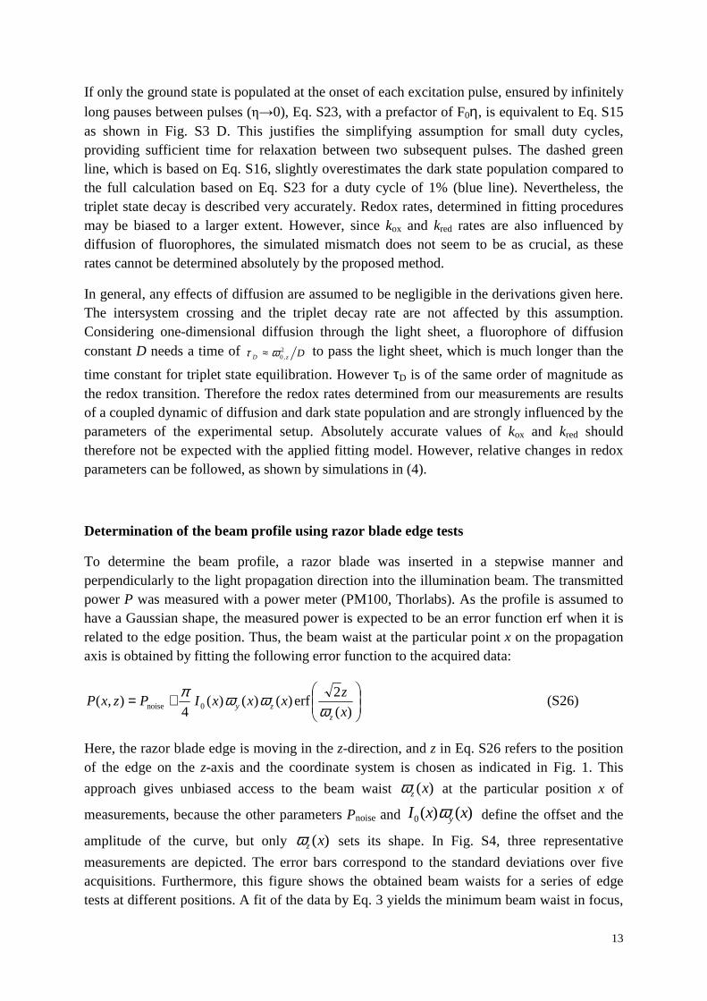
13

If only the ground state is populated at the onset of each excitation pulse, ensured by infinitely

long pauses between pulses (η→0), Eq. S23, with a prefactor of F0η, is equivalent to Eq. S15 as shown in Fig. S3 D. This justifies the simplifying assumption for small duty cycles, providing sufficient time for relaxation between two subsequent pulses. The dashed green line, which is based on Eq. S16, slightly overestimates the dark state population compared to the full calculation based on Eq. S23 for a duty cycle of 1% (blue line). Nevertheless, the triplet state decay is described very accurately. Redox rates, determined in fitting procedures may be biased to a larger extent. However, since kox and kred rates are also influenced by diffusion of fluorophores, the simulated mismatch does not seem to be as crucial, as these rates cannot be determined absolutely by the proposed method.

In general, any effects of diffusion are assumed to be negligible in the derivations given here. The intersystem crossing and the triplet decay rate are not affected by this assumption. Considering one-dimensional diffusion through the light sheet, a fluorophore of diffusion constant D needs a time of DzD

2,0ωτ ≈ to pass the light sheet, which is much longer than the

time constant for triplet state equilibration. However τD is of the same order of magnitude as the redox transition. Therefore the redox rates determined from our measurements are results of a coupled dynamic of diffusion and dark state population and are strongly influenced by the parameters of the experimental setup. Absolutely accurate values of kox and kred should therefore not be expected with the applied fitting model. However, relative changes in redox parameters can be followed, as shown by simulations in (4).

Determination of the beam profile using razor blade edge tests

To determine the beam profile, a razor blade was inserted in a stepwise manner and perpendicularly to the light propagation direction into the illumination beam. The transmitted power P was measured with a power meter (PM100, Thorlabs). As the profile is assumed to have a Gaussian shape, the measured power is expected to be an error function erf when it is related to the edge position. Thus, the beam waist at the particular point x on the propagation axis is obtained by fitting the following error function to the acquired data:

+=

)(

2erf)()()(

4),( 0noise x

zxxxIPzxP

zzy ω

ωωπ (S26)

Here, the razor blade edge is moving in the z-direction, and z in Eq. S26 refers to the position of the edge on the z-axis and the coordinate system is chosen as indicated in Fig. 1. This

approach gives unbiased access to the beam waist )(xzω at the particular position x of

measurements, because the other parameters Pnoise and )()(0 xxI yω define the offset and the

amplitude of the curve, but only )(xzω sets its shape. In Fig. S4, three representative

measurements are depicted. The error bars correspond to the standard deviations over five acquisitions. Furthermore, this figure shows the obtained beam waists for a series of edge tests at different positions. A fit of the data by Eq. 3 yields the minimum beam waist in focus,

14

which is found to be ( )1.06.1,0 ±=zω µm. In this case, the error represents the 95%

confidence interval of the fit. In this particular setup, the light sheet (vacuum wavelength

4910 =λ nm) is focused in water. Thus, the Rayleigh range is ( )7.28.21,R ±=zx µm, which

provides sheet-like illumination conditions within more than 40µm around the center of focus. This width is large enough to perform single cell imaging, as it is performed in this study on MCF-7 cells, which have diameters around 18µm (11). By similar means, the beam waist of

the collimated dimension is found to be 40,0 =yω µm.

The presented razor blade edge tests provide access to the beam waists in the sample, even though they are performed in air. The beam diameter in focus is neither affected by the refractive medium, nor by the interface when entering the sample chamber. The change due to the different focusing angle is accounted for by including the refractive indices into the calculations.

FLIM measurements

Fluorescence lifetime measurements by time-correlated single photon counting were performed with a typical epi-illuminated confocal microscope equipped with stage scanning capabilities. Cell samples were excited with a 476 nm pulsed (repetition rate: 50 MHz) laser ( Becker and Hickl, Berlin Germany in collaboration with LASOS , Jena, Germany) at a power of around 2 µW for cell images and around 20 µW for solution, as measured at the objective

Figure S4: Illumination profile along the light propagation axis x. The beam waist at different positions is determined by several knife edge tests (blue). Each individual point results from fitting an error function to the acquired data (inset). The minimum beam diameter in focus is determined by fitting a Gaussian beam behavior to the data (red).

15

(Olympus UPLANAPO, 60x/1.20w). The excitation beam was guided to an OLYMPUS IX70 (Olympus, Hamburg, Germany) microscope stand in which imaging was performed via a scanning stage (MadCityLabs, Madison, USA). The detection was performed either by two APDs (SPCM AQR-14; PerkinElmer Inc.,Waltham, USA) and/or by two Hybrid PMTs (HPM-100-50; Hamamatsu, Japan). Images (128x128 pixels) over a field of view of 43 µm were obtained. The data sets were analyzed by a software package developed by the group of C. A. M. Seidel, Heinrich-Heine Univ, Düsseldorf (http://www.mpc.uni-duesseldorf.de/seidel/index.htm). The experimental fluorescence decay curves, recorded for each pixel and deconvoluted with respect to the laser pulse duration, were fitted to a single exponential decay model.

The fluorescence lifetimes of Atto 495 and Eosin Y were determined in a PBS buffer droplet on the cover glass. The error deviations represent the standard deviations of at least 3 consecutive measurements.

For determination of the fluorescence lifetime of CFDA-SE and CEDA-SE within labeled MCF-7 cells, three cells stained with each dye were measured on the setup described above. For these measurements, the cells were grown on chambered cover glasses and freshly labeled according to labeling steps described in the cell preparation steps in the main text. During these measurements cells were at room temperature and in air atmosphere. Homogenous lifetime images were obtained similar to the one seen in (12). The mean and the standard deviation of the mean lifetimes averaged over three individual cells is given in table 1.

16

Figure S5: SPIM-TRAST measurements on Eosin Y (A-E), Atto 495 (F-J) and Fluorescein (K-P).

17

Figure S6: (A): The 2D histogram showing the kox distribution on the y-axis and their

uncertainty (95% confidence intervals) on the x-axis. This histogram includes the pixel-values

from 88 measurements on 21 different cells, stained with CEDA-SE. The values below a

threshold of 1 s-1

have large uncertainties, which justifies their omission from the histograms,

thereby distinguishing between reasonably fitted and noise governed outcomes. All compiled

measurements were taken at the same peak irradiance (2

0 cmkW8.0=I ). (B): The 2D-

histogram of the kt and kox values of the same measurements as in (A) reveals an inclination

with respect to the axes, which may be a hint for a correlation between the parameters. For

this graph, the pixels with kox values below the aforementioned threshold were rejected. (C)

The 2D histogram of kt and kox values, obtained from 27 measurements on 13 different cells

stained with CFDA-SE. As for CEDA-SE, this figure reveals an inclination with respect to the

axes. Moreover, there may be a subpopulation discernible in the graph, as the distribution is

not centered, but has its maximum on the lower border of the two-dimensional histogram. All

measurements of the CFDA-SE stained cells were taken with a peak excitation irradiance

20 cmkW9.8=I .

18

kox [ms-1] kred [ms-1] Rhodamine 110 SPIM-TRAST 1.1±0.3 0.2±0.1 Confocal TRAST 1.7±0.3 1.1±0.3 Fluorescein SPIM-TRAST 4.0±0.3 0.3±0.1 Confocal TRAST 3.4±0.2 1.4±0.1 Atto 495 SPIM-TRAST 4.4±0.7 1.6±0.6 Confocal TRAST 4.7±0.3 2.4±0.3 Eosin Y SPIM-TRAST 0.9±0.1 0.5±0.1 Confocal TRAST 1.2±0.2 1.2±0.3 Table S2: Redox transition rates for Rhodamine 110, Fluorescein, Atto 495 and Eosin Y in PBS. The values refer to the same measurements as tab. 2. They are not universal values, but rather represent diffusion and redox build-up, which cannot be separated within the conducted analysis.

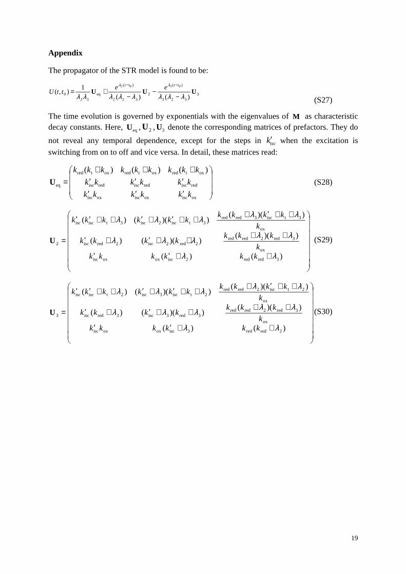
19

Appendix

The propagator of the STR model is found to be:

3323

)(

2322

)(

eq32

0 )()(

1),(

0302

UUUλλλλλλλλ

λλ

−−

−+=

−− tttt eettU

(S27)

The time evolution is governed by exponentials with the eigenvalues of M as characteristic decay constants. Here, eqU , 2U , 3U denote the corresponding matrices of prefactors. They do

not reveal any temporal dependence, except for the steps in isck′ when the excitation is

switching from on to off and vice versa. In detail, these matrices read:

′′′′′′

+++=

oxiscoxiscoxisc

rediscrediscredisc

oxtredoxtredoxtred

eq

)()()(

kkkkkk

kkkkkk

kkkkkkkkk

U (S28)

++′′

++++′+′

++′+++′+′++′′

=

)()(

))(())(()(

))(())(()(

3redred2iscoxoxisc

ox

3red2redred2red2isc2redisc

ox

3tisc3redred3tisc2isc3tiscisc

2

λλ

λλλλλ

λλλλλ

kkkkkkk

kkkkkkk

k

kkkkkkkkkk

U (S29)

++′′

++++′+′

++′+++′+′++′′

=

)()(

))(())(()(

))(())(()(

2redred3iscoxoxisc

ox

3red2redred3red3isc3redisc

ox

2tisc2redred2tisc3isc2tiscisc

3

λλ

λλλλλ

λλλλλ

kkkkkkk

kkkkkkk

k

kkkkkkkkkk

U (S30)

20

Supporting References

1. Widengren, J., A. Chmyrov, C. Eggeling, P.-A. Löfdahl, and C.A.M. Seidel. 2007. Strategies to improve photostabilities in ultrasensitive fluorescence spectroscopy. J Phys Chem A. 111: 429–40.

2. Widengren, J., R. Rigler, and Ü. Mets. 1994. Triplet-State Monitoring by Fluorescence Correlation Spectroscopy. Medical Biochemistry. 4: 3–6.

3. Widengren, J., Ü. Mets, and R. Rigler. 1995. Fluorescence correlation spectroscopy of triplet states in solution: a theoretical and experimental study. J Phys Chem. 99: 13368–13379.

4. Spielmann, T., H. Blom, M. Geissbuehler, T. Lasser, and J. Widengren. 2010. Transient state monitoring by total internal reflection fluorescence microscopy. J Phys Chem B. 114: 4035–46.

5. Beaumont, P.C., D.G. Johnson, and B.J. Parsons. 1993. Photophysical properties of laser dyes: picosecond laser flash photolysis studies of Rhodamine 6G, Rhodamine B and Rhodamine 101. Journal of the Chemical Society, Faraday Transactions. 89: 4185.

6. Penzkofer, A., and A. Beidoun. 1993. Triplet-triplet absorption of eosin Y in methanol determined by nanosecond excimer laser excitation and picosecond light continuum probing. Chem Phys. 177: 203–216.

7. Sandén, T., G. Persson, P. Thyberg, H. Blom, and J. Widengren. 2007. Monitoring kinetics of highly environment sensitive states of fluorescent molecules by modulated excitation and time-averaged fluorescence intensity recording. Anal Chem. 79: 3330–41.

8. Cohen-Tannoudji, C., B. Diu, and F. Laloë. 1997. Quantum Mechanics. Wiley-Interscience.

9. Ambrose, W.P., T. Basché, and W.E. Moerner. 1991. Detection and spectroscopy of single pentacene molecules in a p-terphenyl crystal by means of fluorescence excitation. The Journal of Chemical Physics. 95: 7150.

10. Visscher, K., G.J. Brakenhoff, and T.D. Visser. 1994. Fluorescence Saturation in Optical Microscopy. J Microsc. 175: 3479.

11. Arya, S.K., K.C. Lee, D. Bin Dah’alan, Daniel, and A.R.A. Rahman. 2012. Breast tumor cell detection at single cell resolution using an electrochemical impedance technique. Lab Chip. 12: 2362–8.

12. Suhling, K., J. Siegel, P.M.P. Lanigan, S. Lévêque-Fort, S.E.D. Webb, et al. 2004. Time-resolved fluorescence anisotropy imaging applied to live cells. Opt Lett. 29: 584–586.