MTAEA Multivariable Calculus - Scott McCracken · 2019-11-18 · Multivariable Calculus Geometric...

Multivariable Calculus

MTAEA – Multivariable Calculus

Scott McCracken

School of Economics,Australian National University

February 10, 2010

Scott McCracken MTAEA – Multivariable Calculus


Geometric Representation of Functions.

I When we study functions from R to R, we find it useful tovisualize functions by drawing their graphs.

I When we are concerned with functions of two variables, i.e. fromR2 to R this technique is even more useful.

I As we needed two dimensions to draw the graph of a functionfrom R to R, we need three dimensions to draw the graph of afunction from R2 to R.

I When drawing graphs of unfamiliar functions from R to R in twodimensions, we could mark out a number of points to get an ideaof what the function looks like.

I When we have a function from R2 to R, we can do the same, butbecause of the extra dimension, we need a lot more points tobuild up a graph of the function.



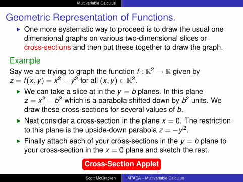
Geometric Representation of Functions.I One more systematic way to proceed is to draw the usual one

dimensional graphs on various two-dimensional slices orcross-sections and then put these together to draw the graph.

ExampleSay we are trying to graph the function f : R2 → R given byz = f (x , y) = x2 − y2 for all (x , y) ∈ R2.

I We can take a slice at in the y = b planes. In this planez = x2 − b2 which is a parabola shifted down by b2 units. Wedraw these cross-sections for several values of b.

I Next consider a cross-section in the plane x = 0. The restrictionto this plane is the upside-down parabola z = −y2.

I Finally attach each of your cross-sections in the y = b plane toyour cross-section in the x = 0 plane and sketch the rest.

Cross-Section Applet


http://www.slu.edu/classes/maymk/banchoff/CrossSection.html


Geometric Representation of Functions.I Another way to visualize a function from R2 to R is to use level

curves. This technique only requires two-dimensional sketching.I For each (x , y) we evaluate f (x , y) to obtain, say b. Then we

draw the locus of points (x , y) in the xy -plane for which f has thesame value b.

Definition.Let f : Rn → R be a function and let b ∈ R. A level set is a set of theform

{(x1, . . . , xn) ∈ Rn | f (x1, . . . , xn) = b}.

I When n = 2,we call a level set a level curve, when n = 3 we callit a level surface and when n ≥ 3. In general we may also call alevel set a level hypersurface. N



Geometric Representation of Functions.ExampleConsider the function given by f (x , y) = x2 − y2.

I Start with the point (0,0) at which f takes value 0. Now find allpoints where f is 0. This is the set {(x , y) | x2 − y2 = 0}, which issimply the inverse image of the set {0} i.e. f ∗(0). This level curveis the set of all points for which x2 = y2 i.e. such that x = ±y .

I Now consider the point (2,1) at which f takes a value of 3. Thelevel curve in this case is

f ∗(3) = {(x , y) | x2 − y2 = 3},

which is a hyperbola centred on the origin with asymptotes y = xand y = −x and focal points

√3 and −

√3.

I Compute more level sets for different b, say −9, −5, −3, 5 and 9.Draw them in the xy -plane and then think of “pulling” each levelcurve up into the z = b plane.




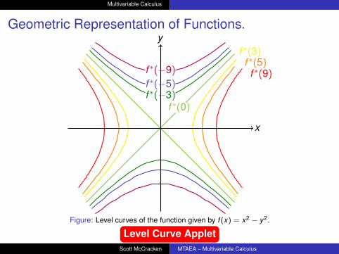
f ∗(−9)

f ∗(−5)f ∗(−3)

f ∗(0)

f ∗(3)f ∗(5)f ∗(9)

x

y

Figure: Level curves of the function given by f (x) = x2 − y2.

Level Curve AppletScott McCracken MTAEA – Multivariable Calculus

http://www.slu.edu/classes/maymk/banchoff/LevelCurve.html



ExampleLevel sets are common in economics.

I An indifference curve is just a level curve of the utility function.Consider a utility function u : R2 → R given by u(x , y). Then forany two bundles (x1, y1) and (x2, y2) on the same level curve theconsumer is indifferent, because u(x1, y1) = u(x2, y2).

I An isoquant is a level curve of a production function. Take asimple Cobb-Douglas production function given by Q = KL,where K and L are quantities of inputs, say captial and labourand Q is the amount output produced from the inputs.

I To draw an isoquant for Q = 10, solve the equation KL = 10 for Lin terms of K and then graph the result. Solving we find that theisoquant for Q = 10 is a branch of a hyperbola L = 10/K .

I Do this for several values of Q, to build up a picture of theproduction function.




I So far we have looked at drawing graphs for functions from R orR2 to R.

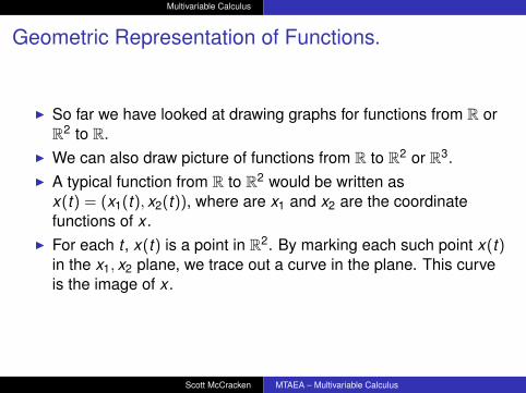
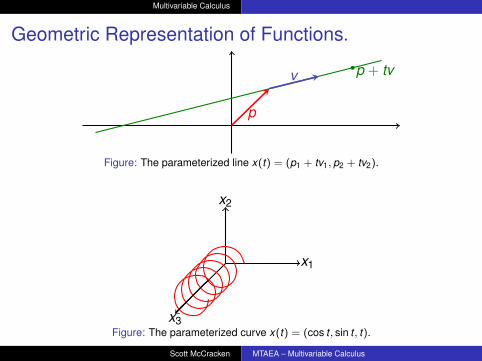
I We can also draw picture of functions from R to R2 or R3.I A typical function from R to R2 would be written as

x(t) = (x1(t), x2(t)), where are x1 and x2 are the coordinatefunctions of x .

I For each t , x(t) is a point in R2. By marking each such point x(t)in the x1, x2 plane, we trace out a curve in the plane. This curveis the image of x .




p + tvv

p

Figure: The parameterized line x(t) = (p1 + tv1, p2 + tv2).

x1

x2

x3Figure: The parameterized curve x(t) = (cos t , sin t , t).



Special Kinds of Functions.Definition.A linear function from Rk to Rm is a function f that preserves thevector space structure, i.e.

f (x + y) = f (x) + f (y) and f (λx) = λf (x)

for all x , y ∈ Rk and all λ ∈ R. Linear functions are sometimes calledlinear transformations. N

ExampleAn example of a linear function is the function f : Rk → R given by

f (x) = a · x = a1x1 + · · ·+ akxk ,

for some a ∈ Rk . �

I It turns out that every linear real-valued function is of the formgiven in the example above.



Special Kinds of Functions.TheoremLet f : Rk → R be a linear function. Then, there exists a vector a ∈ Rk

such that f (x) = a · x for all x ∈ Rk .

I Thus every real-valued function on Rk can be written as

f (x) = a · x =(

a1 · · · ak) x1

...xk

.

I The level sets of a linear function into R are the sets a · x = bwhich we called hyperplanes when we were looking at vectors.

TheoremLet f : Rk → Rm be a linear function. Then, there exists an m × kmatrix A such that f (x) = Ax for all x ∈ Rk .

I This says there that every linear function from Rk to Rm can beassociated with an m × k matrix A.



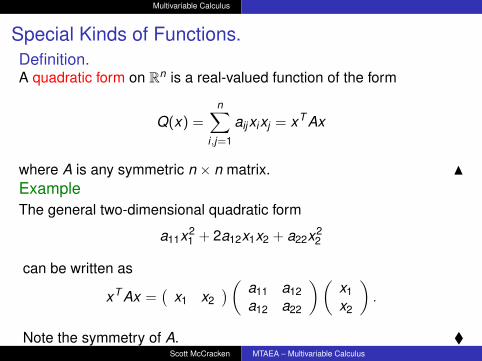
Special Kinds of Functions.Definition.A quadratic form on Rn is a real-valued function of the form

Q(x) =n∑

i,j=1

aijxixj = xT Ax

where A is any symmetric n × n matrix. NExampleThe general two-dimensional quadratic form

a11x21 + 2a12x1x2 + a22x2

2

can be written as

xT Ax =(

x1 x2)( a11 a12

a12 a22

)(x1x2

).

Note the symmetry of A. �Scott McCracken MTAEA – Multivariable Calculus


Special Kinds of Functions.I Linear functions and quadratic forms are special forms of class

of functions called polynomials which are functions made up ofthe sum of monomials.

Definition.A function f : Rk → R is called a monomial if it is of the form

f (x) = cxa11 xa2

2 · · · xakk

where c ∈ R and a1, . . . ,ak are nonnegative integers. The sum of theexponents a1 + · · ·+ ak is called the degree of the monomial. N

Example

(1) f (x1, x2) = −6x31 x2 is a monomial of degree four.

(2) g(x1, x2, x3) = 2x1x2x33 is a monomial of degree five.

(3) A constant function is a monomial of degree zero. �



Special Kinds of Functions.

Definition.A function f : Rk → R is called a polynomial if it is a finite sum ofmonomials on Rk . The highest degree of these monomials is calledthe degree of the polynomial. A function f : Rk → Rm is called apolynomial if each of its coordinate functions is a real-valuedpolynomial. N

Example

(1) f (x1, x2, x3) = 2x21 x3

3 − 5x1x2x43 + 7x8

2 x3 is a polynomial of degreenine.

(2) A linear real-valued function is a polynomial of degree one.(3) A quadratic form is a polynomial of degree two. �



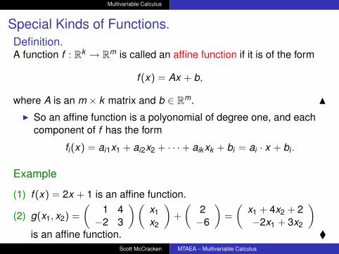
Special Kinds of Functions.Definition.A function f : Rk → Rm is called an affine function if it is of the form

f (x) = Ax + b,

where A is an m × k matrix and b ∈ Rm. N

I So an affine function is a polyonomial of degree one, and eachcomponent of f has the form

fi(x) = ai1x1 + ai2x2 + · · ·+ aikxk + bi = ai · x + bi .

Example

(1) f (x) = 2x + 1 is an affine function.

(2) g(x1, x2) =

(1 4−2 3

)(x1x2

)+

(2−6

)=

(x1 + 4x2 + 2−2x1 + 3x2

)is an affine function. �



Continuous Functions.

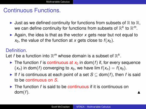
I Just as we defined continuity for functions from subsets of R to R,we can define continuity for functions from subsets of Rk to Rm.

I Again, the idea is that as the vector x gets near but not equal tox0, the value of the function at x gets close to f (x0).

Definition.Let f be a function into Rm whose domain is a subset of Rk .

I The function f is continuous at x0 in dom(f ) if, for every sequence(xn) in dom(f ) converging to x0, we have lim f (xn) = f (x0).

I If f is continuous at each point of a set S ⊆ dom(f ), then f is saidto be continuous on S.

I The function f is said to be continuous if it is continuous ondom(f ). N



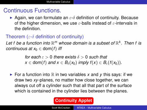
Continuous Functions.I Again, we can formulate an ε-δ definition of continuity. Because

of the higher dimension, we use ε-balls instead of ε-intervals inthe definition.

Theorem (ε-δ definition of continuity)Let f be a function into Rm whose domain is a subset of Rk . Then f iscontinuous at x0 ∈ dom(f ) iff

for each ε > 0 there exists δ > 0 such thatx ∈ dom(f ) and x ∈ Bδ(x0) imply f (x) ∈ Bε(f (x0)).

I For a function into R in two variables x and y this says: if wedraw two xy -planes, no matter how close together, we canalways cut off a cylinder such that all that part of the surfacewhich is contained in the cylinder lies between the planes.

Continuity AppletScott McCracken MTAEA – Multivariable Calculus

http://www.slu.edu/classes/maymk/banchoff/Continuity.html


Continuous Functions.Definition.Let f ,g : Rk → Rm be functions and let c ∈ R. We define newfunctions from Rk into Rm as follows.

I cf given by (cf )(x) = cf (x) = (cf1(x), . . . , cfm(x));I f + g given by (f + g)(x) = (f1(x) + g1(x), . . . , fm(x) + gm(x));I fg given by (fg)(x) = (f1(x)g1(x), . . . , fm(x)gm(x));

for all x ∈ Rk . N

TheoremLet f ,g : Rk → Rm be functions that are continuous at x0 ∈ Rk and letc ∈ R. Then

(i) cf is continuous at x0;

(ii) f + g is continuous at x0;(iii) fg is continuous at x0.



Continuous Functions.

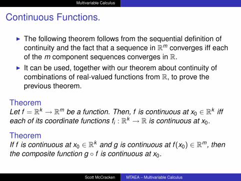
I The following theorem follows from the sequential definition ofcontinuity and the fact that a sequence in Rm converges iff eachof the m component sequences converges in R.

I It can be used, together with our theorem about continuity ofcombinations of real-valued functions from R, to prove theprevious theorem.

TheoremLet f = Rk → Rm be a function. Then, f is continuous at x0 ∈ Rk iffeach of its coordinate functions fi : Rk → R is continuous at x0.

TheoremIf f is continuous at x0 ∈ Rk and g is continuous at f (x0) ∈ Rm, thenthe composite function g ◦ f is continuous at x0.



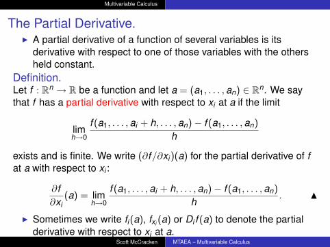
The Partial Derivative.I A partial derivative of a function of several variables is its

derivative with respect to one of those variables with the othersheld constant.

Definition.Let f : Rn → R be a function and let a = (a1, . . . ,an) ∈ Rn. We saythat f has a partial derivative with respect to xi at a if the limit

limh→0

f (a1, . . . ,ai + h, . . . ,an)− f (a1, . . . ,an)

h

exists and is finite. We write (∂f/∂xi)(a) for the partial derivative of fat a with respect to xi :

∂f∂xi

(a) = limh→0

f (a1, . . . ,ai + h, . . . ,an)− f (a1, . . . ,an)

h. N

I Sometimes we write fi(a), fxi (a) or Di f (a) to denote the partialderivative with respect to xi at a.



The Partial Derivative.ExampleConsider the function f given by f (x , y) = 3x3 + 2x2y − 2xy2.

Partial Derivatives Applet


http://www.slu.edu/classes/maymk/banchoff/PartialDerivatives.html


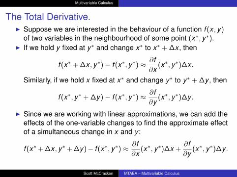
The Total Derivative.I Suppose we are interested in the behaviour of a function f (x , y)

of two variables in the neighbourhood of some point (x∗, y∗).I If we hold y fixed at y∗ and change x∗ to x∗ + ∆x , then

f (x∗ + ∆x , y∗)− f (x∗, y∗) ≈ ∂f∂x

(x∗, y∗)∆x .

Similarly, if we hold x fixed at x∗ and change y∗ to y∗ + ∆y , then

f (x∗, y∗ + ∆y)− f (x∗, y∗) ≈ ∂f∂y

(x∗, y∗)∆y .

I Since we are working with linear approximations, we can add theeffects of the one-variable changes to find the approximate effectof a simultaneous change in x and y :

f (x∗+ ∆x , y∗+ ∆y)− f (x∗, y∗) ≈ ∂f∂x

(x∗, y∗)∆x +∂f∂y

(x∗, y∗)∆y .



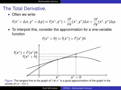
The Total Derivative.I Often we write

f (x∗+ ∆x , y∗+ ∆y) ≈ f (x∗, y∗) +∂f∂x

(x∗, y∗)∆x +∂f∂y

(x∗, y∗)∆y .

I To interpret this, consider the approximation for a one-variablefunction

f (x∗ + h) ≈ f (x∗) + f ′(x∗)h.

f (x∗) + f ′(x∗)h

x∗ + h

f (x∗ + h)

x∗Figure: The tangent line to the graph of f at x∗ is a good approximation of the graph in thevicinity of (x∗, f (x∗).



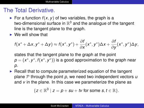
The Total Derivative.I For a function f (x , y) of two variables, the graph is a

two-dimensional surface in R3 and the analogue of the tangentline is the tangent plane to the graph.

I We will show that

f (x∗+ ∆x , y∗+ ∆y) ≈ f (x∗, y∗) +∂f∂x

(x∗, y∗)∆x +∂f∂y

(x∗, y∗)∆y ,

states that the tangent plane to the graph at the pointp = (x∗, y∗, f (x∗, y∗)) is a good approximation to the graph nearp.

I Recall that to compute parameterized equation of the tangentplane P through the point p, we need two independent vectors uand v in the plane. In this case we parameterize the plane as

{z ∈ R3 | z = p + su + tv for some s, t ∈ R}.



The Total Derivative.I u = (1,0, ∂f/∂x(x∗, y∗)) and v = (0,1, ∂f/∂y(x∗, y∗)) are two

independent vectors in the tangent plane.

y

z

x

pu v

x = x∗ y

zp

v

1∂f∂y (x∗, y∗)

y = y∗ x

zp

u

1∂f∂x (x∗, y∗)

Figure: The tangent plane to the graph of f at p = (x∗, y∗) is a good approximation ofthe graph in the vicinity of (x∗, y∗, f (x∗)).

Tangent Plane Applet


http://www.slu.edu/classes/maymk/banchoff/LocalLinearity3d.html


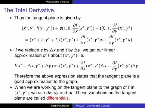
The Total Derivative.I Thus the tangent plane is given by

(x∗, y∗, f (x∗, y∗)) + s(1,0,∂f∂x

(x∗, y∗)) + t(0,1,∂f∂y

(x∗, y∗)

= (x∗ + s, y∗ + t , f (x∗, y∗) +∂f∂x

(x∗, y∗)s +∂f∂y

(x∗, y∗)t)

I If we replace s by ∆x and t by ∆y , we get our linearapproximation of f about (x∗, y∗) i.e.

f (x∗+ ∆x , y∗+ ∆y) ≈ f (x∗, y∗) +∂f∂x

(x∗, y∗)∆x +∂f∂y

(x∗, y∗)∆y .

Therefore the above expression states that the tangent plane is agood approximation to the graph.

I When we are working on the tangent plane to the graph of f at(x∗, y∗), we use dx , dy and df . These variations on the tangentplane are called differentials.



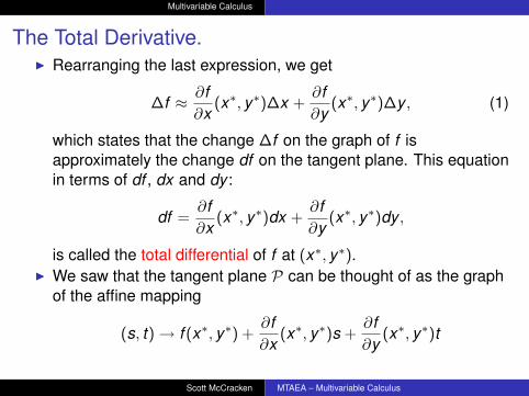
The Total Derivative.I Rearranging the last expression, we get

∆f ≈ ∂f∂x

(x∗, y∗)∆x +∂f∂y

(x∗, y∗)∆y , (1)

which states that the change ∆f on the graph of f isapproximately the change df on the tangent plane. This equationin terms of df , dx and dy :

df =∂f∂x

(x∗, y∗)dx +∂f∂y

(x∗, y∗)dy ,

is called the total differential of f at (x∗, y∗).I We saw that the tangent plane P can be thought of as the graph

of the affine mapping

(s, t)→ f (x∗, y∗) +∂f∂x

(x∗, y∗)s +∂f∂y

(x∗, y∗)t



The Total Derivative.I Thus (1) says the change ∆f can be approximated by the linear

mapping

(s, t)→ ∂f∂x

(x∗, y∗)s +∂f∂y

(x∗, y∗)t ,

which we can write in matrix form as(∂f∂x (x∗, y∗) ∂f

∂y (x∗, y∗))( s

t

).

I Thus we consider the matrix(∂f∂x (x∗, y∗) ∂f

∂y (x∗, y∗)).

as representing the linear approximation of f around (x∗, y∗). Wecall this matrix, or the linear map it represents, the (Jacobian)derivative of f at (x∗, y∗) and denote it as Df (x∗, y∗) or Df(x∗,y∗).



The Total Derivative.

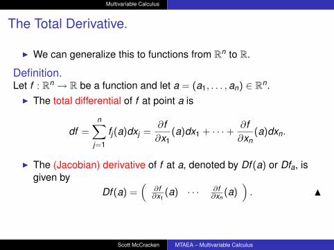
I We can generalize this to functions from Rn to R.

Definition.Let f : Rn → R be a function and let a = (a1, . . . ,an) ∈ Rn.

I The total differential of f at point a is

df =n∑

j=1

fj(a)dxj =∂f∂x1

(a)dx1 + · · ·+ ∂f∂xn

(a)dxn.

I The (Jacobian) derivative of f at a, denoted by Df (a) or Dfa, isgiven by

Df (a) =(

∂f∂x1

(a) · · · ∂f∂xn

(a)). N



The Total Derivative.

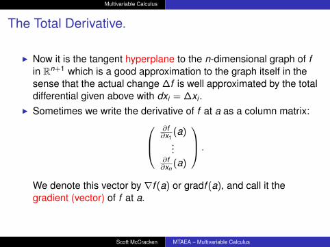
I Now it is the tangent hyperplane to the n-dimensional graph of fin Rn+1 which is a good approximation to the graph itself in thesense that the actual change ∆f is well approximated by the totaldifferential given above with dxi = ∆xi .

I Sometimes we write the derivative of f at a as a column matrix:∂f∂x1

(a)...

∂f∂xn

(a)

.

We denote this vector by ∇f (a) or gradf (a), and call it thegradient (vector) of f at a.



The Chain Rule.I Sometimes we are interested in how a function changes along a

curve in its domain.I For instance, if inputs are changing with time, we may want to

know how the corresponding outputs are changing with time.

Definition.A curve in Rn is a function x : R→ Rn given by

x(t) = (x1(t), . . . , xn(t)),

for all t ∈ R, where each xi : R→ R is a continuous function. Thefunctions xi(t) are called coordinate functions and t is the parameterdescribing the curve. N

I The function x(t) describes the coordinates of the curve at thepoint where the parameter is t .

I If we think of t as time, then x(t) gives the position of a point onits trajectory in Rn at time t .



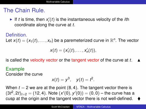
The Chain Rule.I If t is time, then x ′i (t) is the instantaneous velocity of the i th

coordinate along the curve at t .

Definition.Let x(t) = (x1(t), . . . , xn) be a paremeterized curve in Rn. The vector

x(t) = (x ′1(t), . . . , x ′n(t)),

is called the velocity vector or the tangent vector of the curve at t . N

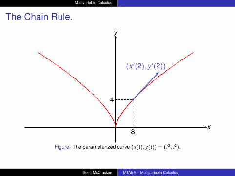
ExampleConsider the curve

x(t) = y3, y(t) = t2.

When t = 2 we are at the point (8,4). The tangent vector there is(3t2,2t)t=2 = (12,4). Note (x ′(0), y ′(0)) = (0,0) – the curve has acusp at the origin and the tangent vector there is not well-defined. �



The Chain Rule.

x

y

8

4

(x ′(2), y ′(2))

Figure: The parameterized curve (x(t), y(t)) = (t3, t2).



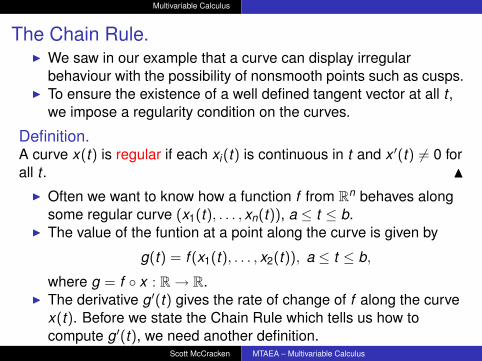
The Chain Rule.I We saw in our example that a curve can display irregular

behaviour with the possibility of nonsmooth points such as cusps.I To ensure the existence of a well defined tangent vector at all t ,

we impose a regularity condition on the curves.

Definition.A curve x(t) is regular if each xi(t) is continuous in t and x ′(t) 6= 0 forall t . N

I Often we want to know how a function f from Rn behaves alongsome regular curve (x1(t), . . . , xn(t)), a ≤ t ≤ b.

I The value of the funtion at a point along the curve is given by

g(t) = f (x1(t), . . . , x2(t)), a ≤ t ≤ b,

where g = f ◦ x : R→ R.I The derivative g′(t) gives the rate of change of f along the curve

x(t). Before we state the Chain Rule which tells us how tocompute g′(t), we need another definition.



The Chain Rule.Definition.

I Let U be an open subset of Rn and let f : Rn → R be a function.We say f is continuously differentiable or C1 on U if all its partialderivatives (∂f/∂xi)(a) exist and are continuous for all a ∈ U.

I A curve x from an open interval into Rn is continuouslydifferentiable (or C1) if each coordinate function xi iscontinuously differentiable. N

Theorem (Chain Rule I)Let x(t) = (x1(t), . . . , xn(t)) be a C1 curve on an open interval abouta and let f : Rn → R be a C1 function on an open ball about x(a).Then g = f ◦ x is a C1 function at a and

dgdt

(a) =dfdt

(x(a)) =∂f∂x1

(x(a))x ′1(a) + · · ·+ ∂f∂xn

(x(a))x ′n(a).



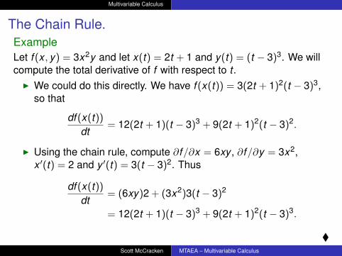
The Chain Rule.ExampleLet f (x , y) = 3x2y and let x(t) = 2t + 1 and y(t) = (t − 3)3. We willcompute the total derivative of f with respect to t .

I We could do this directly. We have f (x(t)) = 3(2t + 1)2(t − 3)3,so that

df (x(t))

dt= 12(2t + 1)(t − 3)3 + 9(2t + 1)2(t − 3)2.

I Using the chain rule, compute ∂f/∂x = 6xy , ∂f/∂y = 3x2,x ′(t) = 2 and y ′(t) = 3(t − 3)2. Thus

df (x(t))

dt= (6xy)2 + (3x2)3(t − 3)2

= 12(2t + 1)(t − 3)3 + 9(2t + 1)2(t − 3)3.

�Scott McCracken MTAEA – Multivariable Calculus


The Chain Rule.

I It is important to distinguish between the total derivative and thepartial derivative.

I Consider a funtion f of three variables x , y , and z.I Usually we assume these variables are independent, but

sometimes they may be dependent on each other – y and z, say,could be functions of x .

I In such cases the partial derivative of f with respect to x doesnot give the true rate of change of f with respect to x , as it doesnot take account of the dependency of y and z on x .

I The total derivative takes these dependencies into account.



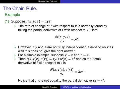
The Chain Rule.Example

(1) Suppose f (x , y , z) = xyz.I The rate of change of f with respect to x is normally found by

taking the partial derivative of f with respect to x . Here

∂f (x , y , z)

∂x= yz.

I However, if y and z are not truly independent but depend on x aswell this does not give the right answer.

I For a simple example, suppose y = x and z = x .I Then f (x , y(x), z(x)) = xy(x)z(x) = x3 and so the (total)

derivative of f with respect to x is

df (x , y(x), z(x))

dx= 3x2.

Notice that this is not equal to the partial derivative yz = x2.



The Chain Rule.(2) Consider the volume of a cone, which depends on the cone’s

height h and radius r according to the formula

V (r ,h) =πr2h

3.

I The partial derivative of V with respect to r is

∂V∂r

=2πrh

3.

It describes the rate with which the cone’s volume changes if itsradius is varied and its height is kept constant.

I The partial derivate with respect to h is

∂V∂h

=πr2

3,

and represents the rate at which the cone’s volume changes if itsheight is changed and its radius kept constant.



The Chain Rule.I Now suppose that r(h), or that h(r). Then the total derivatives with

respect to r or h are

dVdr

=∂V∂r

+∂V∂h

dhdr

dVdh

=∂V∂h

+∂V∂r

drdh

=2πrh

3+πr2

3dhdr

=πr2

3+

2πrh3

drdh.

I The difference between the total and partial derivatives is theignorance of indirect dependencies in the latter.

I If, for some reason, the cone’s proportions have to stay the samewith height and radius in a fixed ratio k , we have

k =hr

=dhdr

I Thus, the total derivative with respect to r is

dVdr

=2πrh

3+ k

πr2

3= kπr2.

�



The Chain Rule.I Sometimes we write the chain rule as

dfdt

=∂f∂x1

dx1

dt+ · · ·+ ∂f

∂xn

dx1

dt.

Compare this with the total differential.I We can generalize the chain rule to the case where the inside

function depends on several variables.

Theorem (Chain Rule II)Let x : Rs → Rn, given by x(t) = (x1(t1, . . . , ts), . . . , xn(t1, . . . , ts)), andf : Rn → R be C1 functions. Let g = f ◦ x be the composite functionfrom Rs to R. Then g is continuously differentiable and

∂g∂ti

(a) =∂f∂ti

(x(a)) =∂f∂x1

(x(a))∂x1

∂ti(a) + · · ·+ ∂f

∂xn(x(a))

∂xn

∂ti(a)

for all a ∈ Rs.Scott McCracken MTAEA – Multivariable Calculus


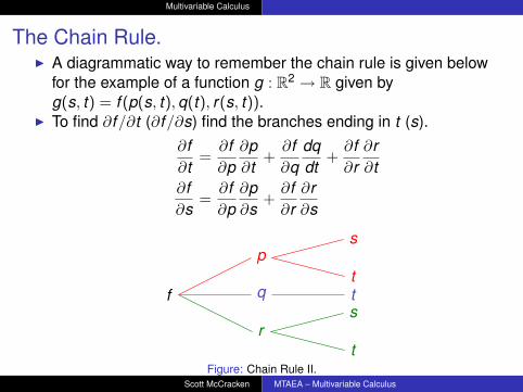
The Chain Rule.I A diagrammatic way to remember the chain rule is given below

for the example of a function g : R2 → R given byg(s, t) = f (p(s, t),q(t), r(s, t)).

I To find ∂f/∂t (∂f/∂s) find the branches ending in t (s).∂f∂t

=∂f∂p

∂p∂t

+∂f∂q

dqdt

+∂f∂r∂r∂t

∂f∂s

=∂f∂p

∂p∂s

+∂f∂r∂r∂s

f

rt

sq t

pt

s

Figure: Chain Rule II.Scott McCracken MTAEA – Multivariable Calculus


The Chain Rule.

ExampleSuppose u = x2 + 2y , where x = r sin(t) and y = sin2(t).

I Note that u = g(r , t) = f (x(r , t), y(r , t)), where f (x , y) = x2 + 2y .

∂u∂r

=∂u∂x

∂x∂r

+∂u∂y

∂y∂r

(=∂g∂r

=∂f∂x

∂x∂r

+∂f∂y

∂y∂r

)= (2x) sin(t) + 2(0) = 2r sin2(t)

∂u∂t

=∂u∂x

∂x∂t

+∂u∂y

∂y∂t

(=∂g∂t

=∂f∂x

∂x∂t

+∂f∂y

∂y∂t

)= (2x)r cos(t) + 2(2 sin(t) cos(t))

= 2(r2 + 2) sin(t) cos(t)



Explicit Functions from Rn to Rm.I Until now we have only looked at derivatives of functions with

one endogenous variable.I Often in economics we are interested in functions with several

endogenous variables.I For example, a firm producing m products using n inputs has a

production funtion for each output:

q1 = f1(x1, . . . , xn)

q2 = f2(x1, . . . , xn)

...qm = fm(x1, . . . , xn).

I We can view the above collection of m functions in n variables asa single function f from Rn to Rm:

f (x) = (f1(x1, . . . , xn), f2(x1, . . . , xn), . . . , fm(x1, . . . , xn)).



Explicit Functions from Rn to Rm.

I Conversely, if we start with a single funtion f : Rn → Rn as above,we see that each component of f is a function from Rn to R.

I Thus it is simple to apply our results for functions from Rn to R,such as the chain rule, to the more general case of functionsfrom Rn to Rm.

I We just apply what we have learnt to each component functionfi : Rn → R and then put it all together in a matrix.

I If, for example, we want to approximate a function f : Rn → Rm

(with component functions f1, . . . , fn) using differentials, we applyour results to each component fi (see p 324 S&B).

I We again obtain a matrix of partial derivatives which representsa linear map giving the linear approximation of f about a point a.



Explicit Functions from Rn to Rm.Definition.Let f : Rn → Rm be a function. The (Jacobian) derivative of f at a,denoted by Df (a) or Dfa, is given by

Df (a) =

∂f1∂x1

(a) ∂f1∂x2

(a) · · · ∂f1∂xn

(a)∂f2∂x1

(a) ∂f2∂x2

(a) · · · ∂f2∂xn

(a)...

.... . .

...∂fm∂x1

(a) ∂fm∂x2

(a) · · · ∂fm∂xn

(a)

. N

I This is sometimes called the Jacobian (matrix). An alternativenotation is

∂(f1, . . . , fm)

∂(x1, . . . , xn).

I When m = n = 1, we simply have the derivative of a functionf : R→ R and denote it as usual by f ′(a).



Explicit Functions from Rn to Rm.ExampleSuppose, there are two commodities with constant elasticity demandfunctions

q1(p1,p2,m) = 2p3

2m2

p1and q2(p1,p2,m) = 3

p21mp2

2

in the vicinity of current prices and income (p∗1,p∗2,m) = (2,4,1). We

want to find out the approximate change in demand for the two goodsas a result of a simultaneous change in prices and income.

I We totally differentiate each component function qi .

dq1 =∂q1

∂p1dp1 +

∂q1

∂p2dp2 +

∂q1

∂mdm

= (−2p−21 p3

2m2)dp1 + (6p−11 p2

2m2)dp2 + (4p−11 p3

2m)dm= −32dp1 + 48dp2 + 32dm at (2,4,1),




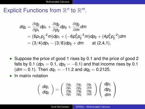
dq2 =∂q2

∂p1dp1 +

∂q2

∂p2dp2 +

∂q2

∂mdm

= (6p1p−22 m)dp1 + (−6p2

1p−32 m)dp2 + (4p2

1p−22 )dm

= (3/4)dp1 − (3/8)dp2 + dm at (2,4,1),

I Suppose the price of good 1 rises by 0.1 and the price of good 2falls by 0.1 (dp1 = 0.1, dp2 = −0.1) and that income rises by 0.1(dm = 0.1). Then dq1 = −11.2 and dq2 = 0.2125.

I In matrix notation(dq1dq2

)=

(∂q1∂p1

∂q1∂p2

∂q1∂m

∂q2∂p1

∂q2∂p2

∂q2∂m

) dp1dp2dm



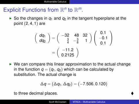
Explicit Functions from Rn to Rm.I So the changes in q1 and q2 in the tangent hyperplane at the

point (2,4,1) are

(dq1dq2

)=

(−32 48 32

34 −3

8 1

) 0.1−0.10.1

=

(−11.20.2125

)I We can compare this linear approximation to the actual change

in the function q = (q1,q2) which can be calculated bysubstitution. The actual change is

∆q = (∆q1,∆q2) = (−7.506,0.120)

to three decimal places. �




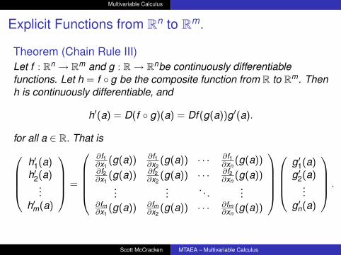
Theorem (Chain Rule III)Let f : Rn → Rm and g : R→ Rnbe continuously differentiablefunctions. Let h = f ◦ g be the composite function from R to Rm. Thenh is continuously differentiable, and

h′(a) = D(f ◦ g)(a) = Df (g(a))g′(a).

for all a ∈ R. That ish′1(a)h′2(a)

...h′m(a)

=

∂f1∂x1

(g(a)) ∂f1∂x2

(g(a)) · · · ∂f1∂xn

(g(a))∂f2∂x1

(g(a)) ∂f2∂x2

(g(a)) · · · ∂f2∂xn

(g(a))...

.... . .

...∂fm∂x1

(g(a)) ∂fm∂x2

(g(a)) · · · ∂fm∂xn

(g(a))

g′1(a)g′2(a)

...g′n(a)

.



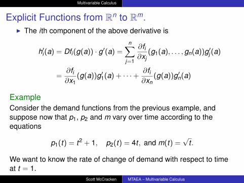
Explicit Functions from Rn to Rm.I The i th component of the above derivative is

h′i (a) = Dfi(g(a)) · g′(a) =n∑

j=1

∂fi∂xj

(g1(a), . . . ,gn(a))g′j (a)

=∂fi∂x1

(g(a))g′1(a) + · · ·+ ∂fi∂xn

(g(a))g′n(a)

ExampleConsider the demand functions from the previous example, andsuppose now that p1, p2 and m vary over time according to theequations

p1(t) = t2 + 1, p2(t) = 4t , and m(t) =√

t .

We want to know the rate of change of demand with respect to timeat t = 1.




I First note that (p1(1),p2(1),m(1)) = (2,4,1). Therefore(dq1dt (1)

dq2dt (1)

)=

(∂q1∂p1

(p(1)) ∂q1∂p2

(p(1)) ∂q1∂m (p(1))

∂q2∂p1

(p(1)) ∂q2∂p2

(p(1)) ∂q2∂m (p(1))

) p′1(1)p′2(1)m′(1)

=

(−32 48 32

34 −3

8 1

) 2412

=

(144

12

)gives the rate of change of demand over time at t = 1. �




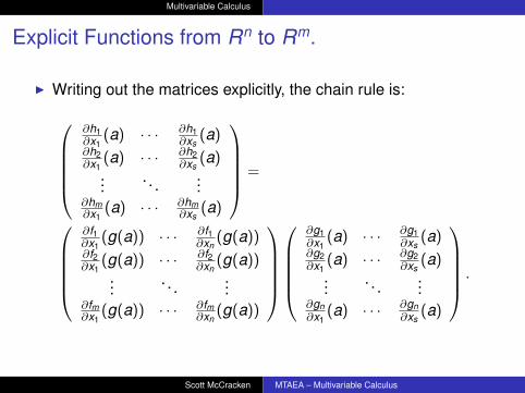
Theorem (Chain Rule IV)Let f : Rn → Rm and g : Rs → Rn be continuously differentiablefunctions. Let h = f ◦ g be the composite function from Rs to Rm.Then h is continuosly differentiable, and

Dh(a) = D(f ◦ g)(a) = Df (g(a))Dg(a).

for all a ∈ Rs.

I Here Df (g(a)) is an m× n Jacobian matrix and Dg(a) is an n× sJacobian matrix.

I The product of these matrices is an m × s Jacobian matrix.I Note that this chain rule is the most general and nests all the

other three.




I Writing out the matrices explicitly, the chain rule is:

∂h1∂x1

(a) · · · ∂h1∂xs

(a)∂h2∂x1

(a) · · · ∂h2∂xs

(a)...

. . ....

∂hm∂x1

(a) · · · ∂hm∂xs

(a)

=

∂f1∂x1

(g(a)) · · · ∂f1∂xn

(g(a))∂f2∂x1

(g(a)) · · · ∂f2∂xn

(g(a))...

. . ....

∂fm∂x1

(g(a)) · · · ∂fm∂xn

(g(a))

∂g1∂x1

(a) · · · ∂g1∂xs

(a)∂g2∂x1

(a) · · · ∂g2∂xs

(a)...

. . ....

∂gn∂x1

(a) · · · ∂gn∂xs

(a)

.



Higher Order Derivatives.I The partial derivative ∂f/∂xi of a function given by f (x1, . . . , xn)is

itself a function of n variables. We can continue taking partialderivatives of these partial derivatives.

I Sometimes it is not possible to partially differentiate a functionwith respect to some variable. So we need some terminologydescribing how “smooth” functions are.

Definition.Let U be an open subset of Rn and let f : Rn → R be a function.

I We say f is k -times differentiable at a ∈ U if all its partialderivatives of order less than k exist. If this is true for all a ∈ U,we say f is k -times differentiable on U.

I We say f is k -times continuously differentiable or Ck at a if all itspartial derivatives exist and are continuous at a. If this is true forall a ∈ U, we say f is k -times continuously differentiable or Ck onU. N



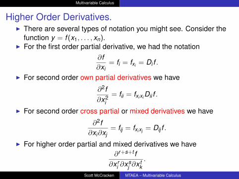
Higher Order Derivatives.I There are several types of notation you might see. Consider the

function y = f (x1, . . . , xn).I For the first order partial derivative, we had the notation

∂f∂xi

= fi = fxi = Di f .

I For second order own partial derivatives we have

∂2f∂x2

i= fii = fxi xi Dii f .

I For second order cross partial or mixed derivatives we have

∂2f∂xi∂xj

= fij = fxi xj = Dij f .

I For higher order partial and mixed derivatives we have∂r+s+t f

∂x ri ∂xs

j ∂x tk.



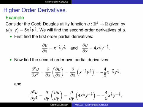
Higher Order Derivatives.ExampleConsider the Cobb-Douglas utility function u : R2 → R given byu(x , y) = 5x

15 y

45 . We will find the second-order derivatives of u.

I First find the first order partial derivatives:

∂u∂x

= x−45 y

45 and

∂u∂y

= 4x15 y−

15 .

I Now find the second order own partial derivatives:

∂2u∂x2 =

∂

∂x

(∂u∂x

)=

∂

∂x

(x−

45 y

45

)= −4

5x−

95 y

45 ,

and

∂2u∂y2 =

∂

∂y

(∂u∂y

)=

∂

∂y

(4x

15 y−

15

)= −4

5x

15 y−

65 ,



Higher Order Derivatives.

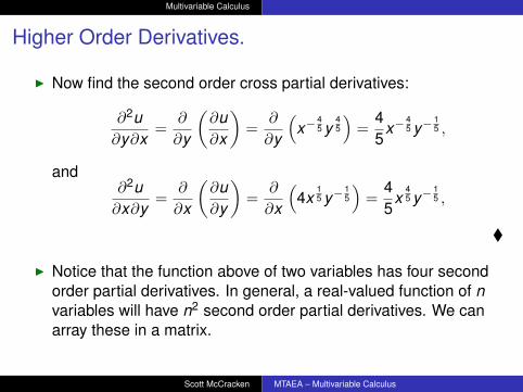
I Now find the second order cross partial derivatives:

∂2u∂y∂x

=∂

∂y

(∂u∂x

)=

∂

∂y

(x−

45 y

45

)=

45

x−45 y−

15 ,

and∂2u∂x∂y

=∂

∂x

(∂u∂y

)=

∂

∂x

(4x

15 y−

15

)=

45

x45 y−

15 ,

�

I Notice that the function above of two variables has four secondorder partial derivatives. In general, a real-valued function of nvariables will have n2 second order partial derivatives. We canarray these in a matrix.



Higher Order Derivatives.

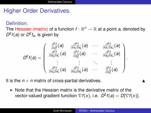
Definition.The Hessian (matrix) of a function f : Rn → R at a point a, denoted byD2f (a) or D2fa, is given by

D2f (a) =

∂2f∂x2

1(a) ∂2f

∂x1∂x2(a) · · · ∂2f

∂x1∂xn(a)

∂2f∂x2∂x1

(a) ∂2f∂x2

2(a) · · · ∂2f

∂x2∂xn(a)

......

. . ....

∂2f∂xn∂x1

(a) ∂2f∂xn∂x2

(a) · · · ∂2f∂x2

n(a)

.

It is the n × n matrix of cross-partial derivatives. N

I Note that the Hessian matrix is the derivative matrix of thevector-valued gradient function ∇f (x), i.e. D2f (a) = D[∇f (x)].



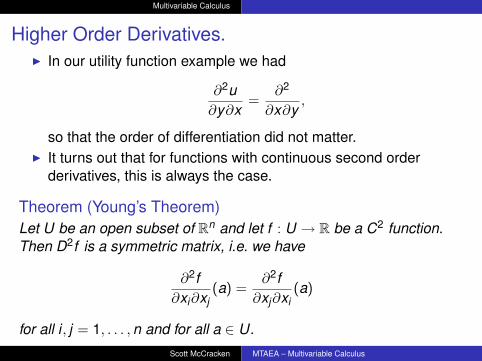
Higher Order Derivatives.I In our utility function example we had

∂2u∂y∂x

=∂2

∂x∂y,

so that the order of differentiation did not matter.I It turns out that for functions with continuous second order

derivatives, this is always the case.

Theorem (Young’s Theorem)Let U be an open subset of Rn and let f : U → R be a C2 function.Then D2f is a symmetric matrix, i.e. we have

∂2f∂xi∂xj

(a) =∂2f∂xj∂xi

(a)

for all i , j = 1, . . . ,n and for all a ∈ U.Scott McCracken MTAEA – Multivariable Calculus


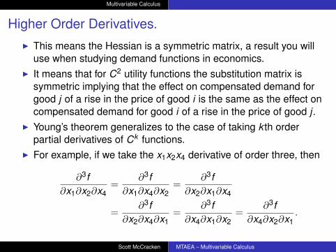
Higher Order Derivatives.I This means the Hessian is a symmetric matrix, a result you will

use when studying demand functions in economics.I It means that for C2 utility functions the substitution matrix is

symmetric implying that the effect on compensated demand forgood j of a rise in the price of good i is the same as the effect oncompensated demand for good i of a rise in the price of good j .

I Young’s theorem generalizes to the case of taking k th orderpartial derivatives of Ck functions.

I For example, if we take the x1x2x4 derivative of order three, then

∂3f∂x1∂x2∂x4

=∂3f

∂x1∂x4∂x2=

∂3f∂x2∂x1∂x4

=∂3f

∂x2∂x4∂x1=

∂3f∂x4∂x1∂x2

=∂3f

∂x4∂x2∂x1.


MTAEA Multivariable Calculus - Scott McCracken · 2019-11-18 · Multivariable Calculus Geometric...

Documents

Transcript of MTAEA Multivariable Calculus - Scott McCracken · 2019-11-18 · Multivariable Calculus Geometric...