MSEG 803Equilibria in Material Systems

7: Statistical Interpretation of S

Prof. Juejun (JJ) Hu

hujuejun@udel.edu

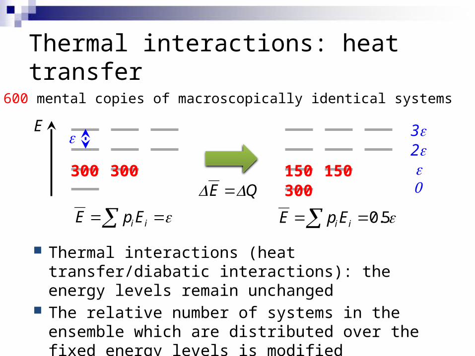
Thermal interactions: heat transfer

Thermal interactions (heat transfer/diabatic interactions): the energy levels remain unchanged

The relative number of systems in the ensemble which are distributed over the fixed energy levels is modified

300 300

600 mental copies of macroscopically identical systems

Ee

150 150300

i iE p E 0.5i iE p E

3e2ee0E Q

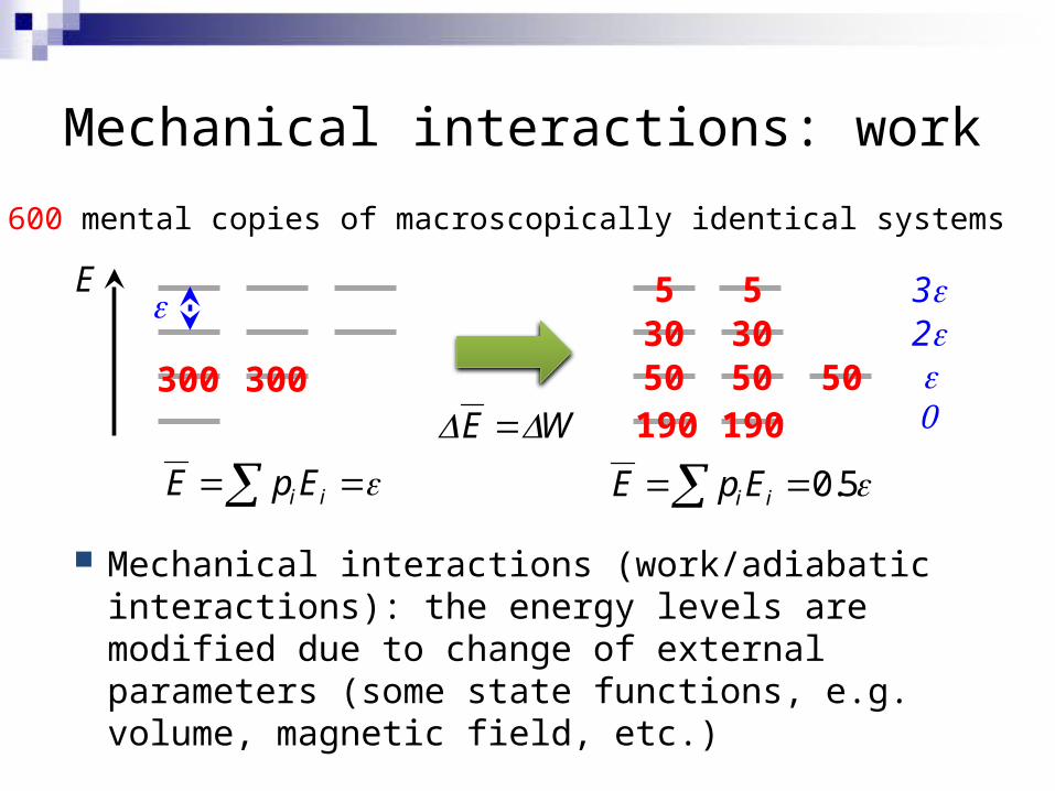
Mechanical interactions: work

Mechanical interactions (work/adiabatic interactions): the energy levels are modified due to change of external parameters (some state functions, e.g. volume, magnetic field, etc.)

300 300

Ee

50 50190

i iE p E 0.5i iE p E

3e2ee0190

5030 30

55

E W

600 mental copies of macroscopically identical systems

General interactions

Ensemble average of system energy: First law of TD:

Quasi-static work:

Mean generalized force:

dU dE Q W i iU E p E

i i i i i idE d p E p dE E dp Heat: population

distribution changeWork: energy level change

i ii i i i

dE dEW p dE p dx dx p y dx

dx dx

ii

dE dEy p

dx dx

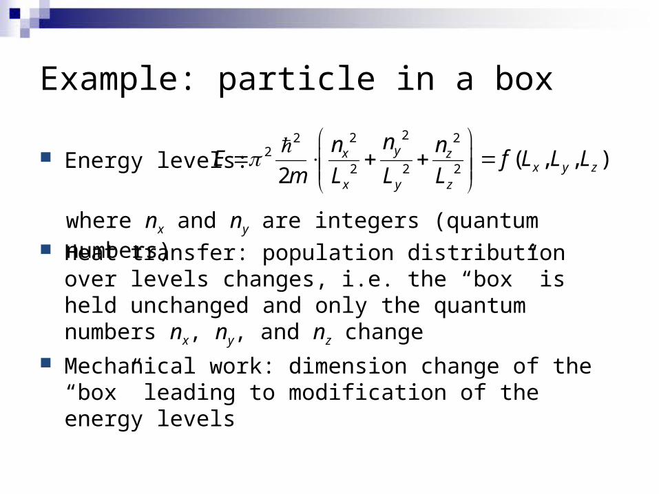
Example: particle in a box

Energy levels:

Heat transfer: population distribution over levels changes, i.e. the “box” is held unchanged and only the quantum numbers nx, ny, and nz change

Mechanical work: dimension change of the “box” leading to modification of the energy levels

22 222

2 2 2( , , )

2yx z

x y zx y z

nn nE f L L L

m L L L

where nx and ny are integers (quantum numbers)

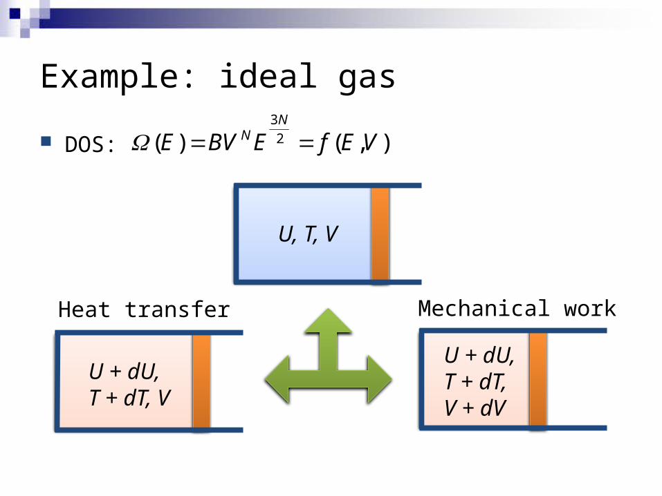
Example: ideal gas

DOS:3

2( ) ( , )N

NE BV E f E V

U, T, V

U + dU,T + dT, V

U + dU,T + dT,V + dV

Heat transfer Mechanical work

Equilibrium condition in isolated systems

DOS of a composite isolated system consisting of sub-systems:

xi: external parameters

yi: internal constraints (usually extensive variables of sub-systems)

Example: ideal gas in a cylinder with a partition Internal constraint y: mole number in the sub-systems Accessible states only include those satisfy the constraint, i.e. all gas

molecules have to reside on the left side of the partition

1 2 1 2( , ,..., , , ,..., )n nf x x x y y y

N, Vi

Equilibrium condition in isolated systems

Removal of constraint(s) leads to increased (or possibly unchanged) number of accessible states and re-distribution of some extensive parameter(s)

Probability of the system remaining in the constrained states:

Example: ideal gas in a cylinder with a partition Accessible states now include all states where gas molecules are

free to distribute in the entire cylinder

N, Vi

Remove constraint

f i

~ 0i i fP

N, Vf > Vi

Equilibrium condition in isolated systems

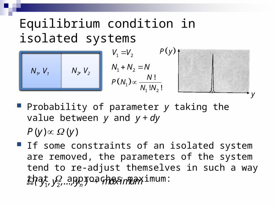
Probability of parameter y taking the value between y and y + dy

If some constraints of an isolated system are removed, the parameters of the system tend to re-adjust themselves in such a way that W approaches maximum:

( ) ( )P y y

N1, V1 N2, V2

1 2V V

1 2 n( y , y ,..., y ) max imum

1 2N N N

11 2

!

! !

NP N

N N

P y

y

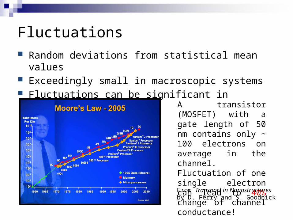
Fluctuations Random deviations from statistical mean values Exceedingly small in macroscopic systems Fluctuations can be significant in nanoscale systems

A transistor (MOSFET) with a gate length of 50 nm contains only ~ 100 electrons on average in the channel. Fluctuation of one single electron can lead to 40% change of channel conductance!From Transport in Nanostructures by D. Ferry and S. Goodnick

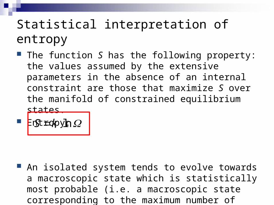
Statistical interpretation of entropy

The function S has the following property: the values assumed by the extensive parameters in the absence of an internal constraint are those that maximize S over the manifold of constrained equilibrium states.

Entropy:

An isolated system tends to evolve towards a macroscopic state which is statistically most probable (i.e. a macroscopic state corresponding to the maximum number of microscopic accessible states)

lnS k

Thermal equilibrium

Two sub-systems separated by a

rigid, diathermal wall

Apply the maximum principle of W

A B

Isolated composite system

dQ

1 2totU U U cons tant

1 1 2 2tot U U

0totd 1 2ln ln ln 0totd d d

1 2 1 21 2 1

1 2 1 2

ln ln ln lnln 0totd dU dU dU

U U U U

1 2

1 2

ln ln

U U

ln 1

( )UU kT

1 2T T

1tot U

1U

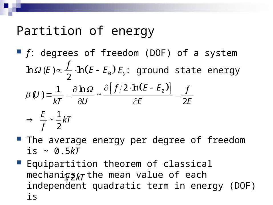
Partition of energy

f: degrees of freedom (DOF) of a system

The average energy per degree of freedom is ~ 0.5kT Equipartition theorem of classical mechanics: the mean

value of each independent quadratic term in energy (DOF) is

02 ln1 ln( ) ~

2

f E E fU

kT U E E

0ln ( ) ln2

fE E E E0: ground state energy

1~2

EkT

f

1 2kT

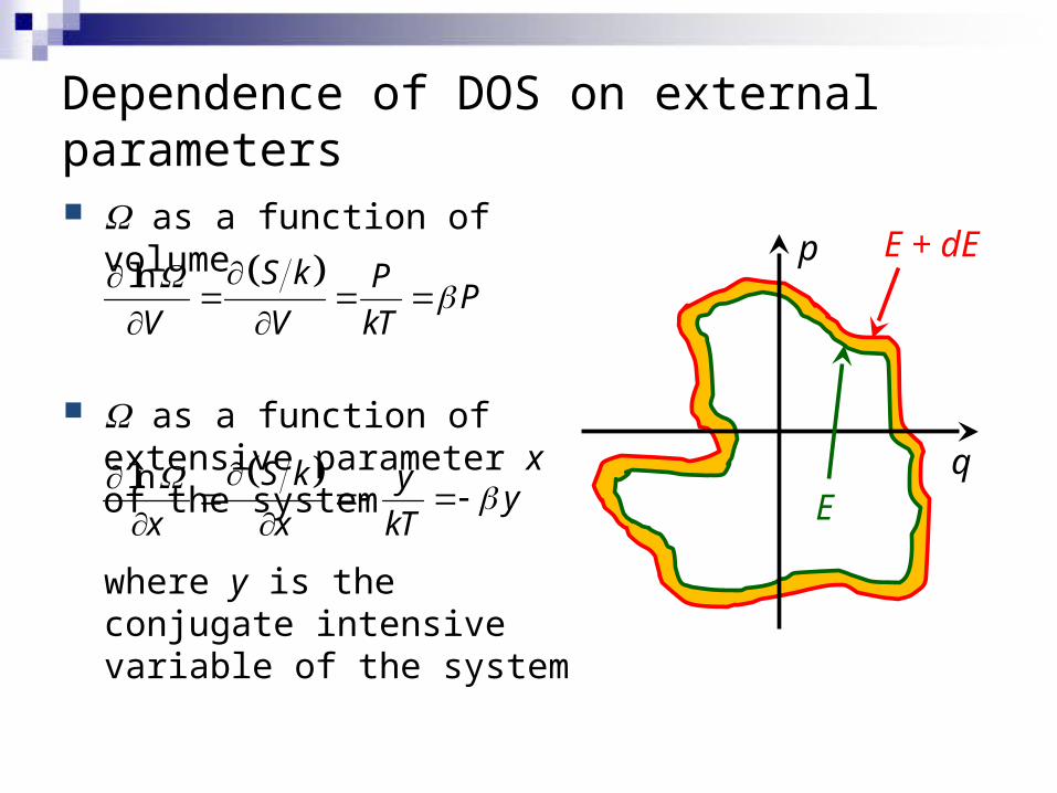
Dependence of DOS on external parameters

W as a function of volume

W as a function of extensive parameter x of the system

ln S k PP

V V kT

q

p

E

E + dE

ln S k yy

x x kT

where y is the conjugate intensive variable of the system

The 3rd law of thermodynamics

At absolute zero (T = 0 K), the system is “frozen” into its quantum mechanical ground state

where W is the degeneracy of the ground state

( 0 ) ln ~ 0S T K k

The Third Law of Thermodynamicsby Katharine A. Cartwright (2010)watercolor on paper26" x 20”

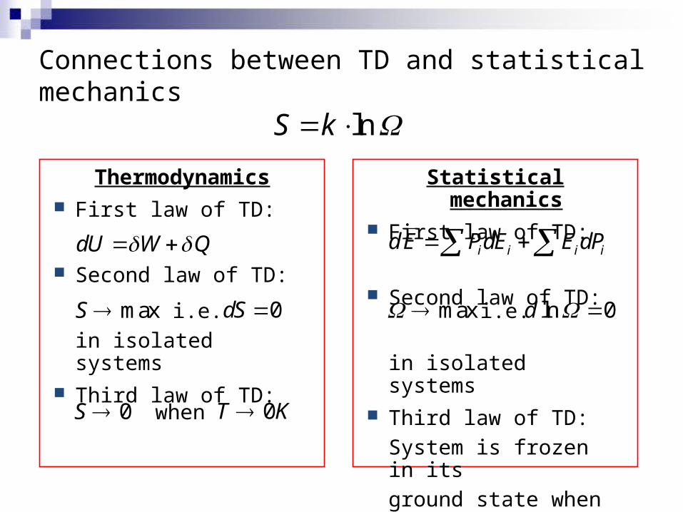
Connections between TD and statistical mechanics

Thermodynamics First law of TD:

Second law of TD:

in isolated systems Third law of TD:

dU W Q

0dS maxS i.e.

0T K0S when

Statistical mechanics First law of TD:

Second law of TD:

in isolated systems Third law of TD:

System is frozen in its

ground state when T = 0

i i i idE PdE E dP

ln 0d max i.e.

lnS k