MS&E 211 Minimum Cost Flow LP Ashish Goel. Minimum Cost Flow (MCF) Need to ship some good from...
73
MS&E 211 Minimum Cost Flow LP Ashish Goel
-
Upload
magdalene-joseph -
Category
Documents
-
view
221 -
download
1
Transcript of MS&E 211 Minimum Cost Flow LP Ashish Goel. Minimum Cost Flow (MCF) Need to ship some good from...

MS&E 211Minimum Cost Flow LP
Ashish Goel

Minimum Cost Flow (MCF)
• Need to ship some good from “supply” nodes to “demand” nodes over a network– Example: the good could be crude oil; the network could
be a network of pipelines; the supply nodes could be oil fields; the demand nodes could be refineries
• Assumption: The good is divisible, so we can ship fractional amounts of a good over an edge
• Fundamental problem: generalizes shortest paths; maximum compatibility matching; max-flow; and several problems we have seen already

Modeling the Network
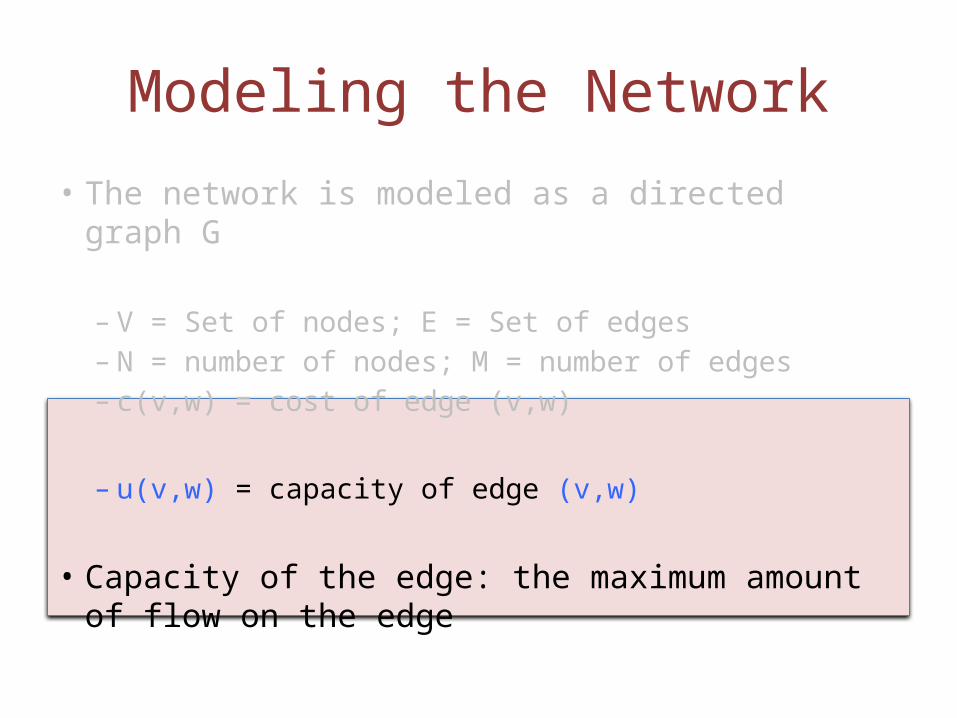
• The network is modeled as a directed graph G
– V = Set of nodes; E = Set of edges– N = number of nodes; M = number of edges– c(v,w) = cost of edge (v,w)
– u(v,w) = capacity of edge (v,w)
• Capacity of the edge: the maximum amount of flow on the edge

Modeling the Network
• The network is modeled as a directed graph G
– V = Set of nodes; E = Set of edges– N = number of nodes; M = number of edges– c(v,w) = cost of edge (v,w)
– u(v,w) = capacity of edge (v,w)
• Capacity of the edge: the maximum amount of flow on the edge
Modeling the Network
• The network is modeled as a directed graph G
– V = Set of nodes; E = Set of edges– N = number of nodes; M = number of edges– c(v,w) = cost of edge (v,w)
– u(v,w) = capacity of edge (v,w)
• Capacity of the edge: the maximum amount of flow on the edge

Modeling Demands
• Demand of a node: The amount of the good that a node wants to consume
• Supply of a node: The amount of the good that a node wants to produce
• Modeled as a single number, d(v), for node v– d(v) is positive for “demand nodes”– d(v) is negative for “supply nodes”– d(v) = 0 otherwise
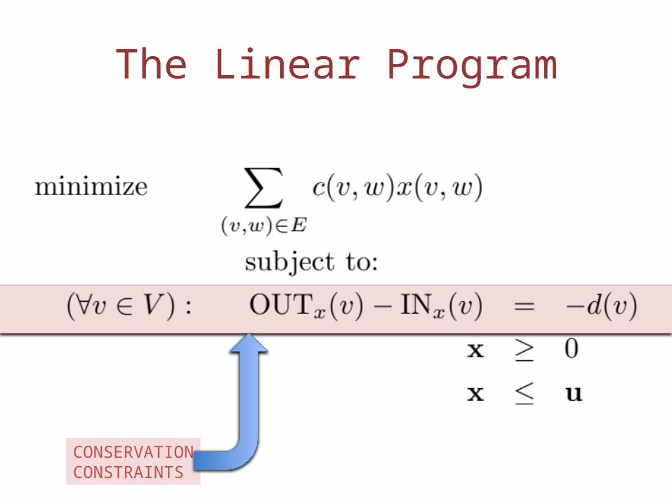
The Linear Program
CONSERVATIONCONSTRAINTS

The Linear Program
CAPACITYCONSTRAINTS
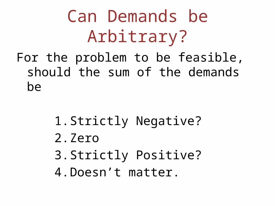
Can Demands be Arbitrary?
For the problem to be feasible, should the sum of the demands be
1. Strictly Negative?2. Zero3. Strictly Positive?4. Doesn’t matter.
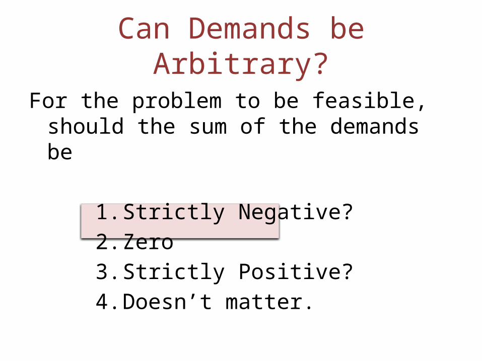
Can Demands be Arbitrary?
For the problem to be feasible, should the sum of the demands be
1. Strictly Negative?2. Zero3. Strictly Positive?4. Doesn’t matter.

The Linear Program
SUMS TO ZERO, WHEN SUMMEDOVER ALL NODES
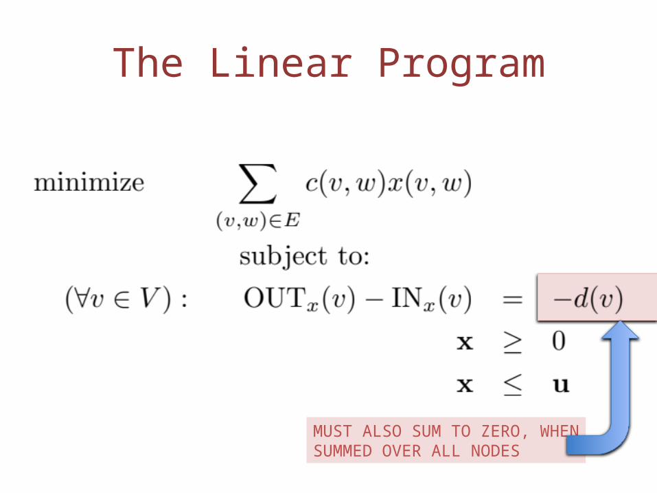
The Linear Program
MUST ALSO SUM TO ZERO, WHENSUMMED OVER ALL NODES

Reduction to MCF
• Very powerful tool• Suppose we are reducing a problem P to MCF• Must specify how to obtain– The graph G (nodes, edges)– Edge capacities u and costs c– Node demands d
from the parameters of the given problem P• Must specify how the solution x to MCF gives a
solution to P

A Simple Reduction
• Reducing Shortest Paths to MCF– Use the same graph G– Set d(s) = -1, d(t) = 1, d(v) = 0 for all other nodes– Set u(v,w) = 1 for all edges (v,w)
(Or, set u(v,w) = ∞ for all edges (v,w))– The solution x(v,w) to the MCF is also a solution to
the shortest path problem• Hence, MCF is more general than shortest
paths

A Simple Example
Every edge has a cost and a capacity, written as (c, u)
(6,1)
(2,1)
(4,1)
st
p
qr
(1,1)
(2,1)
(3,1)
(4,1)

A Simple Example
Every node has a demand
(6,1)
(2,1)
(4,1)
st
p
qr
(1,1)
(2,1)
(3,1)
(4,1)
d = -1d = 1
d = 0
d = 0
d = 0

A Simple Example
Every node has a demand
(6, ∞)
(2, ∞)
(4, ∞)
st
p
qr
(1, ∞)
(2, ∞)
(3, ∞)
(4,∞)
d = -1d = 1
d = 0
d = 0
d = 0

Infinite Capacities?
• Can handle infinite capacity edges by just removing the capacity constraint for those edges
• For shortest paths– Setting capacity = ∞ guarantees that there will
never be an optimum solution if there is a negative cost cycle
– Setting capacity = 1 guarantees that there will be an optimum solution if there is a feasible solution
Next Steps
• Theory: Examine Basic Feasible Solutions
• Reductions: See two more examples
• Hands On: Solve the Shortest Path Problem again– Illustrate capacity constraints– A nice trick for generating the constraint matrix A

Minimum Cost Flow – Basic Feasible Solutions
Ashish Goel

Main Theorem
For an instance of a Minimum Cost Flow Problem, if
(a) Every demand is integraland
(b) Every capacity is integralthen
Every Basic Feasible Solution is Integral
• Very useful, since in many applications (eg. Shortest paths), fractional solutions do not make sense

Proof Sketch
1. Start with any feasible fractional solution
2. Find a cycle of edges (ignoring directions) such that every edge on the cycle has fractional flow
3. Show that along this cycle, flow can be increased a little clockwise, as well as counterclockwise
The original fractional solution was an average of two other feasible solutions, and hence not a BFS

A Simple Example
Labels on edges are (costs, capacities)
(6,1)
(2,1)
(4,1)
st
p
qr
(1,1)
(2,1)
(3,1)
(4,1)
d = -1d = 1
d = 0
d = 0
d = 0

Step 1: Start With a Fractional Solution
Labels on edges are flows
0.6
0
0
st
p
qr
0.4
0.4
0.4
0.6
d = -1d = 1
d = 0
d = 0
d = 0
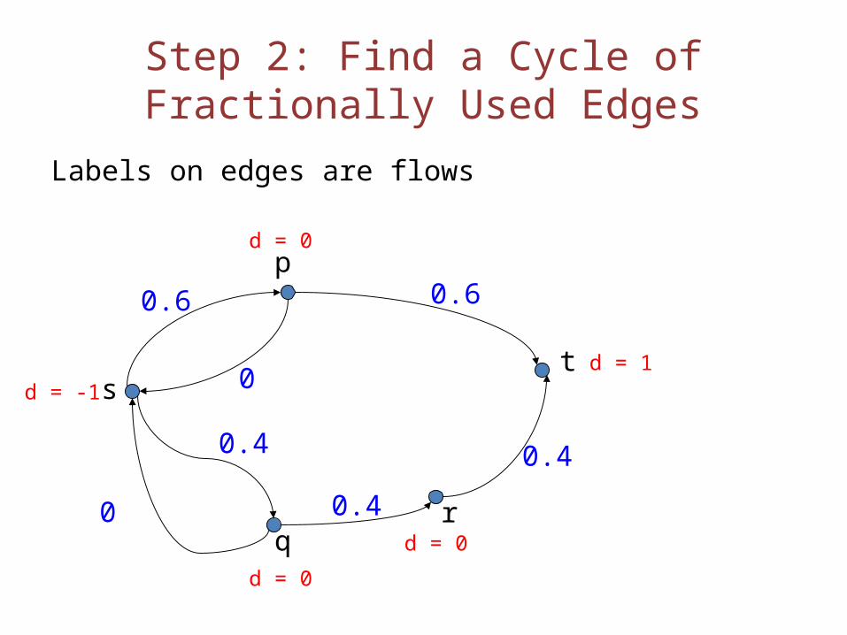
Step 2: Find a Cycle of Fractionally Used Edges
Labels on edges are flows
0.6
0
0
st
p
qr
0.4
0.4
0.4
0.6
d = -1d = 1
d = 0
d = 0
d = 0

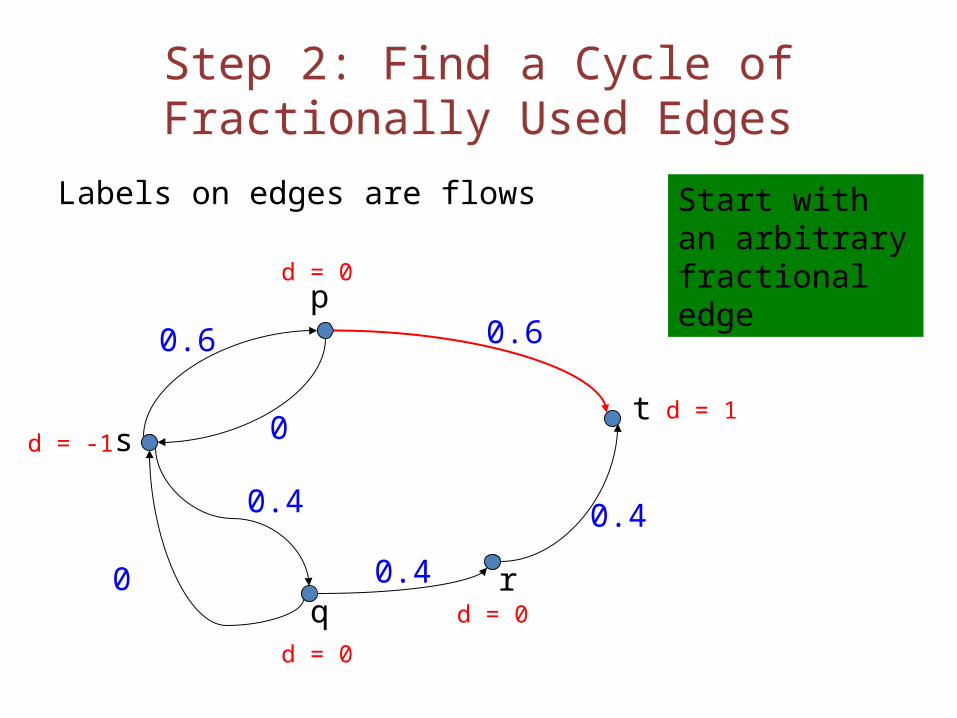
Step 2: Find a Cycle of Fractionally Used Edges
Labels on edges are flows
0.6
0
0
st
p
qr
0.4
0.4
0.4
0.6
d = -1d = 1
d = 0
d = 0
d = 0
Start with an arbitrary fractional edge
Step 2: Find a Cycle of Fractionally Used Edges
Labels on edges are flows
0.6
0
0
st
p
qr
0.4
0.4
0.4
0.6
d = -1d = 1
d = 0
d = 0
d = 0
Start with an arbitrary fractional edge

Step 2: Find a Cycle of Fractionally Used Edges
Labels on edges are flows
0.6
0
0
st
p
qr
0.4
0.4
0.4
0.6
d = -1d = 1
d = 0
d = 0
d = 0
Since t has integer demand, there must be another edge incident on t with fractional flow

Step 2: Find a Cycle of Fractionally Used Edges
Labels on edges are flows
0.6
0
0
st
p
qr
0.4
0.4
0.4
0.6
d = -1d = 1
d = 0
d = 0
d = 0
Since t has integer demand, there must be another edge incident on t with fractional flow

Step 2: Find a Cycle of Fractionally Used Edges
Labels on edges are flows
0.6
0
0
st
p
qr
0.4
0.4
0.4
0.6
d = -1d = 1
d = 0
d = 0
d = 0
Use the same argument at r

Step 2: Find a Cycle of Fractionally Used Edges
Labels on edges are flows
0.6
0
0
st
p
qr
0.4
0.4
0.4
0.6
d = -1d = 1
d = 0
d = 0
d = 0
Use the same argument at r

Step 2: Find a Cycle of Fractionally Used Edges
Labels on edges are flows
0.6
0
0
st
p
qr
0.4
0.4
0.4
0.6
d = -1d = 1
d = 0
d = 0
d = 0
Use the same argument at q

Step 2: Find a Cycle of Fractionally Used Edges
Labels on edges are flows
0.6
0
0
st
p
qr
0.4
0.4
0.4
0.6
d = -1d = 1
d = 0
d = 0
d = 0
Use the same argument at q

Step 2: Find a Cycle of Fractionally Used Edges
Labels on edges are flows
0.6
0
0
st
p
qr
0.4
0.4
0.4
0.6
d = -1d = 1
d = 0
d = 0
d = 0
Use the same argument at s

Step 2: Find a Cycle of Fractionally Used Edges
Labels on edges are flows
0.6
0
0
st
p
qr
0.4
0.4
0.4
0.6
d = -1d = 1
d = 0
d = 0
d = 0
Use the same argument at s

Step 2: Find a Cycle of Fractionally Used Edges
Labels on edges are flows
0.6
0
0
st
p
qr
0.4
0.4
0.4
0.6
d = -1d = 1
d = 0
d = 0
d = 0
We have our cycle

Step 2: Find a Cycle of Fractionally Used Edges
Labels on edges are flows
0.6
0
0
st
p
qr
0.4
0.4
0.4
0.6
d = -1d = 1
d = 0
d = 0
d = 0
We have our cycle
Strongly used the fact that demands are integer

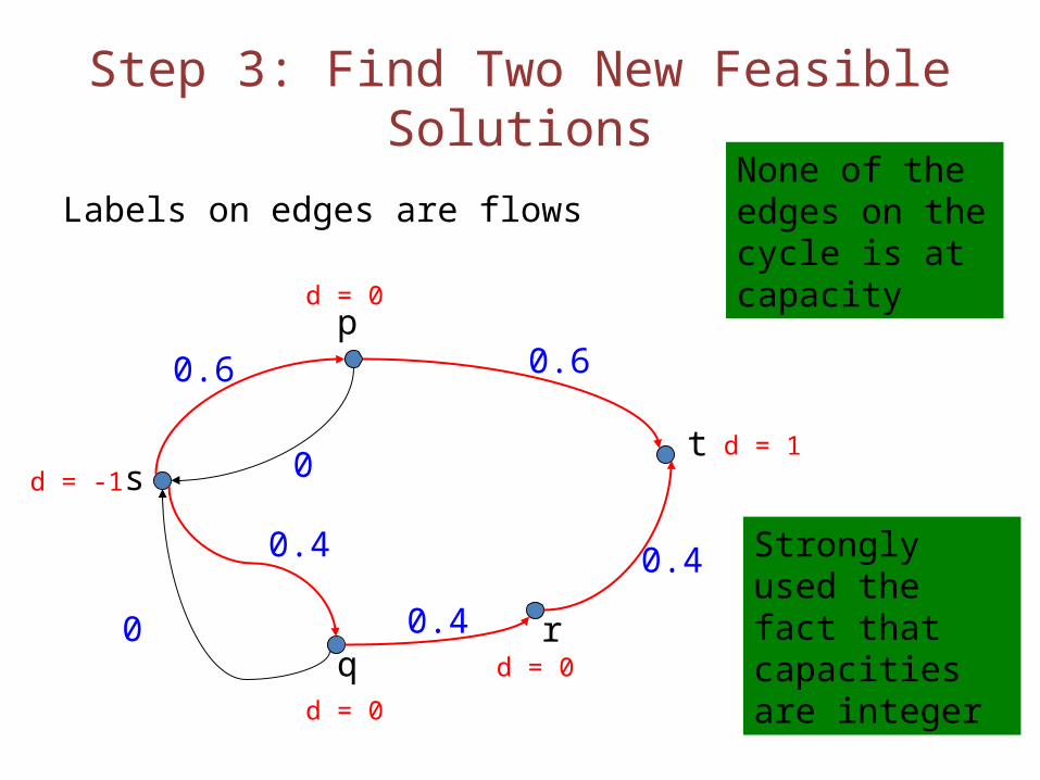
Step 3: Find Two New Feasible Solutions
Labels on edges are flows
0.6
0
0
st
p
qr
0.4
0.4
0.4
0.6
d = -1d = 1
d = 0
d = 0
d = 0
None of the edges on the cycle is at capacity
Step 3: Find Two New Feasible Solutions
Labels on edges are flows
0.6
0
0
st
p
qr
0.4
0.4
0.4
0.6
d = -1d = 1
d = 0
d = 0
d = 0
None of the edges on the cycle is at capacity
Strongly used the fact that capacities are integer

Step 3: Find Two New Feasible Solutions
Labels on edges are flows
0.6
0
0
st
p
qr
0.4
0.4
0.4
0.6
d = -1d = 1
d = 0
d = 0
d = 0
Each edge on the cycle has non-zero flow

Step 3: Find Two New Feasible Solutions
Labels on edges are flows
0.6
0
0
st
p
qr
0.4
0.4
0.4
0.6
d = -1d = 1
d = 0
d = 0
d = 0
Each edge on the cycle has non-zero flow
Hence, can increase or decrease the flow on each edge

Step 3: Find Two New Feasible Solutions
Labels on edges are flows
0.6
0
0
st
p
qr
0.4
0.4
0.4
0.6
d = -1d = 1
d = 0
d = 0
d = 0
Send some flow (say 0.1) “clockwise”
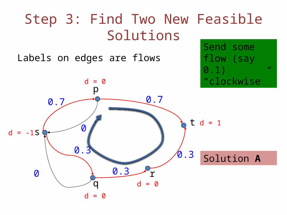
Step 3: Find Two New Feasible Solutions
Labels on edges are flows
0.7
0
0
st
p
qr
0.3
0.3
0.3
0.7
d = -1d = 1
d = 0
d = 0
d = 0
Send some flow (say 0.1) “clockwise”
Solution A

Step 3: Find Two New Feasible Solutions
Labels on edges are flows
0.6
0
0
st
p
qr
0.4
0.4
0.4
0.6
d = -1d = 1
d = 0
d = 0
d = 0
Send some flow (say 0.1) “counter-clockwise”
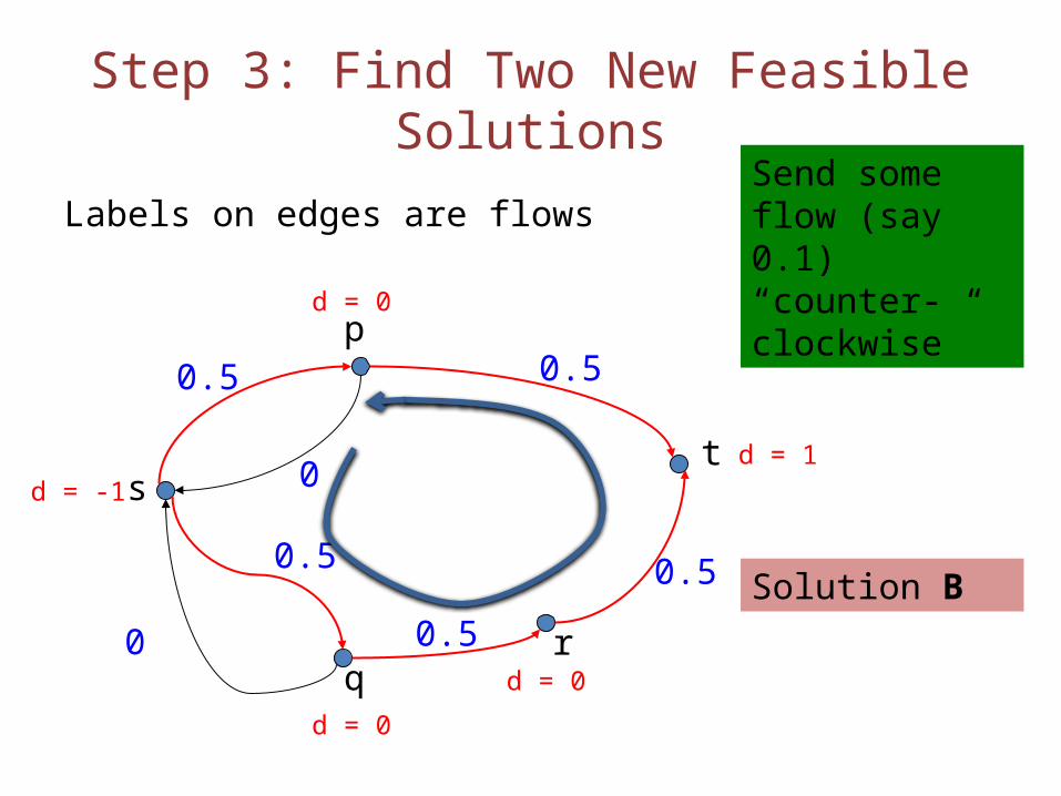
Step 3: Find Two New Feasible Solutions
Labels on edges are flows
0.5
0
0
st
p
qr
0.5
0.5
0.5
0.5
d = -1d = 1
d = 0
d = 0
d = 0
Send some flow (say 0.1) “counter-clockwise”
Solution B

Step 3: Find Two New Feasible Solutions
Labels on edges are flows
0.6
0
0
st
p
qr
0.4
0.4
0.4
0.6
d = -1d = 1
d = 0
d = 0
d = 0
The average of Solutions A and B gives us the fractional solution we started with

Step 3: Find Two New Feasible Solutions
Labels on edges are flows
0.6
0
0
st
p
qr
0.4
0.4
0.4
0.6
d = -1d = 1
d = 0
d = 0
d = 0
The average of Solutions A and B gives us the fractional solution we started with
Hence, we did not start with a BFS

While we used a specific example, the proof is completely generalizable for any MCF with integer capacities and demands
Main Theorem
For an instance of a Minimum Cost Flow Problem, if
(a) Every demand is integraland
(b) Every capacity is integralthen
Every Basic Feasible Solution is Integral
• Very useful, since in many applications (eg. Shortest paths), fractional solutions do not make sense

Minimum Cost Flow – Two Reductions
Ashish Goel

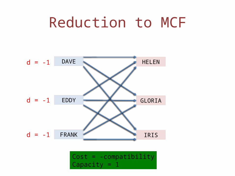
Example: Matching
• Marry every man to exactly one woman, and vice-versa, while maximizing total compatibility
Ci,j : Compatibility of man i with woman j
COMPATIBILTY Helen Gloria Iris
Dave 1 0 0.5
Eddy 0.75 2 1
Frank 0.5 2.5 1.5

Reduction to MCF
DAVE
EDDY
FRANK
HELEN
GLORIA
IRIS

Reduction to MCF
DAVE
EDDY
FRANK
HELEN
GLORIA
IRIS
Cost = -compatibilityCapacity = 1

Reduction to MCF
DAVE
EDDY
FRANK
HELEN
GLORIA
IRIS
Cost = -compatibilityCapacity = 1
WHAT SHOULDTHE DEMAND OFDAVE BE IN THISPROBLEM?
Reduction to MCF
DAVE
EDDY
FRANK
HELEN
GLORIA
IRIS
Cost = -compatibilityCapacity = 1
d = -1
d = -1
d = -1

Reduction to MCF
DAVE
EDDY
FRANK
HELEN
GLORIA
IRIS
Cost = -compatibilityCapacity = 1
d = -1
d = -1
d = -1
WHAT SHOULDTHE DEMAND OFIRIS BE IN THISPROBLEM?
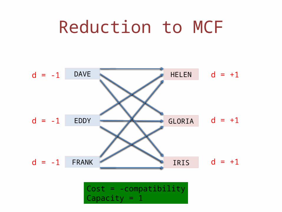
Reduction to MCF
DAVE
EDDY
FRANK
HELEN
GLORIA
IRIS
Cost = -compatibilityCapacity = 1
d = -1
d = -1
d = -1
d = +1
d = +1
d = +1

Reduction to MCF
DAVE
EDDY
FRANK
HELEN
GLORIA
IRIS
Cost = -compatibilityCapacity = 1
d = -1
d = -1
d = -1
d = +1
d = +1
d = +1
x(v,w) The amount ofmarriage betweenman v and woman w
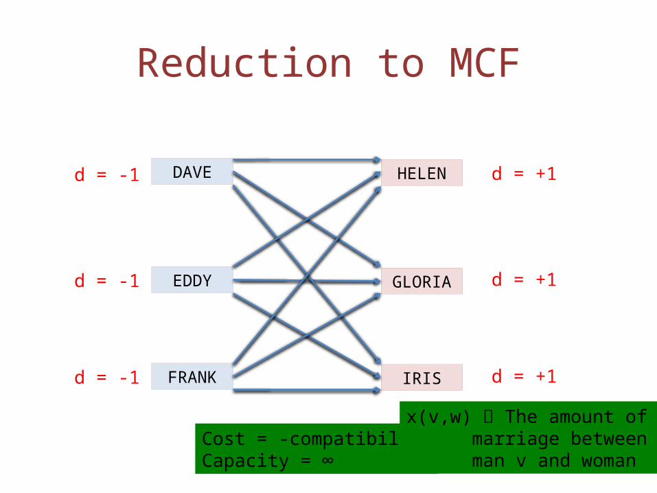
Reduction to MCF
DAVE
EDDY
FRANK
HELEN
GLORIA
IRIS
Cost = -compatibilityCapacity = ∞
d = -1
d = -1
d = -1
d = +1
d = +1
d = +1
x(v,w) The amount ofmarriage betweenman v and woman w

Basic Feasible Solutions for Matchings
• Any BFS for the Maximum Compatibility Matching problem written as a MCF must be an integer– Integer capacities and demands
• Interesting observation: The LP for the Maximum Compatibility Matching that we saw earlier is exactly the same as the LP for the corresponding MCF
(s,t) Max-Flow Problem
• Given a directed graph G with capacities (but no costs) on edges
• Given two special nodes in V: a source s and a terminus t
• Find the maximum amount of flow that can be sent from s to t

ExampleLabels on edges represent capacities, not costs
Eyeballing: Optimum solution is to send 4 units of flow on top path, and 1 unit on bottom path
6
2
4
st
p
qr
1
2
3
4
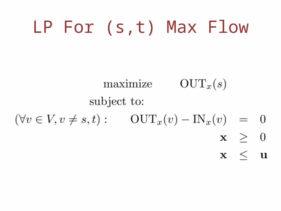
LP For (s,t) Max Flow
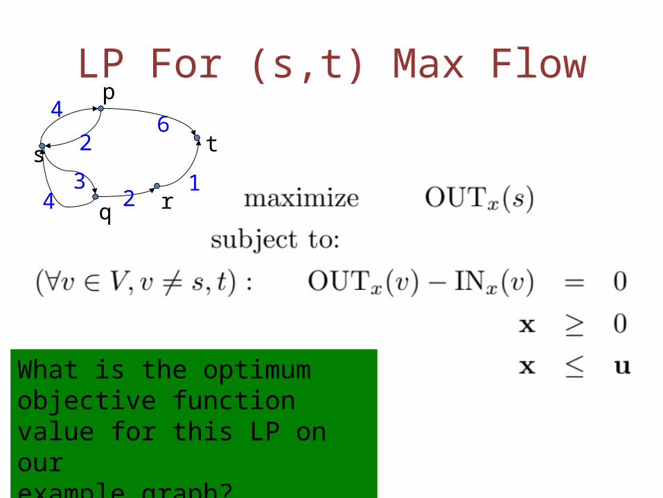
LP For (s,t) Max Flow
What is the optimum objective function value for this LP on ourexample graph?
62
4
s t
q r1
23
4p

LP For (s,t) Max Flow
What is the optimum objective function value for this LP on ourexample graph? Answer: 7 Not correct LP
62
4
s t
q r1
23
4p

LP For (s,t) Max Flow

Reduction to MCF
• Start with an instance of the max-flow problem– Graph G with edge capacities– Missing: edge costs; node demands– Set each edge cost to 0, each node demand to 0
• Add a new edge from t to s of infinite capacity and cost -1, to obtain an instance of MCF
• Intuition: MCF solution will try to minimize cost by pushing as much flow as possible from t to s– Since demands are all zero, this flow must travel back from s to t
using edges in the original graph G

Example Reduction to MCF
Start with max-flow problem: Labels on edges are (capacities)
(6)
(2)
(4)
st
p
qr(2)
(3)
(4)
(1)

Example Reduction to MCF
Make edge costs 0: Labels on edges are (cost, capacity)
(0, 6)
(0,2)
(0,4)
st
p
qr(0,2)
(0,3)
(0, 4)
(0,1)

Example Reduction to MCF
Add demands of 0
(0, 6)
(0,2)
(0,4)
st
p
qr(0,2)
(0,3)
(0, 4)
d = 0d = 0
d = 0
d = 0
d = 0
(0,1)
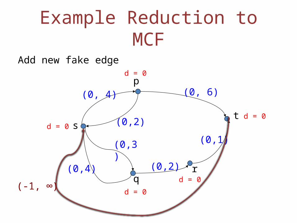
Example Reduction to MCF
Add new fake edge
(0, 6)
(0,2)
(0,4)
st
p
qr
(0,1)
(0,2)
(0,3)
(0, 4)
d = 0d = 0
d = 0
d = 0
d = 0(-1, ∞)

Basic Feasible Solutions
• If each capacity in the (s,t) max-flow problem is integral, then any BFS to the resulting MCF problem LP is integral

Conclusion
• MCF is a very powerful class of LPs
• Reducing another problem to MCF allows us to use the structure of MCF
• Next: Simplex and Duality!