M.Sc. Thesis Cost estimation for building construction...

بسم هللا الرحمن الرحيم

The Islamic University – Gaza

Deanery of Graduate Studies

Faculty of Engineering

Civil Engineering Department

Construction Management

ــزةــــــغـ -ة ـــــــة اإلســــالميــــــــــــامعـــــــــالجــ ـاــــــــــيــــــمـــات العــــــــــــمــــــــــادة الدراســـــــــع ــــــــةـــــــــــــــــــــــــــــــــــة الهنـــــدســــــــــــــــيــــــــــكـــم

ةـــــــالمــــدنيـــــــة ــدســـــــــــــم الهنــــــقســــــــ ـةـــــدسيـــــــــــــــات الهنــــــــــروعــــــإدارة المشـ

M.Sc. Thesis

Cost estimation for building construction projects in Gaza

Strip using Artificial Neural Network (ANN)

تكلفة مشاريع المباني االنشائية في قطاع غزة تقدير

باستخدام الشبكات العصبية االصطناعية

Researcher

Eng. Omar M. Shehatto

Supervised by

Dr. Nabil EL-Sawalhi

A thesis submitted in partial fulfillment of the requirement for the degree of master

of science in civil engineering

June 2013

"وأنزل اهلل عليك الكتاب واحلكنة وعلنك ما مل تكن تعله

" وكان فضل اهلل عليك عظينا

111النساء آية

I

Dedication

I would like to dedicate this thesis

To My parents “Dr.Mohammed” and “Samira” for

their endless support and unlimited encouragement,

To my loving wife “Hend” and my loving daughter

“Samira” who were missing my direct care

during my study.

To my dearest sister “Fatma” and brothers

“Abedelrahman & Mahmoud”, colleagues and friends

for their sustainable support.

Omar M Shehatto

II

Acknowledgement

First of all, all thanks and appreciations to Allah for his

unlimited blessings and for giving me the ISLAM and the

strength to complete this thesis.

I wish to express my profound gratitude to Dr. Nabil EL-

Sawalhi for his continued guidance, supervision, and comments

throughout the course of this research. He has been ever-present

force in helping me to mature as a student and as a researcher.

His dedication to helping me succeed is deeply appreciated.

Special thanks to all friends and colleagues especially Eng.

Hasan Abu Jamous for his helping and advices during the study.

My grateful thanks to all contractors, consultants, and engineers

who participated in filling questionnaires and provided

important information for this study.

Finally, I would like to thank my parents, wife and lovely

brothers, sister, and all of my family for their love, support and

for tolerating the time I spent working with my research.

III

Abstract

Early stage cost estimate plays a significant role in the success of any construction

project. All parties involved in the construction of a project; owners, contractors, and

donors are in need of reliable information about the cost in the early stages of the project,

where very limited drawings and details are available during this stage.

This research aims at developing a model to estimate the cost of building construction

projects with a high degree of accuracy and without the need for detailed information or

drawings by using Artificial Neural Network (ANN). ANN is new approach that is used

in cost estimation, which is able to learn from experience and examples and deal with

non-linear problems. It can perform tasks involving incomplete data sets, fuzzy or

incomplete information and for highly complex problems.

In order to build this model, quantitative and qualitative techniques were utilized to

identify the significant parameters for the building project costs including skeleton and

finishing phases. A database of 169 building projects was collected from the construction

industry in Gaza Strip. The ANN model considered eleven significant parameters as

independent input variables affected on one dependent output variable "project cost".

Neurosolution software was used to train the models. The results of the trained models

indicated that neural network reasonably succeeded in estimating the cost of building

projects without the need for more detailed drawings. The average error of test dataset for

the adapted model was largely acceptable (less than 6%). The performed sensitivity

analysis showed that the area of typical floor and number of floors are the most

influential parameters in building cost.

One of the main recommendations of this research is to join the developed model with

cost index to give an accurate estimate in any time. In addition, it encourages all parties

involved in construction industry to pay more attention for developing ANN in cost

estimation by archiving all projects data, and conducting more studies and workshops to

obtain maximum advantage of this new approach and join more outputs in a model.

IV

يهخص انبحث

جمع ال سما وان ، انشائ أي مشروع دورا هاما ف نجاح ,ف المراحل المبكرة للمشارع االنشائة تقدر التكلفةلعب

والمقاولن والجهات المانحة ف حاجة إلى معلومات موثوق المشارع أصحابكف بناء المشروع؛ المعنةاألطراف

.افةكف ظل عدم توافر تفاصل ورسومات ف المراحل المبكرة من المشروع الكلة بها عن التكلفة

درجة عالة من الدقة ودون الحاجة إلى معلوماتب المشارع االنشائةلتقدر تكلفة نموذجهدف هذا البحث إلى تطور

تعتبر الشبكات العصبة حث , الشبكات العصبة االصطناعةاستخدام وذلك من خالل تفصلة أو رسومات

على التعلم من تتمز بالقدرةوالت للمشارع االنشائة ف تقدر التكالف األسالب الحدثة اهم أحد االصطناعة

او غر الواضحه مكتملةالالبانات غر معداء المهام والتعامل مع المشاكل غر الخطة مما ؤهلها ألالتجارب واألمثلة

الطرق الكمة تم استخدام، من الشبكات العصبة االصطناعة نموذج ذو دقة عالةمن أجل بناء التعقد. بالغة او

ومراحل مرحلة البناء الهكل شملبما المشارع االنشائةتكالف ابرز العوامل المؤثرة علىتحدد والنوعة ف

وقد اعتمد .قطاع غزة من المؤسسات ذات العالقة ف مشروع 961من مكونة وقد تم جمع قاعدة بانات .التشطب

"تكلفة متغر خارج وهوعلى تؤثرمستقلة كمدخالت عامالا أحد عشر الشبكات العصبة االصطناعة نموذج

.المشروع"

أن المخرجة من عملة التدرب ب ، حث أشارت النتائجنماذج الشبكاتلتدرب Neurosolution) ) برنامجتم استخدام

، وكان تفصلةف تقدر تكلفة مشارع البناء من دون الحاجة إلى رسومات ملحوظالشبكة العصبة نجحت بشكل

وأظهر .٪6 والذي بلغإلى حد كبر مقبوال للنموذج المعتمد ف هذه الدراسةبانات اختبار الالخطأ من مجموعة متوسط

.تكلفة البناء علىاألكثر تأثرا وعدد الطوابق هما العامالن المتكررلطابق اأن مساحة ابللنتائج تحلل الحساسة

إلعطاء تقدر التكلفة ران تم ربط نموذج الشبكات االصطناعة بمؤش لبحث هوالرئسة من هذا ا وكاحد التوصات

المزد إعطاءجمع األطراف المشاركة ف صناعة البناء والتشد إلى تشجعوباإلضافة إلى ذلك، .دقق ف أي وقت

فة بانات المشارع، وإجراء ف تقدر التكالف من خالل أرشفة كا استخدام الشبكات االصطناعة من االهتمام لتطور

نماذج الشبكات وربط المزد من الدراسات وورش العمل للحصول على االستفادة القصوى من هذا النهج الجدد

.باكثر من مخرج العصبة

V

Table of Contents

1 Introduction .................................................................................... 1

Background ......................................................................................... 1 1.1

Problem Statement ............................................................................. 2 1.2

Research Aim ...................................................................................... 2 1.3

Research Objectives ............................................................................ 3 1.4

Research Importance .......................................................................... 3 1.5

Research Scope and Limitation ......................................................... 3 1.6

Methodology Outline .......................................................................... 3 1.7

Research Layout ................................................................................. 4 1.8

2 Literature Review .......................................................................... 5

Introduction ......................................................................................... 5 2.1

Definitions ............................................................................................ 5 2.2

2.2.1 Cost and Price Concepts ................................................................ 5

2.2.2 Cost Engineering ........................................................................... 5

2.2.3 Cost Estimate ................................................................................. 6

2.2.4 Construction Cost .......................................................................... 6

Purpose of Cost Estimate ................................................................... 6 2.3

Accuracy of Cost Estimate ................................................................. 8 2.4

Types of Construction Cost Estimates ............................................ 10 2.5

Estimating Process ............................................................................ 12 2.6

Classification of Construction Costs ............................................... 14 2.7

2.7.1 Material Cost ............................................................................... 14

VI

2.7.2 Labor Cost ................................................................................... 14

2.7.3 Equipment Costs.......................................................................... 15

2.7.4 Overheads .................................................................................... 15

2.7.5 Markup ........................................................................................ 15

Methods of Cost Estimation ............................................................. 16 2.8

2.8.1 Quantitative and Qualitative Technique ...................................... 16

2.8.2 Preliminary and Detailed Techniques ......................................... 17

2.8.3 Traditional and Artificial Intelligence Based Techniques .......... 17

Artificial Neural Networks (ANNs) ................................................. 18 2.9

2.9.1 Historical Background of ANNs ................................................. 19

2.9.2 Definition of ANN....................................................................... 20

2.9.3 Neural Networks versus Conventional Computers ..................... 20

2.9.4 Neural Network Structure ........................................................... 21

2.9.5 Terminology Used In Artificial Neural Network ........................ 23

2.9.6 Types of Artificial Neural Networks ........................................... 25

2.9.7 Artificial Neural Network Design ............................................... 28

2.9.8 Training of Neural Network ........................................................ 29

2.9.9 Cross-validation of Neural Network ........................................... 30

2.9.10 Testing of Neural Network .......................................................... 31

2.9.11 Performance Measures of ANN model ....................................... 32

2.9.12 Sensitivity Analysis of ANN model ............................................ 34

2.9.13 Neural Network Properties .......................................................... 35

2.9.14 Problems and Challenges ............................................................ 36

2.9.15 Application of ANN In Cost Estimation ..................................... 37

Neurosolution 5.07 Application ....................................................... 40 2.10

3 Research Methodology ................................................................ 41

VII

Introduction ....................................................................................... 41 3.1

Research Strategy ............................................................................. 41 3.2

Research Design ................................................................................ 41 3.3

4 Data Collection and Results ........................................................ 44

Factors Affecting Cost of the Building Projects ............................ 44 4.1

4.1.1 Questionnaire Analysis ............................................................... 44

4.1.2 Delphi Technique ........................................................................ 50

4.1.3 Literature Studies ........................................................................ 51

4.1.4 Influential Factors Adopted in the Research ............................... 52

Data Collection .................................................................................. 53 4.2

Data Validation ................................................................................. 53 4.3

Data Results ....................................................................................... 54 4.4

Data Encoding ................................................................................... 60 4.5

5 Model Development ..................................................................... 63

Introduction ....................................................................................... 63 5.1

Model Limitations ............................................................................. 63 5.2

Model Building .................................................................................. 64 5.3

Model Training ................................................................................. 66 5.4

Model Results .................................................................................... 68 5.5

Results Analysis ................................................................................ 69 5.6

Sensitivity Analysis ........................................................................... 74 5.7

6 Conclusion and Recommendations ............................................ 76

Conclusion ......................................................................................... 76 6.1

Recommendations ............................................................................. 78 6.2

VIII

7 References ..................................................................................... 79

8 Annex 1: Questionnaire ............................................................... 86

9 Annex 2 : Collected Projects ....................................................... 93

IX

List of Tables

Table ‎2.1 Conceptual and Detailed Cost Estimates ......................................................... 12

Table ‎4.1 Distribution of questionnaire according to company type ............................... 45

Table ‎4.2 Distribution of questionnaire according to job tittle ........................................ 45

Table ‎4.3 Distribution of questionnaire according to number of experience years ......... 45

Table ‎4.4 Distribution of questionnaire according to experience in building projects .... 46

Table ‎4.5 Influence of skeleton factors on building cost ................................................. 47

Table ‎4.6 Influential factors adopted in previous researches ........................................... 51

Table ‎4.7 Influential Factors of building project Cost adopted in this research .............. 53

Table ‎4.8 Data resources .................................................................................................. 54

Table ‎4.9 Use of building factor ...................................................................................... 55

Table ‎4.10 Area of typical floor factor............................................................................. 56

Table ‎4.11 Number of floors factor ................................................................................. 57

Table ‎4.12 Type of foundation factor .............................................................................. 57

Table ‎4.13 Type of slab factor ......................................................................................... 58

Table ‎4.14 Number of elevator factor .............................................................................. 58

Table ‎4.15 Type of external finishing factor .................................................................... 59

Table ‎4.16 Type of air-conditioning ................................................................................ 59

Table ‎4.17 Type of tilling factor ...................................................................................... 59

Table ‎4.18 Type of electricity factor ................................................................................ 60

Table ‎4.19 Type of sanitary factor ................................................................................... 60

Table ‎4.20 Inputs/Output encoding .................................................................................. 61

Table ‎5.1 Input limitations in model ................................................................................ 64

Table ‎5.2 Architecture of the model ................................................................................ 69

Table ‎5.3 Results of neural network model at testing phase ............................................ 70

Table ‎5.4 Results of performance measurements ............................................................ 72

X

List of Figures

Figure ‎2.1 Relationship between time and estimate accuracy ........................................... 9

Figure ‎2.2 Classification of construction costs ................................................................ 14

Figure ‎2.3 Artificial Neural Network structure ................................................................ 23

Figure ‎2.4 Schematic diagram of processing element (Mohaghegh, 2000) ..................... 23

Figure ‎2.5 Three of the most commonly used transfer functions (Principe et al., 2010) . 25

Figure ‎2.6 Single layer feed forward network (Al-Najjar, 2005)..................................... 26

Figure ‎2.7 Multilayer Perceptron (Christian, et al., 2000) ............................................... 27

Figure ‎2.8 General FeedForward networks structure (Principe, et al., 2010) .................. 28

Figure ‎2.9 Typical error graph for NN using cross validation (Weckman et al., 2010) .. 31

Figure ‎3.1 Research design .............................................................................................. 42

Figure ‎4.1 Influence of skeleton factors on building cost ................................................ 47

Figure ‎4.2 Influence of finishing factors on building cost ............................................... 49

Figure ‎5.1 Multilayer Perceprtorn (MLP) network .......................................................... 65

Figure ‎5.2 Selecting the normalization limits of data ...................................................... 66

Figure ‎5.3 Training options in Neurosolution application ............................................... 68

Figure ‎5.4 Linear regression of actual and estimated costs ............................................. 72

Figure ‎5.5 Comparison between desired output and actual network output for C.V set .. 73

Figure ‎5.6 Comparison between desired output and actual network output for Test set . 73

Figure ‎5.7 Sensitivity about the mean .............................................................................. 74

XI

List of Abbreviations

ANN Artificial Neural Network

CER Cost Estimate Relationship

AI Artificial Intelligence

PE Processing Elements

LR Linear Regression

MLP Multi-layer Preceptron

GFF General FeedForward

RNN Recurrent Neural Network

MSE Mean Square Error

GA Genetic Algorithm

r Correlation factor

MAE Mean Absolute Error

MAPE Mean Absolute Percentage Error

AP Accuracy Performance

TAP Total Accuracy Performance

UNRWA United Nations Relief and Works Agency

C.V Cross Validation

NN Neural Network

HVAC Heating, Ventilation and Air Conditioning

AACE American Association of Cost Engineering

http://en.wikipedia.org/wiki/American_Association_of_Cost_Engineering

1

CHAPTER 1

1 Introduction

Background 1.1

Cost is one of the three main challenges for the construction manager, where the success

of a project is judged by meeting the criteria of cost with budget, schedule on time, and

quality as specified by the owner (Rezaian, 2011). In which, poor strategy or incorrect

budget or schedule forecasting can easily turn an expected profit into loss (Cheng, et al.,

2010). Therefore, effective estimating is one of the main factors of a construction

project success (Al-Shanti, 2003). Accordingly, cost estimate in early stage plays a

significant role in any construction project (Ayed, 1997), where it allows owners and

planners to evaluate project feasibility and control costs effectively (Feng, et al.,

2010).In addition, the cost of a building is significantly affected by decisions made at

the early phase. While this influence decreases through all phases of building project

(Gunaydın & Dogan, 2004).

Due to this prominence of cost estimate in early stage and limited availability of

information during the early phase of a project, construction managers typically

leverage their knowledge, experience and standard estimators to estimate project costs.

As such, intuition plays a significant role in decision-making. Inasmuch the essential

needs of project owners and planners to a tool to help them in their early decisions;

researchers have worked hard to develop cost estimate technique that maximize the

practical value of limited information in order to improve the accuracy and reliability of

cost estimation work (Cheng, et al., 2010). Thus, many methods either traditional or

artificial intelligence methods were studied and examined for their validity in estimating

the project cost at conceptual stage.

In the last years a new approach, based on the theory of computer systems that simulate

the learning effect of the human brain as Artificial Neural Networks (ANNs) has grown

in popularity (Cavalieri, et al., 2004).

2

One major benefit of using ANN is its ability to understand and simulate more complex

functions than older methods such as linear regression (Weckman, et al., 2010). In

addition, it can approximate functions well without explaining them. This means that an

output is generated based on different input signals and by training those networks,

accurate estimates can be generated. (Verlinden, et al., 2007).

Problem Statement 1.2

In preliminary stage of a construction project in Gaza Strip, there is a limited available

data and a lack of appropriate cost estimate methods, where most of common estimate

techniques that are used in Gaza Strip are still inadequacy traditional methods (Al-

Shanti, 2003).

All parties involved in construction project are in need of reliable information about the

cost of a project in the early stages. Therefore, many researchers are still searching and

developing a new technique that is capable of dealing with very limited data and giving

more accurate cost estimate.

However, many researchers in recent years applied ANN approach in various fields of

engineering prediction and optimization, but the authors reckon that the researches and

studies on utilizing neural networks to estimate the cost of construction projects at

various stages are very limited until now (Arafa & Alqedra, 2011; Gunaydın & Dogan,

2004; Harding, et al., 1999; Adeli & Wu, 1998; Sonmez, 2004).

Research Aim 1.3

The aim of this research is to develop a new model for early cost estimate of building

projects in Gaza Strip by developing an Artificial Neural Network (ANN) model. This

model is able to help parties involved in construction projects (owner, contractors,

consultants, and others) in obtaining a cost estimate at the early stages of projects with

limited available information and within possible time and high accuracy.

3

Research Objectives 1.4

The principal objectives of this study are:

1. Identify the most prominent parameters affecting the accuracy of estimating the

building project cost in Gaza Strip.

2. Develop a comprehensive tool for parametric cost estimation using the optimum

Neural Network model.

Research Importance 1.5

The contributions of this thesis are expected to be relevant to both researchers and

practitioners:

To researchers, the findings should help to investigate the accuracy of applying

Artificial Neural Network model on several building types (not only one type),

in addition to identifying the most influential parameters on the total cost of

these several types.

As for practitioners, the findings should help to easily estimate the cost of new

building projects after programing the developed model into marketing

programs.

Research Scope and Limitation 1.6

This research focuses on buildings sector of construction projects in Gaza Strip;

including the main two phases of construction building; skeleton and finishing phases.

Thus, many building projects that were implemented between 2009 and 2012 were

collected, and some types of these building projects were excluded according to lack of

available frequency such as hospitals, laboratories and universities.

Methodology Outline 1.7

The objectives of this study will be achieved through performing the following steps:

- Conduct a literature review of previous studies that are related to construction

cost estimate and paying special attention of using ANN.

- Conduct quantitative and qualitative survying techneques to ldentify the

influntial factors on cost of building projects in Gaza Strip.

4

- Conduct exploratory interviews with all engineering institutions to obtain the

relevant data of building projects; to be used in building the model.

- Select the application Neurosolution software to be used in modeling the

neural network.

- Examine the validity of the adopted model by using statistical performane

measurements and applying sesitivity analysis.

Research Layout 1.8

The current study was included six chapters explained as follow:

Chapter (1) Introduction

An introductory chapter defines the problem statement, the objectives of this study, the

methodology and an overview of this study.

Chapter (2) literature Review

Presents a literature review of traditional and present efforts that are related to the

parametric cost estimating, and application of Artificial Neural Network (ANN) model

in related field with its characteristics and structures.

Chapter (3) Research Methodology

The adopted methodology in this research was presented in this chapter including the

data-acquisition process of influential factors that relate to cost estimating of building

projects and historical data of building projects that necessary for the proposed model.

Chapter (4) Data Results

Presents statistical analysis for questionnaire surveying, Delphi technique and data

frequency. It also presents the adopted influential factors in this study and the encoded

data for model implementation.

Chapter (5) Model Development

Presents the selected application software and type of model chosen and displays the

model implementation, training and validation. As well, the results of the best model

with a view of influence evaluation of the trained ANN model are showed.

Chapter (6) Conclusion and Recommendations

Presents conclusions and recommendations outlines for future work.

5

CHAPTER 2

2 Literature Review

Introduction 2.1

Cost estimating is an essential part of construction projects, where cost is considered as

one of the major criteria in decision making at the early stages of building design

process (Gunaydın & Dogan, 2004). The accuracy of estimation is a critical factor in the

success of any construction project, where cost overruns are a major problem, especially

with current emphasis on tight budgets. Indeed, cost overruns can lead to cancellation of

a project. In some cases, a potential overrun may result in changing a project to a

design-to-cost task (Feng, et al., 2010).

Subsequently, the cost of construction project needs to be estimated within a specific

accuracy range, but the largest obstacles standing in front of a cost estimate, particularly

in early stage, are lack of preliminary information and larger uncertainties as a result of

engineering solutions. As such, to overcome this lack of detailed information, cost

estimation techniques are used to approximate the cost within an acceptable accuracy

range (Verlinden, et al., 2007).

Cost models provide an effective alternative for conceptual estimation of construction

costs. However, development of cost models can be challenging as there are several

factors affecting on project costs. There are usually various and noisy data available for

modeling (Sonmez, 2011).

Definitions 2.2

2.2.1 Cost and Price Concepts

Cost as defined by (Stewart, 1991), as the total amount of all the resources

required to perform the activity. However, the price is the total amount paid for

that activity. Mathematically, price equals the cost plus the desired profit

(Price = Cost + Profit).

2.2.2 Cost Engineering

Cost engineering is a field of engineering practice that engineering judgment and

experience are utilized in the application of scientific principles and techniques

6

to problems of estimation, cost control, business planning and management

science, profitability analysis (AACE International Recommended Practice,

2010).

2.2.3 Cost Estimate

Association for the Advancement of Cost Engineering (AACE) International

defines the cost estimation as it provides the basis for project management,

business planning, budget preparation and cost and schedule control (cited in

(Marjuki, 2006)).

Dysert in (2006) defined a cost estimate as, “the predictive process used to

quantify cost, and price the resources required by the scope of an investment

option, activity, or project”. Moreover, Akintoye & Fitzgerald (1999) defined

cost estimate as, “is crucial to construction contact tendering, providing a basis

for establishing the likely cost of resources elements of the tender price for

construction work”. Another definition was given by Smith & Mason (1997)

which is “Cost estimation is the evaluation of many factors the most prominent

of which are labor, and material“.

The Society of Cost Estimating and Analysis (SCEA) defined the cost

estimation as "the art of approximating the probable worth or cost of an activity

based on information available at the time" (Stewart, 1991).

2.2.4 Construction Cost

The sum of all costs, direct and indirect, inherent in converting a design plan for

material and equipment into a project ready for start-up, but not necessarily in

production operation; the sum of field labor, supervision, administration, tools,

field office expense, materials, equipment, taxes, and subcontracts (AACE

International, 2007).

Purpose of Cost Estimate 2.3

In recent decades, researchers and participants in construction industry have recognized

the potential impact of early planning to final project outcomes. Therefore, they started

to put more emphasis on early planning process, where the project definition in the early

planning process is an important factor leading to project success (Wang, et al., 2012).

The cost estimate becomes one of the main elements of information for decision making

7

at preliminary stage of construction. Thus, Improved cost estimation techniques will

facilitate more effective control of time and costs in construction projects (Kim, et al.,

2004).

Actually, estimates are prepared and used for different purposes including feasibility

studies, tendering phase, avoidance misuse of funds during the project, etc. The primary

function of cost estimation is to produce an accurate and a credible cost prediction of a

construction project. However, the predicted cost depends on the requirements of a

client and upon the information and data available (Elhag, et al., 2005). Antohie, (2009)

stated that the purpose of an estimate is to postulate the costs required to complete a

project in accordance with the contract plans and specification (Cited in (Abdal-Hadi,

2010)).

The other functions of cost estimate; that it allows the designer and engineer to be aware

of the cost implications for the design decisions they make while still in the design

phase. Reliable cost estimates also allow management to make an informed decision as

to what items will be profitable and what items should be redesigned (Weckman, et al.,

2010).

Moreover, cost estimate is of great importance in tendering phase, for example, Carty

and Winslow (cited in (ElSawy, et al., 2011)), have considered that cost estimate as a

key function for acquiring new contracts at right price and hence providing gateway for

long survival in the business. Therefore an accurate estimate of the bid price for a

construction project is important to securing the project contract and achieving a

reasonable profit, where in practice, the available bid-estimation time is often

insufficient (Akintoye & Fitzgerald, 1999).

Therefore, conducting comprehensive and detailed cost estimations are not always

possible; taking into account, that detailed cost estimation process is both costly and

time consuming. Thus, a method that does not take much time and can approximate a

proper bid price is one of the strongest needs for contractors to help them in making

bid-price decisions when the available bid estimation time is insufficient (Wang, et al.,

2012).

Likewise and Weatney (cited in (Marjuki, 2006)) and (Jitendra, et al., 2011) outlined

the purpose of cost estimate through the following points:

8

Provides an assessment of capital cost for a specified piece of project.

Can help to classify and prioritize development projects with respect to an

overall business plan.

Forms the basis for planning and control by defining the scope of work and its

associated estimated cost.

Determine what resources to commit to the project with providing much of the

basic information (hours, resources, tasks, and durations) which is needed for

preparing a schedule.

Projects can be easier to manage and control when resources are better matched

to real needs.

Provides the financial input required to prepare a cash flow curve.

Customers expect actual development costs to be in line with estimated costs.

Is a catalyst for discussion, idea generation, team participation, clarity and buy-

in, it ties together much of the relevant project information within a simple

document.

Can be used to assess the impact of changes and support re-planning.

Accuracy of Cost Estimate 2.4

The word “accuracy” has two definitions as defined in Webster‟s College Dictionary

(1999) as:

- The condition or quality of being true, correct, or exact; precision; exactness.

- The extent to which a given measurement agrees with the standard value for that

measurement.

Regarding to structural perspective, Dysert (cited in (Abdal-Hadi, 2010)) defined the

accuracy as the degree to which a measurement or calculation varies to its actual value;

so estimate accuracy is an indication of the degree to which the final cost outcome of a

project may vary from the single point value used as the estimated cost for the project.

In general, the accuracy of any estimates depends on the amount of information

available at the time of the estimate. The range of accuracy increases as the quantity and

quality of information increase through the life of a project. This infers that estimate

accuracy is a function of available information. Good estimating practice and

9

experienced personnel are also found to have considerable impact on estimate accuracy.

In particular, on conceptual estimates, since the level of scope definition at this stage is

low and often poorly defined (CII, Construction industry institute, 1998).

Liu and Zhu (2007) enhanced the earlier concept by stating that accurate estimation of

construction costs is heavily dependent upon the availability of perfect historical cost

data and the level of professional expertise among other factors. The limited

information available at an early stage of a construction project may mean that the

quantity surveyor must make assumptions about the design details of a project, which

may not eventuate as the design, planning, and construction evolve.

The CII‟s (1998) study highlights the major factors influencing on estimate accuracy:

Quality and amount of information available for preparing the estimate;

Time allocated to prepare the estimate;

Proficiency of the estimator and the estimating team;

Tools and techniques used in preparing the estimate.

According to earlier concepts, the relationship between the accuracy of estimate and

time phases of project can be expressed by the following Figure ‎2.1, which presents the

percentage of estimated error during the project phases. As shown, the more advanced

time in the project, the less estimated error of project cost. Moreover, the positive error

curve is not similar to negative error curve because the opportunity of increasing the

project budget more than expected, is greater than decreasing. This is because in

common; the probability of increasing the prices as materials, labors, etc. of a project is

more than decreasing.

Estimate Error

(%+) Time of

project

(ــ %)

Figure ‎2.1 Relationship between time and estimate accuracy

10

As long as, the required accuracy is directly related to the availability of information,

time, available resources (people, equipment, and money), and estimating methodology

or algorithm. These four trade-offs describe the classic estimating contradiction

(Westney, 1997):

The more accurate the estimate, the more information is required;

The more information required, the more time is required to produce the

estimate;

The more resources are required to develop the estimate, the more money it will

cost to produce the estimate;

The more money spent the more pressure to reduce resources, time, information,

and accuracy.

Types of Construction Cost Estimates 2.5

The type of estimate is a classification that is used to describe one of several estimate

functions. However, there are different types of estimates which vary according to

several factors including the purpose of estimates, available quantity and quality of

information, range of accuracy desired in the estimate, calculation techniques used to

prepare the estimate, time allotted to produce the estimate, phase of project, and

perspective of estimate preparer (Humphreys, 2004; Westney, 1997).

Generally, the main common types of cost estimates as Marjuki, (2006) outlined are:

(1) Conceptual estimate: a rough approximation of cost within a reasonable range

of values, prepared for information purposes only, and it precedes design

drawings. The accuracy range of this stage is -50% to +100% .

(2) Preliminary estimate: an approximation based on well-defined cost data and

established ground rules, prepared for allowing the owner a pause to review

design before details. The accuracy range in this stage is -30% to +50%.

(3) Engineers estimate: Based on detailed design where all drawings are ready,

prepared to ensure design is within financial resources and it assists in

bids evaluating. The accuracy in this stage is -15% to +30%.

(4) Bid estimate: which done by contractor during tendering phase to price the

contract. The accuracy in this stage is -5% to +15%.

http://www.businessdictionary.com/definition/common.html

http://www.businessdictionary.com/definition/type.html

http://www.businessdictionary.com/definition/estimate.html

http://www.businessdictionary.com/definition/planning-estimate.html

http://www.businessdictionary.com/definition/rough.html

http://www.businessdictionary.com/definition/reasonable.html

http://www.businessdictionary.com/definition/range.html

http://www.businessdictionary.com/definition/values.html

http://www.businessdictionary.com/definition/values.html

http://www.businessdictionary.com/definition/budget-estimate.html

http://www.businessdictionary.com/definition/data.html

http://www.businessdictionary.com/definition/ground-rules.html

11

Halpin (cited in (Marjuki, 2006)) commented on previous four levels saying that as the

project proceeds from concept through preliminary, to final and bidding phase, the level

of detail increases, allowing the development of a more accurate estimate.

Some researchers classified estimate types into three main types as Samphaongoen

(2010) which are conceptual, semi-detailed, and detailed cost estimates types where the

error percentage ranges from 20% in conceptual stage to 5% in detailed estimate.

However, according to (AACE Recommended Practice and standard, 1990) there are

three specific types of estimate based on the degree of definition of a project are:

1- Order of magnitude range of accuracy is between ( - 30% to +50% )

2- Budget estimate range of accuracy is between ( - 15% to +30% )

3- Definitive estimate range of accuracy is between ( - 5% to +15% )

Otherwise, Some researchers as (Clough, 1986), abbreviated previous types into two

main levels by merging conceptual and preliminary estimate into Conceptual

(Preliminary) Estimates, and integrating Engineers and Bid estimates into Detailed

(Definitive) Estimates. In general, building projects have two types of estimates:

conceptual estimates (sometime called preliminary, approximate or budget estimates)

and detailed estimates (sometimes called final, definitive, or contractor‟s estimates),

Conceptual estimate is normally produced with an accuracy range of – 15% to +30%,

while definitive estimates are detailed and normally produced within an accuracy range

of –5% to + 15% (Enshassi, et al., 2007).

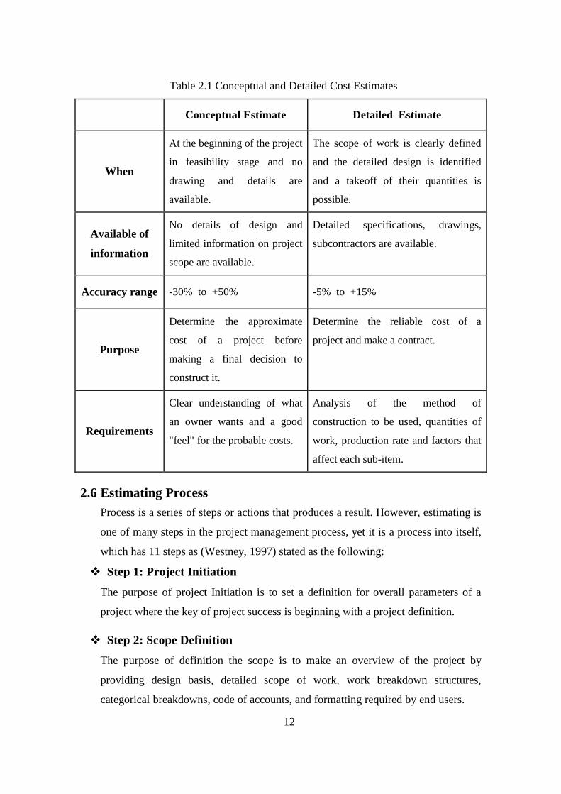
The following Table ‎2.1 summarizes the views of researchers about conceptual and

detailed estimate (Leng, 2005; Choon & Ali, 2008; Al-Thunaian, 1996; Hinze, 1999;

Humphreys, 2004; Abdal-Hadi, 2010):

12

Table ‎2.1 Conceptual and Detailed Cost Estimates

Conceptual Estimate Detailed Estimate

When

At the beginning of the project

in feasibility stage and no

drawing and details are

available.

The scope of work is clearly defined

and the detailed design is identified

and a takeoff of their quantities is

possible.

Available of

information

No details of design and

limited information on project

scope are available.

Detailed specifications, drawings,

subcontractors are available.

Accuracy range -30% to +50% -5% to +15%

Purpose

Determine the approximate

cost of a project before

making a final decision to

construct it.

Determine the reliable cost of a

project and make a contract.

Requirements

Clear understanding of what

an owner wants and a good

"feel" for the probable costs.

Analysis of the method of

construction to be used, quantities of

work, production rate and factors that

affect each sub-item.

Estimating Process 2.6

Process is a series of steps or actions that produces a result. However, estimating is

one of many steps in the project management process, yet it is a process into itself,

which has 11 steps as (Westney, 1997) stated as the following:

Step 1: Project Initiation

The purpose of project Initiation is to set a definition for overall parameters of a

project where the key of project success is beginning with a project definition.

Step 2: Scope Definition

The purpose of definition the scope is to make an overview of the project by

providing design basis, detailed scope of work, work breakdown structures,

categorical breakdowns, code of accounts, and formatting required by end users.

13

Step 3: Pre-Estimate Planning

It reduces the total effort that can be spent to develop the estimate, it also provides

associated information to other project participants.

Step 4: Quantity Take-Offs and Item Descriptions

Estimate items must be listed and quantity take-offs start with estimate detail

sheets for all work items in the project (Popescu, et al., 2003).

Step 5: Data Sources and Costs

There are numerous sources that data can be obtained as quotes, histories or

commercially available data sources, or old estimates in the estimating files.

Step 6: Summary and cover sheets

The main purpose of the summary sheet is to state the total estimated cost for the

project by providing a format for summarizing all the project‟s direct costs and

indirect costs. Where;

Direct cost: are mainly the materials, labor, plant, and subcontractor costs involved

in executing the works (Al-Shanti, 2003).

Indirect cost: are costs other than direct costs of construction activities, and they

are not physically traceable (Marjuki, 2006).

Step 7: Documentation and checking

Documentation and checking is essential for verifying that calculations are valid.

Step 8: Management review

Management plays a key role in reviewing the estimate because they are usually

responsible for oversight of estimate preparation and they typically have the insight

and experience to know “what could go wrong”.

Step 9: Estimate issue and filing

The estimate numbering systems need to be well thought out to be easyfor retrieval

and comfortable for users.

Step 10: Cost feedback continual improvement

This is step is very important to develop the accuracy of the estimating data,

estimator performance, and project histories.

14

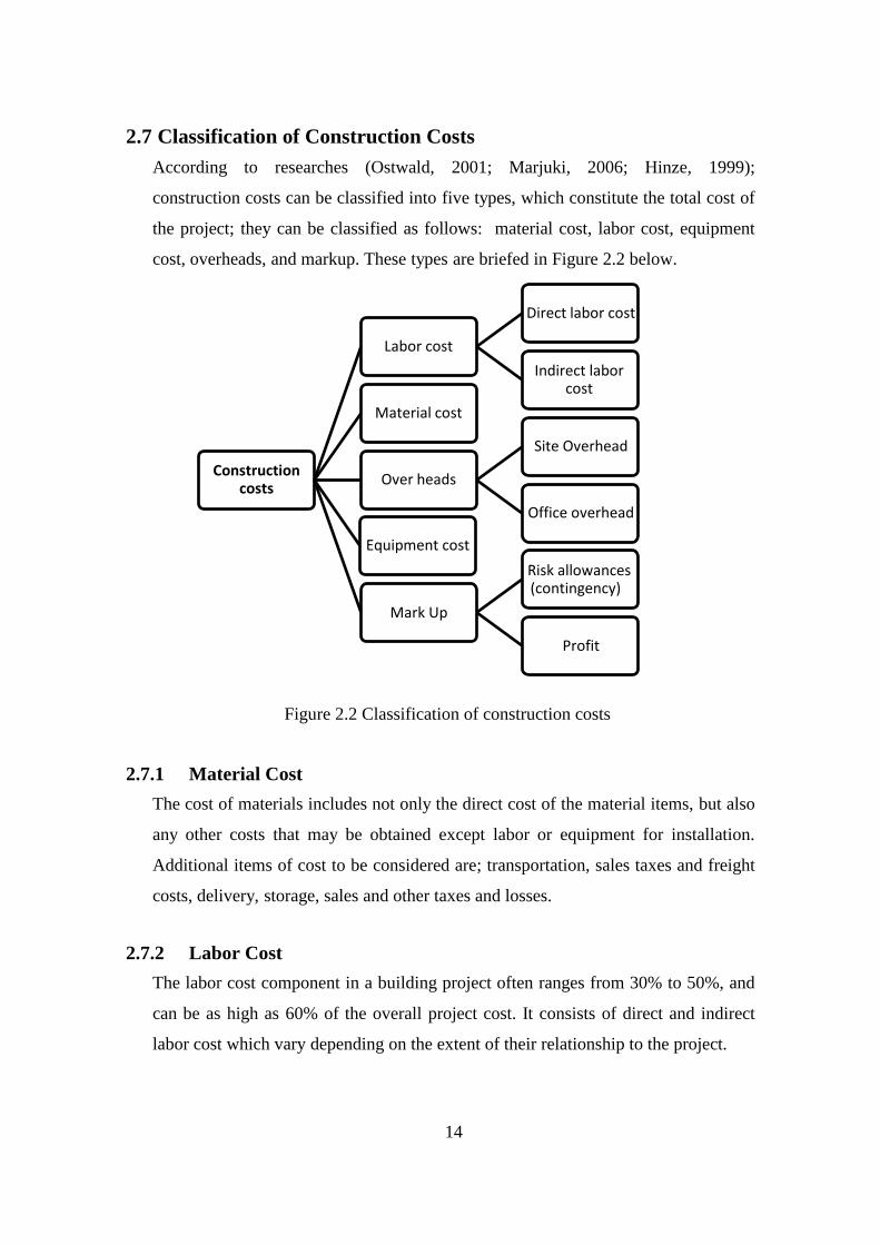
Classification of Construction Costs 2.7

According to researches (Ostwald, 2001; Marjuki, 2006; Hinze, 1999);

construction costs can be classified into five types, which constitute the total cost of

the project; they can be classified as follows: material cost, labor cost, equipment

cost, overheads, and markup. These types are briefed in Figure ‎2.2 below.

2.7.1 Material Cost

The cost of materials includes not only the direct cost of the material items, but also

any other costs that may be obtained except labor or equipment for installation.

Additional items of cost to be considered are; transportation, sales taxes and freight

costs, delivery, storage, sales and other taxes and losses.

2.7.2 Labor Cost

The labor cost component in a building project often ranges from 30% to 50%, and

can be as high as 60% of the overall project cost. It consists of direct and indirect

labor cost which vary depending on the extent of their relationship to the project.

Construction costs

Labor cost

Direct labor cost

Indirect labor cost

Material cost

Over heads

Site Overhead

Office overhead

Equipment cost

Mark Up

Risk allowances (contingency)

Profit

Figure ‎2.2 Classification of construction costs

15

2.7.3 Equipment Costs

Equipments can be classified as specific use or general use as following:

I. Specific use equipment:

This equipment is only for specific construction operations and it is removed from

the jobsite soon after the task is completed.

II. General use equipment:

General use equipment has shared utilization by all subcontractors on the

construction site and it is not associated with any particular work item or items.

2.7.4 Overheads

Overheads cost are construction costs of any kind that cannot be attributed to any

specific item of work. In general, Overheads are a significant item of expense and

will generally run from (5% to 15 %) of the total project cost, depending

somewhat on where certain project costs are included in the cost estimate.

2.7.5 Markup

In construction industry, markup is defined as the amount added to the estimated

direct cost and estimated job into overhead cost to recover the firm‟s main office

allocated overhead (general overhead) and desired profit. In general, markup can

be classified into two main categories as:

I. Risk allowance (Contingency)

The contingency is a specific provision; it must be included to account for

unforeseen elements of cost (Ahuja et al. cited in (Al-Shanti, 2003)).

Ostwald (2001) stated that contingency is the amount of money added to an

estimate to cover unforeseen needs of the project, construction difficulties, or

estimating accuracy. In addition, he quoted the main items that make many chief

estimators or contractor to executives add a contingency to the estimate to cover

one or possibly more of the following:

Unpredictable price escalation for materials, labor, and installed equipment

for projects with an estimated duration greater than 12 months;

Project complexity;

Incomplete working drawings at the time detail estimate is performed;

16

Incomplete design in the fast-track or design-build contracting approach;

Soft spots in the detail estimate due to possible estimating errors, to balance

an estimate that is biased low;

Abnormal construction methods and startup requirements;

Estimator personal concerns regarding project, unusual construction risk,

and difficulties to build; and

Unforeseen safety and environmental requirements.

Accordingly, contingency is not a potential profit and it should not be treated as

an allowance. It includes risk and uncertainty but explicitly excludes changes in

the project scope (change orders).

II. Profit

The amount of profit is generally computed as a percentage of the contract, or in

some cases, as a percentage of each item in the contract. Generally, the

magnitude of desired profit must be decided by the owner for each individual

bid, depending on local market conditions, competition, and the contractor‟s

need for new work.

Methods of Cost Estimation 2.8

Cost estimation methods can be categorized into several techniques as;

2.8.1 Quantitative and Qualitative Technique

Qualitative approaches rely on expert judgment or heuristic rules, and quantitative

approaches classified into statistical models, analogous models and generative-

analytical models (Duran, et al., 2009; Caputo & Pelagagge, 2008). Quantitative

approach has been divided into three main techniques according to (Cavalieri, et al.,

2004).

(a) Analogy-Based Techniques

This kind of techniques allows obtaining a rough but reliable estimation of the

future costs. It based on the definition and analysis of the degree of similarity

between the new project and another one. The underlying concept is to derive the

estimation from actual information. However, many problems exist in the

application of this approach, such as:

17

The difficulties in the measure of the concept of „„degree of similarity‟‟.

The difficulty of incorporating in this parameter the effect of technological

progress and of context factors.

(b) Parametric Models

According to these techniques, the cost is expressed as an analytical function of a

set of variables. These usually consist in some features of the project

(performances, type of materials used), which are supposed to influence mainly the

final cost of the project (known also as „„cost drivers‟‟). Commonly, these

analytical functions are named „„Cost Estimation Relationships‟‟ (CER), and are

built through the application of statistical methodologies.

(c) Engineering Approaches

In this case, the estimation is based on the detailed analysis and features of the

project. The estimated cost of the project is calculated in a very analytical way, as

the sum of its elementary components, comprised by the value of the resources used

in each step of the project process (raw materials, labor, equipment, etc.).

Due to this more details, the engineering approach can be used only when all the

characteristics of the project process are well defined.

2.8.2 Preliminary and Detailed Techniques

For both preliminary and detailed technique its own methods, especially since

preliminary methods are less numeric than detailed methods. However, most of

researchers seek for s perfect preliminary method that gives good results. Ostwald

(2001) outlined commonly methods that are divided into two sets qualitative

preliminary methods as opinion, conference, and comparison similarity or analogy

and quantitative preliminary methods as unit method, unit quantity, linear

regression...etc.

2.8.3 Traditional and Artificial Intelligence Based Techniques

In fact, most of earlier traditional methods fall into one of the following categories;

Time referenced cost indices, cost capacity factors, component ratio, and parameter

costs. However, many researches addressed these traditional parametric methods as

(Mahamid & Bruland, 2010) and (Kim, et al., 2004),.. etc.

18

Recently new approaches were introduced in the last years based on the concept of

parametric models that based on computerized techniques such as artificial

intelligence, which attempt to simulate human intelligence such as Artificial Neural

Network (ANN), Fuzzy logic, etc., where it stills under research and development

especially in construction sector.

Artificial Neural Networks (ANNs) 2.9

Artificial Neural Networks (ANNs) as the name suggests are inspired by the

biology of a brain‟s neuron. Human brain can perform a wide range of complex

tasks in a relatively easier way as compared to computers. Therefore, researchers

were looking for ways in which human intelligence can be incorporated into

machines so that they can also perform certain complex tasks easily. ANNs

resembles the human brain in two aspects; the knowledge acquired by the

network through a learning process, and inter-neuron connection strengths known

as synaptic weights used to store the knowledge (Edara, 2003).

In early stage of a project, there is a limited availability of information, and limited

application of traditional methods that require a precise knowledge of all

parameters and their interrelations. Therefore, the researchers have worked to

develop cost estimate system that maximize the practical value of limited

information available in order to improve cost estimate accuracy and reliability by

developing many cost estimation models. In recent years, new approaches of

artificial intelligence have been grown in popularity that are applicable to cost

estimation problems related to expert systems, case-based reasoning (CBR),

artificial neural networks (ANNs), fuzzy logic (FL), genetic algorithms (GAs), ..etc.

(Cheng, et al., 2010).

ANNs is one of these new approaches that is able to perform tasks involving

incomplete data sets, fuzzy or incomplete information and for highly complex and

ill-defined problems. ANNs can learn from examples and able to deal with non-

linear problems. One of the distinct characteristics of ANN is its ability to learn

from experience and examples and then to adapt to changing situations. It has a

natural propensity for storing experiential knowledge and making it available for

use (Doğan, 2005).

19

According to Kim, et al., (2004), ANN is an applicable alternative for predicting

construction costs because it can find a good cost estimating relationship that

mathematically describes the cost of a system as a function of the variables that

have the most effect on the cost of that system. Weckman, et al., (2010) see that,

the major benefit of ANN is its ability to understand and simulate complex

functions including those dimensions, attributes, and other factors.

In concerning of the structure of ANNs, they are inspired to the human brain

functionality and structure which consist of a set of neurons, grouped in one or

more hidden layers connected by means of synapse connections. The connections

between neurons are called synapses and could have different levels of electrical

conductivity, which is referred to as the weight of the connection. This network of

neurons and synapses stores the knowledge in a „„distributed‟‟ manner: the

information is coded as an electrical impulse in the neurons and is stored by

changing the weight (i.e. the conductivity) of the connections (Cavalieri, et al.,

2004).

2.9.1 Historical Background of ANNs

The applications of ANN in construction management go back to the early 1980‟s.

These applications of ANN cover a very wide area of construction issues (ElSawy,

et al., 2011). The early attempts to embed ANN techniques within the cost

estimation area were conductedby Shtub and Zimerman (1993) who developed

models for estimating the cost of assembly systems.Ehrlenspiel, Schaal (1992),

Becker and Prischmann (1993) who developed cost models using curve-fitting

multi-layer networks, where performance evaluation and a systematic comparison

with conventional methods were not undertaken through theirwork (Wang, 2007).

Internationally, neural network models have been developed to assist the

construction managers or contractors in many crucial construction decisions.

Some of these models were designed for cost estimation, decision making,

predicting the percentage of mark up, predicting production rate …etc (ElSawy, et

al., 2011).

20

2.9.2 Definition of ANN

There is no universally accepted definition of Neural Network (NN), but most of

definitions are similar to some extent with each other, as such, Swingler (1996)

defined neural networks as "statistical models of real world systems which are built

by tuning a set of parameters. These parameters, known as weights, describe a

model which forms a mapping from a set of given values known as inputs to an

associated set of values the outputs".

Bouabaz and Hamami (2008) agreed with Haykin (1998) that artificial neural

networks are inspired from the biological structure of the human brain, which

acquires knowledge through a learning process, and an interneuron connection

strengths known as synaptic weights are used to store the knowledge. However, the

word "neural" is used because of historical reasons since most of the earlier

researchers came from biological or psychological backgrounds, not engineering or

computer science.

Kim, et al., (2004) defined Neural Network (NN) as a computer system that

simulates the learning process of the human brain that can be applied in many

industrial areas, including construction industries.

2.9.3 Neural Networks versus Conventional Computers

The main difference between the neural network and conventional computers lies in

the way they tackle the problem of pattern recognition (Minin, cited in (Aneja,

2011)). Neural networks take a different approach to problem solving than that of

conventional computers. Conventional computers use an algorithmic approach i.e.

the computer processing is sequential-one task, then the next, then the next, and so

on. Unless the specific steps that the computer needs to follow are known, the

computer cannot solve the problem. In comparison, ANNs are not sequential or

necessarily deterministic. There are no complex central processors, rather there are

many simple ones which generally do nothing more than take the weighted sum of

their inputs from other processors. Another fundamental difference between

conventional computers and artificial neural networks is the way in which they

function. Conventional computers use a cognitive approach to problem solving;

21

where they must learn only by doing different sequences or steps in an algorithm

and the problem must be known and stated in small unambiguous instructions.

These instructions are then converted to a high level language program like C++ or

Java,.. etc., and then into machine code that the computer can understand.

Nevertheless, in artificial neural networks the network is composed of large number

of highly interconnected processing elements (neurons) working in parallel to solve

a specific problem, and they can learn by example. They cannot be programmed to

perform a specific task.

In summary, conventional algorithmic computers and neural networks are not in

competition but complement each other. There are tasks, which are more suited to

an algorithmic approach like arithmetic operations, and tasks that are more suited

to neural networks. Even more, a large number of tasks, require systems that use a

combination of the two approaches where normally a conventional computer is

used to supervise the neural network in order to perform at maximum efficiency

(Kshirsagar & Rathod, 2012).

2.9.4 Neural Network Structure

Neural network structure plays a significant role in model accuracy. (Dindar

,2004). However, there are no applicable rules for the optimal setting of control

variables and topologies (Caputo & Pelagagge, 2008).

Otherwise, Generalization and over fitting is directly related to the architecture

used in the neural network to model the data, since training iterations and the

number of hidden units are key elements during the training of the network, and

adjusting these elements could lead to great improvements in the networks

modeling capability (Dindar, 2004).

Bouabaz & Hamami, (2008), demonstrated that there is a number of factors for

selecting the neural network structure and rules, such as the nature of the problem,

data characteristics, complexity of data and the number of sample data.

22

The network architecture refers to the number of hidden layers and the number of

nodes within each hidden layer. As a matter of fact, there are two questions in

designing a neural network that have no specific answers because they are mainly

depend on application; the first is the required data to train a network, and the best

number of hidden layers and nodes to be used. Generally, the more data and the

fewer hidden layers and hidden nodes that can be used, is the better. There is a

subtle relationship between the number of facts and the number of hidden

layers/nodes. Having too few facts or too many hidden layers/nodes can cause the

network to "Memorize". When this happens, it performs well during training but

tests poorly (ElSawy, et al., 2011).

As a rule of thumb, determining the number of hidden layer/neurons is one of the

main drawbacks of NNs, because there is no specific rule and it requires many

trial and error processes while considerable time must be spent (Kim, et al., 2004).

Hegazy & Moselhi, (1995) stated that one hidden layer with a number of hidden

neurons as 0.5 m, 0.75m, m, or 2m+1, where m is the number of input neurons, is

suitable for most applications.

The main building elements of ANNs are neurons or nodes and the links

connecting between them. Each link has a weight parameter associated with it.

These nodes or neurons are assorted into three categories, which are input, output,

and hidden neurons. Each neuron receives stimulus from the neighboring neurons

connected to it, processes the information and produces an output. Neurons that

receive stimuli from outside the network (i.e., not from neurons of the network)

are called input neurons. Neurons whose outputs are used externally are called

output neurons. Neurons that receive stimuli from other neurons and whose output

is a stimulus for other neurons in the neural network are known as hidden neurons.

There are different ways in which information can be processed by a neuron, and

different ways of connecting the neurons to one another. In general, different

neural network structures can be constructed by using different neurons or nodes

and by the specific manner in which they are connected (Cengiz, et al., 2005).

23

Figure ‎2.3 displays the above structure of ANN, which consists of three basic

layers, input, hidden and output layer. Each one contains several neurons except

output layer; it contains one neuron that represents the output of training process.

For hidden neurons, Figure ‎2.4 presents the schematic diagram that shows

weight's summation part and transfer function part inside these neurons.

2.9.5 Terminology Used In Artificial Neural Network

Weight: In an artificial neural network, A weight is a parameter associated

with a connection from one neuron, M, to another neuron N. It determines how

much notice the neuron N pays to the activation it receives from neuron M (Al-

Najjar, 2005).

Figure ‎2.4 Schematic diagram of processing element (Mohaghegh, 2000)

Figure ‎2.3 Artificial Neural Network structure

24

Learning algorithm: Is a systematic procedure for adjusting the weights in the

network to achieve a desired input/output relationship (Al-Najjar, 2005). The

goal of the learning process is to minimize the error between the desired output

and the actual output produced by the network. After learning process, the

neural network has learned to produce an output that closely matches to the

desired output (Jitendra, et al., 2011).The learning algorithms of neural

networks are divided into three categories;

- Reinforcement learning method: The network is not provided with the

output but it is informed if the output is a good fit or not (Karna & Breen,

1989).

- Unsupervised learning method: The target output is not presented to

the network. Thus, the network follows a self-supervised method and

makes no use of external influences for synaptic weight modification

(Jitendra, et al., 2011).

- Supervised learning method: The network is provided with number of

layers, the number of neurons per layer of the network and the type of

activation function used, and the synaptic weights, then the network

adjusts the weights after comparing the results from the network with the

output to minimize the error. Moreover, supervised learning method has

several learning algorithms as Back-propagation Learning rule, Gradient

Descent Learning, Delta Rule (Jitendra, et al., 2011). Where Back-

propagation Learning rule, which is adopted in this research, is the most

common learning method, and it has various algorithms like Levenberg-

Marquardt and Momentum for backpropagation algorithm (Principe, et

al., 2010).

Activation Functions: Activated functions experimentally change based on

the placed independent variables in model and expected outputs (Attal,

2010).The activation function performs a mathematical operation on the signal

output. Depending upon the type of input data and the output required (Kriesel,

2005). Over the years, the researchers tried several functions to convert the

input into output, various mathematical functions have been used as activation

25

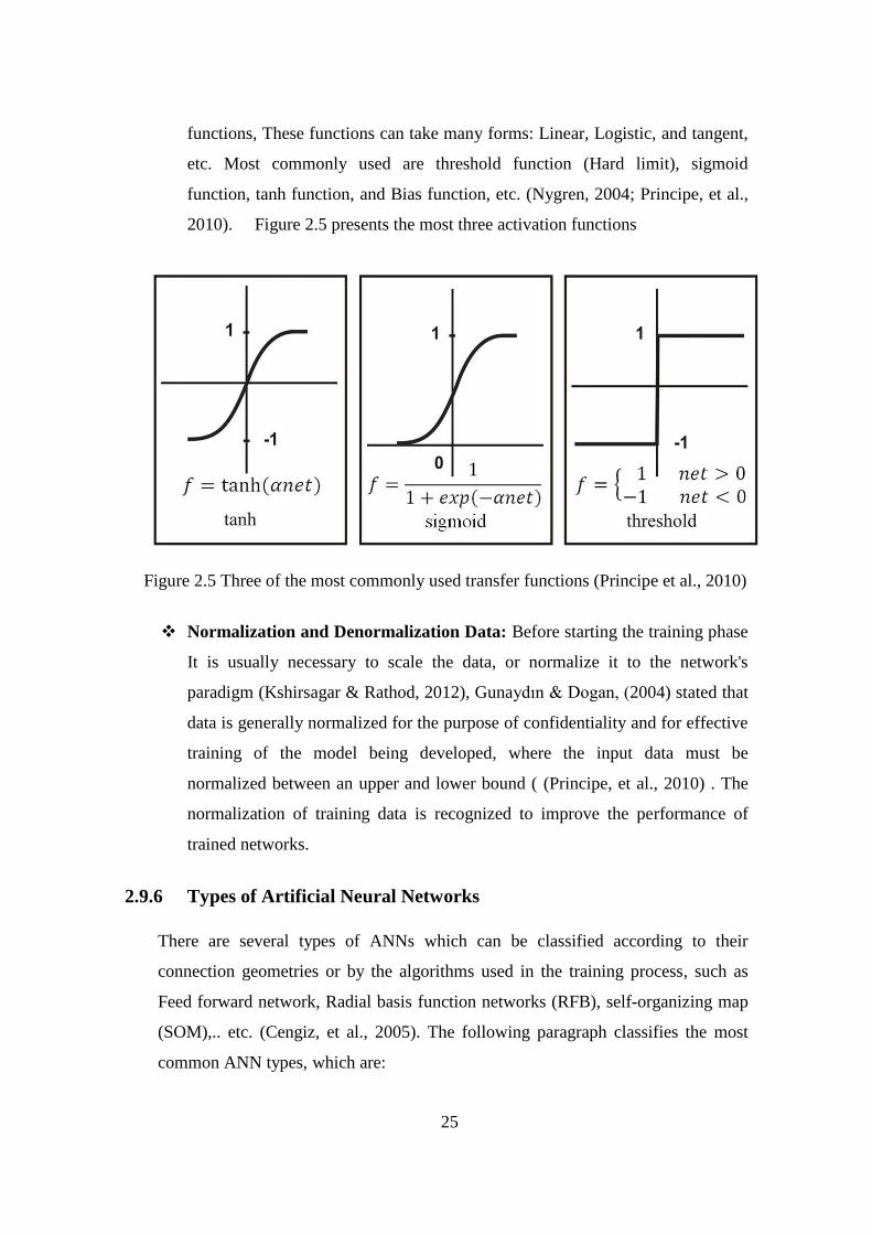
functions, These functions can take many forms: Linear, Logistic, and tangent,

etc. Most commonly used are threshold function (Hard limit), sigmoid

function, tanh function, and Bias function, etc. (Nygren, 2004; Principe, et al.,

2010). Figure ‎2.5 presents the most three activation functions

Figure ‎2.5 Three of the most commonly used transfer functions (Principe et al., 2010)

Normalization and Denormalization Data: Before starting the training phase

It is usually necessary to scale the data, or normalize it to the network's

paradigm (Kshirsagar & Rathod, 2012), Gunaydın & Dogan, (2004) stated that

data is generally normalized for the purpose of confidentiality and for effective

training of the model being developed, where the input data must be

normalized between an upper and lower bound ( (Principe, et al., 2010) . The

normalization of training data is recognized to improve the performance of

trained networks.

2.9.6 Types of Artificial Neural Networks

There are several types of ANNs which can be classified according to their

connection geometries or by the algorithms used in the training process, such as

Feed forward network, Radial basis function networks (RFB), self-organizing map

(SOM),.. etc. (Cengiz, et al., 2005). The following paragraph classifies the most

common ANN types, which are:

mk:@MSITStore:E:/خاص/master/رسالة%20الماجستير/Hassn%20ANN/References/NeuroSolution%20Help/neurosolutions.chm::/COMPONENTS/HID_NSInput.htm

26

Single-Layer Feed Forward Networks

It is the simplest form of a layered network, which consists of a single layer of

weights, where the inputs are directly connected to the outputs by series of

weights. Such a network is called a single-layer network, with the designation

"single layer" referring to the output layer of computation nodes (neurons). The

input layer of source nodes is not counted because no computation is performed

there (Al-Najjar, 2005). Figure ‎2.6 shows the single layer feed forward network.

Feed Forward Network

In this network, the information moves just in one direction, forward, from the

input nodes, through the hidden nodes and to the output nodes. There are no cycles

or loops in the network (Kshirsagar & Rathod, 2012). Feedforward networks can

be classified into several types as Multi-Layer Preceptron, General FeedForward

(GFF), etc., the most common types are MLP and GFF networks (Pawar, 2007).

Multilayer Perceptron (MLP)

The most popular type of neural network in use currently is multilayer perceptron

(MLP) which is commonly used in regression and classification problems. They

are capable of modeling many functions but require a large amount of time,

epochs, and nodes (Weckman, et al., 2010).

Figure ‎2.6 Single layer feed forward network (Al-Najjar, 2005)

27

In (MLP), neurons are organized in several layers: the first is the input layer (fed

by a pattern of data), while the last is the output layer (which provides the answer

to the presented pattern). Between input and output layers there is one or more

hidden layers which are comprised of the nodes chosen in the design phase. Each

node of these takes the input values, associated weights, and runs them through the

chosen function. The chosen function affects how and how well the network is

able to learn. The node then uses a transfer function to produce a weight-

associated output. The hidden node values and weights are run through the output

node (layer) algorithm, and a final output value is calculated (Dowler, 2008). See

Figure ‎2.7

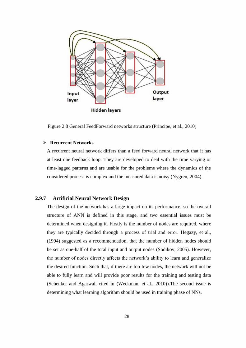
General FeedForward (GFF)

GFF networks are a special case of MLP such that connections can jump over one

or more layers, The GFF networks often solve the problem much more efficiently.

A classic example of this is the two-spiral problem. Without describing the

problem, it suffices to say that a standard MLP requires hundreds of times more

epochs of training than the generalized feedforward (for the same size

network).(Principe, et al., 2010). See Figure ‎2.8

Figure ‎2.7 Multilayer Perceptron (Christian, et al., 2000)

28

Recurrent Networks

A recurrent neural network differs than a feed forward neural network that it has

at least one feedback loop. They are developed to deal with the time varying or

time-lagged patterns and are usable for the problems where the dynamics of the

considered process is complex and the measured data is noisy (Nygren, 2004).

2.9.7 Artificial Neural Network Design

The design of the network has a large impact on its performance, so the overall

structure of ANN is defined in this stage, and two essential issues must be

determined when designing it. Firstly is the number of nodes are required, where

they are typically decided through a process of trial and error. Hegazy, et al.,

(1994) suggested as a recommendation, that the number of hidden nodes should

be set as one-half of the total input and output nodes (Sodikov, 2005). However,

the number of nodes directly affects the network‟s ability to learn and generalize

the desired function. Such that, if there are too few nodes, the network will not be

able to fully learn and will provide poor results for the training and testing data

(Schenker and Agarwal, cited in (Weckman, et al., 2010)).The second issue is

determining what learning algorithm should be used in training phase of NNs.

Figure ‎2.8 General FeedForward networks structure (Principe, et al., 2010)

29

2.9.8 Training of Neural Network

The objective of training a neural network is to adjust the neural network weights to

bring its output closer to the desired output, where the weights after training contain

meaningful information, whereas before training, they are random and have no

meaning.

This process of changing or adapting the connection weights in some orderly fashion

using a suitable learning method is referred to as the learning rule of the network

(Doğan, 2005).

The first step in training process is to initialize the weight of parameters that randomly

assigned to the links between nodes. The output of the neural network is compared with

desired values, and an error is calculated by learning algorithm then the weights

associated with each link are adjusted in an attempt to minimize the network‟s mean

square error.The input values are run through the network with the adjusted weights and

the process restarts from the beginning. The process is repeated for the predetermined

number of epochs. An epoch represents one cycle of the training process (Dowler,

2008). When the training reaches a satisfactory level, the network holds the weights

constant and uses the trained network to make decisions, or define associations in new

input data sets not used to train it (Doğan, 2005).

As mentioned earlier, there are several training algorithms to be chosen for training

process, one of the most common and powerful algorithm that is adopted in this study is

Back propagation algorithm which belongs to the realm of supervised learning

(Gunaydın & Dogan, 2004). On one hand, Back propagation was invented in 1969 to

learn a multilayer network for a given set of input patterns with known classifications. It

tries to improve the performance of the neural network by reducing the total error

through changing the weights along its gradient (Jitendra, et al., 2011). The error can be

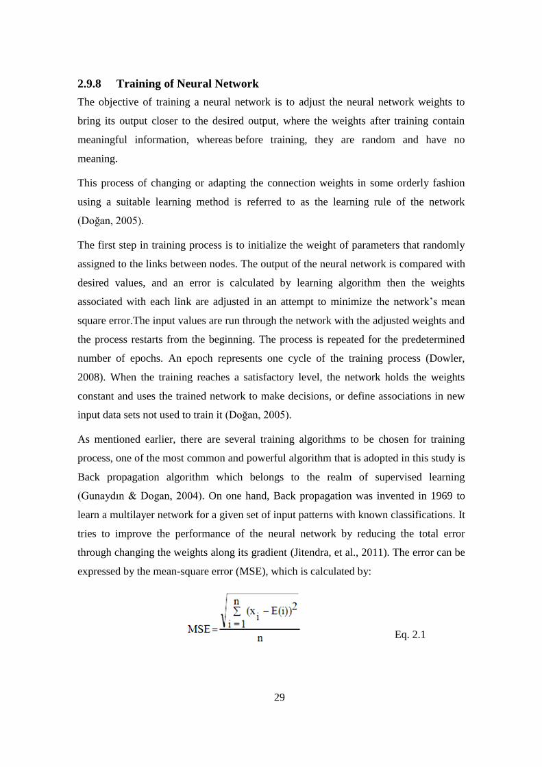
expressed by the mean-square error (MSE), which is calculated by:

Eq. 2.1

30

Where: - n is the number examples to be evaluated in the training set,

- xi is the network output (target) related to the example (i=1,2,…,n),

- and E(i) is the desired output.

As the error converges to zero, the output patterns computed by the ANN perfectly

match the expected values, and the network is well trained (Dogan, 2005).The algorithm

involves two phases, Forward phase to compute the output and the backward phase to

perform modifications in the backward direction (Jitendra, et al., 2011).

These two phases compose on cycle, where each training cycle is called an epoch, and

the weights are updated in each cycle. Each training cycle stops when one of the

following three conditions is met (Weckman, et al., 2010):

1) The maximum number of epochs was reached,

2) The cross validation error started increasing, or

3) Very large number of epochs without improvement in error are reached.

Eventually, the network's weights are continuously adjusted until the error in the

calculated outputs converges to an acceptable level or stopping the training process if

one of previous condition is reached.

2.9.9 Cross-validation of Neural Network

A simple method to compare the performance of neural networks is to test the errors of

the networks using a separate validation / test data set. Basically, the available data is

always divided into three parts prior to the training including training data, cross-

validation data, and testing data. The cross-validation data is used during the training

but for monitoring not to train the network, instead to check the learning of the network

during the training; and the testing data is used to validate the training network after

finishing training process (Edara, 2003).

Cross validation uses its own data set to monitor the neural network‟s ability to produce

generalized cost estimates; this is done by training many networks on a training set and

comparing the errors of the networks on the validation set. The networks that performed

best on the validation data set are then selected (Dindar, 2004). The network continues

to learn as the error for the cross validation and the training data set continue to

31

decrease. Once the error for the cross validation data set starts to increase, the training

stops and the weight values that provided the lowest error for the cross validation data

set are considered the best. The training set error value may continue to decrease once

the cross validation error starts to rise. At this point, the network is over-fitting and

memorizing the training data. If cross validation is not used, then a testing data set is

critical to prove that memorization and over-fitting is not occurring (Weckman, et al.,

2010), (Dowler, 2008).

The next Figure ‎2.9 illustrates the earlier mechanism of cross validation process that it

appears the point at which the training process stops due to start increasing error curve

of cross validation set.

2.9.10 Testing of Neural Network

Testing the network is essentially the same as training (ElSawy, et al., 2011). The

testing set is critical to confirm that the network has not simply memorized a given set

of data but has learned the general patterns involved within an application (Kshirsagar

& Rathod, 2012).

The testing data is totally a different set of data that the network is unaware of; after

finishing the training process testing data is used for validation and generalization of the

trained network. If the network is able to generalize rather precisely the output for this

Figure ‎2.9 Typical error graph for NN using cross validation (Weckman et al., 2010)

32

testing data, then it means that the neural network is able to predict the output correctly

for new data and hence the network is validated. Moreover, the amount of data that is to

be used for training and testing purposes is depending on the availability of the data, but

in general the training data is 2/3rd of the full data and the remaining is used for testing

purposes. The cross-validation data can be 1/10th of the training data (Edara, 2003).

2.9.11 Performance Measures of ANN model

The most common approaches have been utilized to determine the estimation accuracy

in testing phase are:

- Mean Absolute Error (MAE)

- Mean Absolute Percentage Error (MAPE)

- Total Mean Absolute Percentage Error (Total MAPE)

- Correlation Coefficient (r)

I. Mean Absolute Error (MAE):

It is one of many ways to quantify the difference between an estimated and the

actual value of the projects being estimated. According to Willmott & Matsuura,

(2005) the MAE is relatively simple; It involves summing the magnitudes

(absolute values) of the errors to obtain the „total error‟ and then dividing the total

error by n, it can be defined by the following formula:

∑ ∑ | |

Eq. ‎2.2

Where: P = number of output PEs.

N = number of exemplars in the data set.

dyij= denormalized network output for exemplar i at PE j.

ddij= denormalized desired output for exemplar i at PE j.

II. Mean Absolute Percentage Error (MAPE):

The mean absolute error is a quantity used to measure how close forecasts or

predictions are to the eventual outcomes, according to Principe, et al., (2010) The

MAPE is defined by the following formula:;

∑ ∑

| |

Eq. 2.3

33

Where: P = number of output PEs.

N = number of exemplars in the data set.

dyi j= denormalized network output for exemplar i at PE j.

ddi j= denormalized desired output for exemplar i at PE j.

Note that this value can easily be misleading. For example, say that your output data

is in the range of 0 to 100. For one exemplar your desired output is 0.1 and your

actual output is 0.2. Even though the two values are quite close, the percent error for

this exemplar is 100 (Principe, et al., 2010).

III. Correlation Coefficient (r):

According to Principe et al., (2010) the size of the mean square error (MSE) can

be used to determine how well the network output fits the desired output, but it

doesn't necessarily reflect whether the two sets of data move in the same direction.

For instance, by simply scaling the network output, we can change the MSE

without changing the directionality of the data. The correlation coefficient (r)

solves this problem.

By definition, the correlation coefficient between a network output x and a desired

output d is:

∑ ( )( )

√∑ ( )

√∑ ( )

Eq. ‎2.4

The correlation coefficient is confined to the range [-1,1]. When r =1 there is a

perfect positive linear correlation between x and d, that is mean x and d vary by the

same amount. When r=-1, there is a perfectly linear negative correlation between x

and d, that means they vary in opposite ways (when x increases, d decreases by the

same amount). When r =0 there is no correlation between x and d, i.e. the variables

are called uncorrelated. Intermediate values describe partial correlations. For

example a correlation coefficient of 0.88 means that the fit of the model to the data

is reasonably good (Principe, et al., 2010).

34

IV. Total Mean Absolute Percentage Error (Total MAPE):

According to Hegazy & Ayed, (1998); the total MAPE methdology is defined by

determinig the total MAPE. Training phase were represented fifty percent of the

total MAPE likewise the test set is equal the remaining fifty percent.

( ) ( )⁄

Eq. ‎2.5

Where: MAPETr = Mean absolute percentage error for training data set.

NTr = number of exemplars in the training data set.

MAPEC.V = Mean absolute percentage error for cross validation data set.

NTr = number of exemplars in the cross validation training data set.

MAPETest = Mean absolute percentage error for test data set.

2.9.12 Sensitivity Analysis of ANN model

Once the optimum Neural Network model has been selected as described early, Sensitivity

analysis was run on the best model to evaluate the influence of each input parameters to

output variable. This provides a feedback as to which input parameters are the most

significant, it allows the user to see how the input affects the output over a range of values if all

other inputs remain constant. As well, it will reduce the size of the network by removing the

less significance factors and in turn the complexity of the model and the training times

(Gunaydın & Dogan, 2004) (Bouabaz & Hamami, 2008). However, the small effect

parameters doesn‟t necessary means should be excluded from the model because these

parameters could enhance the learning capability of the model to achieve the best output

(Arafa & Alqedra, 2011).

Sensitivity analysis was carried out on the best model by using Neurosolution tool, which

was run after fixed the best weights, first started by varying the first input between the

mean ± one standard deviation, while all other inputs are fixed at their respective

means. The concept of calculating the sensitivity analysis of input factors based on

determining the standard deviation of each by using the following formula :

√( )

( ) Eq. ‎2.6

Where x: is the output value.

x: is the mean of the output values.

n: is the number of the outputs in the sample.

35

2.9.13 Neural Network Properties

NNs have some properties, as they are non-parametric and make weaker assumptions.

However, it is able to model interdependencies between input data which will inevitably

occur when considering construction cost significant variables. For example, the model

variables, such as number of floors, gross floor area and number of lifts, will almost

certainly be correlated.

An important property of NNs is their ability to detect hidden relationships among case

data and to apply these relationships to new data. They can be used to classify data

(clustering), to approximate functions (curve), and to extract orthogonal factors

(principle components) from interdependent data. Moreover, NNs are robust; they are

able, within limits, to deal with inexact or missing data. However, the suitability of the

result depends on the type of application and the architecture of the network. Another

property is the robustness of NNs against physical failure of a single component. The

low level of complexity and the small number of training samples allow NNs to run on

a single microcomputer (Bode, 1998).

According to these properties of the NNs; it achieves many pros in estimate cost area

include accuracy, time, and the ability for a person with very little knowledge about the

part or neural networks to produce a good cost estimate once the network has been

trained (Dowler, 2008).

Neural networks can deal more readily with multivariate non-linear relationships

problems. More significantly, these relationships are determined implicitly by the

model, and do not therefore require them to be specified (Harding, et al., 1999).

Al-Najjar, (2005) summarized some advantages of ANN from several researches as the

following:

1- ANN are well suited to model complex problems where the relationship between

the model variables is unknown.

2- Neural networks have the capability of producing correct or nearly correct

outputs when presented with partially incorrect or incomplete inputs.

36

3- ANN do not need any prior knowledge about the nature of the relationship

between the input/output variables, which is one of the benefits that ANN have

compared with most empirical and statistical methods.

4- ANN can always be updated to obtain better results by presenting new training

examples as new data become available.

5- Artificial Neural Networks have the advantage that it gives you the output

without the need to perform any manual work such as using tables, charts, or

equations.

6- It is often faster to use neural networks than a conventional approach.

7- Engineers often deal with incomplete and noisy data which is one area where

ANN are most applicable.

8- ANN can learn and generalize form examples to produce meaningful solutions

to problems.

9- Data presented for training ANN can be theoretical data, experimental data,

empirical data based on good and reliable experience or a combination of these.

Eventually, ANN can solve problems that are too complex for conventional

technologies, and create its own organization or representation of the information that it

receives during the learning time by automated transformation of variables in the

network.

2.9.14 Problems and Challenges

Despite the good performance of Neural Networks in the previous studies essentially in

cost estimation, the process of developing and implementing Neural Networks to

parametric cost estimation has a number of problems associated with it. One of the main

problems is the black box nature of neural networks and their inability to duplicate

results. That is because the initial weights being randomly assigned, By another word, it

is hard to persuade individuals who do not have a broad understanding of the

technology that the neural network is producing a reliable cost estimate because it is

very difficult to recreate a network (Dowler, 2008).

These problems usually highlighted in previous researches as (Kim, et al., 2004) who

stated that NN approach is a black box technique and its knowledge acquisition process

is very time consuming. In addition, Islam, et al., (2009) declared that the most problem

37

of NN is its hidden internal structure and it is very difficult to duplicate even using the same

input variables.

Otherwise, designing the network architecture and setting its parameters is not a

straight-forward approach; it actually requires some trial and error process, and there is

no explicit set of rules to determine whether a given learning algorithm is suitable for a

particular application or not. However, some problems related to back-propagation

algorithm are the speed of convergence, the possibility of ending up in a local minimum

of the error function and requiring optimization of the network training in order to

achieve adequate generalization. In addition, the sample size of data has to be large, so a

large amount of time must be spent in determining the best network architecture and the

network parameters that best fit the application under consideration.

Finally, Neural Networks do not perform well with applications where precise

numerical computations are required, like detailed estimating and cost control (Ayed,

1997).

2.9.15 Application of ANN In Cost Estimation

In general, applications of ANN (Artificial Neural Network) in construction

management go back to the early 1980‟s. These applications cover a very wide area of

construction issues. Neural network models have been developed internationally to

assist the managers or contractors in many crucial construction decisions. Some of these

models were designed for cost estimation, decision making, predicting the percentage of

mark up, predicting production rate …etc. (ElSawy, et al., 2011). However, despite the

large number of researchers who applied neural network approach in various fields of

engineering, but the studies and researches on utilizing neural networks to estimate the

cost of construction projects at various stages of the work are very limited (Arafa &

Alqedra, 2011). The early attempts to embed ANN technique within the cost estimation

area was in (1993) by Shtub and Zimer who developed models for estimating the cost of

assembly systems (Wang, 2007).

http://en.wikipedia.org/wiki/Local_minimum

38

Locally, there is a lack of cost estimation researches based on ANN. According to Al-

Shanti (2003) study; the most of contracting companies are still estimating the projects

manually, and a little use friendly estimating software packages due to a lack of

available qualified personnel in using computer-based estimating systems. Therefore, he

(AL-Shanti) tried to develop a cost estimating system that is familiar with many cost

estimators, and it has been designed to run under Microsoft Excel sheets.

Arafa and Alqedra (2011) developed an ANN model to estimate the cost of building

construction projects at early stages. A database of 71 building projects as collected

from the construction industry of the Gaza Strip was used in a developed ANN model

that had one hidden layer with seven neurons. The results obtained from the trained

models indicated that neural networks reasonably succeeded in predicting the early

stage cost estimation of buildings using basic information of the projects and without

the need for a more detailed design.

Regionally, Elsawy et al. (2011) developed a neural network model to assess the

percentage of site overhead costs for building projects in Egypt, which can assist the

decision makers during the tender analysis process. Fifty-two actual real-life cases of

building projects constructed in Egypt during the seven year period 2002-2009 were

used as training materials. The neural network architecture was presented for the

estimation of the site overhead costs as a percentage from the total project price. The

results of the testing model indicated an accuracy of (80%), as the model wrongly

predicted the percentage of site overhead costs for only one project (20%) from the

testing sample.

Internationally, Kim et al. (2005) applied hybrid models of ANN and Genetic

Algorithm (GA) to estimate the preliminary cost of residential buildings. Data used for

training and performance evaluation were for residential buildings constructed from

1997 to 2000 in Seoul, Korea. They first optimized the parameters of the back-

propagation algorithm using genetic algorithms and then obtained a set of trained

weights for the ANN model using GA. The results of the research revealed that

optimizing each parameter of back-propagation networks using GA is most effective in

39

estimating the preliminary costs of residential buildings. They concluded that GA may

help estimators to overcome the problem of the lack of adequate rules for determining

the parameters of ANN.

Gunaydin and Dogan (2004) developed an ANN model to estimate the cost of a square

meter of the structural system of buildings in early phases of design processes. They

collected cost and design data from 30 projects of 4 to 8 storey residential buildings in

Turkey. The input layer of the trained ANN model comprised eight parameters available

at the early design stage. The trained ANN model was capable of providing accurate

estimates of at least 93% of buildings cost per square meter.

Sonmez (2004) developed conceptual cost models for continuing care retirement

community projects with regression analysis and neural networks. The results obtained

from the models were compared for closeness of fit and prediction performance. He

indicated that while regression analysis requires a decision about the class of relations to

be used in modeling neural network was able to identify the relations between variables

and the project cost. It was also shown that by using regression analysis and neural

network techniques simultaneously, a satisfactory conceptual cost model (which fits the

data adequately and has a reasonable prediction performance) can be achieved.

Emsley et al. (2002) trained neural network cost models using a database of data nearly

300 building projects. They used linear regression techniques as a benchmark for

evaluation of the neural network models..The results showed the ability of neural

networks to model the nonlinearity in the data, where the model was capable of

evaluating the total cost of the construction, and the trained ANN model obtained a

mean absolute percentage error of 16.6 %.

The above researches and many other reviewed by the authors indicated that the

application of artificial neural networks to estimate the early cost of construction

projects is a promising area and more studies should be carried out in this field.

40

Neurosolution 5.07 Application 2.10

Several applications support the establishment of neural networks like SPSS,

MATLAB, etc. In this research, NeuroSolution application was selected. where

NeuroSolutions is the premier neural network simulation environment. As mentioned in

NeuroDimension, Inc., (2012) NeuroSolutions combines a modular, icon-based network

design interface with advanced learning procedures and genetic optimization. Perform

cluster analysis, sales forecasting, sports predictions, medical classification, and much

more with NeuroSolutions, which is:

powerful and flexible: neural network software is the perfect tool for solving

data modeling problems, so it's flexible to build fully customizable neural

networks or choose from numerous pre-built neural network architectures.

Modify hidden layers, the number of processing elements and the learning

algorithm (NeuroDimension, Inc., 2012).

Easy to use: NeuroSolutions is an easy-to-use neural network development tool

for Microsoft Windows and intuitive, it does not require any prior knowledge of

neural networks and is seamlessly integrated with Microsoft Excel and

MATLAB. NeuroSolution also includes neural wizards to ensure both beginners

and advanced users can easily get started. (NeuroDimension, Inc., 2012).

http://www.neurosolutions.com/

41

CHAPTER 3

3 Research Methodology

Introduction 3.1

This chapter discusses the methodology used in this research. The adopted methodology

to accomplish this study used historical data analysis as the base of providing a relation

between the main factors affecting the cost of the building projects to make estimates

for new projects.

This chapter provides the information about the research strategy and design, factors

affecting cost of the building projects, process of data collection and analysis.

Research Strategy 3.2

Research strategy in general means a plan of action which the research objectives can be

questioned, and it can be classified into two types namely, quantitative approach and

qualitative approach (Naoum, 2007).

Qualitative approach seeks to gain insights and to understand people's perceptions, or

opinion towards a particular object. As well, it is used when a limited amount of

knowledge about the topic are available (Naoum, 2007).

Quantitative approach seeks to collect factual data and to study relationship between

facts and how such facts and relationships accord with theories and findings of any

research executed previously (Al-Shanti, 2003).

In this study both qualitative and quantitative approaches were used to get the factual

information of the main factors affecting the cost of building projects in Gaza Strip at

conceptual phase. As well as collecting the data from several resources, by filling a

form for each project, which contains the input factors and the actual cost of the project.

Research Design 3.3

The purpose of this research is to develop a model of ANN to use in estimating cost of

building projects as an alternative technique of traditional approach.

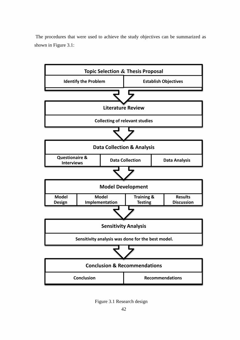
42

Conclusion & Recommendations

Conclusion Recommendations

Sensitivity Analysis

Sensitivity analysis was done for the best model.

Model Development

Model Design

Model Implementation

Training & Testing

Results Discussion

Data Collection & Analysis

Questionaire & Interviews

Data Collection Data Analysis

Literature Review

Collecting of relevant studies

Topic Selection & Thesis Proposal

Identify the Problem Establish Objectives

The procedures that were used to achieve the study objectives can be summarized as

shown in Figure ‎3.1:

Figure ‎3.1 Research design

43

As shown in Figure ‎3.1 the adopted methodology for the completion of this study

follows the following stages:

Topic selection and thesis proposal phase

After selection the topic, problems are defined, objectives are established and, research

plan is developed.

Literature review phase

Previous papers, reports thesis, models, and books, which relevant to cost estimation in

construction industry were reviewed, essentially that studied new approach of cost

estimation like Artificial Neural Networks models.

Data collection phase

A structured questionnaire in addition to expert interviews were used together in this

research, to identify the main parameters affecting cost of building projects in Gaza

Strip. For the need of many data in building the neural network models, many historical

building projects that were done between 2009 and 2012 in Gaza Strip were collected

from municipalities, Government ministries, Engineering institutions, contractors and

consultants in this period especially due to resumption of implementing construction

projects in those years after several Interruption years because of the Israeli blockade.

Model Development phase

After analyzing the data, many models were built and trained with various structures by

using NeuroSolution 5.07. Accordingly, the best model was tested and the sensitivity

analysis have been assessed by variation in the cost of projects.

Conclusion and recommendation phase

In this stage, the content of the thesis was written and the research chapters were

covered. Moreover, the research was summarized in the conclusion section with many

recommendations.

44

CHAPTER 4

4 Data Collection and Results

Factors Affecting Cost of the Building Projects 4.1

In fact, one of the most significant keys in building the neural network model is

identifying the factors that have real impact on the cost of building projects. Depending

on this great importance of selecting these factors, several techniques were adopted

carefully to identify these factors in Gaza Strip building projects; as reviewing literature

studies and bill of quantities (BOQ), surveying a questionnaire, and Delphi technique by

conducting expert interviews.

4.1.1 Questionnaire Analysis

Eighty questionnaires were distributed to various engineering institutions, where, fifty-

seven questionnaires, as a response rate 71% of the total number of questionnaires, have

been correctly answered and submitted. These questionnaires were cleaned, and some of

them were omitted due to incomplete or inaccurate data. More details and analysis are

discussed in this section for the questionnaire results.

I. Study population characteristics

The characteristics of study population comprise of type of company, job title, years of

experience, and the experience in building projects.

a. Type of company

Table ‎4.1 shows that (51%) of respondents were contracting companies, while

(35%) of them were consultant companies, and (14%) were owner of projects.

This indicates that all type of experience are included and the highest percentage

is for who design and estimated the initial cost of projects, and for the companies

which implement and deemed the real cost of projects. However, contracting

companies recorded the highest percentage of respondents due to great number of

contracting companies in comparing with consultant companies in Gaza Strip.

45

Table ‎4.1 Distribution of questionnaire according to company type

No. Description % No.

1 Contracting company 51% 29

2 Consulting company 35% 20

3 Owner (Municipality, ministry,..) 14% 8

The total number of respondents=57 respondent

b. Job title

From Table ‎4.2, it has been found that the survey included most job levels of

engineers, where (46%) of them are project managers, while (39%) site engineer,

and (16%) are owners and others. As shown below, the most level of job title is

project managers who have the whole vision about all of project cost details.

Table ‎4.2 Distribution of questionnaire according to job tittle

c. Years of experience in construction projects

Table ‎4.3 presents the work experience of participants, where (25%) of them have

high experience exceeds than 10 years, while (26%) have 7 to10 year experience,

and (49%) have less 6-year experience. This indicates that the greatest percentage

of respondents have suitable experience in construction field to make them able to

determine the critical factors affect on the cost of projects.

Table ‎4.3 Distribution of questionnaire according to number of experience years

No. Description Percent Frequency

1 Owner of company 7% 4

2 Project manager 46% 26

3 Site engineer 38% 22

4 Others 9% 5

Description Percent Frequency

1 – 3 years 17% 10

4 – 6 years 32% 18

7 – 10 years 26% 15

More than 10 25% 14

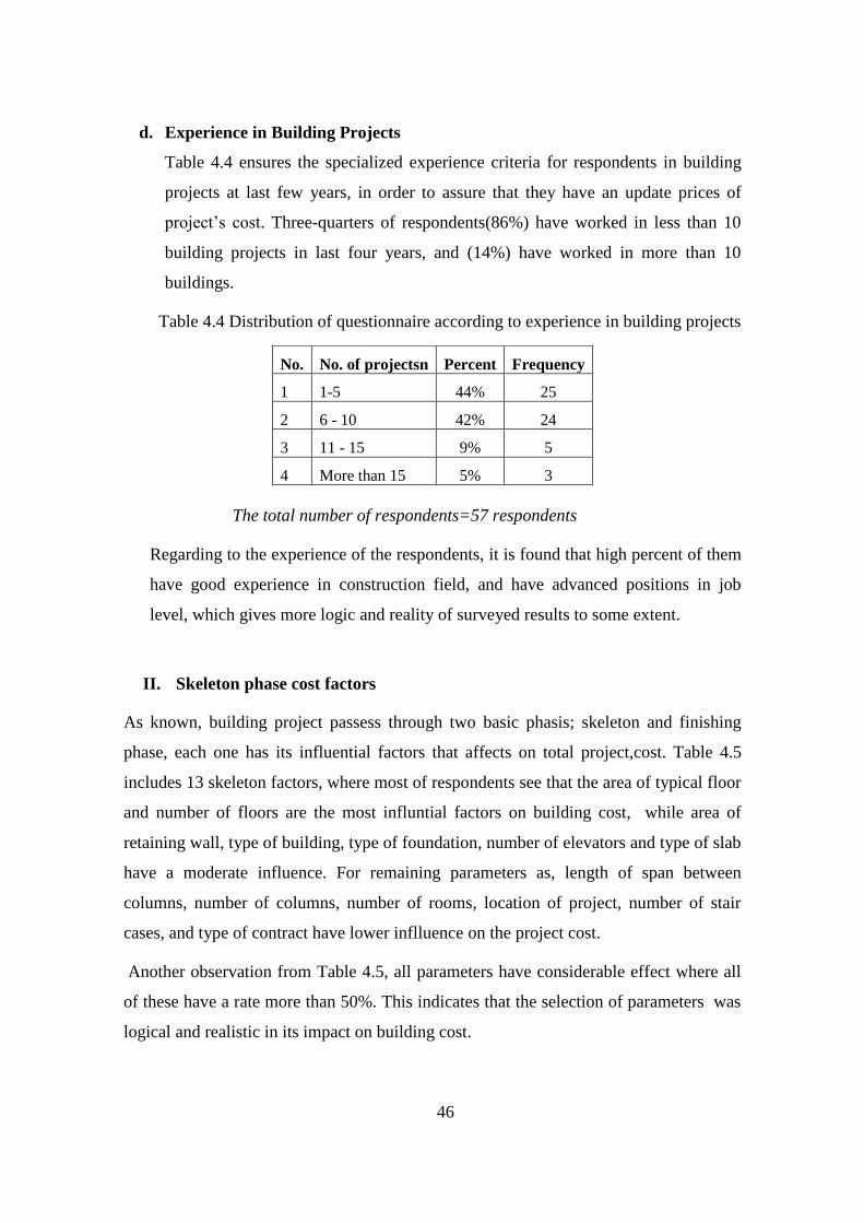
46

d. Experience in Building Projects

Table ‎4.4 ensures the specialized experience criteria for respondents in building

projects at last few years, in order to assure that they have an update prices of

project‟s cost. Three-quarters of respondents(86%) have worked in less than 10

building projects in last four years, and (14%) have worked in more than 10

buildings.

Table ‎4.4 Distribution of questionnaire according to experience in building projects

The total number of respondents=57 respondents

Regarding to the experience of the respondents, it is found that high percent of them

have good experience in construction field, and have advanced positions in job

level, which gives more logic and reality of surveyed results to some extent.

II. Skeleton phase cost factors

As known, building project passess through two basic phasis; skeleton and finishing

phase, each one has its influential factors that affects on total project,cost. Table ‎4.5

includes 13 skeleton factors, where most of respondents see that the area of typical floor

and number of floors are the most influntial factors on building cost, while area of

retaining wall, type of building, type of foundation, number of elevators and type of slab

have a moderate influence. For remaining parameters as, length of span between

columns, number of columns, number of rooms, location of project, number of stair

cases, and type of contract have lower inflluence on the project cost.

Another observation from Table ‎4.5, all parameters have considerable effect where all

of these have a rate more than 50%. This indicates that the selection of parameters was

logical and realistic in its impact on building cost.

No. No. of projectsn Percent Frequency

1 1-5 44% 25

2 6 - 10 42% 24

3 11 - 15 9% 5

4 More than 15 5% 3

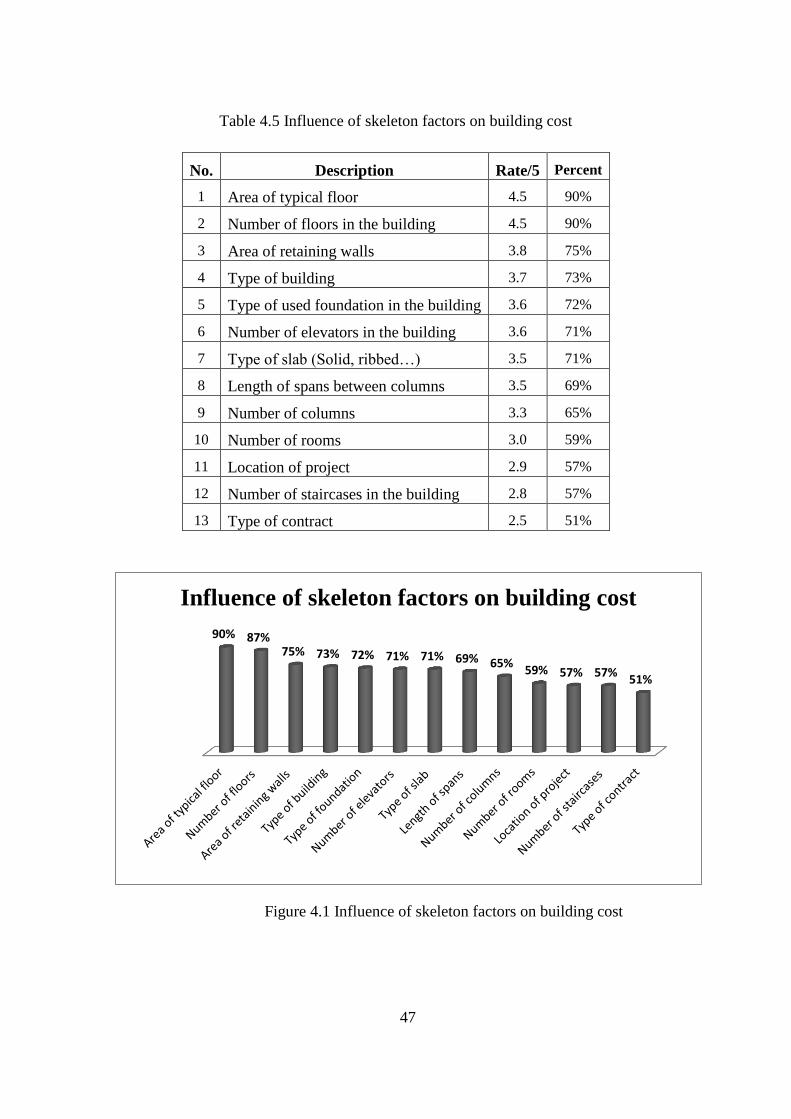
47

Table ‎4.5 Influence of skeleton factors on building cost

Figure ‎4.1 Influence of skeleton factors on building cost

90% 87% 75% 73% 72% 71% 71% 69% 65%

59% 57% 57% 51%

Influence of skeleton factors on building cost

No. Description Rate/5 Percent

1 Area of typical floor 4.5 90%

2 Number of floors in the building 4.5 90%

3 Area of retaining walls 3.8 75%

4 Type of building 3.7 73%

5 Type of used foundation in the building 3.6 72%

6 Number of elevators in the building 3.6 71%

7 Type of slab (Solid, ribbed…) 3.5 71%

8 Length of spans between columns 3.5 69%

9 Number of columns 3.3 65%

10 Number of rooms 3.0 59%

11 Location of project 2.9 57%

12 Number of staircases in the building 2.8 57%

13 Type of contract 2.5 51%

48

III. Finishing phase cost factors

Figure ‎4.2 shows the respondents views for the influence of 18 finishing parameters on

total building cost. It is found that the external finishing type has the highest rate (78%),

while volume of air-conditioning, area of curtain walls, type of tiling, type of sanitary,

and type of electrical works have a rate between 27%-76%.

These results reveal how convergence exists between most of parameters, and there is

no dominant parameter existing among them. However, as illustrated in Table ‎4.5 about

the indication of this convergence, but all of these parameters was subjected to evaluate

by relevant experts who presented their views and suggestion in next section.

49

Figure ‎4.2 Influence of finishing factors on building cost

78%

76%

74%

73%

73%

72%

69%

69%

68%

68%

67%

67%

65%

65%

64%

63%

62%

52%

Type of external plastering (78%)

Volume of Air-conditioning (76%)

Area of curtain walls (74%)

Type of tiling (73%)

Type of water and sanitary works (73%)

Type of electrical works (72%)

Area of gypsum board and false ceiling (69%)

Area of marble works (69%)

Firefighting and alarm works (68%)

Quantity of electrical works (68%)

Number of windows (67%)

Quantity of water and sanitary works (65%)

Type of carpentry works (65%)

Number of internal doors (65%)

Type of Aluminum works (64%)

Quantitiy of carpentry works (63%)

Quantity of metal works for protection anddecoration (62%)

Type of painting (52%)

Influence of finishing factors on building cost

50

4.1.2 Delphi Technique

Different technique has been used to determine the effective factors on building

project cost. This technique relies on the concept of Delphi technique, which aimed

to achieve a convergence of opinion on factors affecting the cost of the project. It

provides feedback to experts in the form of distributions of their opinions and

reasons. Then, they are asked to revise their opinions in light of the information

contained in the feedback. This sequence of questionnaire and revision is repeated

until no further significant opinion changes are expected (Creedy, et al., 2006).

For Delphi process, several rounds should be conducted where first round begins

with an open-ended questionnaire. The open-ended questionnaire serves as the

cornerstone of soliciting specific information about a content area from the Delphi

subjects, then after receiving the responses, the researcher converts the collected

information into a well-structured questionnaire to be used as the survey instrument

for the second round of data collection. In the second round, each Delphi participant

receives a second questionnaire and is asked to review the items summarized by the

investigators based on the information provided in the first round, where in this

round areas of disagreement and agreement are identified. However, in third round

Delphi panelist are asked to revise his/her judgments or to specify the reasons for

remaining outside the consensus. In the fourth and often final round, the list of

remaining items, their ratings, minority opinions, and items achieving consensus are

distributed to the panelists. This round provides a final opportunity for participants to

revise their judgments. Accordingly, the number of Delphi iterations depends largely

on the degree of consensus sought by the investigators and can vary from three to

five (Hsu, 2007).

Five experts in construction field were selected to reach a consensus about specifying

the key cost parameters The results with those five experts were significantly close to

the questionnaire results, and only three rounds were conducted due to largely degree

of consensus. where they proposed to exclude retaining wall and curtain wall from

these factors because of their rarity in Gaza‟s projects, In addition, for the two

factors; type of slab and length of span, they recommended to combine them with

one factor that contains slab with drop beams. Moreover, they suggested merging

area of gypsum board with HVAC (Heating Ventilation and Air-conditioning) to

51

avoid existing dependent parameters in input factors because gypsum boards are

installing in case of installing central air-conditioning.

4.1.3 Literature Studies

There are several key parameters that effect on buildings cost. Selecting the most

influential parameters is one of the superior challenge of building the model.

Therefore, many researchers studied these parameters and implemented their models

according to various parameters. After studying most of these parameters, part of

these were included in questionnaire survey while others were excluded due to

several reasons based on experts in this field, such as:

- Little impact on Gaza's building projects as temporary facilities.. etc.

- Rare use of these factors in Gaza's projects as vinyl exterior finish, Landscaping,

Usage of basement, parking area ..etc.

- Convergence of factors like area of gorund floor and area of typical floor, The

ratio of the typical floor area to the total area of the building, …etc.

- Assumptions and limitations that have been used in this study as year of project,

duration of implementing the project, ..etc.

Table ‎4.6 presents the influential factors that endorsed in former empirical models

and compatible with the adopted factors in this research.

Table ‎4.6 Influential factors adopted in previous researches

No. Chosen Factors References

1 Floor Area

(Kim, et al., 2004)

(Gunaydın & Dogan, 2004)

(Arafa & Alqedra, 2011)

(Cheng, et al., 2010)

(Sonmez, 2011)

(Wang, et al., 2012)

2 Number of storeys

(Kim, et al., 2004)




(Sonmez, 2011)

52

4.1.4 Influential Factors Adopted in the Research

Literature studies was the first process in determining the key parameters, then the

questionnaire that was designed according to these literatures as long as specialists

opinions, and finally Delphi technique that acquired a final identification of most

influential factors on building projects cost.

According to previous techniques, it is obvious that there is a substantial

convergence in identifying factors affecting on cost of building projects in Gaza

Strip. Therefore, it can be simply adopted the most influential factors (skeleton and

finishing factors). Table ‎4.7 shows the most influential factors that were adopted in

this study and were used in building the models as input parameters. It contains five

skeleton factors and six finishing factors.

No. Chosen Factors References

3 Slab type (Kim, et al., 2004)

(Doğan, 2005)

4 Finishing grades (Kim, et al., 2004)

5 Foundation type

(Kim, et al., 2004)




6 Number of elevator



(Sonmez, 2011)

7 Type of project (ElSawy, et al., 2011)

8 Type of contract (ElSawy, et al., 2011)

9 External finishing (Wang, et al., 2012)

(Sonmez, 2011)

53

Table ‎4.7 Influential Factors of building project Cost adopted in this research

No. Description Range

1 Area of typical floors Less than 1200 m2

2 Number of storeys (1-8) storey

3 Use of building

Prayer place-Resedential-Extension of

schools-Schools-Public buildings-Mosques

4 Type of foundation None-Isolated-Strap-Piles-Mat

5 Type of slab Solid- Ribbed - Drop beams

6 Number of elevators (0-1-2)

7 Type of external finishing None-Normal plaster- Marmarina- Natural

stone

8 Presence of HVAC and false ceiling None -Central conditioning-Split units

9 Type of tilling Ceramic –Terrazzo -Porcelain

10 Type of electricity works Basic - Luxury

11 Type of mechanical works Basic -Luxury

Data Collection 4.2

In fact, the process of collecting information that is related to cost estimation

problems is a difficult task especially in Gaza Strip, because such information is the

property of each construction firm. Construction firms usually do not agree to share

their cost data with other competing construction firms. Moreover, most firms

believe that such information usually makes a difference in being more competitive

in the market. However, great effort and time were exposed to collect adequate

account of building projects to establish an accurate neural network model. The

methodology for collecting these data was based on personal contacts with

construction firms, institutions and government ministries across Gaza Strip.

Data Validation 4.3

Data validation is paramount before developing any predictive model, which allows

identifying uncommon cases, invalid cases, erroneous variables and incorrect data

values in the dataset. If the data is prepared properly, it will be able to develop a more

realistic parametric cost model and give better results.

54

In order to overcome any defect in collected data, some basic assumptions and criteria

were defined and performed, which are:

- The project has to be completely finished or has approval for the funding

(Arafa & Alqedra, 2011).

- Project implemtation period less than one year (Arafa & Alqedra, 2011).

- Implementation of the project was during the period 2009 – 2012.

- Unifying currency of projects prices.

- Incomplete data, missing one or more values.

- Duplicate data, two projects are the same in all related values.

- Misleading data.

- The maximum amount of projects in a single category should not be more than

95% (Islam, et al., 2009).

- the maximum amount of categories with count of one (1) should not be more

than 90% (Islam, et al., 2009).

As a result of this filtering and checks, 24 projects of 193 projects were

eliminated. Subsequently, 169 projects were used to build the model.

Data Results 4.4

In this section, a detailed analysis of data and results will be presented and

elaborated by using frequency analysis. The data used in this study was collected

from 193 bids submitted to their office in the past three years. A data sheet was

prepared and used to extract all useful information from each project. Table ‎4.8

presents the main sources of data and the number of projects that have been obtained

from these sources.

Table ‎4.8 Data resources

Data Resources No. of projects Percentage (%)

Engineering Consulting Companies 23 12%

Contractors 77 40%

Government Ministries 38 20%

55

Data Resources No. of projects Percentage (%)

UNRWA 6 3%

Engineering Institutions 49 25%

Total 193 100%

As shown from Table ‎4.8, most institutions concerned with construction engineering

in Gaza strip were visited. 23 projects were obtained from engineering consulting

companies, 77 projects were gathered from contractors, and also 38 projects were

collected from government ministries concerned with construction projects; as

Ministry of Public Works and Housing, Ministry of local government and Ministry

of education, while 6 projects were obtained from UNRWA office, and finally 49

projects were collected from various institutions.

Use of building

Use of building factor includes six subtypes as shown in Table ‎4.9, some subtypes

were excluded like hospitals, laboratories, and universities because there is no

sufficient number of these types were implemented during (2009-2012).

As shown in Table ‎4.9, all subtypes have a good distribution of projects, where

residential subtype (30.8%), and public building (20%) have the maximum rate,

while schools have (17.8%), mosques (15.4%), Prayer place (6.5%), and school

extension (9.5%),

Table ‎4.9 Use of building factor

Use of building No. of projects Percentage (%)

Prayer place 11 6.5 %

Residential 52 30.8 %

School extension 16 9.5 %

Schools 30 17.8 %

Public building 34 20 %

Mosques 26 15.4 %

Total 169 100 %

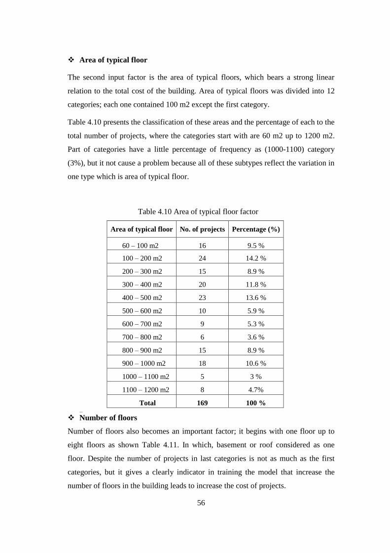
56

Area of typical floor

The second input factor is the area of typical floors, which bears a strong linear

relation to the total cost of the building. Area of typical floors was divided into 12

categories; each one contained 100 m2 except the first category.

Table ‎4.10 presents the classification of these areas and the percentage of each to the

total number of projects, where the categories start with are 60 m2 up to 1200 m2.

Part of categories have a little percentage of frequency as (1000-1100) category

(3%), but it not cause a problem because all of these subtypes reflect the variation in

one type which is area of typical floor.

Table ‎4.10 Area of typical floor factor

Area of typical floor No. of projects Percentage (%)

60 – 100 m2 16 9.5 %

100 – 200 m2 24 14.2 %

200 – 300 m2 15 8.9 %

300 – 400 m2 20 11.8 %

400 – 500 m2 23 13.6 %

500 – 600 m2 10 5.9 %

600 – 700 m2 9 5.3 %

700 – 800 m2 6 3.6 %

800 – 900 m2 15 8.9 %

900 – 1000 m2 18 10.6 %

1000 – 1100 m2 5 3 %

1100 – 1200 m2 8 4.7%

Total 169 100 % CDSFDFD S

Number of floors

Number of floors also becomes an important factor; it begins with one floor up to

eight floors as shown Table ‎4.11. In which, basement or roof considered as one

floor. Despite the number of projects in last categories is not as much as the first

categories, but it gives a clearly indicator in training the model that increase the

number of floors in the building leads to increase the cost of projects.

57

Table ‎4.11 Number of floors factor

Type of foundation

The most common foundation subtypes are isolated, strap, piles, and mat

respectively. Table ‎4.12 shows the number of projects in each subtype of foundation

and the percentage of each to the total number of projects. For the first subtype

“None”, it means there is existing foundation in the building but it need an extension

through building more floors. As presented, isolated foundation has the highest rate

(50.3%), and strap foundation has (25.4%), while piles and mat foundation have

(21.3%).

Table ‎4.12 Type of foundation factor

Type of foundation No. of projects Percentage (%)

None 5 3 %

Isolated 85 50.3 %

Strap 43 25.4 %

Piles 19 11.2 %

Mat 17 10.1 %

Total 169 100 %

Number of floors No. of projects Percentage (%)

1 30 17.8 %

2 39 23.1 %

3 66 39 %

4 16 9.5 %

5 6 3.6 %

6 2 1.2 %

7 3 1.8 %

8 7 4 %

Total 169 100 %

58

Type of slab

The type of slab affect on the total cost of project by the volume of concrete and the

amount of reinforcement. Table ‎4.13 presents three subtypes of slab solid slab (5.3

%), Ribbed slab (39.6 %), and slab with drop beams (55.1 %).

Table ‎4.13 Type of slab factor

Type of slab No. of projects Percentage (%)

Solid slab 9 5.3 %

Ribbed slab 67 39.6 %

Slab with Drop beams 93 55.1 %

Total 169 100 %

Number of elevators

The following Table ‎4.14 shows that over 89% of the data has no elevators in

buildings, 7.1% have one elevator and another 3% has two elevators in its structure

building.

Table ‎4.14 Number of elevator factor

Type of external finishing

Numerous subtypes of external finishing are using in Gaza Strip, Table ‎4.15

demonstrates these types and frequency for each, where Normal plaster has (44%),

and Marmarina (38.5%), while Natural stone (14%). For subtype “None” (4%) it

means the 4% of building haven‟t any type of external finishing.

Number of elevators No. of projects Percentage (%)

0 152 89.9 %

1 12 7.1 %

2 5 3 %

Total 169 100 %

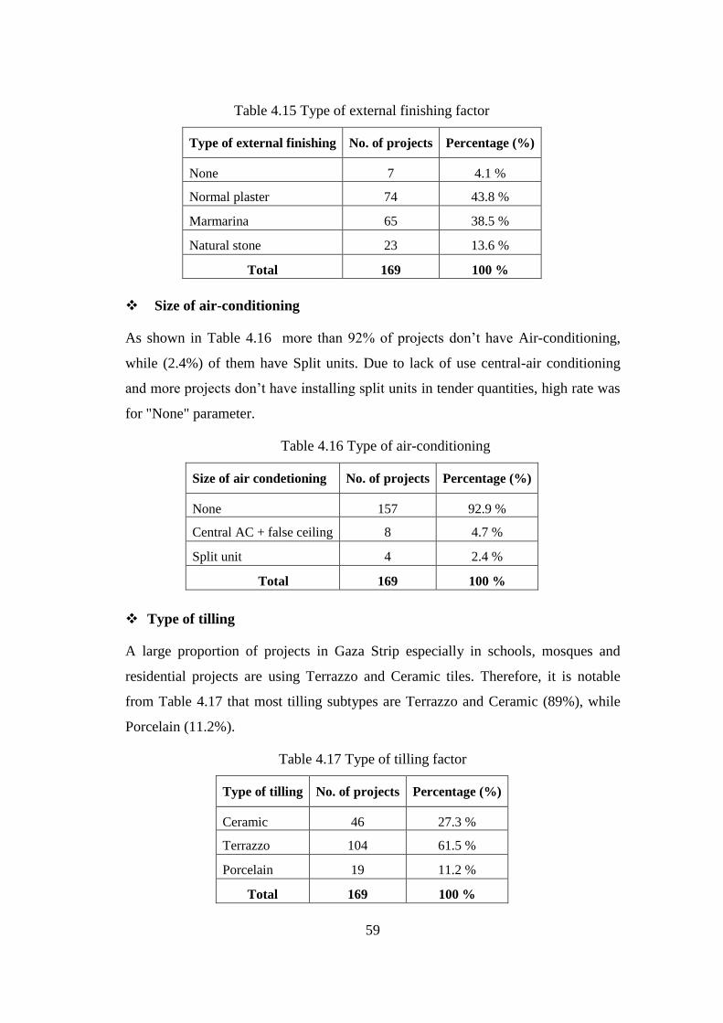
59

Table ‎4.15 Type of external finishing factor

Type of external finishing No. of projects Percentage (%)

None 7 4.1 %

Normal plaster 74 43.8 %

Marmarina 65 38.5 %

Natural stone 23 13.6 %

Total 169 100 %

Size of air-conditioning

As shown in Table ‎4.16 more than 92% of projects don‟t have Air-conditioning,

while (2.4%) of them have Split units. Due to lack of use central-air conditioning

and more projects don‟t have installing split units in tender quantities, high rate was

for "None" parameter.

Table ‎4.16 Type of air-conditioning

Size of air condetioning No. of projects Percentage (%)

None 157 92.9 %

Central AC + false ceiling 8 4.7 %

Split unit 4 2.4 %

Total 169 100 %

Type of tilling

A large proportion of projects in Gaza Strip especially in schools, mosques and

residential projects are using Terrazzo and Ceramic tiles. Therefore, it is notable

from Table ‎4.17 that most tilling subtypes are Terrazzo and Ceramic (89%), while

Porcelain (11.2%).

Table ‎4.17 Type of tilling factor

Type of tilling No. of projects Percentage (%)

Ceramic 46 27.3 %

Terrazzo 104 61.5 %

Porcelain 19 11.2 %

Total 169 100 %

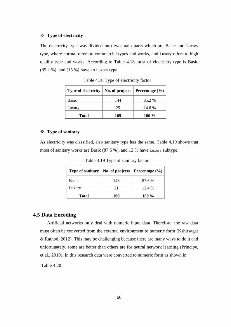
60

Type of electricity

The electricity type was divided into two main parts which are Basic and Luxury

type, where normal refers to commercial types and works, and Luxury refers to high

quality type and works. According to Table ‎4.18 most of electricity type is Basic

(85.2 %), and (15 %) have an Luxury type.

Table ‎4.18 Type of electricity factor

Type of electricity No. of projects Percentage (%)

Basic 144 85.2 %

Luxury 25 14.8 %

Total 169 100 %

Type of sanitary

As electricity was classified, also sanitary type has the same. Table ‎4.19 shows that

most of sanitary works are Basic (87.6 %), and 12 % have Luxury subtype.

Table ‎4.19 Type of sanitary factor

Type of sanitary No. of projects Percentage (%)

Basic 148 87.6 %

Luxury 21 12.4 %

Total 169 100 %

Data Encoding 4.5

Artificial networks only deal with numeric input data. Therefore, the raw data

must often be converted from the external environment to numeric form (Kshirsagar

& Rathod, 2012). This may be challenging because there are many ways to do it and

unfortunately, some are better than others are for neural network learning (Principe,

et al., 2010). In this research data were converted to numeric form as shown in

Table ‎4.20

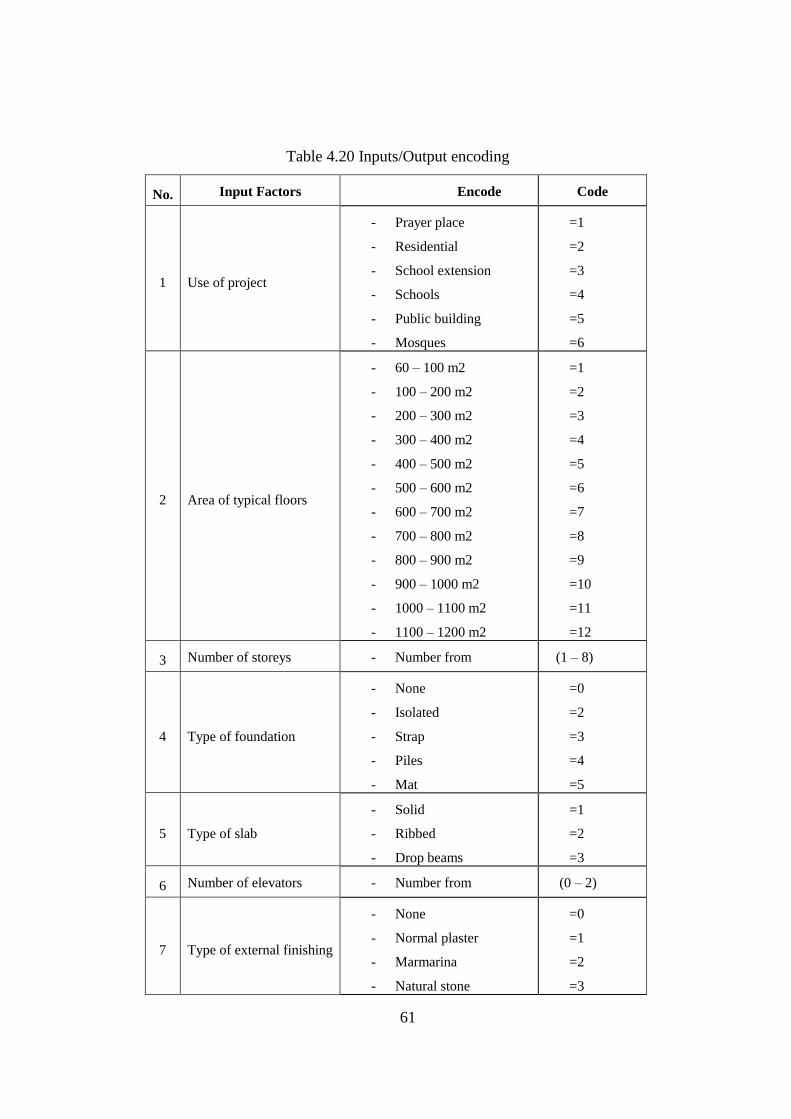
61

Table ‎4.20 Inputs/Output encoding

No. Input Factors Encode Code

1 Use of project

- Prayer place

- Residential

- School extension

- Schools

- Public building

- Mosques

=1

=2

=3

=4

=5

=6

2 Area of typical floors

- 60 – 100 m2

- 100 – 200 m2

- 200 – 300 m2

- 300 – 400 m2

- 400 – 500 m2

- 500 – 600 m2

- 600 – 700 m2

- 700 – 800 m2

- 800 – 900 m2

- 900 – 1000 m2

- 1000 – 1100 m2

- 1100 – 1200 m2

=1

=2

=3

=4

=5

=6

=7

=8

=9

=10

=11

=12

3 Number of storeys - Number from (1 – 8)

4 Type of foundation

- None

- Isolated

- Strap

- Piles

- Mat

=0

=2

=3

=4

=5

5 Type of slab

- Solid

- Ribbed

- Drop beams

=1

=2

=3

6 Number of elevators - Number from (0 – 2)

7 Type of external finishing

- None

- Normal plaster

- Marmarina

- Natural stone

=0

=1

=2

=3

62

No. Input Factors Encode Code

8 Size of air-conditioning

- None

- Central AC+False

ceiling

- Split unit

=0

=1

=2

9 Type of tilling

- Ceramic

- Basalt- Terrazzo

- Porcelain

=1

=2

=3

10 Type of electricity - Basic

- Luxury

=1

=2

11 Type of sanitary - Basic

- Luxury

=1

=2

No. Output Parameter Encode Code

1 Total Project cost - in dollars ($)

63

CHAPTER 5

5 Model Development

Introduction 5.1

A Neural Network training program, NeuroSolution, was used as a standalone

environment for Neural Networks development and training. Moreover, for

verifying this work, a plentiful trial and error process was performed to obtain the

best model architecture.

The following sections present the steps performed to design the artificial neural

network model, the limitation of adopted model, and finally the discussion and

analysis of results.

Model Limitations 5.2

In spite of great accuracy of using ANN in cost estimation, it has a considerable

defect, as it depends mainly on historical data; this dependency has several

disadvantages as the following;

- Diversity of variables for effective factors is limited to what available in

collected data.

- Data should contain sufficient projects for each variable.

- New variables which was not included in adopted model will not be handled.

Therefore, in this study most of construction variables used in Gaza Strip were

included except those that haven't enough frequency. After analyzing the collected

data, there was found that some limitations on input parameters should be assigned

to give the best output. Table ‎5.1 illustrates the available range of input data in ANN

model as; Area of typical floor has a range between 60 - 1200 m2, Number of floors

ranges from 1floor up to 8 floors, and Number of elevators also ranges from 0 to 2.

For remaining input factors as use of project, type of foundation... etc, they are also

limited to earlier mentioned choices. See section (‎4.1.4)

64

Table ‎5.1 Input limitations in model

Model Building 5.3

There are several types of ANNs softwares are used to predict the future values

based on the past data like SPSS, MATLAB, NeuroSolution …etc. Many

researchers used NeuroSolution application in building their neural networks that it

achieved good performance as (Edara, 2003; Gunaydın & Dogan, 2004; Bouabaz &

Hamami, 2008; Dowler, 2008; Attal, 2010; Wang, et al., 2012).

The developed model in this research based on NeuroSolution 5.07 for Excel

program. It was selected for its ease of use, speed of training, flexibility of building

and executing the NN model. In addition, the modeler has the flexibility to specify

his own neural network type, learning rate, momentum, activation functions,

number of hidden layers/neurons, and graphical interpretation of the results. Finally,

It has multiple criteria for training and testing the model.

1) Data Organization

Initially, the first step in implementing the neural network model in NeuroSolution

application is to organize the Neurosolution excel spreadsheet. Then, specifying the

input factors that have been already encoded, which consist of 11 factors; Type of

project, area of typical floor, number of floors, type of foundation, type of slab,

number of elevators, type of external finishing, type of air-conditioning, type of

tilling, type of electricity, and type of sanitary. The desired parameter (output)

which is (total cost of the project).

Models numeric variables Minimum value Maximum value

Floor Area 60 m2

1200 m2

Number of floors 1 storey 8 storey

Number of elevators 0 2

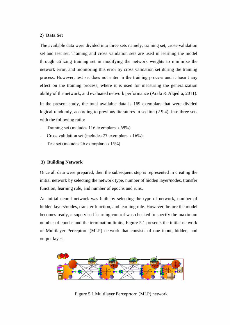
65

2) Data Set

The available data were divided into three sets namely; training set, cross-validation

set and test set. Training and cross validation sets are used in learning the model

through utilizing training set in modifying the network weights to minimize the

network error, and monitoring this error by cross validation set during the training

process. However, test set does not enter in the training process and it hasn‟t any

effect on the training process, where it is used for measuring the generalization

ability of the network, and evaluated network performance (Arafa & Alqedra, 2011).

In the present study, the total available data is 169 exemplars that were divided

logical randomly, according to previous literatures in section (2.9.4), into three sets

with the following ratio:

- Training set (includes 116 exemplars ≈ 69%).

- Cross validation set (includes 27 exemplars ≈ 16%).

- Test set (includes 26 exemplars ≈ 15%).

3) Building Network

Once all data were prepared, then the subsequent step is represented in creating the

initial network by selecting the network type, number of hidden layer/nodes, transfer

function, learning rule, and number of epochs and runs.

An initial neural network was built by selecting the type of network, number of

hidden layers/nodes, transfer function, and learning rule. However, before the model

becomes ready, a supervised learning control was checked to specify the maximum

number of epochs and the termination limits, Figure ‎5.1 presents the initial network

of Multilayer Perceptron (MLP) network that consists of one input, hidden, and

output layer.

Figure ‎5.1 Multilayer Perceprtorn (MLP) network

66

Before starting the training phase, the normalization of training data is recognized to

improve the performance of trained networks by Neurosolution program which as

shown in Figure ‎5.2 which ranging from (-1 to +1).

Model Training 5.4

The objective of training neural network is to get a network that performs best on

unseen data through training many networks on a training set and comparing the

errors of the networks on the validation set (Dindar, 2004). Therefore, several

network parameters such as number of hidden layers, number of hidden nodes,

transfer functions and learning rules were trained multiple times to produce the best

weights for the model.

As a preliminary step to filter the preferable neural network type, A test process was

applied for most of available networks in the application. Two types Multilayer

Perceptron (MLP) and General feed Forward (GFF) networks were chosen to be

focused in following training process due to their good initial results.

It is worthy to mention that, previous models that have been applied in the field of

cost estimation by neural networks used earlier two types of networks because of

giving them the best outcome.

Figure ‎5.2 Selecting the normalization limits of data

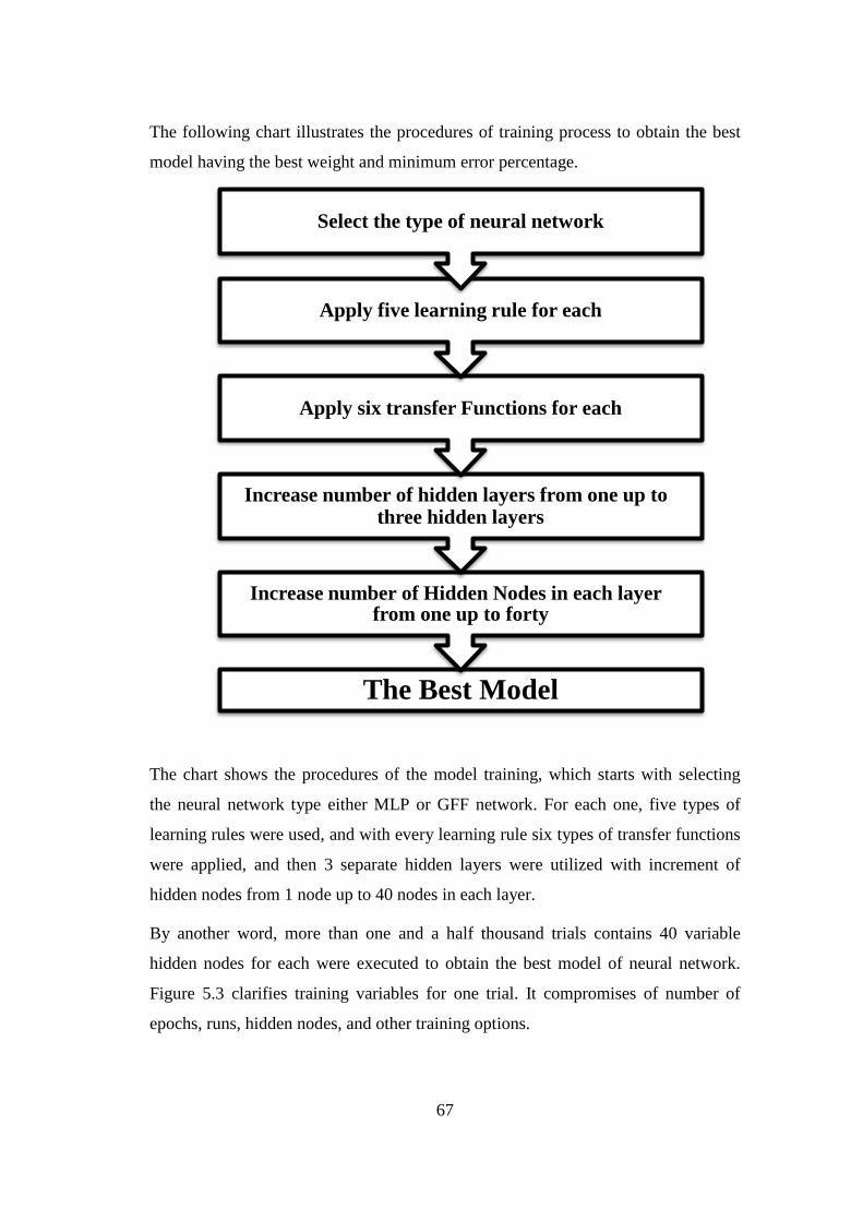
67

The Best Model

Increase number of Hidden Nodes in each layer from one up to forty

Increase number of hidden layers from one up to three hidden layers

Apply six transfer Functions for each

Apply five learning rule for each

Select the type of neural network

The following chart illustrates the procedures of training process to obtain the best

model having the best weight and minimum error percentage.

The chart shows the procedures of the model training, which starts with selecting

the neural network type either MLP or GFF network. For each one, five types of

learning rules were used, and with every learning rule six types of transfer functions

were applied, and then 3 separate hidden layers were utilized with increment of

hidden nodes from 1 node up to 40 nodes in each layer.

By another word, more than one and a half thousand trials contains 40 variable

hidden nodes for each were executed to obtain the best model of neural network.

Figure ‎5.3 clarifies training variables for one trial. It compromises of number of

epochs, runs, hidden nodes, and other training options.

68

Ten runs in each one 3000 epochs were applied, where a run is a complete

presentation of 3000 epochs, each epoch is a one complete presentation of all of the

data (Principe, et al., 2010). However, in each run, new weights were applied in the

first epoch and then the weights were adjusted to minimize the percentage of error in

other epochs.

To avoid overtraining for the network during the training process, an option of using

cross-validation was selected, which computes the error in a cross validation set at

the same time that the network is being trained with the training set.

The model was started with one hidden layer and one hidden node in order to begin

the model with simple architecture, and then the number of hidden PEs was growing

up by one node up to 40 hidden nodes.

Model Results 5.5

As mentioned above, the purpose of testing phase of ANN model is to ensure that

the developed model was successfully trained and generalization is adequately

achieved. Through a system of trial and error guided by earlier recommendation in

section (‎2.9.4), the best model that provided more accurate cost estimate without

Figure ‎5.3 Training options in Neurosolution application

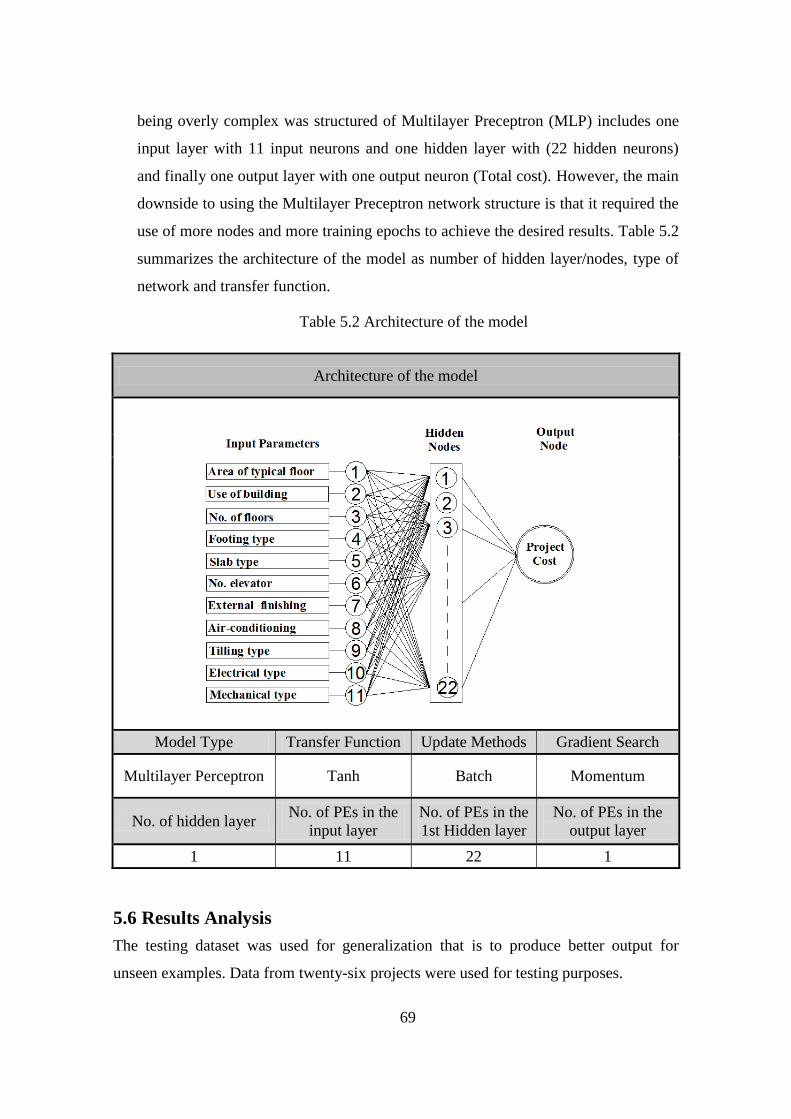
69

being overly complex was structured of Multilayer Preceptron (MLP) includes one

input layer with 11 input neurons and one hidden layer with (22 hidden neurons)

and finally one output layer with one output neuron (Total cost). However, the main

downside to using the Multilayer Preceptron network structure is that it required the

use of more nodes and more training epochs to achieve the desired results. Table ‎5.2

summarizes the architecture of the model as number of hidden layer/nodes, type of

network and transfer function.

Table ‎5.2 Architecture of the model

Results Analysis 5.6

The testing dataset was used for generalization that is to produce better output for

unseen examples. Data from twenty-six projects were used for testing purposes.

Architecture of the model

Model Type Transfer Function Update Methods Gradient Search

Multilayer Perceptron Tanh Batch Momentum

No. of hidden layer No. of PEs in the

input layer

No. of PEs in the

1st Hidden layer

No. of PEs in the

output layer

1 11 22 1

70

A Neurosolution test tool was used for testing the adopted model accordingly to the

weights adopted. Table ‎5.3 presents the results of these twenty-six projects with

comparing the real cost of tested project with estimated cost from neural network

model, and an absolute error with both price and percentage are also presented.

Table ‎5.3 Results of neural network model at testing phase

No.

Actual Cost ($) Estimated Cost

($)

Absolute

Error AE

($)

Absolute

Percentage

Error (%)

Project 1 23,200 25,624 2,424 10%

Project 2 34,710 35,366 656 1.8%

Project 3 211,200 220,043 8,843 4%

Project 4 441,600 399,836 41,764 9%

Project 5 318,450 297,602 20,848 7%

Project 6 286,000 310,767 24,767 9%

Project 7 33,050 35,366 2,316 7%

Project 8 720,000 751,343 31,343 4%

Project 9 444,540 440,324 4,216 0.9%

Project 10 616,150 650,536 34,386 6%

Project 11 320,000 272,113 47,887 15%

Project 12 355,238 272,113 83,125 23%

Project 13 112,980 108,282 4,698 4%

Project 14 1,106,640 914,035 192,605 17%

Project 15 936,660 856,575 80,085 9%

Project 16 375,000 356,332 18,668 5%

Project 17 901,236 881,406 19,830 2%

Project 18 835,395 778,954 56,441 7%

Project 19 1,051,400 994,410 56,990 5%

Project 20 977,208 994,410 17,202 2%

Project 21 1,032,105 994,410 37,695 4%

Project 22 1,012,194 994,410 17,784 2%

Project 23 997,000 994,410 2,590 0.2%

Project 24 1,110,000 1,108,615 1,385 0.1%

Project 25 2,030,400 2,087,698 57,298 3%

Project 26 1,149,000 1,137,167 11,833 1%

71

Mean Absolute Error

The Mean Absolute error (MAE) for the presented results in Table ‎5.3 equals (33,757

$), it is largely acceptable for projects worth hundreds of thousands dollars. However, it

is not a significant indicator for the model performance because it proceeds in one

direction, where the mentioned error may be very simple if the total cost of the project

is large, and in turn; it may be a large margin of error in case the total cost of the project

is small.

Mean Absolute Percentage Error

The mean absolute percentage error of the model is calculated from the test cases as

shown in Table ‎5.3, which equals 6%, this result can be expressed in another form by

accuracy performance (AP) according to Wilmot and Mei, (2005) which is defined as

(100−MAPE) %.

AP= 100% - 6% = 94%

That means the accuracy of adopted model for building projects estimate in conceptual

phase is 94%. It is a good result especially when this estimate in conceptual phase

where no details or drawings are available.

Total Mean Absolute Percentage Error

As mentioned in section (‎2.5) the allowable percentage error in cost estimation at

conceptual phase equals ±50%. Moreover, by reviewing many researches that used

ANN in cost estimation, it is shown that no specific percent of allowable error for

model estimate is available. However, the acceptable accuracy performance for ANN

model is equal 10% according to (Bakhary, et al., 2004) and (Samphaongoen, 2010).

In this study and according to Equation 2.5, the Total MAPE = 10%, where this error

includes all datasets as training, cross validation , and test datasets.

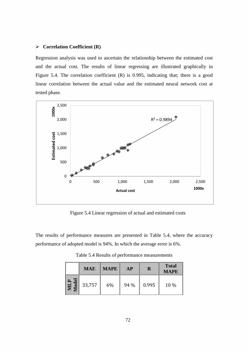
72

Correlation Coefficient (R)

Regression analysis was used to ascertain the relationship between the estimated cost

and the actual cost. The results of linear regressing are illustrated graphically in

Figure ‎5.4. The correlation coefficient (R) is 0.995, indicating that; there is a good

linear correlation between the actual value and the estimated neural network cost at

tested phase.

Figure ‎5.4 Linear regression of actual and estimated costs

The results of performance measures are presented in Table ‎5.4, where the accuracy

performance of adopted model is 94%. In which the average error is 6%.

Table ‎5.4 Results of performance measurements

R² = 0.9894

0

500

1,000

1,500

2,000

2,500

0 500 1,000 1,500 2,000 2,500

Esti

mat

ed c

ost

1

00

0x

Actual cost 1000x

MAE MAPE AP R

Total

MAPE

ML

P

Mod

el

33,757 6% 94 % 0.995 10 %

73

Figure ‎5.5 describes the actual cost comparing with estimated costs for cross validation

(C.V) dataset. It is noted that there is a slight difference between two cost lines.

For test dataset, A perfect agreement between the actual and estimated cost is shown in

Figure ‎5.6 which means the estimated values equal the actual ones.

Figure ‎5.5 Comparison between desired output and actual network output for C.V set

Figure ‎5.6 Comparison between desired output and actual network output for Test set

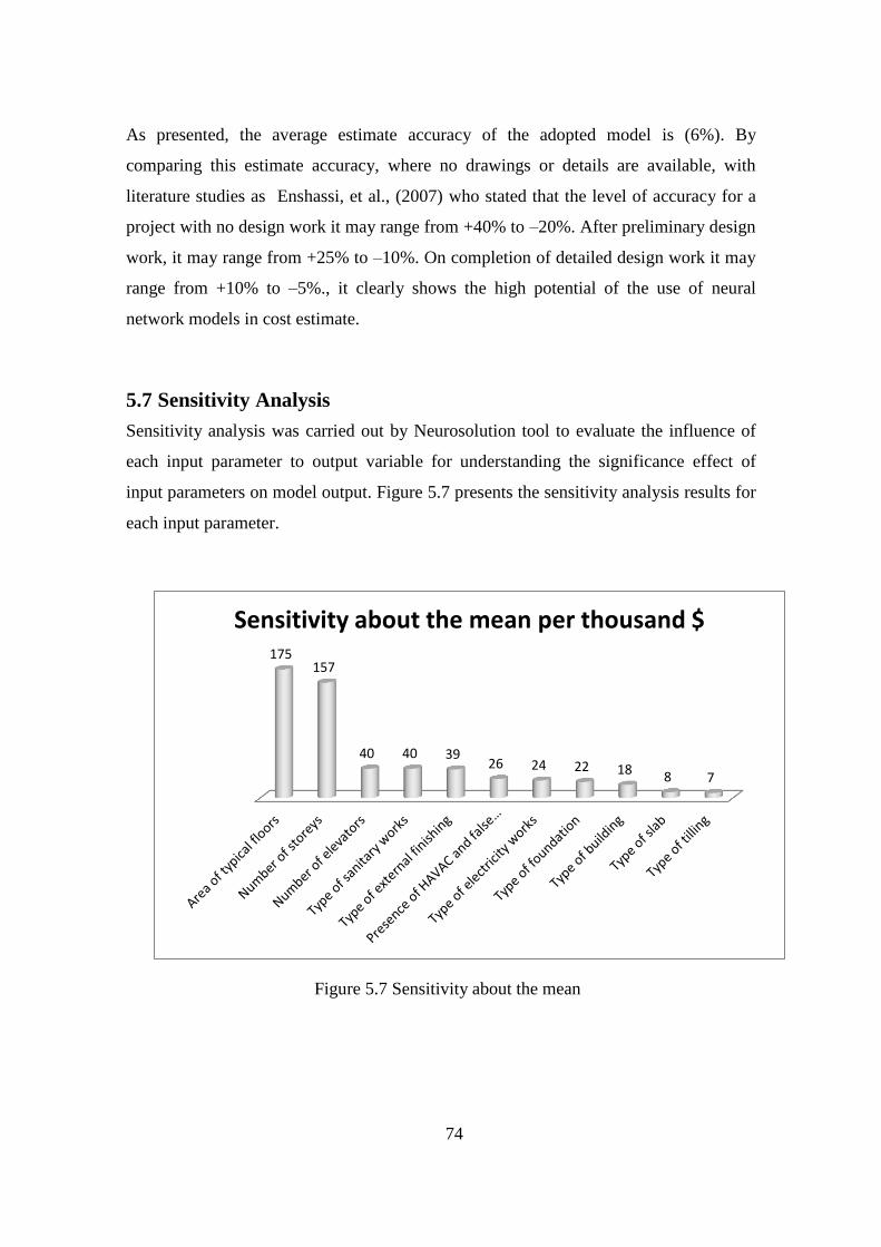
74

As presented, the average estimate accuracy of the adopted model is (6%). By

comparing this estimate accuracy, where no drawings or details are available, with

literature studies as Enshassi, et al., (2007) who stated that the level of accuracy for a

project with no design work it may range from +40% to –20%. After preliminary design

work, it may range from +25% to –10%. On completion of detailed design work it may

range from +10% to –5%., it clearly shows the high potential of the use of neural

network models in cost estimate.

Sensitivity Analysis 5.7

Sensitivity analysis was carried out by Neurosolution tool to evaluate the influence of

each input parameter to output variable for understanding the significance effect of

input parameters on model output. Figure ‎5.7 presents the sensitivity analysis results for

each input parameter.

Figure ‎5.7 Sensitivity about the mean

175 157

40 40 39 26 24 22 18 8 7

Sensitivity about the mean per thousand $

75

The increase of Standard Deviation refers to the strength influence of this parameter on

the overall cost of the project, Figure ‎5.7 shows that the Area of typical floor has the

highest rate of influence on the total cost of projects.

The value 175 for the area of typical floor input parameter is the value of the standard

deviation for 116 output values. These output values are recorded after training the

model with fixing the best weights on the mean value for each raw except the area of

typical floor value which is varied between (the mean – standard deviation) to (the mean

+ standard deviation).

Number of storeys has also a very significant influence, while the other parameters have

a considerable gab of influence on total cost than previous parameters. That means for

example; when changing type of foundation for a specific project and then changing the

area of typical floor for the same project, the comparison of influence of last parameter

on the output variable will be relatively great compared with effect of foundation type.

76

CHAPTER 6

6 Conclusion and Recommendations

Conclusion 6.1

This study aimed at developing a new technique for early cost estimate of building

projects in Gaza Strip, through developing a model that is able to help parties

involved in construction projects (owner, contractors, and others) in obtaining the total

cost information at the early stages of project with limited available information.

Several steps and procedures were conducted in order to achieve this aim as

following:

1- A questionnaire survey, expert interviews and exploratory search of previous

studies were used to identify the cost effective factors on building projects. Eleven

key parameters were adopted as most influential factors on building costs which are

use of building, area of typical floor, number of floors, type of foundation, type of

slab, number of elevators, type of air conditioning, external finishing, type of tile,

type of electricity, and type of sanitary.

2- Historical data of building projects were collected. The projects were executed

between 2009 and 2012 in Gaza Strip, from government ministries, UNRWA,

engineering institutions, contractors and consultants. The data was analyzed and

some of data were excluded due to some basic conditions. The final available

data were 169 projects which were divided randomly into three sets as training

set (116 projects), cross validation set (27 projects), and testing set (26 projects).

3- Developing ANN model passed through several steps started with selecting the

application to be used in building the model. The Neurosolution5.07 program

was selected for its efficiency in several previous researches in addition to its

ease of use and extract results. The data sets were encoded and entered into MS

excel spreadsheet to start training process for different models.

77

4- Many models were built but the best model that provided more accurate results

was Multilayer Perceptron network model (MLP) which structured from one

input layer included 11 input neurons, one hidden layer contained 22 hidden

neurons, one output neuron, tanh transfer function, and Moentum learning rate

which belongs to Backpropagation algorithm.

5- The accuracy performance of the adopted model recorded 94% where the model

performed well and no significant difference was discerned between the

estimated output and the actual budget value. The acceptable error rate in early

stage of building projects as mentioned in researches and studies is ranging

between (20-50%) while the average percentage error of this model is 6%.

6- In order to ensure the validity of the model in estimating the cost of new

projects, many statistical performance measures were conducted i.e; Mean

Absolute Error (MAE), Mean Absolute Percentage Error (MAPE), Total Mean

Absolute Percentage Error (Total MAPE), and Correlation Coefficient (r). The

results of these performance measures were acceptable and reliable, where the

mean percentage error of the model was 6%, and the total mean absolute

percentage error was 10%.

7- Sensitivity analysis was performed using Neurosolution tool to study the

influence of adopted factors on building costs, the concept of calculating

sensitivity analysis of input factors based on determining the standard deviation

of each. However, the performed sensitivity analysis was in general logically

where the area of typical floor and number of floors had the highest influence,

then number of elevators, sanitary type, number of elevators, electricity type,

type of external finishing, type of electricity, type of foundation, type of

building, type of slab, and type of tilling respectively had less effect

respectively.

8- The approach as presented is capable of providing accurate estimates of project

cost by using eleven parameters at the early design phase.

9- Some assumption and limitation were assumed in the study according to

available collected data. These limitations include the available choices of each

factor as Area of typical floors for example, has limited area between 60 m2 to

1000 m2, as well as the other input factors.

78

Recommendations 6.2

The current study showed very promising results in predicting the cost of building

projects, and this approach will continue to make impressive gains especially in civil

engineering field. However, some recommendations should be presented for decision-

makers in the construction sector and future studies to support the findings of this study;

1. All construction parties are encourged to be more aware about cost estimation

development and pay more attention for using this developed technique in

estimation process.

2. Government and engineering assosiations are recommended to establich a database

for executed projects for researchers to develop cost estimation process.

3. For future studies, it is recommended to obtain more training data from newly

projects and add them to the training data. This will improve the training process

and produce more input choices.

4. Finally, Cost estimates in neural network models are related to the input costs that

the model was built upon, so changing time or cost will increase the estimate error

or make the model unusable. Therefore, It is recommend to link the model with

price changes through cost index technique.

79

CHAPTER 7

7 References

AACE International Recommended Practice, 2010. Cost Engineering Terminology,

TCM Framework: No. 10S-90, pg 24.

AACE International, 2007. Cost engineering terminology, recommended practice.

[Online] Available at: www.aacei.org [Accessed 5 May 2012].

AACE Recommended Practice and standard, 1990. Standard cost engineering

terminology., s.l.: AACE, Inc. No.10s-90, .

Abdal-Hadi, M., 2010. Factors Affecting Accuracy of Pre-tender Cost Estimate in

Gaza Strip., Gaza strip. Master thesis in construction management, The Islamic

University of Gaza Strip.

Adeli, H. & Wu, M. Y., 1998. Regularization neural network for construction cost

estimation. Journal of Construction Engineering and Management-Asce, 124(1), pp. 18-

24.

Akintoye, A. & Fitzgerald, E., 1999. A survey of current cost estimating practices in

the UK,. Construction Management and Economics, 18(1), pp. 161-172.

Al-Najjar, H., 2005. Prediction of Ultimate Shear Strength of Reinforced Concrete

Deep Beams Using Artificial Neural Networks, Gaza strip. Master thesis in construction

management, The Islamic University of Gaza Strip..

Al-Shanti, Y., 2003. A Cost Estimate System for Gaza Strip Construction

Contractors, Palestine, Master thesis in construction management, The Islamic

University of Gaza Strip.

Al-Thunaian, S., 1996. Cost estimation practices for buildings by A/E firms in the

eastern province, Saudi Arabia. Unpublished master thesis in construction engineering

and management, Dhahran, Saudi Arabia. Master thesis in construction engineering and

management. King Fahd University of Petroleum and Minerals.

80

Aneja, N., 2011. Neural networks approach v/s Algorithmic approach : A study

through pattern recognition. An International Journal ( ACIJ ), 2(6).

Arafa, M. & Alqedra, M., 2011. Early stage cost estimation of buildings

construction projects using ANN. Journal Of Artifical Intelligence, 4(1), pp. 63-75.

Attal, A., 2010. Development of Neural Network Models for Prediction of Highway

Construction Cost and Project Duration, USA: Ohio University.

Ayed, A. S., 1997. Parametric Cost Estimating of Highway Projects using Neural

Networks, Canada: National Library of Canada.

Bakhary, N., Yahya, K. & Nam, N. C., 2004. Univariate Artificial Neural Network

In Forecasting Demand Of Low Cost House In Petaling Jaya. Jurnal Teknologi, 40(B),

June, pp. 67-75.

Bode, J., 1998. Decision support with neural networks in the management of

research and development: Concepts and application to cost estimation. Information &

Management, Volume 34, pp. 33-40.

Bouabaz, M. & Hamami, M., 2008. A Cost Estimation Model for Repair Bridges

Based on Artificial Neural Network. American Journal of Applied Sciences, 5(4), pp.

334-339.

Caputo, A. & Pelagagge, P., 2008. Parametric and neural methods for cost

estimation of process vessels. Int. J. Production Economics, Volume 112, p. 934–954.

Cavalieri, S., Maccarrone, P. & Pinto, R., 2004. Parametric vs. neural

networkmodels for the estimation of production costs: A case study in the automotive

industry. Int. J. Production Economics , Volume 91, p. 165–177.

Cengiz, Y., Gunes, F. & Caglar, M., 2005. Soft computing methods in microwave

active device modeling. Turkish Journal of Electrical Engineering and computer

science, 13(1).

Cheng, M.-Y., Tsai, H.-C. & Sudjono, E., 2010. Conceptual cost estimates using

evolutionary fuzzy hybrid neural network for projects in construction industry. Expert

Systems with Applications 37, p. 4224–4231.

81

Choon, T. & Ali, K. N., 2008. A review of potential areas of construction cost

estimating and identification of research gaps. Journal Alam Bina, 11(2), pp. 61-72.

Christian, D., Robert, W., Colin, H. & Martin, B., 2000. Modelling Ranunculus

Presence in the Rivers Test and Itchen Using Artificial Neural Networks. [Online]

Available at: http://www.geocomputation.org/2000/GC016/Gc016.htm

[Accessed 2 3 2013].

CII, Construction industry institute, 1998. Improving early estimates. Austin, USA:

university of Texas.

Clough, R., 1986. Construction Controlling. 5th ed. New York: John Wiley & Sons.

Creedy, G. D., Skitmore, M. & Sidwell, T., 2006. Risk factors leading to cost

overrun in the delivery of highway construction projects, Australia: Research Centre:

School of Urban Development.

Dindar, Z., 2004. Artificial Neural Networks Applied To Option Pricing., s.l.: s.n.

Doğan, S., 2005. Using machine learning techniques for early cost estimation of

structural systems of buildings, İZMİR: İzmir Institute of Technologyin.

Dowler, J., 2008. Using Neural Networks with Limited Data to Estimate

Manufacturing Cost, Master thesis in science. Ohio University.

Duran, O., Rodriguez, N. & Consalter, L., 2009. Neural networks for cost estimation

of shell and tube heat exchangers. Expert Systems with Applications, Volume 36, p.

7435–7440.

Dysert, L. R., 2006. Is "estimate accuracy" an oxymoron?, AACE International

Transactions, s.l.: EST01.1 - 01.5.

Edara, P., 2003. Mode Choice Modeling Using Artificial Neural Networks, Virginia.

Master thesis in civil engineering. Virginia Polytechnic Institute and State university.

Elhag, S., Boussabaine, H. & Ballal, A., 2005. Critical determinants of construction

tendering costs: quantity surveyors_ standpoint. International Journal of Project

Management, 23(7), p. 538–545.

82

ElSawy, I., Hosny, H. & Abdel Razek, M., 2011. A Neural Network Model for

Construction Projects Site Overhead Cost Estimating in Egypt. International Journal of

Computer Science Issues (IJCSI), 8(1).

Enshassi, A., Mohamed, S. & Madi, I., 2007. Cost estimation practice in the Gaza

Strip: A case study. The Islamic University Journal, 15(2), pp. 153-176.

Feng, W., Zhu, W. & Zhou, Y., 2010. The Application of Genetic Algorithm and

Neural Network in Construction Cost Estimate. Guangzhou, P. R. China, 29-31,July

2010, pp.. Guangzhou, China, s.n., pp. 151-155.

Gunaydın, M. & Dogan, Z., 2004. A neural network approach for early cost

estimation of structural systems of buildings. International Journal of Project

Management, Volume 22, p. 595–602.

Harding, A. et al., 1999. Implementation of a neural network model for the

comparison of the cost of different procurement approaches. In: Hughe. s.l., Liverpool

John Moores University, pp. 763-772.

Haykin, S., 1999. Neural Networks A comprehensive Fundamentals 2nd ed.. New

Jersey: Prentice-Hall.

Hegazy, T. & Ayed, A., 1998. Neural Network Model For Parametric Cost

Estimation Of Highway Projects. Journal Of Construction Engineering And

Management, pp. 210-218.

Hegazy, T., Moselhi & O., P. F. &., 1994. Developing Practical Neural Network

Applications Using Back- Propagation. Microcompurers in Civil Engineering, Volume

9, pp. 145- 159.

Hegazy, T. & Moselhi, O., 1995. Elements of Cost Estimation: A Survey in Canada

and the United States. Cost Engineering, 37(5), pp. 27-31.

Hinze, J., 1999. Construction Planning and Scheduling. Columbus, Ohio.: Prentice

Hall.

Hsu, C., 2007. The Delphi Technique:Making Sense Of Consensus. Practical

Assessment, Research & Evaluation electronic journal, 12(10).

Humphreys, K., 2004. Project and cost engineers. 4th ed. s.l.:Marcel Dekker.

83

Islam, S., Zhou, L. & Li, F., 2009. Application of Artificial Intelligence (Artificial

Neural Network) to Assess Credit Risk: A Predictive Model For Credit Card Scoring,

Karlskrona, Sweden: Blekinge Institute of Technology.

Jitendra, Vikas, Kuldeep & Samiksha, 2011. Cost prediction using neural network

learning techniques. IJCSMS International Journal of Computer Science and

Management Studies, 11(2).

Karna, K. N. & Breen, D. M., 1989. An artificial neural networks tutorial. The

international journal of neural networks, 1(1), pp. 4-23.

Kim, G.-H., An, S.-H. & Kang, K.-I., 2004. Comparison of construction cost

estimating models based on regression analysis, neural networks, and case-based

reasoning. Building and Environment, February, Volume 39, p. 1235 – 1242.

Kriesel, D., 2005. A Brief Introduction to Neural Networks. Germany: ..

s.l.:www.dkriesel.com.

Kshirsagar, P. & Rathod, N., 2012. Artificial Neural Network. International Journal

of Computer Applications.

Leng, K. C., 2005. Principles of knowledge transfer in cost estimating conceptual

model, Malaysia: University Teknologi Malaysia.

Liu, L. & Zhu, K., 2007. Improving cost estimates of construction projects using

phased cost factors. Journal of Construction Engineering and Management, 133(1), pp.

91-95.

Mahamid, I. & Bruland, A., 2010. Preliminary Cost Estimating models for Road

Construction Activities. [Online] Available at:

ttp://www.fig.net/pub/fig2010/papers/fs04e%5Cfs04e_mahamid_bruland_4592.pdf

[Accessed 1 2013].

Marjuki, M., 2006. Computerized building cost estimating system, Malaysia:

University Teknologi Malaysia.

McCaffer, R. & Baldwin, A. N., 1991. Estimating and Tendering for Civil

Engineering Works. 2nd ed. Oxford: BSP Professional Books.

84

Mohaghegh, S., 2000. Virtual Intelligence And Its Applications In Petroleum

Engineering. [Online] Available at: http://www.pe.wvu.edu/research/part1.htm

[Accessed 17 2 2013].

Naoum, S. G., 2007. Dissertation Research and Writing for Construction Students.

2nd Edition ed. London: Elsevier Ltd.

Nygren, K., 2004. Stock Prediction – A Neural Network Approach., s.l.: Royal

Institute of Technology.

Ostwald, P., 2001. Construction cost analysis and estimating.. s.l.:Upper Saddle

River., N.J. : Prentice Hall.

Pawar, R., 2007. Predicting Bid Prices In Construction Projects Using Non-

Parametric Statistical Models. USA: Texas A&M University.

Popescu, C., Phaobunjong, K. & Ovararin, N., 2003. Estimating Building Costs.

New York: Marcel Dekker, Inc.

Principe, J. et al., 2010. NeuroSolution Help, s.l.: NeuroDimension, Inc.

Rezaian, A., 2011. Time-Cost-Quality-Risk of Construction and Development

Projects or Investment. Middle-East Journal of Scientific Research, 10(2), pp. 218-223.

Samphaongoen, P., 2010. A Visual Approach to Construction Cost Estimating,

Milwaukee, Wisconsin : Marquette University.

Smith, A. E. & Mason, A. K., 1997. Cost estimation predictive modeling:

Regression versus neural network. The Engineering Economist, Volume 42(2), p. 137–

161.

Sodikov, J., 2005. Cost estimation of highway projects in developing countries:

artificial neural network approach. the Eastern Asia Society for Transportation Studies,

Volume 6, pp. 1036 - 1047.

Sonmez, R., 2004. Conceptual cost estimation of building projects with regression

analysis and neural networks. Canadian Journal of Civil Engineering, 31(4), pp. 677-

683.

85

Sonmez, R., 2011. Range estimation of construction costs using neural networks

with bootstrap prediction intervals. Expert Systems with Applications, Issue 38, p. 9913–

9917.

Stewart, R. D., 1991. Cost Estimating. 2nd ed. New York: John Wiley & Sons, Inc.

Swingler, K., 1996. Applying neural networks, A practical guide. 3rd edition ed.

s.l.:Morgan Kaufmann.

Verlinden, B., Duflou, R., Collin, D. & Cattrysse, D., 2007. Cost estimation for

sheet metal parts using multiple regression and artificial neural networks: A case study..

Journal of Construction Engineering and Management (ASCE), Volume 127(2), p. 93–

100.

Wang, Q., 2007. Artificial neural networks as cost engineering methods in a

collaborative manufacturing environment. Int. J. Production Economics, Volume 109,

p. 53–64.

Wang, W., Wang, S., Tsui, Y. & Hsu, C., 2012. A factor-based probabilistic cost

model to support bid-price estimation. Expert Systems with Applications, Volume 39, p.

5358–5366.

Wang, Y., Yu, C. & Chan, H., 2012. Predicting construction cost and schedule

success using artificial neural networks ensemble and support vector machines

classification models. International Journal of Project Management, Volume 30, p.

470–478.

Weckman, G. et al., 2010. Using neural networks with limited data to estimate

manufacturing cost. Journal of Industrial and Systems Engineering, 3(4), pp. 257-274.

Westney, R. E., 1997. The engineer’s Cost Handbook Tools for managing Project

Cost. s.l.:Marcel Dekker, Inc..

Willmott, C. & Matsuura, K., 2005. Advantages of the mean absolute error (MAE)

over the root mean square error (RMSE) in assessing average model performance.

Climate Research, Volume 30, p. 79–82.

86

8 Annex 1: Questionnaire

The questionnaire (In Arabic & English)

87

اصخببت حىل

غزة قطبع في انببي إشبء يشبريع في انخضعير عهيت عهى انؤثرة انعىايم

Influential factors on prices of building projects in

Gaza Strip

األخ انهذس/ األخج انهذصت ... ححيت طيبت وبعذ,

االجابة عمى ان لمساهمتكم في رفعاالو الشكر بجزيل لسيادتكم نتقدم فإننا , غزة قطاع في اإلنشاءات قطاع ألهمية رانظهذه االستبانة التي تهدف الى دراسة العوامل المؤثرة عمى تسعير مشاريع انشاء المباني في قطاع غزة, وذلك من خالل

التركيز عمى اهم العوامل الحرجة التي تؤثر عمى التسعير, كما نود ان نؤكد لسيادتكم عمى النقاط التالية: ي مشاريع انشاء المباني في قطاع غزة من خالل دراسة العوامل يركز هذا البحث عمى تسعير العطاءات ف -1

الداخمية لممباني والتي تؤثر بشكل قوي عمى عممية التسعير وعمى السعر االجمالي لتكمفة المشروع.جميع المعمومات التي يتم الحصول عميها منكم سوف تستخدم لغرض البحث العممي بهدف التطوير وسيتم -2

عمى سرية المعمومات الخاصة بكم. االلتزام بالمحافظة

يكىبث االصخبيب :

التعريف بالجهة المعنية. الجزء االول:

- : قمسين العوامل التي تؤثر عمى عممية التسعير في مشاريع انشاء المباني في قطاع غزة ويتكون من الجزء الثاني:\ )البناء الهيكمي(.العوامل المتعمقة بعممية االنشاء االساسية لممباني

العوامل المتعمقة بعممية تشطيب المبنى. -

لمباحث الهندسية، المشاريع إدارة في الماجستير درجة لنيل التكميمي البحث من جزء هي الدراسة هذه بأنما عم

نبيل الصوالحي / لدكتورا إشراف تحت, عمر محمد شحتو /المهندس

وإي أث جهذكى وإجبببحكى عهى األصئهت انطروحت في االصخبيب

وحقبهىا فبئق االحخراو وانخقذير

/ م. عمر محمد شحتو الباحث

2012طثرثز/

غزة –انجبيعت اإلصالييت

عبدة انذراصبث انعهيب

إدارة انخشييذ –كهيت انهذصت

The Islamic University –Gaza

Higher Education Deanship

Faculty of Engineering

Construction Management

88

أوال: انخعريف ببنجهت انعيت

انجهت انخي حقىو بخعبئت االصخببت

اىل )وسارج, تيذح, ؤطظح اهيح حيح او دوىح( __ نرة اطرشار __ شزمح قاوالخ __

انىقع انىظيفي ن يقىو بخعبئت االصخببت

...................... أخزي__ هذص ىقغ __ذز شزوع __ صاحة شزمح__

ن يقىو بخعبئت االصخببت في يجبل االشبءاث عذد صىاث انخبرة

طىاخ 10 أمثز __ طىاخ __10-7 طىاخ 6-4 __ طىاخ 1-3 __

عذد انشبريع انخعهقت ببشبء انببي انجزة خالل انضىاث انخش األخيرة ن يقىو بخعبئت االصخببت

شزوع 15 أمثز __ شزوع __11-15 شارغ 10-6__ شارغ 5-1__

( ذحذد ذي قىج ذأثز اىؼاو ػي ػيح اىرظؼز ف 5( إى )0االرقا ) شارغ إشاء اىثا

( شز اى ػذ ذاثز هذا اىؼاو هائا ػي ػيح اىرظؼز تا شز 0وجهح ظزك, حث ا اىزق )

( اى اىؼاو االمثز ذأثزا.5اىزق )

ف اىزتغ حظة قىج اىرأثز)×( اىزجاء وضغ اشارج

انجزء انثبي: انعىايم انؤثرة عهى عهيت انخضعير في يشبريع اشبء انببي في قطبع

غزة

89

Organization characteristics

__Contracting __Consultant __Owner (ministry, municipality,..)

Job title

__Company owner __ Project manager __Site engineer __Other

Experience years in construction industry

__1-3 years __4-6 years __ 710 years __more than 10 years

Number of building projects worked in during last five years

__1-5 projects __ 6-10 projects __ 11-15 projects __ more than 15 projects

- Numbers between (0-5) determine the weight of parameter on the total cost of

building cost.

- Number zero refers that this parameter does not has effect on the cost, while

number five refers that this parameter haa a huge influence on cost.

Second part: Factors affecting the pricing process in the construction

of buildings projects in the Gaza

90

أوال: انعىايم انخعهقت بعهيت االشبء االصبصيت نهبى )انببء انهيكهي(

(Factorالعامل المؤثر ) الرقم درجة تأثير العامل على عملية التسعير

0 1 2 3 4 5

1.1

Type of used foundation in the

building

اىقىاػذ اىظرخذح ف اىثىع

1.2 Area of typical floor

ىيث اىرنزر اىطاتق ظاحح

1.3 Number of floors in the building

.ػذد اىطىاتق ف اىث

1.4 Number of columns

ػذد االػذج ف اىث

1.5 Number of rooms

المبنى ف الغرف عدد

1.6 Number of elevators in the building

.اىصاػذ ف اىث ػذد

1.7 Type of slab (Solid, Ribbed …)

.صد, فزؽ, ..(( ىع اىظقف ىيث

1.8 Number of staircases in the building

ػذد االدراج ف اىث

1.9 Type of contract (Ls, unit)

.ىع اىؼقذ )قطىػح,وحذاخ حظىتح(

1.10 Length of spans between columns

اىظافاخ ت االػذج

1.11 Area of retaining walls in project

ظاحح اىجذرا االطرادح ىرفذ اىث

91

1.12 Location of project

ىقغ اشاء اىث

1.13 Use of building

اطرخذا اىث

انعىايم انخعهقت في عهيت حشطيب انبى ثبيب:

(Factorالعامل المؤثر ) الرقم درجة تأثير العامل على عملية التسعير

0 1 2 3 4 5

2.1 Type of external plastering

ىع اىنظىج اىخارجح

2.2 Type of painting

ىع اىذها

2.3 Type of tiling

ىع اىثالط

2.4 Area of marble works

مح اػاه اىزخا

2.5 Area of curtain walls

ظاحح اىىاجهاخ اىشجاجح

2.6 Number of internal doors

ػذد االتىاب اىذاخيح

2.7

Quantity of metal works for protection

and decoration

والدكور للحماة المستخدم الحدد كمة

2.8 Type of water and sanitary works

ىع االػاه اىصحح اىظرخذح

92

2.9 Quantity of water and sanitary works

مح االػاه اىصحح اىظرخذح

2.10 Firefighting and alarm works.

وجىد اػاه اذار واطفاء ىيحزق

2.11 Volume of HVAC works.

حج اػاه اىرنف

2.12 Quantity of electrical works

مح االػاه اىنهزتائح

2.13 Type of electrical works

ىع االػاه اىنهزتائح

2.14

Area of gypsum board and false

ceiling

ظاحح اػاه اىجثض واالطقف اىظرؼارج

2.95 Type of carpentry works

ىع اػاه اىجارج

2.96 Quantity of carpentry works

مح اػاه اىجارج

2.97 Number of windows

اىشثاتل ػذد

2.98 Type of Aluminum works

اىظرخذ االىى ىع

93

9 Annex 2 : Collected Projects

Collected projects

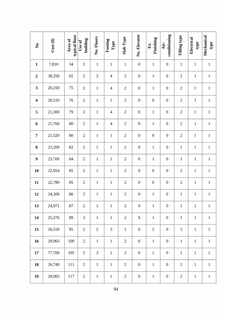
94

Mec

ha

nic

al

typ

e

Ele

ctri

cal

typ

e

Til

lin

g t

yp

e

Air

-

con

dit

ion

ing

Ex

.

Fin

ish

ing

No

. E

lev

ato

r

Sla

b T

yp

e

Fo

oti

ng

Ty

pe

No

. F

loo

rs

Use

of

bu

ild

ing

Are

a o

f

typ

ica

l fl

oo

r

Co

st (

$)

No

1 1 1 0 1 0 1 1 1 2 34 7,810 1

1 1 2 0 1 0 2 4 2 2 65 38,350 2

1 1 2 0 1 0 2 4 1 2 75 20,250 3

1 1 2 0 0 0 2 1 1 2 76 20,510 4

1 1 2 0 1 0 2 4 1 2 79 21,300 5

1 1 2 0 1 0 2 4 1 2 80 21,760 6

1 1 2 0 0 0 2 1 1 2 80 21,520 7

1 1 1 0 1 0 2 1 1 2 82 23,200 8

1 1 1 0 1 0 2 1 1 2 84 23,700 9

1 1 2 0 0 0 2 1 1 2 85 22,954 10

1 1 2 0 0 0 2 1 1 2 85 22,780 11

1 1 1 0 1 0 2 1 1 2 86 24,300 12

1 1 1 0 1 0 2 1 1 2 87 24,971 13

1 1 1 0 1 0 2 1 1 2 89 25,276 14

1 1 3 0 2 0 1 3 2 2 95 56,550 15

1 1 1 0 1 0 2 1 1 2 100 29,963 16

1 1 1 0 1 0 2 1 3 5 105 77,700 17

1 1 2 0 1 0 2 1 1 2 111 26,740 18

1 1 2 0 1 0 2 1 1 2 117 28,065 19

95

1 1 2 0 1 0 2 1 1 2 118 29,499 20

1 1 2 0 1 0 2 1 1 2 125 32,075 21

1 1 2 0 2 0 2 1 2 5 130 104,608 22

1 1 2 0 1 0 2 1 1 2 130 33,050 23

1 1 2 0 1 0 2 1 1 2 135 34,710 24

1 1 2 0 1 0 2 1 1 2 140 35,710 25

1 1 2 0 1 0 3 2 2 3 148 94,464 26

1 1 1 2 3 0 2 1 3 5 150 157,100 27

1 1 1 0 3 1 2 3 4 2 150 190,205 28

1 1 2 0 2 0 3 3 3 3 150 170,650 29

1 1 2 0 1 0 3 1 3 6 160 173,900 30

1 1 1 0 3 1 2 3 4 2 165 211,200 31

1 1 2 0 1 0 3 1 3 6 170 185,130 32

1 1 1 2 3 0 2 1 3 5 175 189,150 33

1 1 1 0 3 1 2 3 4 2 180 231,450 34

1 1 2 0 1 0 3 2 3 3 180 203,400 35

1 1 2 0 3 0 3 3 2 1 185 155,420 36

1 2 3 2 2 1 2 3 4 5 190 275,520 37

1 1 2 0 1 0 3 2 3 3 195 221,756 38

1 1 2 0 1 0 1 1 3 2 195 163,800 39

1 1 2 0 2 0 3 3 3 3 195 222,350 40

96

1 1 2 0 3 0 3 1 2 1 215 173,100 41

1 1 1 0 1 0 2 1 4 2 220 223,542 42

1 1 1 0 3 0 2 1 3 5 225 213,750 43

1 2 3 0 3 1 2 1 5 2 250 491,250 44

1 1 3 0 2 0 2 1 4 2 255 313,750 45

1 1 2 0 2 0 3 2 3 3 260 273,200 46

1 1 2 0 1 0 3 2 3 3 260 228,137 47

1 1 2 0 2 0 2 0 2 5 269 224,788 48

1 1 1 0 2 0 2 1 3 2 270 259,200 49

1 1 2 0 2 0 2 1 2 5 270 273,241 50

1 2 3 0 3 1 2 1 4 2 279 444,540 51

1 2 3 0 3 1 2 1 5 2 280 554,050 52

1 1 3 0 2 0 3 1 2 5 295 266,100 53

1 1 2 0 0 0 3 1 2 6 300 178,000 54

1 1 2 0 0 0 3 1 3 1 300 225,000 55

1 1 3 0 2 0 3 1 3 5 320 441,600 56

1 1 2 0 1 0 3 2 3 3 330 279,000 57

1 1 2 0 1 0 3 2 2 3 330 252,000 58

1 2 2 0 1 0 3 1 2 6 330 243,540 59

1 1 2 0 1 0 3 3 3 3 330 318,450 60

1 1 1 0 1 0 2 1 8 2 340 680,000 61

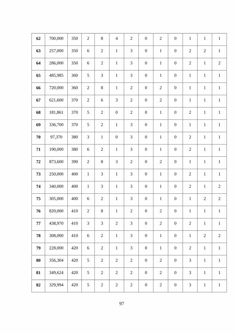
97

1 1 1 0 2 0 2 4 8 2 350 700,000 62

1 2 2 0 1 0 3 1 2 6 350 257,000 63

2 1 2 0 1 0 3 1 2 6 350 286,000 64

1 1 1 0 1 0 3 1 3 5 360 485,985 65

1 1 1 0 2 0 2 1 8 2 360 720,000 66

1 1 1 0 2 0 2 3 6 2 370 621,600 67

1 1 2 0 1 0 2 0 2 5 370 181,861 68

1 1 1 0 1 0 3 1 2 5 370 336,700 69

1 1 2 0 1 0 3 0 1 3 380 97,370 70

1 1 2 0 1 0 3 1 2 6 380 190,000 71

1 1 1 0 2 0 2 3 8 2 390 873,600 72

1 1 2 0 1 0 3 1 3 1 400 250,000 73

2 1 2 0 1 0 3 1 3 1 400 340,000 74

2 2 1 0 1 0 3 1 2 6 400 305,000 75

1 1 1 0 2 0 2 1 8 2 410 820,000 76

1 1 2 0 2 0 3 2 3 3 410 438,970 77

2 2 1 0 1 0 3 1 2 6 410 308,000 78

1 1 2 0 1 0 3 1 2 6 420 228,000 79

1 1 3 0 2 0 2 2 2 5 420 356,304 80

1 1 3 0 2 0 2 2 2 5 420 349,624 81

1 1 3 0 2 0 2 2 2 5 420 329,994 82

98

1 1 3 0 3 0 2 1 4 2 425 616,150 83

2 1 2 0 1 0 3 4 2 6 430 251,000 84

1 1 2 0 1 0 3 1 2 6 430 355,238 85

1 2 1 0 2 0 3 1 5 6 450 833,490 86

1 2 2 0 2 0 3 1 1 5 450 196,898 87

1 1 2 0 1 0 3 1 1 1 450 111,612 88

2 1 2 0 1 0 3 4 2 6 450 267,100 89

1 1 2 0 1 0 3 1 1 1 460 112,980 90

1 1 2 0 1 0 3 1 1 1 460 112,980 91

1 1 1 0 1 0 2 3 3 2 465 465,900 92

1 1 2 0 1 0 3 1 1 1 470 114,980 93

1 1 3 0 2 0 2 1 2 5 480 415,334 94

1 1 2 0 1 0 3 2 2 3 480 327,231 95

1 1 2 0 1 0 3 1 2 6 490 320,000 96

1 1 1 0 2 0 2 1 7 2 500 875,000 97

1 1 2 0 1 0 3 1 2 6 500 320,000 98

2 1 1 0 3 0 3 1 3 5 540 785,700 99

1 2 1 0 1 0 3 4 2 6 550 358,000 100

1 1 1 0 2 0 2 1 7 2 580 1,015,000 101

2 1 1 0 3 0 3 1 4 5 580 1,106,640 102

1 1 2 0 2 0 3 2 3 3 590 562,608 103

99

1 2 2 0 1 0 2 1 3 5 590 579,630 104

1 1 1 0 2 0 2 1 8 2 600 1,152,000 105

2 1 2 0 1 0 3 3 2 6 600 452,000 106

2 1 0 0 1 0 3 1 1 5 600 320,190 107

1 1 0 0 1 0 3 3 1 5 600 335,881 108

1 1 2 0 2 0 3 2 3 3 617 520,806 109

1 1 1 0 2 0 2 4 8 2 620 1,388,800 110

1 1 1 0 3 0 1 0 2 6 630 208,000 111

1 1 2 0 1 0 3 0 1 5 630 119,511 112

1 1 3 0 1 0 2 1 4 5 630 433,000 113

1 2 1 0 2 0 2 1 3 5 670 936,660 114

1 1 3 0 3 1 2 1 5 2 670 1,038,000 115

1 1 1 0 2 0 2 1 4 2 700 644,000 116

1 2 1 0 2 0 2 1 4 5 700 1,343,000 117

1 2 1 0 2 0 2 1 4 5 710 1,363,000 118

2 2 2 0 1 0 3 1 5 6 750 1,147,000 119

1 1 2 0 1 0 3 1 2 1 750 375,000 120

1 1 2 0 1 0 3 1 2 1 755 379,000 121

1 1 2 0 1 0 3 3 2 3 780 363,780 122

1 1 1 0 3 0 3 1 3 6 780 565,685 123

1 1 2 0 1 0 3 2 3 4 810 782,460 124

100

1 1 2 0 1 0 3 2 3 4 830 835,395 125

0 0 0 0 0 0 3 1 3 6 835 297,130 126

1 1 2 0 2 0 3 2 3 4 850 901,236 127

1 1 2 0 2 0 3 2 3 4 850 880,486 128

1 1 2 0 2 0 3 2 3 4 850 902,025 129

1 1 2 0 1 0 3 2 3 4 850 847,535 130

1 1 2 0 2 0 3 2 3 4 850 907,229 131

1 1 2 0 2 0 3 2 3 4 850 813,945 132

1 1 2 0 2 0 3 2 3 4 850 802,235 133

1 1 2 0 2 0 3 2 3 4 850 863,193 134

1 1 2 0 2 0 3 2 3 4 850 901,236 135

2 2 3 2 2 1 3 1 6 5 870 3,287,454 136

1 1 2 0 1 0 3 2 3 4 900 860,246 137

1 1 2 0 2 0 3 2 3 4 900 902,025 138

1 1 2 0 1 0 3 2 3 4 920 840,971 139

1 1 2 0 2 0 3 2 3 4 930 977,208 140

1 1 2 0 2 0 3 2 3 4 955 997,000 141

1 2 1 0 1 1 1 1 2 2 960 510,000 142

1 1 2 0 2 0 3 2 3 4 970 1,012,194 143

1 1 2 0 2 0 3 2 3 4 980 1,070,000 144

1 1 2 0 2 0 3 2 3 4 980 1,020,426 145

101

1 1 2 0 2 0 3 2 3 4 980 1,071,278 146

1 1 2 0 2 0 3 3 3 4 980 1,157,901 147

1 1 2 0 2 0 3 3 3 4 980 1,167,559 148

1 1 2 0 2 0 3 2 3 4 980 1,020,696 149

1 1 2 0 2 0 3 2 3 4 980 993,000 150

1 1 2 0 2 0 3 2 3 4 980 1,066,946 151

1 1 2 0 2 0 3 2 3 4 980 1,053,495 152

1 1 2 0 2 0 3 2 3 4 980 1,032,105 153

1 1 2 0 2 0 3 2 3 4 995 1,051,400 154

2 1 2 1 2 0 3 3 2 6 1000 850,000 155

2 2 2 0 1 3 2 4 7 5 1000 1,586,561 156

1 1 2 0 2 0 3 2 3 4 1020 897,143 157

1 1 2 0 1 0 2 2 3 4 1050 1,036,080 158

1 1 2 0 2 0 1 3 3 2 1070 1,050,000 159

2 2 2 1 3 0 3 4 3 6 1100 1,610,000 160

2 2 1 1 2 2 2 4 5 5 1100 2,305,000 161

1 1 1 0 2 0 1 1 4 2 1150 1,241,000 162

2 2 2 1 3 0 3 4 3 6 1170 1,681,290 163

2 2 3 1 3 2 3 1 3 5 1180 1,578,000 164

1 1 3 0 3 1 1 4 3 2 1200 1,110,000 165

2 2 1 1 2 2 2 4 4 5 1200 2,031,200 166

102

1 1 3 0 3 1 1 4 3 2 1200 1,110,000 167

2 2 1 1 2 2 2 4 4 5 1200 2,030,400 168

2 1 2 1 3 0 3 2 2 6 1200 1,149,000 169

M.Sc. Thesis Cost estimation for building construction...

Documents

Transcript of M.Sc. Thesis Cost estimation for building construction...