NAVAL POSTGRADUATE

SCHOOL

MONTEREY, CALIFORNIA

THESIS

Approved for public release; distribution is unlimited

NETTED LPI RADARS

by

Charalampos Fougias and

Charalampos Menychtas

September 2011

Thesis Advisor: Edward Fisher Second Reader: Wolfgang Baer

THIS PAGE INTENTIONALLY LEFT BLANK

i

REPORT DOCUMENTATION PAGE Form Approved OMB No. 0704-0188Public reporting burden for this collection of information is estimated to average 1 hour per response, including the time for reviewing instruction, searching existing data sources, gathering and maintaining the data needed, and completing and reviewing the collection of information. Send comments regarding this burden estimate or any other aspect of this collection of information, including suggestions for reducing this burden, to Washington headquarters Services, Directorate for Information Operations and Reports, 1215 Jefferson Davis Highway, Suite 1204, Arlington, VA 22202-4302, and to the Office of Management and Budget, Paperwork Reduction Project (0704-0188) Washington DC 20503. 1. AGENCY USE ONLY (Leave blank)

2. REPORT DATE September 2011

3. REPORT TYPE AND DATES COVERED Master’s Thesis

4. TITLE AND SUBTITLE Netted LPI RADAs 6. AUTHOR(S) Charalampos Fougias and Charalampos Menychtas

5. FUNDING NUMBERS

7. PERFORMING ORGANIZATION NAME(S) AND ADDRESS(ES) Naval Postgraduate School Monterey, CA93943-5000

8. PERFORMING ORGANIZATION REPORT NUMBER

9. SPONSORING /MONITORING AGENCY NAME(S) AND ADDRESS(ES)

N/A

10. SPONSORING/MONITORING AGENCY REPORT NUMBER

11. SUPPLEMENTARY NOTES The views expressed in this thesis are those of the authors and do not reflect the official policy or position of the Department of Defense or the U.S. Government. IRB Protocol number: N/A. 12a. DISTRIBUTION / AVAILABILITY STATEMENT Approved for public release; distribution is unlimited

12b. DISTRIBUTION CODE

13. ABSTRACT (maximum 200 words) A significant number of Low Probability of Intercept (LPI) radars are used in various military applications, from guided weapons (such anti-ship missile), to large platforms (aircrafts, ships), to large systems (Integrated Air Defense Systems – IADS). Thepurpose of this thesis is to evaluate the performance of netted LPI radar systems. To do so, it commences with establishing the theoretical background for the LPI radar techniques and detection methods. Additionally, it presents existing LPI assets along with their operational characteristics to provide the reader with a useful tool for comparative analysis of the LPI radar market. As this work focuses on LPI radar networks, specific emphasis is given to clarifying the notion of a netted system; the conceptual and mathematical background for such are presented in a separate chapter.

15. NUMBER OF PAGES

323

14. SUBJECT TERMS Networks, LPI, Radar

16. PRICE CODE

17. SECURITY CLASSIFICATION OF REPORT

Unclassified

18. SECURITY CLASSIFICATION OF THIS PAGE

Unclassified

19. SECURITY CLASSIFICATION OF ABSTRACT

Unclassified

20. LIMITATION OF ABSTRACT

UU NSN 7540-01-280-5500 Standard Form 298 (Rev. 2-89) Prescribed by ANSI Std. 239-18

ii

THIS PAGE INTENTIONALLY LEFT BLANK

iii

Approved for public release; distribution is unlimited

NETTED LPI RADARs

Charalampos Fougias Major, Hellenic Air Force

B.S., Hellenic Air Force Academy, 1995

Charalampos Menychtas Lieutenant, Hellenic Navy

B.S., Hellenic Naval Academy, 2002

Submitted in partial fulfillment of the requirements for the degree of

MASTER OF SCIENCE IN SYSTEMS ENGINEERING

from the

NAVAL POSTGRADUATESCHOOL September 2011

Authors: Charalampos Fougias Charalampos Menychtas

Approved by: Edward Fisher Thesis Advisor

Wolfgang Baer Co-Advisor

Dan Boger Chairman, Department of Information Sciences

iv

THIS PAGE INTENTIONALLY LEFT BLANK

v

ABSTRACT

A significant number of Low Probability of Intercept (LPI)

radars are used in various military applications, from

guided weapons (such anti-ship missile), to large platforms

(aircrafts, ships), to large systems (Integrated Air

Defense Systems – IADS). The purpose of the present thesis

is to evaluate the performance of netted LPI radar systems.

To do so, it commences with establishing the theoretical

background for the LPI radar techniques and detection

methods. Additionally, it presents existing LPI assets

along with their operational characteristics to provide the

reader with a useful tool for comparative analysis of the

LPI radar market. As this work focuses on LPI radar

networks, specific emphasis is given to clarifying the

notion of a netted system; the conceptual and mathematical

background for such are presented in a separate chapter.

vi

THIS PAGE INTENTIONALLY LEFT BLANK

vii

TABLE OF CONTENTS

I. INTRODUCTION ............................................1 A. BACKGROUND .........................................1 B. SCOPE OF THE THESIS ................................2 C. RESEARCH QUESTIONS .................................3 D. METHODOLOGY ........................................3 E. BENEFITS OF THE STUDY ..............................4 F. THESIS OUTLINE .....................................4

II. LPI RADAR THEORY OF OPERATION AND TECHNIQUES ............7 A. DEFINITIONS ........................................7 B. LPI RADAR EVOLUTION HISTORY ........................8 C. BASIC PRINCIPLES OF LPI RADAR OPERATION ...........11

1. Power Management .............................11 2. Waveform Shaping .............................12 3. Antenna Design ...............................14

a. Low Level Antenna Sidelobes .............14 b. Antenna Scan Patterns ...................18

4. Carrier Frequency Selection ..................19 5. High Receiver Sensitivity ....................20 6. Processing Gain of LPI Radar .................22

a. Coherent Processing .....................25 b. LPI Waveforms ...........................25

III. EXAMPLES OF AIRBORNE, MARITIME AND LAND-BASED LPI RADARS .................................................41 A. AIRBORNE LPI RADARS ...............................42

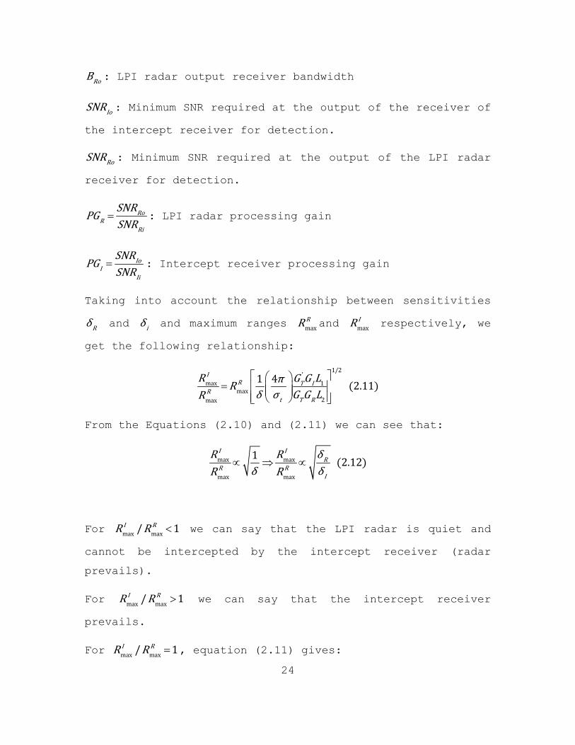
1. AN/APN-232 Combined Altitude Radar Altimeter .42 2. HG-9550 Radar Altimeter ......................42 3. GRA-2000 Radar Altimeter .....................43 4. PA-5429 Radar Altimeter ......................44 5. CMRA – Cruise Missile Radar Altimeter ........44 6. AHV-2XX0 Family of Radar Altimeters ..........45 7. AD-1990 Radar Altimeter ......................45 8. AN/APS-147 Radar .............................46 9. AN/APQ-181 Radar .............................47 10. AN/APG-77 Radar ..............................47 11. LANTIRN (Low-Altitude Navigation and

Targeting Infra-Red for Night) ...............48 12. RBS-15 Mk3 Missile Seeker ....................50

B. MARITIME LPI RADARS ...............................51 1. Pilot Radar ..................................51 2. Scout Radar ..................................52 3. Smart-L Radar ................................53 4. VARIANT Radar ................................54

viii

5. AN/SPN-46 (V) Precision Approach Landing System .......................................55

C. LAND-BASED LPI RADARS .............................55 1. TALS--Tactical Automatic Landing System ......55 2. Eagle Fire Control Radar .....................56 3. HARD-3D Radar ................................57 4. POINTER Radar ................................58 5. PAGE Radar ...................................59 6. CRM-100 Radar ................................59 7. JY-17A Radar .................................60

IV. DETECTION OF LPI RADARS ................................63 A. ES RECEIVER CHALLENGES ............................66

1. Radar Processing Gain ........................66 2. High Sensitivity Requirement .................68

B. TYPES OF ES RECEIVERS FOR LPI RADAR DETECTION .....69 1. Crystal Video Receiver .......................71 2. Instantaneous Frequency Management Receivers

(IFM) ........................................74 3. Superheterodyne Receiver .....................77 4. Channelized Receivers ........................79 5. Transform Intercept Receivers ................81 6. Cueing Systems/Hybrid Systems ................82

C. DETECTION ACCURACY ................................85 1. Detection Finding Techniques .................85

a. Rotating Directional Antenna ............85 b. Multiple Antenna Amplitude Comparison ...85 c. Watson Watt .............................86 d. Doppler .................................86 e. Interferometer ..........................86 f. Amplitude Angle of Arrival ..............87 g. Phase Angle of Arrival ..................91

2. Precision Emitter Location Techniques ........92 a. Time Difference of Arrival (TDOA) .......93 b. Frequency Difference of Arrival (FDOA) ..96

D. SIGNAL PROCESSING ALGORITHMS ......................98 1. Wigner Ville Distribution (WVD) .............100 2. Choi Williams Distribution ..................103

V. JAMMING METHODS FOR LPI RADARS ........................107 A. CONCEPTUAL CLARIFICATIONS ........................107

1. EA Radar Jamming Waveforms ..................107 2. LPI Jamming Probability: The Issue of

Interception ................................108 B. LPI RADAR JAMMER DESIGN REQUIREMENTS .............111

1. Bandwidth ...................................111 2. Radar Receiver Sensitivity Advantage ........113

ix

C. ANTIJAM ADVANTAGE OF LPI .........................115 D. JAMMING ..........................................117

1. FSK .........................................117 2. PSK .........................................118 3. FMCW ........................................119

VI. NETWORKS AND NETCENTRIC WARFARE (NCW) .................125 A. INTRODUCTION .....................................125 B. NETWORK-CENTRIC WARFARE ..........................125 C. NCW REQUIREMENTS .................................126

1. Situational Awareness .......................128 2. Maneuverability .............................128 3. Decision Speed and Operational Tempo ........129 4. Agility .....................................130 5. Lethality ...................................131

D. METRICS FOR INFORMATION GRID ANALYSIS ............131 1. Generalized Connectivity Measure ............132 2. Reference Connectivity Measure ..............133 3. Network Reach ...............................133 4. Extended Generalized Connectivity Measure ...134 5. Entropy and Network Richness ................135

a. Entropy ................................135 b. Network Richness .......................138

6. Maximum Operational Tempo ...................139 7. Example .....................................141

E. NETTED LPI RADAR SYSTEMS .........................150 VII. NETTED RADAR SYSTEMS -- ADVANTAGES AND DISADVANTAGES .153

A. MULTISITE RADAR SYSTEMS CATEGORIZATION ...........153 1. Type of Targets of Interest .................153 2. The Degree of Spatial Coherence .............154

a. Spatially Coherent MSRSs ...............154 b. Short-Term Spatial Coherent MSRSs ......154 c. Spatially Incoherent MSRSs .............155

3. Information Fusion Level ....................157 a. Radio Signal Integration Level .........157 b. Video Signal Integration Level .........157 c. Plot Integration Level .................157 d. Track Integration Level ................158

4. Degree of Autonomy of Signal Reception ......159 a. Independent (Autonomous) Signal

Reception ..............................159 b. Cooperative Signal Reception ...........160 c. Independent - Cooperative Signal

Reception ..............................160 5. Station Location and Mobility ...............160

x

a. Ground-Based MSRSs With Stationary Stations ...............................160

b. Ground-based MSRSs With Mobile Stations 160 c. Transmitter (or Receiver) on Platforms,

Receiver (or Transmitter) Ground-based. 160 d. All Stations on Platforms ..............161 e. Shipborne ..............................161

B. ADVANTAGES OF MULTISITE RADAR SYSTEMS ............161 1. Capability to Form Coverage Area of Required

Configuration for Expected Environments .....161 2. Power Advantages ............................161 3. Detection of Stealth Targets ................162 4. High Accuracy of the Position Estimation of

a Target ....................................162 5. Possibility of Estimating Target’s Velocity

and Acceleration Vectors by the Doppler Method ......................................164

6. Capability to Measure Three Coordinates and Velocity Vector of Radiation Sources ........167

7. Increase of Resolution Capability ...........168 8. Increase of Target Handling Capacity ........171 9. Increase of “Signal Information” Body .......172 10. Increase of Jamming Resistance ..............172

a. Resistance to Sidelobe Jamming .........173 b. Resistance to Main Lobe Jamming ........173

11. Increase of Clutter Resistance ..............174 12. Increase of Survivability and Reliability ...175 13. Technical and Operational Advantages ........176 14. Detection of Non-LOS Targets ................176

C. DISADVANTAGES OF MULTISITE RADAR SYSTEMS .........177 1. Centralized Control of Spatially Separate

Stations ....................................177 2. Necessity of Data Transmission Conduits .....177 3. Additional Requirements for Synchronization,

Phasing of Spatially Separate Stations, Transmission of Reference Frequencies and Signals .....................................178

4. Increased Requirements to Signal and Data Processors and Computer Systems .............179

5. Necessity for Accurate Station Positioning and Mutual Alignment ........................179

6. Need for Direct LOS Between Stations and Targets .....................................180

7. High Cost ...................................180 D. SUMMARY ..........................................181

VIII.SIMULATION SCENARIO ...................................185

xi

A. SCENARIO 1: 1 SSJ ................................193 1. Scenario 1 Time Index 1 .....................193

a. `SNR – Non-Netted ......................193 b. `SNR – Netted ..........................194 c. `JSR – Non-Netted ......................195 d. `JSR – Netted ..........................196 e. `S/(J+N) – Non-Netted ..................197 f. S/(J+N) – Netted .......................198

2. Scenario 1 Time index 2 (5 LPI Radar + 1 SSJ) ........................................199 a. SNR Non-Netted .........................199 b. SNR Netted .............................200 c. JSR Non-Netted .........................201 d. JSR Netted .............................202 e. S/(J+N) Non-Netted .....................203 f. S/(J+N) Netted .........................204

3. Scenario 1 Time index 3 (5 LPI Radar + 1 SSJ) ........................................205 a. SNR – Non-Netted .......................205 b. SNR –Netted ............................206 c. JSR – Non-Netted .......................207 d. JSR – Netted ...........................208 e. S/(J+N) – Non-Netted ...................209 f. S/(J+N) –Netted ........................210

Β. SCENARIO 2: 1 STAND-OFF JAMMER & 1 TARGET ........211 1. Scenario 2 Time Index 1 .....................211

a. SNR – Non-Netted .......................211 b. SNR – Netted ...........................212 c. JSR – Non-Netted .......................213 d. JSR –Netted ............................214 e. S/(J+N) – Non-Netted ...................215 f. S/(J+N) –Netted ........................216

2. Scenario 2 Time Index 2 .....................217 a. SNR – Non-Netted .......................217 b. SNR –Netted ............................218 c. JSR – Non-Netted .......................219 d. JSR –Netted ............................220 e. S/(J+N) – Non-Netted ...................221 f. S/(J+N) –Netted ........................222

3. Scenario 2 Time Index 3 .....................223 a. SNR – Non-Netted .......................223 b. SNR –Netted ............................224 c. JSR – Non-Netted .......................225 d. JSR –Netted ............................226 e. S/(J+N) – Non-Netted ...................227 f. S/(J+N)– Netted ........................228

xii

C. SCENARIO 3: 2 STAND IN JAMMERS ...................229 1. Scenario 3 Time Index 1 .....................229

a. SNR – Non-Netted .......................229 b. SNR – Netted ...........................230 c. JSR – Non-Netted .......................231 d. JSR –Netted ............................232 e. S/(J+N) – Non-Netted ...................233 f. S/(J+N)- Netted ........................234

2. Scenario 3 Time Index 2 .....................235 a. SNR – Non-Netted .......................235 b. SNR – Netted ...........................236 c. JSR – Non-Netted .......................237 d. JSR – Netted ...........................238 e. S/(J+N) – Non-Netted ...................239 f. S/(J+N)–Netted .........................240

3. Scenario 3 Time Index 3 .....................241 a. SNR – Non-Netted .......................241 b. SNR –Netted ............................242 c. JSR – Non-Netted .......................243 d. JSR –Netted ............................244 e. S/(J+N) – Non-Netted ...................245 f. S/(J+N) –Netted ........................246

IX. CONCLUSIONS ...........................................253 APPENDIX. DETAILED DESCRIPTION OF PHASE MODULATING

TECHNIQUES, FREQUENCY SHIFT KEYING TECHNIQUES AND NOISE TECHNIQUES ......................................257 A. PHASE MODULATING TECHNIQUES ......................257

1. BPSK Codes ..................................257 2. Polyphase Codes .............................260

a. Polyphase Barker Codes .................260 b. Frank Code .............................261 c. P1 Code ................................263 d. P2 Code ................................265 e. P3 Code ................................267 f. P4 Code ................................269

3. Polytime Codes ..............................271 a. T1(n) ..................................271 b. T2(n) ..................................273 c. T3(n) ..................................275 d. T4(n) ..................................277

B. FREQUENCY SHIFT KEYING (FSK) TECHNIQUES ..........279 1. Costas Codes ................................279 2. Hybrid FSK/PSK Technique ....................281 3. Matched FSK/PSK Technique ...................283

C. NOISE TECHNIQUES .................................284

xiii

1. RNR .........................................284 2. RNFR ........................................285 3. RNFSR .......................................286 4. RBPC ........................................287

LIST OF REFERENCES .........................................289 INITIAL DISTRIBUTION LIST ..................................295

xiv

THIS PAGE INTENTIONALLY LEFT BLANK

xv

LIST OF FIGURES

Figure 1. Pulse Compression...............................13 Figure 2. FMCW............................................14 Figure 3. Conventional (a) and Low Sidelobe Antenna

Patterns (b)....................................18 Figure 4. Atmospheric Attenuation vs Frequency............20 Figure 5. Linear FMCW Triangular Waveform.................28 Figure 6. Linear FMCW In-Phase Ramp-up Signal.............31 Figure 7. AN/APN-232......................................42 Figure 8. HG9550..........................................43 Figure 9. GRA-2000........................................44 Figure 10. AHV-2XX0 Family of Radar Altimeters.............45 Figure 11. AN/APS-147 Radar (Antenna Under Helicopter

Cockpit--Red Arrow).............................46 Figure 12. AN/APG-77 Radar Antenna.........................48 Figure 13. LANTIRN Pods on F-16--Red Arrows................50 Figure 14. AN/AAQ-13 Navigation Pod........................50 Figure 15. Pilot Radar on Visby-class Corvette (Radar

Antenna--Red Arrow).............................52 Figure 16. Scout Radar.....................................53 Figure 17. Smart-L Radar...................................54 Figure 18. VARIANT Radar...................................54 Figure 19. AN/SPN-46 (V)...................................55 Figure 20. TALS............................................56 Figure 21. Eagle Fire Control Radar........................57 Figure 22. HARD-3D Radar...................................58 Figure 23. Pointer Radar...................................58 Figure 24. PAGE Radar......................................59 Figure 25. CRM-100.........................................60 Figure 26. CVR Block Diagram...............................71 Figure 27. IFM Principle...................................74 Figure 28. Digital Multioctave IFM Block Diagram...........76 Figure 29. Digitally Controlled Superheterodyne Receiver

Block Diagram...................................77 Figure 30. AN/ALR-56M Radar Warning Receiver (RWR).........79 Figure 31. Channelized Intercept Receiver Block Diagram....80 Figure 32. Hybrid Receiver Block Diagram...................82 Figure 33. Broadband Cavity Backed Spiral Gain Pattern.....88 Figure 34. Amplitude AOA Pattern Displacement..............88 Figure 35. Angle of Arrival Measurement by Amplitude

Comparison......................................89 Figure 36. Phase Comparison AOA Measurement................91 Figure 37. Isochrone Lines; Two Aircraft Time Difference

of Arrival......................................94

xvi

Figure 38. Isochrone Lines; Two Aircraft Time Difference of Arrival......................................94

Figure 39. The Anti-jam Advantage of LPI Communication....116 Figure 40. The Bit Error Rate in a Digital Receiver Cannot

Exceed 50 Percent; a 0dB JSR Reaches this Level of Errors;.....................................117

Figure 41. Relationship Between Network Space and Challenges.....................................127

Figure 42. Maneuverability................................129 Figure 43. OODA Loop......................................129 Figure 44. Operational Tempo vs. Force Agility............130 Figure 45. Three-node Network Example.....................134 Figure 46. Time Spent in Each OODA Cycle Phase............140 Figure 47. Network Topology...............................142 Figure 48. Network Topology after EA......................147 Figure 49. Three-node MIMO Netted Radar System............151 Figure 50. Netted Mono-static (left) Multi-static (right)

Increase of Angular Coordinate Measurement Accuracy.......................................163

Figure 51. Netted Mono-static (left) Multi-static (right) Target Velocity Vector Measurement by the Doppler Method.................................165

Figure 52. Angular Resolution of MSRS.....................168 Figure 53. Simulation Network Topology....................185 Figure 54. Non-Netted SNR Contour Chart at Time Index=1...193 Figure 55. Netted SNR Contour Chart at Time Index=1.......194 Figure 56. Non-netted JSR Contour Chart at Time Index=1...195 Figure 57. Netted JSR Contour Chart at Time Index=1.......196 Figure 58. Non-netted SNJR Contour Chart at Time Index=1..197 Figure 59. Netted SNJR Contour Chart at Time Index=1......198 Figure 60. Non-netted SNR Contour Chart at Time Index=2...199 Figure 61. Netted SNR Contour Chart at Time Index=2.......200 Figure 62. Non-netted JSR Contour Chart at Time Index=2...201 Figure 63. Netted JSR Contour Chart at Time Index=2.......202 Figure 64. Non-netted SNJR Contour Chart at Time Index=2..203 Figure 65. Netted SNJR Contour Chart at Time Index=2......204 Figure 66. Non-netted SNR Contour Chart at Time Index=3...205 Figure 67. Netted SNR Contour Chart at Time Index=3.......206 Figure 68. Non-netted JSR Contour Chart at Time Index=3...207 Figure 69. Netted JSR Contour Chart at Time Index=3.......208 Figure 70. Non-netted SNJR Contour Chart at Time Index=3..209 Figure 71. Netted SNJR Contour Chart at Time Index-3......210 Figure 72. Non-netted SNR Contour Chart at Time Index=1...211 Figure 73. Netted SNR Contour Chart at Time Index=1.......212 Figure 74. Non-netted JSR Contour Chart at Time Index=1...213 Figure 75. Netted JSR Contour Chart at Time Index=1.......214

xvii

Figure 76. Non-netted SNJR Contour Chart at Time Index=1..215 Figure 77. Netted SNJR Contour Chart at Time Index=1......216 Figure 78. Non-netted SNR Contour Chart at Time Index=2...217 Figure 79. Netted SNR Contour Chart at Time Index=2.......218 Figure 80. Non-netted JSR Contour Chart at Time Index=2...219 Figure 81. Netted JSR Contour Chart at Time Index=2.......220 Figure 82. Non-netted SNJR Contour Chart at Time Index=2..221 Figure 83. Netted SNJR Contour Chart at Time Index=2......222 Figure 84. Non-netted SNR Contour Chart at Time Index=3...223 Figure 85. Netted SNR Contour Chart at Time Index=3.......224 Figure 86. Non-netted JSR Contour Chart at Time Index=3...225 Figure 87. Netted JSR Contour Chart at Time Index=3.......226 Figure 88. Non-netted SNJR Contour Chart at Time Index=3..227 Figure 89. Netted SNJR Contour Chart at Time Index=3......228 Figure 90. Non-netted SNR Contour Chart at Time Index=1...229 Figure 91. Netted SNR Contour Chart at Time Index=1.......230 Figure 92. Non-netted JSR Contour Chart at Time Index=1...231 Figure 93. Netted JSR Contour Chart at Time Index=1.......232 Figure 94. Non-netted SNJR Contour Chart at Time Index=1..233 Figure 95. Netted SNJR Contour Chart at Time Index=1......234 Figure 96. Non-netted SNR Contour Chart at Time Index=2...235 Figure 97. Netted SNR Contour Chart at Time Index=2.......236 Figure 98. Non-netted JSR Contour Chart at Time Index=2...237 Figure 99. Netted JSR Contour Chart at Time Index=2.......238 Figure 100. Non-netted SNJR Contour Chart at Time Index=2..239 Figure 101. Netted SNJR Contour Chart at Time Index=2......240 Figure 102. Non-netted SNR Contour Chart at Time Index=3...241 Figure 103. Netted SNR Contour Chart at Time Index=3.......242 Figure 104. Non-netted JSR Contour Chart at Time Index=3...243 Figure 105. Netted JSR Contour Chart at Time Index=3.......244 Figure 106. Non-netted SNJR Contour Chart at Time Index=3..245 Figure 107. Netted SNJR Contour Chart at Time Index=3......246 Figure 108. Figure BPSK Modulation.........................257 Figure 109. BPSK Signal Modulated by Barker Code (length 7)259 Figure 110. Frank Code Phase...............................262 Figure 111. Signal Phase (Modulated by Frank Code).........262 Figure 112. P1 Code Phase..................................264 Figure 113. Signal Phase (Modulated by P1 Code)............264 Figure 114. P2 Code Phase..................................266 Figure 115. Signal Phase (Modulated by P2 Code)............266 Figure 116. P3 Code Phase..................................268 Figure 117. Signal Phase (Modulated by P3 Code)............268 Figure 118. P4 Code Phase..................................270 Figure 119. Signal Phase (Modulated by P4 Code)............270 Figure 120. T1(2) Stepped Frequency Phase..................272 Figure 121. T1(2) Modulated Signal Time Domain Waveform....272

xviii

Figure 122. T2(2) Stepped Frequency Phase..................274 Figure 123. T2(2) Modulated Signal Time Domain Waveform....274 Figure 124. T3(2) Stepped Frequency Phase..................276 Figure 125. T3(2) Modulated Signal Time Domain Waveform....276 Figure 126. T4(2) Stepped Frequency Phase..................278 Figure 127. T4(2) Modulated Signal Time Domain Waveform....278 Figure 128. I Channel PSD with Noise SNR=0dB...............280 Figure 129. I Channel PSD with No Noise....................280 Figure 130. FSK (Costas Only) PSD..........................282 Figure 131. Hybrid FSK (Costas)/PSK (Barker) PSD...........283

xix

LIST OF TABLES

Table 1. Phase Modulating Techniques Advantages/ Disadvantages...................................34

Table 2. Phase Modulating Techniques Advantages /Disadvantages..................................37

Table 3. Noise Techniques Advantages/Disadvantages.......39 Table 4. Examples of LPI Radars..........................41 Table 5. Intercept Receiver Typical Performance..........70 Table 6. Typical ES Receivers' Performance Parameters....84 Table 7. Typical Deployed Intercept Receivers...........106 Table 8. Modern EA Systems..............................123 Table 9. Degree of Spatial Coherence Summary............156 Table 10. Information Fusion Level Summary...............159 Table 11. Summary of MSRS Advantages for Types of MSRSs..183 Table 12. Summary of MSRS Disadvantages for Types of

MSRSs..........................................184 Table 13. LPI Radar & Target Characteristics.............186 Table 14. Maximum Detection Range vs. Intercept

Receiver’s Sensitivity.........................191 Table 15. Summary of Simulation Results..................247 Table 16. Barker Codes...................................258 Table 17. Compound Barker Code for 4cN = ..................258

xx

THIS PAGE INTENTIONALLY LEFT BLANK

xxi

LIST OF ACRONYMS AND ABBREVIATIONS

ALCM: Air Launched Cruise Missile

AOA: Angle of Arrival

AOR: Area of Regard

AWGN: Additive White Gaussian Noise

ARM: Anti-Radiation Missile

BPSK: Binary Phase Shift Keying

CVR: Crystal Video Receiver

CW: Continuous Wave

CWD: Choi-Williams Distribution

DECM: Deceptive Electronic Countermeasures

DOA: Direction of Arrival

DoD: Department of Defense

EA: Electronic Attack

ECM: Electronic Countermeasures

ELINT: Electronic Intelligence

EP: Electronic Protection

ES: Electronic Support

ESM: Electronic Support Measure

EW: Electronic Warfare

FDOA: Frequency Direction of Arrival

FH: Frequency Hopping

FLIR: Forward Looking Infra-Red

FM: Frequency Modulation

FMCW: Frequency Modulation Continuous Wave

FOV: Field of View

FSK: Frequency Shift Keying

HPBW: Half-Power Beamwidth

IADS: Integrated Air-Defense System

IFF: Identification of Friend or Foe

IFM: Instantaneous Frequency Management

xxii

IR: Infra-Red

ISAR: Inverse Synthetic Aperture Radar

JSR: Jamming to Signal Ratio

LAN: Local Area Network

LPI: Low Probability of Intercept

MIMO: Multiple-Input Multiple-Output

MSRS: Multiple Radar System

MTI: Moving Target Indicator

NCW: Net-centric Warfare

OODA: Observation- Orientation- Decision- Action

OTHT: Over the Horizon Targeting

POI: Probability of Intercept

PSD: Power Spectral Density

PSK: Phase Shift Keying

PSL: Peak Sidelobe

QMFB: Quadrature Mirror Filter Bank

RBPC: Random Binary Phase Code

RCS: Radar Cross-Section

RF: Radio Frequency

RMS: Root Mean Square

RNFR: Random Noise Radar plus FMCW

RNFSR: RNFR plus sine

RNR: Random Noise Radar

RWR: Radar Warning Receiver

SAR: Synthetic Aperture Radar

SEI: Specific Emitter Identification

SIGINT: Signal Intelligence

SNR: Signal-to-Noise Ratio

SNJR: Signal to Noise and Jamming Ratio

SOJ: Stand-Off Jamming

SSJ: Self-Screening Jamming

STC: Sensitivity Time Control

xxiii

STFT: Short-Time Fourier Transform

TDOA: Time Difference of Arrival

UV: Ultra Violet

WVD: Wigner-Ville Distribution

xxiv

THIS PAGE INTENTIONALLY LEFT BLANK

xxv

ACKNOWLEDGMENTS

Charalampos Fougias Acknowledgments:

I would like to thank all people who have helped and

inspired me during my thesis study.

First of all, I would like to extend my utmost

gratitude to my advisors Mr. Edward Fisher and Dr. Wolfgang

Baer for their valuable guidance, mentorship and monumental

patience. They were always accessible and willing to help

with my research.

Mr. Edward Fisher deserves special thanks because I

had the fortune to take one of his classes, and during that

class I was inspired to explore this area of study.

A special thanks to my “brother-in-arms” in this

thesis, Charalampos Menychtas, for his contributions,

timeless investment, and commitment to this thesis.

I would like to thank the Hellenic Air Force for

providing me the opportunity to study at the Naval

Postgraduate School.

I would also like to thank my parents for providing me

countless opportunities and for fostering a learning

environment in which ethos integrity, discipline and hard

work measure one’s potential to achieve.

To my wife, Arieta, thank you for blessing me with

unconditional love and unending support throughout my

career and especially here at Monterey, California far away

from family and friends. Few, if any, men share my luck.

xxvi

To my daughter, Kalia, thank you for bringing me such

joy and inspiration to keep going.

Last, I would like to dedicate this thesis to my wife

Arieta and my daughter Kalia.

Charalampos Menychtas Acknowledgments:

I would like to thank the Hellenic Navy for giving me

the opportunity to compete for, and earn postgraduate

education at the Naval Postgraduate School. My studies in

this institution have broadened my horizons both as an

officer and as an individual and have asserted my view that

knowledge is the most powerful weapon.

I am deeply indebted to the NPS faculty, which

willingly assisted my academic inquiries and pursuits

throughout my studies. Among the various professors I had

the honor of being taught by, my thesis advisors, Mr.

Edward Fisher and Dr. Wolfgang Baer, deserve the greatest

of appreciation for their insightful comments and

continuous support that made this project feasible.

I would also like to express my acknowledgements to

Major Fougias, for his contribution and fruitful

cooperation on this thesis work.

This work is dedicated to my family.

1

I. INTRODUCTION

A. BACKGROUND

The “classic” situation between radar and intercept

receivers has been that the latter has no difficulty

detecting and jamming the radar, and even sometimes its

sidelobes, at long ranges. To counter that performance

degradation, radar engineering is focused in concealing the

radar emissions from the adversary (the analogy of that

situation, at the target level, is to have low target Radar

Cross Section [RCS] to achieve minimal returns to the radar

receiver, to adopt special tactics to avoid detection,

etc.). Several radar techniques have been developed to

conceal radar from intercept receivers: power management,

wide operational bandwidth, frequency agility, antenna

sidelobe reduction, and advanced scan patterns

(modulations). The types of radars that utilize such

techniques are called Low Probability of Intercept (LPI)

radars.

In this “Radar versus Jammer” game, both sides have

exhibited remarkable adaptability: the jammer industry has

replied with more sophisticated intercept receivers that

try to match the LPI radar processing gain. As a response,

an increasing number of LPI radars are incorporated into

integrated air defense systems, IADS modern platforms, and

weapons, such as anti-ship missiles and littoral weapon

systems. The next step to improve the EP aspect of such

systems is to associate a number of LPI assets in a net

centric sense.

2

Examining the effect of modern jammers in net centric

vs. non-centric IADS, we can draw useful conclusions on the

effectiveness of the former: is there a comparative

advantage of such a system vs. a non-netted one? And if

there is, can it be evaluated?

B. SCOPE OF THE THESIS

This thesis provides a comprehensive volume of two

major elements in Electronic Warfare: LPI technology and

network configurations. Although the existing literature

dealing individually with LPI technology is not only wide

but also constantly updated (Lee 1991, McRitchie and

McDonald 1999, Kadambe and Adali 1998, Burgos-Garcia et al.

2000,D. Adamy 2001, Baker and Hume 2001, Skolnik 2001, Gau

2002, Lynch Jr. 2004, Wiley 2006,Pace 2009), scholarly

efforts providing insights in network configurations of

such assets is, by comparison, less extensive. In this

context, this thesis intends to fill this literature gap

and provide a more comprehensive volume covering both

academic realms on the same work.1

To do so, it commences with establishing the

theoretical background for LPI radar techniques and

detection methods. Additionally, it presents the existing

LPI assets along with their operational characteristics,

thus providing the reader with a useful tool for

comparative analysis of the LPI radar market. As this works

1 The 2008 paper of Chen and Pace presents a basic framework for

simulation of network enabled radar systems, but, apart from being limited in breadth, its scope is limited in the evaluation of the jamming effect in general radar topology. Y. Q. Chen and Phillip E. Pace, “Simulation of Information Metrics to Assess the Value of Networking in A General Battlespace Topology,” in Proc. of the IEEE International Conf. on System of Systems Engineering (IEEE, June 2008).

3

intends to elucidate the concept of LPI networks, special

emphasis shall be given to clarifying the notion of a

netted system; the theoretical and mathematical background

of such is presented in a separate chapter.

C. RESEARCH QUESTIONS

Primary:

What is the jamming effect on a netted LPI radar-based

IADS versus non-netted IADS?

Secondary:

What is LPI radar and how does it gain its advantage?

What is netted radar network and how does it gain its

advantage?

How are LPI radars most effectively netted?

How effective is EA on LPI netted networks?

D. METHODOLOGY

The methodology used in this thesis research will

consist of the following steps.

Articles, books, periodicals, thesis, IEEE, and DoD

documents related to the subject will be collected and

thoroughly examined. MATLAB simulation regarding the IADS

configuration under evaluation shall be applied to assist

the comprehensive aspect of the thesis. With the MATLAB

simulation, we will design an LPI IADS system that can be

operated in netted or autonomous configuration, and we will

examine its overall behavior under different jamming

operational techniques. The answers to questions stated in

4

the above section will be established in a reasonable

fashion.

E. BENEFITS OF THE STUDY

The results of this thesis will be used to support

ongoing efforts by the Hellenic Armed Forces. This thesis

will enhance the perspective and knowledge of Electronic

Warfare officers, related project officers, and technical

personnel. The comprehensive approach of the LPI concept

attempted in this paper will assist the Hellenic Armed

Forces in evaluating future needs and requirements of

Electronic Warfare systems on both netted and non-netted

configurations.

F. THESIS OUTLINE

The thesis research and findings are organized in the

following manner:

Chapter I comprises the introductory section of the

thesis.

Chapter II describes the LPI radar theory of operation

and techniques (waveforms, modulation) used in this thesis

work. It gives to the reader the theoretical basis of the

LPI radar operation.

Chapter III presents the airborne, maritime, and land-

based LPI radars available in the industry.

Chapter IV describes detection methods of LPI radars.

For this purpose EP receivers and signal processing

algorithms are examined in detail. Examples of EP receiver

systems used in real operational environments are also

given.

5

Chapter V discusses jamming methods for LPI radars.

Chapter VI introduces the idea of networks and

attempts to clarify the concept of net-centric warfare

(NCW).

Chapter VII looks more specifically into netted LPI

Radar Systems, addressing their advantages and

disadvantages.

Chapter VIII employs simulation of selected net

centric IADS configuration via MATLAB.

Finally, conclusions are summarized in Chapter IX.

6

THIS PAGE INTENTIONALLY LEFT BLANK

7

II. LPI RADAR THEORY OF OPERATION AND TECHNIQUES

The objective of this chapter is to enlighten the

reader about the applicable techniques for LPI radar

systems as well as to give some examples of airborne,

maritime and land-based LPI radar systems.

A. DEFINITIONS

In today’s battlefield, radar faces many threats from

Electronic Attack (EA) and Anti-Radiation Missiles (ARMs).

This situation brought about the need for the radar to try

to “see” the target without enabling the target’s passive

intercept receiver and/or other enemies’ intercept receiver

(not on board the target) to intercept the radar’s signal.

To answer that need, radars were developed that apply

various LPI techniques. These radars are called LPI radar.

LPI radar is one form of RF Stealth. It tries to hide

one’s RF emissions, or its active signature, by

implementing various techniques such as using very low

signal levels and/or specially constructed waveforms (those

will be analyzed later in this thesis).

Active signature is defined as all the observable

emissions from a platform: acoustic, chemical (soot and

contrails), communications, radar, IFF, IR, laser, and

Ultra-Violet (UV) (Lynch 2004, 3).

Radar signature reduction requires the use of various

techniques that can minimize the radar’s radiated power

density at possible intercept receiver locations. The role

of tactics is also important when one wants to minimize

8

radar’s active signature because by correct and thoughtful

tactics implementation one can reduce significantly

exposure time during emission.

B. LPI RADAR EVOLUTION HISTORY

The “classic” situation between radar and intercept

receivers has been that the intercept receiver has no

difficulty detecting the radar, and even sometimes its

sidelobes, at long ranges. That happens because the radar

transmitted wave has to “travel” twice the distance—from

radar to target (intercept receiver) and back—for the radar

to detect the target. In the case of the intercept receiver

onboard the target, the wave has to travel only the “one

way” (Skolnik 2001, 7). That can easily be seen by the

following range equations for radar versus intercept

receiver (ESM):

( )2 2

3 42.1

4RDR T T tR

RDR

P G λ σPπ R

=

2

2 2 2.24ESM T T RR

ESM

P G G λP π R=

Where:

TP = Transmitter Power

TG = Gain of RADAR Ant

RDRRP = RADAR received signal power

ESMRP = ESM received signal power

λ = Wavelength

9

tσ = Target’s RADAR Cross Section (RCS)

RG = Gain of ESM Receiver Ant

RDRR = RADAR detection range

ESMR = Intercept’s receiver detection range

From the above equations we can clearly see that the

RADAR received signal power is proportional to 41/ RDRR whereas the intercept received signal power is proportional

to 21 / ESMR . So the considering all other factors between

RADAR and intercept receiver the same or comparable

(atmospheric losses, processing gains of both receivers

etc) the path loss ( 21 / ESMR versus 41/ RDRR ) created a great

advantage for the intercept receiver.

The increased signal processing gain obtainable from

radar has given radar the potential ability to alter that

balance, on the assumption that the intercept receiver

cannot duplicate the radar’s processing gain.

LPI radar is designed to be difficult to detect by

passive radar detection equipment (such as a radar warning

receiver (RWR) or other ESM equipment) while it is

searching for or tracking a target. This characteristic is

desirable because it allows finding and tracking an

opponent without alerting them to the radar's presence.

LPI radars are generally transmitting weak signals

that the intercept receiver has difficulty detecting above

its threshold.

Many combined features help the LPI radar prevent its

detection by modern intercept receivers. These features are

10

centered on the antenna (antenna pattern and scan

patterns), the transmitter radiated waveform and LPI radar

power management features.

The capability of LPI radar to stay undetected heavily

depends upon the intercept receiver’s characteristics and

vice versa. So in order to understand LPI radars we must

understand the nature of the ESM receivers. The purpose of

an ESM receiver is to detect, sort and classify an unknown

radar (Lynch 2004, 11).

The ESM receiver achieves the detection of the radar

signal by having the necessary sensitivity and processing

power to detect a signal of specific power over a given

distance.

Sorting is the task of separating different emitters,

in a dense signal environment where many signals in

different or the same frequency band from various

directions are intercepted, so that they can then be

classified.

Classification is the task of identifying emitter type

(or even the specific emitter) and determining the

respective weapon system that the emitter is carried on.

LPI radar uses continuous wave (CW), wide bandwidth,

low power signals on the order of a few watts (or even

lower in the order of magnitude of mWatts) making its

detection difficult. Unlike conventional radars, which emit

high-energy pulses in a narrow frequency band, LPI radar

11

emits low energy pulses over a wide frequency band.

Wideband CW techniques include:

• Linear and nonlinear frequency modulation (FMCW)

• Phase modulation (Bi-phase codes such as Barker Code,

poly-phase codes such as Frank, P1, P2, P3 and P4 Code).

• Frequency hopping (FSK, Costas sequence FSK

technique).

• LPI signals are typically modulated by a periodic

function such as Barker Code, Frank Code, P1 Code, P2 Code,

P3 Code and P4 Code.

The purpose of this modulation is to generate a

“unique” waveform signature that can be detected by the

radar receiver when scattered back at very low S/N levels.

C. BASIC PRINCIPLES OF LPI RADAR OPERATION

Various features and techniques can be implemented

with radar to reduce its active signature, make it an LPI

radar and ultimately prevent its detection by modern

intercept receivers.

1. Power Management

Power management is the ability to control the power

level emitted by the antenna, and limit the power to the

appropriate range/radar Cross Section (RCS) detection

requirement (Pace 2009, 16).

The idea is that since most intercept receivers would

expect an increase in received power by the radar as the

distance decreases, the ability of the LPI radar to adjust

its radiated power to lower levels as the target approaches

12

can make the intercept receiver change its priorities for

Electronic Attack (EA) on the LPI radar.

From the LPI radar’s point of view, as can be seen in

equation 2.1, as the distance from the target is decreasing

RDRR , the LPI radar by trying to keep the level of its

received power scattered back from the target RDRRP close to

its minimum discernable level, with all other factors the

same, reduces its radiated power level TP .

From the intercept receiver’s point of view, as can be

seen in equation 2.2, by decreasing the radiated power TP

with all other factors the same (including the distance

between LPI radar and intercept receiver), the received

power by the intercept receiver ESMRP decreases, which in turn

is translated by the intercept receiver as an increase of

the distance between the LPI radar and the intercept

receiver.

2. Waveform Shaping

Conventional RADARs use waveforms comprised of pulse

trains that have a very high peak power TP and a low duty

cycle /ave TDC P P= . These kinds of waveforms are easily

detectable by intercept receivers. Since the detection of a

target relies upon the total back scattered power to the

radar receiver, modern radar use special waveforms that:

• Disperse the power of one pulse in many pulses (that

will hit the same target) and integrate them together

(coherently or non-coherently) taking their added effect,

as we can see in Figure 1. That is pulse compression (for

13

pulsed radar) and is based on the fact that what matters to

radar detection is the total amount of energy reflected

back from the target.

Figure 1. Pulse Compression

• Disperse the power in low energy pulses over a wide

frequency band, as we can see in Figure 2. That can be done

by using a CW waveform properly modulated by techniques

mentioned earlier. This is the main technique used in LPI

radar that uses FM modulation ramps, but as we reported

previously there are other types of modulating the CW wave

used at an LPI radar. LPI radar has low TP but high aveP .

14

Figure 2. FMCW

In general, waveform shaping techniques provide the

extra processing gain that gives radar its main advantage

with respect to ESM receivers, but it also forms a power

management “like” method to reduce the peak power of the

radar.

3. Antenna Design

a. Low Level Antenna Sidelobes

Radar applications generally demand low sidelobe

antennas for the following reasons, which are also the

advantages of achieving low sidelobes (Lynch 2004, 354):

• If the sidelobes are large enough, they

radiate a large portion of the total radiated energy of the

antenna. That fact would cause a reduction of the main beam

energy and consequently the decrease of the antenna gain.

• Low sidelobes reduce clutter returns (they

cover most of the space around the antenna, and since the

antenna is pointing at the point of interest, their returns

are mostly unwanted clutter).

15

• Low sidelobes reduce interference (mostly

from nearby friendly transmitters).

• Low sidelobes reduce ECM susceptibility and

probability of intercept (high levels of sidelobes make

jamming easier and, since they cover most of the space

around the antenna, can expose it easily at various

bearings).

Typical sidelobe levels for conventional radar

are around -20 dB whereas for LPI radar the acceptable

level is around -45 dB (Pace 2009, 8). It is rather easy to

manufacture antennas with sidelobe levels of –35 to –40 dB,

and with extreme care it is possible to go even lower (–50

or –55 dB). However, considerably lower sidelobes are

difficult to achieve, primarily as a result of

manufacturing tolerances (Lynch 2004, 354).

One other effect of the ultra-low sidelobe

antenna, apart from the fact that it will make it difficult

for an ESM receiver (not located at the target – not a part

of the target systems) to intercept and locate the radar,

is that these types of antennas are very directional. In

other words, they have very narrow Half Power Beam Widths

(HPBW) both in azimuth and in elevation. According to the

following formula (Skolnik 2001, 541),this will also give

the radar antenna a much higher gain and thus require less

transmitted power, which will also enhance the LPI feature

of the radar (as 3dBHorizontalθ and/or

3dBVerticalθ increases then also TG

increases):

3 326,000 2.3T dB dB

Vertical HorizontalG θ θ≈

×

16

Where:

3dBVerticalθ : Radar antenna vertical half power (3dB) beam width

3dBHorizontalθ : Radar antenna horizontal half power (3dB) beam width

TG : Gain of radar antenna

The combined transmitter/antenna efficiency is

defined by the Effective Radiated Isotropic Power (EIRP):

2.4T TEIRP P G=

Where:

TP = Transmitter Power

TG = Gain of radar antenna

So for a given EIRP that we have to accomplish,

if we provide a better antenna design that gives a higher

gain, then the transmitted power out of our transmitter TP

can be lower (as TG increases then TP also increases for the

same T TEIRP P G= ).

The general formula for the gain of an antenna is

(Lynch 2004, 353):

2 244 2.5pheff πρAπAG λ λ= =

Where:

effA : Effective area of antenna

17

phA : Physical area of antenna

ρ : Antenna efficiency factor

λ : Wavelength Of course, the increase in gain of an antenna for

a given frequency (and wavelength) has to happen either by

improving its efficiency factor ρ or by increasing its

physical dimensions phA . The first factor poses technical

difficulties (like RF spillover or under-illumination,

etc.), and the second factor requires a lot of “real

estate” that in the case of airborne applications is a

major limiting factor (for increasing G then either ρ or

phA increases).

A typical polar diagram of low sidelobe antennas

versus normal antennas is given in Figure 3 (Lynch 2004,

4). In order to achieve such a pattern for these low

sidelobes we have to sacrifice some of the main lobe gain

and some of the utilization of the total aperture area

(under-illumination).

18

Figure 3. Conventional (a) and Low Sidelobe Antenna Patterns (b)

Typical technical approaches to reduce the

sidelobes are the use of parallelogram shapes and separable

illumination functions. These solutions aid in reducing the

sidelobes, but more is required to manufacture an antenna

with really low sidelobes. The most effective technical

approach that we can apply in order to reduce the sidelobes

to really low values (-60dB) is amplitude weighting across

the aperture (or tapering). The disadvantage of this

process is the decrease of the main lobe gain. The

amplitude weighting function also needs to be robust in the

sense that small errors will not destroy the desired

performance, and the weighting values are achievable with

real hardware (Lynch 2004, 374).

b. Antenna Scan Patterns

When radar is intercepted, the next task is for

the intercept receiver to identify it. Identification

happens often by the type of scanning they perform, as

modern intercept receivers can be programmed to identify

19

scan patterns. That applies also to LPI radar as well. LPI

radar cannot avoid detection forever and so eventually will

be detected (intercepted) by the intercept receiver. At

this point it may be possible to identify by the scan

pattern.

The LPI radar can use irregular scan patterns in

order to avoid identification by the intercept receiver.

That process can be implemented both in mechanically

steering antennas and electronically steering antennas, but

the electronically steered ones provide more flexibility in

adjusting the scan pattern parameters. Some of these

techniques include, but are not limited to, creation of

multiple beams to scan different scan volumes; creating

beams with different frequencies; use of aperiodic scan

cycles; or non-scanning single beam transmit/multi-beam

receive strategies (Pace2009, 10-13).

4. Carrier Frequency Selection

Due to atmospheric absorption (mainly due to 2Η Ο and

2Ο ) certain frequencies have higher attenuation than

others, as we can see in Figure 4. LPI radar can exploit

that fact by operating at these frequencies. Due to the

high absorption of RF energy at these frequencies, the

incident power at the intercept receiver will be much lower

compared to other frequencies that are not affected by the

2Η Ο and 2Ο molecules, so the probability of intercepting

LPI radar that operates at these frequencies is much lower.

Another tactic should be to operate the LPI radar at a

frequency that the intercept receivers are not accustomed

to. For long-range LPI systems, such a consideration—

20

choosing a carrier frequency in a high atmospheric

absorption band—is not beneficial because the return signal

is greatly attenuated. However, for close range LPI systems

it is an advantage because they can further lower their

signature apart from practicing power management.

Figure 4. Atmospheric Attenuation vs Frequency2.

5. High Receiver Sensitivity

Sensitivity is a critical factor in the operation of

LPI radar. Sensitivity, in general, is defined as the

product of the minimum signal to noise ratio required at

the input times the noise power in the input bandwidth

times the noise figure of a given receiver (D. L. Adamy

2004, 43); it is the lowest signal the receiver can accept

and perform its function (i.e. detect targets). The higher

2Naval Air Systems Command 1999, 5-1.

21

the sensitivity the lower the signal the receiver can

accept to perform its function.

The respective formula for the LPI radar receiver is

the following (Pace 2009, 26):

0 2.6RR R R requiredδ kT F B SNR

Where:

Rδ : LPI radar sensitivity

k : Boltzmann’s constant

RF : LPIR receiver noise factor

0T : Standard noise temperature (Kelvin)

RB : LPI radar receiver bandwidth

RrequiredSNR : LPI Radar receiver input SNR required

The relationship between LPI radar max range and

sensitivity is the following (Pace 2009, 26):

12 4

max 3 2.74

R T T R t

R

P G G λ σR π δ L⎡ ⎤

= ⎢ ⎥⎢ ⎥⎣ ⎦

Where:

TP : Transmitter power

TG : Gain of transmitting radar antenna

RG : Gain of receiving radar antenna

λ : Wavelength

tσ : Target’s Radar Cross Section (RCS)

22

L : Transmission losses

Rδ : LPI Radar (LPIR) sensitivity

It is clear from the above formula that for higher

sensitivity we get higher LPI radar max range (when

sensitivity increases then Rδ decreases and maxRR increases).

It is imperative for LPI radar to have very high receiver

sensitivity, since the received signals (scattered back

from targets) have extremely low power. That happens

because the initially emitted signals have very low power

as well.

Factors that can improve the LPI radar performance

with respect to the sensitivity of the LPI radar receiver

are the reduction of the receiver noise figure RF and the

design for lower signal to noise ratio required for

detection.

6. Processing Gain of LPI Radar

The definition of processing gain of radar in general

is the ratio between the signal to noise ratio of the

processed signal over the signal to noise ratio of the

unprocessed signal(Pace 2009, 28):

2.8RoR

Ri

SNRPG SNR=

Where:

RiSNR : Input SNR at the radar signal integrator

RoSNR : Output SNR at the radar signal integrator

23

At this point, and in order to clarify the concept of

the processing gain of the LPI radar and how that affects

the battle of detection between radar and intercept

receiver, we can consider the maximum interception range of

an intercept receiver(Pace 2009, 28):

1' 2 2

1max 2 2.94I T T I

I RT IR

P G G λ LR π δ L L⎡ ⎤

= ⎢ ⎥⎢ ⎥⎣ ⎦

Where:

21

αRL e −= : One-way atmospheric transmission factor

RTL : Loss between intercept receiver’s receive antenna and

receiver

IRL : Loss between intercept receiver’s receive antenna and

receiver

We can use both Rδ and iδ to quantify the advantage of

the LPI radar by taking their ratio (Pace 2009, 29-30):

2.10IoI I Ii R

R R Ro Ro I

SNRδ F B PGδ δ F B SNR PG⎛ ⎞⎛ ⎞⎛ ⎞

= = ⎜ ⎟⎜ ⎟⎜ ⎟⎜ ⎟⎜ ⎟⎜ ⎟⎝ ⎠⎝ ⎠⎝ ⎠

Where:

RF : LPI radar receiver noise factor

IF : Intercept receiver noise factor

IiB : Intercept receiver input bandwidth

24

RoB : LPI radar output receiver bandwidth

IoSNR : Minimum SNR required at the output of the receiver of

the intercept receiver for detection.

RoSNR : Minimum SNR required at the output of the LPI radar

receiver for detection.

RoR

Ri

SNRPG SNR= : LPI radar processing gain

IoI

Ii

SNRPG SNR= : Intercept receiver processing gain

Taking into account the relationship between sensitivities

Rδ and iδ and maximum ranges maxRR and max

IR respectively, we

get the following relationship:

1/2'max 1

max2max

1 4 2.11I

R T IR

t T R

R G G LπR δ σ G G LR⎡ ⎤⎛ ⎞

= ⎢ ⎥⎜ ⎟⎜ ⎟⎢ ⎥⎝ ⎠⎣ ⎦

From the Equations (2.10) and (2.11) we can see that:

max max

max max

1 2.12I I

RR R

I

R R δδ δR R∝ ⇒ ∝

For max max/ 1I RR R < we can say that the LPI radar is quiet and

cannot be intercepted by the intercept receiver (radar

prevails).

For max max/ 1I RR R > we can say that the intercept receiver

prevails.

For max max/ 1I RR R = , equation (2.11) gives:

25

1/22

max '1

2.134R t T R

T I

σ G G LR δ π G G L⎡ ⎤⎛ ⎞

= ⎢ ⎥⎜ ⎟⎢ ⎥⎝ ⎠⎣ ⎦

and the radar cannot be intercepted beyond the range it can

detect targets (this is the maximum detection range of the

LPI radar without being intercepted by the intercept

receiver, and simultaneously it is the maximum intercept

receiver detection range).

The processing gain advantage for LPI radar can be

achieved by the performance of coherent processing and the

use of special waveforms.

a. Coherent Processing

The LPI radar knows exactly the characteristics

of its transmitted waveform so it can match its receiver

and processing to its own signal, whereas an intercept

receiver operates in a much denser environment (where other

signals are present) and has to perform detailed parametric

measurements/calculations in order to identify the

receiving signal characteristics (D. Adamy 2001). That

demands much more processing power on the part of the

intercept receiver or some knowledge – probably from ELINT

– of the general radar signal characteristics.

b. LPI Waveforms

We mentioned previously that the main feature of

LPI radar is to disperse the power in low energy CW

waveforms over a wide bandwidth and period of time. That

produces very low amplitude signals that are covered in the

noise floor. The general types of LPI radar wideband

waveforms are the following:

26

• Linear and non-linear Frequency Modulating

Continuous Wave (FMCW) radar.

• Phase modulating techniques including

polyphase and polytime modulation.

• Frequency Shift Keying (FSK) techniques

(frequency hopping techniques).

• Noise techniques

FMCW waveform, due to its importance and high

popularity as used waveform in LPI radars, will be examined

in depth in the present chapter. For the rest of the LPI

waveforms we will provide a short description and notetheir

advantages and disadvantages. A more detailed description

of the other LPI waveforms will be presented in the

Appendix.

(1) FMCW. CW radar uses unmodulated

waveforms, and they cannot measure the target’s range and

speed. By modulating the CW transmit frequency either

linearly or non-linearly (e.g., with a sinusoidal

function), range and speed information can be obtained by

correlating the transmitted signal with the return signal.

The most popular method of modulating the CW wave is linear

Frequency Modulation (FM) and especially triangular

modulation (Skolnik 2001, 195).

FMCW waveforms, also called “chirps”, are

the most common among LPI radar because they provide many

advantages; the most important of which are (Pace 2009, 81-

82):

27

• It has a simple architecture and can be

implemented with simple solid-state transmitters.

• Gives high resolution due to the large

modulation bandwidth.

• Due to the very high duty cycle and the very

low peak power, the intercept receiver’s intercept range is

significantly reduced.

• Due to the nature of the transmitted

waveform (deterministic), the form of the return waves is

predicted and any return wave that does not match the

transmitted one will be suppressed. So it is resistant to

interference and jamming.

• High range resolution can be obtained

without the need of a wide IF and video bandwidth (the IF

and video bandwidth can be matched to the data rate instead

of the RF bandwidth to give the required range resolution).

• The Sensitivity Time Control (STC) function,

which controls the attenuation of the returns of closing

targets in order to avoid saturation, can be easily

implemented.

Some problems/disadvantages of linear and

non-linear FMCW radar are the following (Lynch 2004, 294),

(Pace 2009, 94-95):

• To achieve high-resolution systems leads to

very high bandwidth front-end signal processing.

• Valid (real) targets can be hidden within

the transmitter noise sidebands. That can be countered by

using weighting in the matched filter response.

28

• Power leakage from transmitter to receiver

will decrease the receiver’s sensitivity, which in turn

will lead to the “loss” of valid targets.

• They have high side-lobe levels (to the

order of 13dB down the value of the peak response).

Figure 5 shows the form of the triangular

linear FMCW transmit waveform as well as the form of the

received signal (Pace 2009, 87).

Figure 5. Linear FMCW Triangular Waveform

For the first section (increasing slope) of

the triangular FMCW waveform we have the following

mathematical expressions (Pace 2009, 86-87):

Frequency: 1Δ Δ 2.142c

m

F Ff t f tt= − +

For 0 mt t< < zero elsewhere.

29

Phase: 21 1

0

Δ Δ2 2 2.152 2t

cm

F Fφ t π f x dx π f t tt⎡ ⎤⎛ ⎞

= = − +⎢ ⎥⎜ ⎟⎝ ⎠⎣ ⎦

∫

Assuming 0 0φ = at 0t =

Transmit signal: 21 0

Δ Δsin 2 2.162 2cm

F Fs t a π f t tt⎧ ⎫⎡ ⎤⎛ ⎞⎪ ⎪= − +⎨ ⎬⎢ ⎥⎜ ⎟

⎝ ⎠⎪ ⎪⎣ ⎦⎩ ⎭

for 0 mt t< < .

For the second section (decreasing slope) of

the triangular FMCW waveform we have the following

relations(Pace 2009, 87-88):

Frequency: 2Δ Δ 2.172c

m

F Ff t f tt= + −

for 0 mt t< < zero elsewhere.

Phase: 22 2

0

Δ Δ2 2 2.182 2t

cm

F Fφ t π f x dx π f t tt⎡ ⎤⎛ ⎞

= = + −⎢ ⎥⎜ ⎟⎝ ⎠⎣ ⎦

∫

Assuming 0 0φ = at 0t =

Transmit signal: 22 0

Δ Δsin 2 2.192 2cm

F Fs t a π f t tt⎧ ⎫⎡ ⎤⎛ ⎞⎪ ⎪= + −⎨ ⎬⎢ ⎥⎜ ⎟

⎝ ⎠⎪ ⎪⎣ ⎦⎩ ⎭

for 0 mt t< < .

Where:

cf : Carrier frequency

ΔF : Modulation bandwidth

mt : Modulation period

30

The received signal from the target is

delayed in time by the round trip propagating time and has

reduced amplitude due to the various losses encountered

from propagation, scattering, atmosphere and others. The

mathematical expression of the return signal is the

following (Pace 2009, 100):

• For the first section (increasing

slope) of the triangular FMCW waveform:

( )21 0Δ Δsin 2 2.202 2r c d d

m

F Fs t b π f t t t tt⎧ ⎫⎡ ⎤⎛ ⎞⎪ ⎪= − − + −⎨ ⎬⎢ ⎥⎜ ⎟

⎝ ⎠⎪ ⎪⎣ ⎦⎩ ⎭

• For the second section (decreasing

slope) of the triangular FMCW waveform:

( )22 0Δ Δsin 2 2.212 2r c d d

m

F Fs t b π f t t t tt⎧ ⎫⎡ ⎤⎛ ⎞⎪ ⎪= + − − −⎨ ⎬⎢ ⎥⎜ ⎟

⎝ ⎠⎪ ⎪⎣ ⎦⎩ ⎭

Where:

dt : Round trip propagation time

The received signal then is amplified,

mixed, and demodulated with the opposite slope “chirp”.

That is the matched filtering process of the FMCW, and

results in an output pulse whose amplitude is proportional

to the square root of the time-bandwidth product ( m Tt B )

(Lynch 2004, 293-294).

The range resolution of the FMCW radar is

given by (Pace 2009, 102):

31

ΔΤΔ 2.222Δ 2c cR F= =

In order for the FMCW radar to have high

resolution (in other words small ΔR ) the modulation

bandwidth has to be high.

In Figure 6, by using the MATLAB LPIT

TOOLBOX, we see an example of the in-phase up-ramp FMCW

signal with parameters 1 , 7 , 0 , Δ 250 ,c sf kHz f kHz SNR dB F Hz= = = =

20 secmt µ= .

Figure 6. Linear FMCW In-Phase Ramp-up Signal

(2) Phase Modulating Techniques. Phase

modulating techniques (Phase Shift Keying – PSK) have a

wide bandwidth and achievable low probability ambiguity

function (PAF) side-lobe levels (Pace 2009, 125). That is

32

the major advantage of the PSK techniques over the linear

and non-linear FMCW technique discussed previously.

The choice of the PSK code that will be used

in LPI radar implementation heavily affects LPI radar

performance. The designer first has to select the required

bandwidth (which is the inverse of the selected sub-code

period) in order to achieve the desired range resolution.

A trade-off has to be expected here because

in the case of “big” targets, where we do not need such

high resolution and the whole target can “fit” in one range

bin, we can get target detection, but this results in a

narrow bandwidth signal which is a negative factor since we

want to avoid our own detection. On the contrary, if the

designer decides to have a high range resolution, that

results in dividing the target’s echo in many range bins,

which requires much larger transmitted power in order to

detect the target and thus decreases the ability of the

radar to remain “quiet”(Pace 2009, 126).

PSK techniques, and mainly polyphase

techniques that can have an extremely long code period,

provide high range resolution waveforms and high SNR

processing gain for radar. In combination with power

management techniques, these can regulate the maximum

detection range of radar as well as keep the target’s SNR

constant while the target is closing(Pace 2009, 126).

The transmitted signal of the PSK LPI radar

has the following form (Pace 2009, 126-127):

Complex representation 2 2.23c κj πf t φs t Ae +=

33

In phase representation Ι cos 2 2.24c κA πf t φ= +

Quadrature representation sin 2 2.25c κQ A πf t φ= +

Where:

cf = Carrier frequency

kφ = Phase modulation function

Within a code period, the signal is phase

shifted cN times with phase kφ (which depends on the type of

the PSK code used), every bt seconds, (which is the sub-code

period) according to the specific code sequence. The signal

characteristics of PSK LPI radar are the following (Pace

2009, 127):

The total code period is: 2.26c bT N t=

The code rate is: 1/ 1/ 2.27c bT T N t= =

The range resolution is: Δ 2.282bctR =

The unambiguous range is: 2.292 2c b

uncN tcTR = =

The bandwidth is: 1 2.30c

b

fB cpp t= =

Where:

cN = Number of subcodes.

bt = Subcode period.

34

cpp= Number of cycles of the carrier frequency per subcode.

A summary of the advantages and

disadvantages of Phase modulating techniques is presented

in Table 1.

Table 1. Phase Modulating Techniques Advantages/ Disadvantages

CODE TYPES ADVANTAGES DISADVANTAGES

Barker codes

Frank codes

P1

P2

P3

Polyphase Codes

P4

T1(n)

T2(n)

T3(n)

Polyphase Codes

T4(n)

1. All waveforms spread the signal of LPI radar both in frequency and in power.

2. There are many codes and code lengths to choose from when implementing LPI radar.

3. Provide low probability of detection (due to very low signal levels).

4. Provide low probability of interception (due to very low signal levels).

5. Large phase values N for polyphase codes provide:

• high range resolution ΔR • large compression ratio • high processing gain PG • low auto correlation sidelobes (PSL – Peak Sidelobe Level)

6. Decreased sub-code width in polyphase codes results in fewer cycles per phase and increased bandwidth B which also contributes to the high processing gain.

7. Perfect PAF (Periodic Autocorrelation Function) for Frank, P1, P3 and P4.

8. Decreased minimum phase state (bit duration) for polytime codes gives large waveform bandwidth

1. Polyphase codes demand a very complex match filter at the receiver.

2. Barker codes discovered so far are only for subcode number less than 63.

3. P2 does not have a perfect PAF.

4. Polytime codes waveform generation is very complicated.

5. Polytime codes do not provide such low PSL as the polyphase ones.

6. All waveforms demand (in general) complex hardware for their implementation.

35

(3) Frequency Shift Keying (FSK)

Techniques. Frequency shift keying is another way to lower

the probability of intercept. It is a kind of Frequency

Hopping (FH) technique with application to CW radar. The

whole process is based on the fact that the transmitting

frequency of radar changes in time over a wide bandwidth.

It must be noted that in the FSK case of LPI radar we are

considering the FH as the change in the CW carrier

frequency cf over time over a preselected set of

frequencies. We need to make that distinction because it is

very easy to confuse the CW radar FH technique with the

frequency agility technique that is applies to pulsed

radar.

Since the intercept receiver does not know

the next frequency that LPI radar will use (out of the

predefined set of frequencies – FH sequence), it is

impossible for the intercept receiver to perform reactive

jamming on FH LPI radar.

One significant difference between FSK

techniques and FMCW techniques is that in FMCW techniques,

we spread the energy of the wave in various frequencies and

in this way we present a very low Power Spectral Density

(PSD) to the intercept receiver. That, demands very high

sensitivity and other techniques implemented into the

intercept receiver (to be discussed in later chapters) in

order to overcome such a low PSD. In the FH techniques

there is no dispersal of the power in the frequency domain

but in the time domain over different frequencies, which

does not lower the PSD of the signal (Pace 2009, 188).

36

The transmitted frequency jf is chosen from

the FH sequence 1 2, ,.... Nf f f of available frequencies for

transmission at a set of consecutive time intervals

1 2, ,.... Nt t t . The FH CW signal is:

2 2.31jj πf ts t Ae=

A summary of advantages and disadvantages of

FSK techniques is presented in Table 2.

37

Table 2. Phase Modulating Techniques Advantages /Disadvantages

(4) Noise Techniques. Random Noise Radar

(RNR) is not a new concept but it was not realizable until

recently due to hardware constraints with respect to

processing. The development of solid state RF components

and VLSI circuits helped the advancement of RNR. The idea

CODE TYPES ADVANTAGES DISADVANTAGES Costas Codes

Hybrid FSK/PSK

Matched FSK/PSK

1. Provide low probability of interception (due to frequency hopping)

2. All waveforms spread the signal of the LPI radar in frequency.

3. Demand simple architecture for generating large bandwidth B signals.

4. Demand simple architecture for track processing.

5. Ease of implementation when using digital architecture.

6. Range resolution ΔR depends only on the hop rate (which lays on the secrecy of the FH algorithm used).

7. Secrecy of the FH sequence that is used.

8. FH performance depends a little on the code used so a large variety of codes can be used as long as certain properties are met.

9. Hybrid FSK/PSK signals LPI characteristics are further increased (as long as both FSK and PSK properties are satisfied)

1. Generation of spurious frequencies and high levels of phase noise by using complex circuitry that is required for the generation of such waveforms.

2. Output bandwidth limited by the speed of digital devices, when using digital architecture.

3. Have a higher probability of detection compared to the PSK signals because they present a higher PSD to the intercept receiver

4. In a dense environment with LPI emitters, there is high probability of mutual interference. We have to apply special care to orthogonality of FH sequences in order to avoid that.

38

behind RNR is to transmit a random or random-like low power

microwave waveform. That waveform can also be modulated by

a lower frequency waveform.

The main applications of RNR are covert

surveillance and reconnaissance, target detection and

tracking, through-the-wall imaging, ground penetration,

foliage penetration profiling, Synthetic Aperture Radar

(SAR) and Inverse Synthetic Aperture Radar (ISAR). There

are various types of noise techniques used; the four best

known are Random Noise Radar (RNR), RNR plus FMCW (RNFR),

RNFR plus sine (RNFSR) and Random Binary Phase modulation

(RBPC)(Pace 2009, 207).

A summary of the advantages and

disadvantages of noise techniques is given in Table 3.

39

Table 3. Noise Techniques Advantages/Disadvantages

CODE TYPES ADVANTAGES DISADVANTAGES Random Noise RADAR

(RNR)

Random Noise

RADAR & FMCW

(RNFR)

Random Noise

RADAR & FMCW

& sine

(RNFSR)

Random Binary

Phase Modulation

(RBPC)

1. Due to the nature of their waveforms they have good Electronic Protection (EP) properties.

2. They transmit waveforms with very low instantaneous power spectral density, so they are very difficult to detect because they are concealed within ambient thermal noise.

3. They provide significant processing gain.

4. Even if they are detected, due to the randomness of the waveform, it is highly unlikely to be identified. So apart from LPI they have also Low Probability of Identification (LPID).

5. They are relatively inexpensive to build.

6. The use of wideband noise waveforms can result in high resolution and reduced ambiguities in range and Doppler estimation.

1. They are susceptible to deception jamming (repeater techniques).

2. They cannot simultaneously measure range and Doppler.

3. There are a lot of considerations regarding their electromagnetic influence on small signal receiver devices as GPS receivers, cell phones, LANs etc.

4. The two-dimensional sequential search required to detect targets with unknown position, which is a necessary feature for most military applications, is not yet technologically feasible.

40

THIS PAGE INTENTIONALLY LEFT BLANK

41

III. EXAMPLES OF AIRBORNE, MARITIME AND LAND-BASED LPI RADARS

This chapter examines LPI radar applications, giving

examples of airborne, maritime and land-based LPI systems.

A list of some of today’s LPI radar systems is given in

Table 4 (Pace 2009, 63). This list does not include only

early warning, fire control, or navigation radar but other

types of equipment that use LPI waveforms as well (radar

altimeters, precision approach landing systems, etc.).

Category System Description AN/APN-232 Radar Altimeter HG-9550 Radar Altimeter GRA-2000 Radar Altimeter PA-5429 Radar Altimeter CMRA Cruise Missile Radar Altimeter AHV-2XX0 Family of Radar Altimeters AD-1990 Radar Altimeter AN/APS-147 Maritime Surveillance Radar AN/APQ-181 Fire Control Radar AN/APG-77 Fire Control Radar LANTIRN Low Altitude Navigation and

Targeting Infra-Red for Night

AIRBORNE

RBS-15 Mk3 Radar Missile Seeker Pilot Surveillance and Navigation

Radar Scout Surveillance and Navigation

Radar Smart-L Surveillance Radar

MARITIME

VARIANT Surface and Air Target, Gun Fire Detection Radar

AN/SPN-46 (V) Precision Approach Landing System

TALS Tactical Automatic Landing System

Eagle Fire Control Radar HARD-3D Fire Control and Surveillance

Radar POINTER Air Surveillance Radar PAGE Air Surveillance Radar CRM-100 Surface Target Detection Radar

LAND

JY-17A Battlefield Surveillance Radar

Table 4. Examples of LPI Radars

42

A. AIRBORNE LPI RADARS

1. AN/APN-232 Combined Altitude Radar Altimeter

The AN/APN-232 is a solid-state, Frequency Modulated

(FM), Continuous Wave (CW) radar altimeter manufactured by

Navcom Defense Electronics (pictured in Figure 7). It is

comprised of a transceiver, signal data converter, antennas

and an indicator unit. LPI is achieved via automatic power

management that takes into account the aircraft’s attitude

and altitude and the terrain type being over-flown, as well

as via the use of FMCW technology that spreads the radar

altimeter’s bandwidth over a 100 MHz region and thus

provides a spread spectrum capability. It provides both

analogue and digital outputs in order to be compatible with

different avionics platforms (www.janes.com 2011).

Figure 7. AN/APN-232

2. HG-9550 Radar Altimeter

The HG-9550 is manufactured by Honeywell (pictured in

Figure 8). It is an LPI radar altimeter with capabilities

that include frequency agility, power management and

code/pulse repetition frequency jitter. It has the ability

to vary the system track rate and Electronic Counter-

Counter Measures (ECCM) response as functions of real-time

inputs. It is also pre-programmable (track rate, ECCM

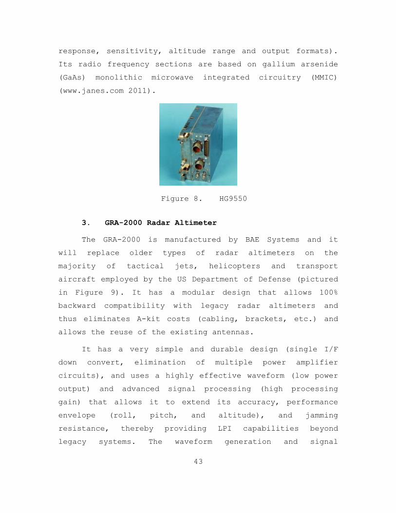
43

response, sensitivity, altitude range and output formats).

Its radio frequency sections are based on gallium arsenide

(GaAs) monolithic microwave integrated circuitry (MMIC)

(www.janes.com 2011).

Figure 8. HG9550

3. GRA-2000 Radar Altimeter

The GRA-2000 is manufactured by BAE Systems and it

will replace older types of radar altimeters on the

majority of tactical jets, helicopters and transport

aircraft employed by the US Department of Defense (pictured

in Figure 9). It has a modular design that allows 100%

backward compatibility with legacy radar altimeters and

thus eliminates A-kit costs (cabling, brackets, etc.) and

allows the reuse of the existing antennas.

It has a very simple and durable design (single I/F

down convert, elimination of multiple power amplifier

circuits), and uses a highly effective waveform (low power

output) and advanced signal processing (high processing

gain) that allows it to extend its accuracy, performance

envelope (roll, pitch, and altitude), and jamming

resistance, thereby providing LPI capabilities beyond

legacy systems. The waveform generation and signal

44

processing are all software controlled, allowing for

customization (www.janes.com 2010).

Figure 9. GRA-2000

4. PA-5429 Radar Altimeter

The PA-5429 is manufactured by the South African

company Tellumat. It is a pulsed airborne radar altimeter

that provides altitude above ground level (AGL) for heights

from 0 to 5,000 ft. It operates in the mid-J-band (~15 GHz)

and provides both analogue and discrete interfaces. It

incorporates LPI and comprehensive anti-jamming features

(www.janes.com 2007).

5. CMRA – Cruise Missile Radar Altimeter

The CMRA is manufactured by Honeywell and was

developed specifically for cruise missile programs,

including the Air Launched Cruise Missile (ALCM) and

Tomahawk missiles. It is a derivative product in which a

variety of features from other Honeywell altimeters are

incorporated. The system has the capability to perform

terrain correlation and navigation functions (www.janes.com

1994).

45

6. AHV-2XX0 Family of Radar Altimeters

These altimeters are manufactured by Thales

Communications and are designed to meet the latest

helicopter/transport aircraft (AHV-2100), fighter aircraft

(AHV-2930) and missiles/UAV (AHV-2500) requirements. They

use an improved FMCW technique that provides enhanced

accuracy, integrity, immunity to multipath, and reduced

power consumption. LPI is achieved through power management

of the RF output. The combination of a narrow receiver

bandwidth with high-performance digital signal processing

provides resistance to jamming (www.janes.com 2010,

www.thalesgroup.com 2011). A picture of the AHV-2XX0 family

of radar altimeters is presented in Figure 10.

Figure 10. AHV-2XX0 Family of Radar Altimeters

7. AD-1990 Radar Altimeter

The AD-1990, manufactured by Selex Galileo, is a

covert radar altimeter, designed to meet the UK Royal Air

Force's (RAF) needs in the 1990s. It was a form fit and

function replacement for the original altimeter of the RAF

Tornado aircraft. Its digital signal processing techniques

allow the simultaneous tracking of height, both above the

ground and above obstacles such as trees. Its covert

operation (LPI) is achieved by spreading the transmitted

signal over a very wide bandwidth through the application

46

of pseudo-random phase modulation and adaptive power

tailoring (power management) which in addition gives a high

resistance to jamming. It provides both analogue and

digital outputs (www.janes.com 2010).

8. AN/APS-147 Radar

Telephonics Corporation’s The AN/APS-147 is a maritime

Inverse Synthetic Aperture Radar (ISAR) that equips the

U.S. Navy's (USN) MH-60R multi-mission helicopter. It uses

high-throughput signal and data processing and is fully

programmable. It uses a collection of waveforms and has a

very low output power compared to traditional maritime

surveillance radars. The latter, combined with frequency

agility, provides significant LPI characteristics to this

radar. Some of its important features are the flexible

modular design, production of high-resolution images, low

input power, simple design that provides high reliability

and maintainability and a fully programmable signal

processor with multiple waveform exciter and high-

throughput rates (www.janes.com 2010). The AN/APS-147 radar

onboard a MH-60R helicopter is seen in Figure 11.

Figure 11. AN/APS-147 Radar (Antenna Under Helicopter Cockpit--Red Arrow)

47

9. AN/APQ-181 Radar

The AN/APQ-181 is manufactured by Raytheon Space and

Airborne Systems. It is a multi-mode radar for the B-2

bomber. It operates in the Ku-band (12.5 to 18 GHz) and was

designed for LPI functionality that complements the stealth

character of the B-2 bomber. Various individually effective

design and operating techniques are used in this radar

that, when integrated together, greatly diminishes the

effectiveness of enemy intercept receivers. The radar has

in total 21 operating modes, amongst them precision

position and velocity update measurement, altitude

measurement, radar-generated imagery, synthetic aperture

radar (SAR) mode and production of topographic map-like

high-quality images. All the previous modes contribute to

the achievement of a high-accuracy inertial navigation,

which permits its autonomous navigation without the aid of

GPS or other external navigation aids as well as the

precise location and identification of assigned targets. It

has two antennas, located on the left and right below the

leading edge of the platform's wing/body at 2.4 m outboard

of the aircraft center line, that are electronically

steered in two dimensions and feature a monopulse feed

design to facilitate fractional beamwidth angular

resolution (www.janes.com 2010).

10. AN/APG-77 Radar

The AN/APG-77 is manufactured by Northrop Grumman

Electronic Systems and Raytheon Space and Airborne Systems

for the F-22 fighter aircraft. It is an X-band (8 to 12.5

GHz) multimode Active Electronically Scanned Array (AESA)

48

radar. Its low observability AESA antenna has approximately

2,000 transceiver modules that incorporate MMIC technology

and also provide a low radar RCS. It is advertised to offer

long-range, multi-target, all-weather, stealth vehicle

detection, electronic intelligence gathering and multiple

missile engagement capabilities. It provides all aspect

air-to-air, dogfight and air-to-surface operating modes

that are also effective in a heavy clutter environment.

Unconfirmed sources suggest that it has an operating range

of 193 km. It has a very high bandwidth when operating in

intelligence gathering mode (approximately 2 GHz bandwidth

when it is functioning in a forward-looking, high-gain,

passive listening mode). It offers Ultra High-Resolution

(UHR) modes that are claimed to have a 31 cm resolution at

ranges in excess of 161 km (www.janes.com 2011).A picture

of the AN/APG-77 radar antenna is given in Figure 12.

Figure 12. AN/APG-77 Radar Antenna

11. LANTIRN (Low-Altitude Navigation and Targeting Infra-Red for Night)

The LANTIRN system is manufactured by Lockheed Martin

Missiles & Fire Control. It is used by F-16 and F-15E

fighter aircraft. It is a ground attack integrated system

49

that has two pods: the AN/AAQ-13 navigation pod and the

AN/AAQ-14 targeting pod. The AN/AAQ-13 navigation pod

contains a wide FoV (Field of View) FLIR (Forward Looking

Infra-Red), and the AN/APN-237 Ku-band (12.5 to 18 GHz)

terrain-following radar from Raytheon. The FLIR uses a

single MCT (mercury cadmium telluride) array and the

picture is displayed to the pilot on a wide FoV holographic

HUD. This provides the pilot with night vision for safe

flight at low level. The terrain-following radar enables

the pilot to operate at very low altitudes. It uses

advanced signal processing to provide wide azimuth

coverage, which in turn allows more violent maneuvering of

the aircraft. This is because the system can provide

directional inputs to the pilot or the flight control

computer, whereas older systems only provided pitch-up

commands. The terrain following radar can be linked

directly to the aircraft's autopilot to automatically

maintain a preset altitude down to 100 feet while flying

over virtually any kind of terrain. It has five modes:

Normal, Weather, ECCM, LPI, and Very Low Clearance (VLC).

Pictures of the LANTIRN pod aboard and F-16 fighter

aircraft and the AN/AAQ-13 navigation pod, respectively,

are given in Figures 13 and 14.

50

Figure 13. LANTIRN Pods on F-16--Red Arrows

Figure 14. AN/AAQ-13 Navigation Pod

12. RBS-15 Mk3 Missile Seeker

The RBS-15 is manufactured by Saab Dynamics AB. It is

a medium range radar guided anti-ship/land-attack missile.

The RBS-15 Mk2’s radar seeker uses FMCW technology and has

a very low power output (in the mWatt range) (Pace 2009,

59). The broadband, frequency-agile radar with its digital

processing is claimed to provide a high ECCM performance.

The RBS-15 Mk3 missiles have an improved monopulse high Ku-

band (35 GHz) radar seeker (www.janes.com 2010). Further

developments (already tested) of the seeker are the

introduction of an LPI radar using FMCW wave spread-

51

spectrum technology, improvements of the angular resolution

and target discrimination of the seeker through synthetic

aperture radar (SAR) techniques, as well as studies to

integrate the seeker with an imaging infra-red (IIR) sensor

(www.janes.com 2011).

B. MARITIME LPI RADARS

1. Pilot Radar

The Pilot is manufactured by Saab Bofors Dynamics. It

is an X-band (8 to 12.5 GHz) LPI navigation and threat

detection radar. It uses the FMCW transmission technique

and it is suitable for coast guard vessels, fast attack

craft, fast patrol boats, frigates, submarines and

coastal/land surveillance applications. It can function

both in stand-alone and add-on configurations. In the add-

on configuration the Pilot radar uses the X-band antenna of

the platform’s existing radar, which can be any available

pulsed navigation radar system. The aforementioned

capability uses a wave-guide switch that allows either the

Pilot or the conventional radar's transceiver to use the

antenna as required. Other important features of the Pilot

radar are the low average power output, the 2.4 m range

cell resolution, the resistance to electronic support

system detection and/or anti-radiation missile attack, and

the use of a “fully” solid-state transceiver(www.janes.com

2010).A picture of the Pilot radar onboard a Visby-class

corvette is given in Figure 15.

52

Figure 15. Pilot Radar on Visby-class Corvette (Radar Antenna--Red Arrow)

2. Scout Radar

The Scout is manufactured by Thales Netherlands. It is

an I-band (8 to 10 GHz) LPI surface surveillance and

tactical navigation radar, and is an improved version of

the Pilot radar. This improvement has to do mainly with the

FMCW transmission technique used by the Scout radar. It

incorporates a dual array antenna that features optimal

isolation between transmit and receive elements in order to

maximize range performance. It can function both in stand-

alone and add-on configurations. In the add-on

configuration, an I-band pulse radar uses the Scout dual

array antenna (with the addition of a waveguide and

waveguide switch) for both pulsed and FMCW functionality.

Other important features of the Scout radar are the low

average power output (10mW to 1 W selectable by the user),

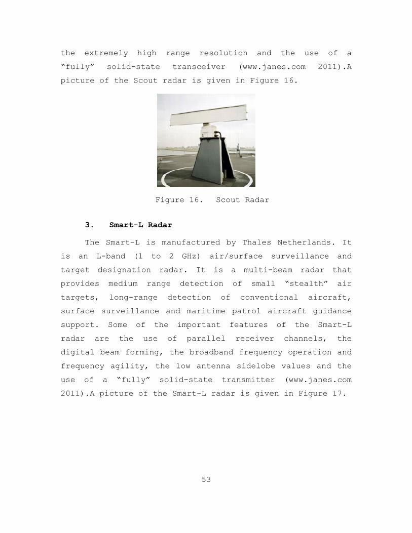
53

the extremely high range resolution and the use of a

“fully” solid-state transceiver (www.janes.com 2011).A

picture of the Scout radar is given in Figure 16.

Figure 16. Scout Radar

3. Smart-L Radar

The Smart-L is manufactured by Thales Netherlands. It

is an L-band (1 to 2 GHz) air/surface surveillance and

target designation radar. It is a multi-beam radar that

provides medium range detection of small “stealth” air

targets, long-range detection of conventional aircraft,

surface surveillance and maritime patrol aircraft guidance

support. Some of the important features of the Smart-L

radar are the use of parallel receiver channels, the

digital beam forming, the broadband frequency operation and

frequency agility, the low antenna sidelobe values and the

use of a “fully” solid-state transmitter (www.janes.com

2011).A picture of the Smart-L radar is given in Figure 17.

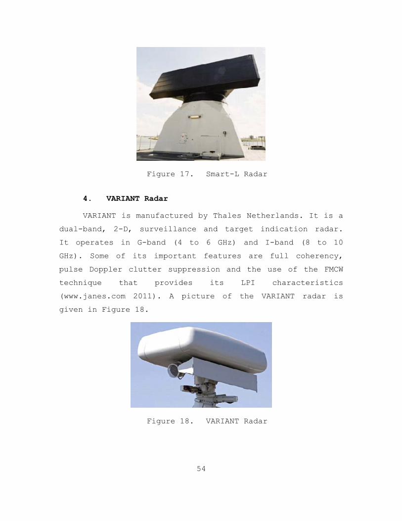
54

Figure 17. Smart-L Radar

4. VARIANT Radar

VARIANT is manufactured by Thales Netherlands. It is a

dual-band, 2-D, surveillance and target indication radar.

It operates in G-band (4 to 6 GHz) and I-band (8 to 10

GHz). Some of its important features are full coherency,

pulse Doppler clutter suppression and the use of the FMCW

technique that provides its LPI characteristics

(www.janes.com 2011). A picture of the VARIANT radar is

given in Figure 18.

Figure 18. VARIANT Radar

55

5. AN/SPN-46 (V) Precision Approach Landing System

The AN/SPN-46(V) is manufactured by Textron Defense

Systems. It is a precision approach landing system that

provides simultaneous and automatic control for up to two

aircraft during final approach and landing aboard aircraft

carriers and other landing platforms. The heart of the

system is a precision dual-band automatic

acquisition/tracking radar that features cross-band beacon

and aircraft skin tracking. It operates in X-band (8 to

12.5 GHz) and K-band (20 to 40 GHz) (www.janes.com 2010). A

picture of the AN/SPN-46 radar is given in Figure 19.

Figure 19. AN/SPN-46 (V)3

C. LAND-BASED LPI RADARS

1. TALS--Tactical Automatic Landing System

The TALS is manufactured by Sierra Nevada Corporation.

It is an Automatic Unmanned Aerial Vehicle (UAV)

recovery/tactical automatic landing system that provides a

day/night, all weather, automatic landing and take-off

capability for UAVs operating in tactical or fixed-base

land environments. It operates in K-band (35 GHz ±150 MHz)

3www.navair.navy.mil 2011

56

and it has a wide bandwidth (up to 20 MHz), which gives the

radar its LPI characteristics (www.janes.com 2011). A

picture of the TALS is given in Figure 20.

Figure 20. TALS

2. Eagle Fire Control Radar

The Eagle is manufactured by Saab Group. It is a

“silent” millimetric system that is used in mobile ground

and naval-based air defense applications. It operates

within the K-band (35 GHz center frequency) and is

optimized for low altitude target tracking. Its LPI

characteristics come from the fact that it uses pulse

compression, a high gain antenna with low sidelobe values,

and a low output peak power figure. The manufacturer claims

that its antenna radiation pattern, in combination with its

transmission technique, makes it impossible for

escort/standoff jammers to degrade its performance. It also

incorporates an operating mode that allows simultaneous

pulse-to-pulse frequency agility and Moving Target

57

Indication (MTI) (www.janes.com 2010). The Eagle fire

control radar is seen in Figure 21.

Figure 21. Eagle Fire Control Radar

3. HARD-3D Radar

The HARD-3D is manufactured by Saab Group. It is an

all-solid-state 3D-search-and-acquisition radar designed

for use in short-range air defense systems such as the

Atlas Short Range Air Defense (ASRAD). The electronically

scanned beam in elevation achieves the 3D capability of the

radar. Its LPI characteristics are due to its very low

electromagnetic signature, (low output peak power 240 W,

low average power 30 W), its broadband frequency agility,

the low sidelobes and the narrow antenna beam

(www.janes.com 2011). The HARD-3D radar is seen in Figure

22.

58

Figure 22. HARD-3D Radar

4. POINTER Radar

The POINTER is manufactured by Ericsson Microwave

Systems. It is an LPI all-solid-state 3D radar that

operates in X-band and has been designed to integrate into

short-range air defense missile systems such as the

Mistral, Stinger and Starburst. The technology implemented

on the Pointer radar came from the developer’s experience

with Eagle and HARD-3D radars. The Pointer radar is a

further development of the HARD-3D radar (www.janes.com

2005). The Pointer radar is seen in Figure 23.

Figure 23. Pointer Radar

59

5. PAGE Radar

The Portable Air defense Guard Equipment (PAGE) is

manufactured by Thales Netherlands. It is a man-

portable/vehicle-mounted J-band (10-20 GHz) low-level air

surveillance radar designed for use in very short-range air

defense applications involving both anti-aircraft guns and

man-portable air defense equipment. It uses the FMCW

technique, which in combination with its very low power

output (20 W) can make the system “nearly undetectable” by

electronic support and radar warning receivers

(www.janes.com 2011). The PAGE radar is seen in Figure 24.

Figure 24. PAGE Radar

6. CRM-100 Radar

The CRM-100 is manufactured by Przemyslowy Instytut

Telecomunikacji (PIT), Poland. It is a “quiet,” LPI, solid-

state, FMCW radar designed to detect and track up to 40 sea

surface targets and automatically handoff data to a command

system. Some of its applications are monitoring of “sea

borders” for “fraud” traffic and illegal immigrants,

monitoring of economic interest zones, and search and

rescue. It operates in X-band (8-12.5 GHz) and its transmit

60

power is very low (1mW – 1W). Its LPI characteristics are

due to the FMCW technique and the power management

(www.janes.com 2011). The CRM-100 radar is seen in Figure

25.

Figure 25. CRM-100

7. JY-17A Radar

The JY-17A is manufactured by ECRIEE, China. It is a

battlefield surveillance radar that operates in X-band (8-

12.5 GHz). It is a fully coherent, solid-state sensor

suitable for ground or vehicle based applications. It is

designed to detect, localize and identify moving targets on

the battlefield (including low-flying air vehicles) in

“severe” electronic countermeasures and clutter

61

environments. Specific role applications include

battlefield surveillance, artillery fire adjustment, border

surveillance and high-value asset protection. Its main

features are the modular design, the LPI functionality, its

solid-state transmitter, digital pulse compression, pulse-

Doppler filter bank processing and automatic target

detection and tracking (www.janes.com 2004).

62

THIS PAGE INTENTIONALLY LEFT BLANK

63

IV. DETECTION OF LPI RADARS

As discussed in Chapter II, one of the main

characteristics of the LPI technology is its wideband

nature. The concept behind utilizing wideband techniques is

to spread the radiated power over a large bandwidth, in

order to produce a Power Spectral Density (PSD) below the

noise level of the receiver. By reducing the input power at

the receiver, signal detection relies on extending the

integration time period, during which a special integration

procedure must be applied to exclude noise being added in

the same amount (Burgos-Garcia, et al. 2000).

Another point of concern for the receiver is the

element of sensitivity, as the detection of the wideband

LPI signal has to take place against a background saturated

with short duration, conventional radar signals in the same

band (Denk 2006). Without neglecting the centrality of the

sensitivity factor, the performance trends in radar warning

receivers are primarily improvements to obtain higher

dynamic range and higher frequency resolution, not in the

direction of improved sensitivity (Lynch Jr. 2004).

Signal processing comprises another critical area of

consideration for the receiver. LPI radars can integrate

their reflected signals coherently over the whole of the

integration time, thus narrowing the receiver noise

bandwidth and increasing sensitivity. On the other hand, ES

receivers cannot coherently detect the radar’s signals and

hence they cannot narrow their bandwidths in the same

manner (Fuller 1990). In most cases today, the signal

processor in an intercept receiver is considerably less

64

powerful than its counterpart in radars or data links.

Based on netted situational awareness, modern processors

will also be dynamically programmed to threat frequency

bands (see Chapter V).

The increased sophistication of modern radar systems

results in an electro-magnetic environment where the

receiver should expect very few pulses. Staggered PRF and

frequency agility techniques, which can be implemented by

track-while-scan or LPI radar, further complicate the issue

of identification. This is especially true for LPI CW

radars and digital pulsed radars that utilize an enormous

number of complex modulations; as these modulations can

result in many reports for a single diverse emitter, they

render accurate identification more difficult (Pace 2009).

The situation is exacerbated in the presence of ultra-

wideband sources such as spread spectrum communication

signals, impulse radars and impulse jammers. Sources such

as ultra wideband SAR and ISAR imaging radar, whether

intercepted intentionally or not, can significantly raise

the noise floor of the receiver, disabling the ability of

the EW receiver to detect the important threats of interest

(Pace 2009). In addition, the EW receiver must have high

power detection and protection circuits at the front end to

protect itself from deliberate destruction by directed

energy weapons.

Reaction time is another crucial challenge for LPI

detectors, especially in the face of modern range Doppler

imaging missiles: employing sophisticated FMCW modes to

improve target aiming accuracy and reject eventual decoys,

65

power managed seekers adjust the transmitter power in such

a manner that the received power at the EW receiver is kept

constant.

All aforementioned concerns have been quantified into

seven generic factors that need to be taken into account

for the LPI radar signals to be detected by Electronic

Warfare Support (ES) receivers (Lynch Jr. 2004):

1. LPI system mainlobe power at the intercept receiver

2. LPI system sidelobe power level at the intercept

receiver

3. Area of mainlobe and sidelobes on the ground or at

a certain threat altitude

4. Time of Area of Regard (AOR) illumination for

mapping, tracking, or targeting

5. Intercept receiver density and search time

6. Intercept receiver detection response

7. Power management strategy

The vital task of detection is followed by

classification, a process that requires sorting the signal

into groups having similar parameters that distinguish one

LPI radar signal from another:

• LPI radar type

• Carrier frequency

• Modulation bandwidth

• Modulation period

• Code period

66

• Time and angle of arrival.

Subsequent correlation with an electronic emission

library (database) can then aid in signal tracking and

response management (identification). This process,

commonly known as Specific Emitter Identification (SEI),

attempts to fingerprint the emitters that are intercepted.

Several algorithms have been investigated for doing SEI but

their details remain classified (Pace 2009, 402). The

research conducted for this thesis indicates that Fourier

analysis remains the fundamental tool. Commencing from this

basic tool, more complex signal processing techniques have

evolved, such as the Short Time Fourier Transform (STFT),

which aims at tracking signal parameters over time. More

sophisticated techniques have also been developed, called

time-frequency and bi-frequency distributions, to identify

the different modulation schemes used by the LPI radar

(e.g., Wigner Ville Distribution (WVD) and Quadrature

Mirror Filter Bank (QMFB) [Pace 2009, 405-510]).

A. ES RECEIVER CHALLENGES

To detect LPI radar signals, ES receivers have to

overcome two major difficulties:

• Processing gain of the LPI radar

• High sensitivity requirement

1. Radar Processing Gain

In the second chapter of this thesis, range factor α

was defined as Iα R= . Assuming IR to be the detection range

of the interceptor and rR the detection range of the radar,

range factor can be defined as:

67

4.1I

R

Rα R=

If 1α > , the radar will be detected by the intercept

receiver platform. If 1α ≤ , the radar can detect the

platform while the intercept receiver platform cannot

detect the radar.

When the same radar antenna is used to both transmit

and receive ( Tx RxG G≈ ) and an omnidirectional intercept

antenna ( 1G = ) is used for the interceptor, then a certain

energy or average power transmitted range factor α can be expressed directly in terms of the radar waveform, antenna

pattern and radar cross section as:

41 1 4.2I Ti

R Tγ i

R Gα KR RG τB σ= = ⋅ ⋅

where K is the constant parameter of the equation, TiG is

the antenna gain in the direction of the interceptor, iB is

the equivalent noise bandwidth of the intercept receiver, τ is the integration time of the LPI radar, and σ is the radar

cross section of the target. This equation indicates that

the value of α is directly proportional to the square root of the radar antenna gain in the direction of the

interceptor, to the fourth root of the radar cross section

and inversely proportional to the time-bandwidth factor

( iτB ), which also comprises the processing gain of the radar

receiver over the intercept receiver (Lee 1991, 55).

68

2. High Sensitivity Requirement

Some ES receivers do not have sufficient sensitivity

for the detection of LPI radar signals. Jim P. Lee states

that for an over-the-horizon operation (OTHT), system

sensitivity should be no less than -100dBmi. Accounting for

the pre- and post-detection bandwidth of the receiver, Lee

provides a formula different than the one provided in

Chapter II (Equation [2.6]) for the calculation of

sensitivity:

( )1Ι 1 22 4.3γγI i iδ n SNR G B B −

=

Where:

in : Receiver noise power density

iSNR : The threshold signal-to-noise ratio

iG : Intercept receiver antenna gain

1B : Pre-detection bandwidth

2B : Post-detection bandwidth, and

γ : Α parameter ranging between 0 0.5γ< < .(Lee 1991, 55)

In Equation (4.3), the pre-detection bandwidth 1B

defines the instantaneous bandwidth of the intercept

receiver over which it can detect signals. The post-

detection bandwidth 2B defines the maximum modulation rate

that the intercept receiver can measure. The parameter γ determines the effective bandwidth of the receiver and

69

varies from a value of 0.5 when 1 2B B< , (characteristic of a

wide-open, high probability of intercept receiver), to a

value of 0 when the two bandwidths are comparable

(characteristic of a high sensitivity search receiver).

A careful examination of Equation (4.3) reveals that

the ES receiver has three basic means for increasing its

sensitivity: increasing the antenna gain, reducing the pre-

detection bandwidth, and reducing the post-detection

bandwidth. In order to improve sensitivity further, both

the noise figure and transmission loss of the ES receiver

should be minimized.

The first two means involve a probability of intercept

(POI) loss by reducing either the angular or frequency

instantaneous coverage. The third merely represents a

reduction in the measurement bandwidth of the intercept

receiver. Therefore, for operation against high duty cycle

LPI waveforms, there is scope within conventional ES

receivers for increasing sensitivity at negligible cost by

reducing the post-detection bandwidth without compromising

the POI (Ruffe and Stott 1992, 200-202).

B. TYPES OF ES RECEIVERS FOR LPI RADAR DETECTION

There are six general kinds of intercept receiver

implementation (see Table 5). The first and simplest class

is wideband channelized Crystal Video Receivers (CVRs) with

RF preamplifiers. The second class, which is widely used,

is Instantaneous Frequency Measuring (IFM), usually

employing preamplifiers and wideband channelization. The

third class is digitally controlled scanning

superheterodyne/homodyne receivers, which are characterized

70

by narrowband filters that are swept over the frequency

range of interest. Fourth are completely channelized high-

dynamic-range intercept receivers that are characterized by

wide frequency coverage but broken into reasonably small

filter bins, implemented with multiple discrete filters to

provide very high dynamic range. Fifth are transform

receivers (microscan, Bragg cell, or compressive), which in

essence form a filter bank from a frequency-dispersive or

optical device. Sixth and last are hybrids of the above

types, which allow cueing of high-resolution, high-dynamic-

range analysis receivers.

Table 5. Intercept Receiver Typical Performance4

The performance trends in radar warning receivers are

primarily improvements to obtain higher dynamic range and

higher frequency resolution, not in the direction of

improved sensitivity.5 Research indicates that the usable

sensitivity is always limited by the environment and not by

Boltzmann’s constant (Lynch Jr. 2004). The second area

where improvements will occur is signal processing. In most

cases today, the signal processor in an intercept receiver

4Lynch Jr., 117. 5For an argument in favor of improved sensitivity, see: Aytug Denk,

Detection and Jamming Low Probability of Intercept (LPI) Radars, Master's Thesis, Electronic Warfare, Naval Postgraduate School (NPS) (Monterey: NPS, 2006).

Parameter/Type CVR IFM Superhet. Channelized Transform Cueing Instantaneous

Bandwidth Excellent Poor Poor Good Good Excellent

Simultaneous signals Poor Excellent Poor Good Good

Frequency Resolution Poor Good Excellent Good Good Excellent

Dynamic Range Good Fair Excellent Very Good Fair Excellent Usable

Sensitivity Poor Fair Excellent Good Fair Excellent

71

is considerably less powerful than its counterpart in

radars or data links. Processors also will be dynamically

programmed to treat frequency bands based on netted

situational awareness. The rate of the developments in

signal processing is so great relative to the rest of the

technology that dramatic improvements in signal processing

can be expected over the coming decades. What this will

require of stealth systems is spreading the emissions over

wider and wider operating bands and creating more complex

operating and spoofing waveforms.

1. Crystal Video Receiver

CVRs are the most common types of intercept receivers,

one of their most common commercial uses being radar

automobile speed trap detectors. In fact, the simplest

ELINT system is the crystal video type consisting of an

antenna, a detector, and a video amplifier (Wiley, ELINT:

The Interception and Analysis of Radar Signals 2006, 57-

63). A typical CVR block diagram is provided in Figure 26.

Figure 26. CVR Block Diagram

72

It consists of one or several omni-directional

antennas, which are frequency multiplexed into a small

number of RF amplifier channels. (CVRs have broad

channelization, e.g., X, Ku, IR, and UV). Subsequent to

this channelization, which typically might be 1 GHz in

bandwidth, the output is detected and compressed in a log

compressive video amplifier. The amplitude-compressed

outputs in each of the bands are then processed with

respect to pulse train shape, angle of arrival, and general

frequency of operation.

In their simplest form, CVRs have too much sensitivity

and create many false alarms unless thresholds are set very

high (–35 to 40 dBm). Extra sensitivity can be provided

with the use of an additional low-noise RF preamplifier:

from a level of –35 to –55 dBm without a preamp, an RF

preamplifier may increase its sensitivity down to –85 dBm.

The tangential sensitivity of a CVR is:

( )2

26.31 2.5 2 4.4νν RF ν ν

ABTSS kTF B B B BGF

⎛ ⎞⎜ ⎟= + − +⎜ ⎟⎜ ⎟⎝ ⎠

Where:

k : Boltzmann’s constant ( 231.38 10 W/K−⋅ )

T : Room temperature (290K )

F : Noise figure of amplifiers ahead of detector

νB : Video bandwidth (Hz)

RFB : RF bandwidth (Hz)

73

A : Diode parameter

G : Gain of the amplifiers ahead of the detector

The diode parameter is given by the formula:

24 4.5

νF RA kTC=

Where

R : Dynamic impedance of the detector (Ω)

C : Detector sensitivity (V/W)

CVRs are very mismatched in the optimal detection

sense, but they were designed for high peak power and short

ranges, for which they are quite adequate. The crystal

video receiver is characterized by broad instantaneous

bandwidth and low sensitivity. Front-end bandwidths are

typically 200 MHz up to 4 GHz.

The advantages of such a system are that the design is

simple by military standards, relatively inexpensive, not

spoofed by complex waveforms, and in a low-density signal

environment, every bit as good as the more elaborate

receivers. The principal disadvantage is lack of

selectivity, which is a severe problem in dense signal

environments. Its sorting capability is limited, because

frequency resolution and angle of arrival accuracy is

usually poor. In addition, sensitivity is usually limited

by RF preamplifier bandwidth. The sensitivity limitation,

however, is usually not significant, because the poor

74

selectivity prevents the handling of very many signals so

that noise limited thresholds can never be approached.

2. Instantaneous Frequency Management Receivers (IFM)

A leading member of the channelized receiver family,

IFMs were developed in response to the need to measure the

frequency on each pulse. IFMs are essentially a CVR with

the addition of a frequency sensing method, usually

dividing the signal into two paths with a short delay

inserted in one of them. The IFM receiver principal can be

understood from Figure 27. The frequency measuring

reference in this scheme is a delay line, which results in

the channelizing of the frequency spectrum to an accuracy

that is on the order of the reciprocal of the delay line

time length.

Figure 27. IFM Principle

75

Indeed, by comparing the phase of the signals, the

phase shift ends proportional to the carrier frequency:

2 4.6θ πfτ=

Where:

θ : Phase shift (radians)

f : Carrier frequency (Hz) τ : Differential delay (sec)

As the frequency is proportional to the phase

difference, for a given delay, the unambiguous band covered

is that for which the phase-change is 1/τ (Wiley, ELINT: The Interception and Analysis of Radar Signals 2006, 74).

Intensity is usually thresholded to control noise. The

signal above that threshold is usually log compressed by a

pre-emphasis circuit so that there is a correspondence with

a range reticle on the display. Modern digital IFMs have

multiple delay lines with binary ratios and thresholded

outputs that are encoded into a frequency tag word as shown

in Figure 28.

76

Figure 28. Digital Multioctave IFM Block Diagram

The major advantages of an IFM are its good frequency

accuracy and moderate to good sorting capability in an

interference-free or low-signal-density environment. In

addition, IFMs are not confused by wide-bandwidth

modulations such as chirp and frequency hopping. With a

low-noise preamp, sensitivities can reach a level of –85

dBm. In general, however, performance is not degraded by

noise, but by signal density and processing capacity.

The major disadvantage of the IFM receiver is its

complexity, which unavoidably renders it more expensive

than CVRs. The absence of a high dynamic range frequency

preselection ahead of the IFM renders it vulnerable to

overlapping or pulse-on-pulse signal environments. Usually,

in the presence of overlapping pulses, dynamic ranges are

never greater than 25 dB, and the more overlapping pulses,

the greater the number of false targets (Lynch Jr. 2004,

123).

77

The IFM is generally a good compromise between

channelized and crystal video intercept receivers for many

applications.

3. Superheterodyne Receiver

This type of receiver is the most widely used design

in nearly all applications. It uses a local oscillator to

convert the incoming signal to a fixed intermediate

frequency (IF). After this mixing process (heterodyning),

the IF amplifier need operate at only one frequency and its

characteristics can be precisely controlled (bandwidth,

center frequency, gain, band edge roll-off, group delay).

One of the most common channelization schemes used today is

the digitally controlled scanning superheterodyne design

(Figure 29).

Figure 29. Digitally Controlled Superheterodyne Receiver Block Diagram

The scanning superheterodyne receiver in Figure 31

consists of a swept preselection filter: e.g., swept YIG

resonator, a swept local oscillator, a narrowband

intermediate frequency filter detector, a logarithmic

amplitude compressor, and a signal encoder. All subunits

are digitally controlled by computer as to frequency, sweep

rate, and threshold by a threat table. The effects of

78

harmonic distortion are reduced with the use of a pre-

selection filter, the bandwidth of which is determined by

the local oscillator harmonic spacing; the higher the local

oscillator frequency, the wider the preselector bandwidth

can be. The controlled frequency synthesizer successively

locates the narrowband IF filter-detector across the band

of interest by means of the mixer output signal (usually

the first difference term). The bandwidth of the IF filter

is selected to be approximately matched to the narrowest

pulse to be detected. Subsequent to filtering, the pulses

are detected and amplitude compressed. Amplitude

compression is required to compress the typical 1012dynamic

range down to even 100:1 (Wiley, ELINT: The Interception

and Analysis of Radar Signals 2006, 125). The encoder

output usually includes the pulse amplitude, pulse width,

time of arrival, frequency, and special parameters, i.e.,

CW or FM waveforms.

The scanning superhet has a single or small number of

narrowband filters whose frequency locations are swept

according to some pre-programmed strategy. The tradeoff for

their improved noise performance—due to their narrowband

nature—is a large mismatch with respect to the intercepted

signal. Usually, the sweep rate is low in dense threat

bands and high in bands in which there are few threats.

The dynamic range for superhets is extremely high and

is often limited by the threat table to a value related to

lethal range. For example, the threshold for the AN/ALR-56M

Radar Warning Receiver (RWR) is programmed by frequency

band based on the threat effective engagement range that

reduces pulse traffic in the receiver.

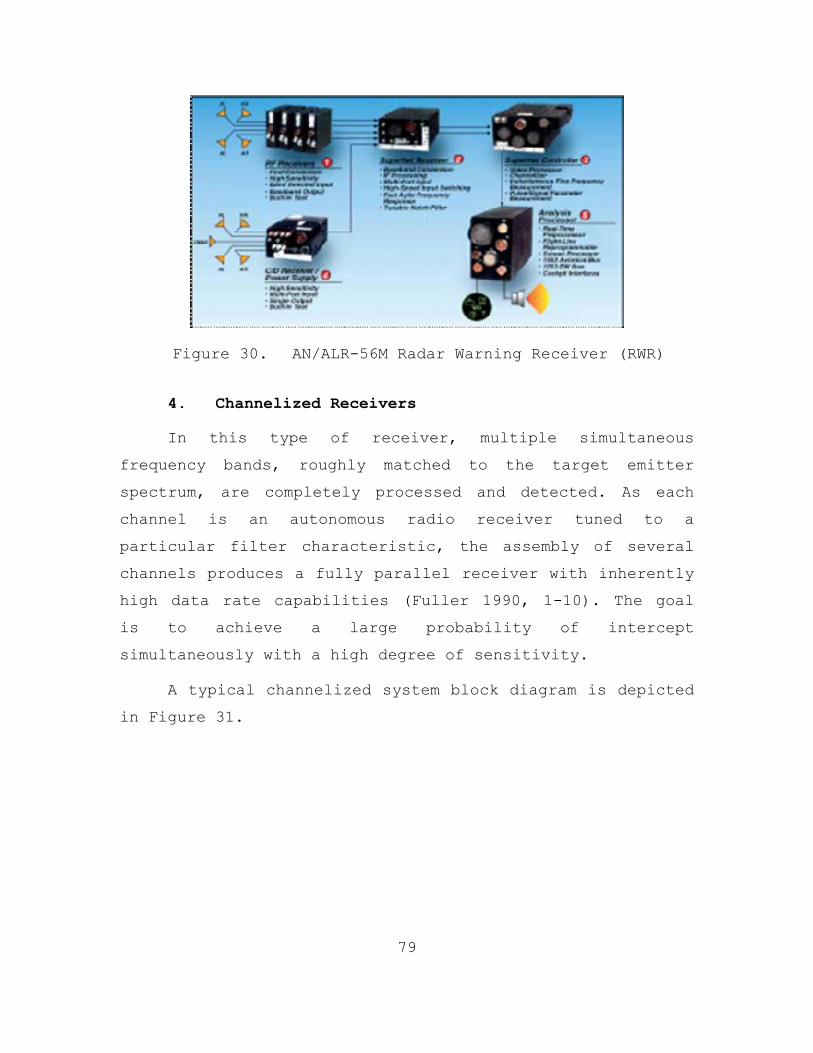
79

Figure 30. AN/ALR-56M Radar Warning Receiver (RWR)

4. Channelized Receivers

In this type of receiver, multiple simultaneous

frequency bands, roughly matched to the target emitter

spectrum, are completely processed and detected. As each

channel is an autonomous radio receiver tuned to a

particular filter characteristic, the assembly of several

channels produces a fully parallel receiver with inherently

high data rate capabilities (Fuller 1990, 1-10). The goal

is to achieve a large probability of intercept

simultaneously with a high degree of sensitivity.

A typical channelized system block diagram is depicted

in Figure 31.

80

Figure 31. Channelized Intercept Receiver Block Diagram

It consists of an antenna or set of antennas,

multiplexers, and filters. RF channels are frequency

multiplexed to an intermediate frequency where multiple

local oscillators place 50 to 200 MHz segments of the

received band into narrow filters. The outputs of these

individual filters are down-converted again, folded in

frequency by re-sampling to save hardware, detected, and

video filtered. Those sampled outputs are encoded in

amplitude, phase, pulse width, and so on (Lynch Jr. 2004,

126).

A channelized receiver’s major advantage is that

sensitivity is usually limited only by thermal noise,

because sorting problems are minimized. In addition,

channelized receivers have excellent frequency resolution,

which not only provides good sorting capability but also

minimizes interference in a dense signal environment.

Finally, the reduced processing load allows dramatically

improved usable sensitivity and much better emitter

classification (Lynch Jr. 2004, 128).

81

The disadvantages of such systems occur primarily in

issues of complexity and cost. Other limitations have to do

with the spectral purity of the multiplicity of local

oscillators and signal ambiguity in a dense emitter

environment caused by folding. The narrow bandwidth may

also result in some desensitization or false targets when

chirp, frequency-hopping, or phase-coded signals are

utilized by the target emitters.

5. Transform Intercept Receivers

This type of receiver approximates a Fourier

transform. Among the most common ways of implementing them,

are compressive devices such as Brag cells and microscans,

designed to operate at scan times on the order of the pulse

lengths from the target emitter class. The microscan

compressive receiver—practically a channelized receiver—

suffers the same inherent disadvantages as an IFM receiver:

limitation in instantaneous dynamic range. As David Lynch

notes, instantaneous dynamic range limitations can be a

source of serious implications in dense emitter

environment. Another inherent shortfall, inevitable due to

the non-linearities that exist in all receivers, has to do

with harmonic distortion caused by simultaneously received

multiple signals. This distortion ends in signal

misclassification in frequency, direction, amplitude,

number of pulses present, and so on. An additional side

effect of nonlinearities is small signal suppression;

consequently, in an environment in which LPI systems co-

exist with conventional systems, the conventional emitter

may completely mask the LPI systems (Lynch Jr. 2004, 128).

82

6. Cueing Systems/Hybrid Systems

Cueing or hybrid systems are a combination of two or

more of the previous receiver types. Alerting, angle and

frequency estimates from the first receiver (coarse

receiver) are used to cue a second receiver with higher

resolution and dynamic range for tracking, sorting, and

classification. Adequate signal storage is provided by

wideband delay lines so that the coarse receiver can

command the high-resolution receiver to the correct

frequency band and angular quadrant for high-resolution

measurement. A typical block diagram is shown in Figure 32.

Figure 32. Hybrid Receiver Block Diagram

Hybrid receivers are capable of wide coverage while

still providing high enough resolution to simplify

processing, which allows higher sensitivity.

One major advantage of this configuration is its

higher resolution analysis band, which can separate

overlapping pulse trains and similar signals with greater

ease. This happens because the probability of many signals

83

over a narrower angle and frequency space is greatly

reduced, allowing thus higher sensitivity to be used, as a

consequence of reduced probability of processor overload.

The disadvantages of the hybrid class of receiver are

complexity, cost, and sensitivity to overload if all the

signals come from the same quadrant and frequency bands

(which they often do in wartime).

84

Parameter /Type

CVR IFM Superhet. Channelized Transform Cueing

Frequency Coverage

4-32GHz 1-18GHz 0.5-18GHz 0.2-18GHz 1-10GHz 0.2-35GHz

Bands 3 5 6 8 4 18 RF Bandwidth Octave Octave 500MHz 2GHz 1GHz 2GHz Video Bandwidth

20MHz 20MHz 10MHz 10MHz 2GHz 10MHz

Sensitivity -35 to -55dBbm -65 to -85dBbm -85dBm -85dBm -75dBm -85dBm Instantaneous dynamic range at frequency separation

45dB@ 85MHz 65dB@ 275MHz 70dB @1GHz 0dB @10MHz 50dB @30MHz 70dB @200MHz

0dB @3MHz 30dB @30MHz 50dB @300MHz

0dB @10MHz 50dB @30MHz 70dB @200MHz

Pulse traffic capacity

<100k pps <100k pps <1Mpps 1Mpps, processor limited

150Mpps, processor limited

>1Mpps, processor limited

Frequency Resolution

Octave Octave 10MHz 10MHz 3MHz 10MHz

Frequency accuracy

- 0.001 of band center

0.001 of band center

3MHz 3MHz 3MHz

Adjacentpulse recovery time

300nsec 50nsec 10μsec 200nsec 200nsec 200nsec

Coverage scan rate

1sec 1sec 1sec 1sec 0.3μsec 1sec

Advantages Simple, broad instant bandwidth, inexpensive, easy to use if sensitivity low

Good frequency resolution, god sorting capacity in low-density signal environment, handles wideband modulation

Very good sorting capability, high usable sensitivity, good in dense signal environments, very good frequency resolution

Sensitivity limited only by ambient and thermal noise, good frequency resolution, excellent sorting capacity in dense signal environment

Good frequency resolution, wide instantaneous bandwidth, good sensitivity

Best dynamic range on a small emitter subset, good in dense signal environment, good for broadband emitters

Disadvantages Limited sensitivity. Limited to low density signal environment, very limited sorting capability

Confused by overlapping pulses, more complex and expensive than CVR

Long scan times, narrow bandwidth limits, detection of wideband modulation, low probability of intercept for transient emitters

Complex, expensive, narrow bandwidth limits, detection of wideband modulation

Complex, expensive, poor dynamic range limits in dense signal environment, difficult signal processing

Complex, expensive, longer search time

Table 6. Typical ES Receivers' Performance Parameters6

6Lynch Jr., 123-169.

85

C. DETECTION ACCURACY

1. Detection Finding Techniques

The three basic ways in which emitters can be located

are triangulation (determination of two lines of bearing

from known locations to the emitter), determination of

distance and one line of bearing, and determination of two

mathematically described curves that cross the emitter’s

location (D. L. Adamy. 2004, 156). To measure the direction

of arrival (DOA) of the emitter signals in the first two

approaches, Adamy has listed five principal direction

finding (DF) techniques.

a. Rotating Directional Antenna

This technique exploits the relation between the

gain pattern of a rotating antenna and the angle from its

bore sight: knowing the pattern of the antenna’s gain, two

or more intercepts within the antenna main beam are

sufficient to determine the orientation which would place

the signal at the antenna bore sight. As the DF accuracy is

dependent on the size of the beam and consequently on the

size of the antenna, this approach is very common in naval

EW assets where the antenna size is not a major concern.

b. Multiple Antenna Amplitude Comparison

This approach utilizes the difference in

amplitude ratio between two differently oriented antennas

that both intercept the same signal. As no large antennas

are needed, it is widely used in aircraft radar warning

receivers (RWRs), yet its accuracy is typically low (50-150)

86

c. Watson Watt

This technique uses three antennas in line,

separated a quarter-wavelength apart. The sum and

difference patterns of the outside antennas generate a

cardioid vs. angle graph; switching among eventual

symmetrical pairs causes rotation of the cardioid graph,

allowing DF measurement. The Watson-Watt approach provides

moderate DOA accuracy (approximately 2.50RMS).

d. Doppler

This technique utilizes a rotating and a non-

moving antenna; the received signal frequency in the

rotating antenna follows a sinusoidal Doppler shift pattern

relative to the signal received at the non-moving antenna.

The direction of signal arrival is the angle at which the

Doppler shifts from positive to negative. Typical accuracy

for this technique is 30.

e. Interferometer

Interferometry in direction finding is based on

measuring the phase of a received signal at each of two

antennas. The emitter bearing is then computed utilizing

the phase difference between them (D. L. Adamy.2004, 162-

3).

As the biggest exploitable weakness for stealth

emitters in intercept receivers is the angle of arrival

(AOA), a weakness that also cascades into range estimation,

two major methods have been developed for its measurement:

amplitude angle of arrival and phase angle of arrival. In

both methods, there is a signal-to-noise-limited lower

bound on measurement accuracy. Assuming a matched filter in

87

the presence of white noise (best case), then the lower

bound rms error will be (Lynch Jr. 2004, 149):

3 4.7cos 2θλσ

π θ SNR≥

l

Where

l : Aperture length (m) and

θ : AOA of the intercepted signal

f. Amplitude Angle of Arrival

Due to its simplicity, amplitude comparison is

the primary method used in most RWRs where broadband

cavity-backed spiral antennas are used in each in each

quadrant. For bandwidths around 20 GHz, David Lynch

estimated that this type of antenna has the following gain

pattern.

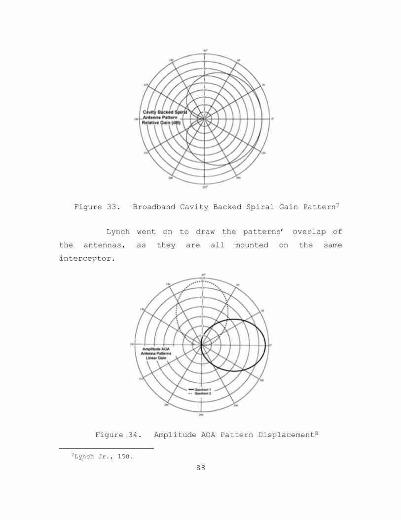
88

Figure 33. Broadband Cavity Backed Spiral Gain Pattern7

Lynch went on to draw the patterns’ overlap of

the antennas, as they are all mounted on the same

interceptor.

Figure 34. Amplitude AOA Pattern Displacement8

7Lynch Jr., 150.

89

The system structure to estimate the AOA is

fairly simple: after its filtering, each quadrant signal

passes through a logarithmic amplifier, and the difference

between any two quadrants is multiplied by an angle scale

factor and fitted to a correction curve to estimate angle

of arrival. For a set of three idealized quadrant antennas,

the angle of arrival measurement by amplitude would look as

follows.

Figure 35. Angle of Arrival Measurement by Amplitude Comparison9

Figure 35 shows three idealized quadrant antenna

patterns; it can be seen that the differences can be used

to uniquely determine the AOA if the signal-to-noise ratio

8Lynch Jr., 151. 9Lynch Jr., 152.

90

is high (recall Equation [4.7]). The mathematical

calculation of the emitter angle, assuming a 900 antenna

spacing is given by:

( ) ( )120log 20log 4.8i i

Em

Q Qθ k+−

=

and

22 4.9Bπk θ i

i oQ E e⎛ ⎞

− −⎜ ⎟⎝ ⎠=

where:

iQ : Antenna pattern in the quadrant

mk : 28.68πk−

oE : Peak output voltage of the quadrant antenna and

amplifiers before log compression

k :5/ 3 Bθ

Εθ : True direction of the emitter

Βθ : 1/4 Power antenna beamwidth

AOA errors are of course not rare and are

generally attributed to deviations from ideal logarithmic

conversion, deviations from ideal gain pattern, component

temperature, and time drift and amplifier linearity. To

compensate for this deficiency, which, although not severe,

is also present in phase comparison AOA, periodic

calibration (of a magnitude of second to minutes) is

91

performed in most of these systems, and the measurements in

each frequency band are then corrected by a calibration

table.

g. Phase Angle of Arrival

As per its name, this technique is based on the

time of arrival difference of the emitter’s signal at two

or more antennas, by comparing the relative phases from

each of them with the assistance of a phase discriminator

as follows.

Figure 36. Phase Comparison AOA Measurement

The two antennas form a baseline. An incoming

wavefront from a distant source will arrive as almost a

plane wave. For a wavefront arriving to the antenna

baseline at an angle of θ , the distance r of its source

92

(emitter) to the antenna is sinθl . Assuming a single

incoming frequency, the measured phase will be:

2 2sin sin 4.10o oc f λ

o o

πf πfφ θ φ θc cf λ=

= = ⋅⇒l l

And solving for , the phase comparison AOA is:

arcsin 4.112ο ο

Eλ fθ φπ f

⎛ ⎞= ⎜ ⎟⎜ ⎟

⎝ ⎠l

It is obvious that for the phase AOA to be

accurate, the frequency of the arriving signal must be

correctly measured. The frequency filters before and after

the phase detector and the frequency discriminator in

parallel with it aim at providing the most accurate

possible measurement. Note that at low SNR levels or large

bandwidth measurement, phase AOA is better than amplitude

AOA, yet is still quite limited.

Just as for amplitude comparison AOA, phase

deviations from an ideal antenna pattern, ideal RF and IF

conversion, component temperature/time drift, frequency

discriminator errors, and linearity issues on the amplifier

and phase detector will result in AOA errors (Lynch Jr.

2004, 159).

2. Precision Emitter Location Techniques

This section will discuss the two most widely used

targeting techniques: time difference of arrival (TDOA) and

frequency difference of arrival (FDOA). Although they are

used in conjunction, often with less accurate location

systems, each technique will be addressed separately.

93

a. Time Difference of Arrival (TDOA)

The concept of this method is based on our

knowledge of transmission speed. Knowing that the signal

travels at the speed of light, all the detector needs to

know is the exact time the signal left the transmitter. The

exact propagation distance will be:

Δ 4.12d c t=

Where:

d : Propagation distance

Δt : Propagation time c : Speed of light (3x108m/sec)

Obviously, determination of the time of departure

is feasible only when dealing with cooperative signals.

When dealing with hostile emitters, we have no way of

knowing when the signal left the transmitter; the only

measurable information is the time it arrives at the

receiver. To overcome this, TDOA suggests measuring the

difference in time of arrival between two sites whose

positions are known. If the measuring is done accurately,

the transmitting site is located along a hyperbolic curve

(D. L. Adamy. 2004, 164). More specifically, each TDOA

forms a hyperbola, or isochrone,10 the intersection of which

provides a potential location of the emitter. A schematic

10 “An isochrone is a hyperbolic line containing all of the locations

at which an emitter could be located for a fixed difference in propagation path length to the two sites, causing a fixed time difference of arrival for a signal”; in: David L. Adamy, EW 102: A Second Course in Electronic Warfare (Norwood, MA: Artech House Publishers, 2004), 165.

94

diagram of isochrones for various values of TDOA between

two aircraft is shown in Figure 37.

Figure 37. Isochrone Lines; Two Aircraft Time Difference of Arrival

As depicted above, the location problem is still

not solved, as a hyperbola is an infinite curve. To

determine the actual location of the transmitter a third

receiver is required.

Figure 38. Isochrone Lines; Two Aircraft Time Difference of Arrival

Note that Figure 38 is a two-dimensional

depiction; in reality, isochrones cover three-dimensional

95

space. Regardless of the depiction, the intersection of the

same TDOA hyperbolas provides the location of the

transmitting site.

According to David Lynch Jr., the root mean

square (RMS) error lower bound for a time-of-arrival

estimate, assuming a rectangular intercepted pulse with a

matched filter in the presence of white noise, is given by

the formula (Lynch 2004):

3 4.132TOATσ

π SNR≥

Where

T : Pulsewidth

Note that this formula additionally assumes that

the measuring timebase or clock is orders of magnitude more

accurate than the measured interval, which is not always

true. In the case of PRI interval measuring, Equation

(4.13) becomes:

4.142

mPRI

cσB nSNR

≥

Where:

mc : Multipath scintillation coefficient (typically 2).

As David Adamy notes, for an accurate measurement

of the emitter location, it is necessary that the receiver

sites be precisely known. This task can be executed by GPS;

yet, for moving receivers, such as ship or aircraft mounted

96

devices, it is necessary to consider the instantaneous

receiver locations when calculating the isochrone and

emitter location (D. L. Adamy. 2004, 167).

b. Frequency Difference of Arrival (FDOA)

This technique involves the measurement of the

difference between the received frequencies at two moving

receivers from a single transmitter, generally stationary.

As this difference is caused by the Doppler shift, this

method is also known as Differential Doppler (DD).

The frequency measured in a fixed receiver from a

moving transmitter is given by the formula:

cos1 4.15rR T

ν θf f c⎛ ⎞

= +⎜ ⎟⎝ ⎠

Where:

Rf : Received frequency

Tf : Transmitted frequency

Rν : Receiver speed

θ : Angle from the receiver velocity vector to the

transmitter

c : Speed of light ( 83 10 /secm⋅ )

In the case of two moving receivers that receive

the same signal from different locations, the difference

between the two receives frequencies given by the formula:

97

( )2 2 1 1Δ cos cos 4.16Tff ν θ ν θc= −

Where:

Δf : Difference in frequency

Tf : Transmitted frequency

1ν : Receiver No1 speed

2ν : Receiver No2 speed

1θ : True spherical angle from the velocity vector of

receiver No1 to the transmitter

2θ : True spherical angle from the velocity vector of

receiver No2 to the transmitter

c : Speed of light ( 83 10 /secm⋅ )

The intersection between the three-dimensional

surface defining all of the possible transmitter locations

which would produce such a Δf , and a plane, such as the

Earth surface, results in a curve called isofreq. As in the

TDOA method, the frequency measurement cannot on its own

define a location; it only defines a curve of possible

solutions (D. L. Adamy. 2004, 169). Accurate location of

the transmitter can be determined from the intersection of

isofreqs from three or more baselines (i.e. triangulation);

yet, accuracy depends on the precision of the frequency

measurement as well. For a rectangular intercepted pulse

with a matched filter in the presence of white noise, the

rms error lower bound for a frequency estimate will be:

98

3 4.172fσ πT SNR

≥

Where

T : Pulsewidth

Accounting for the filter mismatch and multipath

scintillation, David Lynch Jr. provides a more realistic

formula for rms frequency measurement:

4.182m

fc BσSNR

≥

Where:

mc : Multipath scintillation coefficient (typically 2).

B : Detection bandwidth of the intercept receiver.

Similarly, the phase error would be:

4.192

φφ

cσSNR

≥

Where:

φσ : Phase detector coefficient (usually between 0.52 and 112 .

D. SIGNAL PROCESSING ALGORITHMS

As discussed in Chapter II, the main characteristic of

LPI technology is its sensitivity (δ ). To quantify this LPI radar advantage compared to the intercept receiver, Wiley

introduced the notion of sensitivity advantage, which he

defined as the ratio for the signal power needed at the

99

intercept receiver ( IRP ) to that needed at the LPI radar

( RTP ) to detect the target (Wiley 1976, 3):

2' 2

Τ 4.204IR T I RR T

advRT T r IR I

P G G L RπP σ G Gδ L R

⎛ ⎞⎛ ⎞= = ⎜ ⎟⎜ ⎟⎜ ⎟⎜ ⎟

⎝ ⎠⎝ ⎠

Where:

Tσ : RCS of the target

TG : Bore sight gain of the LPI radar’s directive transmit

antenna

'TG : Gain of the LPI radar’s transmit antenna sidelobe in

the direction of the intercept receiver

IG : Gain of the intercept receiver’s antenna

rG : Gain of the radar’s receive antenna

RRL : Loss in the intercept receiver

IRL : Loss between the radar’s antenna and receiver

TR : Radar to target range and

IR : Radar to intercept receiver range.

The formula indicates that the sensitivity advantage

( advδ ) depends on the intercept receiver characteristics and

should be a high value, on the order of 50 dB, for a case

where we have a simple receiver against an LPI radar (Lima

2002, 2). From the receiver perspective, a way to improve

the sensitivity and thus enhance the detection process is

100

improving the spectral analysis of the signal: time

frequency signal processing, correlation techniques and

algorithms are major tools in the game to overcome the

processing advantage of the LPI radar. However, increasing

the sensitivity of the receiver allows for detecting

sidelobes of the emitter, but at the same time obligates

the receiver to process a significantly large number of

signals (Denk 2006). To demodulate the LPI waveform and

identify the emitter parameters (i.e., carrier frequency,

bandwidth, modulation period, modulation bandwidth and time

of arrival), Fourier analysis has been the major tool.

However, more complex processing techniques have evolved,

such as short time Fourier (tracks signal parameters over

time) or time-frequency and bi-frequency distributions. The

latter two, which aim at identifying the exotic modulation

schemes of the LPI waveform, include techniques such as the

Wigner distribution, the Choi-Williams distribution,

quadrature mirror filtering, and cyclostationary processing

(Stephens 1996). To introduce the reader to the

fundamentals of frequency distribution for LPI detection,

this thesis will address the former two methods; for a

comprehensive analysis on the issue of frequency

distribution, the work of Leon Cohen (Cohen 1989) and

Phillip Pace (Pace 2009, 405-548) can provide further

useful insights.

1. Wigner Ville Distribution (WVD)

The WVD is a three-dimension function that relates the

amplitude of the signal to a frequency and a time

component. Its greatest advantage is that it exhibits the

highest signal energy concentration in the time-frequency

101

plane for linearly modulated signals (Pace 2009, 406); for

nonlinear frequency modulated signals, higher order time

frequency representations have been researched (Katkovnik

and Stankovic 1998).

The WVD of input signal is defined as:

( ) *, 4.212 2iωx

xτ τW t ω x t x t e dτ

+∞−

−∞

⎛ ⎞ ⎛ ⎞= + −⎜ ⎟ ⎜ ⎟

⎝ ⎠ ⎝ ⎠∫

Where:

t : Time variable and

ω : Angular frequency variable (2πf ). Stankovic and Stankovic showed that windowing the data

results with a rectangular window, the WVD can be written

as (Stankovic and Stankovic 1994):

( ) ( ) ( ) ( ) ( )1

* 2

1 4, 2 .22

Ni ωn

n NW l ω x l n x l n w n w n e

−−

=− +

= + − −∑

Where:

x l : A sample time series with l a discrete time index

ranging from -∞ to +∞

w n : A rectangular window-function of length 2 1N − and

amplitude 1.

Substituting the kernel function11

11A kernel is an arbitrary function named by Claasen and

Mecklenbrauker in: T.A.C.M Claasen and W.F.G Mecklebrauker, "The Wigner Distribution-a Tool for Time-Frequency Signal Analysis; Part Ill: Relations With Other Time-Frequency Signal Transformations," Philips J. Res. 35: 372-389. In general, the kernel may depend explicitly on time and frequency and in addition may also be functional on the signal.

102

( ) ( ) ( ) ( ) ( )*1 4.23f n x l n x l n w n w n= + − −

Equation (4.22) becomes (Pace 2009, 406):

( ) ( )1

21

1 4.24, 2

Ni ωn

n NW l ω f n e

−−

=− +

= ∑

Equation (4.24) renders clear that the choice of N

affects the resolution of the WVD. Note that the data

length M limits the N according to the formula:

1 4.252MN +

≤

Sampling the continuous frequency variable ω :

( ) , 0,1,2, , 2 1 4.262πkω k NN= = … −

and modifying the kernel indexes to fit the standard DFT

algorithms as follows:

( )2 1 2' 2

10

, 2 4.272N πki nN

n

πkW l f n eN−

−

=

⎛ ⎞=⎜ ⎟

⎝ ⎠∑

Where:

( )( )

( )

1'1

1

, 0 10, 4.282 , 1 1

f n n Nf n n N

f n N N n N

⎧⎪⎪ ≤ ≤ −⎪⎪= =⎨⎪ − + ≤ ≤ −⎪⎪⎪⎩

the WVD functions becomes:

103

( ) ( )2 1

'1

0 4.29, 2

N πki nN

nW l k f n e

−−

=

= ∑

which is the fundamental equation used to calculate the WVD

of the detected signals.

The greatest deficit of the WVD is arguably the fact

that it contains cross terms (ghost terms) between every

pair of signal components. Several formulations have been

suggested to remove them (Kadambe and Adali 1998). In

addition, WVD is extremely costly with respect to

computation time, and although hardware improvements are

being researched—such as more efficient coding algorithms

in combination with a very fast digital processor of a

Field Programmable Gate Array (FPGA) (Milne and Pace 2002)—

extraction of the detailed modulation parameters is still

expensive. Moreover, the signal must be known for

relatively large periods of time to derive useful results

(Denk 2006, 69). Despite these elements, WVD is considered

to be able to identify frequency and time changes in most

LPI radar signals (Gau 2002, 147).

2. Choi Williams Distribution

The Choi-Williams distribution (CWD) was first

proposed by Hyung-Ill Choi and William J. Williams in 1989

(Huyng and Williams 1989) and aimed at minimizing the cross

terms so prevalent in the WVD. Choi and Williams realized

that a careful choice of the kernel function in the three-

dimensional distribution (time-frequency-phase) can

minimize the cross terms and still retain the desirable

properties of the self-terms.

104

Indeed, the generalized class of bilinear

transformation with good resolution in both time and

frequency, first presented by Cohen(Cohen 1989, 943), was

simplified by Pace (Pace 2009, 446):

( ) ( ) ( )1 4.3, 0, 2 , Α ,fj ξµ τω ξτC t ω φ π e φ ξ τ µ τ dµdτdξ− −= ∫∫∫

Where:

( ),φ ξ τ : Is a kernel function

and

( ) *Α , 4.312 2τ τµ τ x µ x µ⎛ ⎞ ⎛ ⎞

= + −⎜ ⎟ ⎜ ⎟⎝ ⎠ ⎝ ⎠

Where:

( )x µ : Τhe time signal

( )*x µ : Τhe complex conjugate.

Substituting the existing kernel function with Choi

Williams’ suggestion:

( )2 2

4., 32ξ τσφ ξ τ e −

=

where σ is a positive scaling factor, the CWD of the signal

becomes:

( ) ( ), 2 , Α , 4.334iωτ

x t ωτ

σCWD e G µ τ µ τ dµ dτπτ∞ +∞

−

=−∞ −∞

⎡ ⎤= ⎢ ⎥

⎢ ⎥⎣ ⎦∫ ∫ 12

Where:

12 The bracketed term in Equation (4.31) is the estimation of the

time-indexed autocorrelation function.

105

( )2

2 4.34,µ tσ τG µ τ e

⎛ ⎞−⎜ ⎟⎝ ⎠=

The discrete form of the Choi Williams distribution

is:

( ) ( )21

22 *, 2

12 4.354

µσ τj ωtx t ω

τ µCWD e e x µ τ x µ τ

πnσ

⎛ ⎞−∞ ∞ − ⎜ ⎟− ⎝ ⎠

=−∞ =−∞

= + −∑ ∑

Applying a windowing procedure similar to that in the

WVD, the CWD takes the form:

( ) 2, 4.3, 62

Lj ωn

x l ωn L

CWD S l n e −

=−

= ∑

with the kernel being:

( ) ( ) ( ) ( )2Μ

122 *

2Μ2

1, 4.374

µσ τ

µ

S l n W n e x µ τ x µ τπnσ

⎡ ⎤⎛ ⎞−−⎢ ⎥⎜ ⎟

⎝ ⎠⎣ ⎦

=−

= + −∑

where W n is a symmetrical window with nonzero values on

the interval L− to L and, W µ a uniform rectangular

window of amplitude 1 for the range /2M− to /2M ; the

choice of N and M determine the frequency resolution of the

CWD and the range at which the function will be defined.

The analysis by Choi and Williams proves that decreasing

the size of W n , apart from reducing the cross terms,

affects the frequency resolution of the distribution; in

other words, there is direct relationship between the

reduction of the cross terms and the frequency resolution

obtained from the distribution.

106

System RF (GHz)

Az. (deg)

El. (deg)

Sensitivity(dBm)

Antenna Gain (dB)

Azimuth accuracy (deg)

Update time

Type Deployment

DZ 9001 1-18 100 20 -70 10-30 3 2 Superhet Ground

BM/KJ 8602 0.7-18 360 60 -40 0 15 1 CVR Airborne

MCS-93 0.8-18 100 45 -80 10-20 3 1 Superhet Ground

Strategie 0.8-18 180 45 -80 6 1 1 Interferometer Ground

Phalanger 1-18 360 45 -50 3 1 1 Int./Transform Airborne

CR2700 0.5-18 360 20 -80 20-40 1 4-8 Superhet Ground

Kingfisher 2-18 360 40 -60 0 2 4-8 Int./IFM Airborne

Sirena/SPO-

10/15/23

6-21 360 45 -55 0 45 1 CVR Airborne

NRS-1/pole

dish

2-4,8-17 360 45 -70to-35 24-36 0.3 Minutes Superhet Ground

RPS-1,2,3 0.5-37.5 360 45 -70to-35 20-35 0.3 Minutes Superhet Ground

RPS-5/twin

box

0.5-10 360 45 -80to-50 10-20 5 2-8 Superhet Ground

Weasel 0.7-18 360 45 -80 10,30 1 4 Hybrid Ground

Zeus 0.5-18 360 90 -50 0 20/quadrant 2-8 IFM/Hybrid Airborne

ALR-52 0.5-18 360 15-35 -70 13-26 2 1 IFM Airborne

ALR-56 0.5-20 360 30 -50 0 20/quadrant 2-8 Superhet Airborne

ALR-69 0.5-18 360 30 -50 0 20/quadrant 2-8 CVR Airborne

WLR-11 0.5-18 360 45 -70 0 20/quadrant 1 IFM Ship

Table 7. Typical Deployed Intercept Receivers13

13Lynch Jr., 19.

107

V. JAMMING METHODS FOR LPI RADARS

A. CONCEPTUAL CLARIFICATIONS

In its modern conception, electronic attack entails

the offensive use of the EM spectrum to disable the enemy’s

combat capabilities, involving both nondestructive (soft

kill) and destructive (hard kill) actions. Jamming is an

example of a soft kill action that aims to dilute the

effectiveness of an enemy weapon system through confusion,

distraction, deception, or seduction. Due to their

different mechanisms, soft and hard kill systems have

generally been separately employed; however, to optimize

performance, both have to be employed in a cooperative

manner. In this chapter, we address the soft kill type of

measures, trying to look more specifically into the

particularities of the LPI radar.

1. EA Radar Jamming Waveforms

There are basically two types of radar that must be

jammed by EA equipment. The first is the surveillance

radar, which locates the position of a target within a

large coverage volume. Conceptually, the search radar can

be modeled as a rotating antenna beam whose main lobe

sequentially scans the search volume while its sidelobes

provide response in all directions. The matched filter

maximizes the received SNR, which then depends on the

energy received from the target and the receiver noise

spectral density.

The second major type is the tracking radar, which is

usually given high priority in the hierarchy of EA threats

108

because it is associated with the terminal phases of a

weapon system.14 The function of the EA system is to cause

the tracking radar to break lock, thus removing the

guidance information being used by the weapon to converge

on the target.

In the EA context presented above, Schleher notes the

two fundamental ways to introduce jamming into radar

(Schleher 1999, 147). The first is to raise the receiver

noise level by injecting external noise through the radar’s

antenna, through either the main lobe or the sidelobes. The

second way is to introduce spurious signals into the

radar’s main lobe or sidelobe in order to confuse or

deceive the radar with respect to the location of the real

target. The closer the transmitted false targets replicate

the actual radar transmitter waveform, the greater the

radar’s response to these false targets will be. Any

deviation in either the envelope or the phase structure of

the jamming signal with respect to the actual transmitted

waveform will cause a mismatch loss, which must be

compensated for by an extra jamming power. For this reason,

deception jammers usually repeat the radar’s signal with

both a coherently related time delay and frequency

translation. The probability for achieving this is

presented in the next paragraph.

2. LPI Jamming Probability: The Issue of Interception

The most comprehensive work on LPI interception is

arguably that of Stove, Hume and Baker, who in 2004

14To say that a tracking radar is locked onto a target implies that a

weapon is directed at the target.

109

presented a paper examining the evolving relationship

between advanced LPI radar designs and future trends in ESM

receiving capability. To determine the key factors that

influence the detection of LPI radar signals, the authors

computed the performance of ESM and radar systems for a

number of cases, including not just simple interception,

but also the extraction of information from intercepted

signals. The authors concluded that this relationship is

far from straightforward, being not only probabilistic, but

also dependent on environmental and operational factors. In

addition, they demonstrated that it is never possible to be

completely certain that a radar system has not been

detected and that the most appropriate way to implement an

LPI radar design is always closely related to the tactical

environment in which the radar system will be used.

The key equation to conceptualize the probabilistic

nature of LPI signal interception is Shannon’s theorem:

( )2 1 5.1C Wlog SNR= +

For the detection threshold level of 17dB SNR, each

interception may be assumed to provide the opportunity for

extracting 5.7 bits of information concerning the LPI

radar. The authors hypothesized that in order to exploit

transmissions, the following information is needed:

• Scan timing, i.e., where the radar is pointing at

any time,

• Carrier frequency,

• Modulation bandwidth,

• Modulation or code period,

110

• Synchronization, i.e., when the modulation

pattern starts.

Assuming that each of these parameters must be known

to 4 bits precision, 20 bits of information are needed to

characterize the radar; that is, without trying to

replicate its waveform in any detail. Denk makes two

interesting observations: first, the scan timing and

carrier frequency can readily be derived from the way in

which the intercept is made. Second, information on the LPI

radar can effectively be obtained from multiple looks at

the receiver output (Denk 2006, 87). After this process is

concluded, 12 bits giving 36dB SNR of information has to be

recovered from the signal.15

According to Stove et al. the problem with attempting

to match the jamming receiver for a single-look

interception and exploitation is that it is more efficient

in energy terms to obtain information from separate looks

at lower SNR. For example, sending 8 bits of information at

once requires 24dB SNR in the channel’s information

bandwidth, whereas sending the same information in two

messages of 4bits each requires twice as much time but only

12dB SNR; that is a total energy saving of 9dB(Stove, Hume

and Baker 2004).

15 According to Stove et al, in some conventional ES receivers this

sensitivity is achieved through integrating multiple looks, using a receiver with a wider bandwidth than the signal’s information bandwidth. In: A. G. Stove, A. L. Hume and C. J. Baker, "Low Probability of Intercept Radar Strategies," IEEE Proceedings-Radar Sonar and Navigation (Artech House) 151, no. 5 (October 2004): 249-260.

111

B. LPI RADAR JAMMER DESIGN REQUIREMENTS

As the extraction of LPI signal data is necessary for

its successful jamming, most scholarly efforts address the

issue of interception (McRitchie and McDonald 1999; Pace

2009). Jamming techniques for LPI radars, which we discuss

in the end of this chapter, do not differ from jamming

techniques for conventional radars. As a consequence, the

battle between the jammer and the LPI is constrained in the

interception phase, which precedes that of the actual

jamming.

According to Denk, the major factor that determines

the design, and ultimately the effectiveness, of an LPI

system is bandwidth (Denk 2006, 88).

1. Bandwidth

Denk differentiated between the jammer RF bandwidth

and the detector video bandwidth, arguing that both

parameters affect jamming by their comparative size. In

jammer RF bandwidth, too wide a bandwidth allows too much

signal to enter the detector and unnecessarily degrades the

receiver noise figure, while too narrow a bandwidth

eliminates too much of the signal lowering the average

power to the detector. In detector video bandwidth, a wide

video bandwidth provides for fast rise and fall times

necessary for processing narrow pulses, but this is done at

the expense of allowing more noise to the detector as well.

As McRitchie and McDonald note, a carefully designed jammer

should address both of these design areas (McRitchie and

McDonald 1999).

112

Another way to look at the effect of bandwidth is

through the notion of burn through range, a concept that

indicates the range at which the radar overcomes the

jamming effect:

5.24J JT T

maxmin J J r R

B LP G σR π SJR P G B L⎡ ⎤

= ⎢ ⎥⎢ ⎥⎣ ⎦

Where:

TP : Peak Power transmitted (W)

TG : LPI radar antenna gain

σ : RCS (m2)

JB : Jammer bandwidth (Hz)

JL : Jammer system Losses

SJR : Signal-to-jamming ratio

JP : Jammer power density (W/Hz)

JG : Jammer antenna gain

rB : LPI radar bandwidth

RL : Jammer power density

The term /J rB B represents the ratio between the

jamming and radar bandwidths. If this term approaches a

value of 1 to 5, then the jamming is considered spot

jamming. If J rB B then barrage noise is being used. It is

to the advantage of the jammer ( maxR is minimum) to be in

spot jamming mode (Schleher 1999, 151).

113

2. Radar Receiver Sensitivity Advantage

Picking up the work of Wiley (Wiley, Electronic

Intelligence: The Analysis of Radar Signals 1976), Gerd

Schrick studied the relationship between the pre-detection

bandwidths of the two receivers (interceptor and LPI) and

the radar receiver sensitivity advantage (Schrick 1990).As

we showed in Chapter IV, the radar receiver sensitivity

advantage ( advδ ) is defined as the ratio of the signal power

at the ELINT receiver ( EP ) to that needed at the radar

receiver ( RP ) (Equation 4.20). Shrick showed that the

formula for advδ can be written as:

5.3E Radv

R E

B Gδ B G=

Where:

EB : Intercept receiver (ELINT) bandwidth

RB : Receiver bandwidth

EG : Processing gain of ELINT antenna

RG : Gain of receiver antenna

Although Schrick expected the intercept receiver

bandwidth EB to be larger than RB for convenience in

intercepting a variety of signals, he noted that EB can be

made to match that of the signal to be intercepted once the

nature of the signal is known. It is therefore reasonable,

he concludes, to choose the value of /E RB B between 1 and

100 (Schrick 1990, 110).

114

The maximum processing gain of the radar is achieved

when the target echo is coherently integrated for the

entire time the transmitted signal strikes the target ( oT ).

In this case the maximum radar processing gain is R oB T . If

the radar makes use of both coherent and non-coherent

integration, the processing gain would be reduced from this

value. If the coherent integration time is cT , the total

radar processing gain would be:

( )( )/ 5.4γR C o CB T T T

where γ is the non-coherent integration efficiency,

typically 0.7 to 0.8.16

The intercept receiver processing gain can be as small

as 1 if there is no post-detection integration (or

filtering). However, the prudent intercept receiver

designer would plan to use non-coherent integration for a

time (TE) comparable to the radar’s integration time, oT .

This provides a processing gain of:

( ) 5.5γE E EG B T=

This strategy provides the best chance of detecting

the LPI radar but has the disadvantage of obscuring the

details of the radar’s pulse compression code. Combining

equations (5.3), (5.4) and (5.5), Schrick reaches the

following radar receiver sensitivity advantage formula:

16 The minimum value for γ is approximately 0.5; in: D. K. Barton,

Radar System Analysis (Norwood, MA: Artech House, 1982).

115

( )1Ε 5.6γ οadv C

E

Tδ B T T− ⎛ ⎞

= ⎜ ⎟⎜ ⎟⎝ ⎠

If E oT T= and E RB B= , the radar receiver sensitivity

advantage is as small as it can be, which is:

( )1 5.7γadv R Cδ B T −

=

At the limit, when the interceptor makes maximum use

of non-coherent integration and matches the instantaneous

bandwidth of the radar, advδ depends only on the time-

bandwidth product of the radar waveform raised to the 1 γ−

power. With the radar instantaneous bandwidth being

determined by the range resolution required for a

particular mission or application, Schrick suggests that

the best strategy for the LPI radar designer is to make the

coherent integration time as long as possible (Schrick

1990, 110).

C. ANTIJAM ADVANTAGE OF LPI

As we discussed in Chapter IV, signals associated with

LPI communications have special modulations designed to

make them difficult for normal type receivers to detect.

This spreading is accomplished via one of the basic

spreading modulation techniques: frequency hopping, chirp,

and direct sequence spread spectrum. Assuming that the

jamming signal is spread across the whole spread spectrum

frequency range for an LPI communication system, Adamy drew

the anti-jam advantage of the LPI as shown in Figure 39.

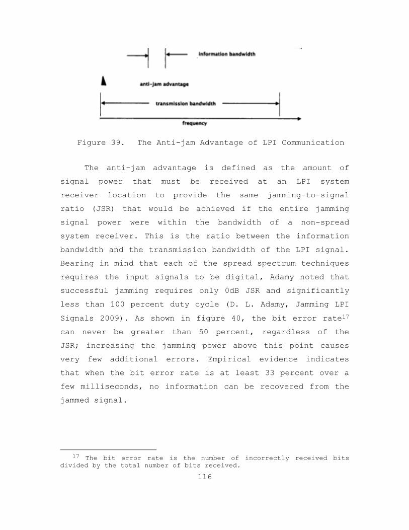
116

Figure 39. The Anti-jam Advantage of LPI Communication

The anti-jam advantage is defined as the amount of

signal power that must be received at an LPI system

receiver location to provide the same jamming-to-signal

ratio (JSR) that would be achieved if the entire jamming

signal power were within the bandwidth of a non-spread

system receiver. This is the ratio between the information

bandwidth and the transmission bandwidth of the LPI signal.

Bearing in mind that each of the spread spectrum techniques

requires the input signals to be digital, Adamy noted that

successful jamming requires only 0dB JSR and significantly

less than 100 percent duty cycle (D. L. Adamy, Jamming LPI

Signals 2009). As shown in figure 40, the bit error rate17

can never be greater than 50 percent, regardless of the

JSR; increasing the jamming power above this point causes

very few additional errors. Empirical evidence indicates

that when the bit error rate is at least 33 percent over a

few milliseconds, no information can be recovered from the

jammed signal.

17 The bit error rate is the number of incorrectly received bits

divided by the total number of bits received.

117

Figure 40. The Bit Error Rate in a Digital Receiver Cannot Exceed 50 Percent; a 0dB JSR Reaches this Level

of Errors;18

In the paragraphs to follow, we present the latest

trend in jamming LPI.

D. JAMMING

1. FSK

For FSK radars, the anti-jam advantage depicted in

figure 39 is based on the assumption that the jammer knows

only the full hopping range and must spread its jamming

power over that full frequency range. Denk provides an

interesting example to illustrate this: assume an FSK radar

that has a 2000 frequency hopping sequence which is random

or unknown to the ES receiver. The FSK radar can be said to

have a jamming advantage of 2000, which converts to 33dB.

This means that it takes 33dB more jammer power to achieve

a given JSR against this frequency hopper than would be

required if it were a fixed-frequency conventional radar.

18D. L. Adamy, Jamming LPI Signals 2009

118

Denk argues that the most effective jamming technique

for FSK is “follower jamming”, which entails a detection of

the frequency of each hop and then jamming on that

frequency (follower). As Adamy notes, this method requires

a sophisticated and extremely fast frequency measurement

technique in order to deny the enemy the transmitted

information in each hop (D. L. Adamy, EW 101: A First

Course in Electronic Warfare 2001). An extra consideration

is the fact that the frequency hopping sequence of FSK

radar is unknown and appears random to the ES receiver.

Unless this frequency sequence is solved, the possibility

of a jammer following the changes in frequency is highly

remote (Denk 2006, 99).

2. PSK

Phase coded signals can be affected mostly by VGPO-

type techniques.19 If the jammer introduces an additional

Doppler shift, this will be interpreted by the radar as an

additional phase shift, causing a spreading of the received

signal and thus a decrease in the effective processing gain

(Denk 2006, 93). If the Doppler shift is enough, a

corresponding loss of integration gain within the radar

processor should be expected (Denk 2006, 93; McRitchie and

McDonald 1999).

McRitchie and McDonald suggest that range bin masking

should also be quite effective. They argue that if a

section of the radar waveform recorded by DRFM or repeater

19VGPO is a method of capturing the velocity gate of a Doppler radar and moving it away from the skin echo. It is similar in essence to the RGPO, but is used against CW or Doppler velocity tracking radar systems. The CW or pulse Doppler frequency, which is amplified and retransmitted, is shifted in frequency (velocity) to provide an apparent rate change or Doppler shift.

119

is used by the jammer as its transmit waveform, the

truncation will cause an increase in the sidelobe levels of

the processed return. Total signal loss may occur as a side

effect of the merging of the sidelobes20; however, this will

degrade the SNR of the true target return, thus causing a

loss in processing gain (McRitchie and McDonald 1999).

3. FMCW

The main characteristic of FMCW radars that renders

them difficult to detect is their wideband waveforms.

Potential jammers have a significant problem measuring the

waveform parameters with sufficient accuracy to match the

jamming waveform (Pace 2004, 455). The situation is

exacerbated in a real-world environment, where an FMCW

radar operates among several radar systems in the same

frequency band. An extra difficultly derives from the

deterministic aspects of the FMCW radar. According to Pace,

the fact the return target signature has a form that can be

predicated (deterministic) provides the FMCW with

significant suppression capabilities of many interfering

waveforms that are uncorrelated (Pace 2009, 455).

Nevertheless, if the modulation period mt and

modulation bandwidth ΔF can be determined, then coherent

deception jamming is feasible and very effective, since the

jammer waveform looks like the radar waveform (Pace 2004,

455). Relevant literature suggests two major coherent

deception EA techniques:

20 According to Denk, the merging of the sidelobes can create a

threshold problem; in Aytug Denk, Detection and Jamming Low Probability of Intercept (LPI) Radars, Master's Thesis, Electronic Warfare, Naval Postgraduate School (NPS) (Monterey: NPS, 2006), p.93.

120

The first is by producing false range targets. In an

FMCW radar, this can be achieved by slightly shifting the

return frequency. Such a shift is expected to create an

equivalent shift in the apparent range of the signal as it

passes through the radar processor.

The second coherent EA technique is VGPO. Employed in

most Deceptive Electronic Countermeasure (DECM) systems,

VGPO signals repeat a frequency-shifted replica of the

received radar signal, initially programmed so that the

repeated signal is within the passband of the Doppler

filter containing the target return. This is designed to

allow the jammer to capture the Doppler filter containing

the target through the radar’s automatic gain control (AGC)

action. The repeated jammer signal is then swept in

frequency until the maximum expected Doppler frequency of

the radar is achieved. Then the repeated signal is switched

off, forcing the victim radar to reacquire the target

(Schleher 1999, 22).

Adamy suggests two approaches: the first requires

prediction of the frequency-versus-time characteristics of

the signal and the use of a jammer to direct energy to the

receiver at the same frequency as the FM signal it is

attempting to receive. This will allow the maximum jammer-

to-signal ratio (JSR) to be achieved for any given jammer

power and jamming geometry (D. L. Adamy 2001).

The second approach is to cover all or part of the

modulation range with a broadband jamming signal. This

jamming technique focuses the jamming power over a fraction

of the frequency modulation range that will allow the JSR

ratio in the jammed portion to cause a high rate of bit

121

errors in the digital modulation which is carrying the

signal’s information. The fraction of the jammed range

depends on the jammer power, the effective radiated power

of the modulated transmitter, and the relative ranges of

the transmitter and the jammer to the jammed receiver.

Noting that the SNR in the LPI receiver is already at

quite a low value, McRitchie and McDonald propose that a

narrow band Doppler noise may also be quite effective. A

Digital RF Memory (DRFM) can be used to focus the available

power of the jammer and inject Doppler noise only a few KHz

wide, matching to the instantaneous bandwidth of the FMCW

radar (McRitchie and McDonald 1999).

In the following table, we present the currently

deployed EA systems with the caveat that a measure of

effectiveness against LPI assets is unavailable in present

literature.

122

Platform Function Characteristics

ALQ-99E EA-6B, EF-111A Support Search Radar Jamming, 10 transmitters, analysis

receivers, directional antennas

ALQ-162B A-4, A-6, A-7, F-

4, F-14, F-18

Self-

protection

Coverage through I/J band, 1-kW peak power, 4%

to 5% duty, track radar jamming, typical 60-

degree fore/aft coverage, repeater transponder

modes

ALQ-136 Army Helicopters Self-

protection

I/J-band jammer, AA artillery radar jammer,

threat programmable

ALQ-131 F-16C, F-111, A-7,

A-10, F-15, F-4

Self-

protection

Dual mode pod jammer, CVR/ SHR analysis

receiver, phased array

ALQ-161 B-1B Self-

protection

Coverage through I band, search and track radar

jamming, monopulse and Doppler radar jamming,

software controllable, phased array

ALQ-162

(shadowbox)

F-16C, F-18, RC-

12D, RV-1D

Self-

protection

CW jammer, chopped repeater lightweight, threat

programmable, +60 degree switchable coverage

ALQ-165

(ASPJ)

F-16C, F/A18, F-

14, AV-8B

Self-

protection

Covered frequency range in two bands, pulse/CW

capability, analysis receivers, threat

programmable

ALQ-135

(TEWS)

F-15C Self-

protection

High powered transmitters, power management,

integrated with ALR-56C

123

Platform Function Characteristics

ALQ-172 B-52G/H Self-

protection

Track/search radar jamming, steerable jam beams,

software programmable, phased array antenna,

monopulse radar jamming

ALQ-184 (V) F-4, F-15. F-16,

A-7, A-10, F-111

Self-

protection

Pod jammer, Rotman lens, medium power miniature

TWTs, transponder and repeater jamming, high ERP

SLQ-32V (3) Ships Self-

protection

Lens fed array, crystal video and IFM receivers,

medium power miniature TWTs, tactical display,

transponder and receiver jamming, high ERP

Table 8. Modern EA Systems21

21Schleher 1999, 145.

124

THIS PAGE INTENTIONALLY LEFT BLANK

125

VI. NETWORKS AND NETCENTRIC WARFARE (NCW)

A. INTRODUCTION

As with other sensors, LPI radar systems can be

networked together as part of a network-centric warfare

(NCW) architecture to gather and share surveillance and

targeting data. In the case of LPI systems, this capability

is “covert” in nature. In this chapter, we discuss the NCW

notion on the three-layer architecture suggested by Phillip

E. Pace: the information layer, the sensor layer, and the

weapons layer. To point out the centrality of the NCW

notion in the modern battlefield, our analysis commences by

distinguishing between the concepts of platform-centric

warfare and network-centric warfare. It is followed by a

quantification of the NCW operational value, where central

notions such as Connectivity Measure, Network Rich, and

Network Richness are introduced.

B. NETWORK-CENTRIC WARFARE

Network centric warfare is defined as military

operations that exploit state-of-the art sensor information

and network technologies to integrate widely dispersed

human decision makers, weapons, situation and targeting

sensors, and forces into a highly adaptive comprehensive

system to achieve unprecedented mission effectiveness (Pace

2009, 320).

In a platform-centric architecture, a single asset is

the epicenter of operations. Peripheral weapons, each with

its own sensor(s) establish what Pace calls a “stovepipe

communication system,” transmitting the data back and

126

forth. The numerous platforms needed in architectures of

this type limit the Command and Control (C2) capabilities

as well.

Evolving from the platform-centric concept, NCW

integrates a distributed system of C2, sensors and weapons

into a grid, in order to collect, process, and disseminate

an uninterrupted flow of data among the various nodes. Its

main characteristic is the exponential effect it has on the

combat power of the overall architecture: for N number of

nodes, it gives a total force value of 2N , compared to N

for a platform-centric system (Pace 2009, 321).

C. NCW REQUIREMENTS

Among the several prerequisites for establishing a

viable NCW operation, bandwidth is arguably the most

central: next to a wideband transmit/receive capability to

sustain the compression and transportation of large amounts

of data, a wideband Local Area Network (LAN) that will

process and distribute the data to the various sensors and

weapons is required. Along with bandwidth requirements, the

issue of information processing capability and information

management is also critical. Having these elements in mind,

several questions arise regarding the formation of an NCW

architecture (Pace 2009, 322):

• How do different degrees of networking affect the

strategic, operational and tactical outcome?

• What is the optimal network topology (physical,

virtual, arrangement of nodes)?

• How will the network impact the C2?

127

• What is the correct balance of sensors, shooters

and network technology?

• How can degradation of network processing be

quantified (i.e., in the event of an electronic

attack)?

As Pace notes, the complexity of the relationships

between the network space and the battle space makes

answering these questions difficult; a schematic depiction

is provided in Figure 41.

Figure 41. Relationship Between Network Space and Challenges22

To establish a solid theoretical foundation prior to

quantifying the metrics for information grid analysis, we

provide the definitions of the various NCW requirements.

22Pace 2009, 323.

128

1. Situational Awareness

Situational awareness is “the ability to have accurate

real time information of friendly, enemy, neutral and non-

combatant locations; a common, relevant picture of the

battlefield scaled to specific levels of interest and

special needs” (Stein, Garska and McIndoo 2000).

In practice, situational awareness is built by

continuous snapshots that are gathered from the theater of

operations and sent to the C2 center. The refreshing of the

snapshots, deriving mainly from the number of the nodes and

their processing capabilities, results in greater

information flow; consequently, situational awareness is

mainly determined by information processing capability

(Kruse, Adkins and Holloman 2005).

2. Maneuverability

In the NCW context, maneuverability is defined as the

capability to perform a strategic or tactical movement. To

clarify this generic definition, Pace approaches the

maneuverability concept considering three of its

properties: speed, safety and cost. The effect of speed on

maneuverability is obvious—the greater the speed, the

greater the capability of movement. Safety has the opposite

effect, as all additional precautions reduce the tempo.

Last but not least, high maneuverability networks require

complex, and thus, costly assets and structure. Studying

the various aspects of battle topology situational

awareness, Chen and Pace schematically depict their

interaction with maneuverability as shown in Figure 42.

129

Figure 42. Maneuverability23

3. Decision Speed and Operational Tempo

The notion of the Observation-Orientation-Decision-

Action (OODA) loop was first developed by John Boyd in his

monumental work entitled A Discourse on Winning and Losing,

commonly known as “The Green Book” (Boyd 1987). A central

concept in military strategy, the OODA loop is shown in

Figure 43.

Figure 43. OODA Loop

To quantify the maximum network operational tempo—an

important attribute when considering the fusion of netted

radar data—Pace examines each phase separately. In the

observation-orientation phase, the characteristic tempo Tλ ,

is defined as “the speed in which the situational awareness

is processed in order to orient (or adjust) the force to

23Chen and Pace 2008.

130

the current situation” (Pace2009, 323). Moving to the

decision phase, the decision tempo cλ refers to the “speed

to make a decision for action”, and is mathematically

described as the sum of the characteristic tempo Tλ and the

deployment tempo dλ . After the deployment, the overall speed

at which the situational response is made is the sum of the

characteristic tempo and a fighting tempo fλ . The maximum

operational tempo ΛOODA is the defined as the inverse of the

maximum frequency to complete the OODA cycle.

4. Agility

Highly affecting the operational tempo, agility in the

NCW context is defined as “the ability of an organization

to sense and respond to advancement opportunities in order

to stay ahead and competitive in a turbulent battlefield

quickly.” To better convey the notion of agility, Pace

graphically depicted the interrelation between operational

tempo and force agility as in figure 44.

Figure 44. Operational Tempo vs. Force Agility24

24Pace 2009, 325.

131

Pace did not provide any formulas or other means to

quantify agility, which, along with maneuverability and

situational awareness, remain abstract terms in relevant

literature.25 A careful study of the definition and Figure

46 indicate that the higher the operational tempo, the

higher the agility of the force.

5. Lethality

Another abstract term utilized by Pace to assess the

various NCW requirements is lethality, which is defined as

“the ability to damage an enemy” (Pace 2009, 325).

Obviously the use of the term is not constrained to the NCW

realm but can also pertain to non-netted configuration,

that is asset-to asset- confrontation. For the purpose of

this thesis, lethality, where used, shall represent a

measure of jamming effectiveness against LPI assets,

whether in netted configuration or not.

D. METRICS FOR INFORMATION GRID ANALYSIS

As previously discussed, the total capability of the

network is greatly affected by the number of nodes.

However, quantification of this capability has been

difficult to achieve as, among other issues, each node

differs significantly from each other; consequently,

relevant analysis has often provided misleading results

(Ling, Moon and Kruzins 2005). In this section, we

introduce the latest metrics designed to quantify the

general value inherent in the information network topology.

25 Our research indicates that these terms appear only in Philip

Pace’s work: Phillip E. Pace, Detecting and Classifying Low Probabilty of Intercept Radars, 2nd Edition (Norwood, MA: Artech House, 2009).

132

1. Generalized Connectivity Measure

The generalized connectivity measure of a network of

sensors or weapons is defined as the sum of the value of

all the nodes and their connections scaled by the lengths

of the routes and their directionality (P. E. Pace, 2009,

325). Its mathematical expression is (Ling, Moon and

Kruzins 2005):

( ) ( ) ( ),Τ Ν ΝΝ

,

1 1 1Κ , 6.1

µ µ νµ ν

M µ γµ ν γ

C t t L d t= = =

=∑ ∑∑

Where:

TN : The number of nodes in the network

µN : The total number of nodes connected to the node μ

,µ νN : The total number of possible routes26 connecting the

pair of nodes µ and ν .

( )µK t : The capability value of node μ; ( ) 0µK t ≥

,µ νγL : The information flow parameter of the route γ

connecting nodes µ and ν : , 0µ νγL ≥ . It depends on the length

of the route and it is also a function of time. The

functional dependence of ,µ νγL on the length of the route δ

(number of links27), can be simplified by separating it into

a time independent component, and a time dependent

coefficient, scaled by the route length d raised to the

26 The term route refers to the possible connection from one node to

another. 27 The term link represents the direct connection between any two

nodes. One route contains one or more links.

133

power ξ . The value of

( ),µ ν

γF t , is a minimum of zero and

reaches a maximum of one the route γ .. Eqn. (6.1) then

becomes:

( ) ( ) ( )( )

,Τ Ν Ν ,Ν,

1 1 1Κ 6.2

µ µ ν µ νγµ ν

M µ γ ξµ γ γ γ

F tC t t Ld= = =

=∑ ∑ ∑

2. Reference Connectivity Measure

Reference connectivity measure refers to a fully

connected network, that is, a network that has all nodes

fully connected with bidirectional links where each of the

nodes has a capability value of

1µK = : (Ling, Moon and

Kruzins 2005). Consequently, the resulting reference

network has the highest connectivity measure of any network

with the same number of nodes.

The reference connectivity measure depends only on the

total number of nodes. Its mathematical expression is:

( ) ( )( )2 3 2 121 1 6.32 1T TR T

M T TT

N NNC N N N⎛ ⎞− − …⋅ ⋅−⎜ ⎟= − + +…+⎜ ⎟−⎝ ⎠

The term ( )1T TN N − represents the number of possible

connections in a given network with TN nodes. The numerator

in each of the terms inside the square brackets is the

number of possible routes of the length given in the

denominator.

3. Network Reach

Network reach is dimensionless term created to provide

a means of normalizing the connectivity measure (Ling, Moon

134

and Kruzins 2005). As Pace notes, normalization by the

reference network allows us to investigate the varying

degrees of network connection, the non-identical

nodes/links and the effect of broken symmetries (Pace 2009,

329). The latter becomes significant in cases of reduced

network performance, such as when evaluating the effect of

EA on the whole architecture. The formula for network reach

is (Ling, Moon and Kruzins 2005):

6.4MR R

M

CI C=

4. Extended Generalized Connectivity Measure

The concept of the generalized connectivity measure

was developed in order to analyze network architectures

with routes not able to maintain full capability in the

flow of sensor information (Chen and Pace June 2008). In

the network shown in Figure 45, the limited capability

value of nodes 2 ( )2 0.5K = and 3 ( )3 0.5K = constrain the

information flow when data follows the route: node 1→ node

2 →node 3.

Figure 45. Three-node Network Example

135

To account for this limitation, Pace suggests an

extended definition of connectivity measure as (Pace 2009,

333):

( ),Τ Ν Ν ,Ν

1 1 1

Κ 6.5µ µ ν

e

µ νγ γ

Mµ ν γ γ

FC t d= = =

=∑∑∑

Where:

γK : The µK with the lowest capability value (bottleneck) in

route γ .

γK considers the starting node and exchangers but not

the receiving node because in military networks, many nodes

only receive data, without equivalent processing capability

for transmitting.

Pace concludes that, by comparing MC to RMC , and by

disabling nodes in the reference and the real network and

recalculating both values, the robustness of network can be

quantified. This comparison can provide a clear

representation of the real network under attack (Pace 2009,

333).

5. Entropy and Network Richness

a. Entropy

The concept of entropy is central to our

analysis, as it is directly linked to the calculation of

the information rate λ. In information theory, entropy is a

measure of the uncertainty associated with a random

variable. The concept of entropy was analytically studied

by Claude E. Shannon, who, in his monumental 1948 work on

communication signals, studied entropy in the context that

136

quantifies the expected value of information contained in a

message. Applying Shannon’s approach to net-centric

architecture, we note that at each node, the data exchange

rate has a direct impact on the operational tempo of the

grid. Assuming a set of J possible sample values by:

1 2, , 6.6JS x x x= …

and assuming that the probability of the source output jx

is jp , the amount of information sent when the message

is transmitted is:

( ) ( )2 6.7jI j log p= −

where jp is the probability of transmitting the message.

Shannon’s entropy (or uncertainty) of the source is

described by the formula:

( ) ( ) ( )21

6.8J

j jj

H S E I j p log p=

= = −∑

The information rate of the source is then:

( )/ 6.9Hλ bits secT=

where T is the time required to send the message. A related

measure is the channel capacity or:

( )( )2 1 / 6.10C Blog SNR bits sec= +

where B is the channel Bandwidth and SNR the signal-to-noise power ratio (not in dB) at the receiver input

(Shannon 1948). Pace notes that the channel capacity can be

137

used as a unifying principle for both electronic attack

(EA) and electronic protection (EP) actions in EW: all EA

actions can be considered an attempt to reduce the

bandwidth of an adversary signal and/or to reduce the SNR

and all EP actions as an attempt to increase bandwidth

and/or increase SNR (Pace 2009, 333).

To demonstrate this, Pace provides three

examples:

Example 1: When an LPI emitter uses frequency

hopping as an EP measure, protection against jamming

necessitates a large total bandwidth; if the same emitter

wants to protect against interception only, then only a

small instantaneous bandwidth is required. In this case,

the large total bandwidth makes it difficult for the jammer

to set on the transmission frequency, thus limiting the

reduction in SNR to that provided by barrage jamming.

Example 2: Applying repeater or gate stealing EA

techniques requires a certain reduction of SNR within the

bandwidth of the victim’s receiver to be effective. The

corresponding EP technique might utilize a combination of

guards and filters to recognize and eliminate the unwanted

jamming signal, thereby protecting the SNR.

Example 3: To avoid adversary exploitation, a LPI

emitter uses a very large bandwidth with low average power

density, which reduces the probability of intercept.

However, the energy over the bandwidth can be summed to

extract the information from the signal. Therefore, the

transmitter compensates for the low SNR with increased

138

bandwidth to transmit the information at fast enough rates.

The jammer can achieve high SNRs only over small portions

of the bandwidth.

b. Network Richness

Within the sensor network, each node is able to

process the information at its own rate; by combining the

various node information rates, we can quantify the

network’s richness. The information rate Tλ of a node µ is

the rate at which the network information is processed by

the node. The minimum information rate

minµλ , of the node is

the minimum rate that information must be processed for

generating decision-level knowledge from the sensor network

data. From Shannon’s information entropy theory, the

knowledge function is defined as (Ling, Moon and Kruzins

2005):

( )

0,

, 6.11

1,

minµ µ

µ min minµ µ µmin

µµminµ min

µ µminµ

λ eλeλln λ λ eλλQ λeλln λ eλλ

⎧⎪ ≥⎪

⎛ ⎞⎪ ⎜ ⎟ < <⎪ ⎜ ⎟⎪ ⎝ ⎠= ⎨⎪ ⎛ ⎞⎪ ⎜ ⎟ = ≥⎪ ⎜ ⎟

⎝ ⎠⎪⎪⎩

Using the knowledge function, Ling et al. defined

the network richness QR as the average rate at which

information entropy (or knowledge) is generated from the

network shared data (Ling, Moon and Kruzins 2005):

( )ΤΝ

1 6.12 µ µµQ

T

λ Q λR N

==∑

139

Equation (6.12) leads us to two major

observations:

• If a node cannot provide data at a rate above

its minimum value , it degrades the overall

value ( )µ µλ Q λ .

• There is little advantage to generating sensor

data faster than knowledge can be generated and

absorbed.

6. Maximum Operational Tempo

The maximum information exchange rate of a network is

determined by the following factors:

• The number of nodes;

• The communication and sensor technologies

employed;

• The information data transfer rates, and

• The network topology.

To quantify this rate within an OODA loop, Pace

introduces the term characteristic tempo Τλ , a concept that

relates the network topology to its ability to gather

situational awareness. In a net-centric architecture

characteristic tempo is defined as the product of the

network reach RI and the network richness QR (Pace 2009,

336):

6.13T R Qλ I R=

140

Figure 46 shows the tempo parameters of the sensor

network OODA loop:

Figure 46. Time Spent in Each OODA Cycle Phase28

The variable 1Δt represents the time from observation

to orientation and is limited by the information exchange

time; 2Δt is the time from orientation to decision and is

dominated by the decision speed; 3Δt is the time from

decision to action and must be greater than the information

exchange time (command time) and deployment time; 4Δt is the

time from action to observation and is always greater than

the sum of information exchange time and fighting time.

The lower limits for each of the Δ it presented above are as follows:

1Τ

1Δ 6.14t λ≥

28Pace 2009, 336.

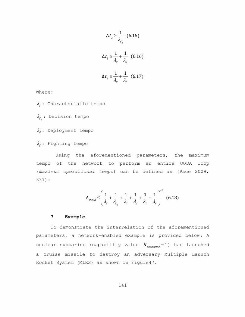
141

2

21Δ 6.15C

t λ≥

3Τ

1 1Δ 6.16d

t λ λ≥ +

4Τ

1 1Δ 6.17f

t λ λ≥ +

Where:

Tλ : Characteristic tempo

2Cλ : Decision tempo

dλ : Deployment tempo

fλ : Fighting tempo

Using the aforementioned parameters, the maximum

tempo of the network to perform an entire OODA loop

(maximum operational tempo) can be defined as (Pace 2009,

337):

2

1

Τ Τ Τ

1 1 1 1 6.181 1ΛOODAC d fλ λ λ λ λ λ

−⎛ ⎞⎜ ⎟≤ + + + + +⎜ ⎟⎝ ⎠

7. Example

To demonstrate the interrelation of the aforementioned

parameters, a network-enabled example is provided below: A

nuclear submarine (capability value

1submarineK = ) has launched

a cruise missile to destroy an adversary Multiple Launch

Rocket System (MLRS) as shown in Figure47.

142

Figure 47. Network Topology

To follow up with the damage report, a tactical UAV

flies to the target and a Global Hawk UAV covers the

intelligence, surveillance and reconnaissance (ISR)

component. Due to its limited connectivity and signal

rerouting options, the cruise missile capability value is

assumed to be 0.4cruiseK = .29 The Global Hawk also has a limited

rerouting capability and is given a capability value of

0.9HawkK = .30

Assuming each link to have a flow component of either

1 or 0. (i.e.,

1,0F L= = ), the reference connectivity measure

is:

29 Note its unidirectional link to the Global Hawk. 30In reality, no tactical UAV is fast enough to follow a cruise

missile; the choice of the assets is imaginary and aims at visualizing an operational scenario, not at providing a real-combat configuration.

143

( ) ( ) ( )

( ) ( ) ( )

2 321 1 2 34 2 4 34 24 4 1 1 322 3

T TR TM T T

R RM M

N NNC N N

C C

⎡ ⎤− ⋅ −−⎢ ⎥= − + + ⇒⎢ ⎥⎣ ⎦⎡ ⎤− ⋅ −−⎢ ⎥⇒ = ⋅ − + + ⇒ =⎢ ⎥⎣ ⎦

To calculate the network reach, we break our process

into five steps.

Step I: Calculating 1νFd∑ :

11 0N =

1 2 1 1 2 3 12 2N =

2

12 1 1 91 2 6

Fd = + =∑

1 2 1 1 3 2 13 2N =

3

13 1 1 91 2 6

Fd = + =∑

1 2 1 1 3 2 4 3

14 2N =

4

14 1 1 52 3 6

Fd = + =∑

Step II: Calculating 2νFd∑ :

1 2 3 2 2 2 1 3 3 1 4

21 3N =

1

21 1 1 1 111 2 3 6

Fd = + + =∑

22 0N =

144

1 2 2 2 3 1 23 2N =

3

23 1 1 91 2 6

Fd = + =∑

1 2 2 2 3 1 4 3

24 2N =

4

24 1 1 52 3 6

Fd = + =∑

Step III: Calculating 3νFd∑ :

1 2 3 3 3 3 1 2 4 31 3N =

1 1

31 1 2 91 2 6

Fd = + =∑

1 2 3 3 3 3 2 1 4 2 1

32 3N =

2

32 1 1 1 111 2 3 6

Fd = + + =∑

33 0N =

1 3 34 3N = 4

34 1 61 6

Fd = =∑

Step IV: Calculating 4vFd∑ :

1 2 3 4 4 4 1 3 3 1 2

41 3N =

1

41 1 1 1 111 2 3 6

Fd = + + =∑

145

1 2 3 4 4 4 1 3 3 2 2 1

42 3N =

2

42 2 1 82 3 6

Fd = + =∑

1 2 3 4 4 4 3 1 1 3 2

43 3N =

3

43 1 1 1 111 2 3 6

Fd = + + =∑

44 0N =

Step V: The network reach will be:

Τ ΝΝ 4

1 1

1 2 3 4

1 2 3 4

1 1 Κ

1

1 23 25 26 300.9 0.6 1 0.4 0.383832 6 6 6 6

µν µνγ

R M R µR Rµ γM M

ν ν ν ν

R RM

R R

FI C I dC C

F F F FI K K K Kd d d dC

I I

=

= =

⎡ ⎤⎢ ⎥= ⇒ = ⇒⎢ ⎥⎣ ⎦

⎡ ⎤⇒ = + + + ⇒⎢ ⎥

⎣ ⎦

⎡ ⎤⇒ = ⋅ + ⋅ + ⋅ + ⋅ ⇒ ≅⎢ ⎥

⎣ ⎦

∑ ∑

∑ ∑ ∑ ∑

This example manifests the centrality of two elements

in the network reach concept regarding a net-centric

architecture: the number of nodes and the capability value.

The number of nodes affects the network reach, and thus the

overall performance of the network by means of the

parameter µνFd∑ ; if we increase the number µ of nodes, the

square bracketed term in the previous relationship will

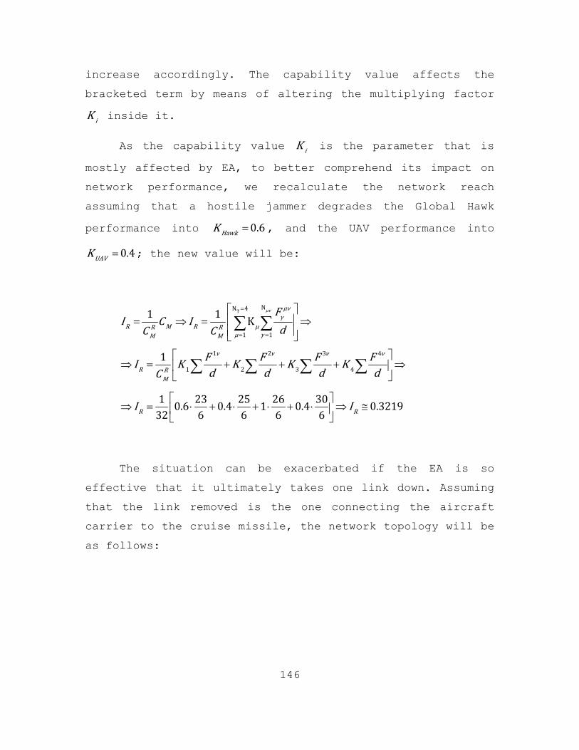
146

increase accordingly. The capability value affects the

bracketed term by means of altering the multiplying factor

iK inside it.

As the capability value iK is the parameter that is

mostly affected by EA, to better comprehend its impact on

network performance, we recalculate the network reach

assuming that a hostile jammer degrades the Global Hawk

performance into 0.6HawkK = , and the UAV performance into

0.4UAVK = ; the new value will be:

Τ ΝΝ 4

1 1

1 2 3 4

1 2 3 4

1 1 Κ

1

1 23 25 26 300.6 0.4 1 0.4 0.321932 6 6 6 6

µν µνγ

R M R µR Rµ γM M

ν ν ν ν

R RM

R R

FI C I dC C

F F F FI K K K Kd d d dC

I I

=

= =

⎡ ⎤⎢ ⎥= ⇒ = ⇒⎢ ⎥⎣ ⎦

⎡ ⎤⇒ = + + + ⇒⎢ ⎥

⎣ ⎦

⎡ ⎤⇒ = ⋅ + ⋅ + ⋅ + ⋅ ⇒ ≅⎢ ⎥

⎣ ⎦

∑ ∑

∑ ∑ ∑ ∑

The situation can be exacerbated if the EA is so

effective that it ultimately takes one link down. Assuming

that the link removed is the one connecting the aircraft

carrier to the cruise missile, the network topology will be

as follows:

147

Figure 48. Network Topology after EA

Since the number of nodes is unaltered, the reference

connectivity measure remains the same:

( ) 32RMC EA =

To calculate the new network reach, we work similarly:

Step I: Calculating 1νFd∑ :

11 0N =

1 2 1 1 2 3 12 2N =

2

12 1 1 91 2 6

Fd = + =∑

1 2 1 1 3 2 13 2N =

3

13 1 1 91 2 6

Fd = + =∑

148

14 0N =

Step II: Calculating 2νFd∑ :

1 2 2 2 1 3 21 2N =

1

21 1 1 91 2 6

Fd = + =∑

22 0N =

1 2 2 2 3 1 23 2N =

3

23 1 1 91 2 6

Fd = + =∑

24 0N =

Step III: Calculating 3νFd∑ :

1 2 3 3 1 2 31 2N =

1

31 1 1 91 2 6

Fd = + =∑

1 2 3 3 2 1 32 2N =

2

32 1 1 91 2 6

Fd = + =∑

33 0N =

34 0N =

Step IV: Calculating 4νFd∑ :

1 4 41 2N = 1

411F

d =∑

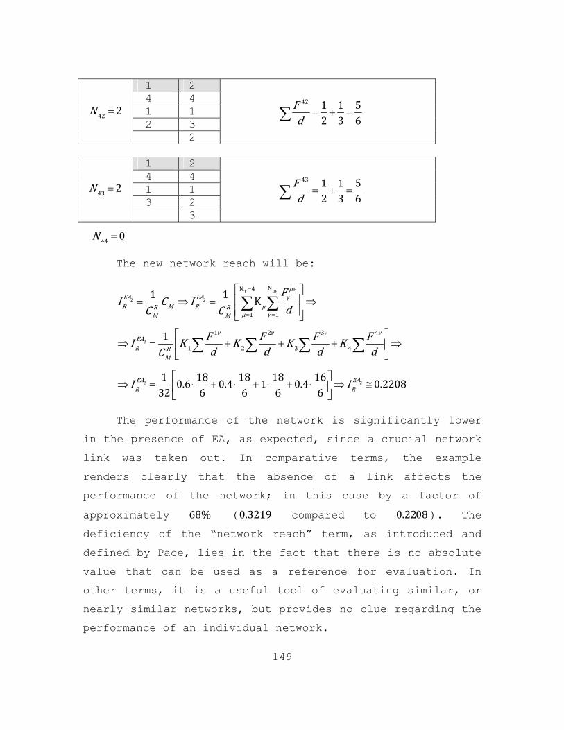
149

1 2 4 4 1 1 2 3

42 2N =

2

42 1 1 52 3 6

Fd = + =∑

1 2 4 4 1 1 3 2

43 2N =

3

43 1 1 52 3 6

Fd = + =∑

44 0N =

The new network reach will be:

Τ2 2

2

2 2

ΝΝ 4

1 1

1 2 3 4

1 2 3 4

1 1 Κ

1

1 18 18 18 160.6 0.4 1 0.4 0.220832 6 6 6 6

µν µνEA EA γR M R µR R

µ γM M

ν ν ν νEAR R

M

EA EAR R

FI C I dC C

F F F FI K K K Kd d d dC

I I

=

= =

⎡ ⎤⎢ ⎥= ⇒ = ⇒⎢ ⎥⎣ ⎦

⎡ ⎤⇒ = + + + ⇒⎢ ⎥

⎣ ⎦

⎡ ⎤⇒ = ⋅ + ⋅ + ⋅ + ⋅ ⇒ ≅⎢ ⎥

⎣ ⎦

∑ ∑

∑ ∑ ∑ ∑

The performance of the network is significantly lower

in the presence of EA, as expected, since a crucial network

link was taken out. In comparative terms, the example

renders clearly that the absence of a link affects the

performance of the network; in this case by a factor of

approximately 68% (0.3219 compared to 0.2208 ). The

deficiency of the “network reach” term, as introduced and

defined by Pace, lies in the fact that there is no absolute

value that can be used as a reference for evaluation. In

other terms, it is a useful tool of evaluating similar, or

nearly similar networks, but provides no clue regarding the

performance of an individual network.

150

E. NETTED LPI RADAR SYSTEMS

Despite recent advantages in mono-static radar systems

(collocated single transmitter and receiver), two major

disadvantages are inherent: they offer little to counter

stealth technology and they only offer a single perspective

for each radar (Hume and Baker October 2001). The

development of stealth technology has primarily been aimed

at defeating the mono-static radar by the use of absorbing

materials and non-reflective structural designs that

minimize the scattered energy reflected into the

hemisphere, in the direction from which the signal arrives.

The limited energy returned to the emitter from the stealth

target makes it very difficult to detect the target. In

addition, due to terrain obscuration, ground based or low-

flying mono-static radar systems often do not have a line

of sight (LOS) to the target and therefore cannot provide

detection.

Due to this single perspective, the richer information

contained in multiple perspectives is missed. When a number

of cooperative radar systems are distributed spatially and

networked together, they can provide the opportunity to

view the target from a number of different aspect angles.

In multi-frequency radar networks, each radar performs a

significant amount of local preprocessing. Outcomes of the

local preprocessing can then be delivered to a central

processor through a communication link. The preprocessing

limits the amount of information that needs to be passed on

to make a final detection decision. These systems use

151

different frequencies to cope with interference rejection,

but each receiver is unable to process the information from

all transmitters.

Netted radar systems, sometimes referred to as

Multiple-Input-Multiple-Output (MIMO) radar systems,

consist of a number of distributed radar systems (transmit

and receive sensors) each having the ability to transmit

independent orthogonal waveforms (to avoid interference)

and the ability to receive and process synchronously all

waveforms that are transmitted. Figure 49 depicts an

example of a MIMO netted radar system with three radar

nodes connected by a network:

Figure 49. Three-node MIMO Netted Radar System31

All three radars have acquired and are tracking the

target with their antenna beams. The LPI Emitters R1, R2,

31Pace 2009, 346.

152

and R3 each transmit a different waveform but receive and

process all three waveforms that are collected from the

target. The use of the network allows each node to share

its target information non-coherently (using orthogonal

waveforms) or coherently. The implementation of networked

radar systems has become feasible due to recent advantages

in large bandwidth wireless networks, high capacity

transmission lines, multichannel electronically scanned

antennas, high-speed, low-cost digital processors, and

precise synchronization systems (Teng et al. 2007).

153

VII. NETTED RADAR SYSTEMS -- ADVANTAGES AND DISADVANTAGES

A. MULTISITE RADAR SYSTEMS CATEGORIZATION

A Multisite Radar System (MSRS) is one that includes

several spatially separated transmitting, receiving and/or

transmitting-receiving facilities where information of each

target from all sensors are fused and jointly processed

(Chernyak 1998, 3). This definition covers both multi-

static radars (radars that have one transmitter and several

receiving stations spatially separate from each other) as

well as multi-radar systems that are comprised of many

transceiver radars spatially separate from with each other.

The latter is also called a netted radar system.

Netted radar systems can be realized by the

interconnecting different types of transceiver radars. This

thesis examines netted radar systems realized by

interconnecting several LPI radars (netted LPI radars).

The two main differences between netted LPI radar

systems and a single LPI radar are the several spatially

separated stations (LPI radars) and the fusion (joint

processing) of the target information. These two features

give netted LPI radars their main benefits.

MSRSs can be further classified by the following

attributes (Chernyak 1998, 3-6).

1. Type of Targets of Interest

These can be divided into active, passive and

active/passive. This classification is heavily dependent on

the characteristics of the target of interest. If the

154

target is a radiating target then it can be served by a

passive MSRS; if the target is non-radiating it can be

served by an active MSRS. The active/passive MSRS can serve

both radiating and non-radiating targets.

2. The Degree of Spatial Coherence

The spatial coherence of an MSRS is the ability to

maintain a strong dependence between signal RF phases

between separated stations32. Spatial coherence of an MSRS

is actually the phase stability of its equipment. MSRSs are

classified into three categories.

a. Spatially Coherent MSRSs

These provide almost full utilization of the

electromagnetic field spatial structure. They require

precise time synchronization, precise frequency control and

precise phase control; this demands they be implemented

with many stations (several dozen or more), creates

difficulties in the inter-station phasing implementation,

and are very complicated and expensive to build. To build

such MSRSs, usually the designers keep the station base-

length small, which leads to the loss of critical waveform

information by the MSRSs and thus reduces the advantages of

the spatial coherence.

b. Short-Term Spatial Coherent MSRSs

In these MSRSs the equipment phase stability is

maintained within short time intervals, mainly for the used

32 We must distinguish between the spatial coherence of the MSRS and

the spatial coherence of the signal at the inputs of the MSRS receiving stations. The latter depends on the baselengths between stations, signal wavelength, target size and fluctuation of the propagating medium.

155

signal duration at least. The inter-station phase shifts

are assumed to be random and mutually independent and in

this context they do not contain useful information. The

joined signal processing in these kinds of MSRSs can use

all the information contained in the signal complex

envelopes in plots and tracks from different stations.

Consequently they do not require inter-station phase

control, but they require time synchronization and

frequency control. These facts permit their implementation

with a few stations only, reducing complexity and

implementation cost compared with the spatially coherent

system. The resolution and accuracy characteristics no

longer depend on carrier frequency, but on frequency

bandwidth. The loss of information--compared to the

spatially coherent system--can be compensated for by

increasing the baselines.

c. Spatially Incoherent MSRSs

In these MSRSs, the inter-station phase

information and its changes in time are not used. They

utilize information contained only in signal real envelope

relations, plots and tracks from separated stations. Only

time synchronization of the separated stations is

necessary. These types of MSRSs are much simpler than the

other types of MSRSs but due to the loss of the phase

information there are certain power and information losses.

Of course, the spatial incoherence does not rule out the

temporal coherence of each station before information

fusion (e.g., measurement of Doppler shifts and target

156

radial velocity in each radar). Table 9 summarizes the

characteristics of the degree of spatial coherence design

criterion of an MSRS.

MSRS Type Advantages Disadvantages

Spatially coherent

• Full utilization of the EM field spatial structure.

• Require precise time synchronization, frequency control and phase control • Complicated. • Expensive. • Require many stations (radars).

Short term Spatially coherent

• Utilize the information contained in the signal complex envelopes • Do not require inter-station phase control • Implementation with a few stations only • Reduced complexity and implementation cost compared with the spatially coherent ones

• They require precise time synchronization and frequency control.

Spatially incoherent

• Utilize information containing only in signal real envelope • Only time synchronization of the separated stations is necessary • They are simpler than the other types of MSRSs • They have the least cost compared to the other types of MSRSs.

• There are certain power and information losses due to the loss of the phase information.

Table 9. Degree of Spatial Coherence Summary

157

3. Information Fusion Level

MSRSs can be categorized into four classes. In each

class, both analog and digital transmission lines can be

used.

a. Radio Signal Integration Level

All signals, noise and interference are subject

to joint processing. Information is either transmitted

immediately by the stations as raw data or after

preliminary linear filtering. This type of fusion level

requires high capacity wideband transmission lines.

b. Video Signal Integration Level

After phase elimination at each station, all

signals, noise and interference are subject to joint

processing. The required capacity of the transmission lines

is slightly reduced but there are certain power and

especially information losses. This type of fusion leads to

no spatial coherence, which is why it’s seldom used.

c. Plot33 Integration Level

There is initial information processing at the

station level (signal thresholding and parameter

estimation) and only useful information is transmitted for

fusion. The partial processing done at the stations has to

do with the preliminary decision of existence or not of a

target; the final decision is made at the fusion center

33 A plot is a result of individual target detection and parameters

measurement or a measurement of target’s coordinates and their derivatives when an “instantaneous” target state is estimated without taking into account previous measurement results.

158

(decentralized or distributed detection). This in effect

reduces greatly the required capacity of the transmission

lines.

d. Track Integration Level

Apart from the initial information processing at

the station level, secondary information processing occurs

resulting in target track information. Those track data are

then transferred to the fusion center where false tracks

are eliminated and true track parameters are estimated more

accurately. The required transmission line capacity is

similar to the plot integration level. Table 10 summarizes

the characteristics of the information fusion level design

criterion of an MSRS.

159

MSRS Type Advantages Disadvantages

Radio signal • No information losses.

• Require high capacity transmission lines. • Require complicated fusion processing.

Video signal • All information but phase is transmitted to the fusion center.

• Require high capacity transmission lines but with less capacity than those for radio signals. • There cannot be spatial coherence with this type of fusion.

Plot • Only useful information is transmitted to the fusion center (plot). • Require low capacity transmission lines.

• Reduced power and information characteristics of the MSRS.

Track • Only track data are transmitted to the fusion center. • Require low capacity transmission lines.

• Reduced power and information characteristics of the MSRS

Table 10. Information Fusion Level Summary

4. Degree of Autonomy of Signal Reception

MSRSs can be categorized into three classes; in each

class both analog and digital transmission lines can be

used.

a. Independent (Autonomous) Signal Reception

Stations (radars) of this MSRS type are designed

to receive scattered signals from targets illuminated by

the same radar only. These are generally spatially

incoherent MSRSs that use the plot or track level of

fusion. They are often called netted radar.

160

b. Cooperative Signal Reception

Stations (radars) of such an MSRS are designed to

receive and process echoes from targets illuminated by any

radar or MSRS station. They provide better power and

information characteristics than do independent ones. An

example of such an MSRS is a multi-static radar with one

transmitting and many receiving stations.

c. Independent - Cooperative Signal Reception

Stations (radars) of such an MSRS are designed to

do both independent and cooperative signal reception.

5. Station Location and Mobility

MSRSs can be categorized into five classes.

a. Ground-Based MSRSs With Stationary Stations

These systems, even though they may be comprised of

mobile ground stations, require the stations’ positions to

be fixed during MSRS operation.

b. Ground-based MSRSs With Mobile Stations

These systems are comprised of mobile ground

stations that can change positions during the MSRS

operation.

c. Transmitter (or Receiver) on Platforms, Receiver (or Transmitter) Ground-based.

These systems have one part of the MSRS

(transmitter or receiver) on a platform (i.e., aircraft,

satellite) and the other (receiver or transmitter

respectively) fixed on the ground.

161

d. All Stations on Platforms

All stations (transmitters, receivers or

transceivers) are placed on platforms (aircraft, vehicles,

satellites).

e. Shipborne

All stations (transmitters, receivers or

transceivers) are placed on ships.

B. ADVANTAGES OF MULTISITE RADAR SYSTEMS

The advantages of a MSRS system over a mono-static

radar or a number of radars that are not integrated in a

system are briefly discussed here (Chernyak 1998, 9-21;

Pace 2009).

1. Capability to Form Coverage Area of Required Configuration for Expected Environments

It is apparent that the actual geometry of an MSRS

(that can also be tailored to each specific application),

in combination with the fusion algorithms that are used,

gives an area coverage advantage over a mono-static radar

or a system of radars that are not integrated.

2. Power Advantages

Adding transmitting and/or receiving stations to a

mono-static radar (and thus forming an MSRS) upgrades the

total power and/or sensitivity of the system. There are

also some other significant advantages in the case of

cooperative signal reception (as described in paragraph 4.b

above), where if the baseline distances are sufficiently

long or when the target is illuminated by sufficiently

separated stations, there is a significant power gain due

162

to fluctuation smoothing. That gain can also be obtained by

MSRSs that apply independent signal reception (as described

in paragraph 4.a above) but use different carrier

frequencies.

3. Detection of Stealth Targets

Stealth technology primarily aims to defeat the mono-

static radar by the use of radar absorbing materials (RAM)

and non-reflective structural designs that minimizes the

scattered energy reflected back into the hemisphere from

which the signal arrives. Most stealth assets are designed

to hide their front aspect angle from radar. Having a

netted radar system (MSRS) (which covers an area from

various aspect angles), can in effect negate the advantage

of a stealth asset because some number of the stations

comprising the MSRS will view the target from a number of

different aspect angles.

4. High Accuracy of the Position Estimation of a Target

An MSRS can estimate target coordinates through range

measurements from several spatially separated stations

(either several mono-static netted radars or multi-static

radar system). As one can see in Figure 50, for the

respective MSRS category (netted mono-static and multi-

static) the resulting error after the fusion is the

intersection of the individual errors.

163

Figure 50. Netted Mono-static (left) Multi-static (right) Increase of Angular Coordinate Measurement

Accuracy34

The formulas for calculating this error for the two

cases are:

2 2 7.1sinθ R Reff

σ σ σL θ L= ≈

Σ22 2 7.2R

θ Reff eff

σσ σ L L= ≈

Where:

θσ : RMS error of angle estimation in the bi-static plane

Rσ : RMS error of range measurements

L : Baselength (distance between radars)

effL : Effective baselength

34Chernyak 1998, 10.

164

ΣRσ : RMS error of range sum measurements

c : Speed of light

Tσ : RMS error of time arrival

Equations (7.1) and (7.2) suggest that if the range

measurements are very accurate (e.g., wideband signals such

as FMCW are used and thus Rσ decreases) or the stations

have large baselengths ( effL increases) we can achieve a very

low RMS error of angle estimation compared to a single

mono-static radar.

In cases where the baselengths are small or the range

measurements are not that accurate, there is no significant

improvement in the angular accuracy. In that event the

bearing measurements of the separate stations play the

major role in angle accuracy improvement.

Redundant measurements of the targets coordinated can

also be used for position accuracy refinement as well as

for higher tracking accuracy when in a tracking mode of

operation.

5. Possibility of Estimating Target’s Velocity and Acceleration Vectors by the Doppler Method

By performing Doppler frequency shift measurements at

several spatially separate stations, one can estimate the

velocity vector of a target. That fact is of great

importance for accurate target tracking. Consider the case

depicted in Figure 51.

165

Figure 51. Netted Mono-static (left) Multi-static (right) Target Velocity Vector Measurement by the

Doppler Method35

For the configuration in Figure 51:

11

2 7.3rD

VF λ=

22

2 7.4rD

VF λ=

/2 7.5 2 cos /2 2 2vR F F

λ λσ σ σβ

⎡ ⎤= ≈⎢ ⎥

⋅⎢ ⎥⎣ ⎦

/2 7.62 sin /2 2vτ F F

eff

λ λ Rσ σ σ Lβ⎡ ⎤

= ≈⎢ ⎥⋅⎢ ⎥⎣ ⎦

Where:

1DF : Doppler frequency measures by radar 1

35Chernyak 1998, 12.

166

2DF : Doppler frequency measures by radar 2

1rV : Target radial velocity with respect to radar 1

2rV : Target radial velocity with respect to radar 2

RV : Target radial velocity

τV : Target tangential velocity

Fσ : RMS error of Doppler frequency measurement (assumes the

same for both radars)

vRσ : RMS error of target’s radial velocity

vτσ : RMS error of target’s tangential velocity

λ : Wavelength

R : Target range

L : Baselength (distance between radars)

effL : Effective baselength

For the above formula approximations it is assumed

that the effective baselength is much less than the target

range ( / 1effR L >> ).

In the case of a single radar (i.e., radar 2 in the

left part of the Figure 51), we get the following results:

2 cos /2 7.7RD

V βF λ=

167

7.82cos /2 2F

vR Fλσλσ σ β

⎡ ⎤= ≈⎢ ⎥

⎣ ⎦

2 7.92 sin /2vτ F F

eff

λ Rσ σ σ λ Lβ⎡ ⎤

= ≈⎢ ⎥⋅⎢ ⎥⎣ ⎦

From the above equations, we can see that in the case

of single radar vRσ increases by a factor of 2 and

increases vτσ by a factor of 2. By estimating the speed of

the Doppler shift variations or by differentiating the

velocity vector components one can get the target’s

acceleration vector, which promotes track accuracy and

tracking quality in general, especially when the target is

maneuvering aggressively.

6. Capability to Measure Three Coordinates and Velocity Vector of Radiation Sources

Mono-static and bi-static radars can determine only

signal direction of arrival (DOA) when operating in a

passive mode with a frequency compatible radiating target

(bearing of the radiation source). In contrast, MSRSs in

passive mode can obtain three coordinates as well as their

derivatives. This can be done by triangulation and/or

hyperbolic methods. As discussed in paragraphs 4 and 5, an

MSRS comprised of four or more stations can obtain all

three components of the source velocity vector simply by

Doppler frequency shift measurements. Using triangulation

we can estimate the source velocity by differentiating the

position estimates only.

168

The aforementioned capability (determination of

targets coordinates and velocity vector) is a very

important feature especially in the case of self-screening

jamming where the target is revealed by its own jammer

(home on jammer).

7. Increase of Resolution Capability

In order to demonstrate this capability we will

consider a simple case scenario involving an MSRS comprised

of two mono-static radars that have the same angle and

range resolution.

Figure 52. Angular Resolution of MSRS36

We assume that in the aforementioned setup radar 1

cannot resolve the two targets because they lie in the same

angle and range resolution cell, whereas radar 2 can

resolve them. The equivalent angular resolution of the two

36Chernyak 1998, 15.

169

radars, when target range R is several times greater than

effL ( / 1effR L >> ) is:

7.102 Δeff eff

δR cδθ L L F≈ =

Where:

/ΔRδ c F= : Angular resolution of each radar (assume same

radar)

c : Speed of light

ΔF : Radar signal bandwidth

effL : Effective baselength

If instead of two mono-static radars we had one mono-

static (transceiver) and one receiving station, then,

assuming / 1effR L >> , the equivalent angular resolution of the

two radars is:

7.11Δeff eff

δR cδθ L L F≈ =

It is obvious from the formulas (7.10) and (7.11) that

when the product ΔeffL F is large enough, the beamwidth of an MSRS is much less than the beamwidth of a usual antenna

(i.e., for parabolic reflectors 3dBδθ BW> ). In cases where

the angle between the baseline L and the target direction is small, the effL decreases significantly and the product

ΔeffL F is decreased as well resulting in lower angular

resolution.

170

In MSRSs that perform passive triangulation, the

resolution is determined by the intersection of the antenna

beamwidths. When / 1effR L >> the respective formulas for range

resolution and angle resolution are:

2 7.12

eff

RδR L δα≈

7.13δθ Rδα≈

Where:

δα : Antenna beamwidth of receiving stations

In MSRSs that use the hyperbolic method the resolution

is determined by the extent of the of the envelope’s main

lobe of the signal mutual correlation function (expressed

as delay 1/Δδτ F≈ or range difference /ΔδR c F≈ ). When

/ 1effR L >> , the respective formulas for range resolution and

angle resolution are:

7.14Δeff eff

δR cδθ L L F≈ =

2 2

2 2Δ 7.15Δeff eff

R δ R R cδR L L F≈ ≈

It has to be noted that high spatial resolution can be

achieved only for spatially correlated signals at the

inputs of the stations; when stochastic signals at the

inputs of the stations are uncorrelated spatial resolution

cell cannot be formed.

171

8. Increase of Target Handling Capacity

Handling capacity is the maximum number of targets

that a given radar can handle in a certain time interval.

Mechanical scanning radars scan in a constant rate

determined by the antenna servo electronics. Their handling

capacity is limited by the processing hardware and

software. Electronically scanning radars have better

handling capacity than do mechanical ones, by using

electronically scanning antennas. Their handling capacity

is limited by the processing hardware and software, and by

their power and accuracy characteristics. Since processing

resources of such radars are usually very high, the main

limiting factor is power. An approximate formula that

describes the relation of target handling capacity versus

power of electronically scanning radar is as follows.

7.16Δ Δtr ave

tP T kP Tn E E= =

Where:

tn : Number of simultaneous tracked targets

trP : Mean power allowed for target tracking ( tr aveP kP= )

T : Average time interval between illuminations to maintain

track

ΔE : Transmitted energy per illuminations

aveP : Average radar power

k : Coefficient determining the fraction of average radar power used for radar tracking ( 1k < )

172

It is suggested from equation (7.16) above that an

MSRS having several transmitting stations can achieve

higher aveP , so it can have increased target handling

capacity. Even in the case of the same aveP an MSRS, by

better position measurement accuracy and velocity vector

estimation, can increase significantly the time interval

between illuminations T . This further increases target

handling capacity

9. Increase of “Signal Information” Body

Signal information refers to the information extracted

from the target echoes (geometrical and physical target

characteristics, target movement about its center of mass,

etc.). When the target is observed by many stations almost

simultaneously, its signal information body is

significantly larger than when the target is observed by

one mono-static radar. By measuring amplitudes, phases and

polarization parameters of signals received by spatially

separate stations (MSRS stations), a target’s size, form

and relative movement (about its center of mass) can be

estimated with higher accuracy and in a shorter time

interval (as demonstrated in the previous paragraphs).

10. Increase of Jamming Resistance

MSRSs can use the same anti-jamming methods used by

mono-static radars on an individual (per station) basis. To

effectively increase their resistance to jamming, MSRSs

have several inherent features and can make use some other

specific techniques.

173

a. Resistance to Sidelobe Jamming

Sidelobe cancellation can be easily performed in

an MSRS37, whereas it is more difficult for a mono-static

radar. In this way, sidelobe noise-like jamming can be

effectively defeated.

b. Resistance to Main Lobe Jamming

When the MSRS station is a transceiver station, a

jammer can effectively jam its main lobe (using various

techniques as against a mono-static radar) resulting in the

loss of target information. This state of play changes

dramatically in favor of the station when the station is

passive (receiving only or in transceiver in passive mode),

because the direction from the jammer to the station is not

known.

In the case of main lobe jamming of a number of

spatially separate stations (transceiving stations whose

bearing can be located by the jammer), the jammer has to

divide its available power to all of those stations

(spreading its power to a much larger solid angle). The

result is low jamming signal power density at each station,

which is relatively easier for each station to overcome.

The same effect occurs when the stations are passive and

the jammer cannot determine station direction; it therefore

37Sidelobe cancelation can be performed by adaptive interference cancelation. This function monitors the received signal and identifies interference when present. Several antenna elements (the actual radiating and receiving components) are combined to form a null or cancelation in the direction of the interference. That procedure is easier to perform in an MSRS that already has many transceiving components (antennas of each of the nodes) than in a mono-static radar. There are ways to perform this function in a mono-static radar that has Active Electronically Steering Array (AESA) antenna in combination with additional antennas (specific for this purpose), but in the case of an MSRS it is an inherent feature of the radar net.

174

has to spread its power to a large solid angle, again

resulting in low jamming power density at each station.

When the MSRS stations also transmit in different

frequencies, then the jammer is in an even worse situation,

because apart from the wide solid angle it has to spread

its power to different narrow frequency bands, which

further decreases the jamming power density at each

station. Such MSRSs are virtually immune to narrowband

jamming and much less vulnerable to deception and

repetitive pulse jamming.

In the special case of spatially coherent and

short-term spatially coherent MSRSs, which have the

capability of canceling noise-like interferences without

suppressing target echoes, targets can be detected even in

the presence of intensive main lobe jamming by either

jammers in close proximity to the target (stand-off

jamming) or aboard the target (self-screening jamming).

11. Increase of Clutter Resistance

When transmitting and receiving stations of an MSRS

are spatially separate, the intersection volume of their

main lobes may be much less than the main lobe of a mono-

static radar. In this way clutter returns (ground clutter)

are smaller than a mono-static radar, because the

intersection volume is usually far away from the receiving

station. Even highly directional reflectors (like corner

reflectors) are not efficient against this type of radar

because the energy reflected back aims toward the

transmitter, not the receiver. In the case of clutter

falling in the intersection of the transmitter station’s

main lobe and the receiver station’s sidelobe (or vice

175

versa), the reduction in clutter depends only on the

respective antennas’ (transmit or receive) sidelobe

pattern. That is the reason for keeping sidelobe level low

in such radars.

For MSRS that use spatially separated transceiving

stations operating in different frequency ranges,

narrowband chaff clutter is not efficient because it will

clutter the specific frequency range it’s designed for but

leave the target visible to MSRS stations that do not

operate in this frequency range.

MTI techniques used in mono-static radars can also be

used in MSRSs, however MSRSs present some additional

advantages. A target that presents zero radial velocity to

mono-static radar performing MTI processing can be hidden

from the radar. However, in the case of an MSRS, this

target will not present zero radial velocity to all

stations and so it will be tracked.

Another advantage has to do with radars performing

Doppler processing. A target’s speed can coincide with the

“blind” speeds of a mono-static Doppler processing radar,

but an MSRS station can operate in different PRFs and/or

transmission frequencies, eliminating such effect.

12. Increase of Survivability and Reliability

MSRSs comprised of many stations can be dispersed

spatially and can be redundant; therefore, the system has a

significantly higher probability of survival than does a

mono-static radar. Even the destruction or equipment

failure of one or several stations does not lead to the

total loss of information, but only to a decrease in

176

performance, as there are still other stations available.

This effect is often called “graceful degradation”. The

possibility of reconfiguring an MSRS after an attack or

failure enhances its graceful degradation and its

reliability as well.

In the special case of “silent” receiving stations the

probability of interception is much lower, making them even

less vulnerable to an attack (e.g., anti-radiation

missiles).

Mobile MSRSs can re-locate quickly, which lessens the

probability of a successful attack against them.

MSRSs that use transceiving stations (which can be

intercepted), may be positioned in a less dangerous zone,

use LPI waveforms, use decoy emitters or several netted

transmitters with irregular switching between them.

The survivability of an MSRS can be further improved

if decentralized signal and data processing is used.

13. Technical and Operational Advantages

MSRSs that use separate transmitting and receiving

stations do not require receiver protection RF components

(circulators, duplexers, etc.). The required dynamic range

of receivers may be significantly reduced, since the

dynamic range of reflected signals received by them is much

lower compared with signals of mono-static radars.

14. Detection of Non-LOS Targets

Due to terrain obscuration, ground-based or low-flying

mono-static radar systems may not have a line of sight

(LOS) to the target and therefore cannot provide detection,

177

whereas an MSRS with several stations can cover areas

without losing targets. This is feasible because the

probability of obtaining an LOS to the target (by at least

one station) is greatly improved due to the spatial

dispersion of the stations.

C. DISADVANTAGES OF MULTISITE RADAR SYSTEMS

The disadvantages of an MSRS system over a mono-static

radar or a number of radars not integrated in a system are

as follows (Chernyak 1998, 22-24; Pace 2009, 346-347).

1. Centralized Control of Spatially Separate Stations

The control of an MSRS depends on the type of MSRS

(especially with respect to the degree of spatial coherency

as mentioned in paragraph A.2 above and its information

fusion level as mentioned in paragraph A.3 above). It can

vary from simple control (target distribution among several

groups of radars, tracks processing, etc.) to complex

control (coordinated scanning of space, choice of

operational frequencies and waveforms, position control of

mobile stations, joint processing of signals, etc.). To

achieve high survivability of an MSRS, partial

decentralization of system control is important.

2. Necessity of Data Transmission Conduits

All MSRSs demand reliable data transmission conduits

for data or signal transmission from the stations as well

as control information from the fusion center. As discussed

in chapter VII, section A, paragraph 3, the capacity of

such transmission conduits is determined mainly by the

information fusion level the MSRS requires. The type of

178

such data transmission conduits (wired or wireless) is

determined by station location and mobility characteristics

(stationary or mobile). Data transmission conduits are

essential for the operation of any MSRS and additional

considerations must be made with regard to protection

against interference, physical protection, redundancy and

so on.

3. Additional Requirements for Synchronization, Phasing of Spatially Separate Stations, Transmission of Reference Frequencies and Signals

Joint information processing (information fusion)

requires some kind of synchronization between the stations

and the fusion center (the accuracy of synchronization

depends on the type of MSRS). For cooperative type MSRSs

(as mentioned in paragraph A.4.b above), the transmitted

frequency and signal waveform must be known by all

receiving stations, which can be accomplished by either

signal or special commands for station alignment

transmission via the data transmission lines. Precise

target coordinate measurements require precise

synchronization (no more than a fraction of the inverse of

signal bandwidth).

For coherent signal processing (MTI or Doppler

measurements), a common reference frequency is required in

each station to couple the transmitter and receiver

heterodyne frequencies. It is also needed for correlation

processing of received signals in active or passive/active

MSRSs. The common frequency may be transmitted by the

fusion center via the data transmission lines or by using a

highly stable frequency standard at each station.

179

In spatially coherent MSRSs, in addition to precise

synchronization and reference frequencies, phase

synchronization is also required (the maintenance of phase

relations among stations).

4. Increased Requirements to Signal and Data Processors and Computer Systems

It is obvious that by increasing the signal

information body, as generally happens with an MSRS, there

is a need for additional processing power compared to a

mono-static radar (as mentioned in paragraph B.8 above).

Factors that increase the computational effort of an MSRS

compared to a mono-static radar are: the necessity for

coordinate conversion from the local coordinate system of

the station(s) into a common coordinate system for the

MSRS; the data association of measurements (plots, tracks)

from the various stations and targets determined and

maintained at the fusion center; and the fact that most of

the geometrical computational efforts (both at the stations

or at the fusion center, depending on the type of the MSRS)

are much more complicated than the ones of a mono-static

radar.

5. Necessity for Accurate Station Positioning and Mutual Alignment

A main task of the fusion center is to correctly

process the coordinate information coming from various

stations in order to construct target tracks. To do so the

stations’ positions must be known and stations must be

aligned. Errors in station position determination as well

as the orientation of the local (station) coordinate system

axes directly influence the accuracy of the output

180

information (target location determination) of the MSRS.

The use of Global Positioning System (GPS) receivers is the

solution for accurate position data.

6. Need for Direct LOS Between Stations and Targets

Unless the MSRS is comprised of Over the Horizon Radar

(OTHR), its coverage is limited by the need for LOS between

stations and targets. A target should be simultaneously

visible by several stations of an MSRS (transmitting and

receiving or transceiving) in order for fusion to be

effectively applied.

7. High Cost

MSRSs comprised of several spatially separate

stations, data transmission lines, and information fusion

centers are more complex and expensive than mono-static

radar. However for the comparison to be fair we have to

compare systems with similar capabilities and

characteristics. In this context some MSRS characteristics

are not achievable by mono-static radars, whereas others

can be achieved but will dramatically increase the

complexity and cost of the mono-static radar. Note that

MSRSs with simple stations of the same type are less

expensive than a mono-static radar with similar

characteristics. Also note that significant benefits can be

obtained at a low cost when an MSRS is created by

integrating several mono-static radars or by adding remote

receiving station to these radars.

181

D. SUMMARY

Although in previous years the implementation of MSRSs

posed certain technical difficulties, nowadays it has

become feasible due to recent advances in large bandwidth

wireless networks, high capacity data transmission lines,

multichannel electronically scanned antennas, high-speed,

low-cost digital processors, and precise synchronization

systems (Teng, et al. 2007). But, there are technical

challenges that have yet to be addressed. The most

important is the time and frequency synchronization for

coherent operation. By using GPS as a reference-timing

signal, the network can be made coherent. Another important

challenge is data fusion and registration of the various

data streams, which requires reliable and high-capacity

communication links in the network (Derham, et al. 2007).

Table 11 summarizes the MSRS advantages among the

types of MSRSs. The table’s color is coded best to worst as

follows: green means that the specific subtype has this

advantage to the highest degree; yellow means that this

subtype has this advantage to a lesser degree than those

marked in green; red means that this subtype has this

advantage to a lesser degree than those marked in yellow.

Table 12 summarizes the MSRS disadvantages for the

types of MSRSs. It is color coded worst to best as follows:

red means that the specific subtype has this disadvantage

to the most serious degree; yellow means that this subtype

has this disadvantage to a lesser degree than those marked

green; green means that this subtype has this disadvantage

to the least degree.

182

The purpose of the color coding of the two tables is

to show the relative differences for advantages and

disadvantages between MSRS subcategories. When all subtypes

have the same color (either green for advantages of red for

disadvantages), there is no relative difference between

them with respect to the advantage or disadvantage. When

there are different colors among subtypes, then there is

relative difference between the subtypes).

183

Type of targets

of interest

Degree of spatial coherence

Information fusion level

Degree of autonomy of

signal reception

Station location and mobility

MSRS types

MSRS Advantages

Acti

ve

Pass

ive

Acti

ve/P

assi

ve

Spat

iall

y co

here

nt

Shor

t-te

rm

spat

iall

y co

here

nt

Spat

iall

y in

cohe

rent

Radi

o si

gnal

Vide

o Si

gnal

Plot

Trac

k

Inde

pend

ent

Coop

erat

ive

Inde

pend

ent-

Coop

erat

ive

Grou

nd/S

tati

onar

y

Grou

nd/M

obil

e

Tx(R

x) p

latf

orms

Rx

(Tx)

Gro

und

All

stat

ions

on

plat

form

s

Ship

born

e

Form coverage area

Power

Detection of stealth targets

High accuracy of position estimation

Possibility of estimating target’s velocity and acceleration vectors

Measurement of radiating sources position and velocity

Increase in resolution

Increase of target handling capacity

Increase of signal information body

Increase in jamming resistance

Increase in clutter resistance

Increase in survivability and reliability

Technical and operational advantages

Detection of non-LOS targets

Table 11. Summary of MSRS Advantages for Types of MSRSs

184

Type of targets

of interest

Degree of spatial coherence

Information fusion level

Degree of autonomy of

signal reception

Station location and mobility

MSRS types

MSRS Disadvantages

Acti

ve

Pass

ive

Acti

ve/P

assi

ve

Spat

iall

y co

here

nt

Shor

t-te

rm

spat

iall

y co

here

nt

Spat

iall

y in

cohe

rent

Radi

o si

gnal

Vide

o Si

gnal

Plot

Trac

k

Inde

pend

ent

Coop

erat

ive

Inde

pend

ent-

Coop

erat

ive

Grou

nd/S

tati

onar

y

Grou

nd/M

obil

e

Tx(R

x) p

latf

orms

Rx

(Tx)

Gro

und

All

stat

ions

on

plat

form

s

Ship

born

e

Centralized control of spatially separate stations

Necessity of data transmission lines

Synchronization, phasing and reference frequencies

Increased requirements for signal and data processors and computer systems

Accurate system positioning and alignment

Need of direct LOS between target and stations

High cost

Table 12. Summary of MSRS Disadvantages for Types of MSRSs

185

VIII. SIMULATION SCENARIO

Having discussed the theoretical background of the LPI

principle and issues pertaining to netted and non-netted

configuration of LPI systems, in this chapter we attempt to

evaluate the efficiency of the latter, using the network

topology depicted in Figure 53.

Figure 53. Simulation Network Topology

186

Figure 53 depicts a five node IADS, consisting of five

identical LPI radars whose task is to provide early warning

in a radius of 100km.

Prior to launching LPIsimNet, we set the LPI radar

characteristics based on the requirements for detection

range, resolution range, and the operating central

frequency of our design as shown in Table 13.

Characteristic Symbol Value

Radar Operating Frequency f 9.375 GHz

Radar Required Range Resolution38 ΔR 1 m

Radar Required Detection Range R 100 km

Radar ERP ERP 10 Watt

Radar Antenna Gain , T RG G 30 dB

Radar Emitted Power CWP 0.1 Watt

Target RCS Tσ 2 sq. Meters

Target Intercept receiver antenna Gain IG 0 dB

Table 13. LPI Radar & Target Characteristics

Commencing from the design requirements of Table 13,

we calculated the specific parameters of the scenario:

The required modulation bandwidth (ΔF ) for a range

resolution of Δ 1R m= is:

38 Assuming that the target against which the IADS wants to provide

an early warning is an F-16, with wingspan 9.8m, the range resolution we want to achieve at max range is approximately 1m.

187

83 10Δ Δ Δ 1502Δ 2 1cF F F MHzR m

⋅= ⇒ = ⇒ =

⋅

For a detection range of 100R km= , the time delay dt

is:

82 2 100 0.667 sec3 10d d dR kmt t t mc

⋅= ⇒ = ⇒ =

⋅

The modulation period mt is:

5.5 5.5 0.667 sec 3.6685 secm d m mt t t m t m≈ ⇒ = ⋅ ⇒ =

And the effective modulation bandwidth 'ΔF :

' ' '0.667Δ Δ 1 Δ 150 1 Δ 122.733.6685d

m

tF F F MHz F MHzt= − ⇒ = − ⇒ =

The effective range resolution ΔR will therefore be:

8' ' '

' 6'3 10Δ Δ Δ 1.222Δ 2 122.73 10

cR R R mF⋅

= ⇒ = ⇒ =⋅ ⋅

The coherent processing interval ot is:

3.6685 0.667 3.0015 seco m d o ot t t t t m= − ⇒ = − ⇒ =

The spectral width of the beat frequency Δw is:

188

1 1Δ Δ Δ 0.33323.0015 secow w w kHzt m= ⇒ = ⇒ =

The velocity resolution Δv is:

3Δ 0.032 0.3332 10Δ Δ Δ 5.33122 2 secλ w mv v v⋅ ⋅

= ⇒ = ⇒ =

The effective time bandwidth product (or processing

gain [PG ]) is:

' 3 6Δ 3.0015 10 122.73 10 368,374.1 55.66oPG t F PG PG dB−= ⇒ = ⋅ ⋅ ⋅ ⇒ = =

Assuming that the closing speed of target is

1 300 /secV Mach m= = ) the effective beat frequencies ( ' '1 2 & b bf f )

are:

' 3 6' ' '1 1 18 3

2 Δ 2 2 100 10 122.73 10 2 300 27.2410.0323 10 3.0015 10b b bo

R F Vf f f MHzct λ −

⋅ ⋅ ⋅ ⋅ ⋅= − ⇒ = − ⇒ =

⋅ ⋅ ⋅

' 3 6' ' '2 2 28 3

2 Δ 2 2 100 10 122.73 10 2 300 27.2790.0323 10 3.0015 10b b bo

R F Vf f f MHzct λ −

⋅ ⋅ ⋅ ⋅ ⋅= + ⇒ = + ⇒ =

⋅ ⋅ ⋅

The maximum beat frequency 'maxbf is:

' 'max 2 27.279b bf f MHz= =

The sampling frequency sf is:

189

' 'max 22 2 54.558s b b sf f f f MHz= = ⇒ =

The number of samples within the coherent processing

interval FN is:

54.558 3.0015 sec 163,756F F Fs oN f t N MHz m N= ⇒ = ⋅ ⇒ =

The Fast Fourier Transform (FFT) size 'N is:

' ' 182 2 262,144 163,756x FN N N= ≥ ⇒ = = ≥

The unambiguous range of our LPI radar unR is:

' 'Δ 262,144 1.22 319,815.68 319.816un un unR N R R R m km= ⇒ = ⋅ ⇒ = =

Since the unambiguous range (319.816km) is much higher

than the requested detection range (100km), the designer

can limit the range cells within the FFT by means of

filtering the input to the FFT.

In order to better comprehend the simulation results

that will follow, we have to calculate the LPI radar

sensitivity and, based on that calculation, determine the

required SNR at the input of the LPI radar receiver to be

able to perform the detection at the required detection

range.

190

Assuming all losses equal to 1, the LPI radar

sensitivity Rδ is:

2 2Τ 2

3 4 3 3 40.1 1000 1000 0.032 2 1

4 4 100 10 1 1CW T R

R RRT RR

P G G λ σ Lδ δπ R L L π⋅ ⋅ ⋅ ⋅ ⋅

= ⇒ = ⇒⋅ ⋅ ⋅

200.103205 10 209.86Rδ Watt dBW−⇒ = ⋅ = −

The SNR required at the input of the LPI radar

receiver will therefore be:

20

23 60.103205 10

1.38 10 290 3.1623 150 10R

Ri Rio R Ri

δSNR SNRkT F B−

−

⋅= ⇒ = ⇒

⋅ ⋅ ⋅ ⋅ ⋅

105.4366 10 92.65RiSNR dB−⇒ = ⋅ = −

where we assumed that the noise factor at the LPI radar’s

receiver is 5 3.1623RF dB= = and the input bandwidth of the LPI

radar receiver is matched to the LPI radar

waveform: Δ 150RiB F MHz= = .

In order to check whether the intercept receiver with

the design characteristics we set at Table 13 can detect

the LPI emitter within the desired range, we separately

calculated the maximum intercept range ImaxR using Equation

(2.8).

The results we get for various values of sensitivity Iδ

are summarized in Table 14.

191

Intercept receiver

sensitivity Iδ

Maximum intercept range

ImaxR

-60.00 dB 25.46 m

-80.00 dB 254.65 m

-100.00 dB 2,546.48 m

-120.00 dB 25,464.78 m

-131.88 dB 100,000.00 m

Table 14. Maximum Detection Range vs. Intercept Receiver’s Sensitivity

Studying Table 14, we notice two issues:

• The LPI radar is capable of detecting the target

at the desired range, as long as the required SNR

at the input of the receiver is greater than -

92.65 dB ( 92.65RiSNR dB≥ ); and

• The intercept receiver cannot detect the LPI

radar emissions at the maximum LPI radar

detection range unless it has a sensitivity less

than -131.88 dB ( 131.88Rδ dB< − ).

Having established the parameters of our design, and

in order to enhance the level of realism, we assume that

nodes 2 and 3 have lower decision tempo and connectivity

values than do nodes 1, 4, and 5. In order to incorporate

these values into a simulation scenario, and to evaluate

the information network metrics and the SNR advantages of

the network topology chosen, we utilize the LPIsimNet

192

software, a collection of MATLAB files developed by Chen

and Pace, that can set up a sensor network with a given

configuration and number of communication nodes (Chen,

2007; Chen and Pace, 2008).

For the purposes of our analysis, we examined the

configuration of Figure 53 in three scenarios of increasing

complexity:

The first scenario involves a 5-node LPI network and a

self-jammer.

The second scenario replaces the self-jammer with a

stand-off jammer and a target.

The third scenario uses two stand-in jammers (UAVs).

Each scenario is run in three stages (time indexes),

representing the time steps taken by the jammer/target as

it approaches the IADS. To thoroughly examine the jamming

effect, our analysis is structured along two levels: the

first involves the visual representation of the SNJR

contour chart on each step of the scenario under

examination. By doing so, we aim to provide the reader with

a tool for rapid visual comparison between the different

configurations. The second level pertains to numerical

analysis. Its purpose is to present precise data for

mathematical analysis and final conclusions. To present

both levels, we have utilized the LPIsimNet software. The

latter’s results (SNR, JSR, S/(J+N)) are presented first

for the non-netted and then for the netted configuration.

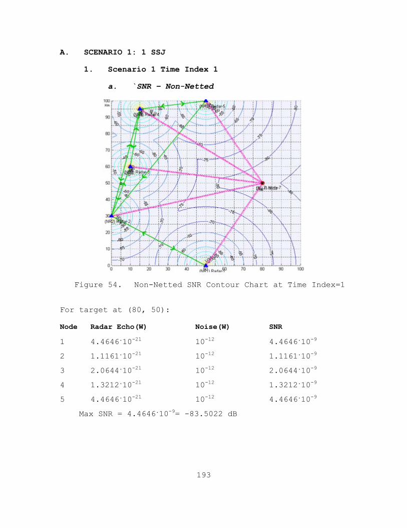
193

A. SCENARIO 1: 1 SSJ

1. Scenario 1 Time Index 1

a. `SNR – Non-Netted

Figure 54. Non-Netted SNR Contour Chart at Time Index=1

For target at (80, 50):

Node Radar Echo(W) Noise(W) SNR

1 4.4646.10-21 10-12 4.4646.10-9

2 1.1161.10-21 10-12 1.1161.10-9

3 2.0644.10-21 10-12 2.0644.10-9

4 1.3212.10-21 10-12 1.3212.10-9

5 4.4646.10-21 10-12 4.4646.10-9

Max SNR = 4.4646.10-9= -83.5022 dB

194

b. `SNR – Netted

Figure 55. Netted SNR Contour Chart at Time Index=1

For target at (80, 50):

Node Radar Echo(W) Noise(W) SNR

1 1.6626.10-21 10-12 1.6626.10-8

2 8.313.10-21 10-12 8.313.10-9

3 1.1306.10-21 10-12 1.1306.10-8

4 9.0446.10-21 10-12 9.0446.10-9

5 1.6626.10-21 10-12 1.6626.10-8

Network disabled

Network enabled

Network improvement

SNR (dB) -83.5022 dB -72.082 dB 11.42 dB

195

c. `JSR – Non-Netted

Figure 56. Non-netted JSR Contour Chart at Time Index=1

For target at (80, 50):

Node Jamming Power(W) Radar Echo (W) JSR

1 1.9075.10-11 4.4646.10-21 4272566008.8821

2 9.5376.10-12 1.1161.10-21 8545132017.7642

3 1.2971.10-11 2.0644.10-21 6283185307.1796

4 1.0377.10-11 1.3212.10-21 7853981633.9745

5 1.9075.10-11 4.4646.10-21 4272566008.8821

Min JSR = 4272566008.8821 = 96.3069 dB

196

d. `JSR – Netted

Figure 57. Netted JSR Contour Chart at Time Index=1

For target at (80, 50):

Node Jamming Power(W) Radar Echo (W) JSR

1 1.9075.10-11 1.6626.10-20 1147305587.7772

2 9.5376.10-11 8.313.10-21 1147305587.7772

3 1.2971.10-11 1.1306.10-20 1147305587.7772

4 1.0377.10-11 9.0446.10-21 1147305587.7772

5 1.9075.10-11 1.6626.10-20 1147305587.7772 Network

disabled Network enabled

Network improvement

JSR (dB) 96.3069 dB 83.6071 12.6998 dB

197

e. `S/(J+N) – Non-Netted

Figure 58. Non-netted SNJR Contour Chart at Time

Index=1

For target at (80, 50):

Node Radar Echo Noise Power Jamming Power SNJR

1 4.4646.10-21 10-12 1.9075.10-11 2.2239.10-10

2 1.1161.10-21 10-12 9.5376.10-12 1.0592.10-10

3 2.0644.10-21 10-12 1.2971.10-11 1.4776.10-10

4 1.3212.10-21 10-12 1.0377.10-11 1.1613.10-10

5 4.4646.10-21 10-12 1.9075.10-11 2.2239.10-10

Max SNJR = 2.2239.10-10= -96.5288 dB

198

f. S/(J+N) – Netted

Figure 59. Netted SNJR Contour Chart at Time Index=1

For target at (80, 50):

Node Radar Echo Noise Power Jamming Power SNJR

1 1.6626.10-20 10-12 1.9075.10-11 8.2819.10-10

2 8.313.10-21 10-12 9.5376.10-10 7.8889.10-10

3 1.1306.10-20 10-12 1.2971.10-11 8.0922.10-10

4 9.0446.10-21 10-12 1.0377.10-11 7.95.10-10

5 1.6626.10-20 10-12 1.9075.10-11 8.2819.10-10

Total SNJR = 4.0495.10-9= -83.926 dB

Network

disabled Network enabled

Network improvement

SNJR (dB) -96.5288 dB -83.926 dB 12.6028 dB

199

2. Scenario 1 Time index 2 (5 LPI Radar + 1 SSJ)

a. SNR Non-Netted

Figure 60. Non-netted SNR Contour Chart at Time Index=2

Analysis of SNR without Network at Time Index = 2

For target at (65, 50):

Node Radar Echo(W) Noise(W) SNR

1 6.9503.10-21 10-12 6.9503.10-9

2 2.4128.10-21 10-12 2.4128.10-9

3 5.2849.10-21 10-12 5.2849.10-9

4 2.5206.10-21 10-12 2.5206.10-9

5 6.9503.10-21 10-12 6.9503.10-9

Max SNR = 6.9503.10-9= -81.58 dB

200

b. SNR Netted

Figure 61. Netted SNR Contour Chart at Time Index=2

For target at (65, 50):

Node Radar Echo(W) Noise(W) SNR

1 2.8242.10-20 10-12 2.8242.10-8

2 1.664.10-20 10-12 1.664.10-8

3 2.4627.10-20 10-12 2.4627.10-8

4 1.7008.10-20 10-12 1.7008.10-8

5 2.8242.10-20 10-12 2.8242.10-8

Total SNR = 1.1476.10-7= -69.4022 dB

Network

disabled Network enabled

Network improvement

SNR (dB) -81.58 dB -69.4022 dB 12.1778 dB

201

c. JSR Non-Netted

Figure 62. Non-netted JSR Contour Chart at Time Index=2

For target at (65, 50):

Node Jamming Power(W) Radar Echo (W) JSR

1 2.38.10-11 6.9503.10-21 3424335992.4129

2 1.4023.10-11 2.4128.10-21 5811946409.1411

3 2.0754.10-11 5.2849.10-21 3926990816.9872

4 1.4333.10-11 2.5206.10-21 5686282702.9975

5 2.38.10-11 6.9503.10-21 3424335992.4129

Min JSR = 3424335992.4129 = 95.3458 dB

202

d. JSR Netted

Figure 63. Netted JSR Contour Chart at Time Index=2

For target at (65, 50):

Node Jamming Power(W) Radar Echo (W) JSR

1 2.38.10-11 2.8242.10-20 842726958.2774

2 1.4023.10-11 1.664.10-20 842726958.2774

3 2.0754.10-11 2.4627.10-20 842726958.2774

4 1.4333.10-11 2.4627.10-20 842726958.2774

5 2.38.10-11 2.8242.10-20 842726958.2774

Total JSR = 168545391.6555 = 82.2672 dB

Network

disabled Network enabled

Network improvement

JSR (dB) 95.3458 dB 82.2672 dB 13.0786 dB

203

e. S/(J+N) Non-Netted

Figure 64. Non-netted SNJR Contour Chart at Time Index=2

For target at (65, 50):

Node Radar Echo Noise Power Jamming Power SNJR

1 6.9503.10-21 10-12 2.38.10-11 2.10-10

2 2.4128.10-21 10-12 1.402310-11 1.6061.10-10

3 5.2849.10-21 10-12 2.0754.10-11 2.4294.10-10

4 2.5206.10-21 10-12 1.4333.10-11 1.6439.10-10

5 6.9503.10-21 10-12 2.38.10-11 2.8025.10-10

Max SNJR = 2.8025.10-9= -95.5245 dB

204

f. S/(J+N) Netted

Figure 65. Netted SNJR Contour Chart at Time Index=2

For target at (65, 50):

Node Radar Echo Noise Power Jamming Power SNJR

1 2.8242.10-20 10-12 2.38.10-11 1.1388.10-9

2 1.664.10-20 10-12 1.4023.10-11 1.1076.10-9

3 2.4627.10-20 10-12 2.0754.10-11 1.1321.10-9

4 1.7008.10-20 10-12 1.4333.10-11 1.1092.10-9

5 2.8242.10-20 10-12 2.38.10-11 1.1388.10-9

Total SNJR = 5.6265.10-9= -82.4976 dB

Network

disabled Network enabled

Network improvement

SNJR (dB) -95.5245 dB -82.4976 dB 13.0269 dB

205

3. Scenario 1 Time index 3 (5 LPI Radar + 1 SSJ)

a. SNR – Non-Netted

Figure 66. Non-netted SNR Contour Chart at Time Index=3

For target at (50, 50):

Node Radar Echo(W) Noise(W) SNR

1 8.2577.10-21 10-12 8.2577.10-9

2 6.1368.10-21 10-12 6.1368.10-9

3 1.7858.10-20 10-12 1.7858.10-8

4 4.8862.10-20 10-12 4.8862.10-8

5 8.2577.10-21 10-12 8.2577.10-9

Max SNR = 1.7858e.10-8= -77.4816 dB

206

b. SNR –Netted

Figure 67. Netted SNR Contour Chart at Time Index=3

For target at (50, 50):

Node Radar Echo(W) Noise(W) SNR

1 4.213.10-20 10-12 4.213.10-8

2 3.6319.10-20 10-12 3.6319.10-8

3 6.1956.10-20 10-12 6.1956.10-8

4 3.2407.10-20 10-12 3.2407.10-8

5 4.213.10-20 10-12 4.213.10-8

Total SNR = 2.1494.10-7= -66.6768 dB

Network

disabled Network enabled

Network improvement

SNR (dB) -77.4816 dB -66.6768 dB 10.8048 dB

207

c. JSR – Non-Netted

Figure 68. Non-netted JSR Contour Chart at Time Index=3

For target at (50, 50):

Node Jamming Power(W) Radar Echo (W) JSR

1 2.5942.10-11 8.2577.10-21 3141592653.5898

2 2.2364.10-11 6.1368.10-21 3644247478.1642

3 3.815.10-11 1.7858.10-20 2136283004.4411

4 1.9956.10-11 4.8862.10-21 4084070449.6667

5 2.5942.10-11 8.2577.10-21 3141592653.5898

Min JSR = 2136283004.4411 = 93.2966 dB

208

d. JSR – Netted

Figure 69. Netted JSR Contour Chart at Time Index=3

For target at (50, 50):

Node Jamming Power(W) Radar Echo (W) JSR

1 2.5942.10-11 4.213.10-20 615770607.2805

2 2.2364.10-11 3.6319.10-20 615770607.2805

3 3.815.10-11 6.1956.10-20 615770607.2805

4 1.9956.10-11 3.2407.10-20 615770607.2805

5 2.5942.10-11 4.213.10-20 615770607.2805

Total JSR = 123154121.4561 = 80.9045 dB

Network disabled

Network enabled

Network improvement

JSR (dB) 93.2966 dB 80.9045 dB 12.3921 dB

209

e. S/(J+N) – Non-Netted

Figure 70. Non-netted SNJR Contour Chart at Time

Index=3

For target at (50, 50):

Node Radar Echo Noise Power Jamming Power SNJR

1 8.2577.10-21 10-12 2.5942.10-11 3.065.10-10

2 6.1368.10-21 10-12 2.2364.10-11 3.8457.10-10

3 1.7858.10-20 10-12 3.815.10-11 4.5615.10-10

4 4.8862.10-21 10-12 1.9956.10-11 2.3317.10-10

5 8.2577.10-21 10-12 2.5942.10-11 3.065.10-10

Max SNJR = 4.5615.10-10= -93.409 dB

210

f. S/(J+N) –Netted

Figure 71. Netted SNJR Contour Chart at Time Index-3

For target at (50, 50):

Node Radar Echo Noise Power Jamming Power SNJR

1 4.213.10-20 10-12 2.5942.10-11 1.5637.10-9

2 3.6319.10-20 10-12 2.2364.10-11 1.0.10-9

3 6.1956.10-20 10-12 3.815.10-11 1.5825.10-9

4 3.2407.10-20 10-12 1.9956.10-11 1.5465.10-9

5 4.213.10-20 10-12 2.5942.10-11 1.5637.10-9

Total SNJR = 7.8109.10-9= -81.073 dB

Network

disabled Network enabled

Network improvement

SNJR (dB) -93.409 dB -81.073 dB 12.336 dB

211

Β. SCENARIO 2: 1 STAND-OFF JAMMER & 1 TARGET

1. Scenario 2 Time Index 1

a. SNR – Non-Netted

Figure 72. Non-netted SNR Contour Chart at Time Index=1

For target at (60, 50):

Node Radar Echo(W) Noise(W) SNR

1 7.6347.10-21 10-12 7.6347.10-9

2 3.2257.10-21 10-12 3.2257.10-9

3 7.6347.10-21 10-12 7.6347.10-9

4 3.1465.10-21 10-12 3.1465.10-9

5 7.6347.10-21 10-12 7.6347.10-9

Max SNR = 7.6347.10-9= -81.1721 dB

212

b. SNR – Netted

Figure 73. Netted SNR Contour Chart at Time Index=1

For the target at (60, 50):

Node Radar Echo (W) Noise(W) SNR

1 3.2768.10-20 10-12 3.2768.10-8

2 2.1299.10-20 10-12 2.1299.10-8

3 3.2768.10-20 10-12 3.2768.10-8

4 2.1036.10-20 10-12 2.1036.10-8

5 3.2768.10-20 10-12 3.2768.10-8

Total SNR = 1.4064.10-7= -68.5189 dB

Network

disabled Network enabled

Network improvement

SNR (dB) -81.1721 dB -68.5189 dB 12.6532 dB

213

c. JSR – Non-Netted

Figure 74. Non-netted JSR Contour Chart at Time Index=1

For target at (60, 50):

Node Jamming Power(W) Radar Echo (W) JSR

1 1.7964.10-11 7.6347.10-21 2352932896.9714

2 9.5095.10-12 3.225.10-21 2948083808.8287

3 1.2951.10-11 7.6347.10-21 1696357488.2551

4 1.021.10-11 3.1465.10-21 3244722585.3052

5 1.796.10-11 7.6347.10-21 2352932896.9714

Min JSR = 1696357488.2551 = 92.2952 dB

214

d. JSR –Netted

Figure 75. Netted JSR Contour Chart at Time Index=1

For target at (60, 50):

Node Jamming Power(W) Radar Echo (W) JSR

1 1.7964.10-11 3.2768.10-20 548216783.1287

2 9.5095.10-12 2.1299.10-20 446473788.393

3 1.2951.10-11 3.2768.10-20 395239339.9933

4 1.021.10-11 2.1036.10-20 485331725.6893

5 1.7964.10-11 3.2768.10-20 548216783.1287

Total JSR = 95433289.1152 = 79.797 dB

Network

disabled Network enabled

Network improvement

JSR (dB) 92.2952 dB 79.797 dB 12.4982 dB

215

e. S/(J+N) – Non-Netted

Figure 76. Non-netted SNJR Contour Chart at Time

Index=1

For target at (60, 50):

Node Radar Echo Noise Power Jamming Power SNJR

1 7.6347.10-21 10-12 1.7964.10-11 4.0259.10-10

2 3.2257.10-21 10-12 9.5095.10-12 3.0693.10-10

3 7.6347.10-21 10-12 1.2951.10-12 5.4724.10-10

4 3.1465.10-21 10-12 1.021.10-11 2.807.10-10

5 7.6347.10-21 10-12 1.7964.10-11 4.0259.10-10

Max SNJR = 5.4724.10-10= -92.6182 dB

216

f. S/(J+N) –Netted

Figure 77. Netted SNJR Contour Chart at Time Index=1

For target at (60, 50):

Node Radar Echo Noise Power Jamming Power SNJR

1 3.2768.10-20 10-12 1.7964.10-11 1.7279.10-9

2 2.1299.10-20 10-12 9.5095.10-12 2.026.10-9

3 3.2768.10-20 10-12 1.2951.10-11 2.3488.10-9

4 2.1036.10-20 10-12 1.021.10-11 1.8766.10-9

5 3.2768.10-20 10-12 1.7964.10-11 1.7279.10-9

Total SNJR = 9.7079.10-9= -80.1288 dB

Network

disabled Network enabled

Network improvement

SNJR (dB) -92.6182 dB -80.1288 dB 12.4894 dB

217

2. Scenario 2 Time Index 2

a. SNR – Non-Netted

Figure 78. Non-netted SNR Contour Chart at Time Index=2

For target at (45, 50):

Node Radar Echo(W) Noise(W) SNR

1 8.095.10-21 10-12 8.095.10-9

2 8.7764.10-21 10-12 8.7764.10-9

3 2.9397.10-20 10-12 2.9397.10-8

4 6.0323.10-21 10-12 6.0323.10-9

5 8.095.10-12 10-12 8.095.10-9

Max SNR = 2.9397.10-8= -75.3169 dB

218

b. SNR –Netted

Figure 79. Netted SNR Contour Chart at Time Index=2

For target at (45, 50):

Node Radar Echo(W) Noise(W) SNR

1 4.7033.10-20 10-12 4.7033.10-8

2 4.8972.10-20 10-12 4.8972.10-8

3 8.9629.10-20 10-12 8.9629.10-8

4 4.0601.10-20 10-12 4.0601.10-8

5 4.7033.10-20 10-12 4.7033.10-8

Total SNR = 2.7327.10-7= -65.6341 dB

Network

disabled Network enabled

Network improvement

SNR (dB) -75.3169 dB -65.6341 dB 9.6828 dB

219

c. JSR – Non-Netted

Figure 80. Non-netted JSR Contour Chart at Time Index=2

For target at (45, 50):

Node Jamming Power(W) Radar Echo (W) JSR

1 2.2003.10-11 8.095.10-21 2718090550.4659

2 1.3922.10-11 8.7764.10-21 1586359166.5851

3 2.0653.10-11 2.9397.10-20 702560415.2673

4 1.3887.10-11 6.0323.10-21 2302130378.0091

5 2.2003.10-11 8.095.10-21 2718090550.4659

Min JSR = 702560415.2673 = 88.4668 dB

220

d. JSR –Netted

Figure 81. Netted JSR Contour Chart at Time Index=2

For target at (45, 50):

Node Jamming Power(W) Radar Echo (W) JSR

1 2.2003.10-11 4.7033.10-20 467817995.0508

2 1.3922.10-11 4.8972.10-20 284291689.5865

3 2.0653.10-11 8.9629.10-20 230431678.4694

4 1.3887.10-11 4.0601.10-20 342041207.0007

5 2.2003.10-11 4.7033.10-20 467817995.0508

Total JSR = 66418763.7848 = 78.2229 dB

Network disabled

Network enabled

Network improvement

JSR (dB) 88.4668 dB 78.2229 dB 10.2439 dB

221

e. S/(J+N) – Non-Netted

Figure 82. Non-netted SNJR Contour Chart at Time

Index=2

For target at (45, 50):

Node Radar Echo Noise Power Jamming Power SNJR

1 8.095.10-21 10-12 2.2003.10-11 3.5191.10-10

2 8.776.10-21 10-12 1.3922.10-11 5.8813.10-10

3 2.9397.10-20 10-12 2.0653.10-11 1.3576.10-9

4 6.0323.10-21 10-12 1.3887.10-11 4.052.10-10

5 8.095.10-21 10-12 2.2003.10-11 3.5191.10-10

Max SNJR = 1.3576e.10-9= -88.6722 dB

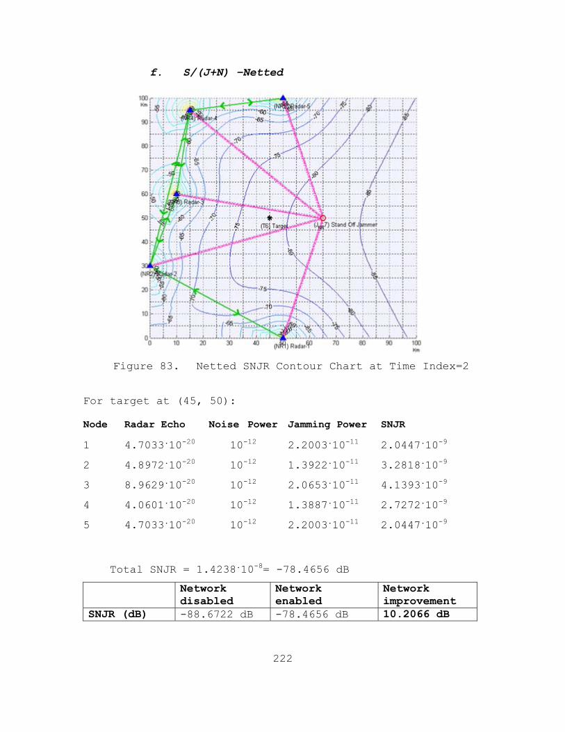
222

f. S/(J+N) –Netted

Figure 83. Netted SNJR Contour Chart at Time Index=2

For target at (45, 50):

Node Radar Echo Noise Power Jamming Power SNJR

1 4.7033.10-20 10-12 2.2003.10-11 2.0447.10-9

2 4.8972.10-20 10-12 1.3922.10-11 3.2818.10-9

3 8.9629.10-20 10-12 2.0653.10-11 4.1393.10-9

4 4.0601.10-20 10-12 1.3887.10-11 2.7272.10-9

5 4.7033.10-20 10-12 2.2003.10-11 2.0447.10-9

Total SNJR = 1.4238.10-8= -78.4656 dB

Network disabled

Network enabled

Network improvement

SNJR (dB) -88.6722 dB -78.4656 dB 10.2066 dB

223

3. Scenario 2 Time Index 3

a. SNR – Non-Netted

Figure 84. Non-netted SNR Contour Chart at Time Index=3

For target at (30, 50):

Node Radar Echo(W) Noise(W) SNR

1 6.1368.10-21 10-12 6.1368.10-9

2 3.0539.10-20 10-12 3.0539.10-8

3 2.0644.10-19 10-12 2.0644.10-7

4 1.0195.10-20 10-12 1.0195.10-8

5 6.1368.10-20 10-12 6.1368.10-9

Max SNR = 2.0644.10-7= -66.852 dB

224

b. SNR –Netted

Figure 85. Netted SNR Contour Chart at Time Index=3

For target at (30, 50):

Node Radar Echo (W) Noise(W) SNR

1 6.9466.10-20 10-12 6.9466.10-8

2 1.5496.10-19 10-12 1.5496.10-7

3 4.0291.10-19 10-12 4.0291.10-7

4 8.9535.10-20 10-12 8.9535.10-8

5 6.9466.10-20 10-12 6.9466.10-8

Total SNR = 7.8634.10-7= -61.0439 dB

Network disabled

Network enabled

Network improvement

SNR (dB) -66.852 dB -61.0439 dB 5.8081dB

225

c. JSR – Non-Netted

Figure 86. Non-netted JSR Contour Chart at Time Index=3

For target at (30, 50):

Node Jamming Power(W) Radar Echo (W) JSR

1 2.4087.10-11 6.1368.10-21 3924974653.5797

2 2.1884.10-11 3.0539.10-20 716607743.2427

3 3.7242.10-11 2.0644.10-19 180398946.8708

4 1.8818.10-11 1.0195.10-20 1845860091.197

5 2.4087.10-11 6.1368.10-21 3924974653.5797

Min JSR = 180398946.8708 = 82.5623 dB

226

d. JSR –Netted

Figure 87. Netted JSR Contour Chart at Time Index=3

For target at (30, 50):

Node Jamming Power(W) Radar Echo (W) JSR

1 2.4087.10-11 6.9466.10-20 346739681.7191

2 2.1884.10-11 1.5496.10-19 141222154.1727

3 3.7242.10-11 4.0291.10-19 92433347.4377

4 1.8818.10-11 8.9535.10-20 210174948.4691

5 2.4087.10-11 6.9466.10-20 346739681.7191

Total JSR = 35179550.0136 = 75.4629 dB

Network disabled

Network enabled

Network improvement

JSR (dB) 82.5623 dB 75.4629 dB 7.0994 dB

227

e. S/(J+N) – Non-Netted

Figure 88. Non-netted SNJR Contour Chart at Time

Index=3

For target at (30, 50):

Node Radar Echo Noise Power Jamming Power SNJR

1 6.1368.10-21 10-12 2.4087.10-11 2.4462.10-10

2 3.0539.10-20 10-12 2.1884.10-11 1.3345.10-9

3 2.0644.10-19 10-12 3.7242.10-11 5.3983.10-9

4 1.0195.10-20 10-12 1.8818.10-11 5.1442.10-10

5 6.1368.10-21 10-12 2.4087.10-11 2.4462.10-10

Max SNJR = 5.3983.10-9= -82.6774 dB

228

f. S/(J+N)– Netted

Figure 89. Netted SNJR Contour Chart at Time Index=3

For target at (30, 50):

Node Radar Echo Noise Power Jamming Power SNJR

1 6.9466.10-20 10-12 2.4087.10-11 2.769.10-9

2 1.5496.10-19 10-12 2.1884.10-11 6.7716.10-9

3 4.0291.10-19 10-12 3.7242.10-11 1.0536.10-8

4 8.9535.10-20 10-12 1.8818.10-11 4.5179.10-9

5 6.9466.10-20 10-12 2.4087.10-11 2.769.10-9

Total SNJR = 2.7363.10-8= -75.6283 dB

Network disabled

Network enabled

Network improvement

SNJR (dB) -82.6774 dB -75.6283 dB 7.049 dB

229

C. SCENARIO 3: 2 STAND IN JAMMERS

1. Scenario 3 Time Index 1

a. SNR – Non-Netted

Figure 90. Non-netted SNR Contour Chart at Time Index=1

For target at (80, 50):

Node Radar Echo(W) Noise(W) SNR

2 1.1161.10-21 10-12 1.1161.10-9

3 2.0644.10-21 10-12 2.0644.10-9

4 1.3212.10-21 10-12 1.3212.10-9

5 4.4646.10-21 10-12 4.4646.10-9

Max SNR = 4.4646.10-9= -83.5022 dB

230

b. SNR – Netted

Figure 91. Netted SNR Contour Chart at Time Index=1

For target at (80, 50):

Node Radar Echo(W) Noise(W) SNR

2 6.0808.10-21 10-12 6.0808.10-9

3 8.2698.10-21 10-12 8.2698.10-9

4 6.6159.10-21 10-12 6.6159.10-9

5 1.2162.10-20 10-12 1.2162.10-9

Total SNR = 3.3128.10-8= -74.7981 dB

Network disabled

Network enabled

Network improvement

SNR (dB) -83.5022 dB -74.7981 dB 8.7041 dB

231

c. JSR – Non-Netted

Figure 92. Non-netted JSR Contour Chart at Time Index=1

For target at (80, 50):

Node Jamming Power(W) Radar Echo (W) JSR

2 6.9891.10-12 1.1161.10-21 6261820912.0461

3 4.6117.10-12 2.0644.10-21 2233896340.3644

4 4.9881.10-12 1.3212.10-21 3775371748.1475

5 7.383.10-12 4.4646.10-21 1653677775.5514

Min JSR = 1653677775.5514 = 92.1845 dB

232

d. JSR –Netted

Figure 93. Netted JSR Contour Chart at Time Index=1

For target at (80, 50):

Node Jamming Power(W) Radar Echo (W) JSR

2 6.9891.10-12 6.0808.10-21 1149379756.2493

3 4.6117.10-12 8.2698.10-21 557654005.671

4 4.9881.10-12 6.6159.10-21 753965576.7226

5 7.383.10-12 1.2162.10-20 607077010.1143

Total JSR = 177405020.9081 = 82.4897 dB

Network disabled

Network enabled

Network improvement

JSR (dB) 92.1845 dB 82.4897 dB 9.6948 dB

233

e. S/(J+N) – Non-Netted

Figure 94. Non-netted SNJR Contour Chart at Time

Index=1

For target at (80, 50):

Node Radar Echo Noise Power Jamming Power SNJR

2 1.1161.10-21 10-12 6.9891.10-12 1.3971.10-10

3 2.0644.10-21 10-12 4.6117.10-12 3.6788.10-10

4 1.3212.10-21 10-12 4.9881.10-12 2.2064.10-10

5 4.4646.10-21 10-12 7.383.10-12 5.3258.10-10

Max SNJR = 5.3258.10-10= -92.7362 dB

234

f. S/(J+N)- Netted

Figure 95. Netted SNJR Contour Chart at Time Index=1

For target at (80, 50):

Node Radar Echo Noise Power Jamming Power SNJR

2 6.0808.10-21 10-12 6.9891.10-12 7.6113.10-10

3 8.2698.10-21 10-12 4.6117.10-12 1.4737.10-9

4 6.6159.10-21 10-12 4.9881.10-12 1.1048.10-9

5 1.2162.10-20 10-12 7.383.10-12 1.4507.10-9

Total SNJR = 4.7904.10-9= -83.1963 dB

Network disabled

Network enabled

Network improvement

SNJR (dB) -92.7362 dB -83.1963 dB 9.5399 dB

235

2. Scenario 3 Time Index 2

a. SNR – Non-Netted

Figure 96. Non-netted SNR Contour Chart at Time Index=2

For target at (65, 55):

Node Radar Echo(W) Noise(W) SNR

2 2.1941.10-21 10-12 2.1941.10-9

3 5.548.10-21 10-12 5.548.10-9

4 3.0702.10-21 10-12 3.0702.10-9

5 1.0195.10-20 10-12 1.0195.10-8

Max SNR = 1.0195.10-8= -79.9163 dB

236

b. SNR – Netted

Figure 97. Netted SNR Contour Chart at Time Index=2

For target at (65, 55):

Node Radar Echo(W) Noise(W) SNR

2 1.3008.10-20 10-12 1.3008.10-8

3 2.0685.10-20 10-12 2.0685.10-8

4 1.5387.10-20 10-12 1.5387.10-8

5 2.8039.10-20 10-12 2.8039.10-8

Total SNR = 7.712.10-8= -71.1283 dB

Network disabled

Network enabled

Network improvement

SNR (dB) -79.9163 dB -71.1283 dB 8.788 dB

237

c. JSR – Non-Netted

Figure 98. Non-netted JSR Contour Chart at Time Index=2

For target at (65, 55):

Node Jamming Power(W) Radar Echo (W) JSR

2 8.9448.10-12 2.1941.10-21 4076774915.7844

3 6.9522.10-12 5.548.10-21 1253087303.8055

4 7.5613.10-12 3.0702.10-21 2462799115.4328

5 9.172.10-12 1.0195.10-20 899683794.9771

Min JSR = 899683794.9771 = 89.5409 dB

238

d. JSR – Netted

Figure 99. Netted JSR Contour Chart at Time Index=2

For target at (65, 55):

Node Jamming Power(W) Radar Echo (W) JSR

2 8.9448.10-12 1.3008.10-20 687640094.5942

3 6.9522.10-12 2.0685.10-20 336099360.6127

4 7.5613.10-12 1.5387.10-20 491395673.1209

5 9.172.10-12 2.8039.10-20 327109815.3063

Total JSR = 105023736.6453 = 80.2129 dB

Network disabled

Network enabled

Network improvement

JSR (dB) 89.5409 dB 80.2129 dB 9.328 dB

239

e. S/(J+N) – Non-Netted

Figure 100. Non-netted SNJR Contour Chart at Time

Index=2

For target at (65, 55):

Node Radar Echo Noise Power Jamming Power SNJR

2 2.1941.10-21 10-12 8.9448.10-12 2.2063.10-10

3 5.548.10-21 10-12 6.9522.10-12 6.9768.10-10

4 3.0702.10-21 10-12 7.5613.10-12 3.5861.10-10

5 1.0195.10-20 10-12 9.172.10-12 1.0022.10-9

Max SNJR = 1.0022.10-9= -89.9903 dB

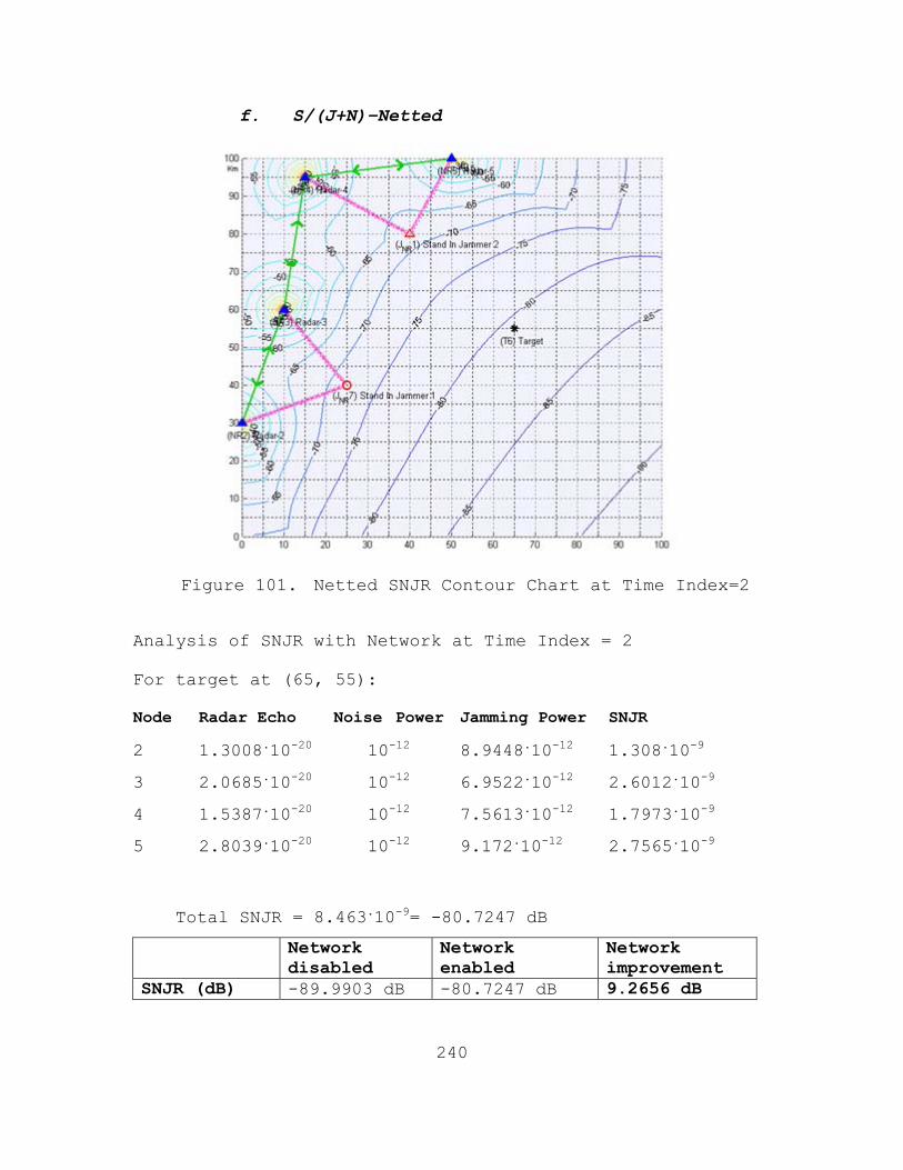
240

f. S/(J+N)–Netted

Figure 101. Netted SNJR Contour Chart at Time Index=2

Analysis of SNJR with Network at Time Index = 2

For target at (65, 55):

Node Radar Echo Noise Power Jamming Power SNJR

2 1.3008.10-20 10-12 8.9448.10-12 1.308.10-9

3 2.0685.10-20 10-12 6.9522.10-12 2.6012.10-9

4 1.5387.10-20 10-12 7.5613.10-12 1.7973.10-9

5 2.8039.10-20 10-12 9.172.10-12 2.7565.10-9

Total SNJR = 8.463.10-9= -80.7247 dB

Network disabled

Network enabled

Network improvement

SNJR (dB) -89.9903 dB -80.7247 dB 9.2656 dB

241

3. Scenario 3 Time Index 3

a. SNR – Non-Netted

Figure 102. Non-netted SNR Contour Chart at Time Index=3

For target at (50, 60):

Node Radar Echo(W) Noise(W) SNR

2 4.4646.10-21 10-12 4.4646.10-9

3 2.016.10-21 10-12 2.016.10-8

4 8.5982.10-21 10-12 8.5982.10-9

5 2.016.10-20 10-12 2.016.10-8

Max SNR = 2.016.10-8= -76.955 dB

242

b. SNR –Netted

Figure 103. Netted SNR Contour Chart at Time Index=3

For target at (50, 60):

Node Radar Echo(W) Noise(W) SNR

2 2.9635.10-20 10-12 2.9635.10-8

3 6.2974.10-20 10-12 6.2974.10-8

4 4.1126.10-20 10-12 4.1126.10-8

5 6.2974.10-20 10-12 6.2974.10-8

Total SNR = 1.9671.10-7= -67.0618 dB

Network disabled

Network enabled

Network improvement

SNR (dB) -76.955 dB -67.0618 dB 9.8932 dB

243

c. JSR – Non-Netted

Figure 104. Non-netted JSR Contour Chart at Time Index=3

For target at (50, 60):

Node Jamming Power(W) Radar Echo (W) JSR

2 1.2933.10-11 4.4646.10-21 2896787150.5551

3 5.8009.10-12 2.016.10-20 287736411.3834

4 1.2305.10-11 8.5982.10-21 1431176785.5706

5 1.0191.10-11 2.016.10-20 505501347.6305

Min JSR = 287736411.3834 = 84.5899 dB

244

d. JSR –Netted

Figure 105. Netted JSR Contour Chart at Time Index=3

For target at (50, 60):

Node Jamming Power(W) Radar Echo (W) JSR

2 1.2933.10-11 2.9635.10-20 436410669.8761

3 5.8009.10-12 6.2974.10-20 92115461.446

4 1.2305.10-11 4.1126.10-20 299216053.5551

5 1.0191.10-11 6.2974.10-20 161830369.937

Total JSR = 44113617.6938 = 76.4457 dB

Network disabled

Network enabled

Network improvement

JSR (dB) 84.5899 dB 76.4457 dB 8.1442 dB

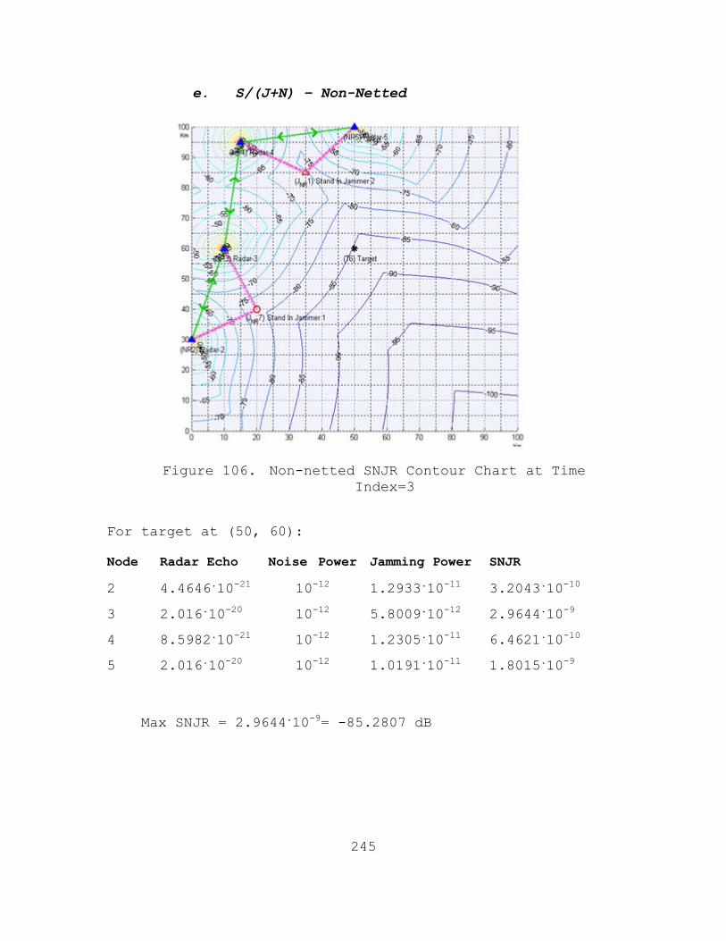
245

e. S/(J+N) – Non-Netted

Figure 106. Non-netted SNJR Contour Chart at Time

Index=3

For target at (50, 60):

Node Radar Echo Noise Power Jamming Power SNJR

2 4.4646.10-21 10-12 1.2933.10-11 3.2043.10-10

3 2.016.10-20 10-12 5.8009.10-12 2.9644.10-9

4 8.5982.10-21 10-12 1.2305.10-11 6.4621.10-10

5 2.016.10-20 10-12 1.0191.10-11 1.8015.10-9

Max SNJR = 2.9644.10-9= -85.2807 dB

246

f. S/(J+N) –Netted

Figure 107. Netted SNJR Contour Chart at Time Index=3

For target at (50, 60):

Node Radar Echo Noise Power Jamming Power SNJR

2 2.9635.10-20 10-12 1.2933.10-11 2.127.10-9

3 6.2974.10-20 10-12 5.8009.10-12 9.2597.10-9

4 4.1126.10-20 10-12 1.2305.10-11 3.0909.10-9

5 6.2974.10-20 10-12 1.0191.10-11 5.6271.10-9

Total SNJR = 2.0105.10-8= -76.967 dB

Network disabled

Network enabled

Network improvement

SNJR (dB) -85.2807 dB -76.967 dB 8.3137 dB

247

Table 15 summarizes the results of the

simulation.

Scenarios

Max SNJR

(Non-Netted)or

Total SNJR (Netted)

RiSNR TARGET

DETECTION

Non-Netted -92.5288 dB -92.65 dB YES

Step 1

Netted -83.9260 dB -92.65 dB YES

Non-Netted -95.5245 dB -92.65 dB NO

Step 2

Netted -82.4976 dB -92.65 dB YES

Non-Netted -93.4090 dB -92.65 dB NO

Scenario 1

Step 3

Netted -81.0730 dB -92.65 dB YES

Non-Netted -92.6182 dB -92.65 dB YES

Step 1

Netted -80.1218 dB -92.65 dB YES

Non-Netted -88.6722 dB -92.65 dB YES

Step 2

Netted -78.4656 dB -92.65 dB YES

Non-Netted -82.6774 dB -92.65 dB YES

Scenario 2

Step 3

Netted -75.6283 dB -92.65 dB YES

Non-Netted -92.7302 dB -92.65 dB NO

Step 1

Netted -83.1963 dB -92.65 dB YES

Non-Netted -89.9903 dB -92.65 dB YES

Step 2

Netted -80.7247 dB -92.65 dB YES

Non-Netted -85.2807 dB -92.65 dB YES

Scenario 3

Step 3

Netted -76.9670 dB -92.65 dB YES

Table 15. Summary of Simulation Results

248

Having all other parameters constant (radar

positions, radar characteristics, target RCS, target

movement, etc.) and changing only the type of operation

(netted versus non-netted mode of operation), the preceding

results are heavily dependent on the jammer characteristics

(jammer ERP, jammer capability), the jammer’s distance from

the radar nodes and the Target’s distance from the radar

nodes.

A careful study of Table 15 indicates that the

netted configuration has no problem detecting the target in

any scenario and at any time step. In fact, the netted

configuration has a significant advantage over the non-

netted one, not only in terms of higher SNR, JSR and SNJR

values, but also by achieving 100% detection probability.

For the analysis of the non-netted configuration

we examine each scenario separately:

• Non-Netted Scenario 1

Scenario 1 is a pure Self Screening Jamming (SSJ)

scenario where the target and jammer coincide. In this

specific scenario, the on-board jammer has a moderate ERP

(10 Watts) and a good (0.75) jamming capability. In time

steps 2 and 3 of the non-netted configuration, the jamming

was effective and there was no detection by the radar grid.

This can be explained by two factors: (1) the jammer is on-

board the target so there is no additional free space loss-

-as, for instance in the case of Stand-off Jamming (SOJ);

and (2) the jammer has good ERP jamming capabilities.

If we examine more closely time step 1 of

scenario 1 we’ll see that even though there is target

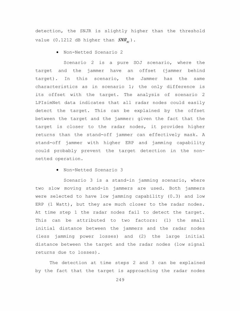
249

detection, the SNJR is slightly higher than the threshold

value (0.1212 dB higher than RiSNR ).

• Non-Netted Scenario 2

Scenario 2 is a pure SOJ scenario, where the

target and the jammer have an offset (jammer behind

target). In this scenario, the Jammer has the same

characteristics as in scenario 1; the only difference is

its offset with the target. The analysis of scenario 2

LPIsimNet data indicates that all radar nodes could easily

detect the target. This can be explained by the offset

between the target and the jammer: given the fact that the

target is closer to the radar nodes, it provides higher

returns than the stand-off jammer can effectively mask. A

stand-off jammer with higher ERP and jamming capability

could probably prevent the target detection in the non-

netted operation.

• Non-Netted Scenario 3

Scenario 3 is a stand-in jamming scenario, where

two slow moving stand-in jammers are used. Both jammers

were selected to have low jamming capability (0.3) and low

ERP (1 Watt), but they are much closer to the radar nodes.

At time step 1 the radar nodes fail to detect the target.

This can be attributed to two factors: (1) the small

initial distance between the jammers and the radar nodes

(less jamming power losses) and (2) the large initial

distance between the target and the radar nodes (low signal

returns due to losses).

The detection at time steps 2 and 3 can be explained

by the fact that the target is approaching the radar nodes

250

faster than the stand-in jammers do; this causes the

target’s returns into the radar nodes to increase faster

than the jamming power does. Two stand-in jammers with

higher ERP and/or jamming capability or at closer distance

to the radar, or moving at higher speed could probably

prevent the target detection in the non-netted operation.

In all scenarios the netted version has an

additional effect on SNJR that varies from +7.049 dB

(minimum improvement) to +13.0269 dB (maximum improvement)

which in layman terms--keeping the noise power the same in

all cases)--means that jamming power into the radar

receiver has to be from 5.069 to 20.077 times higher in

order to mask the target.

This advantage of the netted configuration ,set

against the non-netted configuration is mathematically

explained in the work of Hume and Baker, and Papoutsis,

Barker and Griffiths (Hume and Barker, 2001; Papoutsis, et.

al, 2003): By netting several radars, and assuming that all

radars are transmitting and are capable of receiving apart

from their own echo the echoes from the other radars and

that there is network synchronization, we get an increase

in SNR by the square of the number of the total number of

radar systems comprising the network. The formula for the

SNR of the netted radar system is:

( )( ) ( )2 2

1 1 8.1

44

n nr e

µ ν νµ

ERP µ A νSNRπR Noise νπR= =

=∑ ∑

Where:

rERP µ : Effective radiated power of radar µ .

251

eA ν : Effective antenna area of radar ν .

Noise ν : Noise power of radar ν .

µR : Range from radar µ to target.

νR : Range from target to radar ν .

252

THIS PAGE INTENTIONALLY LEFT BLANK

253

IX. CONCLUSIONS

This thesis provides a comprehensive view of two major

elements in Electronic Warfare: LPI assets and network

configurations. With the existing scholarly efforts dealing

individually with either of these two elements being not

only extensive but also constantly updated, we attempted to

fill the literature gap and provide a more comprehensive

work discussing and linking both areas within the same

work.39

The simulations to achieve our data were performed

with MATLAB-based software, using a standardized data set

(LPIsimNet). Utilizing this tool, it was possible to

numerically prove that the netted LPI IADS is less

vulnerable to jamming attack than a non-netted LPI IADS.

Although the results are not surprising (we expected a

netted LPI IADS to be less susceptible to jamming than a

non-netted one), the accuracy of the output data is

affected by several factors pertaining to the limitations

of the software used.

Running the LPIsimNet, we noted that the absence of a

parameter precisely describing the ease of flow between the

assets is among the most notable factors affecting the

accuracy of the output data. To account for this parameter,

LPIsimNet requires a value for the “capability of

39 The 2008 paper of Chen and Pace presents a basic framework for

simulation of network enabled radar systems, but, apart from being limited in breadth, its scope is limited in the evaluation of the jamming effect in general radar topology. Y. Q. Chen and Phillip E. Pace, “Simulation of Information Metrics to Assess the Value of Networking in A General Battlespace Topology,” in Proc. of the IEEE International Conf. on System of Systems Engineering (IEEE, June 2008).

254

information” of each of the nodes utilized;40 however, this

parameter lacks a mathematical formula for its precise

calculation. In the absence of such a formula, and in order

to reflect the reduced capabilities of nodes 2 and 3 in our

simulation scenario, we arbitrarily assumed that their

“capability of information” was 0.7 instead of 1

(maximum).In order to enhance the computation accuracy and

provide real operational results, the extraction of a

mathematical formula computing precisely the “capability of

information” is recommended for future work.

A second parameter that affects the output data of the

simulation pertains to the RCS, as LPIsimNet assumes that

the RCS of the target/jammer remains the same throughout

its approach towards the radar grid. Such an arbitrary

assumption generates extra inaccuracies, as the RCS is

affected by several parameters.41As detailed computation of

the netted vs. non-netted configuration performance was

outside the scope of this paper, no alteration of the

existing program code was attempted. In this context, the

introduction of a real time RCS computational tool--within

the LPIsimNet code if feasible-is highly recommended as a

means to enhance the realism of the scenarios and provide

more realistic results for existing assets.

Our work asserts that networks of radar systems

present many advantages compared to the traditional concept

40 The min value for the “capability of information” input is 0, and

the max value is 1. 41 Among the major factors are: the material of which the target is

made; the absolute size of the target; the relative size of the target (that is, in relation to the wavelength of the illuminating radar); the incident angle, which depends upon the shape of the target and its orientation to the radar source; the reflected angle; the strength of the radar emitter; and the distance between the radar and the emitter.

255

of autonomous radar assets. Simple independent networks

offer a subset of these advantages and are a logical first

step. More sophisticated coherent networks offer the

ultimate in performance. However, further research is

required to truly establish the merits of this mode of

operation and to overcome the technical challenges it

presents.

256

THIS PAGE INTENTIONALLY LEFT BLANK

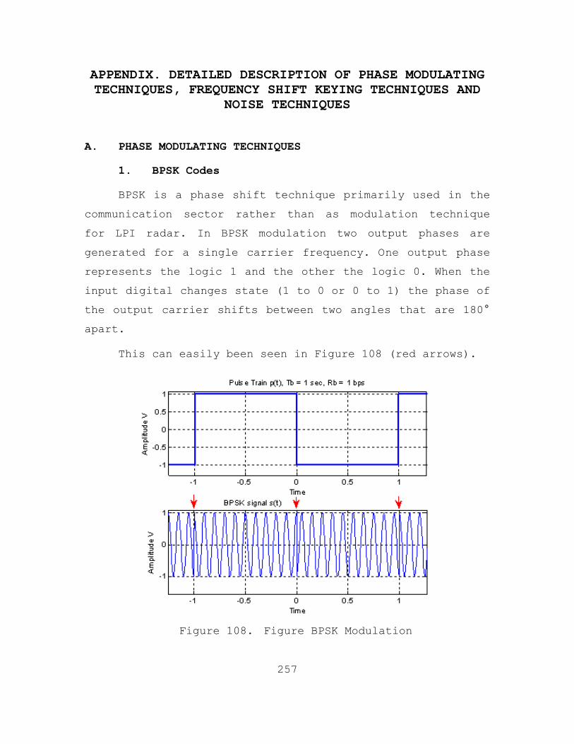
257

APPENDIX. DETAILED DESCRIPTION OF PHASE MODULATING TECHNIQUES, FREQUENCY SHIFT KEYING TECHNIQUES AND

NOISE TECHNIQUES

A. PHASE MODULATING TECHNIQUES

1. BPSK Codes

BPSK is a phase shift technique primarily used in the

communication sector rather than as modulation technique

for LPI radar. In BPSK modulation two output phases are

generated for a single carrier frequency. One output phase

represents the logic 1 and the other the logic 0. When the

input digital changes state (1 to 0 or 0 to 1) the phase of

the output carrier shifts between two angles that are 180°

apart.

This can easily been seen in Figure 108 (red arrows).

Figure 108. Figure BPSK Modulation

258

The typical BPSK codes used for BPSK modulation are

the Barker Codes. The binary Barker sequences are finite-

length discrete time sequences with constant magnitude and

a phase of either = 0kφ or =kφ π . The only known lengths

of Barker sequences are = 2,3,4,5,7,11,13cN . The nine different

Barker codes along with their respective peak sidelobe

level (PSL) with respect to main lobe level can be seen in

Table 16 below(Pace 2009, 128):

Code Length

Code Elements PSL (dB)

2 - + , + - -6.03 + + - -9.54 + + - +, + + + - -12.05 + + + - + -14.07 + + + - - + - -16.911 + + + - - - + - - + - -20.813 + + + + + - - + + - + - + -22.3

Table 16. Barker Codes

Another BPSK technique is to use Compound Barker

Codes, which creates a sequence by implementing a Barker

code within a Barker code. In this way we can create a

larger sequence code that has a sequence of:

= = 2 A.1compoundc c c cN N N N

A compound 4 Barker code is presented in Table 17.

Primary code

+ + - +

Embedded Code

+ + - + + + - + + + - + + + - +

Final Code

+ + - + + + - + - - + - + + - +

Table 17. Compound Barker Code for 4cN =

259

In Figure 109, by using the MATLAB LPIT TOOLBOX, we

see an example of a Barker code BPSK wave modulated by a 7

code length Barker code and added white Gaussian noise,

with parameters: =1cf kHz , =7sf kHz , = 0SNR dB , =7cN .

Figure 109. BPSK Signal Modulated by Barker Code (length

7)

Compound Barker codes give a very large length of code

sequences that can improve range resolution and also give a

higher compression gain, but their peak sidelobes are not

proportionally decreased (due to this higher compression

gain)(Pace 2009, 128).

There are three major disadvantages with the use of

Barker codes.

260

• There are only few (9) known Barker code

sequences that have a very limited length and thus limit

the range resolution.

• Even in the case of compound Barker codes that

can have very large sequences of codes their peak sidelobes

are not proportionally decreased due this high compression

gain.

• They are very sensitive to Doppler shifts. The

Doppler shift of the return waveform can compress the

waveform within the filter such that the matched filter

gives incorrect results.

2. Polyphase Codes

Polyphase sequences are finite length, discrete time

complex sequences with constant magnitude and variable

phase kϕ . Polyphase coding is the phase modulation of the CW

carrier by a polyphase sequence that has a number of

discrete phases (Pace 2009, 133).

Various codes satisfy the above criteria; Polyphase

Barker codes, Frank, P1, P2, P3 and P4 codes. Polyphase

codes derive from approximating a stepped (in the case of

Frank, P1 and P2) or linear (in the case of P3 and P4)

frequency modulation waveform, where the phase steps vary

as needed to approximate the underlying waveform, but the

time spent at any given phase state is constant. A short

description of the polyphase codes follows.

a. Polyphase Barker Codes

Polyphase sequences that satisfy the Barker

criteria are under investigation in order to try finding

261

longer sequences. Various algorithms have been used and/or

developed in order to develop longer polyphase Barker

codes. Currently ≤63cN codes have been discovered (Pace,

2009, 134).

b. Frank Code

Frank code, developed by R.L. Frank in 1963, has

been used successfully in LPI radar. The Frank code is

derived from a step approximation to a linear frequency

modulation waveform using M frequency steps and M samples

per frequency. Its length (or processing gain) is = 2cN M .

The phase of the Frank code is given by the following

formula (Pace 2009, 143):

= − −,2 1 1 A.2i jπφ i jM

Where:

,i jφ : Phase of the thi sample of the thj frequency

=1,2,...,i M

=1,2,...,j M

In Figures 110 and 111, by using the MATLAB LPIT

TOOLBOX, we see a Frank code modulated CW wave, signal

phase and code phase diagrams, with parameters: =1cf kHz ,

=7sf kHz , = 0SNR dB and =16M .

262

Figure 110. Frank Code Phase

Figure 111. Signal Phase (Modulated by Frank Code)

263

c. P1 Code

P1 code is similar to the Frank code. It is also

derived from a step approximation to a linear frequency

modulation waveform using M frequency steps and M samples

per frequency. Its length (or processing gain) is = 2cN M .

The phase of the P1 code is given by the following formula

(Pace 2009, 148):

− ⎡ ⎤ ⎡ ⎤= − − − + −⎣ ⎦ ⎣ ⎦, 2 1 1 1 A.3i jπφ M j j M iM

Where:

,i jφ : Phase of the thi sample of the thj frequency

=1,2,3,....M

=1,2,...,i M

=1,2,...,j M

In Figures 112 and 113, by using the MATLAB LPIT

TOOLBOX, we see a P1 code modulated CW wave, signal phase

and code phase diagrams, with parameters: =1cf kHz , =7sf kHz , = 0SNR dB and =16M .

264

Figure 112. P1 Code Phase

Figure 113. Signal Phase (Modulated by P1 Code)

265

d. P2 Code

P2 code is similar to P1 code, but should be

even and the starting phases are different than with P1

code. It is also derived from a step approximation to a

linear frequency modulation waveform using M frequency

steps and M samples per frequency. Its length (or

processing gain) is = 2cN M . The phase of the P2 code is

given by the following formula (Pace 2009, 152).

−= − − − −, 2 1 2 1 A.42i j

πφ i M j MM

Where:

,i jφ : Phase of the thi sample of the thj frequency

=2,4,6,....M

=1,2,...,i M

=1,2,...,j M

In Figures 114 and 115, by using the MATLAB LPIT

TOOLBOX, we see a P2 code modulated CW wave, signal phase

and code phase diagrams, with parameters: =1cf kHz , =7sf kHz , = 0SNR dB and =16M .

266

Figure 114. P2 Code Phase

Figure 115. Signal Phase (Modulated by P2 Code)

267

e. P3 Code

P3 code is derived by converting a linear

frequency modulation waveform to baseband. That is done by

using a synchronous oscillator on one end of the frequency

sweep and sampling the in-phase (I) and quadrature (Q)

channels at the Nyquist rate (the sampling frequency ≤2sf W

where W is the highest frequency of the signal) resulting

in a single sideband detection. The phase of the P3 code is

given by the following formula (Pace 2009, 152):

= − 21 A.5ic

πφ iN

Where:

iφ : Phase of the thi sample

cN : Compression ratio

=1,2,..., ci N

In Figures 116 and 117, by using the MATLAB LPIT

TOOLBOX, we show a P3 code modulated CW wave, signal phase

and code phase diagrams, with parameters: =1cf kHz , =7sf kHz , = 0SNR dB and =32M .

268

Figure 116. P3 Code Phase

Figure 117. Signal Phase (Modulated by P3 Code)

269

f. P4 Code

P4 code is similar to P3 code, but the oscillator

that does the sampling of the in-phase (I) and quadrature

(Q) channels has an offset between I and Q channels,

resulting in coherent double sideband detection. Again, the

sampling is done at the Nyquist rate (the sampling

frequency ≤2sf W where W is the highest of the signal). The

phase of the P4 code is given by the following formula

(Pace 2009, 157).

−= − −

21 1 A.6ic

π iφ π iN

Where:

iφ : Phase of the thi sample

cN : Compression ratio

=1,2,..., ci N

In Figures 118 and 119, by using the MATLAB LPIT

TOOLBOX, we show a P4 code modulated CW wave, signal phase

and code phase diagrams, with parameters: =1cf kHz , =7sf kHz , = 0SNR dB and =32M .

270

Figure 118. P4 Code Phase

Figure 119. Signal Phase (Modulated by P4 Code)

271

3. Polytime Codes

Polyphase codes derive from approximating a stepped

(in the case of Frank, P1 and P2) or linear (in the case of

P3 and P4) frequency modulation waveform, where the phase

steps vary as needed to approximate the underlying

waveform, but the time spent at any given phase state is

constant. For polytime codes there is different process;

the underlying waveform is quantized into a user-selected

number of phase states. So for polytime codes the phase

states are fixed, but there are varying time periods at

each phase state (Pace 2009, 163). There are four polytime

sequences as follows.

a. T1(n)

T1(n) is generated from a stepped frequency

waveform where n is the number of phase states used to

approximate the underlying waveform. The formula of the

phase of the polytime sequence T1(n) is as follows(Pace

2009, 163).

⎧ ⎫⎡ ⎤⎪ ⎪= −⎨ ⎬⎢ ⎥⎪ ⎪⎣ ⎦⎩ ⎭

12mod ,2 A.7Tπ jnφ t INT kt jT πn T

Where:

n : Number of phase states in the code sequence

k : Number of segments in the T1 code sequence

T : Overall code duration

= −0,1,2,..., 1j k : Segment number in the stepped frequency

waveform

272

In Figures 120 and 121, by using the MATLAB LPIT

TOOLBOX, a T1(2) code modulated CW wave, stepped frequency

phase shift and time domain waveform, with parameters:

=1cf kHz , =7sf kHz , = 0SNR dB , = 2n , = 0.016secT , =Δ 250F Hz and = 4k are depicted.

Figure 120. T1(2) Stepped Frequency Phase

Figure 121. T1(2) Modulated Signal Time Domain Waveform

273

b. T2(n)

T2(n) is generated from a stepped frequency

waveform where n is the number of phase states used to

approximate the underlying waveform. The formula of the

phase of the polytime sequence T2(n) is as follows(Pace

2009, 165).

⎧ ⎫⎡ ⎤⎛ ⎞− +⎪ ⎪= −⎨ ⎬⎢ ⎥⎜ ⎟⎝ ⎠⎪ ⎪⎣ ⎦⎩ ⎭

22 2 1mod ,2 A.82Tπ j k nφ t INT kt jT πn T

Where:

n : Number of phase states in the code sequence

k : Number of segments in the T1 code sequence

T : Overall code duration

= −0,1,2,..., 1j k : Segment number in the stepped frequency

waveform

In Figures 122 and 123, by using the MATLAB LPIT

TOOLBOX, a T2(2) code modulated CW wave, stepped frequency

phase shift and time domain waveform, with parameters:

=1cf kHz , =7sf kHz , = 0SNR dB , = 2n , = 0.016secT , =Δ 250F Hz and = 4k are depicted.

274

Figure 122. T2(2) Stepped Frequency Phase

Figure 123. T2(2) Modulated Signal Time Domain Waveform

275

c. T3(n)

T3(n) is generated from approximations of a

linear frequency model, where n is the number of phase

states used to approximate the underlying waveform. The

formula of the phase of the polytime sequence T3(n) is the

following (Pace, 2009, 169):

⎧ ⎫⎡ ⎤⎪ ⎪= ⎨ ⎬⎢ ⎥⎪ ⎪⎣ ⎦⎩ ⎭

2

32 Δmod ,2 A.92T

m

π n Ftφ t INT πn t

Where:

n : Number of phase states in the code sequence

ΔF : Modulation bandwidth

mt : Modulation period

In Figures 124 and 125, by using the MATLAB LPIT

TOOLBOX, we see a T3(2) code modulated CW wave, stepped

frequency phase shift and time domain waveform, with

parameters =1cf kHz , =7sf kHz , = 0SNR dB , = 2n and =Δ 250F Hz .

276

Figure 124. T3(2) Stepped Frequency Phase

Figure 125. T3(2) Modulated Signal Time Domain Waveform

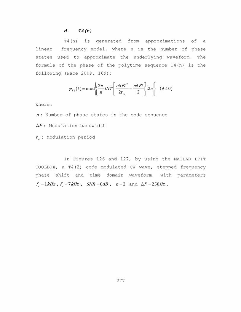
277

d. T4(n)

T4(n) is generated from approximations of a

linear frequency model, where n is the number of phase

states used to approximate the underlying waveform. The

formula of the phase of the polytime sequence T4(n) is the

following (Pace 2009, 169):

⎧ ⎫⎡ ⎤⎪ ⎪= −⎨ ⎬⎢ ⎥⎪ ⎪⎣ ⎦⎩ ⎭

2

42 Δ Δmod ,2 A.102 2T

m

π n Ft n Ftφ t INT πn t

Where:

n : Number of phase states in the code sequence

ΔF : Modulation bandwidth

mt : Modulation period

In Figures 126 and 127, by using the MATLAB LPIT

TOOLBOX, a T4(2) code modulated CW wave, stepped frequency

phase shift and time domain waveform, with parameters

=1cf kHz , =7sf kHz , = 0SNR dB , = 2n and =Δ 250F Hz .

278

Figure 126. T4(2) Stepped Frequency Phase

Figure 127. T4(2) Modulated Signal Time Domain Waveform

279

B. FREQUENCY SHIFT KEYING (FSK) TECHNIQUES

1. Costas Codes

Costas codes were developed by J.P. Costas. They are a

sequence of frequencies that provide unambiguous range and

Doppler measurements while minimizing the cross talk

between frequencies. They have peak sidelobes that are down

from the mainlobe by a factor of 1/ FN ( FN is the number of

contiguous frequencies within a band B and each frequency lasts pt seconds)(Pace 2009, 191).

There are various methods to construct a Costas

sequence, such as the Welch construction, the Lempel

construction, the Golomb construction, Taylor’s 4T

construction, and the 4G and 5G constructions. An

exhaustive search to find all x n n Costas arrays (which has currently been completed for ≤26n ), as well as others being

developed (Golomb 2006), is not within the scope of the

present thesis to enumerate.

Instead, by using the MATLAB LPIT TOOLBOX, for the

known Costas sequence 2, 4, 8, 5, 10, 9, 7, 3, 6, 1 kHz , for

= 0SNR dB , = 0.1secpt , =15sf kHz we present in Figures 128 and 129 the PSD plots of the I channel with and without noise

(AWGN).

280

Figure 128. I Channel PSD with Noise SNR=0dB

Figure 129. I Channel PSD with No Noise

281

2. Hybrid FSK/PSK Technique

The proposed technique(Pace 2009, 195) combines an FSK

technique (Frequency Hoping using Costas sequences) with a

PSK technique. The FH LPI radar waveform has FN frequencies

within a bandwidth B . Every frequency lasts pt seconds in

duration. The proposed hybrid technique subdivided each

subperiod pt (that one of the FN frequencies is transmitted)

into BN phase slots, each with duration bt . The

mathematical relationships of the proposed scheme are:

= = A.11B p b BT t t N

= A.12T F BN N N

= = A.13p F b B FT t N t N N

Where:

pt : Duration of each frequency

bt : Duration of each phase slot

FN : Number of frequencies

BN : Number of phase slots

T : Total code (FSK/PSK) period

BT : PSK code period

The formula of the complex envelope of the transmitted

CW FSK/PSK wave is the following (Pace 2009, 196):

+= 2 A.23j kj πf t φs t Ae

282

Where:

kφ : One of the PSK codes

jf : One of the FSK frequencies

In Figures 130 and 131, by using the MATLAB LPIT

TOOLBOX, we present the plot of PSD of a FSK (Costas) CW

LPI waveform and an FSK(same Costas)/PSK(Barker) CW LPI

waveform with the parameters: Barker code length 5, Costas

sequence 3, 2, 6, 4, 5, 1 kHz , =15sf kHz , = 0SNR dB and = 0.006secpt .

Figure 130. FSK (Costas Only) PSD

283

Figure 131. Hybrid FSK (Costas)/PSK (Barker) PSD

3. Matched FSK/PSK Technique

This type of technique generates FSK/PSK signals

optimally matched to an arbitrary target’s spectral

response. Radar uses FSK/PSK signal but instead of

selecting the frequency from a Costas sequence (as in the

Hybrid case above), the frequencies are selected by a

random process with a probability density function which is

based on the target’s spectral content. In this way the

frequencies transmitted more frequently by the radar are

the ones that correspond to the spectral peaks of the

target’s spectral response (Skinner 1994).

These kinds of signals can be considered as spread

spectrum signals, but instead of trying to equally spread

the power over the given spectrum bandwidth, more energy is

284

focused at frequencies of special interest with respect to

the target’s spectral response.

The resulting FH sequence appears random to an

intercept receiver, so it is considered an LPI waveform.

However, there is one characteristic that can enhance LPI

behavior--the reuse of frequencies (due to the spectral

response of the target that it is trying to match), which

increases the possible number of sequences even more

(Skinner 1994).

C. NOISE TECHNIQUES

1. RNR

RNR was first introduced by Narayanan. A Gaussian

noise waveform is transmitted; target detection is

accomplished by cross-correlating the received signal with

a time-delayed and frequency shifted replica of the

transmitted signal in the heterodyne correlation receiver

(Narayanan 1998). RNR waveforms are not suitable for

unambiguous range rate estimation due to their extended

Doppler spread parameter (Dawood 2003).

The signal characteristics employed in RNR are the

following (Pace 2009, 213,217):

XMIT complex form: = + 2 A.15cj πf tS t X t jY t e

XMIT real part: = −cos 2 sin 2 A.16t c cS t X t πf t Y t πf t

RCV real part:

⎡ ⎤ ⎡ ⎤= + − − + −⎣ ⎦ ⎣ ⎦' 'cos 1 sin 1 A.17r c d c dS t X t ω α t t Y t ω α t t

285

Where:

cf : Carrier frequency

,X t Y t : Gaussian processes (zero mean and bandwidth B)

= − + ≈ −/ 1 2 /α c v c v v c

v : Relative velocity of the target

= + −' 1 dX t AX α t t

= + −' 1 dY t AY α t t

2A : Power reflection coefficient

dt : Return signal delay

2. RNFR

RNFR was first introduced by Liu. A Gaussian noise

wave is modulated linearly by a FMCW waveform. A portion of

the transmit signal is used as a local oscillator input to

the receiver, where the correlation between target return

and transmitted signal takes place (L. X. Guosui 1991).

RNFR has good distance measurement capability, but the CW

leakage makes it difficult to measure speed and detect long

range targets (L. H. Guosui 1999).

The signal characteristics employed in the RNFR are

the following (Pace 2009, 223-224):

XMIT signal: = +cos A.18ce t E ω t θ t

RCV signal: = + − + −cos A.19R R c d d de t E ω ω t t θ t t

Where:

=2c cω πf : Carrier angular frequency

286

E : Amplitude of transmitted signal

= ∫ 1 10

t

fθ t D ξ t dt : Angular deviation of FMCW modulation

fD : Angular frequency per volt of the FMCW chirp

1ξ t : Noise voltage of a stationary process with zero mean

RE : Amplitude of echo signal

dt : Return signal delay

dω : Doppler angular frequency

3. RNFSR

RNFSR is very like RNFR but it also uses an additional

sine signal, at frequency mf that modulates the noise

source. The composite signal is then modulated by the FMCW

waveform. The additional sine helps minimize the leakage

from the transmitter to the receiver that happens to the

RNFR as described previously (L. X. Guosui 1991). Even with

the addition of sinusoidal modulation, the RNFSR cannot

measure the speed of a moving target or detect a long range

target (as does RNFR), but it is suitable for short-range

applications (harbor control, missile fuse systems, UAV

landings, etc.) (Pace 2009, 229).

The signal characteristics employed in the RNFR are as

follows (Pace 2009, 229):

XMIT signal: = + +1 2cos A.20ce t E ω t θ t θ t

Where:

=2c cω πf : Carrier angular frequency

287

E : Amplitude of transmitted signal

= =∫1 1 1 10

ΔΔ cos sint

m mm

Fθ t F ω t dt ω tω : Angular frequency deviation

of sine modulation

= ∫2 2 20

t

fθ t D V t dt : Angular frequency deviation of FMCW

modulation

fD : Angular frequency per volt of the FMCW chirp

2V t : Noise voltage of a stationary process with zero mean

4. RBPC

Random binary phase code emitters use a random phase

modulation, of binary phase code 0 or π radians, of a

carrier to achieve LPI noise characteristics. To improve

the performance of the RBPC emitter, we can use several

pulse compressors in series. The maximum measurable Doppler

frequency is defined by the length of the single pulse

compressor. RBPC can detect long range targets and high

speed targets, has good Doppler sensitivity and overcomes

the limitations of RNFR and RNFSR radar with respect to

long range detection and speed measurements; however the CW

leakage problem still remains(Pace 2009, 235).

Some characteristics of the RBPC are as follows.

Range Resolution: =Δ A.212bctR

Maximum Range: =max A.222c bN ctR

288

(M pulse compression in series) =max A.232c bMN ctR

Doppler tolerance: =max 1 A.242dc b

f N t

Where:

bt : Subcode width

cN : Number of pulse codes

289

LIST OF REFERENCES

Adamy, David L. EW 101: A First Course in Electronic Warfare. Norwood, MA: Artech House, 2001.

Adamy, David L. EW 102: A Second Course in Electronic Warfare. Norwood, MA: Artech House Publishers, 2004.

Adamy, David L. “Jamming LPI Signals.” Journal of Electronic Defense (Association of Old Crows) 32, no. 5 (May 2009): 53-54.

Adamy, David. "RADAR Part 10 - LPI RADAR." Journal of Electronic Defense, 2001.

Baker, C. J., and A. L. Hume. "Netted Radar Sensing." IEE Aerospace and Electronic Systems Magazine, Febuary 2001: 3-6.

Barton, D. K. Radar System Analysis. Norwood, MA: Artech House, 1982.

Boyd, John R. A Discourse on Winning and Losing. 1987.

Burgos-Garcia, M., J. Sanmartin -Jara, F. Perez-Martinez, and J. A. Retamosa. “Radar Sensor Using Low Probability of Interception SS-FH Signals.” IEEE Aerospace and Electronic Systems Magazine 15, no. 4 (April 2000): 23-28.

Chen, Y. Q., “Simulation of Network-Enabled Electronic Warfare Metrics to Assess the Value of Networking in A General Information and Radar Topology”, Naval Postgraduate School Thesis, September 2007.

Chen, Y. Q., and Phillip E. Pace. “Simulation of Information Metrics to Assess the Value of Networking in A General Battlespace Topology.” Proc. of the IEEE International Conf. on System of Systems Engineering. IEEE, June 2008.

Chernyak, Victor S. Fundamentals of Multisite Radar Systems - Multistatic Radars and Multiradar Systems. Amsterdam: Overseas Publishers Association, 1998.

290

Cohen, Leon. “Time-Frequency Distributions-A review.” Proceedings of IEEE 77, no. 7 (1989): 241-265.

Dawood, M., and Narayanan, R. M. "Generalized wideband ambiguity function of a coherent ultrawideband random noise radar." IEEE Proceedings-F Radar, Sonar, Navigation Vol.150 No. 5. 2003. 379-386.

Denk, Aytug. Detection and Jamming Low Probability of Intercept (LPI) Radars. Master's Thesis, Electronic Warfare, Naval Postgraduate School (NPS), Monterey: NPS, 2006.

Derham, T. E., S. Doughty, K. Woodbridge, and C. J. Baker. "Design and Evaluation of a Low-Cost Multistatic Netted Radar System." IET Radar, Sonar and Navigation (IET) 1, no. 5 (October 2007): 362-368.

Fuller, K. L. “To See and not be Seen [Radar].” Radar and Signal Processing, IEE Proceedings F (IEEE Proceedings) 137, no. 1 (February 1990): 1-10.

Gau, Jen Yu. Analysis of Low Probability of Intercept (LPI) Radar Signals Using the Wigner Distribution. Master's Thesis, Information Science Department, Naval Postgraduate School, Monterey: Naval Postgraduate School, 2002.

Golomb, Solomon W. "The Status of Costas Array Construction." 40th Annual Conference on Information Sciences and Systems. 2006. 522.

Guosui, L., Hong, G., and Weimin, S. "Development of Random Signal Radars." IEEE Transactions on Aerospace and Electronic Systems, Vol.35, No. 3. 1999. 770-777.

Guosui, L., Xiangquan, S., Jinhui, L. Guoyu, Y., and Yaaoliang, S. "Design of Noise FMCW Radar and its Implementation." IEEE Proceedings-F Radar, Sonar, Navigation, Vol 138, No. 5. 1991. 420-426.

Haimovich, A. M., R. S. Blum, and L. J. Cimini Jr. "MIMO Radar with Widely Separated Antennas." IEEE Signal Processing Magazine, January 2008: 116-129.

291

Hume, A. L., and C. J. Baker. "Netted Radar Sensing." Proc. of the CIE International Conference on Radar. CIE, October 2001. 110-114.

Huyng, Ill Choi, and William J. Williams. “Improved Time-Frequency Representation of Multicomponent Signals Using Exponential Kernels.” IEEE. Trans. Acoustics, Speech, Signal Processing 37, no. 6 (June 1989): 862-871.

Kadambe, S., and T. Adali. “Application of Cross-Term Deleted Wigner Representation (CDWR) for Sonar Target Detection- Classification.” Record of the 31st Asilomar Conference on Signals, Systems & Computers. 1998. 822-826.

Katkovnik, V., and L. Stankovic. “Instantaneous Frequency Estimation Using the Wigner Distribution with Varying and Data-Driven Window Lenght.” IEEE Trans. on Signal Processing 46, no. 9 (September 1998): 2315-2325.

Kruse, J., M. Adkins, and K. A. Holloman. “Network-Centric Warfare in the U.S Navy's Fifth Fleet.” Proc. of the IEEE 38th Hawaii International conf. on Systems Sciences. IEEE, 2005.

Lee, Jim P. Interception of LPI Radar Signals. Technical Note, Ontario: Defense Research Establishment Ottawa , 1991.

Lehman, N. H., A. M. Haimovich, R. S. Blum, and L. Cimini. "High Resolution Capability of MIMO Radar." Record of the Fortieth Asilomar Conference on Signals, Systems and Computers. 2006. 25-30.

Lima, Antonio Jr. F. Analysis of Low Probability of Intercept (LPI) Radar Signals Using Cyclostationary Processing. Master's Thesis, Electrical Engineering Department, Naval Postgraduate School, Monterey: Naval Postgraduate School, 2002.

Ling, F. M., T. Moon, and E. Kruzins. “Proposed Network-Centric Warfare Metrics: From Connectivity to the OODA Cycle.” Military Operations Research 10, no. 1 (2005): 5-13.

292

Lynch Jr., David. Introduction to RF Stealth. Vols. 13 of IEEE Radar, Sonar, Navigation and Avionics Series SPIE Monograph . SciTech, 2004.

McRitchie, W. K., and S. E. McDonald. “Detection and Jamming of LPI Radars.” MC Countermeasures (INC), 1999: W7714-7-0133/003/SV.

Milne, P. R., and Phillip E. Pace. “Wigner Distribution Detection and Analysis of FMCW and P-4 Polyphase LPI Waveforms.” IEEE International Conference on Acoustics, Speech, and Signal Processing. 2002.

Narayanan, R. M., Xu, Y., Hoffmeyer, P. D. and Curtis, J. O. "Design performance and applications of a coherent ultra-wideband random noise RADAR." Optical Engineering, Vol.37 No 6, June 1998: 1855-1869.

Naval Air Systems Command. “Electronic Warfare and RADAR System Engineering Handbook.” Washington, DC: Naval Air Warfare Center, 1999 April.

Papoutsis, I. and C.J. Baker and H.D. Griffiths, “Fundamental Performance Limitations of Radar Networks”, EMRS DTC First Annual Technical Conference, Edinburg, UK 2003.

Pace, Phillip E. Detecting and Classifying Low Probability of Intercept Radars. 2nd Edition. Norwood, MA: Artech House, 2009.

Ruffe, L. I., and G. F. Stott. “LPI Considerations for Surveillance Radars.” Radar 92. International Conference. Conf.Publ.no.365, 1992. 200-202.

Sammartino, P. F., C. J. Baker, and J. D. Griffiths. "Target Model Effects on MIMO Radar Performance." Proc. of the IEEE International Conf. on Acoustics, Speech and Signal Processing. IEEE, May 2006. V1129-V1132.

Schleher, Curtis D. Electronic Warfare in the Information Age. Norwood, MA: Artech House Publishers, 1999.

Schrick, Gerd. “Interception of LPI Radar Signals.” Radar Conference 1990. Arlington : Record of the IEEE 1990 International, 1990.

293

Shannon, Claude E. “A Mathematical Theory of Communication.” The Bell System Technical Journal 27 (July-October 1948): 379-423.

Skinner, B. J., Donohoe, J. P., Ingels, F. M. "Matched SK/PSK RADAR." IEEE National Radar Conference. Atlanta, 1994. 251-255.

Skolnik, Merril Ivan. Introduction to RADAR Systems, 3rd Edition. New York: McGraw-Hill, 2001.

Stankovic, L., and S. Stankovic. “On the Wigner Distribution of Discrete Time Noisy Signals With Application to the Study of Quantization Effects.” IEEE Trans. on Signal Processing 42, no. 7 (July 1994): 1863-1867.

Stein, F., J. Garska, and P. L. McIndoo. “Network-Centric Warfare: Impact on Army Operations.” EUROCOMM 2000 Information Systems for Enhanced Public Safety and Security (IEEE/AFCEA), May 2000: 288-295.

Stephens, J. P. “Advances in Signal Processing for Electronic Warfare.” IEEE Aerospace and Electronic Systems Magazine, November 1996: 31-38.

Stove, A. G., A. L. Hume, and C. J. Baker. “Low Probability of Intercept Radar Strategies.” IEEE Proceedings-Radar Sonar and Navigation (Artech House) 151, no. 5 (October 2004): 249-260.

Teng, Y., H. D. Griffiths, C. J. Baker, and K. Woodbridge. "Netted Radar Sensitivity and Ambiguity." IET Radar and Sonar Navig. (IET) 1, no. 6 (2007): 479-486.

Wiley, Richard G. Electronic Intelligence: The Analysis of Radar Signals. Norwood, MA: Artech House, 1976.

Wiley, Richard G. ELINT: The Interception and Analysis of Radar Signals. Norwood, MA: The Arthech House Radar Library, 2006.

294

THIS PAGE INTENTIONALLY LEFT BLANK

295

INITIAL DISTRIBUTION LIST

1. Defense Technical Information Center Ft. Belvoir, Virginia

2. Dudley Knox Library Naval Postgraduate School Monterey, California

3. Dr. Dan C. Boger Department of Information Sciences Naval Postgraduate School Monterey, California

4. Edward Fisher Department of Information Sciences Naval Postgraduate School Monterey, California

5. Dr. Wolfgang Baer Department of Information Sciences Naval Postgraduate School Monterey, California

6. Major Charalampos Fougias HAF Hellenic Air Force Athens, Greece

7. Lieutenant Charalampos Menychtas HN Hellenic Navy Athens, Greece