MS Thesis ShashiprakashSingh
105
Autonomous Landing of Unmanned Aerial Vehicles A Thesis Submitted For the Degree of Master of Science in the Faculty of Engineering by Shashiprakash Singh Department of Aerospace Engineering Indian Institute of Science BANGALORE – 560 012 February 2009
-
Upload
shashiprakash-singh -
Category
Engineering
-
view
89 -
download
1
Transcript of MS Thesis ShashiprakashSingh

Autonomous Landing ofUnmanned Aerial Vehicles
A Thesis
Submitted For the Degree of
Master of Science
in the Faculty of Engineering
by
Shashiprakash Singh
Department of Aerospace Engineering
Indian Institute of Science
BANGALORE – 560 012
February 2009

c©Shashiprakash Singh
February 2009
All rights reserved

DECLARATION
I declare that the thesis entitled Autonomous Landing of Unmanned Aerial
Vehicles submitted by me for the M.Sc.[Engg.] degree of the Indian Institute of Science
did not form the subject matter of any other thesis submitted by me for any outside
degree and the original work done by me and incorporated in this thesis is entirely done
at Indian Institute of Science, Bangalore.
Bangalore Shashiprakash Singh
February 2009

Dedicated to
“Late Dr. S. Pradeep”
For his guidance and teaching me the basics of research.

Acknowledgements
I would like to thank my research advisor Dr. Radhakant Padhi for his constant guidance,
discussions, support and constructive criticism. I am also thankful to Prof. M. S. Bhat and
Prof. D. Ghose for their valuable advice at various instances. I also want to thank all my
course instructors for having enriched my knowledge on various research topics.
My thanks to Mr. V. Surendranath and all the staff at the wind tunnel facility, for carrying
out the wind tunnel test and for letting us use their facility at UAV lab. I also want to thank
Prof. S. P. Govindaraju for answering many of my queries related to aerodynamic data.
I am grateful to all my lab members for creating a constructive research environment in
the lab. It is through the discussions with lab members that I have gained the knowledge on
various problems in the areas of aerospace and control design.
I would like to take this opportunity to thank Prof. B. N. Raghunandan for all the research
facilities at department and his motivating talks. I will not miss to thank the staff at aerospace
main office who have been most humble and have always shown readiness to help.
I am grateful to my family for their patience and support of my decision to pursue higher
studies. They have always understood my position in spite of my less frequent visits to home.
In the last I thank all the trees, plants and flowers of IISc for making the institute a beautiful
and silent place, where the researchers can think freely in the peaceful air.
i

Publications based on this thesis
1. Shashiprakash Singh and Radhakant Padhi,
Automatic Landing of Unmanned Aerial Vehicles Using Dynamic Inversion,
Proceedings of International Conference on Aerospace Science and Technology, Banga-
lore, India, 26-28 June 2008.
2. Shashiprakash Singh and Radhakant Padhi,
Automatic Path Planning and Control Design for Autonomous Landing of UAVs
using Dynamic Inversion, Accepted for 2009 American Control Conference, Missouri,
USA, 10-12 June 2009.
ii

Abstract
In this thesis the problem of autonomous landing of an unmanned aerial vehicle named
AE-2 is addressed. The guidance and control technique is developed and demonstrated
through numerical simulation results. The complete work includes Mathematical mod-
eling, Control design, Guidance and State estimation for AE-2, which is a fixed wing
vehicle with 2m wing span and 6kg weight.
The aerodynamic data for AE-2 is available from static wind tunnel tests. Functional
fit is done on the wind tunnel data with least squares method to find static aerody-
namic coefficients. The aerodynamic forces and moment coefficients are highly nonlinear
some of them are partitioned in two zones based on the angle of attack. The dynamic
derivatives are found with Athena Vortex Lattice software. For the validation of vortex
lattice method the static derivatives obtained by the wind tunnel tests and vortex lattice
method, are compared before finding dynamic derivatives. The dynamics of the servo
actuators for the aerodynamic control surfaces is incorporated in the simulation.
The nonlinear dynamic inversion technique has been used for the guidance and control
design. The control is structured in two loops, outer and inner loop. The goal of outer
loop is to track the guidance commands of altitude, roll angle and yaw angle by converting
them into body rate commands through dynamic inversion. The inner loop than tracks
these commanded roll rate, pitch rate and yaw rate by finding the required deflection of
control surfaces. The forward velocity of the vehicle is controlled by varying the throttle.
A controller for actuator is also designed to reduce the lag.
iii

Abstract iv
The guidance for landing consists of three phases approach, glideslope and flare.
During approach the vehicle is aligned with the runway and guided to a specified height
from where the glideslope can begin. The glideslope is straight line path specified by
a flight path angle which is restricted between 3 to 4 degree. At the end of glideslope
which is marked by flare altitude the flare maneuver begins which is an exponential curve.
The problem of transition between the glideslope and flare has addressed by ensuring
continuity and smoothness at transition. The exponential curve of flare is designed to
end below the ground so that it intersects the ground at a prespecified point. The sink
rate at touchdown is also controlled along with the location of touchdown point.
The state estimation has been done with Extended Kalman Filter in continuous dis-
crete formulation. The external disturbances like wind shear and wind gust are accounted
by appending them in state variables. Further the control design with guidance is tested
from various initial conditions, in presence of wind disturbances. The designed filter has
also been tested for parameter uncertainty.

Contents
Acknowledgements i
Publications based on this thesis ii
Abstract iii
Notation and Abbreviations xiii
1 Introduction 1
1.1 Motivation . . . . . . . . . . . . . . . . . . . . . . . . . . . . . . . . . . . 2
1.2 Contribution of present work . . . . . . . . . . . . . . . . . . . . . . . . . 4
1.3 Organization of thesis . . . . . . . . . . . . . . . . . . . . . . . . . . . . . 5
2 Mathematical modeling 6
2.1 Equations of motion . . . . . . . . . . . . . . . . . . . . . . . . . . . . . 7
2.2 Aerodynamic forces and moments . . . . . . . . . . . . . . . . . . . . . 9
2.2.1 Wind tunnel testing . . . . . . . . . . . . . . . . . . . . . . . . . 10
2.2.2 Curve fitting on wind tunnel data . . . . . . . . . . . . . . . . . . 11
2.2.3 Static stability derivatives . . . . . . . . . . . . . . . . . . . . . . 17
2.2.4 Dynamic stability derivatives . . . . . . . . . . . . . . . . . . . . 24
2.3 Thrust force and moment . . . . . . . . . . . . . . . . . . . . . . . . . . 29
2.4 Actuator dynamics . . . . . . . . . . . . . . . . . . . . . . . . . . . . . . 30
2.5 Trim condition . . . . . . . . . . . . . . . . . . . . . . . . . . . . . . . . 31
v

CONTENTS vi
2.6 Simulation results . . . . . . . . . . . . . . . . . . . . . . . . . . . . . . . 31
2.6.1 Open loop simulation . . . . . . . . . . . . . . . . . . . . . . . . . 32
2.6.2 Perturbation around trim condition . . . . . . . . . . . . . . . . . 33
3 Control design 35
3.1 Dynamic inversion . . . . . . . . . . . . . . . . . . . . . . . . . . . . . . 36
3.2 Outer loop control . . . . . . . . . . . . . . . . . . . . . . . . . . . . . . 38
3.2.1 Roll angle control . . . . . . . . . . . . . . . . . . . . . . . . . . . 39
3.2.2 Pitch angle control . . . . . . . . . . . . . . . . . . . . . . . . . . 39
3.2.3 Heading angle control . . . . . . . . . . . . . . . . . . . . . . . . . 40
3.3 Inner loop control . . . . . . . . . . . . . . . . . . . . . . . . . . . . . . . 41
3.3.1 Body rates control . . . . . . . . . . . . . . . . . . . . . . . . . . 41
3.3.2 Forward velocity control . . . . . . . . . . . . . . . . . . . . . . . 43
3.4 Actuator controller . . . . . . . . . . . . . . . . . . . . . . . . . . . . . . 44
3.5 Control structure . . . . . . . . . . . . . . . . . . . . . . . . . . . . . . . 45
3.6 Simulation results . . . . . . . . . . . . . . . . . . . . . . . . . . . . . . . 46
3.6.1 Pitch angle command . . . . . . . . . . . . . . . . . . . . . . . . . 46
3.6.2 Heading angle command . . . . . . . . . . . . . . . . . . . . . . . 48
3.6.3 Bank angle command . . . . . . . . . . . . . . . . . . . . . . . . . 50
4 Path planning and guidance 53
4.1 Path planning . . . . . . . . . . . . . . . . . . . . . . . . . . . . . . . . . 54
4.1.1 Approach . . . . . . . . . . . . . . . . . . . . . . . . . . . . . . . 54
4.1.2 Glideslope . . . . . . . . . . . . . . . . . . . . . . . . . . . . . . . 55
4.1.3 Flare . . . . . . . . . . . . . . . . . . . . . . . . . . . . . . . . . . 56
4.2 Guidance . . . . . . . . . . . . . . . . . . . . . . . . . . . . . . . . . . . 58
4.2.1 Sideward distance control . . . . . . . . . . . . . . . . . . . . . . 58
4.2.2 Altitude control . . . . . . . . . . . . . . . . . . . . . . . . . . . . 59
4.2.3 Coordinated turn constraint . . . . . . . . . . . . . . . . . . . . . 60

CONTENTS vii
4.3 Simulation results . . . . . . . . . . . . . . . . . . . . . . . . . . . . . . . 61
5 State estimation 65
5.1 Extended Kalman Filter . . . . . . . . . . . . . . . . . . . . . . . . . . . 66
5.2 Filter equations for UAV . . . . . . . . . . . . . . . . . . . . . . . . . . . 68
5.2.1 Wind disturbances . . . . . . . . . . . . . . . . . . . . . . . . . . 68
5.2.2 State sensitivity matrix . . . . . . . . . . . . . . . . . . . . . . . . 69
5.2.3 Output sensitivity matrix . . . . . . . . . . . . . . . . . . . . . . 71
5.2.4 Selection of R, P0 and Q . . . . . . . . . . . . . . . . . . . . . . . 73
5.3 Simulation results . . . . . . . . . . . . . . . . . . . . . . . . . . . . . . . 73
6 Conclusions 80
References 82

List of Tables
2.1 Physical data of AE-2 . . . . . . . . . . . . . . . . . . . . . . . . . . . . 9
2.2 Wind tunnel test variables and their range . . . . . . . . . . . . . . . . . 10
2.3 Average of absolute percentage error in curve fitting . . . . . . . . . . . . 28
2.4 Derivatives function coefficient values . . . . . . . . . . . . . . . . . . . 29
2.5 Trim conditions at different velocities . . . . . . . . . . . . . . . . . . . . 31
3.1 Gains for various control loops . . . . . . . . . . . . . . . . . . . . . . . . 45
4.1 Gains for guidance loop . . . . . . . . . . . . . . . . . . . . . . . . . . . 61
4.2 Landing results . . . . . . . . . . . . . . . . . . . . . . . . . . . . . . . . 64
5.1 Percentage of successful landing . . . . . . . . . . . . . . . . . . . . . . . 79
viii

List of Figures
1.1 AE-2 (All Electric airplane-2) . . . . . . . . . . . . . . . . . . . . . . . . 4
2.1 Body reference frame . . . . . . . . . . . . . . . . . . . . . . . . . . . . . 7
2.2 AE-2 in the open circuit wind tunnel . . . . . . . . . . . . . . . . . . . . 10
2.3 Plot of CZstat = f(α, β), data Table1 . . . . . . . . . . . . . . . . . . . . 12
2.4 CZstat vs α for various β . . . . . . . . . . . . . . . . . . . . . . . . . . . 13
2.5 CZstat vs β for various α . . . . . . . . . . . . . . . . . . . . . . . . . . . 13
2.6 CZstat vs δr for various α . . . . . . . . . . . . . . . . . . . . . . . . . . . 16
2.7 CZstat vs δa for various α . . . . . . . . . . . . . . . . . . . . . . . . . . . 16
2.8 Curve fit on CZstat(α, β) vs α . . . . . . . . . . . . . . . . . . . . . . . . . 17
2.9 Curve fit on CZstat(α, δe) vs α . . . . . . . . . . . . . . . . . . . . . . . . . 17
2.10 Curve fit on CZstat(α, β) vs β . . . . . . . . . . . . . . . . . . . . . . . . . 18
2.11 Curve fit on CZstat(α, δe) vs δe . . . . . . . . . . . . . . . . . . . . . . . . . 18
2.12 Curve fit on CXstat(α, δe) vs α . . . . . . . . . . . . . . . . . . . . . . . . . 19
2.13 Curve fit on CXstat(α, δe) vs δe . . . . . . . . . . . . . . . . . . . . . . . . . 19
2.14 Curve fit on Cmstat(α, β) vs α . . . . . . . . . . . . . . . . . . . . . . . . . 20
2.15 Curve fit on Cmstat(α, δe) vs α . . . . . . . . . . . . . . . . . . . . . . . . . 20
2.16 Curve fit on Cmstat(α, β) vs β . . . . . . . . . . . . . . . . . . . . . . . . . 20
2.17 Curve fit on Cmstat(α, δe) vs δe . . . . . . . . . . . . . . . . . . . . . . . . 20
2.18 Curve fit on CYstat(α, β) vs α . . . . . . . . . . . . . . . . . . . . . . . . . 21
2.19 Curve fit on CYstat(α, β) vs β . . . . . . . . . . . . . . . . . . . . . . . . . 21
ix

LIST OF FIGURES x
2.20 Curve fit on CYstat(α, δr) vs δr . . . . . . . . . . . . . . . . . . . . . . . . . 21
2.21 Curve fit on CYstat(α, δa) vs δa . . . . . . . . . . . . . . . . . . . . . . . . . 21
2.22 Curve fit on Clstat(α, β) vs α . . . . . . . . . . . . . . . . . . . . . . . . . 22
2.23 Curve fit on Clstat(α, δa) vs α . . . . . . . . . . . . . . . . . . . . . . . . . 22
2.24 Curve fit on Clstat(α, β) vs β . . . . . . . . . . . . . . . . . . . . . . . . . 23
2.25 Curve fit on Clstat(α, δa) vs δa . . . . . . . . . . . . . . . . . . . . . . . . . 23
2.26 Curve fit on Cnstat(α, β) vs α . . . . . . . . . . . . . . . . . . . . . . . . . 23
2.27 Curve fit on Cnstat(α, δr) vs α . . . . . . . . . . . . . . . . . . . . . . . . . 23
2.28 Curve fit on Cnstat(α, β) vs β . . . . . . . . . . . . . . . . . . . . . . . . . 24
2.29 Curve fit on Cnstat(α, δr) vs δr . . . . . . . . . . . . . . . . . . . . . . . . . 24
2.30 AE-2 modeling in AVL . . . . . . . . . . . . . . . . . . . . . . . . . . . 25
2.31 AVL and wind tunnel test results comparison . . . . . . . . . . . . . . . 25
2.32 Pitch rate derivatives . . . . . . . . . . . . . . . . . . . . . . . . . . . . . 26
2.33 Roll rate derivatives . . . . . . . . . . . . . . . . . . . . . . . . . . . . . 27
2.34 Yaw rate derivatives . . . . . . . . . . . . . . . . . . . . . . . . . . . . . 28
2.35 Step response of actuator . . . . . . . . . . . . . . . . . . . . . . . . . . . 30
2.36 Longitudinal states in trim condition . . . . . . . . . . . . . . . . . . . . 32
2.37 Lateral states in trim condition . . . . . . . . . . . . . . . . . . . . . . . 32
2.38 Effect of velocity and angle of attack perturbation on longitudinal states 33
2.39 Effect of pitch angle and pitch rate perturbation on longitudinal states . 33
2.40 Effect of sideslip and roll angle perturbation on lateral states . . . . . . . 34
2.41 Effect of sideslip and roll angle perturbation on longitudinal states . . . . 34
3.1 Inner and outer loop structure . . . . . . . . . . . . . . . . . . . . . . . 37
3.2 Outer loop control . . . . . . . . . . . . . . . . . . . . . . . . . . . . . . 38
3.3 Inner loop control . . . . . . . . . . . . . . . . . . . . . . . . . . . . . . . 41
3.4 Actuator response for 1 deg command of deflection . . . . . . . . . . . . 44
3.5 Control structure . . . . . . . . . . . . . . . . . . . . . . . . . . . . . . . 45

LIST OF FIGURES xi
3.6 Pitch angle variation for 3-2-1-1 command . . . . . . . . . . . . . . . . . 46
3.7 Longitudinal states for pitch angle command . . . . . . . . . . . . . . . . 47
3.8 Control variables for pitch angle command . . . . . . . . . . . . . . . . . 47
3.9 Heading angle variation for 3-2-1-1 command . . . . . . . . . . . . . . . . 48
3.10 Longitudinal states for heading angle command . . . . . . . . . . . . . . 48
3.11 Lateral states for heading angle command . . . . . . . . . . . . . . . . . 49
3.12 Control variables for heading angle command . . . . . . . . . . . . . . . 49
3.13 Roll angle variation for step 3-2-1-1 command . . . . . . . . . . . . . . . 50
3.14 Longitudinal states for roll angle command . . . . . . . . . . . . . . . . . 50
3.15 Lateral states for roll angle command . . . . . . . . . . . . . . . . . . . . 51
3.16 Control variables for roll angle command . . . . . . . . . . . . . . . . . . 51
4.1 Phases during landing . . . . . . . . . . . . . . . . . . . . . . . . . . . . 53
4.2 Approach geometry in x-y plane (top view) . . . . . . . . . . . . . . . . . 54
4.3 Glideslope and flare geometry in x-h plane . . . . . . . . . . . . . . . . . 55
4.4 Path planning and guidance schematic . . . . . . . . . . . . . . . . . . . 60
4.5 Landing trajectory in 3D . . . . . . . . . . . . . . . . . . . . . . . . . . 61
4.6 Landing path in x-y plane . . . . . . . . . . . . . . . . . . . . . . . . . . 62
4.7 Landing path in x-h plane . . . . . . . . . . . . . . . . . . . . . . . . . . 62
4.8 Longitudinal states during landing . . . . . . . . . . . . . . . . . . . . . 62
4.9 Lateral states during landing . . . . . . . . . . . . . . . . . . . . . . . . . 63
4.10 Control values during landing . . . . . . . . . . . . . . . . . . . . . . . . 63
5.1 Landing trajectory in 3D with EKF . . . . . . . . . . . . . . . . . . . . . 74
5.2 Landing path in x-y plane . . . . . . . . . . . . . . . . . . . . . . . . . . 74
5.3 Landing path in x-h plane . . . . . . . . . . . . . . . . . . . . . . . . . . 74
5.4 Estimation error in longitudinal states . . . . . . . . . . . . . . . . . . . 75
5.5 Estimation error in lateral states . . . . . . . . . . . . . . . . . . . . . . 75
5.6 Wind estimation with EKF . . . . . . . . . . . . . . . . . . . . . . . . . 76

LIST OF FIGURES xii
5.7 Control values during landing with EKF . . . . . . . . . . . . . . . . . . 76
5.8 Touchdown position in x-y plane . . . . . . . . . . . . . . . . . . . . . . 77
5.9 Pitch angle at touch down . . . . . . . . . . . . . . . . . . . . . . . . . . 77
5.10 Sink rate at touch down . . . . . . . . . . . . . . . . . . . . . . . . . . . 77
5.11 Touchdown position in x-y plane with parameter uncertainty . . . . . . . 78
5.12 Pitch angle at touch down . . . . . . . . . . . . . . . . . . . . . . . . . . 79
5.13 Sink rate at touch down . . . . . . . . . . . . . . . . . . . . . . . . . . . 79

Notation and Abbreviations
English Alphabet
ax − Acceleration in body axis X direction
ay − Acceleration in body axis Y direction
az − Acceleration in body axis Z direction
b − Wing span
c − Mean aerodynamic chord
Cl − Rolling moment coefficient
Cm − Pitching moment coefficient
Cn − Yawing moment coefficient
CX − Axial force coefficient
CY − Side force coefficient
CZ − Normal force coefficient
d − Offset of the thrust line from CG in the Z axis
h − Altitude above ground
Ixx, Iyy, Izz − Moment of inertia around body fixed X, Y and Z axis
Ixz − Product of inertia between body fixed x and z axis
kh − proportional gain for altitude error
kp − proportional gain for rolling moment error
kq − proportional gain for pitching moment error
kr − proportional gain for yawing moment error
ku − proportional gain for forward velocity error
xiii
Notation and Abbreviations xiv
kv − proportional gain for sideward velocity error
ky − proportional gain for sideward distance error
kφ − proportional gain for roll angle error
kθ − proportional gain for pitch angle error
kψ − proportional gain for heading angle error
La − Rolling moment due to aerodynamic effects
m − Mass of the aircraft
M − Mach number
Ma − Pitching moment due to aerodynamic effects
Na − Yawing moment due to aerodynamic effects
p − Roll rate
P − Error covariance matrix
q − Pitch rate
Q − Process noise covariance matrix
q − Dynamic pressure = 12ρV 2
t
r − Yaw rate
R − Measurement noise covariance matrix
Re − Reynolds number
S − Surface area of the wing
u − Forward velocity in body axis X direction
U − Control vector.
Ua − Aerodynamic controls (elevator, aileron and rudder).
Uc − Control variables (throttle, elevator, aileron and rudder).
v − Sideward velocity in body axis Y direction
w − Downward velocity in body axis Z direction
x − Forward distance in inertial frame
X − State vector
Xa − Axial force due to aerodynamic effects in body X axis
Xt − Thrust force in body X axis direction

Notation and Abbreviations xv
Xd − Wind disturbance state vector
y − Sideward distance in inertial frame
Y − Output vector
Ya − Side force due to aerodynamic effects
Za − Normal force due to aerodynamic effects
Greek Alphabet
α − Angle of attack
β − Sideslip angle
γ − Flight path angle
δa − Aileron deflection
δe − Elevator deflection
δr − Rudder deflection
σt − Throttle setting (0-1)
ρ − Density of air
φ − Roll angle
θ − Pitch angle
ψ − Yaw angle
χ − Combined state vector of system and disturbance
Abbreviations
six-DOF − Six degrees of freedom
AE-2 − All Electric airplane - 2
AVL − Athena Vortex Lattice Software

Chapter 1
Introduction
The capabilities of Unmanned Aerial Vehicles(UAVs) as flying machines can be exploited
to carry out surveillance missions and remote operations. The UAVs are becoming more
promising with their applications to the scenarios of disaster management, forest fire
detection, frontier surveillance, power line monitoring and many others. The recovery
of UAVs in landing is one of the key operations in flight which define the overall success
of the mission. The UAVs are recovered through net on naval ships and also on ground,
while some UAVs employ parachutes to decrease its descent rate during landing. Other
methods are hard landing on belly or landing on runway with wheels.
The complete autonomous flight for an UAV without human intervention will include
autonomous take off, waypoint navigation and autonomous landing. The waypoint nav-
igation and take-off are comparatively easier problem than autonomous landing because
they involve lesser constraints and uncertainties. The goals for a successful landing will
require it to touchdown with a bound on sink rate and the pitch angle at touchdown,
also the touchdown location on runway should be within some specified zone. The un-
certainties which make landing a challenging problem the presence of wind disturbances
and ground effects. The ground effects have not been considered in this thesis, because
1“Flying is the second most adventure known to mankind, first is landing”. Unknown
1

Chapter 1. Introduction 2
of the unavailability of reliable models for ground effects for small class of vehicles like
UAVs. However, the uncertainties in forces and moments have been considered.
1.1 Motivation
The dynamics of low speed and light weight vehicles such as UAVs are different compared
to that of conventional aircrafts. The reasons being the coupling between longitudinal
and lateral modes and low Reynolds number effects which is under study [1]. The
wind tunnel tests can give the aerodynamic coefficients for forces and moments. Which
further need to be modeled in global function form [2], [3], [4] in order to reduce the
burden of interpolation from large number of tables. It is found that linearized models
of the aircraft have been used in the literature using separate longitudinal and lateral
dynamics. However, linear system based approaches have a strong limitation that they
work within a small operating range. Gain scheduling can perhaps be used to overcome
this limitation to a limited extent. However gain scheduling is a tedious process and
there is no guarantee that the interpolated gains can assure stability of the closed loop
system [5].
Various control strategies have been adapted to tackle the problem of automatic land-
ing both for manned and unmanned aircrafts. Linear control theory has been heavily
investigated. The concept of Linear Parameter Varying representation with piecewise
affine dependence on the parameters is adopted [6] for modeling and linear matrix in-
equality method for control design . Modern control methods like H2/H∞ have also been
used for landing of UAVs [7], [8]. Dynamic inversion is a popular method of nonlinear
control which relies on the philosophy of feedback linearization [9], [10]. This feedback
control structure cancels the nonlinearities in the plant such that the closed loop plant
behaves like a stable linear system. This method has several advantages, like simplicity in
the control structure, ease of implementation, global exponential stability of the tracking
error etc. A feedback linearization technique has been successfully demonstrated through

Chapter 1. Introduction 3
simulation for automatic landing of a high performance aircraft [11]. The dynamic in-
version has also been used for the design of longitudinal landing [12] and for the control
of micro aerial vehicles [13]. The robustness with nonlinear control [14], [15] have also
been studied and reported.
The autonomous landing requires an intelligent path planning and guidance. Landing
trajectories of aerial vehicles typically consists of approach, glideslope and flare [11]. A
successful landing would depend upon the good selection of landing trajectory and closely
following it. The problems associated with following glideslope and flare is the change in
slope at the transition. Which put requirement of different gains for following glideslope
and flare. To overcome this blending function [16] for gains at the transition of glideslope
and flare has been reported in literature. It is found in literature that the desired landing
trajectory can be made function of time [11] or forward distance from runway [6], [17].
The other requirements on landing are controlling the sink rate at touchdown and the
location of touchdown.
The landing requires sensors for position location and height with the help of which
it can be achieved successfully. The sensors for height include pressure altitude sensors
or laser altimeter [18]. Vision based algorithms for autonomous landing of UAVs have
been also been designed [19]. The vision sensor is used to extract the relative position of
the UAV from a landing pad than this information is used to direct the UAV to land [20].
The use of vision based precision target detection and recognition along with the GPS for
navigation [21] have also been shown. More advance algorithms have combined the data
from optical flow sensors and pressure based sensor to estimate the HAG [22] for relatively
unknown terrains. The other challenges for landing are uncertainties in measurement
and process noise in form of wind disturbances. The state estimation will be required to
account for non availability for all the sensors. The estimation can be carried out with
Extended Kalman filter [23]. The aircraft landing control and estimation in presence of
wind shear [24], [25] has been reported. The estimation with EKF for landing of UAV
is carried out in presence wind disturbance [26].

Chapter 1. Introduction 4
1.2 Contribution of present work
In the present research guidance algorithm has been developed for autonomous landing
along with the development of complete mathematical model for the UAV. The nonlinear
control design and estimation have been carried out and demonstrated with simulations.
The aerodynamic coefficients for force and moments are found from the curve fitting
of the wind tunnel data. The nonlinearities found in the functions obtained from curve
fit are presented. The problem of slope discontinuity during transition from glideslope
to flare has been addressed by careful selection of landing trajectory parameters. The
glideslope and flare path is scheduled as a function of forward distance which makes the
trajectory independent of time. The glideslope and flare path parameters are computed
online (i.e. they are not fixed apriori). Further the trajectory parameters are calculated
such that the sink rate at touchdown remains within specified bounds. The control
is designed using dynamic inversion technique, while continuous-discrete formulation of
extended kalman filter has been used for state estimation. The numerical simulations
are carried out using the data of an UAV named AE-2 (All Electric airplane-2) shown in
fig 1.1. The AE-2 was designed and developed [27] at UAV lab of aerospace engineering
department. It is a small fixed wing aircraft with weight of 6kg and wing span of 2m. It
is designed with a capability of autonomous flying and carrying out surveillance missions
over a range of 10 Km.
Figure 1.1: AE-2 (All Electric airplane-2)

Chapter 1. Introduction 5
1.3 Organization of thesis
The remainder of the thesis is organized in five chapters followed by conclusion and a
list of bibliography. The content of each of these chapters is given below
Chapter 2: Mathematical modeling
In this chapter the mathematical model is derived for the UAV from wind tunnel
data and analytical software. The trim condition are calculated and open loop
flight simulation is done to test the model developed.
Chapter 3: Control design
In this chapter control is designed using Dynamic Inversion in outer and outer loop.
Further it is tested by giving various commands.
Chapter 4: Path planning and guidance
In chapter 4 the guidance algorithm for various phases of landing is developed.
The guidance design along with control is validated by numerical simulation.
Chapter 5: State estimation
In this chapter a state estimator with Extended Kalman Filter in continuous-
discrete form is designed. The estimator is tested with wind disturbances and
parameter uncertainties.

Chapter 2
Mathematical modeling
The dynamics of an object in motion can be given by Newton’s second law which is
applicable in inertial frame. To model the translational dynamics we need the knowledge
of mass and the external forces acting on it. Similarly for the rotational dynamics we
require moment and product of inertias with the external moments acting on it. The
mass can be easily measured with highly accurate weighing machines available. Where as
the inertia properties can be measured in laboratory with bifilar suspension experiment.
The external forces acting on an aircraft are due to gravity, aerodynamics and thrust.
The aerodynamic forces and moments can be measured in wind tunnel by testing the
scaled model or the full model at the expected flight velocities. The thrust force can also
be measured in wind tunnel. The other methods through which aerodynamics forces
and moments can be estimated are empirical calculations or CFD (Computational Fluid
Dynamics) simulation.
The kinematic motion do not involve any parameters but they are also dependent on
the frame of observation. The vectors can be transformed from one frame of reference to
other through three sequential Euler rotations. The three rotations combined form the
transformation matrix between the frames.
2“As far as the propositions of mathematics refer to reality they are not certain, and so far as theyare certain, they do not refer to reality.” Albert Einstein(1921)
6

Chapter 2. Mathematical modeling 7
The dynamic and kinematic equations for rotational and translational motion of
aircraft is discussed in next section.
2.1 Equations of motion
The reference frame for body axis coordinate system is shown in Fig. 2.1. Where positive
X axis is in forward direction through nose of the aircraft. The positive Y axis protrudes
through the right wing. The positive Z axis is perpendicular to X and Y in downward
direction.
Figure 2.1: Body reference frame
The variables defined with respect to body axis frame are given below.
u, v, w are velocity components along the body axis X, Y , Z direction.
p, q, r are roll, pitch and yaw rates respectively about the body axis X, Y , Z direction.
φ, θ, ψ are roll, pitch and yaw angles around the body axis X, Y , Z direction.
The rotational rates and angles are defined with respect to right hand grip rule. The
position coordinates of the aircraft are defined with respect to earth fixed inertial frame.
x, y, h are defined as position coordinates with respect to inertial frame. Where x is
forward distance, y is sideward distance and h is the height above ground.

Chapter 2. Mathematical modeling 8
Six-DOF equations
Under the assumptions of airplane to be a rigid body and earth to be flat, the complete
set of six-DOF equations of motion [28] are given by following differential equations.
Translational dynamic equations
u = rv − qw − gsinθ +Xa + Xt
m(2.1)
v = pw − ru + gsinφcosθ +Ya
m(2.2)
w = qu− pv + gcosφcosθ +Za
m(2.3)
Rotational dynamic equations
p = c1rq + c2pq + c3La + c4Na (2.4)
q = c5pr + c6(p2 − r2) + c7(Ma + Mt) (2.5)
r = c8pq − c2rq + c4La + c9Na (2.6)
Rotational kinematic equations
φ = p + qsinφtanθ + rcosφtanθ (2.7)
θ = qcosφ− rsinφ (2.8)
ψ = qsinφsecθ + rcosφsecθ (2.9)
Translational kinematic equations
x = u cosθcosψ + v(sinφsinθsinψ − cosφsinψ) + w(cosφsinθcosψ + sinφsinψ)(2.10)
y = u cosθsinψ + v(sinφsinθsinψ + cosφcosψ) + w(cosφsinθsinψ − sinφcosψ)(2.11)
h = u sinθ − vsinφcosθ − wcosφcosθ (2.12)
In above equations Xa, Ya, Za are the aerodynamic forces and La, Ma, Na are the
moments about the body axis. m is the mass of the vehicle. Xt is the thrust force in
body axis X direction and Mt is the moment around the Y axis caused by thrust, as it
does not pass through the center of gravity of the aircraft.

Chapter 2. Mathematical modeling 9
The constants c1 − c9 in equations 2.4 - 2.6 are function of inertial properties of aircraft
given as
c1
c2
c3
c4
c8
c9
, 1IxxIzz−I2
xz
Izz(Iyy − Izz)− IxzIxz
Ixz(Ixx − Iyy + Izz)
Izz
Ixz
IxzIxz + Ixx(Ixx − Iyy)
Ixx
c5
c6
c7
, 1
Iyy
(Izz − Ixx)
Ixz
1
The inertia and mass properties with physical data of the UAV AE-2 (Fig. 1.1) is
given in the Table 2.1. Where b is wing span, c is chord length and m is mass of the
vehicle.
Table 2.1: Physical data of AE-2
b c m Ixx Iyy Izz Ixz
2.0 m 0.3 m 6.0 kg 0.5062 kgm2 0.89 kgm2 0.91 kgm2 0.0015 kgm2
2.2 Aerodynamic forces and moments
The aerodynamic forces and moments are given by following equations
[Xa Ya Za] = q S [CX CY CZ ] (2.13)
[La Ma Na] = q S [bCl cCm bCn] (2.14)
where q is dynamic pressure given as 12ρV 2
t . ρ is the density of air and Vt is total velocity
of aircraft relative to air. S is wing planform area. CX , CY , CZ are axial force, side
force and normal force coefficients respectively. Whereas Cl, Cm, Cn are rolling moment,
pitching moment and yawing moment coefficients respectively. Aerodynamic coefficients
are obtained from curve fitting on wind tunnel data which is given in the next section.

Chapter 2. Mathematical modeling 10
2.2.1 Wind tunnel testing
For the study and evaluation of aerodynamic performance, the full scale model AE-
2 was tested [27] in the open circuit wind tunnel (Fig. 2.2) facility available at the
department. The forces and moments were measured and than normalized to find the
coefficients. Only static tests were conducted in wind tunnel with test variables as angle
of attack(α), sideslip angle(β), elevator deflection(δe), aileron deflection(δa) and rudder
deflection(δr). The force and moment coefficients were evaluated as a function of two
variables. During the test one variable was held constant and other varied for its entire
range. For eg. elevator held at -5o and angle of attack varied from -6o to 22o with
incremental angle of +2o, in this process all the six coefficients were measured. The tests
conducted with variables and their full range is given in the table below.
Table 2.2: Wind tunnel test variables and their range
test tablesize I min (step) max II min (step) max1. f(α, β)15×5 α -6o : +2o : 22o β -10o : +5o : 10o
2. f(β, α)11×5 β -100: +2o : 10o α -5o : +5o : 15o
3. f(α, δe)15×7 α -6o : +2o : 22o δe -25o: +5o : 5o
4. f(α, δa)15×7 α -6o : +2o : 22o δa -15o : +5o : 15o
5. f(α, δr)15×7 α -6o : +2o : 22o δr -15o : +5o : 15o
Figure 2.2: AE-2 in the open circuit wind tunnel

Chapter 2. Mathematical modeling 11
From the wind tunnel tests the coefficients are available in 2-dimensional table look
up form. The number of tables is large, which makes the finding of coefficient through
interpolation a time taking process. Also there will be discontinuity in the slope as
the required interpolation point progresses from one region of the table to other. To
overcome these difficulties the curve fitting on aerodynamic coefficients was done to find
a global function [2] which is discussed in the next section. The discussion is carried out
by taking example of normal force coefficient CZ . The same approach has been applied
to other coefficients as well, wherever there is any difference it is discussed. The results
of curve fit with functional form is given in the subsequent sections.
2.2.2 Curve fitting on wind tunnel data
The aerodynamic coefficients [28] vary with respect to Mach number, Reynolds number,
air relative angles, control surface deflections and body rotational rates. Which can be
represented in mathematical form as
CZ = f(M, Re, α, β, δa, δe, δr, p, q, r) (2.15)
The effect of mach number can be neglected for very small mach numbers. Also due to
small variation range in the flight velocity of the vehicle there will be small changes in
Reynolds number, hence its effect can also be dropped. So we have
CZ = f(α, β, δa, δe, δr, p, q, r) (2.16)
With the assumption that effects of individual variables are additive, we can separate
static and dynamic effects
CZ = fstat(α, β, δa, δe, δr) + fdyn(p, q, r) (2.17)
= CZstat + CZdyn(2.18)
With component build up we can write the static effects,
CZstat = CZ0 +∂CZ
∂αα +
∂CZ
∂ββ +
∂CZ
∂δa
δa +∂CZ
∂δe
δe +∂CZ
∂δr
δr (2.19)

Chapter 2. Mathematical modeling 12
The dynamic effects are discussed in Section 2.2.4. There are five tables available from
the static wind tunnel test for the normal force coefficient which are
Table1 Table2 Table3 Table4 Table5
CZstat = f(α, β) CZstat = f(β, α) CZstat = f(α, δe) CZstat = f(α, δa) CZstat = f(α, δr)
Let us consider the Table1 and Table2 which represent the coefficient as a function of
same variables measured at different values. For these two tables the test was conducted
by setting the value of other variables to zero i.e. δe = 0, δa = 0, δr = 0. If we put these
values in Eq. 2.19 than it will get reduced to give the function which represents Table1
and Table2
CZstat = CZ0 +∂CZ
∂αα +
∂CZ
∂ββ (2.20)
Now the goal is to find CZ0 ,∂CZ
∂α, ∂CZ
∂βsuch that Eq. 2.20 represents the Table1 and
Table2 with minimum error. The plots of data Table1 are shown in Fig. 2.3 - Fig. 2.5
−10−5
05
10
−10
0
10
20
30−0.5
0
0.5
1
1.5
β (deg) α (deg)
CZ
stat
Figure 2.3: Plot of CZstat = f(α, β), data Table1

Chapter 2. Mathematical modeling 13
−5 0 5 10 15 20−0.4
−0.2
0
0.2
0.4
0.6
0.8
1
1.2
1.4
α (deg)
CZ
sta
t
β=10
β=5
β=0
β=−5
β=−10
Figure 2.4: CZstat vs α for various β
−10 −5 0 5 10 15−0.4
−0.2
0
0.2
0.4
0.6
0.8
1
1.2
1.4
β (deg)
CZ
sta
t
α=22
α=20
α=18
α=16
α=14
α=12
α=10
α=8
α=6
α=4
α=2
α=0
α=−2
α=−4
α=−6
Figure 2.5: CZstat vs β for various α
The value of CZ0 is a constant, which can be found from looking in the Table1 and
Table2 for α = 0, β = 0. The two values found were very close so average was taken.
The nature of ∂CZ
∂αcan be found qualitatively looking at Fig. 2.4. It is observed from
the Fig. 2.4 that CZstat varies linearly (constant slope) up to 10o of angle of attack and
in the region of higher angles of attack it is nonlinear. The stall angle is near 16o of angle
of attack after which the value of normal coefficient starts decreasing. This observation
on experimental data matches with the theory of lift generation and its behaviour with
angle of attack.
The behaviour of ∂CZ
∂βcan be seen in Fig. 2.5. It is observed that CZstat varies linearly
with β having a small negative slope.
Now to estimate the values ∂CZ
∂α, ∂CZ
∂βsuch that it predicts the measured value with
minimum error, the least squares method is used. The measured data is divided in to
two regions with respect to angle of attack -6o to 10o and 10o to 22o. This is done in order
to account for linear and nonlinear behaviour of the CZstat . So two different functions
are fit in these regions while maintaining continuity and slope at the transition of 10o.

Chapter 2. Mathematical modeling 14
Least squares estimation
Let us denote the measured value of normal force coefficient as CZmij. Which is the
measured value of CZstat at αi and βj. The function which predicts the measured value
is given by Eq. 2.20
CZpij= CZ0 + CZα αi + CZβ
βj (2.21)
where CZpijis the predicted value of CZstat at measured values of αi and βj. The constants
CZα and CZβrepresent ∂CZ
∂αand ∂CZ
∂βrespectively. Here CZα and CZβ
are constants as we
have observed above that the slopes of normal force coefficient vary linearly with α and
β in the range of -6o to 10o of angle of attack. Where the slopes vary, the derivatives are
expanded in power series of the depending variables.
The error in measured value and predicted value can be written as
error = C0Zmij
− C0Zpij
(2.22)
where C0Zmij
, CZmij− CZ0 and
C0Zpij
, CZpij− CZ0 = CZα αi + CZβ
βj (from Eq. 2.21)
The value of CZ0 is subtracted as it is found directly from the table as discussed
above and assumed that is measured to a very good accuracy. The total sum of square
errors will be
J = Σ(C0Zmij
− C0Zpij
)2 (2.23)
Taking the derivative of the above cost function with free variables CZα and CZβand
equating them to zero for minimum
∂J
∂CZα
= 2Σ(C0Zmij
− C0Zpij
)αi = 0 (2.24)
∂J
∂CZβ
= 2Σ(C0Zmij
− C0Zpij
)βj = 0 (2.25)

Chapter 2. Mathematical modeling 15
Carrying out the necessary algebra we get
Σ C0Zmij
αi = CZα Σ α2i + CZβ
Σ αiβj (2.26)
Σ C0Zmij
βj = CZα Σ αiβj + CZβΣ β2
j (2.27)
Which can be written in matrix notation as Σ C0
Zmijαi
Σ C0Zmij
βj
=
Σ α2
i Σ αiβj
Σ αiβj Σ β2j
CZα
CZβ
(2.28)
Performing the inverse matrix operation we get CZα
CZβ
=
Σ α2
i Σ αiβj
Σ αiβj Σ β2j
−1
Σ C0Zmij
αi
Σ C0Zmij
βj
(2.29)
Above equation will give the values of derivatives CZα and CZβwith least square error
from the measured values of coefficients. A similar operation is carried out in the nonlin-
ear zone i.e. 10o to 22o of angle of attack for normal coefficient. In the nonlinear region
the higher order functions from power series are taken in the predicting function.
Now let us consider the Table3 which gives the normal force coefficient as a function
of angle of attack and elevator deflection. This test was conducted by setting the value
of other variables to zero i.e. β = 0, δa = 0, δr = 0. If we put these values in Eq. 2.19
than it will get reduced to give the predicting function which represents Table3
CZpij= CZ0 +
∂CZ
∂ααi +
∂CZ
∂δe
δej(2.30)
We have found the value of CZ0 and ∂CZ
∂α. To find the value of ∂CZ
∂δewe redefine the
predicting function by transferring the known quantities to right hand side
C0Zpij
, CZpij− CZ0 − CZα αi = CZδe
δej(where CZδe
, ∂CZ
∂δe)
The measured value of normal force coefficient will be defined as C0Zmij
given by
C0Zmij
, CZmij− CZ0 − CZα αi
Now we can use least squares method as above to find out the the value of CZδe.

Chapter 2. Mathematical modeling 16
The plots of data Table4 and Table5 are shown in Fig. 2.6 and Fig. 2.7
−15 −10 −5 0 5 10 15 20−0.4
−0.2
0
0.2
0.4
0.6
0.8
1
1.2
1.4
δr (deg)
CZ
sta
t
α=22
α=20
α=18
α=16
α=14
α=12
α=10
α=8
α=6
α=4
α=2
α=0
α=−2
α=−4
α=−6
Figure 2.6: CZstat vs δr for various α
−15 −10 −5 0 5 10 15 20−0.6
−0.4
−0.2
0
0.2
0.4
0.6
0.8
1
1.2
1.4
δa (deg)
CZ
sta
t
α=22
α=20
α=18
α=16
α=14
α=12
α=10
α=8
α=6
α=4
α=2
α=0
α=−2
α=−4
α=−6
Figure 2.7: CZstat vs δa for various α
It is observed from Fig. 2.6 that there is no variation in the value of CZstat with
rudder deflection. In other words the derivative ∂CZ
∂δris nearly equal to zero, hence it can
be neglected from the function. From Fig. 2.7 it is seen that there is small variation
in the CZstat with aileron deflection. The observed behaviour with aileron deflection
is not symmetric on either side of zero. Also measurements at -10o aileron deflection
are contrary to the behaviour, so the effect of aileron is not considered in the normal
coefficient prediction.
Validation of least square
To validate the derivatives found from least squares the measured data from wind tunnel
is divided into sets of 70% and 30% called as training set and testing set respectively. The
training set is used for least squares to estimate the derivatives. The testing set is used
to test the accuracy of the predicting function, if the error in measured value is higher
than 10% in linear range and more than 30% in nonlinear range than the predicting
function is not accepted. The process of least square is again carried with a higher order
predicting function until the error criteria is satisfied.

Chapter 2. Mathematical modeling 17
2.2.3 Static stability derivatives
The results of curve fitting on wind tunnel data is presented in this section. First the
results for normal force coefficient is presented followed by axial force, pitching moment,
side force, rolling moment and yawing moment coefficient. Some of the derivatives are
partitioned with respect to angle of attack into linear region and nonlinear region. The
α value for partition was found to be 10 degree. In expanded derivative functions
α10 , 0 if α <= 10
, α− 10 if α > 10
The values of derivatives and their constants found is given in Table 2.4. The result
plots are shown below where circles in plots show the wind tunnel data and solid lines
are the curves obtained by function fit.
CZstat : Normal force coefficient
Fig 2.8 and Fig. 2.9 show the results for curve fit on CZstat with angle of attack.
−5 0 5 10 15 20−0.4
−0.2
0
0.2
0.4
0.6
0.8
1
1.2
1.4
α (deg)
CZ
sta
t
β=10
β=5
β=0
β=−5
β=−10
Figure 2.8: Curve fit on CZstat(α, β) vs α
−5 0 5 10 15 20−0.6
−0.4
−0.2
0
0.2
0.4
0.6
0.8
1
1.2
1.4
α (deg)
CZ
sta
t
δ e=5
δ e=0
δ e=−5
δ e=−10
δ e=−15
δ e=−20
δ e=−25
Figure 2.9: Curve fit on CZstat(α, δe) vs α

Chapter 2. Mathematical modeling 18
−10 −5 0 5 10 15−0.4
−0.2
0
0.2
0.4
0.6
0.8
1
1.2
1.4
β (deg)
CZ
sta
t
α=22
α=20
α=18
α=16
α=14
α=12
α=10
α=8
α=6
α=4
α=2
α=0
α=−2
α=−4
α=−6
Figure 2.10: Curve fit on CZstat(α, β) vs β
−25 −20 −15 −10 −5 0 5 10 15−0.6
−0.4
−0.2
0
0.2
0.4
0.6
0.8
1
1.2
1.4
δe (deg)
CZ
sta
t
α=22α=20α=18α=16α=14α=12α=10α=8α=6α=4α=2α=0α=−2α=−4α=−6
Figure 2.11: Curve fit on CZstat(α, δe) vs δe
The Fig. 2.10 shows the fit on variation with respect to sideslip angle. Further Fig.
2.11 shows the effect of elevator variation on CZstat . The function obtained after curve
fitting on wind tunnel data for CZstat is given as
CZstat = CZ0 + CZα(α) α + CZββ + CZδe
δe (2.31)
where, CZα(α) α , z10α + z11α210 + z11α
310, CZβ
, z20, and CZδe, z30. The constants
z10 - z30 are given in Table 2.4
CXstat: Axial force coefficient
From the wind tunnel results for axial force coefficient it is observed that the variables
strongly affecting it are angle of attack and elevator deflection. The effects of other
variable being marginal it is not considered in curve fitting. The function obtained from
curve fit is given as
CXstat = CX0 + CXα(α) α + CXδe(α) δe (2.32)

Chapter 2. Mathematical modeling 19
where, CXα(α) α , x10α + x11α2 + x12α
210 + x13α
310 + x14α
410
CXδe, x20 + x21α + x22α
210
The coefficient is divided in two zones on basis of angle of attack as the coefficient
is highly nonlinear after 10o angle of attack, which can also be observed from Fig. 2.12.
The effectiveness of elevator changes in higher angle of attack region which is accounted
in CXδeby making it a function of angle of attack.
−5 0 5 10 15 20−0.2
−0.1
0
0.1
α (deg)
CX
sta
t
δ e=5
δ e=0
δ e=−5
δ e=−10
δ e=−15
δ e=−20
δ e=−25
Figure 2.12: Curve fit on CXstat(α, δe) vs α
−25 −20 −15 −10 −5 0 5 10−0.2
−0.1
0
0.1
δe (deg)
CX
sta
t
α=22
α=20
α=18
α=16
α=14
α=12
α=10
α=8
α=6
α=4
α=2
α=0
α=−2
α=−4
α=−6
Figure 2.13: Curve fit on CXstat(α, δe) vs δe
Cmstat: Pitching moment coefficient
It is observed from wind tunnel data of pitching moment coefficient that aileron and rud-
der have negligible effect, hence not considered for curve fitting. The function obtained
from curve fit is given as
Cmstat = Cm0 + Cmα(α) α + Cmβ(α, β) β + Cmδe
(α) δe (2.33)
where, Cmα , m10 + m11α + m12α2 + m13α
3 + m14α4
Cmβ, m20 + m21β + m22αβ
Cmδe, m30 + m31α

Chapter 2. Mathematical modeling 20
The pitching moment coefficient varies smoothly with angle of attack (Fig 2.14 and
Fig. 2.15) for its entire range, therefore a single function a has been fit for Cmα . While
the effect of sideslip (Fig. 2.16) is quadratic in nature and the effectiveness of elevator
(Fig. 2.17) changes with angle of attack.
−5 0 5 10 15 20−0.6
−0.5
−0.4
−0.3
−0.2
−0.1
0
0.1
0.2
α (deg)
Cm
sta
t
beta=10beta=5alpha=0beta=−5beta=−10
Figure 2.14: Curve fit on Cmstat(α, β) vs α
−5 0 5 10 15 20−0.8
−0.6
−0.4
−0.2
0
0.2
0.4
0.6
α (deg)
Cm
sta
t
δe=5
δe=0
δe=−5
δe=−10
δe=−15
δe=−20
δe=−25
Figure 2.15: Curve fit on Cmstat(α, δe) vs α
−10 −5 0 5 10 15−0.6
−0.5
−0.4
−0.3
−0.2
−0.1
0
0.1
0.2
β (deg)
Cm
sta
t
α=22 α=20 α=18 α=16 α=14 α=12 α=10 α=8 α=6 α=4 α=2 α=0 α=−2 α=−4 α=−6
Figure 2.16: Curve fit on Cmstat(α, β) vs β
−25 −20 −15 −10 −5 0 5 10 15−0.8
−0.6
−0.4
−0.2
0
0.2
0.4
0.6
δe (deg)
Cm
sta
t
α=22
α=20
α=18
α=16
α=14
α=12
α=10
α=8
α=6
α=4
α=2
α=0
α=−2
α=−4
α=−6
Figure 2.17: Curve fit on Cmstat(α, δe) vs δe

Chapter 2. Mathematical modeling 21
CYstat: Side force coefficient
The side force coefficient obtained from wind tunnel data had non zero values even when
the sideslip angle was zero along with control surfaces. This non zero side force could
result from asymmetric manufacturing of vehicle or non alignment with wind direction
in wind tunnel. Therefor this error was subtracted from the data table to make the
coefficient symmetric with sideslip.
−5 0 5 10 15 20−0.2
−0.15
−0.1
−0.05
0
0.05
0.1
0.15
α (deg)
CY
sta
t
β=10
β=5
β=0
β=−5
β=−10
Figure 2.18: Curve fit on CYstat(α, β) vs α
−10 −5 0 5 10 15−0.2
−0.15
−0.1
−0.05
0
0.05
0.1
0.15
β (deg)
CY
sta
t
α=22
α=20
α=18
α=16
α=14
α=12
α=10
α=8
α=6
α=4
α=2
α=0
α=−2
α=−4
α=−6
Figure 2.19: Curve fit on CYstat(α, β) vs β
−15 −10 −5 0 5 10 15 20−0.05
−0.04
−0.03
−0.02
−0.01
0
0.01
0.02
0.03
0.04
0.05
δr (deg)
CY
sta
t
α=22
α=20
α=18
α=16
α=14
α=12
α=10
α=8
α=6
α=4
α=2
α=0
α=−2
α=−4
α=−6
Figure 2.20: Curve fit on CYstat(α, δr) vs δr
−15 −10 −5 0 5 10 15 20−0.2
−0.15
−0.1
−0.05
0
0.05
0.1
0.15
δa (deg)
CY
sta
t
α=22
α=20
α=18
α=16
α=14
α=12
α=10
α=8
α=6
α=4
α=2
α=0
α=−2
α=−4
α=−6
Figure 2.21: Curve fit on CYstat(α, δa) vs δa

Chapter 2. Mathematical modeling 22
The side force coefficient is also divided in two regions with angle of attack. The
function obtained from curve fit is given as
CYstat = CYβ(α) β + CYδr
(α) δr + CYδa(α) δa (2.34)
where, CYβ, y10 + y11α + y12α
2 + y13α210 + y14α
310
CYδr, y20 + y21α + y22α
2 + y23α2 + y24α
210 + y25α
310 + y26α
410
CYδa, y30 + y31α
210 + y32α
310
Clstat: Rolling moment coefficient
The rolling moment coefficient is also made symmetric with sideslip angle by subtracting
the non zero values from the data. The effect of elevator and rudder being very small,
hence not considered in curve fitting. The function obtained from curve fit is given as
Clstat = Clβ(α)β + Clδa(α)δa (2.35)
where, Clβ , l10 + l11α + l12α2 + l13α
210 + l14α
310
Clδa, l20 + l21α + l22α
2 + l23α3 + l24α
210 + l25α
310 + l26α
410
−5 0 5 10 15 20−0.03
−0.02
−0.01
0
0.01
0.02
0.03
α (deg)
Cl s
tat
β=10
β=5
β=0
β=−5
β=−10
Figure 2.22: Curve fit on Clstat(α, β) vs α
−5 0 5 10 15 20−0.05
−0.04
−0.03
−0.02
−0.01
0
0.01
0.02
0.03
0.04
0.05
α (deg)
Cl s
tat
δa=15
δa=10
δa=5
δa=0
δa=−5
δa=−10
δa=−15
Figure 2.23: Curve fit on Clstat(α, δa) vs α

Chapter 2. Mathematical modeling 23
−10 −5 0 5 10 15−0.03
−0.02
−0.01
0
0.01
0.02
0.03
β (deg)
Cl s
tat
α=22
α=20
α=18
α=16
α=14
α=12
α=10
α=8
α=6
α=4
α=2
α=0
α=−2
α=−4
α=−6
Figure 2.24: Curve fit on Clstat(α, β) vs β
−15 −10 −5 0 5 10 15 20−0.05
−0.04
−0.03
−0.02
−0.01
0
0.01
0.02
0.03
0.04
0.05
δa (deg)
Cl s
tat
α=22
α=20
α=18
α=16
α=14
α=12
α=10
α=8
α=6
α=4
α=2
α=0
α=−2
α=−4
α=−6
Figure 2.25: Curve fit on Clstat(α, δa) vs δa
Cnstat: Yawing moment coefficient
The function obtained from curve fit for yawing moment coefficient is given as
Cnstat = Cnβ(α)β + Cnδr
(α)δr (2.36)
where, Cnβ, n10 + n11α + n12α
2 + n13α210
Cnδr, n20 + n21α
210 + n22α
310
−5 0 5 10 15 20−0.025
−0.02
−0.015
−0.01
−0.005
0
0.005
0.01
0.015
0.02
0.025
α (deg)
Cn
sta
t
β=10
β=5
β=0
β=−5
β=−10
Figure 2.26: Curve fit on Cnstat(α, β) vs α
−5 0 5 10 15 20−0.015
−0.01
−0.005
0
0.005
0.01
0.015
α (deg)
Cn
sta
t
δr=15
δr=10
δr=5
δr=0
δr=−5
δr=−10
δr=−15
Figure 2.27: Curve fit on Cnstat(α, δr) vs α

Chapter 2. Mathematical modeling 24
−10 −5 0 5 10 15−0.025
−0.02
−0.015
−0.01
−0.005
0
0.005
0.01
0.015
0.02
0.025
β (deg)
Cn
sta
t
α=22
α=20
α=18
α=16
α=14
α=12
α=10
α=8
α=6
α=4
α=2
α=0
α=−2
α=−4
α=−6
Figure 2.28: Curve fit on Cnstat(α, β) vs β
−15 −10 −5 0 5 10 15 20−0.015
−0.01
−0.005
0
0.005
0.01
0.015
δr (deg)
Cn
sta
t
α=22
α=20
α=18
α=16
α=14
α=12
α=10
α=8
α=6
α=4
α=2
α=0
α=−2
α=−4
α=−6
Figure 2.29: Curve fit on Cnstat(α, δr) vs δr
The effects of elevator and aileron being small they are neglected. Yawing moment
coefficient is also divided into linear and nonlinear zone with respect to angle of attack.
This completes the discussion of static stability derivatives obtained from curve fitting
on wind tunnel test data. The dynamics derivatives are discussed in next section.
2.2.4 Dynamic stability derivatives
The dynamic effects on coefficients can be written from Eq. 2.17 as CZdyn= fdyn(p, q, r),
Which can be expanded considering the individual effects are additive
CZdyn=
∂CZ
∂pp +
∂CZ
∂qq +
∂CZ
∂rr (2.37)
Where the rotational rates are non dimensionalized with reference length and velocity
which are given as [p q r] = 12Vt
[bp cq br].
The dynamics test were not conducted in wind tunnel, hence the dynamics derivatives
are found with AVL (Athena Vortex Lattice) software [29]. AVL is a program for the
aerodynamic and flight-dynamic analysis of rigid aircraft of arbitrary configuration.

Chapter 2. Mathematical modeling 25
It employs an extended vortex lattice model for the lifting surfaces, together with a
slender-body model for fuselages. AVL requires the mass properties along with geometric
information (Fig. 2.30) of the vehicle. It also requires the 2-dimensional lift and drag
characteristics of the lifting surfaces.
Figure 2.30: AE-2 modeling in AVL
To validate and have confidence in the results given by AVL its static results are
compared with that of wind tunnel, which is shown in Fig. 2.31. It is seen from figure
that AVL gives a good estimate for the static coefficients.
−5 0 5 10 15 20−0.2
0
0.2
α (deg)
CX
stat
AVLWind Tunnel
−5 0 5 10 15 20−2
0
2
α (deg)
CZ
stat
−5 0 5 10 15 20−1
0
1
α (deg)
Cm
stat
Figure 2.31: AVL and wind tunnel test results comparison
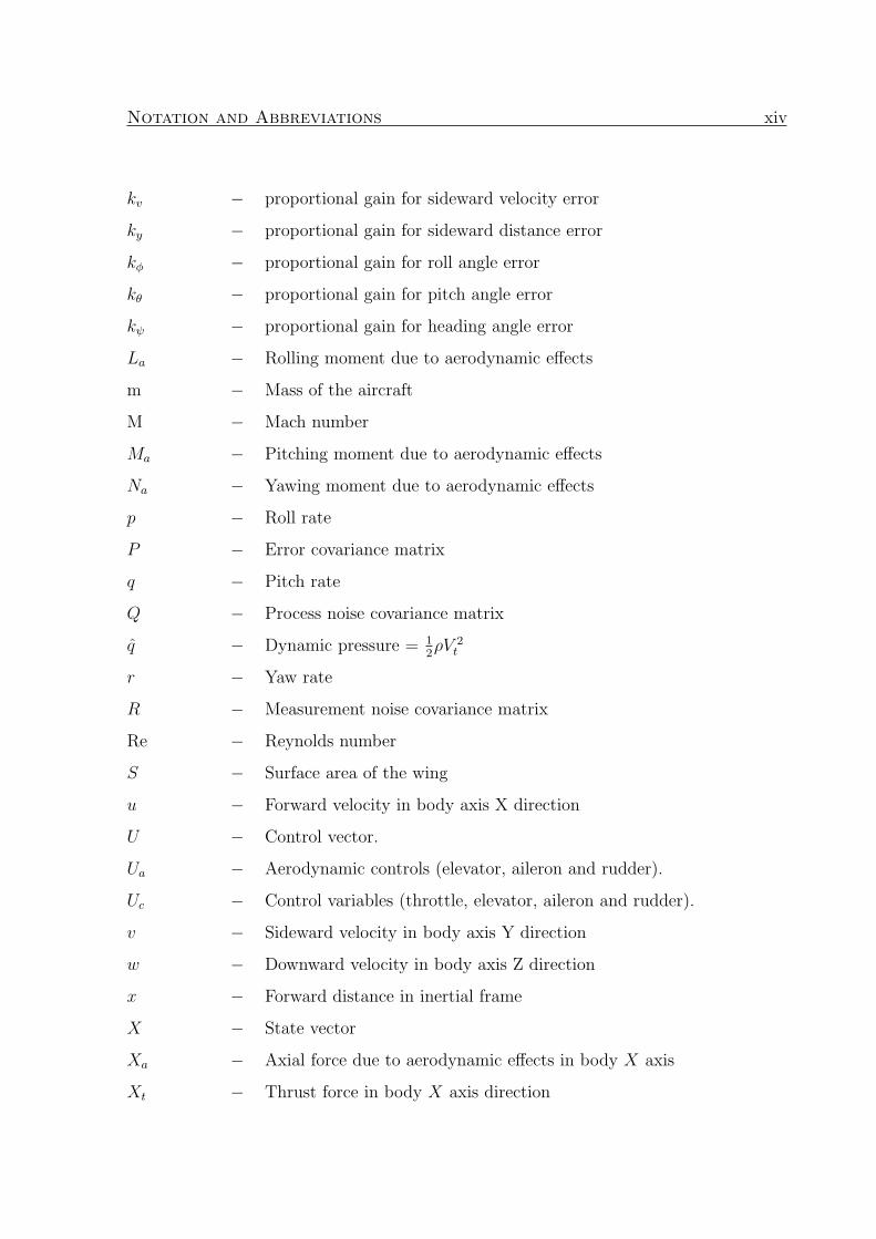
Chapter 2. Mathematical modeling 26
The dynamic derivatives are evaluated with respect to angle of attack. While considering
the dynamics effects it is assumed that only pitch rate effects the longitudinal coefficients
of normal force, axial force and pitching moment. Which can be written as
CZdyn= CZq q CXdyn
= CXq q Cmdyn= Cmq q
where as the coefficients effected by roll rate and yaw rate are side force, rolling moment
and yawing moment coefficient. For them the relation can be written as
CYdyn= CYp p + CYr r Cldyn
= CYp p + Clr r Cndyn= CYp p + Cnr r
The following sections give the results obtained for dynamic derivatives from AVL.
Pitch rate derivatives
The pitch rate derivatives are found at various angle of attack. Then a function is fit
which will be able to predict derivative for entire range of angle of attack. The results
are shown in Fig. 2.32 and the functions obtained from curve fit are given as
CZq , z40 + z41α CXq , x30 + x31α Cmq , m40 + m41α + m42α2
−5 0 5 10 15 204
6
8
α (deg)
CZ
q
AVLCurve fit
−5 0 5 10 15 20−5
0
5
α (deg)
CX
q
−5 0 5 10 15 20−14
−13.5
−13
α (deg)
Cm
q
Figure 2.32: Pitch rate derivatives

Chapter 2. Mathematical modeling 27
Roll rate derivatives
The results for roll rate derivatives are shown in Fig. 2.33 and the functions obtained
from curve fit are given as
CYp , y40 + y41α Clp , l30 + l31α + l32α2 Cnp , n30 + n31α + n32α
2
−5 0 5 10 15 20−0.5
0
0.5
α (deg)
CY
p
AVLCurve fit
−5 0 5 10 15 20−0.6
−0.5
−0.4
α (deg)
Clp
−5 0 5 10 15 20−0.5
0
0.5
α (deg)
Cnp
Figure 2.33: Roll rate derivatives
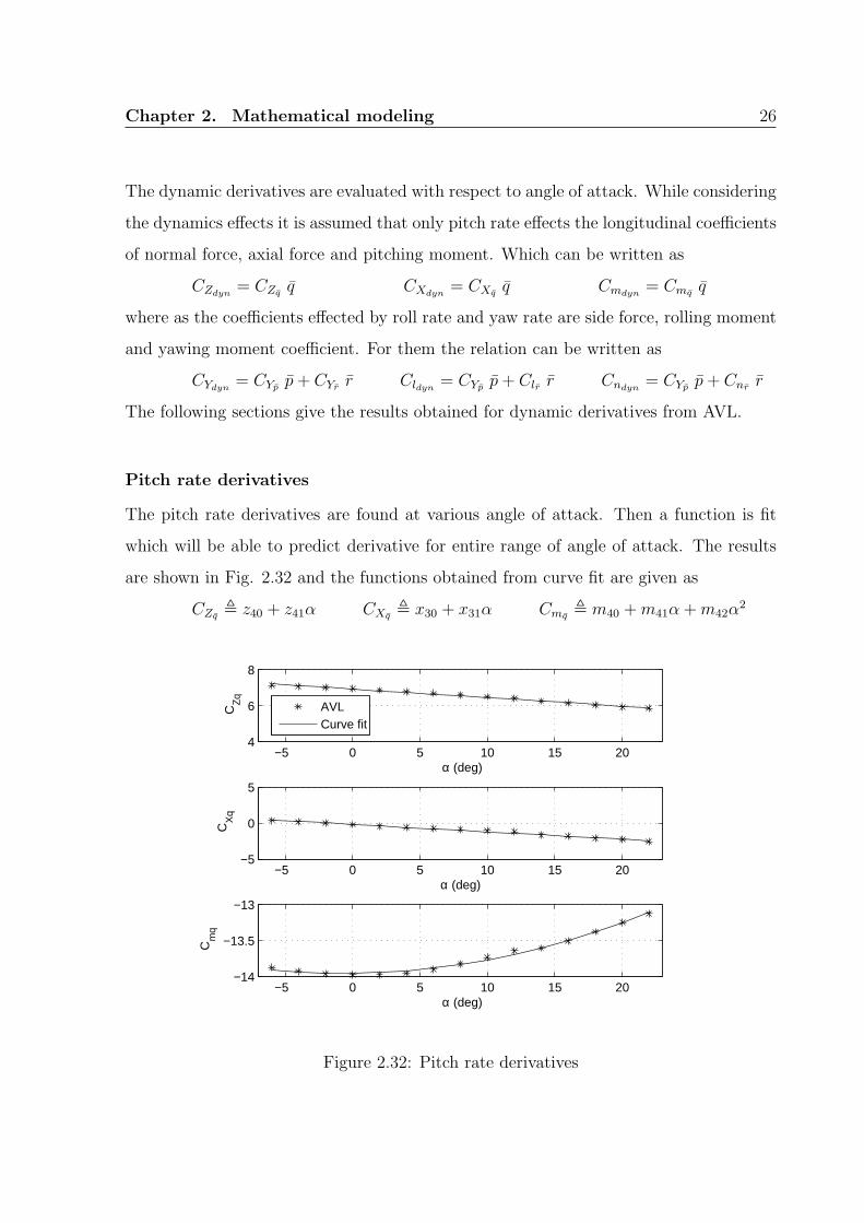
Yaw rate derivatives
The results for yaw rate derivatives are shown in Fig. 2.34 and the functions obtained
from curve fit are given as
CYr , y50 + y51α Clr , l40 + l41α + l42α2 Cnr , n40 + n41α + n42α
2
Chapter 2. Mathematical modeling 28
−5 0 5 10 15 200
0.2
0.4
α (deg)
CY
r
AVLCurve fit
−5 0 5 10 15 200
0.2
0.4
α (deg)
Clr
−5 0 5 10 15 20−0.4
−0.2
0
α (deg)
Cnr
Figure 2.34: Yaw rate derivatives
The aerodynamic coefficients with static and dynamic effects can be summarized as
CZ = CZ0 + CZα(α) α + CZββ + CZδe
δe + CZq(α) q (2.38)
CX = CX0 + CXα(α) α + CXδe(α) δe + CXq(α) q (2.39)
Cm = Cm0 + Cmα(α) α + Cmβ(α, β) β + Cmδe
(α) δe + Cmq(α) q (2.40)
CY = CYβ(α) β + CYδa
(α) δa + CYδr(α) δr + CYp(α)p + CYr(α) r (2.41)
Cl = Clβ(α) β + Clδa(α) δa + Clp(α) p + Clr(α) r (2.42)
Cn = Cnβ(α) β + Cnδr
(α) δr + Cnp(α) p + Cnr(α) r (2.43)
The Table 2.3 gives the value of average of absolute percentage error in the value obtained
by curve fitting and measured data.
Table 2.3: Average of absolute percentage error in curve fitting
α CZ CX Cm CY Cl Cn
−6o to 10o 6% 6% 16% 13% 11% 7%10o to 22o 23% 26% 27% 30% 25% 25%

Chapter 2. Mathematical modeling 29
The values of coefficients of the functions obtained by curve fit is given in Table 2.4.
Table 2.4: Derivatives function coefficient values
CZ0 0.1653 m12 -1.7853e-005 y24 -5.2196e-5 l30 -0.44336z10 0.087138 m13 -2.1109e-006 y25 8.8682e-6 l31 0.00075577z11 -0.0091867 m14 1.1346e-007 y26 -3.2717e-7 l32 -0.00013921z12 0.00024242 m20 0.00024049 y30 -0.0016884 l40 0.076582z20 -0.0020001 m21 -7.8566e-006 y31 -1.3637e-05 l41 0.010019z30 0.0039823 m22 1.0663e-006 y32 1.3214e-06 l42 1.1783e-005z40 6.9303 m23 -7.8866e-007 y40 -0.14504 n10 -0.0015474z41 -0.047657 m30 -0.0145 y41 0.013516 n11 6.1309e-005CX0 0.0386 m31 9.2552e-006 y50 0.13784 n12 -1.8989e-006x10 -0.0040376 m32 9.0437e-006 y51 0.0035514 n13 -5.5706e-006x11 -0.0010525 m40 -13.954 l10 0.0022856 n20 0.00077238x12 0.0027887 m41 0.0017379 l11 6.4827e-005 n21 1.1379e-006x13 0.00010917 m42 0.0016743 l12 -3.0529e-006 n22 -4.1705e-008x14 -5.3586e-6 y10 0.0099319 l13 -2.7687e-005 n30 -0.015512x20 -0.00035832 y11 0.00029462 l14 1.7713e-006 n31 -0.011325x21 -2.2061e-5 y12 1.7831e-005 l20 0.0029091 n32 9.8251e-005x22 -5.7342e-6 y13 -0.00030969 l21 9.0047e-006 n40 -0.085307x30 -0.18476 y14 1.6759e-005 l22 -7.4562e-006 n41 0.00080338x31 -0.10227 y20 0.0022145 l23 3.0423e-007 n42 -0.00026197Cm0 0.0346 y21 0.00041878 l24 -2.5531e-005m10 -0.013841 y22 1.3117e-5 l25 4.1263e-006m11 -0.00026206 y23 -1.1549e-6 l26 -2.0918e-007
2.3 Thrust force and moment
The AE-2 uses electric motor and propeller for thrust generation with lithium polymer
battery as its power source. The thrust force and moment are given as
Xt = (Tmax σt) (2.44)
Mt = −d (Tmax σt) (2.45)
where Tmax is the maximum thrust(15N) which can be produced by the electric motor
and propeller assembly. σt is throttle control which varies from 0 to 1. It is assumed
that thrust produced has linear relation with throttle input. d is offset (0.26m) of the
thrust line from the CG of the vehicle.

Chapter 2. Mathematical modeling 30
2.4 Actuator dynamics
The aerodynamic control surfaces are deflected by actuators. AE-2 employs electrome-
chanical servos for the control surface deflection, all the surfaces have the similar servo.
Here the actuator dynamics [30] for elevator servo is given
δe = bact δe + aact uδe (2.46)
where bact = −9.5, aact = 6.7 and uδe is the width of pulse width modulated (PWM)
signal. The step response of actuator is shown in the Fig. 2.35. The settling time for
the actuator is 0.54 seconds.
0 0.2 0.4 0.6 0.8 10
0.1
0.2
0.3
0.4
0.5
0.6
0.7
0.8
X: 0.54Y: 0.7011
time (sec)
Ser
vo d
efle
ctio
n (d
eg)
Figure 2.35: Step response of actuator
The thrust model can be implemented with first order lag. Where this lag is due
to time delay in increase or decrease of rotational speed of the propeller. This lag is
found from the manual of electric motor and speed controller through which the throttle
command is passed. The equation for thrust generation with first order lag can be
written as
T =1
τ(T − T ∗) (2.47)
where T is actual thrust, T ∗ is the commanded thrust and τ is the time constant.

Chapter 2. Mathematical modeling 31
2.5 Trim condition
The trim condition for steady and level flight can be found at a given velocity and
altitude. In order to find trim conditions we equate the dynamic equations to zero
(X = 0) and solve for the unknown variables. Here the given conditions are velocity
and altitude. The steady and level flight condition demand that the body angular rates
and roll angle be equal to zero (p = q = r = φ = 0). The unknown quantities to be
found are angle of attack, sideslip angle, pitch angle, throttle value and deflections of
elevator, aileron and rudder control. The equations used to solve for the unknowns are
[u v w p q r h] = 0, taken from the six-DOF equation of motion. Since the equations are
nonlinear the fsolve function of Matlab is used for finding solution. The trim conditions
at three different velocities and same altitude are found and given in table below.
Table 2.5: Trim conditions at different velocities
Vt h α β θ σt δe δa δr
m/s m deg deg deg (0-1) deg deg deg15 100 7.21 0 7.21 0.28 -9.81 0 020 100 3.15 0 3.15 0.36 -3.29 0 025 100 1.29 0 1.29 0.36 -1.17 0 0
The trim condition found can be verified with numerical simulation, by initializing the
system states with trim condition and integrating it for some time. The states of the
system will remain in the trim condition (Fig. 2.36 - 2.37) if the solution found is correct.
2.6 Simulation results
The open loop simulation and analysis is done in this section. There are twelve states
in the simulation and four controls
X = [u v w p q r φ θ ψ x y h] Uc = [σt δe δa δr]
The states u, v, w are replace by Vt, α, β in simulation results for better insight and
correlation. The results of the simulation have been clubbed in to three groups.
7→ Longitudinal states = (Vt α q θ x h) 7→ Lateral states = (β p r φ ψ y)
7→ Control variables = (σt δe δa δr)

Chapter 2. Mathematical modeling 32
2.6.1 Open loop simulation
The states are initialized with trim condition and simulated for 60 seconds. It is seen
from Fig. 2.36 and Fig. 2.37 that states continue to remain in trim condition.
0 20 4019
20
21
t (sec)
Vt (m
/s)
0 20 40 602
3
4
t (sec)
α (d
eg)
0 20 40 60−1
0
1
t (sec)
Q (d
eg/s
)
0 20 40 602
3
4
t (sec)
θ (d
eg)
0 20 40 600
500
1000
t (sec)
x (m
)
0 20 40 6099
100
101
t (sec)
h (m
)
Figure 2.36: Longitudinal states in trim condition
0 20 40 60−1
0
1
t (sec)
β (d
eg)
0 20 40 60−1
0
1
t (sec)
P (d
eg/s
)
0 20 40 60−1
0
1
t (sec)
R (d
eg/s
)
0 20 40 60−1
0
1
t (sec)
φ (de
g)
0 20 40 60−1
0
1
t (sec)
ψ (d
eg)
0 20 40 60−1
0
1
t (sec)
y (m
)
Figure 2.37: Lateral states in trim condition

Chapter 2. Mathematical modeling 33
2.6.2 Perturbation around trim condition
To study the stability of the system various perturbations are given around trim condi-
tion. A stable aircraft should return to the same or a near by equilibrium point after
oscillations. Fig. 2.38 and Fig. 2.39 show the stability of the vehicle with respect to
velocity, angle of attack, pitch angle and pitch rate perturbations.
0 50 10018
20
22
t (sec)
Vt (m
/s)
0 50 1002
4
6
t (sec) α
(deg
)
V
t(+2 m/s)
α(+2 deg)
0 50 100−10
0
10
t (sec)
Q (d
eg/s
)
0 50 100−20
0
20
t (sec)
θ (d
eg)
0 50 1000
2000
4000
t (sec)
x (m
)
0 50 10090
100
110
t (sec)
h (m
)
Figure 2.38: Effect of velocity and angle of attack perturbation on longitudinal states
0 50 10019
20
21
t (sec)
Vt (m
/s)
0 50 1002.5
3
3.5
t (sec)
α (d
eg)
θ(+3 deg)Q(−5 deg/s)
0 50 100−5
0
5
t (sec)
Q (d
eg/s
)
0 50 1000
5
10
t (sec)
θ (d
eg)
0 50 1000
2000
4000
t (sec)
x (m
)
0 50 10098
100
102
t (sec)
h (m
)
Figure 2.39: Effect of pitch angle and pitch rate perturbation on longitudinal states

Chapter 2. Mathematical modeling 34
Fig. 2.38 and Fig. 2.39 show the effect of sideslip and roll angle perturbation on the
states. It can be observed from the figures that the perturbation effects of sideslip are
highly damped compared to roll angle and they return to equilibrium very fast.
0 50 100−5
0
5
t (sec)
β (d
eg)
0 50 100−20
0
20
t (sec)
P (d
eg/s
)
β(+5 deg)
φ(+5 deg)
0 50 100−20
0
20
t (sec)
R (d
eg/s
)
0 50 100−5
0
5
t (sec)φ (
deg)
0 50 1000
100
200
t (sec)
ψ (d
eg)
0 50 100−2000
0
2000
t (sec)
y (m
)
Figure 2.40: Effect of sideslip and roll angle perturbation on lateral states
0 50 10019
20
21
t (sec)
Vt (m
/s)
0 50 1002
3
4
t (sec)
α (d
eg)
β(+5 deg)
φ(+5 deg)
0 50 100−2
0
2
t (sec)
Q (d
eg/s
)
0 50 1002
3
4
5
t (sec)
θ (d
eg)
0 50 1000
1000
2000
t (sec)
x (m
)
0 50 10099
100
101
t (sec)
h (m
)
Figure 2.41: Effect of sideslip and roll angle perturbation on longitudinal states
Summary: In this chapter the mathematical model for AE-2 has been developed. The
next chapter discusses the control design for inner and outer loop to track the guidance
commands along with velocity control.

Chapter 3
Control design
Various control strategies have been attempted to achieve the flight stabilization and
autonomous control for small unmanned aerial vehicles. Linear control theory has been
heavily investigated. Linear control theory has limitation of operation in linearization
range. To encompass the whole flight regime many such linear models would be required
with gain scheduling. Due to the limitations of linear control theory and the approxima-
tions involved in it, there has been a lot of research interest in nonlinear control design.
A popular method of nonlinear control design for tracking is the technique of dynamic
inversion. Which is based on the philosophy of feedback linearization. In this approach
an appropriate coordinate transformation is carried out followed by the application of
linear control theory. Here the feedback control cancels the nonlinearities in the plant
and closed loop plant behaves as a linear system. The limitation of this method is that
it requires an accurate knowledge of the plant model, in the absence of which the track-
ing will not be perfect. Dynamic inversion concept also involves the presence of hidden
zero dynamics. They must be examined separately to make certain that they are sta-
ble and well-behaved (analysis included at the end of this chapter). The mathematical
background for dynamic inversion [9], [10] is discussed in next Section.
3“The battlefield is a scene of constant chaos. The winner will be the one who controls that chaos,both his own and the enemies.” Napoleon Bonaparte(1769-1821)
35

Chapter 3. Control design 36
3.1 Dynamic inversion
Let us consider a nonlinear dynamical system which is affine in control and given by
following equations
X = f(X) + g(X)U (3.1)
Y = h(X) (3.2)
where X ∈ <n, U ∈ <m, Y ∈ <p are the state, control and output vectors of the nominal
system respectively. We assume the system is pointwise controllable. The objective is
to design a control U so that Y → Y ∗ as t →∞, where Y ∗ is the commanded signal for
the Y to track. We assume Y ∗ is bounded, smooth and slowly varying.
To achieve the above objective, it is noticed from Eq. 3.2, that using the chain rule
of derivative the expression for Y can be written as
Y = fY (X) + gY (X)U (3.3)
where fY , [ ∂h∂X
]f(X) and gY , [ ∂h∂X
]g(X). Next, defining E , (Y − Y ∗) the
controller is synthesized such that the following stable linear error dynamics is satisfied
E + KE = 0 (3.4)
The solution of the above differential equation is given as E = E0 exp−Kt. Where
K is chosen to be positive definite matrix. It can be chosen as diagonal matrix with
positive elements, where elements represent the ‘settling time constant’. Next, using the
definition of E and substituting the expression for Y from 3.3 in 3.4, we can obtain by
carrying out the algebra
gY (X)U = −fY (X)−K(Y − Y ∗) + Y ∗ (3.5)

Chapter 3. Control design 37
If p = m i.e. system has same number of controls as output and gY (X) is nonsingular
than we can obtain the control solution as
U = [gY (X)]−1[−fY (X)−K(Y − Y ∗) + Y ∗] (3.6)
The salient features of this method are that it provides a close form solution for the
controller and it can be implemented online without any computational difficulties. The
control solution also ensures that E → 0 as t → ∞, i.e. the asymptotic tracking
is achieved. However, the approach looks simple and it results in powerful nonlinear
controller, there are some important issues with this technique. First, is that it requires
p = m which may not hold good for all the dynamical systems. The second limitation
requires an accurate knowledge of the plant model, in the absence of which the tracking
will not be perfect. This deficiency can however be overcome by using the concepts of
robust control [31] or adaptive control [32].
The implementation of this method will require appearance of control term in dy-
namics after differentiation of output. The number of times output is differentiated to
get control term is known as ‘relative degree’. Sometimes this relative degree can be of
higher order. The other method to achieve this is through forming first order dynamics
in cascaded form using the concept of ‘time scale separation’. Here, the system is divided
into an inner and an outer loop (Fig. 3.1), where the dynamics in the inner loop has to
be faster than the dynamics in the outer loop.
Figure 3.1: Inner and outer loop structure

Chapter 3. Control design 38
A cascaded form of inner loop and outer loop also cancels the dynamics of a system,
but the cancellation is not exact. It relies on the approximation that the inner loop is so
fast, that the tracking in inner loop is achieved by the time new commands come from
outer loop. This can achieved by choosing the settling time constants of inner loop lower
than outer loop. The outer and inner loop control for the UAV is discussed in following
sections.
3.2 Outer loop control
The goal of outer loop control (Fig. 3.2) is to track the commands generated by guidance
loop. Where the guidance commands come from path planning which is discussed in next
Chapter. The commands from guidance are desired pitch angle (θ∗), desired roll angle
(φ∗) and desired heading angle (ψ∗). The outer loop achieves the tracking by converting
the guidance commands into desired body rates which are roll rate (p∗), pitch rate (q∗)
and yaw rate (r∗). These desired body rate signals are than fed to inner loop for tracking.
Figure 3.2: Outer loop control
The transformation of guidance commands to body rate commands is achieved by
enforcing first order error dynamics, which is discussed in following sections.

Chapter 3. Control design 39
3.2.1 Roll angle control
The roll angle can be controlled through roll rate command. The relative degree between
roll rate and roll angle is one. Hence to generate the roll rate command from error in
roll angle, we enforce the following first order error dynamics for roll angle error
(φ− φ∗) + kφ(φ− φ∗) = 0 (3.7)
where error = φ − φ∗ and φ∗ is the desired roll angle. kφ is chosen positive, given in
Table 3.1. Rearranging above equation we get
φ = φ∗ − kφ(φ− φ∗) (3.8)
From six-DOF equation of motion we have
φ = p + qsinφtanθ + rcosφtanθ (3.9)
Substituting φ equation in Eq. 3.8 and rearranging we get
p∗ = φ∗ − kφ(φ− φ∗)− (qsinφ + rcosφ)tanθ (3.10)
We have p∗ which is the required roll rate to achieve the desired roll angle.
3.2.2 Pitch angle control
The pitch angle can be controlled through pitch rate command. The relative degree
between pitch rate and pitch angle is one. Hence to generate the pitch rate command
from error in pitch angle, we enforce the following first order error dynamics for pitch
angle error
(θ − θ∗) + kθ(θ − θ∗) = 0 (3.11)
where error = θ − θ∗ and θ∗ is the desired pitch angle. kθ is chosen positive, given in
Table 3.1.

Chapter 3. Control design 40
Rearranging previous equation, we get
θ = θ∗ − kθ(θ − θ∗) (3.12)
From six-DOF equation of motion we have
θ = qcosφ− rsinφ (3.13)
Substituting θ equation in Eq. 3.12 and rearranging we get
q∗ = secφ(θ∗ −Kθ(θ − θ∗) + rsinφ) (3.14)
We have q∗ which is the required pitch rate to achieve the desired pitch angle.
3.2.3 Heading angle control
The heading angle can be controlled through yaw rate command. The relative degree
between yaw rate and heading angle is one. Hence to generate the yaw rate command
from error in heading angle, we enforce the first order error dynamics for heading angle
(ψ − ψ∗) + kψ(ψ − ψ∗) = 0 (3.15)
where error = ψ − ψ∗ and ψ∗ is the desired heading angle. kψ is chosen positive, given
in Table 3.1. Rearranging above equation we get
ψ = ψ∗ − kψ(ψ − ψ∗) (3.16)
From six-DOF equation of motion we have
ψ = qsinφsecθ + rcosφsecθ (3.17)
Substituting ψ equation in Eq. 3.16 and rearranging we get
r∗ = secφ cosθ(ψ∗ − kψ(ψ − ψ∗))− qtanφ (3.18)
We have r∗ which is the required yaw rate to achieve the desired heading angle.

Chapter 3. Control design 41
3.3 Inner loop control
The goal of inner loop (Fig. 3.3) is to track the body rate commands generated by outer
loop. The inner loop achieves the tracking by transforming the body rate commands
into aerodynamic controls. The body rate commands generated by outer loop control
are desired roll rate (p∗), desired pitch rate (q∗), and desired yaw rate (r∗). Where as
the aerodynamic controls are aileron (δa), elevator (δe) and rudder (δr) deflections.
Figure 3.3: Inner loop control
There is a separate loop for velocity control where velocity is maintained constant
through throttle control. The body rates control and velocity control are discussed in
following sections.
3.3.1 Body rates control
The aerodynamics controls should be calculated such that it tracks the body angular
rates desired by the outer loop. The relative degree between aerodynamic controls and
body rates is one. Hence enforce first order error dynamics for error in body rates
p− p∗
q − q∗
r − r∗
+
kp 0 0
0 kq 0
0 0 kr
p− p∗
q − q∗
r − r∗
= 0 (3.19)
where error = [(p− p∗) (q− q∗) (r− r∗)]T . kp, kq and kr are chosen positive (Table 3.1).

Chapter 3. Control design 42
Rearranging previous equation we get
p
q
r
=
p∗ − kp(p− p∗)
q∗ − kq(q − q∗)
r∗ − kr(r − r∗)
(3.20)
From six-DOF equation of motion we have
p = c1rq + c2pq + c3La + c4Na (3.21)
q = c5pr + c6(p2 − r2) + c7(Ma + Mt) (3.22)
r = c8pq − c2rq + c4La + c9Na (3.23)
Separating the state and control terms in p, q, r equations and rearranging Eq. 3.20 we
can writefr + grUa = br (3.24)
where Ua = [δa δe δr]T and other terms are defined as follows
fr ,
c1rq + c2pq + c3Lax + c4Nax
c5pr + c6(p2 − r2) + c7(Max −Mt)
c8pq − c2rq + c4Lax + c9Nax
gr ,
c3Lau 0 c4Nau
0 c7Mau 0
c4Lau 0 c9Nau
br ,
p∗ − kp(p− p∗)
q∗ − kq(q − q∗)
r∗ − kr(r − r∗)
Lax , qSb[Clβ(α) β + Clp(α) p + Clr(α) r] Lau , qSbClδa
Max , qSc[Cm0 + Cmα(α) α + Cmβ(α, β) β + Cmq(α) q] Mau , qScCmδe
Nax , qSb[Cnβ(α) β + Cnp(α) p + Cnr(α) r] Nau , qSbCnδr
Carrying out the necessary algebra in Eq. (3.24), the control solution is
Ua = g−1r (br − fr) (3.25)
The above solution for aerodynamic controls will track the desired body rates generated
by outer loop control.

Chapter 3. Control design 43
3.3.2 Forward velocity control
The forward velocity can be controlled by varying the thrust through throttle control.
The relative degree between throttle control and forward velocity is one. Enforcing the
following first order error dynamics for error in forward velocity
(u− u∗) + ku(u− u∗) = 0 (3.26)
where error = (u − u∗) and u∗ is the velocity which has to be maintained during the
flight. ku is chosen positive, given in Table 3.1. Rearranging above equation we get
u = u∗ − ku(u− u∗) (3.27)
From six-DOF equation of motion we have
u = rv − qw − gsinθ +Xa + Xt
m(3.28)
Substituting u equation in Eq. (3.27) and rearranging
fu + guσt = bu (3.29)
Where σt is throttle control value and other terms are defined as follows
fu , rv − qw − gsinθ +Xa
m
gu , Tmax
m
bu , u∗ − ku(u− u∗)
Rearranging the Eq. (3.29) we get the control solution as
σt = g−1u [bu − fu] (3.30)
The above solution for throttle control will track the desired velocity.

Chapter 3. Control design 44
3.4 Actuator controller
The control solutions found by inner loop are fed to actuator for deflection of aerodynamic
control surfaces. The actuator dynamics is given in Section 2.4 which is same for all
control surfaces. It is observed from the step response (Fig. 2.35) of actuator that it
has a settling time of 0.54 seconds. Which is higher than the desired settling time for
the inner loop, hence a first order controller is designed for the actuator. Enforcing first
order error dynamics for error in actuator deflection
(δe − δ∗e) + kδe(δe − δ∗e) = 0 (3.31)
where error = (δe − δ∗e) and δ∗e is the desired deflection for elevator. Substituting the
actuator dynamics given by Eq. 2.46 in above equation and rearranging we get
uδe =1
6.7[−9.5 δe + δ∗e − kδe(δe − δ∗e)] (3.32)
where uδe is the command to be fed to the actuator to achieve the desired deflection.
The response of actuator to 1 deg deflection command is shown in Fig. 3.4.
0 0.2 0.4 0.6 0.8 10
0.2
0.4
0.6
0.8
1
1.2
X: 0.22Y: 0.9931
time (sec)
Ser
vo d
efle
ctio
n (d
eg)
X: 0.54Y: 1
without controlwith control
Figure 3.4: Actuator response for 1 deg command of deflection

Chapter 3. Control design 45
3.5 Control structure
The Fig. 3.5 shows the combined inner and outer loop structure. Where roll angle, pitch
angle and heading angle command come from guidance. The commands from guidance
are converted into desired body rates by the outer loop. Further inner loop transforms
these desired body rates into required aerodynamic control surface deflections.
Figure 3.5: Control structure
The velocity control loop maintains the desired velocity by throttle control, not shown
in above figure. The various gains for control loops chosen after iterative simulation are
given in the table below.
Table 3.1: Gains for various control loops
kφ kθ kψ kp kq kr ku kδe
sec−1 sec−1 sec−1 sec−1 sec−1 sec−1 sec−1 sec−1
2 2 2 5 5 5 1 20
To test the control design done in above sections, simulations are carried out by
giving various commands. The simulations and resulting performance are presented in
next section.

Chapter 3. Control design 46
3.6 Simulation results
The simulation is initialized with the trim condition obtained in Section 2.5 as initial
conditions. After 5 seconds of simulation a sequence of 3-2-1-1 command is given where
the width of one unit has been kept as 5 seconds. The initial conditions are given below.
Initial states
X0 = [ Vt0 α0 β0 p0 q0 r0 φ0 θ0 ψ0 x0 y0 h0 ]
= [ 20 3.15o 0 0 0 0 0 3.15o 0 − 1200 0 100 ]
Initial control
Ua0 = [ σt0 δe0 δa0 δr0 ]
= [ 0.36 − 3.29o 0 0 ]
3.6.1 Pitch angle command
A 3-2-1-1 sequence for pitch angle command is given with ±5 deg around trim pitch
angle. The velocity control loop maintains the forward velocity as in trim condition.
The Fig. 3.6 shows the response of pitch angle to the command.
0 10 20 30 40 50−4
−2
0
2
4
6
8
10
t (sec)
θ (d
eg)
actualdesired
Figure 3.6: Pitch angle variation for 3-2-1-1 command

Chapter 3. Control design 47
It is seen from Fig 3.7 that the velocity is maintained constant and the altitude is
increasing at constant rate due to increase in pitch angle from the trim condition. The
Fig. 3.8 shows the control requirements. There is increased demand in negative elevator
for the positive pitching motion. The increase in elevator also increase drag hence more
of throttle is required to compensate for maintaining constant velocity.
0 10 20 30 4019
20
21
t (sec)
Vt (m
/s)
0 10 20 30 400
5
t (sec)
α (d
eg)
0 10 20 30 40
−10
0
10
t (sec)
Q (d
eg/s
)
0 10 20 30 40−2
02468
t (sec)
θ (d
eg)
0 10 20 30 40−1200−1000−800−600−400−200
t (sec)
x (m
)
0 10 20 30 40100
110
120
t (sec)
h (m
)
Figure 3.7: Longitudinal states for pitch angle command
0 10 20 30 400
0.2
0.4
0.6
0.8
1
t (sec)
σt (
0 −
1 )
0 10 20 30 40
−6
−4
−2
0
t (sec)
δe (d
eg)
0 10 20 30 40−1
−0.5
0
0.5
1
t (sec)
δa (d
eg)
0 10 20 30 40−1
−0.5
0
0.5
1
t (sec)
δr (d
eg)
Figure 3.8: Control variables for pitch angle command

Chapter 3. Control design 48
3.6.2 Heading angle command
A 3-2-1-1 sequence command for heading angle is given after 5 seconds of simulation
while the desire roll angle is zero and trim pitch angle is maintained. The Fig. 3.9 shows
the response of heading angle to ±5 deg command. It is seen from Fig. 3.10 that there
is small decrease in pitch angle this is due to reduction in lift during the turn.
0 10 20 30 40 50−6
−4
−2
0
2
4
6
t (sec)
ψ (d
eg)
actualdesired
Figure 3.9: Heading angle variation for 3-2-1-1 command
0 10 20 30 4019
20
21
t (sec)
Vt (m
/s)
0 10 20 30 402
3
4
t (sec)
α (d
eg)
0 10 20 30 40−1
0
1
t (sec)
Q (d
eg/s
)
0 10 20 30 402
3
4
t (sec)
θ (d
eg)
0 10 20 30 40−1200−1000−800−600−400−200
t (sec)
x (m
)
0 10 20 30 4099
100
101
t (sec)
h (m
)
Figure 3.10: Longitudinal states for heading angle command

Chapter 3. Control design 49
Fig. 3.11 shows the yaw rate required for the heading angle command. Also the
sideslip angle is non zero for some time as the coordinated turn constraint has not been
enforced. The control plots in Fig. 3.12 show the requirement in rudder deflection and
also aileron in an effort to maintain zero roll angle.
0 10 20 30 40
−5
0
5
t (sec)
β (d
eg)
0 10 20 30 40−2
0
2
t (sec)
P (d
eg/s
)
0 10 20 30 40
−10
0
10
t (sec)
R (d
eg/s
)
0 10 20 30 40−2
0
2
t (sec)
φ (d
eg)
0 10 20 30 40−5
0
5
t (sec)
ψ (d
eg)
0 10 20 30 400
10
20
t (sec)
y (m
)
Figure 3.11: Lateral states for heading angle command
0 10 20 30 400
0.2
0.4
0.6
0.8
1
t (sec)
σt (
0 −
1 )
0 10 20 30 40−5
−4
−3
−2
−1
t (sec)
δe (d
eg)
0 10 20 30 40
−5
0
5
t (sec)
δa (d
eg)
0 10 20 30 40
−10
−5
0
5
10
t (sec)
δr (d
eg)
Figure 3.12: Control variables for heading angle command

Chapter 3. Control design 50
3.6.3 Bank angle command
A 3-2-1-1 sequence command for roll angle is given while the desire heading angle is zero
and trim pitch angle is maintained. The response of roll angle to ±5 deg command is
shown in Fig. 3.13. It is seen from Fig. 3.14 though the pitch angle is constant, there is
constant decrease in altitude. It is due to reduction in lift due to non zero roll angle.
0 10 20 30 40 50−6
−4
−2
0
2
4
6
t (sec)
φ (d
eg)
actualdesired
Figure 3.13: Roll angle variation for step 3-2-1-1 command
0 10 20 30 4019
20
21
t (sec)
Vt (m
/s)
0 10 20 30 402
3
4
t (sec)
α (d
eg)
0 10 20 30 40−1
0
1
t (sec)
Q (d
eg/s
)
0 10 20 30 402
3
4
t (sec)
θ (d
eg)
0 10 20 30 40−1200−1000−800−600−400−200
t (sec)
x (m
)
0 10 20 30 4096
98
100
t (sec)
h (m
)
Figure 3.14: Longitudinal states for roll angle command

Chapter 3. Control design 51
Fig. 3.15 shows the roll angle is maintained without changing the heading angle.
However, this comes at a price of constant control effort for aileron and rudder deflections.
0 10 20 30 40
−5
0
5
t (sec)
β (d
eg)
0 10 20 30 40
−10
0
10
t (sec)
P (d
eg/s
)0 10 20 30 40
−1
0
1
t (sec)
R (d
eg/s
)
0 10 20 30 40−5
0
5
t (sec)
φ (d
eg)
0 10 20 30 40−1
0
1
t (sec)
ψ (d
eg)
0 10 20 30 400
10
20
30
t (sec)
y (m
)
Figure 3.15: Lateral states for roll angle command
0 10 20 30 400
0.2
0.4
0.6
0.8
1
t (sec)
σt (
0 −
1 )
0 10 20 30 40−4
−3
−2
−1
t (sec)
δe (d
eg)
0 10 20 30 40
−5
0
5
t (sec)
δa (d
eg)
0 10 20 30 40−15
−10
−5
0
5
10
t (sec)
δr (d
eg)
Figure 3.16: Control variables for roll angle command
Summary: The control has been designed in this chapter for inner and outer loop to
track the guidance commands along with velocity control. Next chapter discusses the
path planning and guidance command generation for autonomous landing.

Chapter 3. Control design 52
Appendix: Zero dynamics
The zero-dynamics is defined to be the internal dynamics of the system when the system
output is kept at zero by the input. The states of the system taken as output are
u, p, q, r, φ, θ, ψ, x, y, h. The remaining internal states are v and w. There dynamics is
given by following equations
v = pw − ru + gsinφcosθ +Ya
m(3.33)
w = qu− pv + gcosφcosθ +Za
m(3.34)
The input which keeps the outputs to zero can be calculated from Eq. 3.25 by putting
br = 0
Ua = g−1r (−fr) (3.35)
Now replacing the outputs as zero and the input given by above equation, we will get
v
w
=
[Avw
] v
w
Where Avw is linearized matrix around the initial condition and is given as
Avw =
∂f1
∂v∂f2
∂w
∂f1
∂v∂f2
∂w
The eigen values of the Avw matrix are tabulated for various operating points
Vt(m/s) h(m) λ1 λ2
15 100 -0.5397 -0.011120 100 -0.3148 -0.012525 100 -0.0128 -0.0011
It is observed from the above table that the eigen values of Avw matrix lie in left half
plane for the operating range of the UAV, hence the zero dynamics is locally stable.

Chapter 4
Path planning and guidance
The autonomous landing of UAVs require an intelligent path planning and guidance.
Here the landing is divided into three phases which are approach, glideslope and flare
(Fig. 4.1). The approach is initial phase of landing where UAV descents to a height from
which glideslope can begin while aligning itself with runway. The next is glideslope, a
straight line path where it looses most of its height. The last segment of landing is flare
which is an exponential curve at the end of which UAV touches down on ground. The
design and selection of the landing trajectory is discussed in next section.
Figure 4.1: Phases during landing
4“Our scientific power has outrun our spiritual power. We have guided missiles and misguided men.”Martin Luther King Jr.(1963)
53

Chapter 4. Path planning and guidance 54
4.1 Path planning
To guide the UAV it is required to specify the desired trajectory. The desired trajectory
can be made a function of time or distance in space. The trajectory tracking with respect
to time requires UAV to be in a particular location at particular point of time. There will
be problems in case of tracking a trajectory varying with time, when the UAV is flying
into wind disturbances [33]. To overcome this the effects of wind should be accounted
properly to move the desired trajectory slower or faster. To remove the dependence of
time a path in space can be specified, where UAV will be required to be on the path
rather than at a certain point on a particular time. Here the desired trajectory is made
a function of forward distance which is discussed in next sections.
4.1.1 Approach
During approach the vehicle should come and align with the runway at a specified height
from where the glideslope can be started. Fig. 4.2 shows the geometry for alignment
where (x0, y0) is the initial location of UAV at the beginning of landing. (xg, yg) is point
from where glideslope begins. ψ0 is the initial orientation of the vehicle.
y
runway x (0,0)
(x0,y
0)
(xg, y
g)
ψ0
Figure 4.2: Approach geometry in x-y plane (top view)

Chapter 4. Path planning and guidance 55
The initial condition (x0) for landing has bounds from which landing can be started
though there is no such constraint for the initial orientation (ψ0) and sideward distance
(y0). This constraint is due to the fact that UAV will require a minimum distance to take
turn and align before reaching the glideslope. The margin for initial condition has been
kept as (x0 − xg) > 400m, i.e. the alignment should begin 400m before the glideslope
initiation point. The equation for path of approach can be written as a straight line
function of forward distance.
y∗ = y0 +
(yg − y0
xg − x0
)(x− x0) (4.1)
This is the desired value of sideward distance during approach which UAV has to follow.
The desired value of sideward distance during glideslope and flare is zero (y∗ = 0) i.e.
aligned with the runway centerline. The UAV may also require to loose height during
approach to reach the glideslope height.
4.1.2 Glideslope
The glideslope is a straight line path whose slope is defined by the flight path angle. The
desired height is also scheduled as a function of forward distance.
(0, 0)
h(x
g, h
g)
(xf, h
f)
(x∞,h
c)
x γ∗
(xg0
, hg0
)
(xtd
, htd
)
Figure 4.3: Glideslope and flare geometry in x-h plane

Chapter 4. Path planning and guidance 56
In Fig. 4.3 (xg, hg) is the point where glideslope begins. (xf , hf ) is point where flare
begins. (xtd, htd = 0) is the touchdown point. (0, 0) is the origin of inertial frame at the
beginning of runway. (xg0 , hg0 = 0) is a fictitious point considered on ground from where
glideslope is projected. (x∞, hc) is the final point of flare path, this point is chosen to be
below ground so that exponential flare path intersects the ground at touchdown point.
From the geometry of the Fig. 4.3 the required flight path angle which vehicle has to
follow is calculated as follows
γ∗ = tan−1
(hg − hg0
xg − xg0
)(4.2)
The desired flight path angle (γ∗) which UAV has to follow is limited between 3o to 5o.
At lower flight path angle the position from which the glideslope has to begin (xg) will
become very large for a given glideslope altitude. At higher values of flight path angle
the vehicle will have limitation as the component of gravity will cause an increase in
velocity during landing. The desired height at every point of glideslope can be written
as a function of forward distance given by following equation
h∗ = hg0 + (x− xg0) tanγ∗ (4.3)
The UAV will follow the path specified by above equation while maintaining lateral error
to zero until the flare height is reached. The flare height is calculated online and it is
not fixed apriori which is discussed in next section.
4.1.3 Flare
The flare path is an exponential curve shown in Fig. 4.3. The exponential curve needs to
be chosen to end below the ground so that it touches the ground at a finite location. The
problem of slope discontinuity at the transition from glideslope to flare can be addressed
by appropriately choosing the parameters which specify the flare path. The advantage
of scheduling desired height as a function of forward distance is that we can specify the
location of touchdown. It is also required to control the sink rate at the touchdown in
order to avoid a hard landing.

Chapter 4. Path planning and guidance 57
The desired height during exponential flare can be scheduled as a function of forward
distance, given by following equation
h∗ = hc + (hf − hc)e−kx(x−xf ) (4.4)
The unknowns in above equation are flare height hf , distance at which to begin flare xf ,
final height below the ground where flare trajectory should end hc, and constant kx. We
can solve for these four unknowns under the following four constraints,
Initial condition: The point where glideslope ends and flare begins be coincident. Sub-
stituting x = xf in (4.3) and (4.4) than equating
hf = −(xf − xg0) tanγ∗ (4.5)
Initial slope: The slope at the beginning of flare and at the end of glideslope be same.
Differentiating (4.3) and (4.4) than equating at x = xf
(hf − hc)kx = tanγ∗ (4.6)
Touchdown condition: The flare trajectory should intersect the ground at touchdown
point. Replacing x = xtd and h∗ = 0 in (4.4) we get
0 = hc + (hf − hc)e−kx(xtd−xf ) (4.7)
Sink rate at touchdown: The descent rate at touchdown should be equal to specified sink
rate. Differentiating (4.4) and evaluating at x = xtd. Putting h∗ = h∗td, where h∗td is the
desired sink rate at touchdown. The ground velocity at touchdown (xtd) is taken as equal
to the air velocity controlled at touchdown.
h∗t = −(hf − hc)kxxtde−kx(xtd−xf ) (4.8)
Now we can solve the Eq. 4.5 - 4.8 for the four unknowns of the flare path. The solution
will ensure a smooth transition from glideslope to flare path. We also have the direct
control over the touchdown point and sink rate at touchdown. Which can be the design
parameters and tuned as per the requirement.

Chapter 4. Path planning and guidance 58
To closely follow the path specified by path planning, appropriate guidance commands
need to be generated which is discussed in next section.
4.2 Guidance
The desired values from path planning to be tracked are sideward distance (y∗ = 0) and
altitude (h∗ = 0). The kinematic equations for sideward distance and altitude can be
inverted to find the desired values of heading angle and pitch angle required for tracking.
While taking turn during approach the coordinated turn constraint is imposed from
which the desired roll angle can be found.
4.2.1 Sideward distance control
To track the desired sideward distance (y∗) we enforce a first order error differential
equation as
(y − y∗) + ky(y − y∗) = 0 (4.9)
where error = y − y∗. The gain ky is chosen positive, given in Table 4.1. Rearranging
above equation we get
y = y∗ − ky(y − y∗) (4.10)
From six-DOF equations we can write
y = ay sinψ + by cosψ (4.11)
where ay , u cosθ + v sinφsinθ + w cosφsinθ
by , v cosφ− w sinφ
Substituting Eq. (4.11) in Eq. (4.10) than solving for ψ
ψ∗ = sin−1
(y∗ − ky(y − y∗)√
a2y + b2
y
)− tan−1
(by
ay
)(4.12)
We have ψ∗ which is the required heading angle to track the path for sideward distance.

Chapter 4. Path planning and guidance 59
4.2.2 Altitude control
The altitude can be controlled by commanding pitch angle. The relative degree between
pitch angle and altitude is one. To generate the pitch angle command from error in
altitude, we enforce the first order error dynamics for altitude error
(h− h∗) + kh(h− h∗) = 0 (4.13)
where error = h−h∗ and h∗ is the desired altitude. The gain kh is chosen positive, given
in Table 4.1. Rearranging above equation we get
h = h∗ − kh(h− h∗) (4.14)
From six-DOF equations we can write
h = ahsinθ − bhcosθ (4.15)
where ah = u and bh = v sinφ + w cosφ
Substituting Eq. (4.15) in Eq. (4.14) than solving for θ
θ∗ = sin−1
(h∗ − kh(h− h∗)√
a2h + b2
h
)+ tan−1
(bh
ah
)(4.16)
Now θ∗ is the desired pitch angle required to track the desired altitude. The UAV should
touchdown on the ground at the end of flare with bounds on pitch angle. This is ensured
by passing the desired pitch angle through a limiter (20 5 θ∗ 5 80) when near to ground.
The other approach taken is to find the trim condition for a given pitch angle at the
touchdown. This trim condition will provide us with a desired velocity at the end of flare
which can be fed to velocity control loop for tracking.
It is seen from Eq. 4.12 and Eq. 4.16 that they involve inverse sine functions. The value
of quantities inside the inverse function need to be ensured less than equal to 1, else the
solutions will be imaginary. This can be achieved by careful selection of ky and kh.

Chapter 4. Path planning and guidance 60
4.2.3 Coordinated turn constraint
The coordinated turn requires the sideslip angle be equal to zero, equivalently it can
enforced by maintaining side velocity in body frame to be zero. This can be achieved
by finding an equivalent roll angle from the enforced first order error dynamics for side
velocity.
(v − v∗) + kv(v − v∗) = 0 (4.17)
where error = v − v∗ and v∗ = 0 is the desired side velocity. From six-DOF equations
of motion we have
v = pw − ru + gsinφcosθ +Ya
m(4.18)
Substituting Eq. 4.18 in Eq. 4.17 and than solving for φ, we will get
φ∗ = sin−1
(v∗ − kv(v − v∗) + ru− pw − Ya
m
gcosθ
)(4.19)
This desired roll angle will ensure the coordinated turn and sideslip angle to be zero.
Schematic of path planning and guidance
Fig. 4.4 shows the complete structure of path planning and guidance.
Figure 4.4: Path planning and guidance schematic

Chapter 4. Path planning and guidance 61
The gains used for path planning and guidance are given in the table below.
Table 4.1: Gains for guidance loop
ky kh kv
1 0.5 1
4.3 Simulation results
In this section the simulation results in a disturbance free environment are given for a
complete sequence of landing including approach, glideslope and flare. The ground roll
phase after the touchdown is not simulated. The results for three cases with different
initial conditions is given in Table 4.2. The plots 4.5 - 4.10 correspond to case I.
The simulation is initialized with trim condition and landing is commanded. The UAV
first aligns itself with runway than follows glideslope and flare as seen in Fig. 4.5.
−1500−1000
−5000
−100
−50
0
50
100
150
0
10
20
30
40
50
60
Down range (m) Cross range (m)
Alt
itu
de
(m)
Case 1Case 2
Figure 4.5: Landing trajectory in 3D

Chapter 4. Path planning and guidance 62
The Fig. 4.6 and Fig. 4.7 show the landing path in lateral and longitudinal plane.
−1500 −1000 −500 0−80
−60
−40
−20
0
20
40
60
80
100
120
x (m)
y (
m)
Case 1Case 2
Figure 4.6: Landing path in x-y plane
−1500 −1000 −500 0−10
0
10
20
30
40
50
60
70
x (m)
h (
m)
Case 1Case 2
Figure 4.7: Landing path in x-h plane
Fig. 4.8 shows the evolution of longitudinal states during landing. There are oscil-
lations observed in initial approach phase due to the coupling between longitudinal and
lateral dynamics, also the constant altitude is commanded during the turning maneuver.
0 20 40 60 8015
20
25
t (sec)
Vt (m
/s)
0 20 40 60 800
5
10
t (sec)
α (d
eg)
Case 1Case 2
0 20 40 60 80−20
0
20
t (sec)
Q (d
eg/s
)
0 20 40 60 80−10
0
10
t (sec)
θ (d
eg)
0 20 40 60 80−2000
0
2000
t (sec)
x (m
)
0 20 40 60 80−100
0
100
t (sec)
h (m
)
Figure 4.8: Longitudinal states during landing

Chapter 4. Path planning and guidance 63
Fig. 4.9 shows the evolution of lateral states during landing. The coordinated turn
constraint brings the sideslip angle during the turn close to zero.
0 20 40 60 80−5
0
5
t (sec)
β (d
eg)
0 20 40 60 80−100
0
100
t (sec)
P (d
eg/s
)
Case 1Case 2
0 20 40 60 80−20
0
20
t (sec)
R (d
eg/s
)
0 20 40 60 80−50
0
50
t (sec)φ
(deg
)
0 20 40 60 80−200
0
200
t (sec)
ψ (d
eg)
0 20 40 60 80−200
0
200
t (sec)
y (m
)
Figure 4.9: Lateral states during landing
Fig. 4.10 shows the control values during landing plotted with respect to forward dis-
tance. It is seen that there are oscillations in the initial approach phase while maintaining
constant altitude. The throttle requirement during glideslope has gone to idle position
(5%) as the commanded velocity is decreased (Fig. 4.8).
−1500 −1000 −500 00
0.2
0.4
0.6
0.8
1
x (m)
δt (
0 −
1 )
Case 1Case 2
−1500 −1000 −500 0
−20
−10
0
x (m)
δe (d
eg)
−1500 −1000 −500 0
−10
0
10
x (m)
δa (d
eg)
−1500 −1000 −500 0
−10
0
10
x (m)
δr (d
eg)
Figure 4.10: Control values during landing

Chapter 4. Path planning and guidance 64
The numerical results for the two cases of landing which have different initial conditions
is given in Table 4.2. The commanded values for path planning are given below.
(x∗g, y∗g , h
∗g) = (−1000, 0, 50) Location for end of approach and beginning of glideslope.
(x∗td, y∗td, h
∗td) = (50, 0, 0) Location for touchdown.
h∗td = −0.1 m/s Value of sink rate at touchdown.
The values achieved by UAV during simulation are given in table below. Where (xf , hf )
is location at which flare begins and θtd is the pitch angle at touchdown.
Table 4.2: Landing results
Initial Flare Touchdown
(x0, y0, h0) ψ0 (xf , hf ) xtd htd θtd
m deg m m m/s degCase 1 (-1500, 10, 50) 120o (-5.24, 14.04) 48.74 -0.10 5.55o
Case 2 (-1500, -50, 60) -45o (-4.88, 13.44) 49.06 -0.08 5.63o
It can be observed from the Table 4.2 that the commanded values of touchdown
location and sink rate at touchdown are closely followed. The pitch angle at touch down
was not enforced directly but it was solved for trim condition at touchdown with 6o of
pitch angle. The resulting solution for velocity was controlled at touchdown which has
resulted in pitch angles (θtd) close to 6o.
Summary: The path planning and guidance command generation for autonomous land-
ing has been discussed in this chapter and demonstrated through simulation. In next
chapter the state estimation has been done with Extended Kalman Filter, further the
design is tested in presence of wind disturbance.

Chapter 5
State estimation
The state feedback control laws require an estimate of the true state. There are many
uncertainties associated with the state estimation which make it a difficult problem. The
state estimation will depend upon the accuracy of mathematical modeling. The aero-
dynamic force and moment coefficients can not be modeled accurately even after wind
tunnel tests. There will also be process noise due to the presence of wind disturbances
which are not easy to measure. The sensors have measurement noise which will not give
the deterministic output. Kalman filter is an optimal estimator which minimizes the
variance of states error in the presence of process and measurement noise.
Kalman filter uses the knowledge of system and measurement dynamics, assumed
statistics of system disturbance and measurement errors with initial condition informa-
tion to arrive at optimal estimate. The Kalman filter was initially designed for linear
systems, further it has been modified for nonlinear systems called as Extended Kalman
Filter (EKF). The EKF minimizes the state estimation error with respect to the nonlin-
ear system’s linearized model. The mathematical background for EKF [23], [34] is given
in the next Section.
4“Position and velocity of a particle can not be measured accurately at the same time.” WernerHeisenberg(1927)
65

Chapter 5. State estimation 66
5.1 Extended Kalman Filter
In a dynamical system states are continuously evolving and the measurements arrive at
discrete intervals. Therefore continuous-discrete formulation of EKF best describes a
dynamical system. The nonlinear system model for estimation can be given by following
equations for states and outputs
X = f(X(t), Uc(t), t) + G(t)w(t) (5.1)
Yk = h(Xk) + vk (5.2)
Where, the vector f represents the system dynamics which is a nonlinear function of
the state X, the deterministic control input Uc and varies with time t. The disturbance
input or process noise w is white, zero mean gaussian random process. The statistical
properties of process noise can be written as,
E[w(t)] = 0 (5.3)
E[w(t)wT (t)] = Q (5.4)
The vector h represents the output equation which is a nonlinear function of the state
X. The measurement noise v is also white, zero mean gaussian random process that
is uncorrelated with disturbance input. The statistical properties of measurement noise
can be written as,
E[vk] = 0 (5.5)
E[vkvTk ] = R (5.6)
E[w(t)vTk ] = 0 (5.7)
The basic assumption in EKF is that the true state is sufficiently close to the estimated
state. Therefore, the error dynamics can be represented fairly accurately by a linearized
first-order Taylor series expansion. So we linearize the nonlinear system around the

Chapter 5. State estimation 67
Kalman filter estimate of the state. The linearized matrices also known as sensitivity
matrices are given as
F (t) =∂f
∂X|X(t)=X(t) (5.8)
H(t) =∂h
∂X|X(t)=X(t) (5.9)
The expected values of the initial state and its covariance are assumed known and given
by following equations
E(X0) = X0 (5.10)
E[(X0 − X0)(X0 − X0)T ] = P0 (5.11)
A weighting factor called the Kalman filter gain is computed using the covariance infor-
mation, output sensitivity matrix and the measurement covariance matrix . The Kalman
filter gain is used to combine the extrapolated estimate with the new measurement. This
gain is defined in such a way that it minimizes the estimation error covariance after the
update. The Kalman filter gain [23] is given by following equation
Kk = P−k HT
k (t−k ) [Hk(t−k ) P−
k HTk (t−k ) + Rk]
−1 (5.12)
New measurements are combined with the extrapolated estimate to generate an updated
estimated state. The state covariance also is updated to reflect the information contained
in the measurement. The state and covariance update equation are
X+k = X−
k + Kk [Yk − h(t−k )] (5.13)
P+k = [I −Kk Hk(t
−k )] P− (5.14)

Chapter 5. State estimation 68
The EKF propagates both the state estimate and its covariance using the system model
given by following equations
˙X(t) = f(X(t), Uc(t), t) (5.15)
P (t) = F (t) P (t) + P (t) F T (t) + G(t) Q(t) GT (t) (5.16)
The EKF algorithm involves initialization of states and covariance, computation of
Kalman filter gain, update of states and covariance followed by propagation of states and
covariance. This process is followed in a cyclic manner excluding initialization. Equa-
tions (5.9)-(5.16) constitute the EKF algorithm for continuous-time nonlinear systems
with discrete measurements.
5.2 Filter equations for UAV
The equations for UAV need to be modified in order to take in account the wind distur-
bance. This can be achieved by making the wind disturbances as a part of state vector,
which is discussed in following sections.
5.2.1 Wind disturbances
The wind disturbance is considered in inertial frame x, y and h directions. The natural
wind tends to be constant or slowly varying in horizontal plane where as there are wind
gusts in vertical direction. Therefore the wind in x and y direction are assumed to be
constant and wind in h direction accelerating. It is necessary to make these disturbances
part of the system state vector. The wind state vector is defined as
Xd = [wx wy wh wh] (5.17)
Any mathematical model of the wind dynamics represent an approximation to the con-
ditions that exist. Error in the modeling can lead to biases in the estimates and even

Chapter 5. State estimation 69
divergence from the actual values. Hence the dynamics of the wind [25] can be repre-
sented by using a simple Integral state model [36] given by following equations
Xd = FdXd + wd (5.18)
where
Fd =
0 0 0 0
0 0 0 0
0 0 0 1
0 0 0 0
wd =
0
0
0
1
To account the wind acceleration we transform it from inertial frame to body frame
aBw = [HB
I ]aIw
Where HBI is the transformation matrix from inertial frame to body frame and the
acceleration of wind disturbance is given as aIw , [ 0 0 wh ]. The transformation of
wind acceleration to body axis will give
aBwx
aBwy
aBwh
=
cosθcosψ cosθsinψ −sinθ
sinφsinθsinψ − cosφsinψ sinφsinθsinψ + cosφcosψ sinφcosθ
cosφsinθcosψ + sinφsinψ cosφsinθsinψ − sinφcosψ cosφcosθ
0
0
−wh
Simplifying above equation we will get
aBwx
= wh sinθ aBwy
= −wh sinφcosθ aBwh
= −wh cosφcosθ
5.2.2 State sensitivity matrix
To account for the wind and wind acceleration the translational dynamic and kinematic
equations are revised to wind relative reference frame [35].
Translational dynamics
ua = rva − qwa − gsinθ +Xa + Xt
m− aB
wx
va = pwa − rua + gsinφcosθ +Ya
m− aB
wy
wa = qua − pva + gcosφcosθ +Za
m− aB
wh

Chapter 5. State estimation 70
Translational kinematics
x = uacosθcosψ + va(sinφsinθsinψ − cosφsinψ) + wa(cosφsinθcosψ + sinφsinψ) + wx
y = uacosθsinψ + va(sinφsinθsinψ + cosφcosψ) + wa(cosφsinθsinψ − sinφcosψ) + wy
h = uasinθ − vasinφcosθ − wacosφcosθ + wh
The rotational dynamic and kinematic equations remain unchanged as given Chapter 2.
In above equations the ua, va, and wa are the wind relative body frame velocities. Now
the the system state vector is defined as
X = [ua va wa p q r φ θ ψ x y h] (5.19)
Combining the system and wind disturbance states, we can define
χ ,
X
Xd
(5.20)
The combined dynamics can be represented as
χ =
X
Xd
=
f(X,Uc, Xd)
FdXd
+
0
wd
(5.21)
The linearized matrix of state can be found as
F (t) =∂f
∂χ(5.22)
The expressions for linearized matrix is given in below equations
∂(ua, va, wa)∂χ =
0 r −q 0 −wa va 0 −(g − wh)cθ sθ
−r 0 p wa 0 −ua (g − wh)cθcφ −(g − wh)sθsφ 03×7 −sφcθ
q −p 0 −va ua 0 −(g − wh)cθsφ −(g − wh)sθcφ −cφcθ
3×16

Chapter 5. State estimation 71
∂(p, q, r)∂χ =
c2q c1r + c2p c1q
03×3 c5r − 2c6p 0 c5p + 2c6r 03×10
c8q c8p− c2r −c2q
3×16
∂(φ, θ, ψ)∂χ =
1 sφtθ cφtθ (qcφ − rsφ)tθ (qsφ + rcφ)se2θ
03×3 0 cφ −sφ −qsφ − rcφ 0 03×8
0 sφseθ cφseθ (qcφ − rsφ)seθ (qsφ + rcφ)seθtθ
3×16
∂(x, y, h)∂χ =
cθcψ sφsθcψ − cφsψ cφsθsψ − sφcψ
cθsψ sφsθsψ + cφcψ cφsθsψ − sφcψ 03×3 03×3 I3×3 03×1
sθ −sφcθ −cφcθ
3×16
∂(wx, wy , wh, wh)∂χ =
0
04×15 0
1
0
4×16
where, sφ , sinφ, sθ , sinθ, sψ , sinψ tθ , tanθ,
cφ , cosφ, cθ , cosθ, cψ , cosψ seθ , secθ
The state sensitivity will be given as
F (t) = ∂f∂χ
=
∂(ua, va, wa)∂X
∂(p, q, r)∂X
∂(φ, θ, ψ)∂X
∂(x, y, h)∂X
∂(wx, wy, wh, wh)
∂X
16×16
5.2.3 Output sensitivity matrix
The sensors available for measurement are accelerometers, rate gyros, GPS, magnetome-
ter and pressure sensors which provide air velocity and altitude.

Chapter 5. State estimation 72
The output vector can be written as
Y = [vt ax ay az p q r ψ x y h] (5.23)
The output sensitivity matrix can be found as
H(t) =∂h
∂χ(5.24)
The expressions for linearized matrix is given in below equations
∂(vt, ax, ay az)∂χ =
ua
vt
ua
Vt
ua
Vt0 0 0 0 0 0
0 −r q 0 wa −va 0 (g − wh)cθ −sθ
r 0 −p −wa 0 ua −(g − wh)cθcφ (g − wh)sθsφ 04×7 sφcθ
−q p 0 va −ua 0 (g − wh)cθsφ (g − wh)sθcφ cφcθ
4×16
∂(p, q, r)∂χ =
03×3 I3×3 03×10
3×16
∂(ψ, x, y, h)∂χ =
04×8 I4×4 04×4
4×16
The output sensitivity will be given as
H(t) = ∂h∂X
=
∂(vt, ax, ay az)
∂χ
∂(p, q, r)∂X
∂(ψ, x, y, h)∂X
11×16

Chapter 5. State estimation 73
5.2.4 Selection of R, P0 and Q
The outputs given by the onboard sensors are accelerations, body rates, air velocity,
altitude and ground position given by GPS. The sensors give output at a frequency of
50hz other than GPS whose data arrive at 5hz. Hence the algorithm uses the inertial data
until the GPS measurements arrive, than the positions are corrected. The measurement
noise covariance matrix obtained from the given specifications of the sensors is
R = diag(22, 12, 12, 12, 0.022, 0.022, 0.022, 0.052, 52, 52, 52) (5.25)
The initial error covariance was selected by trial and error and finally set to P0 = I. If the
initial covariance was made large, than states showed large oscillations in transient and
filter diverged in some cases. The smaller values of covariance delayed the convergence
of estimated states to the actual states.
The process noise covariance is set to
Q = diag(0, 0, 0, 0, 0, 0, 0, 0, 0, 0, 0, 0, 0.1, 0.1, 0, 0.001) (5.26)
The zero elements in the diagonal terms represent there is no process noise in that channel
of state. The nonzero diagonal elements were determined through trial-and-error. If they
were made too large, the EKF attenuated the measurement noise and very small diagonal
elements introduced significant lags into the estimates of the states.
5.3 Simulation results
The simulation results are shown here in presence of wind disturbance. The plots show
the comparison of performance between ideal conditions when there is no wind and the
states are known perfectly and the actual conditions when the state is estimated in
presence of wind disturbances and measurement noise. The landing command is given
after 5 seconds of simulation. This lead time is required for the settling of filter gains.

Chapter 5. State estimation 74
Fig. 5.1 shows the comparison of landing path when there is no wind and states are
known perfectly and when there are wind disturbances and state is estimated.
−1500−1000
−5000
0
50
100
0
10
20
30
40
50
Forward distance (m) Sideward distance (m)
Alti
tude
(m
)
IdealActual
Figure 5.1: Landing trajectory in 3D with EKF
The Fig. 5.2 and Fig. 5.3 show the landing path in lateral and longitudinal plane. In
Fig. 5.3 it is seen that altitude drops initially as the wind is introduced, this leads to
decrease in air relative velocity hence the lift generated decreases.
−1600 −1400 −1200 −1000 −800 −600 −400 −200 0
0
20
40
60
80
100
120
X (m)
Y (
m)
IdealActual
Figure 5.2: Landing path in x-y plane
−1600 −1400 −1200 −1000 −800 −600 −400 −200 00
5
10
15
20
25
30
35
40
45
50
X (m)
h (
m)
IdealActual
Figure 5.3: Landing path in x-h plane

Chapter 5. State estimation 75
The Fig. 5.4 shows the estimation error in longitudinal states. It is seen that all the
states remain in the bound other than pitch rate, which is due to the wind acceleration
in pitch plane.
0 20 40 60−2
0
2
t (sec)
U (m
/s)
0 20 40 60−2
0
2
t (sec)
W (m
/s)
0 20 40 60−5
0
5
t (sec)
θ (d
eg)
0 20 40 60−5
0
5
t (sec) Q
(deg
/s)
error
3 σ
0 20 40 60−5
0
5
t (sec)
x (m
)
0 20 40 60−5
0
5
t (sec)
h (m
)
Figure 5.4: Estimation error in longitudinal states
The Fig. 5.5 shows the estimation error in lateral states. It is seen that all the states
remain in the bound other than heading angle which takes some time.
0 20 40 60−2
0
2
t (sec)
β (de
g)
0 20 40 60−10
0
10
t (sec)
P (d
eg/s
)
error3 σ
0 20 40 60−10
0
10
t (sec)
R (d
eg/s
)
0 20 40 60−10
0
10
t (sec)
φ (de
g)
0 20 40 60−1
0
1
t (sec)
ψ (d
eg)
0 20 40 60−5
0
5
t (sec)
y (m
)
Figure 5.5: Estimation error in lateral states

Chapter 5. State estimation 76
The Fig. 5.6 shows the estimation of wind disturbances. It can be observed that the
estimated states follow the actual wind with minimum error.
0 20 40 60−5
0
5
10
t (sec)
Wx (m
/s)
error3 σ
0 20 40 60−4
−2
0
2
4
t (sec)
Wy (m
/s)
0 20 40 60−4
−2
0
2
4
t (sec)
Wh (m
/s)
0 20 40 60−4
−2
0
2
4
t (sec)
Whd
ot (m
/s2 )
Figure 5.6: Wind estimation with EKF
The control values required with and without the disturbance are shown in Fig.5.7.
It is seen that there is continuous demand in control even during glideslope and flare
this is due to changing wind and wind gust.
0 20 40 600
0.5
1
t (sec)
δt (
0 −
1 )
IdealActual
0 20 40 60−30
−20
−10
0
10
t (sec)
δe
(deg
)
0 20 40 60−10
−5
0
5
10
t (sec)
δa
(deg
)
0 20 40 60−10
−5
0
5
10
t (sec)
δr (
deg)
Figure 5.7: Control values during landing with EKF

Chapter 5. State estimation 77
To test the algorithm a large number (100) of simulations were carried out. The
Fig. 5.8 shows the touchdown locations for various cases. To measure the performance
a successful landing zone is defined as shown in Fig. 5.8.
0 10 20 30 40 50 60 70 80−5
−4
−3
−2
−1
0
1
2
3
4
5
X (m)
Y (m
)
50m
6m
Successful landing zone
Figure 5.8: Touchdown position in x-y plane
The sink rate at touchdown and pitch angle bounds are specified for successful land-
ing. The large sink rate can cause damage to structure and lower sink rate can be carried
away by wind gust. At negative pitch angle the nose will touch first and at higher angle
the tail boom will touch the ground before wheels.
0 20 40 60 80 1000
1
2
3
4
5
6
7
8
9
10
no. of simulations
pitch
an
gle
at
tou
ch
do
wn
(d
eg
)
Figure 5.9: Pitch angle at touch down
0 20 40 60 80 100
−1
−0.8
−0.6
−0.4
−0.2
0
no. of simulations
sin
k r
ate
at to
uch
do
wn
(m
/s)
Figure 5.10: Sink rate at touch down

Chapter 5. State estimation 78
Parameter uncertainty
The uncertainty in the aerodynamic model is one of the key difficulties in the imple-
mentation of the dynamic inversion and extended kalman filter. The uncertainty in
parameters can be accommodated by considering fictitious process noise wf in the sys-
tem model [25]. The uncertainty in the system model is considered as gaussian random
input. The system dynamic equations which use the aerodynamic coefficients are added
with fictitious random noise. The revised model can be expressed as
χ =
X
Xd
=
f(X, Uc, Xd)
FdXd
+
wf
wd
(5.27)
The elements of process noise covariance matrix (Q) will have to be revised and chosen to
reflect the uncertainty in aerodynamic coefficients. The process noise covariance matrix
was chosen by trial and error while increasing the uncertainty in the coefficients. The
maximum percentage uncertainty accommodated by EKF was found to be 4%. Further
this was found to increase up to 6% with inclusion of integrator in the inner most loop.
The corresponding process noise covariance matrix is found as
Q = diag(0.001, 0.001, 0.2, 0.02, 0.05, 0.02, 0, 0, 0, 0, 0, 0, 0.1, 0.1, 0, 0.001)
The Fig. 5.11 shows the touchdown location for hundred simulations cases with the
uncertainty in parameters. It can be observed that the dispersion of landing location
has increased compared to when the uncertainty was not considered.
−10 0 10 20 30 40 50 60 70 80−6
−4
−2
0
2
4
6
X (m)
Y (m
)
Successful landing zone
Figure 5.11: Touchdown position in x-y plane with parameter uncertainty

Chapter 5. State estimation 79
The Fig. 5.12 and Fig. 5.13 show the pitch angle and sink rate at touchdown when
the uncertainty in the parameters is considered.
0 20 40 60 80 1000
1
2
3
4
5
6
7
8
9
10
no. of simulations
pitch
an
gle
at
tou
ch
do
wn
(d
eg
)
Figure 5.12: Pitch angle at touch down
0 20 40 60 80 100−1.4
−1.2
−1
−0.8
−0.6
−0.4
−0.2
0
no. of simulations
sin
k r
ate
at to
uch
do
wn
(m
/s)
Figure 5.13: Sink rate at touch down
The results obtained from simulations with the percentage of successful landing cases
is given in Table 5.1. The success criteria is defined as below
7→ For touch down location, 20m 5 xtd 5 70m and −3m 5 ytd 5 3m
7→ For pitch angle, 2odeg 5 θtd 5 8o
7→ For sink rate, −0.1m/s 5 htd 5 −1m/s
Table 5.1: Percentage of successful landing
touchdown pitch angle sink rate overallEKF with only disturbance 76% 79% 85% 71%
EKF with disturbance and uncertainty 69% 63% 64% 60%
It can be observed from the table that with parameter uncertainty in the aerodynamic
coefficients the percentage of successful landing has decreased. The success criteria can
be further relaxed with respect to sink rate and touchdown location.
Summary: In this chapter the state estimation has been done with Extended Kalman
Filter. Further the design is tested in presence of wind disturbances and parameter
uncertainty. The next chapter gives the conclusion of the research work done.

Chapter 6
Conclusions
In this thesis the problem of autonomous landing of unmanned aerial vehicles has been
addressed. The complete work has involved Mathematical modeling, Control design,
Guidance and State estimation. The guidance and control technique developed has been
demonstrated through numerical simulations using the data of an UAV named AE-2.
The curve fitting is done on the wind tunnel data of AE-2 obtained by static tests.
The method of least squares is used for minimizing the error in prediction and the
nonlinearities in the function obtained are reported. Further the dynamic derivatives are
found through AVL software which has been validated by comparison of static coefficients
obtained by the wind tunnel tests and vortex lattice method. The dynamics of thrust
and servo actuators have been incorporated in the simulation.
The control has been designed using nonlinear dynamic inversion technique. The
control is structured in outer loop and inner loop. The goal of outer loop is to track
the guidance commands by converting them into body rates. The inner loop tracks the
body rate commands by finding the required deflection of control surfaces. The forward
velocity of the vehicle is controlled by throttle. A controller for actuator is also designed
to reduce the lag.
80

Chapter 6. Conclusions 81
The guidance for landing is divided into three phases which are approach, glideslope
and flare. The desired trajectory for the landing has been made independent of time by
scheduling the trajectory as a function of forward distance from runway. The problem
of transition between the glideslope and flare has been addressed by ensuring continuity
and smoothness at transition. The location of touchdown on runway and the sink rate
at touchdown are controlled.
The state estimation has been done with EKF in continuous discrete formulation.
The external disturbances like wind shear and wind gust are accounted by appending
them in state variables. Further the control design with guidance is tested from various
initial conditions, in presence of wind disturbances. The designed filter has also been
tested for parameter uncertainty.

References
[1] A. Pelletier and T J. Mueller, Low Reynolds Number Aerodynamics of Low-Aspect-
Ratio Thin/Flat/Cambered-Plate Wings, Journal of Aircraft, vol.37, no.5, pp. 825-
832, 2000.
[2] E. A. Morelli, Global Nonlinear Parametric Modeling With Application to F-16
Aerodynamics, Proceedings of the American Control Conference, vol. 2, pp. 997-1001,
1998.
[3] G. C. Rufolo, P. Roncioni, M. Marini, R.Votta and S. Palazzo, Experimental and
Numerical Aerodynamic Data Integration and Aerodatabase Development for the
PRORA-USV-FTB1 Reusable Vehicle, 14th AIAA/AHI Space Planes and Hypersonic
Systems and Technologies Conference, 2006.
[4] R. Albertani, R. DeLoach, B. Stanford, J. P. Hubner and P. Ifju, Wind Tunnel
Data Base Development and Nonlinear Modeling Applied to Powered Micro Air Ve-
hicles with Flexible Wing, AIAA Atmospheric Flight Mechanics Conference and Exhibit,
Keystone, Colorado, 2006.
[5] J. S. Shamma and M. Athans, Analysis of Gain Scheduled Control for Nonlinear
Plants, IEEE Transactions On Automatic Control, vol. 35, no. 8, pp. 898-907, 1990.
[6] P. Rosa, C. Silvestre, D. Cabenchias and R. Cunha, Autolanding Controller for a
Fixed Wing Unmanned Air Vehicle, AIAA Guidance Navigation and Control Confer-
ence and Exhibit, 2007, Hilton head, South Carolina.
82

REFERENCES 83
[7] R. Wang and Y. Shen, Flying-Wing UAV Landing Control and Simulation Based
on Mixed H2/H∞, Proceedings of IEEE International Conference on Mechatronics and
Automation, Harbin, China, 2007.
[8] S. P. Shue, R. K. Agarwalt and Y. H. Kuo, Design of Automatic Landing Systems
using Mixed H2/H∞ Control, Aerospace Sciences Meeting and Exhibit, 36th, Reno,
Nevada, 1998
[9] D. Enns, D. Bugajski, R. Hendrick and G. Stein, Dynamic Inversion: An Evolving
Methodology for Flight Control Design, International Journal of Control, vol.59, no.1,
pp.71-91, 1994.
[10] J. J. E. Slotine and W. Li, Applied Nonlinear Control, Prentice Hall, 1991.
[11] B. Prasad and S. Pradeep, Automatic Landing System Design using Feedback Lin-
earization Method, Proceedings of AIAA Infotech Aerospace Conference and Exhibit,
Rohnert Park, California, 2007.
[12] C. Ha and H. Choi, Design of longitudinal autolanding guidance and control system
in dynamic model inversion, Proceedings of 6th Russian-Korean International Sympo-
sium on Science and Technology, pp. 7-10, 2002.
[13] M. J. Smith, S. S. M. Swei and M. B. Tischler, A Study of the Control of Micro Air
Vehicles Using the Linear Dynamic Inverse Approach, AIAA 1st Intelligent Systems
Technical Conference, Chicago, Illinois, 2004.
[14] M. Sadraey and R. Colgren, Robust Nonlinear Controller Design for a Complete
UAV Mission, AIAA Guidance, Navigation, and Control Conference and Exhibit, Key-
stone, Colorado, 2006.
[15] F. Lavergne, F. Villaume, M. Jeanneau, S. Tarbouriech and G. Garcia, Nonlinear
Robust Autoland, AIAA Guidance, Navigation, and Control Conference and Exhibit,
San Francisco, California, 2005.

REFERENCES 84
[16] K. S. Kumar and J.Shanmugam, Design of Blending function for landing phase of
an Unmanned Air Vehicle, Proceedings of AIAA Infotech Aerospace Conference and
Exhibit, Rohnert Park, California, 2007.
[17] J. G. Juang, H. H. Chang and K. C. Cheng, Intelligent Landing Control Using
Linearized Inverse Aircraft Model, Proceedings of the American Control Conference,
pp. 3269-3274, 2002.
[18] J.F. Vasconcelos, C. Silvestre, P. Oliveira, Embedded Vehicle Dynamics and LASER
Aiding Techniques for Inertial Navigation Systems, AIAA Guidance, Navigation, and
Control Conference and Exhibit, Keystone, Colorado, 2006.
[19] O. Shakernia, Yi Ma, T. J. Koo and S. Sastry, Landing an Unmanned Air Vehicle:
Vision Based Motion Estimation and Nonlinear Control, Asian Journal of Control,
Vol. 1, pg. 128-145, 1999.
[20] S. Saripalli, J. F. Montgomery and G. S. Sukhatme, Visually-Guided Landing of an
Unmanned Aerial Vehicle, Asian Journal of Control, IEEE Transactions on Robotics
and Automation, Vol. 19, No. 3, pg. 371-381, June 2003.
[21] T. G. Amaral, V. F. Pires and M. M. Crisostomo, Autonomous Landing of an Un-
manned Aerial Vehicle, Asian Journal of Control, Proceedings of the 2005 IEEE Interna-
tional Conference on Computational Intelligence for Modelling, Control and Automation,
2005.
[22] D. Blake Barber, S. R. Griffiths, T. W. McLain and R. W. Beard, Autonomous
Landing of Miniature Aerial Vehicles, AIAA Journal of Aerospace Computing, Infor-
mation, and Communication, Vol. 4, pg. 770-784, 5 May 2007.
[23] J. L. Crassidis and J. L. Junkins, Optimal Estimation of Dynamical Systems , CRC
Press LLC, 2004.
[24] S. S. Mulgund and R. F. Stengel, Aircraft Flight Control in Wind Shear Using

REFERENCES 85
Sequential Dynamic Inversion, Journal of Guidance, Control, and Dynamics, vol. 18,
no. 5, pp.1084-91, 1995.
[25] S. S. Mulgund and R. F. Stengel, Optimal Nonlinear Estimation for Aircraft Flight
Control in Wind Shear, Automatica, vol. 32, no. 1, pp. 3-13, 1996.
[26] C. Grillo and F. P. Vitrano, State Estimation of a Nonlinear Unmanned Aerial
Vehicle Model using an Extended Kalman Filter, AIAA International Space Planes
and Hypersonic Systems and Technologies Conference, Dayton, Ohio, 2008.
[27] V. Surendra nath, S. P. Govindaraju, M. S. Bhat, C. S. N. Rao, Configuration
Development of All Electric Mini Airplane, ADE/DRDO Project, 2004, Project Ref.
No: ADEO/MAE/VSU/001, Department of Aerospace Engineering, Indian Institute
of Science, Bangalore.
[28] B. L. Stevens and F. L. Lewis, Aircraft Control and Simulation, John Wiley and
sons Inc, 2nd edition, 2003.
[29] M. Drella and H. Youngren, Athena Vortex Lattice Analysis 3.26 User Primer,
http://web.mit.edu/drela/Public/web/avl/, April 2006
[30] M. Meenakshi and M. S. Bhat, Robust fixed-order H2 controller for micro air vehicle-
design and validation, Optimal Control Applications and Methods, vol. 27, pp. 183-210,
2006.
[31] G. J. Balas, W. L. Garrard and J. Reiner, Robust Dynamic Inversion Control Laws
for Aircraft Control, AIAA Guidance, Navigation and Control Conference, Hilton Head
Island, SC, Aug 10-12, 1992.
[32] R. Padhi and M. Kothari, An Optimal Dynamic Inversion Based Neuro-Adaptive
Approach for Treatment of Chronic Myelogenous Leukemia, Computer Methods and
Programs in Biomedicine, vol.87, pp. 208-228, 2007.

REFERENCES 86
[33] D. R. Nelson, D. B. Barber, T. W. McLain and R. W. Beard, Vector Field Path
Following for Miniature Air Vehicles, IEEE Transactions on Robotics, vol. 23, no. 3,
2007.
[34] R. F. Stengel, Optimal Control and Estimation, Dover publications, 1994.
[35] R. F. Stengel, Flight Dynamics, Princeton University Press, 2004.
[36] J. Bossi and A. E. Bryson, Disturbance estimation for a STOL transport during
landing, 19th Aerospace Sciences Meeting, St Louis, MO, 1981.


![Curve Tracing[MS Thesis]](https://static.fdocuments.net/doc/165x107/577d21db1a28ab4e1e960912/curve-tracingms-thesis.jpg)