MR99-K02 Preliminary Cruise Report - GODAC Data … Preliminary Cruise Report Contents 1. Preface 1...
168
MR99-K02 Preliminary Cruise Report June 1999 Japan Marine Science and Technology Center
Transcript of MR99-K02 Preliminary Cruise Report - GODAC Data … Preliminary Cruise Report Contents 1. Preface 1...
MR99-K02
Preliminary Cruise Report
June 1999
Japan Marine Science and Technology Center
MR99-K02 Preliminary Cruise Report
Contents
1. Preface -------------------------------------------------------------------------------------------------------- 1
2. Outline of MR99-K02
2.1 Cruise summary --------------------------------------------------------------------------------- 2
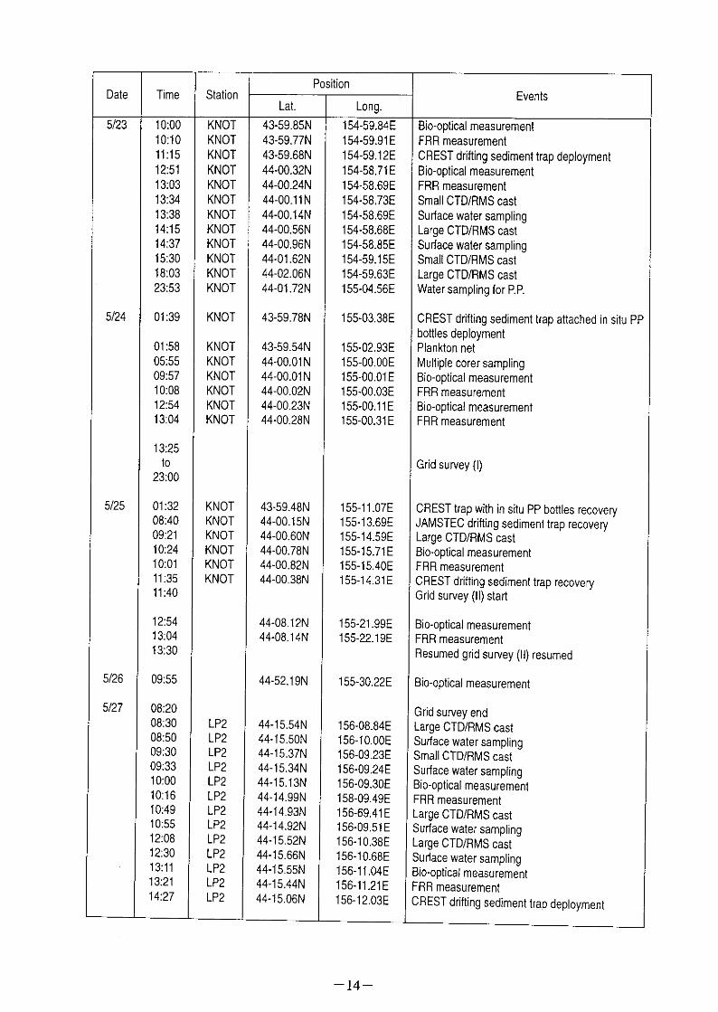
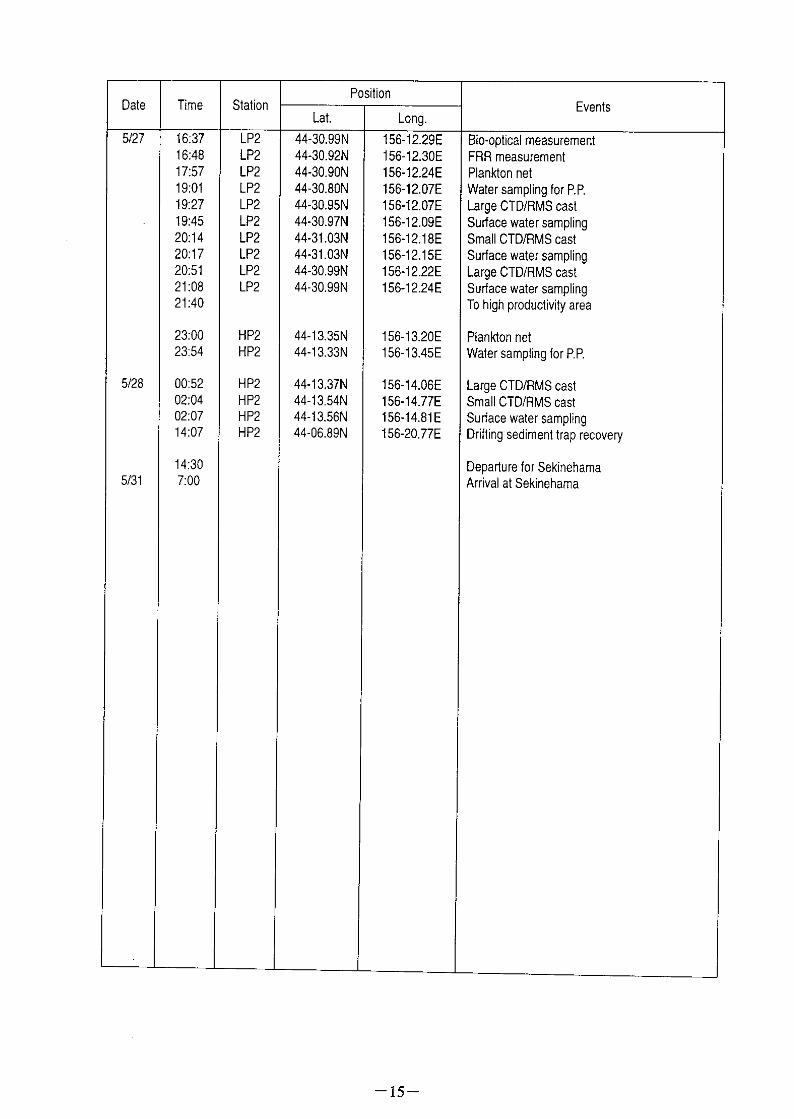
2.2 Cruise track and cruise log ------------------------------------------------------------------- 10
2.3 List of participants ---------------------------------------------------------------------------- 16
3. Observation
3.1 Meteorological measurement ---------------------------------------------------------------- 18
3.2 Temperature and salinity measurement / water sampling by CTD / RMS --------------- 27
3.3 Dissolved oxygen, nutrients, and salinity
3.3.1 Dissolved oxygen ---------------------------------------------------------------- 30
3.3.2 Nutrients measurements of sea water sample -------------------------------- 35
3.3.3 Salinity measurement ----------------------------------------------------------- 38
3.4 Carbonate chemistry
3.4.1 pH ---------------------------------------------------------------------------------- 40
3.4.2 Total dissolved inorganic carbon ---------------------------------------------- 50
3.4.3 Total alkalinity ------------------------------------------------------------------- 52
3.4.4 Carbon isotopes ------------------------------------------------------------------ 53
3.4.5 Study of carbon system at the station KNOT -------------------------------- 54
3.4.6 Dissolved organic carbon ------------------------------------------------------- 55
3.4.7 Water sampling for analysis of long-chain unsaturated alkenones -------- 56
3.5 Particulate organic carbon (POC) ---------------------------------------------------------- 59
3.6 Phytoplankton pigment
3.6.1 Phytoplankton pigment measurements in the subarctic North Pacific ------ 60
3.6.2 Phytoplankton pigments -------------------------------------------------------- 66
3.7 Trace metal: behavior of iron in the Northwestern North Pacific ocean -------------- 67
3.8 Gas
3.8.1 Halocarbon ----------------------------------------------------------------------- 71
3.8.2 Measurement of halogenated volatile organic confounds ----------------- 72
3.9 Water collection for TFA ---------------------------------------------------------------------- 73
3.10 Radionuclides
3.10.1 234Th by JAMSTEC ---------------------------------------------------------- 75
3.10.2 Time-series observation of 234Th, 210Po and 210Pb at KNOT station -- 76
3.11 Primary production ---------------------------------------------------------------------------- 78
3.12 Drifting sediment trap experiment -------------------------------------------------------- 81
3.13 Time-series sediment trap experiment ------------------------------------------------ 101
3.14 Bio-optical measurements in the subarctic North Pacific ocean
for ocean color remote sensing ----------------------------------------------------- 115
3.15 Plankton ------------------------------------------------------------------------------------ 117
3.16 Atmospheric observation
3.16.1 Atmospheric input of iron over the northwestern North Pacific ocean - 120
3.16.2 Atmospheric aerosol and ozone in the marine boundary layer -------- 123
3.16.3 Nonmethane hydrocarbons and ozone measurements over the western
North Pacific ------------------------------------------------------------------------- 128
3.16.4 Organic aerosols over the western North Pacific ----------------------- 129
3.17 Underway observation
3.17.1 Partial pressure of CO2 (pCO2) in the atmosphere and sea surface --- 131
3.17.2 Measurement of CO2 in the atmosphere and in surface seawater --- 132
3.17.3 Salinity, temperature, DO, and Fluorescence -------------------------- 133
3.17.4 Nutrients monitoring in sea water --------------------------------------- 144
3.18 Sea floor sediment sampling and study on geochemical cycle on sea floor ------- 146
3.19 ADCP ------------------------------------------------------------------------------------- 151
3.20 Underway geophysics
3.20.1 Multi-narrow beam echo sounding system ------------------------------- 158
3.20.2 Sea surface gravity -------------------------------------------------------- 166
3.20.3 Surface three component magnetometer ------------------------------- 167
Appendix
1. Vertical profiles for temperature, salinity, DO and fluorescence ------------------- A- 1
2. CTD bottle list and routine data --------------------------------------------------------- A-43
3. Seawater surface temperature observed by satelite NOAA
(AVHRR data compiled by Sasaoka of Hokkaido Univ.) -------------------- A-88
1. Preface
Makio Honda (Principle Investigator)
R/V MIRAI left her mother port Sekinehama on 8 May, 1999 for MR99-K02 cruise. The
principle objective of this cruise was the study of biogeochemistry under the "spring bloom" condition
expected to occur in the northwestern North Pacific in this season. We visited three main stations and
conducted the comprehensive observations including hydrocasts, sea floor sediment coring, moored
and drifting sediment trap experiment, plankton net, and aerosol sampling. Every work was carried
out smoothly and successfully. Especially it was the first time to deploy and recover the drifting
sediment trap mooring system with primary production incubation bottles at the mid night. The
enthusiastic work by crew members enabled us to conduct this work.
On the other hand, it was tough to meet the spring bloom. Although we expected that the
spring bloom would occur at the main stations, we could not meet this phenomena. We carried out
time consuming sea surface monitoring around stn. KNOT to find it. Even if we found that, the water
mass in which the spring bloom might take place moved away and we could not return the same water
mass. We felt the importance of real time ocean color data by satellite which was not available this
cruise. Although there was the above difficulty, we succeeded to carry out the comprehensive
observation under the spring bloom condition: color of sea water was brown, sea water pCO2 was
significantly low (< 220 ppm) and concentrations of proxy for biological activity such as fluorescence
was high. According to the preliminary report, settling particles collected by drifting sediment traps
or some chemical substances such as halocarbon was significantly higher under the spring bloom
condition.
I thank all of participants for the cooperative research. I hope that the result of observation
will be helpful for our science. I acknowledge marine technicians from Marine Works Japan Inc. and
Global Ocean Development Inc. Without their assist and techniques in chemical analysis, deck works
and sea-beam topography survey and so on, any works were not possible. Finally, I appreciate
captain Akamine, chief engineer Watanabe, chief officer Kurihara, and crew members. Although we
participants might force them to work for 24 hours and drive the MIRAI along the transect which was
not planned and we decided suddenly on board, they worked devotedly and satisfied our request.
2. Outline of MR99-K02 2.1 Cruise summary Makio Honda (Principle Investigator)
(Japan Marine Science and Technology Center) The main objective of MR99-K02 cruise (from 8 May to 1 June, 1999) by R/V "MIRAI" was
the study of material cycle under the "spring bloom" condition in the northwestern North Pacific. We
visited three stations with emphesis on the observation at stn. KNOT, which is the Japanese time series
station for the biogeochemical study. We visited stn. KNOT twice at the begining and late of cruise
in order to observe the change in marine chemistry and biology during the "spring bloom" and
conducted the comprehensive observations as follows:
(1) Underway observation of pCO2, TCO2, nutrients, DO, fluorescence
(2) Hydrocasting for Sal., DO, nutrients, pH, pCO2, TCO2, TALK, carbon isotopes, chl-a,
halocarbon, POC, and radionuclide
(3) Sea floor sediment sampling by mu ltiple corer
(4) Drifting sediment trap experiment
(5) Primary productivity measurement by in-situ and quasi in-situ method (on deck incuvation)
(6) Plankton sampling
(7) Recover and re-deployment of moored sediment trap system
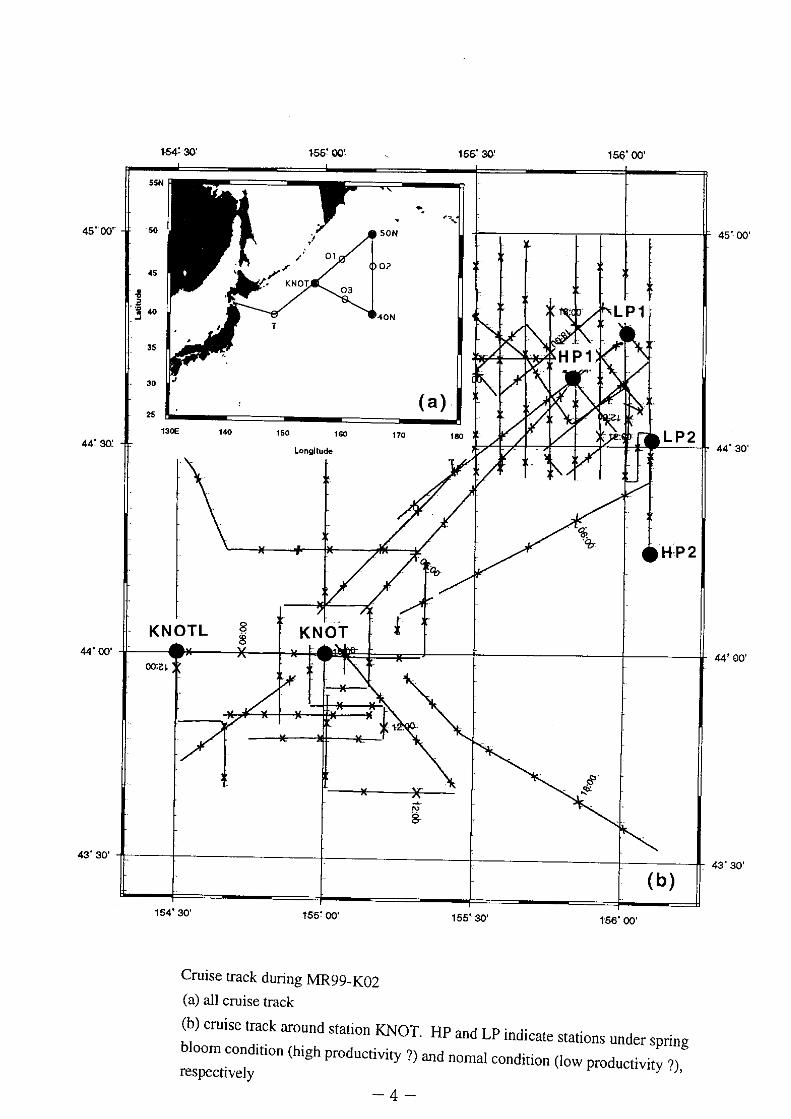
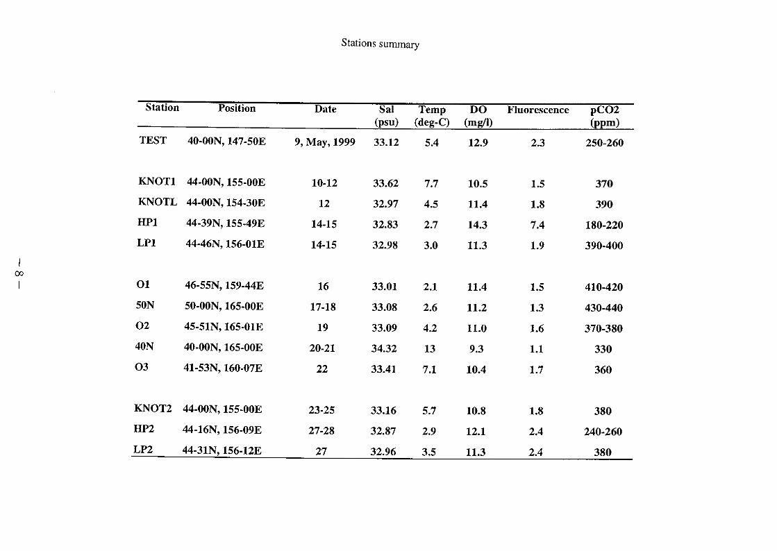
When we visited stn. KNOT, the " spring bloom" had not taken place yet. Stn. KNOT was
located at the "sub-arctic boundary" and was unusually covered with the "Kuroshio " related water
judging from high temperature (> 7 °C) and salinity (> 33 psu). Collected materials by the mo ored
sediment traps which recovered at stn. KNOT also showed that the spring bloom has not taken place
yet. Although we investigated the "spring bloom" around stn. KNOT, we could not find the "spring
bloom" event. We conducted the comprehensive observation under the above condition at stn.
KNOT.
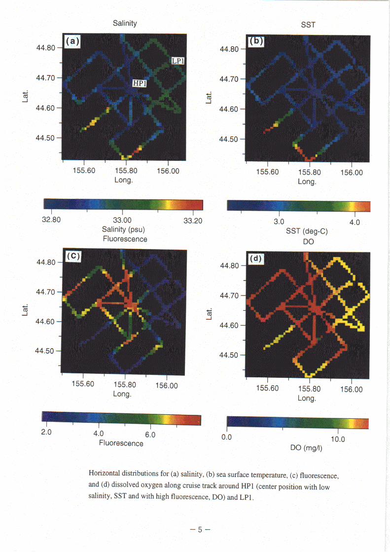
However, on the way to stn. 50N, approximately 40 nautical miles northeastward from stn.
KNOT, we met the water mass where sea-water pCO2 was about 200 ppm and concentration of
fluorescene was 4 times higher than that at stn. KNOT and color of sea water was brown. We quickly
changed our schedule and conducted the comprehensive observation at this position named "stn.
HP1". It is noteworthy that the properties of water was changable and it was hard to say that we
could conduct all observations in the same water mass perfectly.

Unfortunately, we did not meet the "spring bloom" at the second visit to stn KNOT either.
After we conducted the basic observation at stn. KNOT , we made a big effort to find the "spring
bloom" around stn. HP1. However we did not find the "spring bloom" event which we met before.
Instead of the "spring bloom" area, we conducted the observation in the area, named stn. HP2, where
sea water pCO2 was relatively lower (approximately 250 ppm) and fluorescene was higher than stn.
KNOT.
Most of results of the above observations should be waited until the analysis on land is
completed. However the following interesting things has been reported on board:
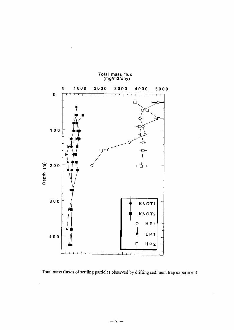
(a) Qualitatively speaking, settling particles collected by floating sediment trap were largely higher at
stn. HP1 and HP2 than stn. KNOT and other stations.
(b) Concentrations of halocarbon and DMS which suspected to be produced by phytoplankton was two
times higher at stn. HP.
(c) Nutrients were relatively consumed up.
Beside the above bloom study, we also carried out the observation at stn. 50N and 40N. As
same as stn. KNOT, we did not observe any phenomena attributed to the "spring bloom". At both
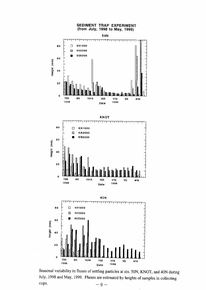
stations, moored sediment trap systems which deployed last July, 1998, were recoverd successufully.
High flux of settling particles could be seen in the middle of the last April, 1999, at stn. 50N.
However it was difficult to define this high flux as the "spring bloom" because sea water pCO2
was
still equal to or slightly higher than atmospheric pCO2. It is likely that the real "spring bloom" which
lowers sea water pCO2 is comming after our cruise.

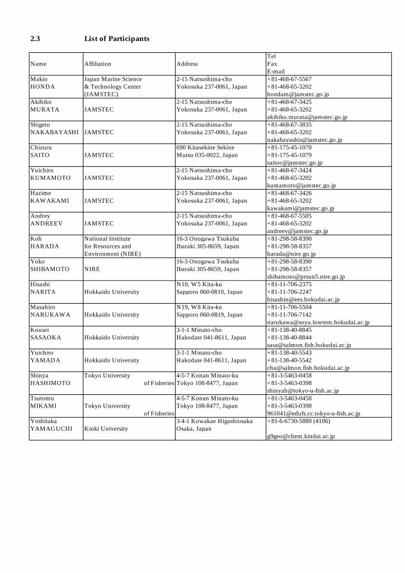
2.3 List of Participants
TelName Affiliation Address Fax
E-mailMakio Japan Marine Science 2-15 Natsushima-cho +81-468-67-5567HONDA & Technology Center Yokosuka 237-0061, Japan +81-468-65-3202
(JAMSTEC) [email protected] 2-15 Natsushima-cho +81-468-67-3425MURATA JAMSTEC Yokosuka 237-0061, Japan +81-468-65-3202
[email protected] 2-15 Natsushima-cho +81-468-67-3835NAKABAYASHI JAMSTEC Yokosuka 237-0061, Japan +81-468-65-3202
[email protected] 690 Kitasekine Sekine +81-175-45-1070SAITO JAMSTEC Mutsu 035-0022, Japan +81-175-45-1079
[email protected] 2-15 Natsushima-cho +81-468-67-3424KUMAMOTO JAMSTEC Yokosuka 237-0061, Japan +81-468-65-3202
[email protected] 2-15 Natsushima-cho +81-468-67-3426KAWAKAMI JAMSTEC Yokosuka 237-0061, Japan +81-468-65-3202
[email protected] 2-15 Natsushima-cho +81-468-67-5505ANDREEV JAMSTEC Yokosuka 237-0061, Japan +81-468-65-3202
[email protected] National Institute 16-3 Onogawa Tsukuba +81-298-58-8390HARADA for Resources and Ibaraki 305-8659, Japan +81-298-58-8357
Environment (NIRE) [email protected] 16-3 Onogawa Tsukuba +81-298-58-8390SHIBAMOTO NIRE Ibaraki 305-8659, Japan +81-298-58-8357
[email protected] N10, W5 Kita-ku +81-11-706-2375NARITA Hokkaido University Sapporo 060-0810, Japan +81-11-706-2247
[email protected] N19, W8 Kita-ku +81-11-706-5504NARUKAWA Hokkaido University Sapporo 060-0819, Japan +81-11-706-7142
[email protected] 3-1-1 Minato-cho +81-138-40-8845SASAOKA Hokkaido University Hakodate 041-8611, Japan +81-138-40-8844
[email protected] 3-1-1 Minato-cho +81-138-40-5543YAMADA Hokkaido University Hakodate 041-8611, Japan +81-138-40-5542
[email protected] Tokyo University 4-5-7 Konan Minato-ku +81-3-5463-0458HASHIMOTO of Fisheries Tokyo 108-8477, Japan +81-3-5463-0398
[email protected] 4-5-7 Konan Minato-ku +81-3-5463-0458MIKAMI Tokyo University Tokyo 108-8477, Japan +81-3-5463-0398
of Fisheries [email protected] 3-4-1 Kowakae Higashiosaka +81-6-6730-5880 (4106)YAMAGUCHI Kinki University Osaka, Japan
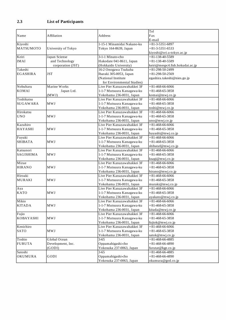
2.3 List of Participants
TelName Affiliation Address Fax
E-mailKiyoshi 1-15-1 Minamidai Nakano-ku +81-3-5351-6897MATSUMOTO University of Tokyo Tokyo 164-8639, Japan +81-3-5351-6533
[email protected] Japan Sciense 3-1-1 Minato-cho +81-138-40-5589IMAI and Technology Hakodate 041-8611, Japan +81-138-40-5589
corporation (JST) (Hokkaido University) [email protected] 16-2 Onogawa Tsukuba +81-298-50-2499EGASHIRA JST Ibaraki 305-0053, Japan +81-298-50-2569
(National Institute [email protected] for Environmental Studies)
Nobuharu Marine Works Live Pier Kanazawahakkei 3F +81-468-66-6066KOMAI Japan Ltd. 1-1-7 Mutsuura Kanagawa-ku +81-468-65-3858
(MWJ) Yokohama 236-0031, Japan [email protected] Live Pier Kanazawahakkei 3F +81-468-66-6066SUGAWARA MWJ 1-1-7 Mutsuura Kanagawa-ku +81-468-65-3858
Yokohama 236-0031, Japan [email protected] Live Pier Kanazawahakkei 3F +81-468-66-6066UNO MWJ 1-1-7 Mutsuura Kanagawa-ku +81-468-65-3858
Yokohama 236-0031, Japan [email protected] Live Pier Kanazawahakkei 3F +81-468-66-6066HAYASHI MWJ 1-1-7 Mutsuura Kanagawa-ku +81-468-65-3858
Yokohama 236-0031, Japan [email protected] Live Pier Kanazawahakkei 3F +81-468-66-6066SHIBATA MWJ 1-1-7 Mutsuura Kanagawa-ku +81-468-65-3858
Yokohama 236-0031, Japan [email protected] Live Pier Kanazawahakkei 3F +81-468-66-6066SAGISHIMA MWJ 1-1-7 Mutsuura Kanagawa-ku +81-468-65-3858
Yokohama 236-0031, Japan [email protected] Live Pier Kanazawahakkei 3F +81-468-66-6066HIRANO MWJ 1-1-7 Mutsuura Kanagawa-ku +81-468-65-3858
Yokohama 236-0031, Japan [email protected] Live Pier Kanazawahakkei 3F +81-468-66-6066MURAKI MWJ 1-1-7 Mutsuura Kanagawa-ku +81-468-65-3858
Yokohama 236-0031, Japan [email protected] Live Pier Kanazawahakkei 3F +81-468-66-6066KATO MWJ 1-1-7 Mutsuura Kanagawa-ku +81-468-65-3858
Yokohama 236-0031, Japan [email protected] Live Pier Kanazawahakkei 3F +81-468-66-6066KITADA MWJ 1-1-7 Mutsuura Kanagawa-ku +81-468-65-3858
Yokohama 236-0031, Japan [email protected] Live Pier Kanazawahakkei 3F +81-468-66-6066KOBAYASHI MWJ 1-1-7 Mutsuura Kanagawa-ku +81-468-65-3858
Yokohama 236-0031, Japan [email protected] Live Pier Kanazawahakkei 3F +81-468-66-6066SATO MWJ 1-1-7 Mutsuura Kanagawa-ku +81-468-65-3858
Yokohama 236-0031, Japan [email protected] Global Ocean 3-65 +81-468-66-4885FURUTA Development, Inc. Oppamahigashi-cho +81-468-66-4890
(GODI) Yokosuka 237-0063, Japan [email protected] 3-65 +81-468-66-4885OKUMURA GODI Oppamahigashi-cho +81-468-66-4890
Yokosuka 237-0063, Japan [email protected]
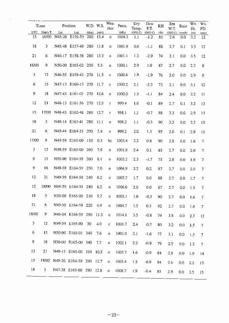
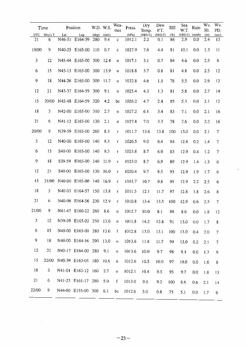
3. Observation 3.1 Meteorological measurement
Satoshi Okumura
(Global Ocean Development Inc.)
(1) Introduction
Some surface meteorological parameters were observed throughout R/V Mirai MR99-K02
Cruise from the departure of Sekinehama on May 8 to the return to Sekinehama on May 31, 1999.
Parameters of these observations are as follows:
Press.: Atmospheric pressure adjusted to the sea surface level [hPa]
D r y A i r T e m p . : A t m o s p h e r i c d r y t e m p e r a t u r e [ d e g - C ]
W e t A i r T e m p . : A t m o s p h e r i c w e t t e m p e r a t u r e [ d e g - C ]
D e w P . T . : D e w p o i n t t e m p e r a t u r e [ d e g -C ]
R H : R e l a t i v e h u m i d i t y [ % ]
R a i n : P r e v i o u s 1 h o u r p r e c i p i t a t i o n [ m m ]
W . D . : 1 0 m i n u t e s a v e r a g e d w i n d d i r e c t i o n [ d e g ]
W . S . : 1 0 m i n u t e s a v e r a g e d w i n d s p e e d [ m / s ]
S S T : S e a s u r f a c e t e m p e r a t u r e [ d e g - C ]
W v . H t : S i g n i f i c a n t w a v e h e i g h t m e a s u r e d f i r s t 2 0 m i n u t e s a t e v e r y 3
h o u r s ( 0 2 0 0 , 0 5 0 0 , 0 8 0 0 , 1 1 0 0 , 1 4 0 0 , 1 7 0 0 , 2 0 0 0 , 2 3 0 0 U T C ) [ m ]
W v . P D : P e r i o d o f W v . H t [ s e c ]
R a d i a t i o n : S h o r t a n d l o n g w a v e r a d i a t i o n f r o m s o l a r u p w a r d
l o o k i n g r a d i o m e t e r [ M J / m 2 ]
W e a t h e r : W e a t h e r
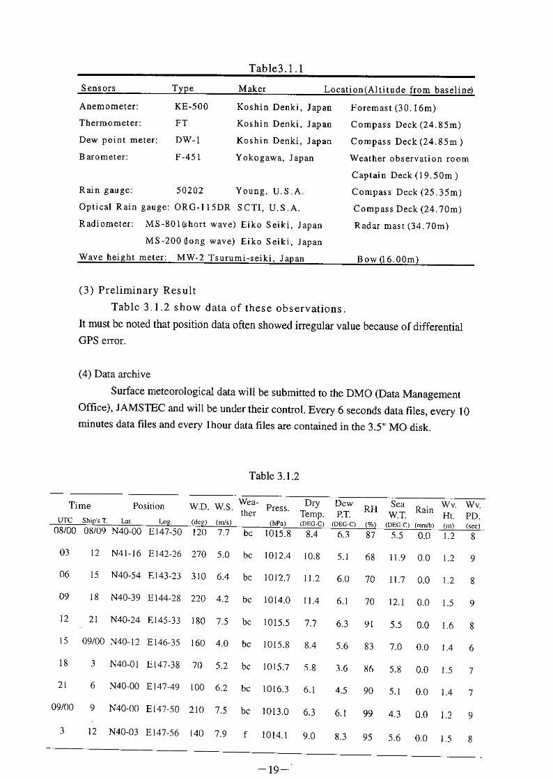
(2) M e t h o d s
S u r f a c e m e t e o r o l o g i c a l d a t a w e r e c o l l e c t e d a n d p r o c e s s e d b y K O A C - 7 8 0 0 w e a t h e r d a t a p r o c e s s o r a
n d s o m e s e n s o r s a s s e m b l e d b y K o s h i n D e n k i , J a p a n . T h e R / V M i r a i o n b o a r d s e n s o r s f o r m e t e o r o l o g i c a l m e
a s u r e m e n t s a r e l i s t e d b e l o w .


3. 2 Temperature and Salinity measurement / Water sampling by CTD / RMS
Hirokatsu UNO, Fujio KOBAYASHI, Mizue HIRANO
(Marine Works Japan Ltd.)
Chizuru SAITO, Makio HONDA
(Japan Marine Science and Technology Center)
(1) Introduction
As a basic property of the water mass in the study area, temperature and salinity were measured
by CTD, and sea water sampling was conducted by RMS in order to obtain the samples for chemical
analysis. In this section, we describe as for the CTD/RMS observations in MR99-K02 cruise conducted
from 8 May 1999 to 31 May 1999 by R/V MIRAI.
(2) Measured Items
Temperature and Salinity were measured from sea surface through 5,300m in maximum (Large
system) or 3,500m in maximum (Small system), and sea waters were sampled at stations KNOT, 50N,
40N and other stations by using CTD(conductivity-temperature-depth profiler) / RMS (Rosette
Multi-bottle array water sampling Systems). CTD/RMS water-sampling casts of 2-14 times were
conducted at every station (51 casts in total) for the chemical analysis of general water properties, carbon,
trace metals, radio isotope, etc. .
(3) Observation Methods
(a) CTD/RMS systems
Two CTD/Rosette Multi-bottle Array Systems (CTD/RMS) were used during this cruise. One
was the 30-liters 24-positions intelligent General Oceanic RMS (GO 1016) water sampler with Sea-Bird
Electronics, Inc. CTD (SBE911plus) for 10,500 meters, nicknamed Large-CTD/RMS. Another one was
the same CTD and RMS as Large CTD/RMS, but with 12-liters 12-positions water sampler, nicknamed
Small-CTD/RMS.
30-liters and 12-liters Niskin bottles were attached on each Rosette system, 12 bottles of which
were especially cleaned for the trace metal analysis. The sensors attached on each CTD were
temperature sensor, conductivity sensor, pressure sensor and altimeter. In addition, Large-CTD/RMS was
also with DO sensor and Fluorometer (Fluorometer . The calibration of these sensors were conducted by
SBE in May 1994. Specification of the sensors were listed below.
CTD/RMS Sensor Model Serial No.
Large-CTD/RMS
Temperature SBE3-04/F Primary S/N031524
Conductivity SBE4-04/O Primary S/N041203
Pressure S/N 42410
Oxygen SBE13-04 S/N130338
Altimeter Benthos2110-1 S/N 0206
Fluormeter S/N 2148
Small-CTD/RMS
Temperature SBE3-04/F Primary S/N031359
Conductivity SBE4-04/O Primary S/N041202
Pressure S/N 42423
Altimeter Benthos2110-1 S/N 0205
(b) Operation during Observation
Large-CTD/RMS was deployed and recovered from the stern of R/V MIRAI using the A-frame,
and another small frame installed on starboard side, named as the Gallows, was used for
Small-CTD/RMS. The CTD raw data was acquired on real time by using a SEASAVE utility of a
software SEASOFT (Ver. 4.232) provided by Sea-Bird Electronics, Inc. and stored on the hard disk of a
personal computer set in After Wheel-house. Water samplings were made during up cast by sending a
fire command from the computer. Detail information during a cast such as date/time, station/cast/file
names, location at the start/bottom/end of observation, water sampling layers and events were recorded in
a CTD cast log sheet. These were summarized in CTD Cast List or CTD Bottle List shown in
Appendix.
After a cast, the Large-CTD/RMS was lifted down from upper deck to the Water Drawing Room on 2nd
deck and sea water was drawn from the bottles.
(c) CTD data processing
The CTD raw data was processed by using SEASOFT (Ver. 4.232) on another computer (IBM
PS/V). Procedure of the data processing and used utilit ies of SEASOFT were as following.
DATCNV: Converts the binary raw data to output on physical units. Output items are depth,
pressure, potential temperature, salinity, density(sigma-theta), oxygen, fluorescence.
Simultaneously, this utility selects the CTD data when bottles closed to output on another file.
WILDEDIT: Marks wild points by setting their values to the bad value specified in the input .CNV
header. The first pass of WILDEDIT is used to obtain an accurate estimate of the true standard
deviation of the data. The second pass is used to mark the values good or bad.
SPLIT: Splits the data made by DATCNV into up and down cast data.
BINAVG: Calculates the averaged data in every 1 meter.
ASCIIOUT: Converts the binary averaged data into ASCII format data.
ROSSUM: Edits the data of sampled water to output a summary file. These data were shown
in tables in Appendix CTD Bottle List.
SEAPLOT: Display the vertical profiles of averaged potential temperature, salinity, sigma-theta,
oxygen ,and fluorescence data on CRT and print out. Plotted profiles for every station are
shown in Figures in appendix.
(4) Management of the CTD data
A file name of each cast consist of the cruise identification, station name, CTD/RMS type and
cast number, e.g., 99K2K1L1. After SPLIT utility was used, up/down identification was added. As a
result of above on-board processing, 12 files were made for 1 cast, such
as .DAT, .CON, .HDR, .BL, .ROS, .BTL, d*.CNV, u*.CNV, d*.ASC, u*.ASC, d*.HDR, u*.HDR files.
All of raw and processed CTD data files were copied into a 3.5 inch magnetic optical disk (MO disk).
3. 3 Dissolved oxygen, nutrients and salinity 3 . 3 . 1 Dissolved oxygen
N o b u h a r u K o m a i , K a t s u n o r i S a g i s h i m a
( M a r i n e W o r k s J a p a n L t d . )
C h i z u r u S a i t o
( J a p a n M a r i n e S c i e n c e a n d T e c h n o l o g y C e n t e r )
( 1 ) I n t r o d u c t i o n
D i s s o l v e d o x y g e n i s a m a j o r p a r a m e t e r f o r d e c i d i n g t h e s e a w a t e r c h a r a c t e r i s t i c o n o c e a n o g r a p h y. In
this cruise, the methods of dissolved oxygen determination is based on WHP Operations and Methods
manual (Culberson, 1991, Dickson, 1994).
(2) Methods
(a) Instruments and Apparatus
Glass bottle : Glass bottle for D.O. measurements consist of the ordinary BOD
flask (ca.180ml) and glass stopper with long nipple, modified
from the nipple presented in Green and Carritt (1966).
Dispenser : Eppendorf Comforpette 4800 / 1000µl
O P T I F I X / 2 m l ( f o r M n C l 2
& N a O H / N a I a q . )
M e t r o h m M o d e l 7 2 5 M u l t i D o s i m a t / 2 0 m l ( f o r K I O3 )
T i t r a t o r : M e t r o m M o d e l 7 1 6 D M S T i t r i n o / 1 0 m l o f t i t r a t i o n
v e s s e l
M e t r o m P t E l e c t r o d e / 6 . 0 4 0 3 . 1 0 0 ( N C )
S o f t w a r e : D a t a acquisition and endpoint evaluation / Metrohm,
METRODATA / 606013.000
(b) Methods
Sampling and analytical methods were based on to the WHP Operations and Methods
(Culberson, 1991, Dickson, 1994) .
(b-1) Sampling
Seawater samples for dissolved oxygen measurement were collected from 30 L Niskin bottles to
calibrated dry glass bottles. During each sampling, 3 bottle volumes of seawater sample were overflowed
to minimize contamination with atmospheric oxygen and the seawater temperature at the time of
collection was measured for correction of the sample volume.
After the sampling, MnC l 2
(aq.) 1ml and NaOH/NaI (aq.) 1ml were added into the glass bottle, and
then shook the bottle well. After the precipitation has settled, we shook the bottle vigorously to disperse
the precipitate.
(b-2) D.O. analysis
The samples were analyzed by 2 sets of Metrohm titrators with 10 ml piston buret and Pt
Electrode using whole bottle titration. Titration was determined by the potentiometric methods and the
endpoint for titration was evaluated by the software of Metrohm, METRODATA (606013.000).
Concentration of D.O. was calculated by equation (8) and (9) of WHP Operations and Methods
(Culberson, 1991). Salinity value of the equation (9) was used from the value of salinity of CTD. The
amount of D.O. in the reagents was reported 0.0017 ml at 25.5 deg-C (Murray et al., 1968). However in
this cruise, we used the value (= 0.0027 ml at 21 deg-C) measured at 1995 WOCE cruise of R/V Kaiyo.
D.O. concentrations we calculated were not corrected by seawater blank.
We prepared and used one batch of 5 liter of 0.07N thiosulfate solutions and 5 liter of 0.0100N
standard K I O3 solutions (JM981130). The standardizations and blank determination have been
performed every day before the sample analysis. The value of thiosulfate standardization of titrator #A
was significantly changed at 20-May-99, so we didnít use a titrator #A since that day.
(3) Preliminary Result
(3-1) Comparison of our K I O3
standards to CSK standard solution.
After this cruise, we compared our standards with CSK standard solution (Lot. DLG8365) which
is the commercially available standard solution prepared by Wako Pure Chemical Industries, Ltd. The
results are shown in table 3.3.1-1. Normality of our standard may be different 0.02% from nominal
normality.
Table 3.3.1-1. Comparison of each standards
K I O3
Lot No. Nominal Average Standard n Ratio to
Normality Titer (ml) Deviation DLG8365 (CSK)
DLG 8365 0.0100 1.3826 0.0005 10
JM981016 0.010019 1.3950 0.0007 10 0.9998
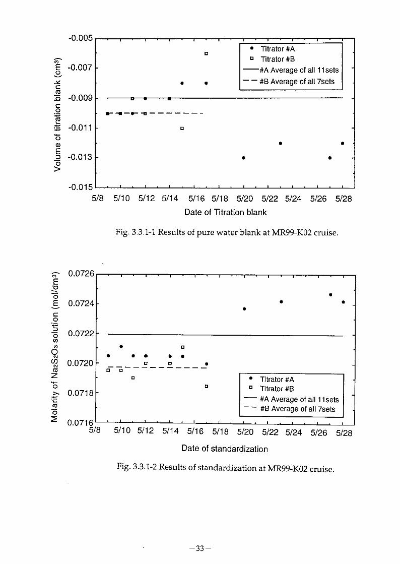
(3-2) Titration blanks
The titration blank were determined in deionized water by Milli-RX12, Millipore. The blank
results from the presence of redox species apart from oxygen in the reagents which can behave
equivalently to oxygen in the analysis. The results were shown in Fig.3.3.1-1. The average of titiration
blank was -0.010 ml (Titrator #A) and -0.009 ml (Titrator #B), respectively.
(3-3) Thiosulfate Standardization
The results of standardization were shown in Fig.3.3.1-2. The average of molarity of thiosulfate
solution was 0.07219 mol (Titrator #A) and 0.07197 mol (Titrator #B) with standard deviation was
0.00019 mol and 0.00008 mol, respectively. Molarity of titrator #A was high since 20-May-99 when the
room temperature was high (ca.28 deg-C).
(3-4) Reproducibility
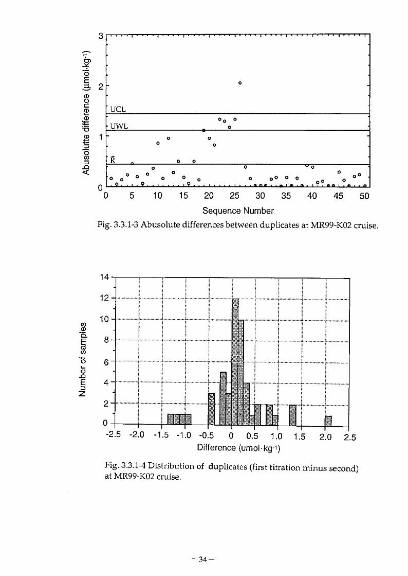
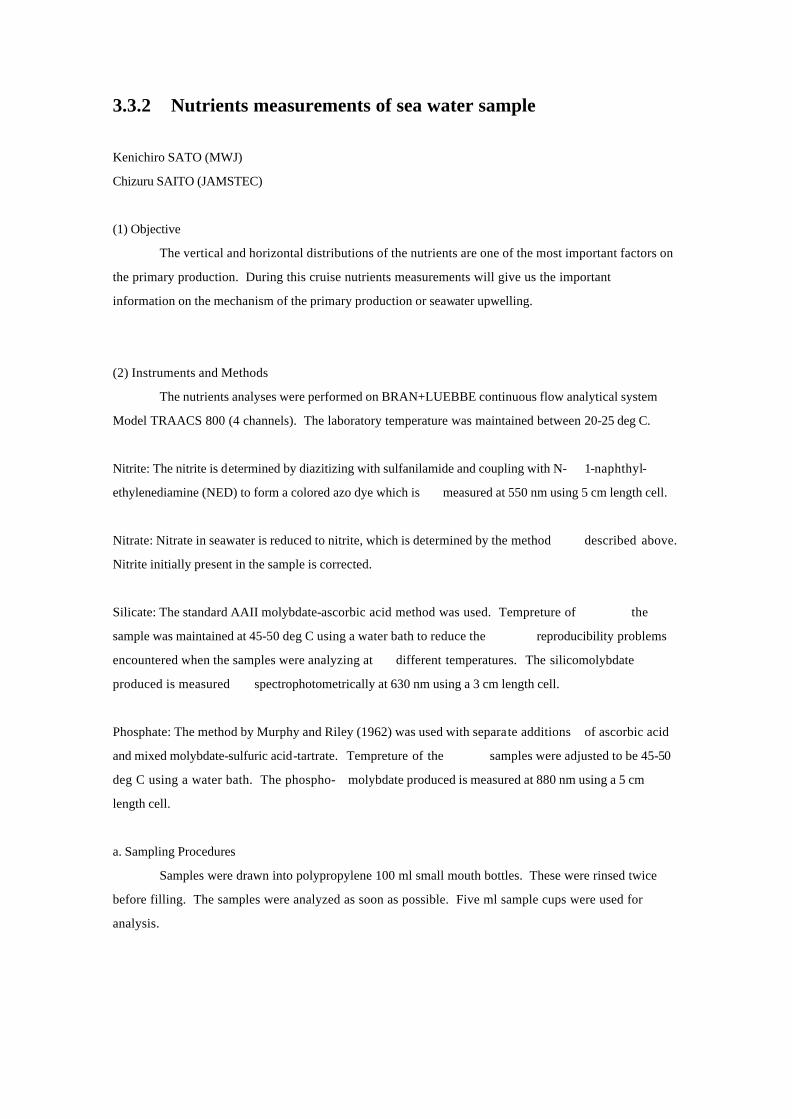
In this cruise, 324 samples for D.O. samples were collected. 50 pairs (15%) of total samples
were analyzed as "duplicates" which were collected from same Niskin bottle. These results were shown in
Fig. 3.3.1-3 and 3.3-1-4. At Fig. 3.3.1-3, absolute difference of the samples whose sequence number 19 to
26 was high. These samples were collected at Stn. 50, so the precision of the collected samples at Stn.
50N seemed to be not good.
From duplicate analyses, the precision of this analysis was evaluated to be 0.44 µmol/kg (one
sigma). This is corresponded to 0.11% of D.O. maximum concentration 411.86 µmol/kg observed in this
cruise.
(4) References :
Culberson, C.H. (1991) Dissolved Oxygen, in WHP Operations and Methods, Woods Hole., pp1-15
Culberson, C.H., G.Knapp, R.T.Williams and F.Zemlyak (1991) A comparison of methods for the
determination of dissolved oxygen in seawater. (WHPO 91-2)
Dickson, A.G. (1994) Determination of dissolved oxygen in sea water by Winkler titration, in WHP
Operations and Methods, Woods Hole., pp1-14.
Green, E.J. and D.E. Carritt (1966) An Improved Iodine Determination Flask for Whole-bottle Titrations,
Analyst, 91, 207-208.
Murray, N., J.P. Riley and T.R.S. Wilson (1968) The solubility of oxygen in Winkler reagents used for
the determination of dissolved oxygen, Deep-Sea Res., 15, 237-238.
3.3.2 Nutrients measurements of sea water sample
Kenichiro SATO (MWJ)
Chizuru SAITO (JAMSTEC)
(1) Objective
The vertical and horizontal distributions of the nutrients are one of the most important factors on
the primary production. During this cruise nutrients measurements will give us the important
information on the mechanism of the primary production or seawater upwelling.
(2) Instruments and Methods
The nutrients analyses were performed on BRAN+LUEBBE continuous flow analytical system
Model TRAACS 800 (4 channels). The laboratory temperature was maintained between 20-25 deg C.
Nitrite: The nitrite is determined by diazitizing with sulfanilamide and coupling with N- 1-naphthyl-
ethylenediamine (NED) to form a colored azo dye which is measured at 550 nm using 5 cm length cell.
Nitrate: Nitrate in seawater is reduced to nitrite, which is determined by the method described above.
Nitrite initially present in the sample is corrected.
Silicate: The standard AAII molybdate-ascorbic acid method was used. Tempreture of the
sample was maintained at 45-50 deg C using a water bath to reduce the reproducibility problems
encountered when the samples were analyzing at different temperatures. The silicomolybdate
produced is measured spectrophotometrically at 630 nm using a 3 cm length cell.
Phosphate: The method by Murphy and Riley (1962) was used with separate additions of ascorbic acid
and mixed molybdate-sulfuric acid-tartrate. Tempreture of the samples were adjusted to be 45-50
deg C using a water bath. The phospho- molybdate produced is measured at 880 nm using a 5 cm
length cell.
a. Sampling Procedures
Samples were drawn into polypropylene 100 ml small mouth bottles. These were rinsed twice
before filling. The samples were analyzed as soon as possible. Five ml sample cups were used for
analysis.
b. Low Nutrients Sea water (LNSW)
Ten containers (20L) of low nutrients sea water were collected in early 1998 at equatorial Pacific
and filtered with 0.45mm pore size membrane filter (Millipore HA). They are used as preparing the
working standard solution.
(3) Preliminary results
a. Precision of the analysis
We have made the repeat analysis of two layers' (about 100 m and 500 m depths) samples at
each station. At those repeat analysis range of CV (concentration average to standard deviation) were
0.03 to 2.6 % in upper layer and 0.07 to 1.9 % in bottom layer except nitrite.
b.Distribution of nutrients
The results are shown in Appendix.
In this expedition we made a hit of spring blooming spot. Surface nutrient concentrations were
extremrely low compared with other season. On the other hand, the highest concentrations were
observed upper 1000 m layer in stn. 50N. Anyway we are looking forward to analyzing the blooming
season's data.
These data are stored in MO disk in Ocean Research Department in JAMSTEC.


3. 3. 3 Salinitiy measurements
Hirokatsu UNO, Fujio KOBAYASHI, Mizue HIRANO
(Marine Works Japan Ltd.)
Chizuru SAITO
(Japan Marine Science and Technology Center)
(1) Instrument and Method
Salinity was measured by a Guildline Autosal salinometer model 8400B, which was modified by
addition of an Ocean Science International peristalitic-type sample intake pump and Hewlett Packard
quartz thermometer model 2804A with two 18111A quartz probes. One probes measured at room
temperature and the other probe measure at a bath temperature. The resolution of the quartz thermometer
was set to 0.001 °C. Data of both the salinometer and the thermometer was collected simultaneously by a
personal computer. A double conductivtiy ratio was defined as median of 31 times readings of the
salinometer. Data collection started after 5 seconds and it took about 10 seconds to collect 31 reading
by a personal computer.
The salinometer was operated in the air-conditioned ship's laboratory at bath temperature of 24°C.
Room temperature varied from approximately 24°C to 26°C, while a variation of bath temperature was
1. Salinity Sample Bottles
The bottles in which the salinity samples are collected and stored are 250 ml brown glass bottles
with screw caps.
2. Salinity Sample Collection and Temperature Equilibration
Each bottles was rinsed twice with sample water and was filled to the shoulder of the bottle. Its
cap was also thoroughly rinsed. Salinity samples were stored more than 24 hours in same laboratory were
the salinity measurement was made.
3. Standardization
Autosal model 8400B was standardized before and after sequence of measurements by use of
IAPSO Standard Seawater batch P134 whose conductivity ratios were 0.99989.
4. Sub-Standard Seawater
We also used sub-standard seawater which was deep-sea water filtered by pore size of 0.45
micrometer and stored in a 20 liter container made of polyethylene for at least 24 hours before measuring.
It was measured every 10 samples in older to check and correct the trend.

(2)Result
The result obtained are shown in CTD/RMS bottle lists in Appendix.
These salinity data are stored in Ocean Research Department, JAMSTEC.
3.4 Carbonate chemistry 3.4.1. pH measurements
Andray Andreev (JAMSTEC)
(1) Introduction
The pH (-log [H+]) of the seawater has used to be considered as a key factor which determine the
form of existence and migration of chemical elements in the seawater. Also the change of the carbonate
parameters of the world ocean due to increase of the antropogenic CO2 concentration in the atmosphere
demands the precise measurements of the pH in the seawater.
During last 30 years in the routine expedition work the most popular became the potentiometric
method of the determination of the pH in the seawater by cell with liquid junction or ' salt bridge'
(saturated solution of KCl)
Ag, AgCl | solution of KCL || test solution | H+ - glass - electrode (A).
In such measurements as electrode pair the H+-glass electrode and silver/silver chloride or
mercury/mercury chloride as reference electrode are used to apply.
The calibration of the electrodes of the cell (A) can be done by using phosphate buffer solution
(Na2HPO4 and KH2PO4 in the distilled water) (NBS scale) and in the total hydrogen scale (T) by
TRIS and AMP in the synthetic seawater (Dickson and Goyet, 1996).
And then the pH of the seawater can be determined by following equation
pH= pH(standard)+ F(Es - Et)/RT•ln(10) (1)
, where (Es - Et) is the difference in EMF of standard and test solutions, RT( ln (10)/F is Nernst
constant (59. 16 mv/pH unit at the temperature 25 degree C).
The main problem of the measurement by cell (A) it is problem of the residual liquid junction
potential (LJP) which arise on the interface of ' salt bridge' and test solution (additional term in the
equation 1). The value of LJP is different in the buffer and test solution and it also depends on the sample
mixing speed in the cell and the level of the KCl solution in the reference electrode.
The difference in the LJP in the standard and test solution can be as high as several mV that leads to the
error in the pH about 0.1 pH unit if use for the pH measurements in the seawater as standard NBS buffer
solutions based on distilled water.
Another problem is that the EMF of the cell (A) is determined by activity of hydrogen ion than
concentration. The coefficient between activity and concentration (coefficient of activity) depends on
salinity. As far salinity of the test solutions from the salinity of the standard solution (for the buffer
solutions in the Total hydrogen scale or SeaWater scale (SWS) it is 35 psu) than higher error in the
determination of pH.
To avoid the problem of liquid junction potential (and drift in EMF related with the change of the level of
KCL solution in the reference electrode) two cells can be applied
Ag, AgCl | solution of KCL || test solution | H+ -glass-electrode (B1),
Ag, AgCl | solution of KCL || est solution | Na+ -glass-electrode (B2)
with common reference Ag, AgCl electrode.
The difference in EMF between cell (B1) and cell (B2) is determined by cell without transfer
Na+ -glass-electrode | test solution | H+ -glass-electrode (C).
The pH of the test solution can be calculated from the measured EMF of the cell (C) by the equation
pH= pH(standard)+ F(Es - Et)/RT•ln(10) + log[(mNa)s/(mNa)t] + log[(γH)s/(γH)t +
log[(γNa)s/(γNa)t] (2)
, where (mNa) and (γNa) are molality and activity coefficient of the sodium ion in the standard (s) and
test (t) solutions, (γH)s and (γH)t are the coefficient of activity of the hydrogen ion in the standard and
test solutions.
In the measurements of the pH of the seawater by cell (A) it used to be assumed that log[(γH)s/(γH)t is
equal to 0.
The (mNa) and (γNa) in the seawater can be determined from salinity (S) by equations:
mNa= 13.872( S/(1000-1.00511•S) (3)
and
ln(γNa)= A•I 0.5 + B•I+ C•I 1.5+ D•I 2+ E•I 2.5 (4)
, where ionic strength of seawater (I) is determined by expression
I= 19.9273(S/(1000- 1.00511•S).
At temperature 25 degree C A= -1.1613, B= 1.4272, C= -1.2976, D= 0.7468 and E= -0.1842
(Tishchenko, 1994).
In (Tishchenko et al., 1999) it was proposed conduct calculation of the pH in the seawater based on EMF
measurements of the cell (C) in the conventional scale (pHC)
pHC= -log[aH]
, where aH is the activity of the hydrogen ion.
The value of (paH (-log [H] -log[γH]) + log[γNa]) (equation 2) in the solution of 0.025 M Na2HPO4+
0.025 M NaH2PO4 + 0.5 m NaCl at the temperature 25 degree C is equal to 6.334 (Tishchenko,
1999).

At the temperature 25 degree C
pHCt = 6.334 + F(Es - Et)/RT•ln(10) + log[(mNa)s/(mNa)t] - log(γNa)t (5)
, where Es is EMF of the solution (0.025 M Na2HPO4+ 0.025 M NaH2PO4 + 0.5 m NaCl),
(mNa)t and (γNa)t in the seawater samples can be calculated by equations (3) and (4).
(2) Instruments and standards
The measurements of the pH of the seawater were carried out by potentiometric method in the
closed cells at the temperature 25 degree C (pH25).
The two types of the electrode cells were applied (A) and (B1)+(B2).
The measurement of EMF of the cell (A) was conducted by pH/Ion meter (model PHM95), pH and
Ag/AgCl reference electrode of the ' Radiometer ' company. The temperature of the test solution was
monitored by temperature sensor (Radiometer) within 0.1 degree C.
For the measurement by cell (B1)+(B2) the pH/ISE meter (model 920A), pH (model 91- 01), sodium -
glass (model 84-11) and Ag/AgCl (model 90-01) of the ' Orion' company were applied.
The four different buffer solutions were used as standards. As primary standard the TRIS (0.04 m TRIS +
0.04 m TRISHCL) in synthetic seawater (S=35 psu) (Total hydrogen scale) (pHT=8.089 pH unit at the
t=25 degree C, Dickson and Goyet, 1996) and phosphate (0.025 M Na2HPO4+ 0.025 M KH2PO4) in the
distilled water (NBS scale, pH=6.865 at t= 25 degree C) only for measurement in the cell (A)) were used
for the electrodes calibration. As secondary standard the phosphate (0.025 M Na2HPO4+ 0.025 M
KH2PO4 in the solution of 0.5 m NaCl and AMP* in the synthetic seawater were applied. The use the
latter buffer solution (AMP*) as secondary standard was due to some deviation in the preparation of the
buffer solution from the prescribed in (Dickson and Goyet, 1996).
Recently a new value of pH25T for the TRIS buffer was adopted (8.0936 pH unit) and we used this
value in our calculation. To do comparison with the historical data it should be take into account the
difference between ' old ' (Dickson and Goyet, 1996) and ' new ' (DelValls and Dickson, 1998)
pH25T
value of the TRIS buffer.
(3) Results and Discussion.
Standard deviation or repeatibility (Dickson and Goyet, 1996) of the pH measurements (S) in the
seawater samples by the cell (A), estimated by following expression S=( (Σdi2/2k) (where di is the
difference between the dublicate measurements and k is amount of the dublicate measurements), was
equal to ± 0.064 mv or ± 0.001 pH unit (k=50). The repeatibility of the measurements in the buffer
solutions was about twice higher than standard deviation of the measurements in the water samples.
The drift in the EMF values of cell B1 and B2 was as much as 2-3 mv for the period 2-3 hours as result of
high outflow rate and hence the change of the level of the KCL saturated solution in the Ag/AgCl
reference electrode of the ' Orion ' company.
The reference electrode of the ' Radiometer ' company was more stable with almost zero drift in EMF
during several hours measurement period.
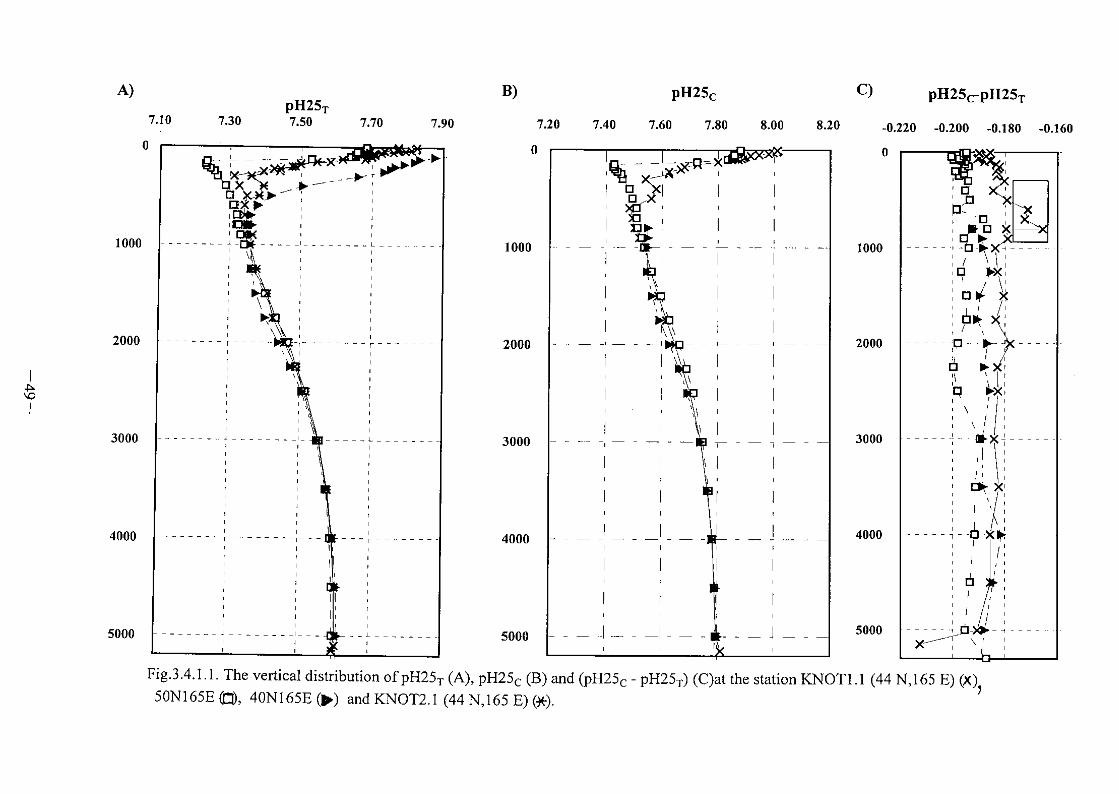
Fig.3.4.1.1 shows the vertical distribution of the pH25T, pH25C and (pH25C - pH25T) at the
deep stations (station KNOT1.1 (44 N, 155 E), 50N165E, 40N165E and KNOT2.1 (44 N, 155 E)
(pH25T)).
In the bottom water layer (depth 4000 - 5500 meters) the distribution of the pH25C at the study stations
was quite uniform (Fig.3.4.1.1). The pH25T was higher at the station 40N165E and it higher at the
station 50N165E.
The average difference between pH25C and pH25T
was equal to -0.188 pH unit, excluding 800-500
meter water layer at the station KNOT1.1. where it was -0.17 pH unit. The low absolute values of the
(pH25C - pH25T) at the shallow hydrocast of the station KNOT1.1 was due to the not proper work of
sodium electrode at the beginning measurements in the cruise.
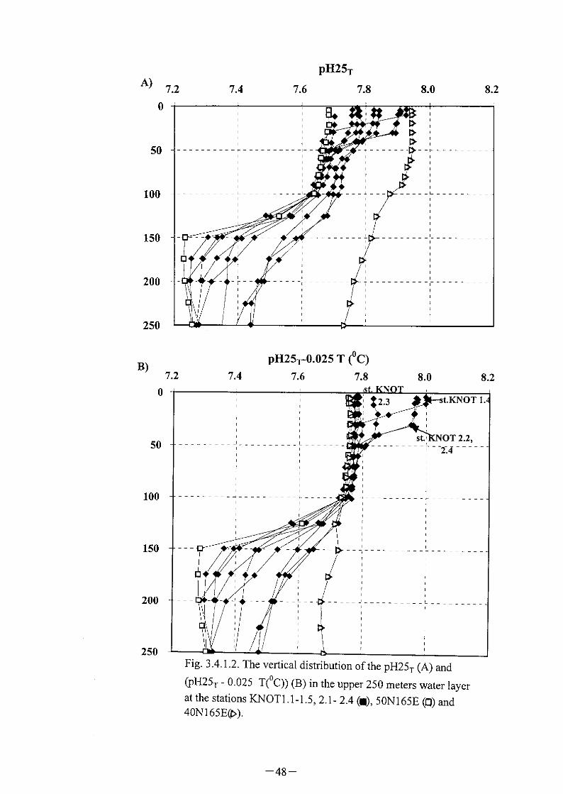
At the Fig. 3.4.1.2.A there are shown vertical profiles of the pH25T in the upper 250 meter water layer
at the stations KNOT1.1- 1.5, KNOT2.1- 2.4, 50N165E and 40N165E.
The pH of the seawater in the upper water layer can be expressed as some initial value pH0 plus
pHexcess (the decrease of the pH due to the increase of the concentration of the CO2 in the atmosphere)
and plus ∆pHbiol. (the change of the pH due to biological activity: inorganic carbon and nutrients
assimilation, organic matter decomposition and calcification)
pH25 =pH250 + pHexcess + ∆pHbiol. (6).
The pH250 is changing with seawater temperature due to the change in pre-form (initial) concentration
of total alkalinity and total alkalinity (Chen et al. 1979).
We estimated that the temperature coefficient of the pH250 in the Northwestern Pacific surface water in
the temperature interval 4- 12 degree C is equal to 0.025 pH unit/degree C (unpublished results of the
expedition MR98K02). Thus the change of the pH due to the biological activity can be determined by
following equation
∆pHbiol.= pH25- pH250- pHexcess = pH25- 0.025•T(0C)- pHexcess- a
, where a is constant.
Fig.3.4.1.2.B shows the distribution of the pH25T-0.025•T (where T is the temperature of the
seawater) in the upper 250 meters water layer at the study stations.
Based on the results of our calculation the increase of the partial pressure of the CO2 in the atmosphere
from the pre-industrial value (about 280 (atm) to the 360 (atm (the averaged measured value of the pCO2
in the atmosphere of the Northwestern Pacific during cruise) should result in the decrease of the pH25 at
0.10- 0.11 pH unit in the upper surface layer. Thus absolute value of the pHexcess is equal to 0.10-
0.11 pH unit in the surface water and it decreasing with depth. The variations in the pHexcess value in
the upper 250 meters could not be considerable, hence, the change of the (pH25- 0.025( T) with depth
(Fig.3.4.1.2. B) shows mainly the change of the pH25 due to the biological activity.
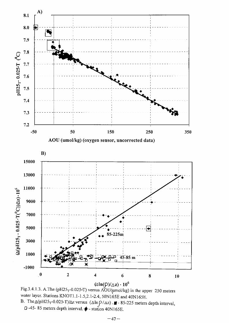
There is linear correlation between Apparent Oxygen Utilization (AOU) values, calculated from
dissolved oxygen, measured by oxygen sensor, and ((pH25- 0.025•T) values (Fig. 3.4.1.3.A).
Using Redfield's model (Redfield et al., 1963) the ratio between the decrease of the pH25 and dissolved
oxygen concentration can be estimated. The decomposition of the organic matter results in the increase of
total inorganic carbon concentration due to the organic carbon oxidation and the decrease of total
alkalinity due to the protonation (Brewer et al., 1979)
∆TCO2org.dec. + ∆TAorg.dec. 0.83•AOU.
In according to our calculations the increase of the total inorganic carbon at 1 (µmol/kg) (when total
alkalinity is constant) and decrease of total alkalinity at 1 (µmol/kg) (when total inorganic carbon is
constant) leads to the decrease of the pH25 at about 0.0025 pH unit. Thus between the AOU and
(pH25biol.activ. the linear relation should exist
∆pH25org.dec. - 0.0028•AOU.
The absolute value of coefficient between change of the (pHT25- 0.025• T) values and AOU in the 250
meter upper water layer at the study stations was lower than 0.0028 probably due to applying uncorrected
dissolved oxygen data, measured by oxygen sensor.
The high values of the (pHT25- 0.025•T) in the surface water layer at the stations KNOT1-4, KNOT2-2,
KNOT2-3 and KNOT2-4 are coincide with low values of the pCO2 of the seawater and are the result of
the considerable assimilation of the inorganic carbon concentration during photosynthesis.
In the 50 - 250 meter layer the pH25 of the seawater is decreasing with depth as the result of the organic
matter decomposition. The location of the maximum vertical gradient in the pH25 values is coincide
with position of the main pycnocline (halocline) (the depth about 125 meter).
The exchange of matter between deep and surface water layers in the study area is limited by
exchange through the main pycnocline. Thus the vertical flux of the dissolved oxygen and dissolved
inorganic carbon is determined by the vertical stability. Fig. Fig.3.4.1.3.B show the linear correlation
between value of the vertical gradient of pH25 and vertical gradient of the density (Fig.3.4.1.3.B) in the
85 - 225 meter water layer.
(4) P r o p o s a l s
T h e m e a s u r e m e n t s o f t h e p H i n t h e s e a w a t e r a r e p l a n n i n g c o n d u c t b y t h e c e l l w i t h o u t t r a n s f e r
C l - i o n r e f e r e n c e e l c t r o d e | test ( s t a n d a r d ) solution | H+ -glass-electrode (D) .
T o t a k e i n t o a c c o u n t t h e c h a n g e w i t h s a l i n i t y t h e c o e f f i c i e n t a c t i v i t y o f t h e c h l o r i d e i o n t h e e q u a t i o n ( 4 ) w
i t h d i f f e r e n t c o e f f i c i e n t c a n b e a p p l i e d .
REFERENCES
Brewer P.G., Wong G.T.F., Bacon M.P and Spencer D.W. An oceanic calcium problem. Earth and
Planetary Science Letters. 1975. V. 26, 81-87 p.
Chen, C.-T. and R. M. Pytkowicz, On the total CO2 - titration alkalinity - oxygen system in the Pacific
Ocean. Nature. 281, 362- 365, 1979.
Dickson, A. G. and C. Goyet (Eds.), Handbook of Methods for the Analysis of the Various Parameters of
the Carbon Dioxide System in Seawater, ORNL/CDIAC-74, 107 pp., 1994.
Redfield A . C . , K e t c h u m B . N . a n d R i c h a r d s F . A . T h e i n f l u e n c e o f t h e o r g a n i s m s o n t h e c o
m p o s i t i o n o f t h e s e a w a t e r . T h e S e a . E d . H i l l . N . - Y . : J . W i l e y a n d S o n s . 1 9 6 3 . V . 2 . P . 2 6 - 7 7
Tishchenko P. A Ch e m i c a l m o d e l o f s e a w a t e r b a s e d o n P i t z e r ' s m e t h o d .
Okeanology.1994. V. 34., P.40-44.
Tishchenko P. Standartization pH measurements of seawater by Pitzerís method. Proceedings of the 2-nd
International Symposium. CO2 in the Ocean.1999. Tsukuba, Japan.
DelValls T.A., Dickson A.G. The pH of buffers based on 2-amino-2-hydroxymethyl-1,3- propanediol
(tris) in the synthetic sea water. 1998. V.45, 1541- 1554.
3.4.2 Total dissolved inorganic carbon
Yuichiro Kumamoto, Akihiko Murata (JAMSTEC)
Kazuhiro Hayashi (MWJ)
Global warming caused by green house gas such as CO2 has become much attention all over the
world. In order to verify carbon cycle in the northwestern North pacific, total dissolved inorganic carbon
(TDIC) was measured with analytical instruments installed on R/V MIRAI.
3.4.2.1 Bottle sampling
Concentration of TDIC in seawater collected at the stations KNOT, 50N, and 40N from surface
to bottom was measured by a coulometer (Carbon Dioxide Coulometer Model 5012, UIC Inc.). A
volume of seawater (35 cm3) was taken into a receptacle and 2 cm3 of 10 percents (v/v) phosphoric acid
was added. The CO2 gas evolved was purged by CO2 free nitrogen gas for 12 minutes at the flow rate of
110 cm3 min.-1 and absorbed into an electrolyte solution. Acids formed by reacting with the absorbed
CO2 in the solution were titrated with hydrogen ions using the coulometer. Calibration of the
coulometer was carried out using sodium carbonate solutions (0-2.5mM). The coefficient of variation
of 3 replicate determinations was approximately less than 0.1 percents for 1 sigma. All the data were
referenced to the Dickson’s CRM and shown in the Appendix.
3.4.2.2 Continuous surface seawater sampling
Concentration of TDIC in surface seawater water collected by a pump from 4 m depth was
continuously measured every 40 minutes by a coulometer (Carbon Dioxide Coulometer Model 5012, UIC
Inc.). A volume of seawater (35 cm3) was taken into a receptacle and 2 cm3 of 10 percents (v/v)
phosphoric acid was added. The CO2 gas evolved was purged by CO2 free nitrogen gas for 12 minutes at
the flow rate of 110 cm3 min.-1 and absorbed into an electrolyte solution. Acids formed by reacting
with the absorbed CO2 in the solution were titrated with hydrogen ions using the coulometer.
Calibration of the coulometer was carried out using sodium carbonate solutions (0-2.5mM). The
coefficient of variation of 3 replicate determinations was approximately less than 0.1 percents for 1 sigma.
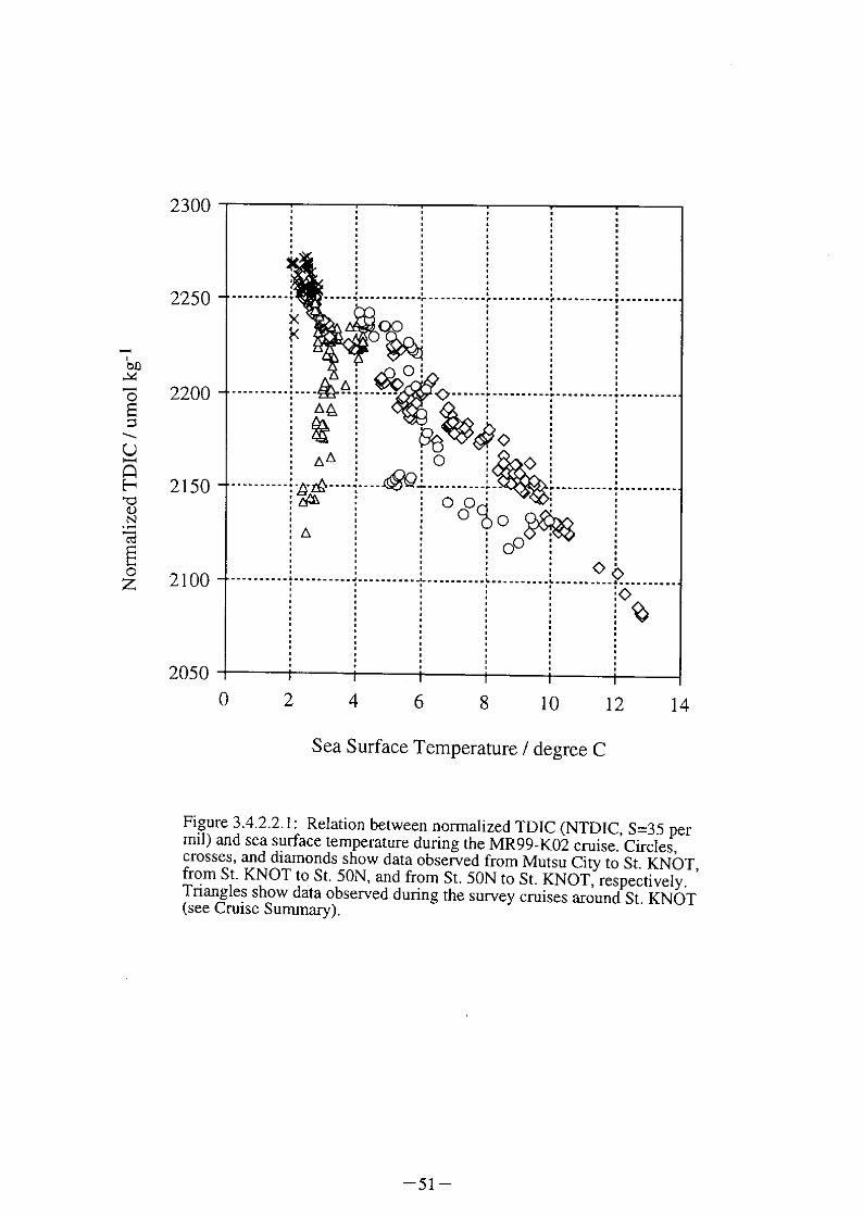
All the data were referenced to the Dickson’s CRM. Figure 1 shows a relation between Normalized
TDIC (NTDIC, S=35 per mil) and sea surface temperature in the surface seawater.
3.4.3 Total Alkalinity
Akihiko Murata (JAMSTEC)
Fuyuki Shibata and Mikio Kitada (MWJ)
Samples were drawn from 12 L drawn from 12 L NiskinTM bottles into 250 ml
polyethylene bottles. Bottles were rinsed twice and filled from the bottom, overflowing
a volume while taking care not to entrain any bubbles. The bottles were then sealed by
a screw cap with an inner cap and stored at room temperature for maximum of 24 hours
prior to analysis.
The total alkalinity titration system consists of a titrator (Radiometer,
TitraLabTM, TIM900) and an autoburette (Radiometer, ABU901). The titration was
made by adding HCl (0.1N) to seawater past the carbonic acid point. Glass
(Radiometer, REF201) and reference (Radiometer REF201) electrodes were used to
measure emf. The repeatability of measured total alkalinity was 0.15 % on average.
All the values reported are set to the Dickson's CRM.
3.4.4 Carbon isotopes
Yuichiro Kumamoto, Makio Honda (JAMSTEC)
Kazuhiro Hayashi (MWJ)
In order to study the role of surface water and intermediate water in carbon cycle in the western
North pacific, seawater for radio and stable carbon isotopes of TDIC was collected by the hydrocast at
the stations KNOT, 50N, and 40N and the underway (continuous) surface seawater sampling. Seawater
was collected in a 250 ml glass bottle. Then a head-space of 2 % of the bottle volume was left by
removing seawater sample with a plastic pipette. Saturated mercuric chloride (HgCl2) of 0.05 cm3 was
added as preservative. Finally, the bottle was sealed using a greased ground glass and a clip was secured.
We collected 240 seawater samples during this cruise. All the samples were stored in a laboratory of
JAMSTEC Mutsu Branch in Mutsu City. In the laboratory, TDIC will be extracted as CO2 and converted
to graphite for measurements of stable and radio carbon isotopes, respectively.
3.4.5 Study of carbon system at the station KNOT
Takeshi Egashira
(Japan Science and Technology Corporation)
(1) Introduction
A new ocean time series station has been established in the western sub arctic Pacific. This is
one of the activities of JGOFS-Japan and JGOFS-NPTT (North Pacific Task Team). This station was
named "KNOT" (Kyodo Northwest Pacific Ocean Time series; Kyodo is Japanese word meaning
collaborative) and located at 44°N, 155°E. The station KNOT is in the southwestern part of western
subarctic gyre and the area is characterized by high biological production in spring/summer and
deepening of surface mixed layer in winter season by surface cooling. The purpose of this study is to
understand the seasonal variation of carbon system in the area around the KNOT.
(2) Methods
(Sampling)
We collected samples for on measurement of total carbon dioxide (TC) and total alkalinity (TA),
carbon dioxide isotope (13CO2), methane (CH4), methane isotope (13CH4), halocarbons and nutrients.
Water samples were collected with CTD rosette systems attached with Niskin bottles of 30L capacity.
Sample waters were drawn from Niskin samplers into individually numbered, clean bottles.
(Sample storage)
TC and TA samples (250ml) were poisoned with 0.05ml of saturated HgCl2 solution and stored
in glass bottles at room temperature. 13CO2
(100ml), CH4(100ml), 13CH4 (30ml or 100ml), and
halocarbons (50ml) samples were poisoned with 0.5ml of saturated HgCl2 solution and stored in glass
bottles at at are refrigerator (5°C). Nutrients samples (100ml) were stored in polypropylene bottles at a
freezer (-20°C).
(3) Future plan
These samples will be analyzed in laboratory on land.
3.4. 6 Dissolved organic carbon
Y. Yamaguchi, Y. Nakaguchi and K. Hiraki
(Department of Chemistry, Faculty of Science and Technology, Kinki University)
(1) Introduction
Dissolved organic matter (DOM) in sea water is one of the largest reservoirs of organic carbon in
the global carbon cycle. It is important to understand the process by which the behavior of oceanic DOM
could affect atmospheric carbon dioxide concentration. On the other hand, DOM plays an important role
in the metal solvilization and scavenging and biogeochemical process in the aquatic environments. So the
investigation of DOM is significant, and it has been done in the world. However the origin of DOM is
poorly understood because the production, decomposition processes and the most of part of chemical
composition has been still unknown. The purpose of this study is to know the seasonal variation of DOM
and to estimate the effect by biological activity. Then, dissolved organic carbon (DOC) was measured by
high temperature catalytic oxidation (HTCO) method at the Stn. KNOT, Stn. HP (High productivity)
and Stn. LP (Low productivity).
(2) Sampling
Sea water samples for determination of DOC were collected from 27 depth at the
Stn. KNOT and 14 depth at the Stn. HP and LP with CTD rosette system equipped with 30 litter Niskin
bottles. Samples were taken from the cast following gas sampling using the in-line filtration system with
pre-combusted Whatman GF/F glass fiber filter. Immediately after collection, the samples were poured
into the pre-combusted 5 ml ampouls in the lab. Then, in order to remove the inorganic carbon, the
samples were acidified by addition of 50 µl 6 N-HCl and bubbling with high purity nitrogen gas. After
these treatments, ampouls in sea water samples were closed up and stored in refrigerator.
(3) Analysis
DOC is assayed by HTCO method using a Shimadzu TOC-5000 analyzer. The frozen samples
were thawed below 5°C, quickly. After thawing of frozen samples, small volumes (100µl) were
sampled and injected in a quartz combustion tube i n a n e l e c t r i c f u r n a c e a t 6 8 0°C a n d f i l l e d w i t h a
p l a t i n u m - a l u m i n u m c a t a l y s t . T h e n , o r g a n i c m a t t e r was o x i d i z e d t o c a r b o n d i o x i d e i n c o m b u s t i o n
t u b e . C o n c e n t r a t i o n o f D O C i s m e a s u r e d a s c a r b o n d i o x i d e b y N o n - d i s p e r s i v e I n f r a - R e d
( N D I R ) a n a l y s e r .
3. 4. 7 W a t e r s a m p l i n g f o r a n a l y s i s o f l o n g - c h a i n u n s a t u r a t e d a l k e n o n e s
N a o m i H a r a d a ( J A M S T E C )
(1) O b j e c t i v e s
L o n g - c h a i n u n s a t u r a t e d a l k e n o n e s c o n t a i n e d i n s e d i m e n t h a v e f o r l o n g , b e e n i n v e s t i g a t e d
a s a r o b u s t p r o x y o f p a s t t h e r m o m e t e r ( e . g . C h a p m a n e t a l . , 1 9 9 6 ) . T h e s e c o m p o u n d s a r e
n o t a b l y b i o s y n t h e s i z e d b y a g r o u p o f h a p t o p h y t e a l g a e , i n p a r t i c u l a r t h e c o c c o l i t h o p h o r i d
E m i l i a n i a h u x l e y i ( E . h u x l e y i ) . T h e a l k e n o n e t h e r m o m e t e r w h i c h h a s b e e n u s e d t o c a l c u l a t e
s e a s u r f a c e t e m p e r a t u r e ( S S T ) i s b a s e d o n t h e u n s a t u r a t i o n r a t i o s o f t h e C 3 7 a l k e n o n e s ,
p r i m a r i l y U K ‘ 3 7
i n d e x. T h e U K ‘ 3 7 i n d e x i s d e f i n e d a s t h e r a t i o o f ( C 3 7 : 2
) / ( C 3 7 : 2
+ C 3 7 : 3 ) , w h e r e C 3 7 : 2 a n d C 3 7 : 3
a r e m e t h y l k e t o n e s w i t h t w o a n d t h r e e d o u b l e b o n d s ,
r e s p e c t i v e l y.
I n o r d e r t o e s t i m a t e t h e p a s t a l k e n o n e t e m p e r a t u r e u s i n g s e d i m e n t c o r e , a c a l i b r a t i o n
e q u a t i o n i s n e c e s s a r y . M o s t p r e c i s e c a l i b r a t i o n i s a n e m p i r i c a l e q u a t i o n i n t r o d u c e d b y a
r e l a t i o n s h i p b e t w e e n U K 3 7 i n d e x a n d S S T i n t h e m o d e r n f i e l d w h e r e t h e s e d i m e n t c o r e w a s
c o l l e c t e d .
I n t h i s s t u d y , t h e r e f o r e , t o o b t a i n a c a l i b r a t i o n f r o m a r e l a t i o n s h i p b e t w e e n t h e U K 3 7
i n d e x and s e a w a t e r t e m p e r a t u r e s at some depths where the alkenone producersnlive in of the
northwestern North Pacific, sea water samples (ca. 5 litters each) were c o l l e c t e d a t t h r e e s t a t i o n s
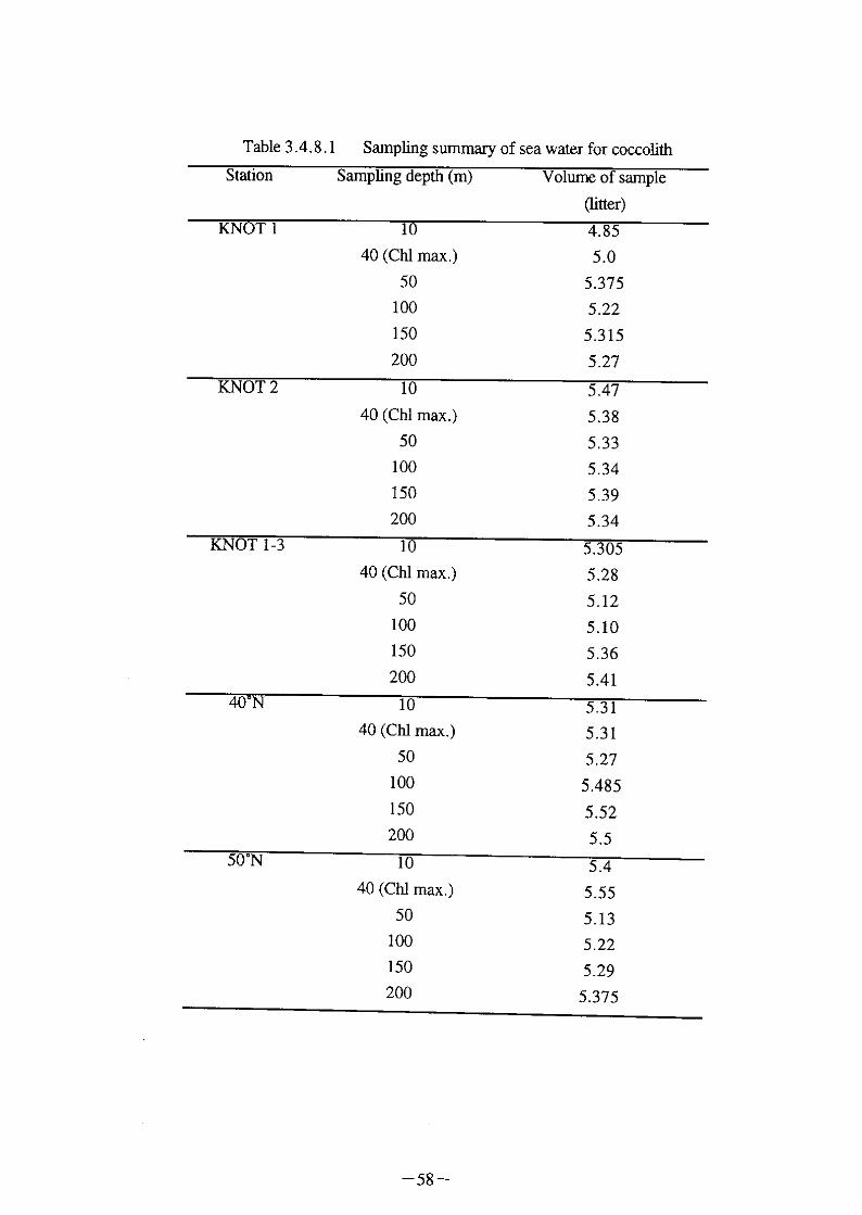
( S t . K N O T , S t . 4 0 ° N a n d S t . 5 0 ° N ) d u r i n g M R 9 9 - K 0 2 c r u i s e . m e t h o d f o r t r a c e m e t a l .
(2) S a m p l i n g p r o c e d u r e o n b o a r d
A t e v e r y s t a t i o n , s e a w a t e r s a m p l e s w e r e c o l l e c t e d i n p l a s t i c b o t t l e s a t s i x w a t e r
d e p t h s : 1 0 m , 5 0 m , 1 0 0 m , 1 5 0 m , 2 0 0 m a n d C h l . m a x i m u m l a y e r ( c a . 4 0 m ) u s i n g a c o m p a c t
C T D r o s e t t e s y s t e m e q u i p p e d o n t h e r i g h t s i d e o f M I R A I ( T a b l e 3. 4. 8. 1) . N i s k i n b o t t l e s w e r e
c l e a n e d b y a method for trace metal before the observation. E v e r y w a t e r s a m p l e i n t h e p l a s t i c
b o t t l e w a s s t o r e d u n d e r - 2 0 ° C i n M I R A I .
(3) A n a l y t i c a l p r o c e d u r e o n s h o r e
E . h u x l e y i a n d G . o c e a n i c a w h i c h a r e a l k e n o n e p r o d u c e r s , a r e c o n c e n t r a t e d o n G F / F
f i l t e r b y a s p i r a t o r y f i l t r a t i o n . T h e s e G F / F f i l t e r s a r e t r e a t e d b y o r g a n i c s o l v e n t e x t r a c t i o n ,
a n d t h e n e v e r y e x t r a c t e d a l k e n o n e i n t h e s o l v e n t i s d e r i v a t i z e d . T h e d e r i v a t i z e d a l k e n o n e
s a m p l e i s i n t r o d u c e d i n t o a g a s c h r o m a t o g r a p h y e q u i p p e d w i t h a F I D d e t e c t o r a n d a c a p i l l a r y
c o l u m n . I n t e g r a t e d a r e a ( i n d i c a t e d a s v o l t a g e ) o f e a c h a l k e n o n e c o m p o u n d i s u s e d t o c a l c u l a t e
t h e U K 3 7 v a l u e .
(4) F u t u r e a n a l y s i s
T h e r e a r e o n l y a f e w i n v e s t i g a t i o n s w h i c h d e t a i l t h e s e a s o n a l v a r i a t i o n o f t h e
r e l a t i o n s h i p b e t w e e n a l k e n o n e f l u x e s a n d a l k e n o n e t e m p e r a t u r e s u s i n g s i n k i n g m a t e r i a l a n d t h e
r e l a t i o n s h i p b e t w e e n t h e a l k e n o n e t e m p e r a t u r e s a n d t h e s p e c i e s c o m p o s i t i o n o f a l k e n o n e
p r o d u c e r s . T h e i n v e s t i g a t i o n o n t h e s e a s o n a l v a r i a t i o n o f a l k e n o n e f l u x e s a n d a l k e n o n e
t e m p e r a t u r e s i n p a r t i c u l a r , h a s n o t b e e n r e p o r t e d f o r t h e n o r t h w e s t e r n N o r t h P a c i f i c . Y e t , i t
i s r e c o g n i z e d t h a t t h e s e a s o n a l v a r i a t i o n o f t h e a l k e n o n e f l u x a n d t e m p e r a t u r e i n t h e u p p e r
l a y e r c o u l d p r o v i d e v a l u a b l e i n f o r m a t i o n f o r u n d e r s t a n d i n g t h e p a s t c h a n g e o f t h e a l k e n o n e
r e c o r d e d i n t h e d e e p s e d i m e n t . I n f u t u r e , t h e r e f o r e , i n o r d e r t o o b t a i n t h e n e w k n o w l e d g e
a b o u t a l k e n o n e s i n t h e m o d e r n n o r t h w e s t e r n N o r t h P a c i f i c , w e w o u l d l i k e t o p r e s e n t a d a t a
s e t o f a l k e n o n e f l u x e s a n d a l k e n o n e t e m p e r a t u r e s w i t h i n t i m e s e r i e s s e d i m e n t t r a p s a m p l e s .
I n a d d i t i o n , w e w o u l d l i k e t o c o m p a r e t h e a l k e n o n e t e m p e r a t u r e r a n g e w i t h t h e d i s t r i b u t i o n
o f a l k e n o n e p r o d u c e r s a n d a c t u a l t e m p e r a t u r e . I n v e s t i g a t i o n s c o n c e r n i n g t h e s e m o d e r n a l k e n o n e
d a t a m i g h t c o n t r i b u t e t o t h e a l k e n o n e t o b e m o r e r o b u s t p r o x y a s a t h e r m o m e t e r .

3.5 Particle organic carbon (POC)
Keiri Imai and Takeshi Egashira
(Core Research for Evolutional Science and Technology)
The stock of particle organic carbon (POC) in euphotic layer is related to the consequences of
biogeochemical processes. Therefore In this cruise it is very important to estimate vertical distribution
of POC. The sample collection and storage is conducted as following.
Water samples were collected with 24L rosette samplers from 13 layers (10, 20, 30, 40, 50, 60, 80, 100,
150, 200, 250, 300 and 500m) at the stations of KNOT1, KNOT2, HP1, HP2, LP1 and LP2. Surface
water samples were collected with clean plastic bucket at above each stations.
Particle matter of subsamples was filtered onto precombusted (450°C, 4h) grass fiber filter (Whatman
GF/F). A filter after fileration was rinsed with particle free salt water and stored frozen (-20 °C) untile
analysis.
3.6 Phytoplankton pigment 3.6.1 Phytoplankton Pigment measurements in the subarctic North Pacific
Kosei Sasaoka
(Faculty of Fisheries, Hokkaido University)
(1) Objectives
Subarctic North Pacific Ocean is one of the highest biological productivity regions in the world.
The quantitative assessment of phytoplankton production in this region is very important to estimate
global primary production. The recent development of satellite ocean color remote sensing and its
application to the observation of the temporal and spatial variability of chlorophyll distribution over
broad area with synoptic scales has provided us with a unique tool to study these features. However, there
is some problems of in-water algorithms in this region. The solar incoming radiation in the subarctic
North Pacific shows large seasonal variability by sky conditions. These radiant environment could effect
the photosynthetic characteristics of phytoplankton in the waters. The bio-optical algorithms in the high
latitude regions were different from the general algorithms (Mitchell, 1992). Then, the new bio-optical
algorithms for the high latitude regions need to be developed as soon as possible. Especially in the winter
season, there is a few bio-optical data sets in this region.
Primary objective of this study is to validate and to develop bio-optical algorithm for new series
ocean color sensors, such as Sea-viewing Wide Field-of-view Sensor (SeaWiFS) and Global Imager
(GLI) in the subarctic North Pacific Ocean. Therefore, we measured in situ bio-optical parameters,
including upwelled spectral radiance, downwelled spectral irradiance, phytoplankton pigment
concentrations (fluorometric method), and particle absorption coefficient. Temporal and spatial valiability
of chlorophyll a were examined using SeaWiFS data which has been received on board.
(2) Water samples for chlorophyll a and absorption coefficient
Water samples for chlorophyll a (Chl-a), pheopigment and absorption coefficient determinations
were collected using Niskin bottles attached to a rosette on the CTD. Chlorophyll samples were collected
at all stations by shallow casts from surface to 200m depth and absorption coefficient samples were
gathered at the stations from surface to 50 m depth, which were carried optical measurements (described
3.14).
Chlorophyll samples were collected in 250 ml bottles and filtered through a Whatman GF/F filter on
board. Filtering Volume was 200 ml. Filtered samples were extracted in 6 ml of N,N-dimethylformamide,
under cold and dark conditions for later analysis. Chl-a and phaeophytin were determined by the
fluorometric method (Parsons et al., 1984) with a Turner Designs Fluorometer (Model:10-AU). Chl-a
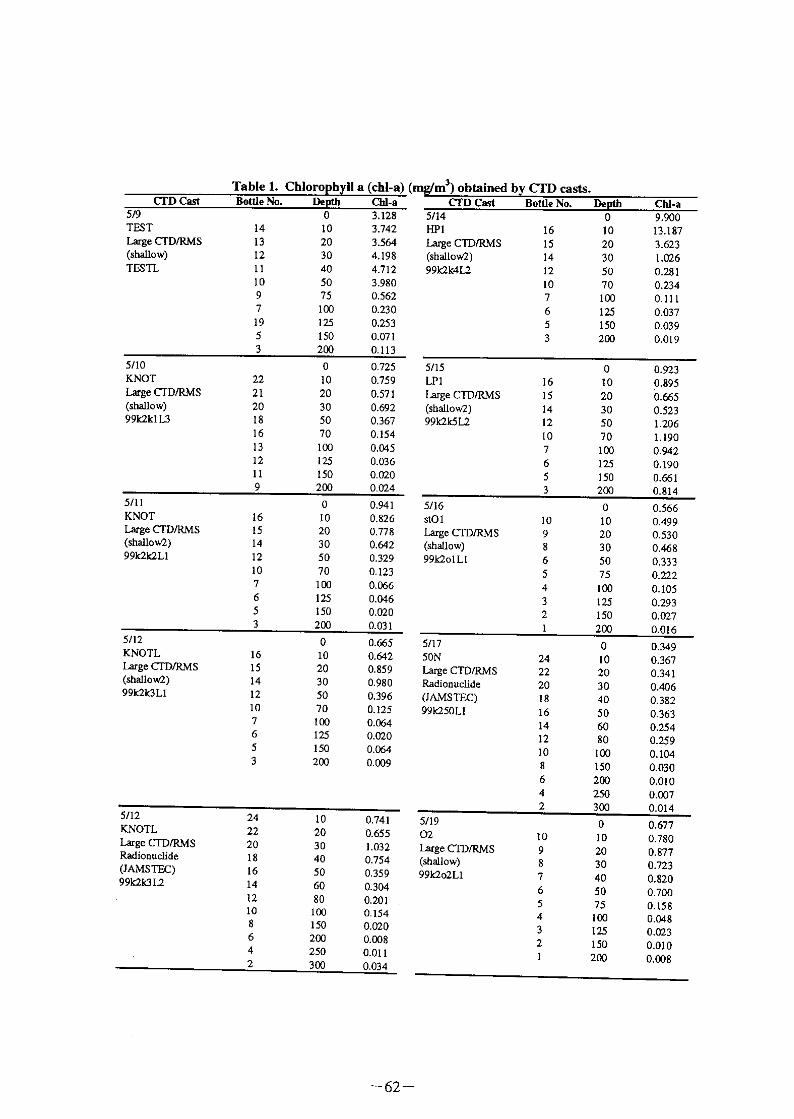
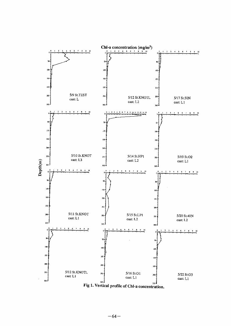
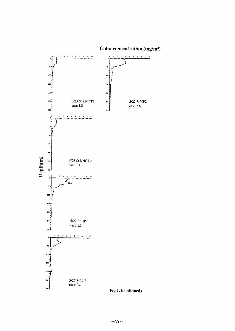
obtained by the CTD casts, summarized in Table. 1, and vertical profiles of chl-a concentration are shown

in Fig. 1. We will compare of these chlorophyll data sets and SeaWiFS data sets in future study.
The absorption coefficients samples were collected in 4000 ml bottles and between 1000 and 3000 ml
filtered on to a 25 mm Watman GF/F glass-fiber filters under low vacuum pressure (<100 mmHg) on
board.
We will measure the absorption coefficients of phytoplankton (aph) and detritus (ad) using the
modified glass fiber technique with methanol treatment (Kishino et al., 1985), and then we will calculate
a chlorophyll normalized specific absorption spectra, a*ph to divide aph by Chl-a concentration. In future
study, we are going to use these chlorophyll a and absorption coefficients for the model parameter to
estimate primary production from satellite ocean color data.


3.6.2 Phytoplankton pigments
Keiri Imai and Takeshi Egashira
(Core Research for Evolutional Science and Technology)
Chorophyll a and pigments separated by HPLC are measured for comparison with
phytoplankton species and number. The seawater subsamples for Phytoplankton piguments collected
from 12 layer(0, 10, 20, 30, 40, 50, 60, 80, 100, 125, 150, 200m) by niskin sampler attached to
CTD-RMS at same stations as primary production experiments. Chorophyll a samples were carried
out size fraction with nuclepore filter(pore size 10, 2um) and grass fiber filter (Whatman GF/F). In Grid
Survey to curry out spring bloom patch study (HP2), surface seawater were collected with seawater pump
of EPCS system. And Chorophyll a samples were made with grass fiber filter (Whatman GF/F).
These Chorophyll a samples will be measured with Turnuer.
3.7 Trace metal - Behavior of iron in the Northwestern North Pacific Ocean.-
Shigeto Nakabayashi
(Japan Marine Science and Technology Center)
(1) Introduction
Fe is one of the major elements in the earth's crust. However, its concentration
in seawater is extremely low. This low concentration is attributed to the fact that
solubility of thermodynamically stable Fe(III) is very low. In other wards, Fe in
seawater readily hydrolyzes to form insoluble colloidal hydrous ferric oxides, settling
down to the bottom. Because of this high reactivity, its residence time in the ocean is
one of the shortest, which is on the order of few hundreds years in deep water and
several weeks in surface water.
Usually an element with a long residence time does not respond to the sudden
change of input or output. However, an element with a short residence time like Fe
changes its concentration in the seawater according to the change of input or output, so
that it is a very good tracer for short term phenomenon.
Fe is supplied from river and atmosphere to the ocean surface. However,
because of its rapid removal from seawater, riverine dissolved Fe is readily removed
within estuary, so that influence of riverine input to the open ocean surface may not be
recognized. Therefore the airborne dust has been proposed as a major source of
dissolved Fe to the open ocean surface. On the other hand, in deep waters other
sources of dissolved Fe have been proposed as the partial release of Fe from
resuspended sediment particles including colloid, and the diffusion from the pore water
in the sediment.
Fe has been also known as an essential micro-nutrient for the phytoplankton
growth in the ocean. Due to its extremely low solubility, however, the concentration
becomes so low that phytoplankton growth is subdued where its supply is limited.
Thus, the fate of Fe in seawater is closely related to the biological activity. It is very
important to know the behavior of Fe in the ocean for the study of the global
biogeochemical cycles of carbon and its related elements.
The Northwestern North Pacific Ocean is characterized by upwelling of deep
water, high nutrients, high primary production and complicated water mass structure
(i.e. intermediate water), among others. And also large aeolian input of terrigeneous
material to the area is expected. Generally, in the North Pacific the dominant source
of the terrigeneous material is Asian dust. Because they can supply Fe over the

surface water, they have significant impact on the phytoplankton growth. In addition,
seasonal and geographical changes of these features are drastic. This complexity has
prevented us from knowing exactly to what extent it plays a role in the global material
cycles, which is a main goal of this project. One of the objectives of this study is to
clarify the role of Fe in the phytoplankton growth in the Northwestern North Pacific.
The other objective is to evaluate the transport and transformation processes of
terrigeneous material and intermediate water in these regions using Fe as a tracer.
(2)Methods
Water samples were collected vertically at 11 stations using acid-cleaned new
type 12 l Niskin-X sampling bottles (General Oceanics) attached to CTD-RMS. As
mentioned above, Fe in the seawater is extremely low, so we have to take special care
before, while and after taking water samples. Sampling bottles with internal closing
mechanism may also be prone to contamination, however this new type sampling bottle
has its stainless steel spring closures mounted externally. This method of mounting
the springs is ideal for applications such as trace metal analysis where the inside of the
sampling bottle must be totally free of contaminants. In addition, inside the sampling
bottles were coated with Teflon to avoid contamination. Teflon stopped cock, Teflon
air vent screw cock and biton o-ring were also used for the bottles. Moreover the steel
hydrowire was sheathed in plastic heat-shrink tubing for 10 m above the rosette as an
effort to minimize contamination from the hydrowire. CTD parameters were
measured on the down and up casts, and water samples taken on the up cast. Surface
seawater samples were collected in acid-cleaned low density polyethylene bottles
directly hanging on a nylon rope. Sampling stations are listed in Table 1.
Sample bottles were of acid-cleaned low density polyethylene and were handled
and stored in polyethylene bags. Water samples for total Fe (100 ml) were kept in a
freezer (-20�C) immediately after sampling.
Samples for dissolved Fe(III) were filtered in- line using a peristaltic pump
system through the acid-washed 25 mm diameter, 0.2 µm Nuclepore polycarbonate
filters held in Teflon filter sandwiches. The filtrates (100 ml) were adjusted to pH 3.2
with formic acid-ammonium format buffer solution and then were kept in a refrigerator
(4�C) until the measurements. This peristaltic pump system comprised a Masterflex
L/S multi-pump head peristaltic pump (Cole-Palmer model PA-41B) with a Masterflex
L/S Standard pump head (Cole-Palmer model 07016-21) containing a short length of
PharMed tubing (Norton size 1.59 mm i.d., 3.18 mm o.d.) connected to a Teflon tubing
(PFA size 1.59 mm i.d., 3.18 mm o.d.) and Teflon filter sandwiches (SAVILEX
2-25-2T).
Samples for colloidal Fe(III) (100 ml) were adjusted to pH 3.2 with same buffer
solution without filtration and were kept in a refrigerator (4�C). Samples for
calibration (only 0 and 10 m, 250 ml) and other dissolved trace metals (250 ml) were
also filtered using same procedure and were kept in a freezer (-20�C). All procedures
were done in a class 100 laminar flow cabinet to avoid contamination. Treatment of
samples are listed in Table 2.
(3)Future plane
Fe(III) will be measured by automated analytical method using a combination of
selective column extraction and luminol-hydrogen peroxide chemiluminescence
detection method. It will be clarify the behavior of iron in the Northwestern North
Pacific during this cruise. Fe has been known as an essential micro-nutrient for the
phytoplankton growth in the ocean. Due to its extremely low solubility, however, the
concentration becomes so low that plankton growth is subdued where its supply is
limited. Thus, the fate of Fe in seawater is closely related to the biological activity.
It is very important to know the behavior of Fe in the ocean for the study of the global
biogeochemical cycles of carbon and its related elements. One of the objectives of
this study is to clarify the role of Fe in the phytoplankton growth in this region during a
spring bloom, especially.
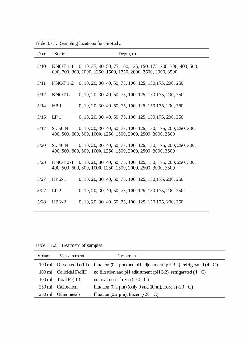
Table 3.7.1. Sampling locations for Fe study.
Date Station Depth, m 5/10 KNOT 1-1 0, 10, 25, 40, 50, 75, 100, 125, 150, 175, 200, 300, 400, 500, 600, 700, 800, 1000, 1250, 1500, 1750, 2000, 2500, 3000, 3500 5/11 KNOT 1-2 0, 10, 20, 30, 40, 50, 75, 100, 125, 150,175, 200, 250 5/12 KNOT L 0, 10, 20, 30, 40, 50, 75, 100, 125, 150,175, 200, 250 5/14 HP 1 0, 10, 20, 30, 40, 50, 75, 100, 125, 150,175, 200, 250 5/15 LP 1 0, 10, 20, 30, 40, 50, 75, 100, 125, 150,175, 200, 250 5/17 St. 50 N 0, 10, 20, 30, 40, 50, 75, 100, 125, 150, 175, 200, 250, 300, 400, 500, 600, 800, 1000, 1250, 1500, 2000, 2500, 3000, 3500 5/20 St. 40 N 0, 10, 20, 30, 40, 50, 75, 100, 125, 150, 175, 200, 250, 300, 400, 500, 600, 800, 1000, 1250, 1500, 2000, 2500, 3000, 3500 5/23 KNOT 2-1 0, 10, 20, 30, 40, 50, 75, 100, 125, 150, 175, 200, 250, 300, 400, 500, 600, 800, 1000, 1250, 1500, 2000, 2500, 3000, 3500 5/27 HP 2-1 0, 10, 20, 30, 40, 50, 75, 100, 125, 150,175, 200, 250 5/27 LP 2 0, 10, 20, 30, 40, 50, 75, 100, 125, 150,175, 200, 250 5/28 HP 2-2 0, 10, 20, 30, 40, 50, 75, 100, 125, 150,175, 200, 250
Table 3.7.2. Treatment of samples.
Volume Measurement Treatment
100 ml Dissolved Fe(III) filtration (0.2 µm) and pH adjustment (pH 3.2), refrigerated (4�C)
100 ml Colloidal Fe(III) no filtration and pH adjustment (pH 3.2), refrigerated (4�C)
100 ml Total Fe(III) no treatment, frozen (-20�C)
250 ml Calibration filtration (0.2 µm) (only 0 and 10 m), frozen (-20�C)
250 ml Other metals filtration (0.2 µm), frozen (-20�C)

3.8 Gas 3.8.1 Halocarbon
Shinya Hashimoto and Tsutomu Mikami
(Tokyo university of fisheries)
(1) Introduction
The measurement of halocarbons in seawater sample was carried out in the
North Pacific Ocean, an area that exhibits relatively high plant
productivity in the water column. The research was carried out during the
cruise conducted on board the research vessel Mirai during May, 1999. The
sampling sites were 12 stations. The maximum depths of sampling stations
were from 5000 m at Stn. 40N and 50N. Water samples were collected from
several depths at each station with a CTD-rosette sampler fitted with 24
Niskin sample bottles of 30 l volume (General Oceanics).
(2) Methods
The water sample was collected in 40 ml brown colored glass bottle (I-CHEM
Certified 200, Nalge Company) for the measurement of halocarbon. After
overflow of more than 100 ml of water, 0.5 ml of HgCl2 was added to inhibit
microbial activity, and the sample bottle was immediately sealed with a
septa (PTFE/silicone) with care to exclude air bubbles, and stored in the
box (in the dark) and kept at 4 C in refrigerator. Samples containing air
bubbles were discarded. The final concentration of HgCl2 in sample bottles
was about 350 mg/l.
(3) Preliminary results
Distribution of halocarbon concentrations in the North Pacific Ocean was
examined to evaluate this oceanic area, with relatively high plant
productivity in the water column, as a natural halocarbon source in this
season. Relatively high concentrations of halocarbons in surface water
were detected in the area of low concentration of pCO2. Both
distributions of halocarbons and correlations among halocarbons showed that
there was some sources of halocarbons in seawater in this area.
3.8.2 Measurement of halogenated volatile organic confounds
Sachiko Nomura, Masahiro Narukawa and Kimitaka Kawamura
(Institute of low temperature science, Hokkaido University)
(1) Introduction
The ocean is the main reservoir of chlorine, bromine, and iodine on the earth. Various types of
macroalgae and phytoplankton are capable of producing halogenated hydrocarbons. Halocarbons formed
in the algal cells are transferred to the seawater across the cell walls.
Volatile halocarbons are emitted from the ocean to the atmosphere, and where they are
photodissociated to result in the release of halogen atoms. Because the halogen atoms are highly
reactive, they have an influence on the oxidation of many organic and inorganic species in the
troposphere. Therefore, measurements of the halocarbons in the ocean and atmosphere should provide
information on atmospheric chemistry.
In order to understand the global distribution of these halocarbons, more observations are needed
in more locations. In this investigation, we measured the natural halocarbons both the seawater and air
samples in the western North Pacific.
(2) Sampling and Methods
Seawater samples (50ml, 100ml) were collected at 7 stations (St. T, St. KNOT, St. O1, St. 50N,
St. O2, St. 40N and St. O3) during a cruise of MR99-K02 in the western North Pacific. The samples
were transported to the lab in Sapporo. Halocarbons will be measured using a purge and trap system with
a gas chromatograph/mass spectrometer (GC/MS). The water samples are purged by nitrogen and
concentrated with the carbon trap. The concentrated gases are transferred to GC/MS.
(3) Future Plan
Seawater sample will be analyzed for halocarbons by purge and trap system with GC/MS. Using
large volume of seawater, we will detect polyhalocarbons, which is organic carbon with many halogen
atoms. Using a chlorophyll-a data, we will discuss in the detail on the production of halocarbons during
the spring bloom.

3.9 Water collection for TFA
Nobuyoshi Yamashita (National Institute for Resources and Environment)
Kurunthachalam Kannan (Michigan State University)
(1) Introduction
The initial concern over TFA was the possible atmospheric conversion of freon replacements
(HFCs). They were expected to increase to 200 ng/L in precipitation by 2010. For some samples which
have already have exceeded that level. Preliminary results show (5-day back trajectories) that air masses
passing over industrial areas contain high concentrations of the HAAs, including TFA. As TFA was in
archived cloud water samples which analyzed, freon replacements are not the sole source of this
compound. It may be guess the major question is how fast is this material accumulating in the
environment and to what final levels?
It is very interesting in obtaining Pacific Ocean samples and compare them to previous results.
Previously we had analyzed samples from profiles collected from the Canada Basin, Eastern Arctic and
the Atlantic Ocean. In general, these samples contained TFA at concentrations greater than 120 ng/L.
Below 900 m in the Canada Basin the water is believed to be greater than 300 years old. This implies
that the TFA is present not as a result of man's latest activities, such derived from freon replacements.
In fresh water systems, adjacent to little or no industrial activity, the concentrations of TFA is less than 10
ng/L. This finding implies that the TFA found in the oceans is naturally occurring or resulting from some
human activity from long ago.
(2) Methods
Sample were taken at pre-determined depths with Go-Flo sampler. Sample volume is about 2
liter.
Blanks: 6L of ultraclean water. Sample bottles were rinsed 1 x with about 50 ml of blank water.
Samples were to be stored at 4°C or equivalent (frozen is better) refrigerator temperature HSSs are
relatively stable at low temps in water.
(3) Sample list
May 10, 1999 Stn. KNOT
duplicate collection
depth (m), 3, Chl-a max, 10, 20, 30, 40, 50, 75, 100, 125, 150, 175
May 22, 1999 Stn. O3
duplicate collection
depth (m), 3, Chl-a max, 10, 20, 30, 40, 50, 75, 100, 125, 150, 200

(4) Future plan
Same kind of water collection are planned in the KH99-3 (Hakuho maru) and other research
cruise with full support in future.

3.10 Radionuclides
3.10.1 234Th by JAMSTEC
Hazime Kawakami (JAMSTEC)
(1) Purpose of the study
Particle-reactive radionuclide (234Th) and their relationship with POC and PON in the
northwestern North Pacific Ocean.
(2) Sampling
Seawater sampling for 234Th : 5 stations (Stn. KNOTL, 50N, 40N, KNOT2, HP2). 12
depths (10m, 20m, 30m, 40m, 50m, 60m, 75m, 100m, 150m, 200m, 250m, 300m) at each
station and 20 liters for each depth.
Seawater samples were filtered with 47mm GF/F filter on board immediately after water
sampling.
(3) Chemical analyses
Separations of U and Th were used by anion exchange method on board; Dissolved and
particulate samples of Stn. KNOTL, 50N, 40N and KNOT2. The rest of samples were
separated from U in land-based laboratory.
Separated samples of Th were absorbed on 25mm stainless steel disks electrically, and
were measured by β-ray counter.
(4) Preliminary result
The distributions of dissolved and particulate 234Th will be determined as soon as possible
after this cruise. This work will help further understanding of particle dynamics in the water
column.
3.10. 2 Time-series observation of 234Th, 210Po and 210Pb at KNOT station Koh Harada (National Institute for Resources and Environment)
Yoko Shibamoto (National Institute for Resources and Environment)
Hisashi Narita (Graduate School of Hokkaido University)
Masashi Kusakabe (Japan Marine Science and Technology Center)
(1) Introduction
Since export flux from surface layer to deeper layer is strongly related
with biological production in the surface layer, it is predicted to have a
large seasonal variation. To understand seasonal change of export flux from
the surface layer, the time-series observations of particulate flux by
drifting sediment traps and short lived natural radio nuclides have been
conducted from June 1998. The flux observed by the drifting sediment traps
should be corrected because of non-quantitative collecting efficiency due to
shape of the trap and complicated hydrodynamics in the surface water. The
short lived radio nuclides are good tracers for particulate materials.
Therefore the vertical profiles of the nuclides are planned to use for
correction of the export flux by the drifting traps as well as independent
estimation of the flux from the nuclides profiles.
In this cruise, a water mass with low pCO2
and high chlorophyll was
discovered. To clarify the deference between the water mass and one with
almost same water temperature but high pCO2 and low chlorophyll, samples
from Stn. HPs and LPs were also analyzed.
(2) Methods
About 20-l each of seawater samples were collected at 6 stations from
several layers as follows:
Stn. KNOT-1 0, 10, 20, 30, 40, 50, 60, 80, 100, 125, 150, 200, 300 m
Stn. HP1 0, 10, 20, 30, 40, 50, 60, 80, 100, 125, 150, 200, 300, 500 m
Stn. LP1 0, 10, 20, 30, 40, 50, 60, 80, 100, 125, 150, 200, 300, 500 m
Stn. KNOT-2 0, 10, 20, 30, 40, 50, 60, 80, 100, 125, 150, 200, 300, 500 m
Stn. HP1 0, 10, 20, 30, 40, 50, 60, 80, 100, 125, 150, 200, 300 m
Stn. HP2 0, 10, 20, 30, 40, 50, 60, 80, 100, 125, 150, 200, 300 m

Immediately after the sampling, the seawater samples were filtered through
GF/F filters, acidified and spiked. After standing for 3 to 6 hours, the
samples were neutralized by adding ammonia water and hydroxide precipitates
were formed. The precipitates were collected on cartridge filters. After
some purification and separation treatments using ion exchange and
extraction techniques, Po was plated onto a silver disc, Th was collected in
scintillation solution and Pb fraction was kept in a plastic bottle.
Radio-activities in each fraction are going to be counted in a land
laboratory in NIRE.

3.11 Primary production
Keiri Imai and Takeshi Egashira
(Core Research for Evolutional Science and Technology)
In western region of North Pacific Ocean time series survey was started since June 1998. In
this region it is very important to estimate primary production by phytoplankton in spring. Therefore the
mission of this cruise is to measure primary production of spring bloom by phytoplankton.
In this cruise, using 13C as a tracer for inorganic 13C uptake by phytoplankton photosynthesis,
incubation experiments carried out in two types procedures(in-site and –vivo). Water samples were
collected with lever action niskin bottles attached Kevler wire from the 6 layers corresponding to 100, 34,
17, 8.5, 4, 0.9% of surface irradiance and drained into 250ml polycarbonate bottles. After addition of
13C-NaHCO3 those bottles were incubated for 24h. And particle matter was filtered onto precombusted
(450°C, 4h) grass fiber filter (Whatman GF/F) after incubation. Primary production will be calculated
with concentration and 13C atom % of particle organic carbon (POC) determined by tracer. Incubation
data and station and sampling depth are as follows.
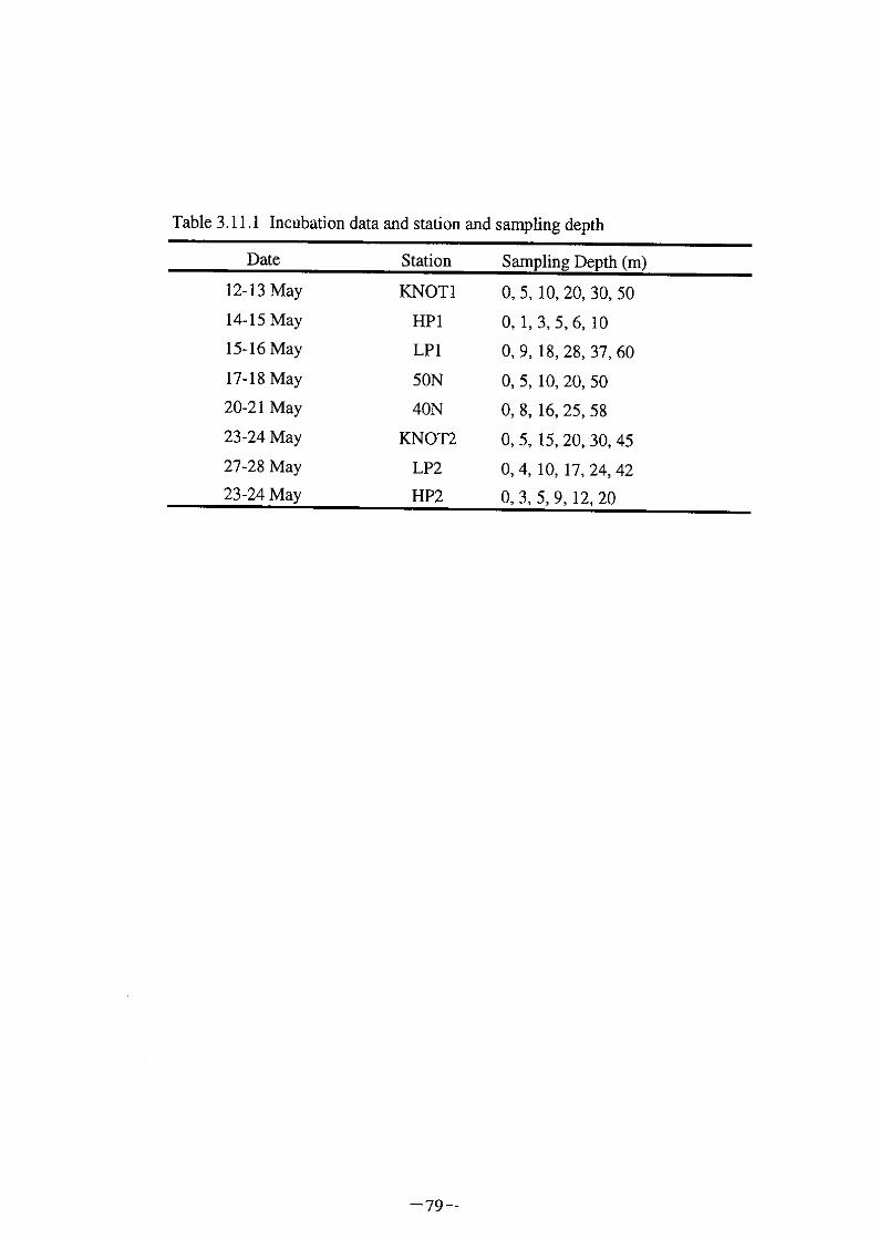
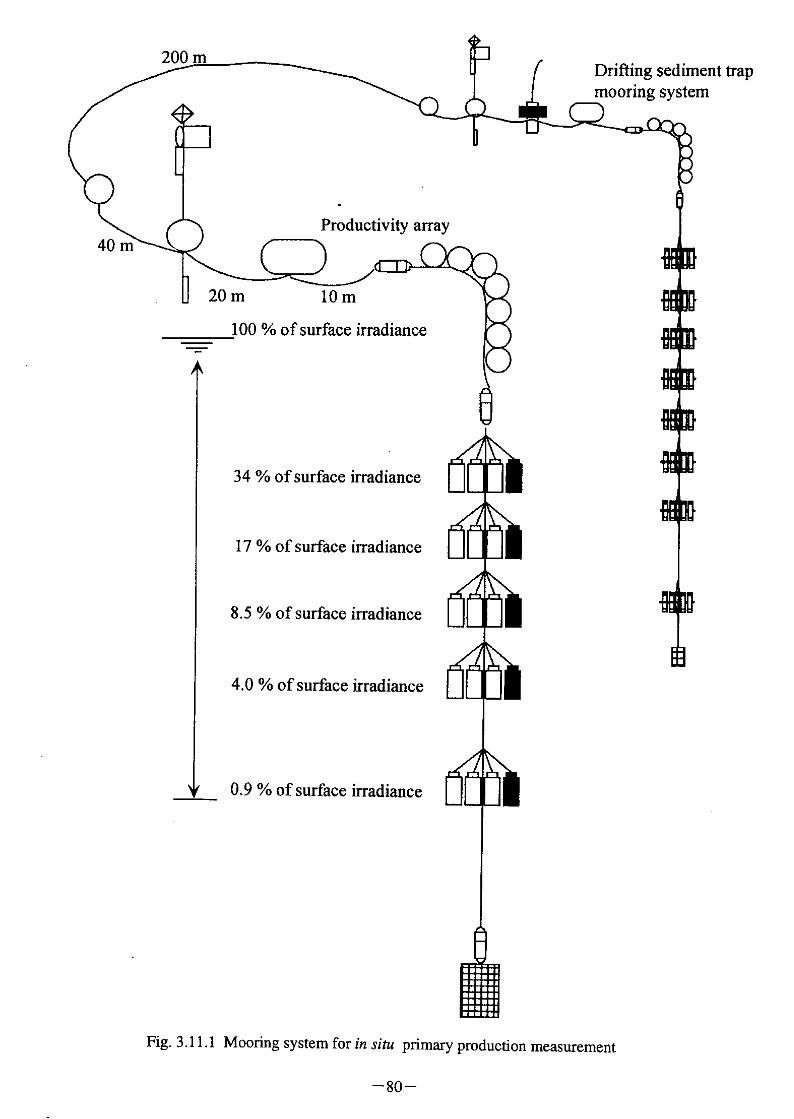

3.12 Drifting sediment trap experiment
Makio Honda (Japan Marine Science and Technology Center)
Hisashi Narita (Hokkaido University)
Keiri Imai (National Institute of Environmental Science)
Koh Harada (National Institute of Resource and Environment)
Sediment trap working group
(1) Introduction
As one of tactics to verify the role of oceanic biological pump in the control of global
environment, time-series sediment trap experiments have been carried out all over the world ocean.
However, time-series sediment traps have been usually deployed in the deep sea (> 1000 m) because of
complication of hydrodynamics, swimmer, and vandalism in the shallower water. Therefore these
sediment traps have not given us enough information about the mechanism of biological pump in the
layer between photic zone and deep sea. In addition, collecting efficiency of moored sediment traps
are significantly affected by hydrodynamics. In order to solve these problem, drifting sediment trap
experiments have been also conducted to collect settling particles in the shallower depth although
experimental period is limited.
For the better understanding of biological pump in spring in the Northwestern North Pacific,
we conducted short-termed drifting sediment trap experiment four times at and around stn. KNOT in
this cruise.
(2) Methods
1) Instrumentation
Sediment trap array consisted of eight individual transparent policarbonate cylinders with
baffle (collection area, ca. 0.0038 m2: aspect ratio, 620 mm length / 75 mm width = 8.27), which were
modified from Knauer et al. (1979) and were deployed from ca. 20 m to 400 m. In order to compare
the result and conduct multi purpose study, two mooring systems were used. Figures 3.11.1 (a) and
(b) show mooring systems by CREST group and JAMSTEC, respectively. Before deployment, each
piece of sediment trap was filled with filtered surface sea water, which salinity was adjusted to ca. 39
PSU by addition of NaCl. Thermometer and depth sensor were attached on CREST sediment trap array.
These sediment traps were lowered from surface floating package including surface floating buoy,
GPS buoy, radar reflector, and flash light.
2) Experiments
Experiments were conducted four times in this cruise (Table 3.11.1). Two mooring systems
were deployed and drifted twice at stn. KNOT at the beginning and the late of this cruise. Judging
from sea water pCO2, DO, and fluorescence observed with underway monitoring system, the spring
bloom has not occurred yet during both period. Other two experiments were conducted in the area
where the spring bloom took place around stn. KNOT (stn. HP1, 2 and LP1). During these
experiments, one mooring system was deployed in this high productivity area and another one was
deployed in the outside of this area where the spring bloom could not be seen.
3) Drifting track
These mooring system drifted during ca. 23 ~ 73 hours at and around stn. KNOT (Table
3.11.1). During the experiment, the position of mooring system was monitored on board by GPS
tracking system. Fig. 3.11.2 (a), (b), (c), and (d) show tracks of two drifting sediment trap mooring
systems during four experiments. As can be seen in figures, two sediment trap mooring systems drifted
drawing spiral pattern and changed these directions simaltaneously, which is indicative of that these
drifting patterns were controled by the small eddy.
4) Variability in depth and water temperature during experiments
Several depth sensors and thermometers were installed on mooring system.
Fig. 3.11.3 (a), (b), (c), (d) show the variability in depths of depth sensors, which installed at
10 m and 190 m on CREST mooring system for each experiments. Depth of 10 m depth sensor
increased from 12 m to 14 m at the beginning of experiment (I), which was attributed to the extension
of mooring rope (Fig. 3.11.3 (a)). After this period, depth of depth sensor was stable with small
amplitude of 0.3 m ~ 1.0 m, which might synchronized with surface waves. Depth of 190 m depth
sensor increased slightly during the experiment. Internal current might raise the mooring system.
During experiment (III), depths of 10 m and 190 m depth sensors decreased around 2:00 of 24 May.
It was caused by the installation of the primary production mooring system at the top of drifting
sediment trap mooring system.
Fig. 3.11.4 (a), (b), (c), and (d) show the change in temperature of each depth during
experiments.
Fig. 3.11.4 (a) show that SST during experiment (I) was approximately 7.5 °C, which was
warmer than the typical water of sub-Arctic water overlying stn. KNOT in spring. Temperature at 40
m increased around 12:00 of 11 May and 3:00 of 12 May. During this period, the surface mixed layer
became thick. It is notable that temperature at 180 m temporally became higher than that at 120 m.
During experiment (II), temperature at 20 m and 40 m decreased significantly between 21:00
on 14 May and 3:00 of 15 May. This time was coincident with the turning point of track of mooring
system (Fig. 3.11.2 (b)). Temperature at 40 m was lower than that at 60 m (Fig. 3.11.4 (b)). These
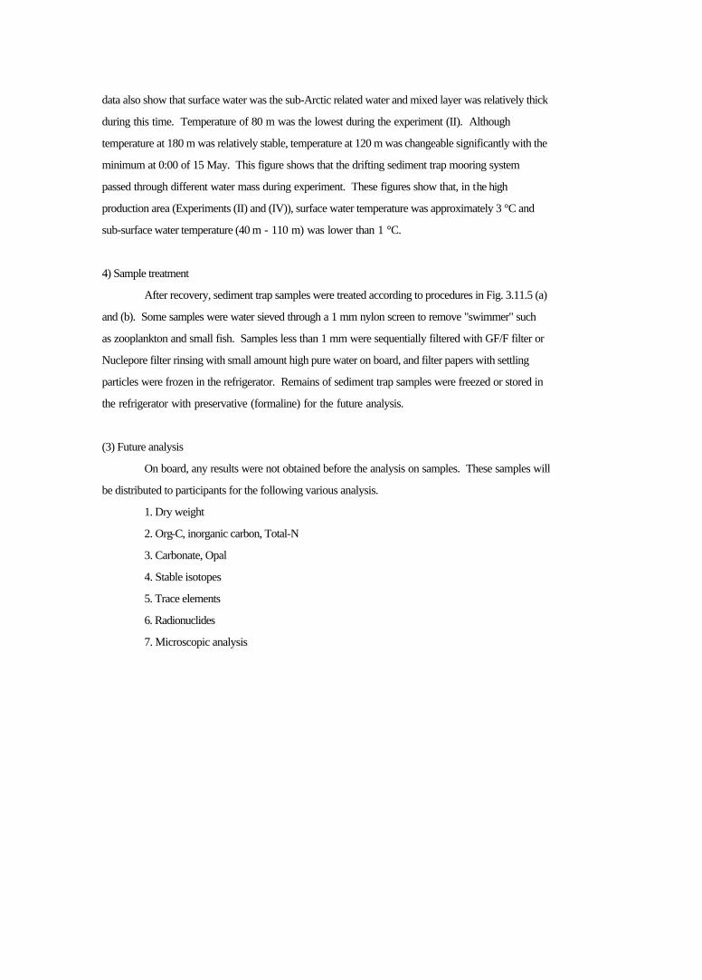
data also show that surface water was the sub-Arctic related water and mixed layer was relatively thick
during this time. Temperature of 80 m was the lowest during the experiment (II). Although
temperature at 180 m was relatively stable, temperature at 120 m was changeable significantly with the
minimum at 0:00 of 15 May. This figure shows that the drifting sediment trap mooring system
passed through different water mass during experiment. These figures show that, in the high
production area (Experiments (II) and (IV)), surface water temperature was approximately 3 °C and
sub-surface water temperature (40 m - 110 m) was lower than 1 °C.
4) Sample treatment
After recovery, sediment trap samples were treated according to procedures in Fig. 3.11.5 (a)
and (b). Some samples were water sieved through a 1 mm nylon screen to remove "swimmer" such
as zooplankton and small fish. Samples less than 1 mm were sequentially filtered with GF/F filter or
Nuclepore filter rinsing with small amount high pure water on board, and filter papers with settling
particles were frozen in the refrigerator. Remains of sediment trap samples were freezed or stored in
the refrigerator with preservative (formaline) for the future analysis.
(3) Future analysis
On board, any results were not obtained before the analysis on samples. These samples will
be distributed to participants for the following various analysis.
1. Dry weight
2. Org-C, inorganic carbon, Total-N
3. Carbonate, Opal
4. Stable isotopes
5. Trace elements
6. Radionuclides
7. Microscopic analysis
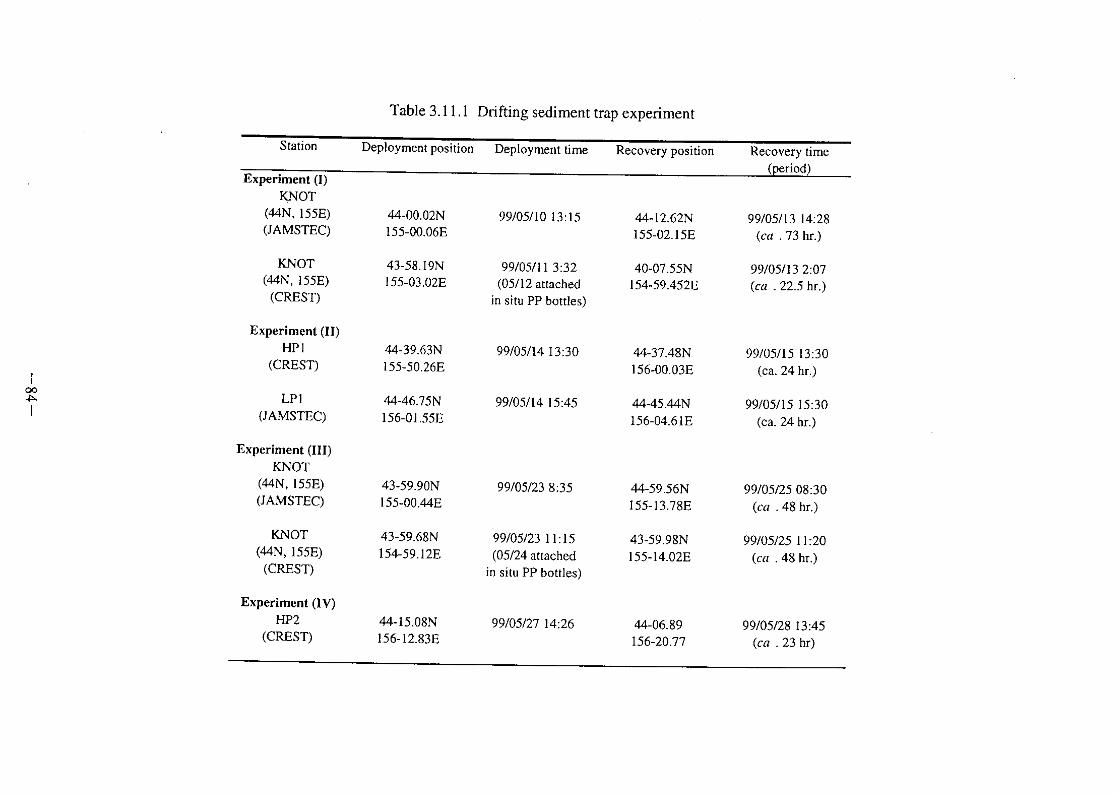
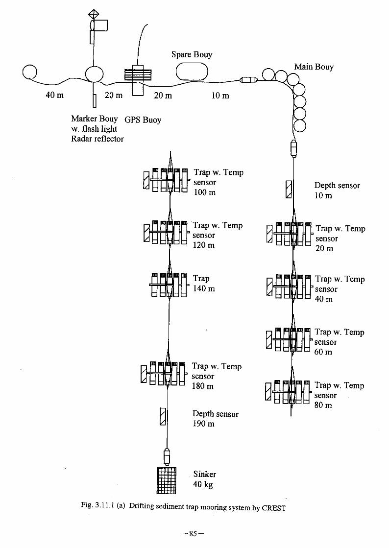


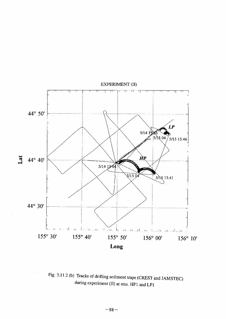

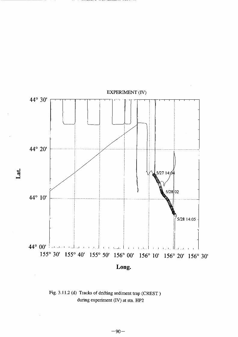
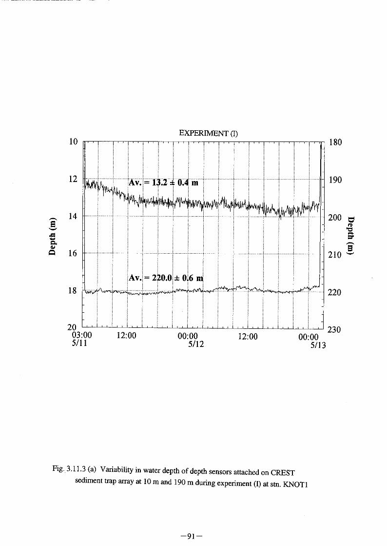
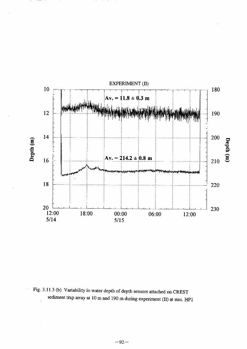
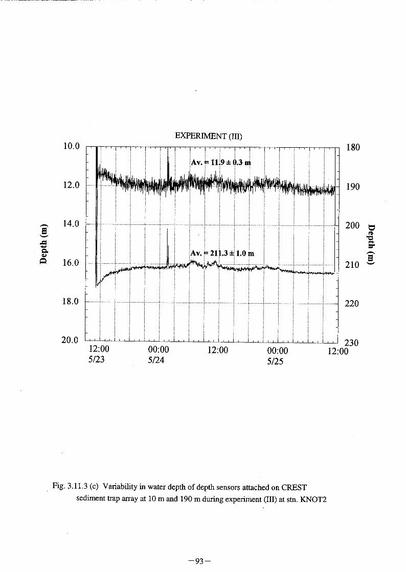
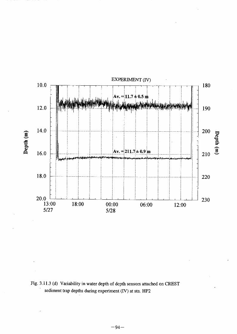


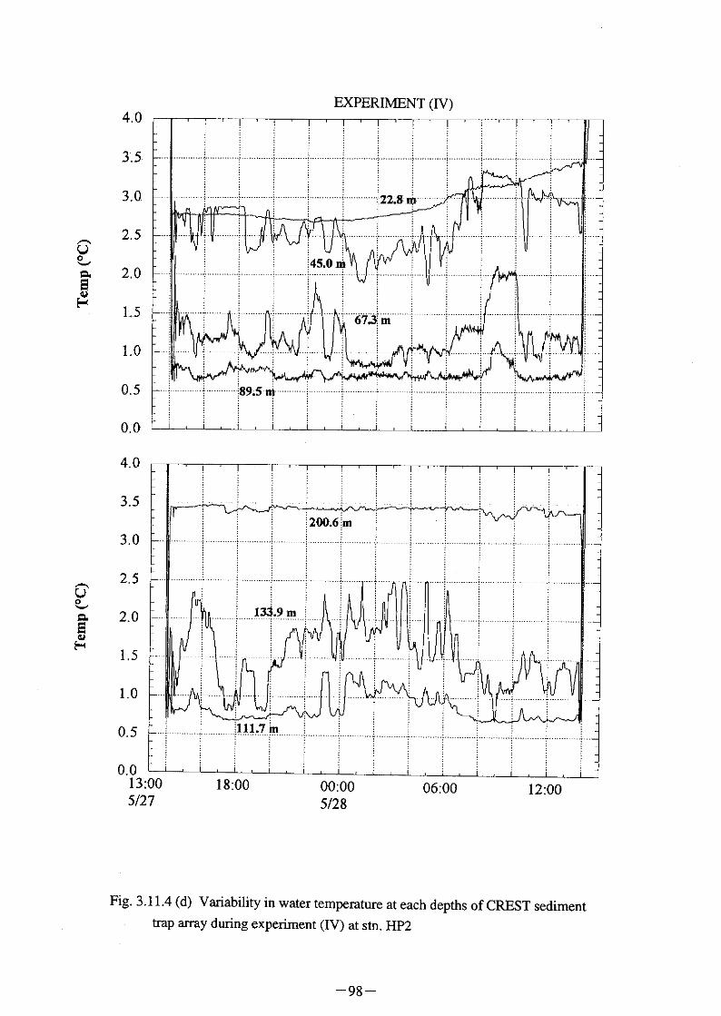

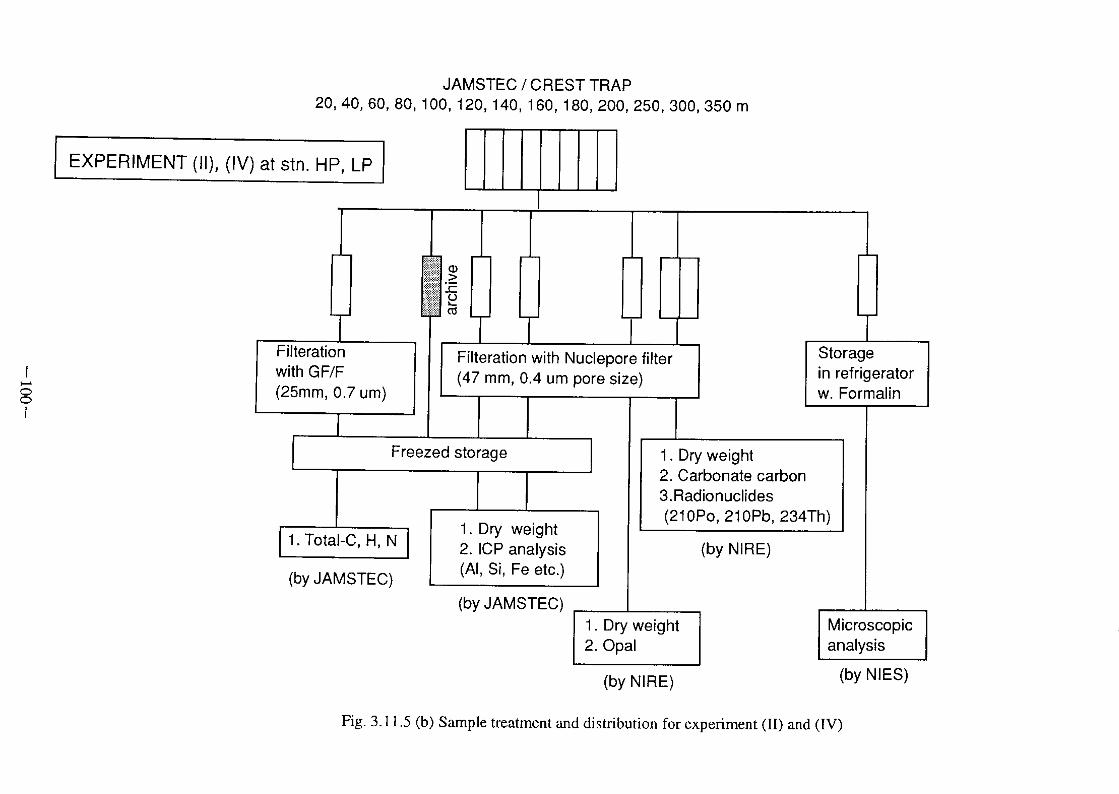
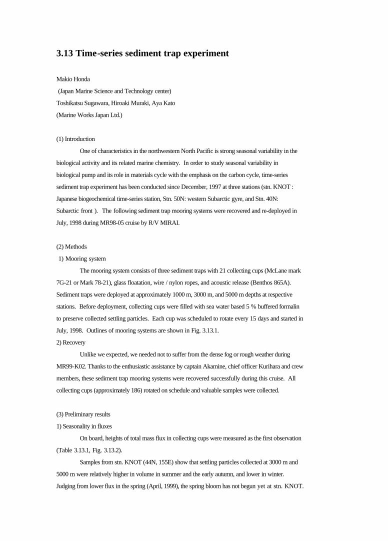
3.13 Time-series sediment trap experiment
Makio Honda
(Japan Marine Science and Technology center)
Toshikatsu Sugawara, Hiroaki Muraki, Aya Kato
(Marine Works Japan Ltd.)
(1) Introduction
One of characteristics in the northwestern North Pacific is strong seasonal variability in the
biological activity and its related marine chemistry. In order to study seasonal variability in
biological pump and its role in materials cycle with the emphasis on the carbon cycle, time-series
sediment trap experiment has been conducted since December, 1997 at three stations (stn. KNOT :
Japanese biogeochemical time-series station, Stn. 50N: western Subarctic gyre, and Stn. 40N:
Subarctic front ). The following sediment trap mooring systems were recovered and re-deployed in
July, 1998 during MR98-05 cruise by R/V MIRAI.
(2) Methods
1) Mooring system
The mooring system consists of three sediment traps with 21 collecting cups (McLane mark
7G-21 or Mark 78-21), glass floatation, wire / nylon ropes, and acoustic release (Benthos 865A).
Sediment traps were deployed at approximately 1000 m, 3000 m, and 5000 m depths at respective
stations. Before deployment, collecting cups were filled with sea water based 5 % buffered formalin
to preserve collected settling particles. Each cup was scheduled to rotate every 15 days and started in
July, 1998. Outlines of mooring systems are shown in Fig. 3.13.1.
2) Recovery
Unlike we expected, we needed not to suffer from the dense fog or rough weather during
MR99-K02. Thanks to the enthusiastic assistance by captain Akamine, chief officer Kurihara and crew
members, these sediment trap mooring systems were recovered successfully during this cruise. All
collecting cups (approximately 186) rotated on schedule and valuable samples were collected.
(3) Preliminary results
1) Seasonality in fluxes
On board, heights of total mass flux in collecting cups were measured as the first observation
(Table 3.13.1, Fig. 3.13.2).
Samples from stn. KNOT (44N, 155E) show that settling particles collected at 3000 m and
5000 m were relatively higher in volume in summer and the early autumn, and lower in winter.
Judging from lower flux in the spring (April, 1999), the spring bloom has not begun yet at stn. KNOT.
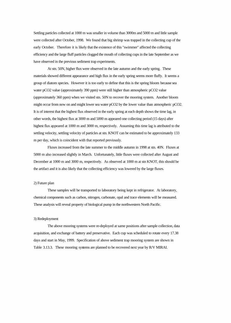
Settling particles collected at 1000 m was smaller in volume than 3000m and 5000 m and little sample
were collected after October, 1998. We found that big shrimp was trapped in the collecting cup of the
early October. Therefore it is likely that the existence of this "swimmer" affected the collecting
efficiency and the large fluff particles clogged the mouth of collecting cups in the late September as we
have observed in the previous sediment trap experiments.
At stn. 50N, higher flux were observed in the late autumn and the early spring. These
materials showed different appearance and high flux in the early spring seems more fluffy. It seems a
group of diatom species. However it is too early to define that this is the spring bloom because sea
water pCO2 value (approximately 390 ppm) were still higher than atmospheric pCO2 value
(approximately 360 ppm) when we visited stn. 50N to recover the mooring system. Another bloom
might occur from now on and might lower sea water pCO2 by the lower value than atmospheric pCO2.
It is of interest that the highest flux observed in the early spring at each depth shows the time lag, in
other words, the highest flux at 3000 m and 5000 m appeared one collecting period (15 days) after
highest flux appeared at 1000 m and 3000 m, respectively. Assuming this time lag is attributed to the
settling velocity, settling velocity of particles at stn. KNOT can be estimated to be approximately 133
m per day, which is coincident with that reported previously.
Fluxes increased from the late summer to the middle autumn in 1998 at stn. 40N. Fluxes at
5000 m also increased slightly in March. Unfortunately, little fluxes were collected after August and
December at 1000 m and 3000 m, respectively. As observed at 1000 m at stn KNOT, this should be
the artifact and it is also likely that the collecting efficiency was lowered by the large fluxes.
2) Future plan
These samples will be transported to laboratory being kept in refrigerator. At laboratory,
chemical components such as carbon, nitrogen, carbonate, opal and trace elements will be measured.
These analysis will reveal property of biological pump in the northwestern North Pacific.
3) Redeployment
The above mooring systems were re-deployed at same positions after sample collection, data
acquisition, and exchange of battery and preservative. Each cup was scheduled to rotate every 17.38
days and start in May, 1999. Specification of above sediment trap mooring system are shown in
Table 3.13.3. These mooring systems are planned to be recovered next year by R/V MIRAI.
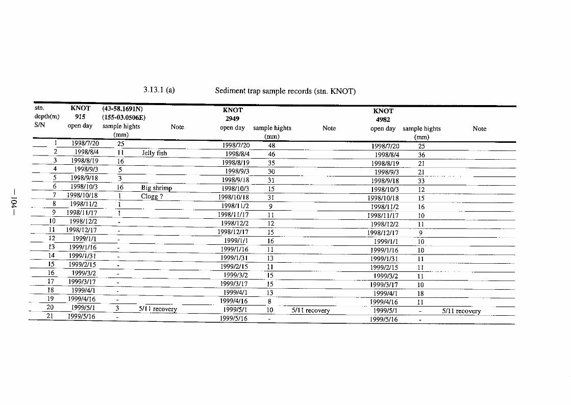
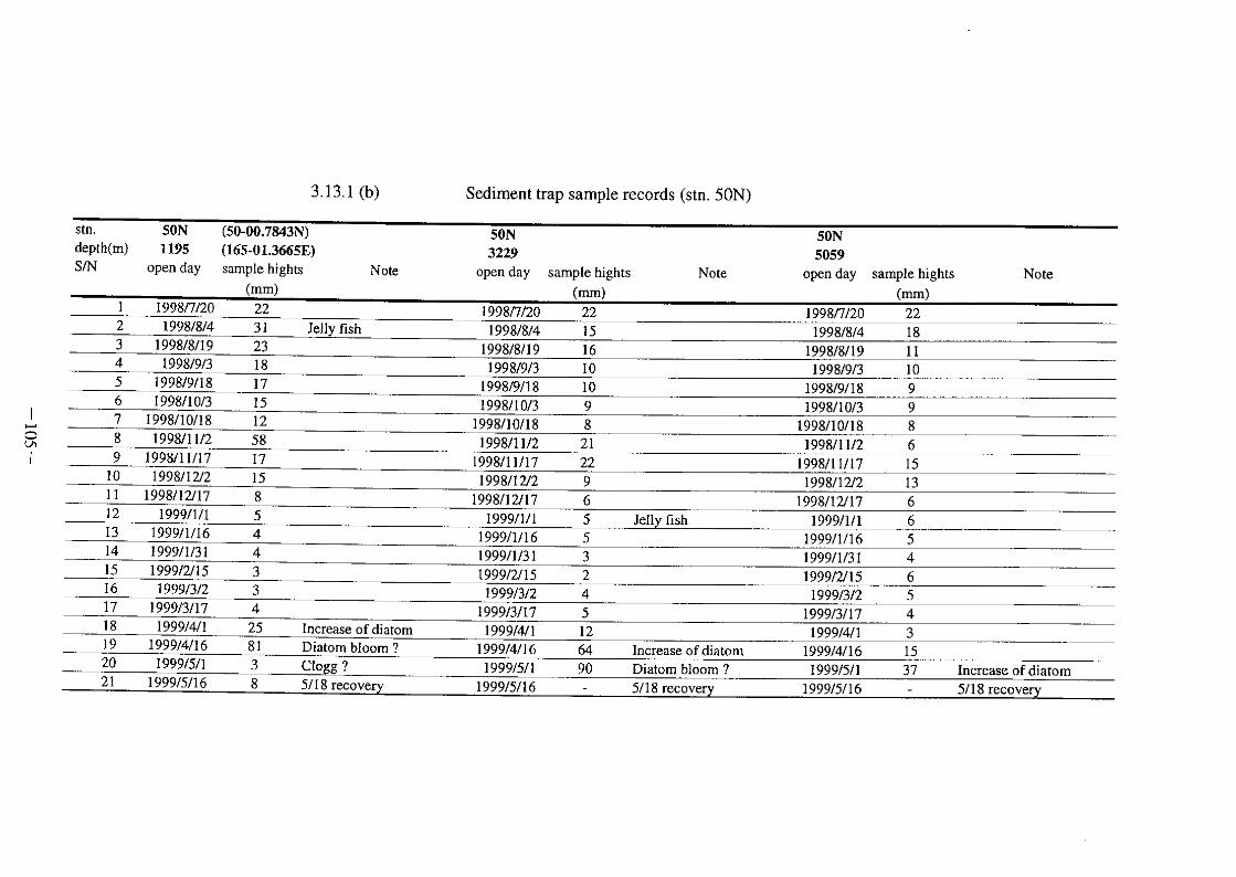


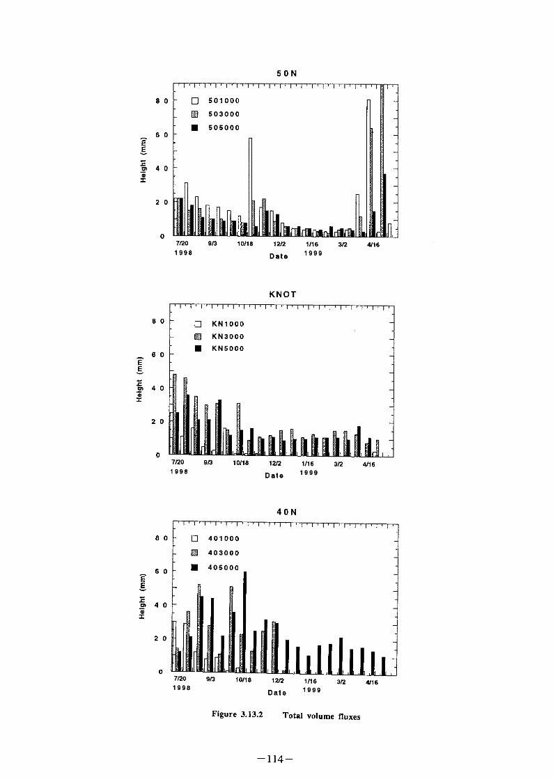
3.14 Bio-optical measurements in the subarctic North Pacific Ocean for ocean color remote sensing
Kosei Sasaoka
(Faculty of Fisheries, Hokkaido University)
The underwater spectral downward irradiance and upward radiance were measured using the
underwater unit, MER-2040 (Biospherical Instrument Inc.). The measurements were carried out from the
sea surface down to depth 100m depending on the water turbidity. The incident solar spectral irradiance
was measured using the deck unit, MER-2041 (Biospherical Instrument Inc.). The measurements were
carried out two times a day near the satellite overpassing time (about 10:00 A.M. and 13:00 P.M.) at Stns.
Knot, O1, 50N, 40N, KNOT2 and HP2. At other stations (St.TEST, HP1, LP1, O2, O3, LP2 and special
stations (19 May, between St.O2 and St.40N and 22 May, between St.O3 and St.KNOT2 )) were made
once a day near the satellite overpassing time (about 10:00 A.M. or 13:00 P.M.). The list of
MER-2040/2041 measurement in this cruise summarized Table 1. The spectral channels of MER-2040 /
2041 covered the wavelength of 412, 443, 465, 490, 510, 520, 555, 565, 625, 665, 670, 683 nm and PAR
(710 nm for upward radiance). These channels were selected for compatible satellite ocean color sensor,
Sea-viewing Wide Field-of-view Sensor(SeaWiFS) and Global Imager(GLI).
Upward and downward PAR (Photosynthetically available radiation) was determined optical
depth for the in-situ primary production measurement (CREST group).
In future study, we will calculate normalized water leaving radiance (Lwn) using these
bio-optical parameters and examine the relationship between in situ measured chl-a values and estimated
chl-a values using the several bio-optical algorithm developed by NASA, NASDA and other researchers.
We will develop the new bio-optical algorithms for the high latitude regions and make high accuracy
chl-a images in this region in future study.
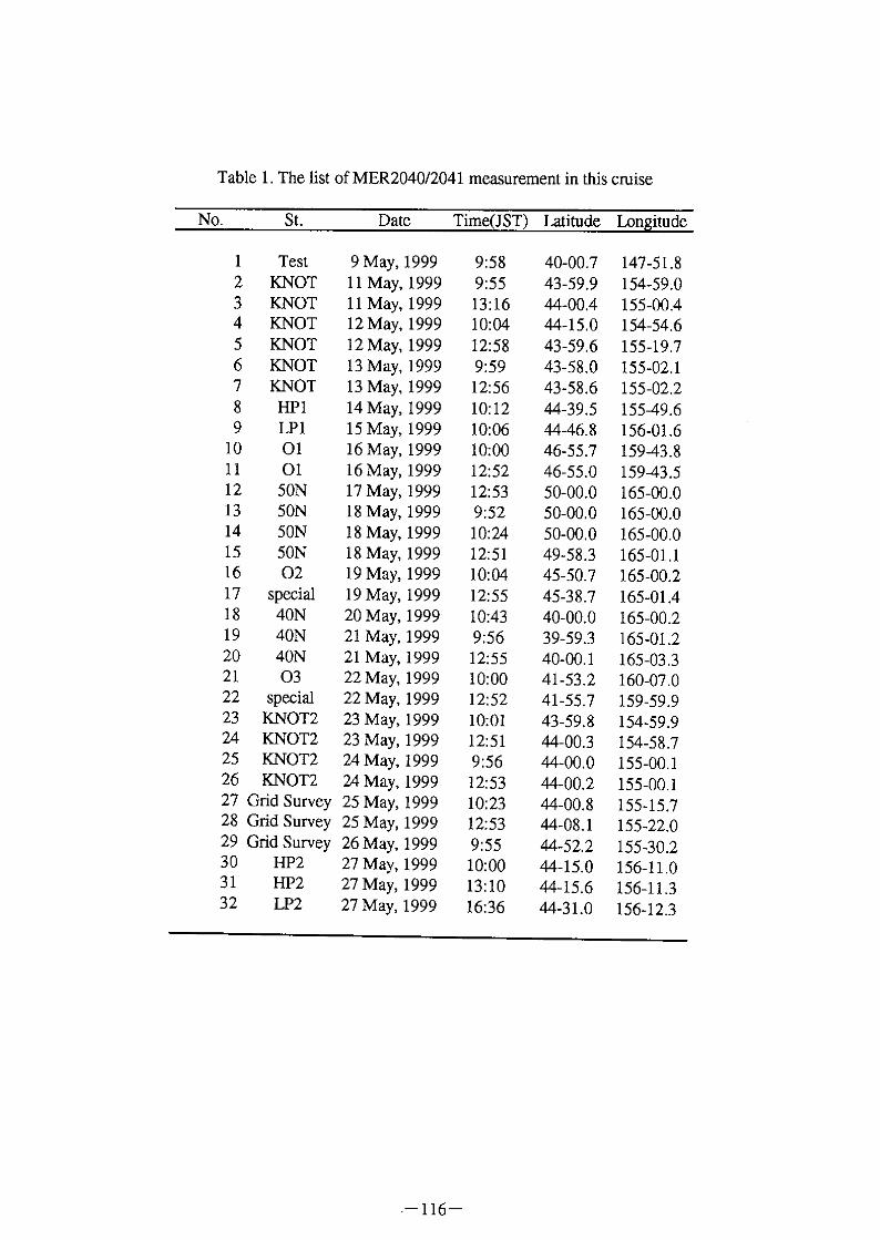
3.15 Plankton
Yuichiro Yamada
(Biological Oceanography Laboratory, Faculty of Fisheries, Hokkaido University)
Keiri Imai
(Core Research for Evolutional Science and Technology)
(1) Net zooplankton
This samplings aims to reveal the biomass, horizontal and vertical distribution, and species
composition of net zooplankton in northwestern subarctic Pacific. Net zooplankton were collected using
three types nets. Palumbo-Chun-Petersen (PCP) type closing net (45cm mouth diameter, 0.06mm mesh)
designed by Kawamura (1989) were made at stn. KNOT 1, 50N and KNOT 2. Sampling depth strata
were 0-50, 50-250, 250-500, 500-1000 and 100-1800m at stn. KNOT 1, 0-100, 100-250, 250-500,
500-1000 and 1000-1500m at stn. 50N, and 0-50, 50-250, 250-500, 500-1000 and 1000-1500m at stn.
KNOT 2. Twin-type (0.33mm mesh) or single type (0.2mm mesh) NORPAC nets (45cm mouth
diameter, Motoda 1957) were towed vertically. Volumes of water filtered through the net were
estimated from readings of a Rigosha flowmeter mounted in the mouth of each net. All net samples
were immediately preserved in 5% buffered formalin-seawater solution. Field sampling data for net
zooplankton are summarized in Table 3.15.1.
(2) Phytoplankton and microzooplankton
The subject of this study is to reveal the species succession of phytoplankton and
microzooplankton in northwestern subarctic Pacific. Water samples for taxonomic analysis and
counting for phytoplankton (1l) and microzooplankton (2l) were collected using Niskin bottles at 10, 20,
30, 40, 50, 60, 80, 100, 125, 150, 200 and 250m depth and surface. Surface water samples were
collected with a plastic bucket. All water samples were preserved with 1% buffered formalin
(phytoplankton) or 3% Lugol’s solution (microzooplankton). Field sampling data for water samples are
summarized in Table 3.15.2. Collected samples will be used for identifying the species of
phytoplankton and microzooplankton.
References
Kawamura, A. 1989. Fast sinking mouth ring for closing Norpac net. Nippon Suisan
Gakkaishi 55: 1121
Motoda, S. 1157 North Pacific standard plankton net. Inf. Bull. Planktol. Jpn 4: 13-15
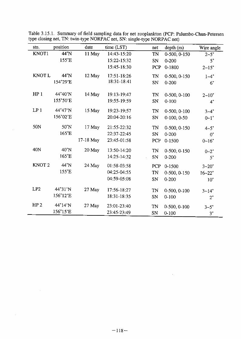
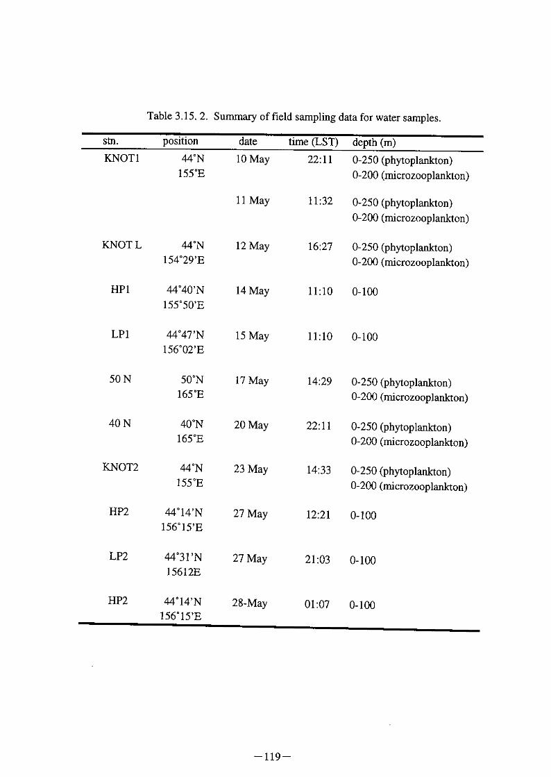
3.16 Atmospheric observation
3.16.1 Atmospheric input of iron over the Northwestern North Pacific Ocean.
Shigeto Nakabayashi
(Japan Marine Science and Technology Center)
(1) Introduction
Fe is one of the major elements in the earth's crust. However, its concentration
in seawater is extremely low. This low concentration is attributed to the fact that
solubility of thermodynamically stable Fe(III) is very low. In other wards, Fe in
seawater readily hydrolyzes to form insoluble colloidal hydrous ferric oxides, settling
down to the bottom. Because of this high reactivity, its residence time in the ocean is
one of the shortest, which is on the order of few hundreds years in deep water and
several weeks in surface water.
Fe has been also known as an essential micro-nutrient for the phytoplankton
growth in the ocean. Due to its extremely low solubility, however, the concentration
becomes so low that phytoplankton growth is subdued where its supply is limited.
Thus, the fate of Fe in seawater is closely related to the biological activity. It is very
important to know the behavior of Fe in the ocean for the study of the global
biogeochemical cycles of carbon and its related elements.
Fe is supplied from river and atmosphere to the ocean surface. However,
because of its rapid removal from seawater, riverine dissolved Fe is readily removed
within estuary, so that influence of riverine input to the open ocean surface may not be
recognized. Therefore the airborne dust has been proposed as a major source of
dissolved Fe to the open ocean surface.
The Northwestern North Pacific Ocean is characterized by upwelling of
deep water, high nutrients, high primary production and complicated water mass
structure (i.e. intermediate water), among others. And also large aeolian input of
terrigeneous material to the area is expected. Generally, in the North Pacific the
dominant source of the terrigeneous material is Asian dust. Because they can supply
Fe over the surface water, they have significant impact on the phytoplankton growth.
In addition, seasonal and geographical changes of these features are drastic. This
complexity has prevented us from knowing exactly to what extent it plays a role in the
global material cycles.
This study is focused on the impact of aeolian input to Fe distribution at the
surface water and phytoplankton growth in the Northwestern North Pacific Ocean.
(2) Methods
Atmospheric dust samples were collected for 24 hr. periods using a high volume
air sampler Model HVC-1000N (Shibata co.). The sampler was set up on the compass
deck with a wind sector control and filtered the air at the rate of about 1000 l min.-1.
21 atmospheric dust samples were collected on the 0.6 µm pore size Nuclepore
polycarbonate filters (203 x 253 mm) while the ship was steaming or at the stations.
After the collection of dust samples, the filters were kept in a freezer until its analysis
on the land-based laboratory. Samples collected in this cruise are listed in Table 1.
(3) Future plane
Atmospheric dust filter samples will be analyzed for iron and other metals by ICP-AES
or GFAAS after acid digestion. And also dissolution rate and solubility of
atmospheric Fe in seawater will be measured. Large aeolian input of terrigeneous
material (Asian dust) to the Northwestern North Pacific is expected. Because
they can supply Fe over the surface water, they have significant impact on the
phytoplankton growth. This study will be focused on the impact of aeolian input to Fe
distribution at the surface water and phytoplankton growth in this region.
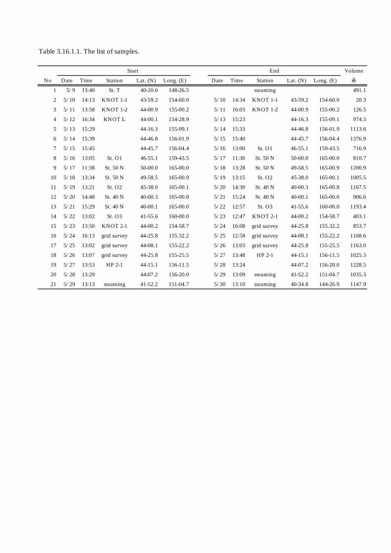
Table 3.16.1.1. The list of samples.
Start End Volume
No Date Time Station Lat. (N) Long. (E) Date Time Station Lat. (N) Long. (E) m
1 5/9 13:40 St. T 40-20.6 148-26.5 steaming 491.1
2 5/10 14:13 KNOT 1-1 43-59.2 154-60.0 5/10 14:34 KNOT 1-1 43-59.2 154-60.0 20.3
3 5/11 13:58 KNOT 1-2 44-00.9 155-00.2 5/11 16:03 KNOT 1-2 44-00.9 155-00.2 126.5
4 5/12 16:34 KNOT L 44-00.1 154-28.9 5/13 15:23 44-16.3 155-09.1 974.3
5 5/13 15:29 44-16.3 155-09.1 5/14 15:33 44-46.8 156-01.9 1113.6
6 5/14 15:39 44-46.8 156-01.9 5/15 15:40 44-45.7 156-04.4 1376.9
7 5/15 15:45 44-45.7 156-04.4 5/16 13:00 St. O1 46-55.1 159-43.5 716.9
8 5/16 13:05 St. O1 46-55.1 159-43.5 5/17 11:30 St. 50 N 50-00.0 165-00.0 810.7
9 5/17 11:38 St. 50 N 50-00.0 165-00.0 5/18 13:28 St. 50 N 49-58.5 165-00.9 1200.9
10 5/18 13:34 St. 50 N 49-58.5 165-00.9 5/19 13:15 St. O2 45-38.0 165-00.1 1005.5
11 5/19 13:21 St. O2 45-38.0 165-00.1 5/20 14:30 St. 40 N 40-00.3 165-00.8 1167.5
12 5/20 14:48 St. 40 N 40-00.3 165-00.8 5/21 15:24 St. 40 N 40-00.1 165-00.0 906.6
13 5/21 15:29 St. 40 N 40-00.1 165-00.0 5/22 12:57 St. O3 41-55.6 160-00.0 1193.4
14 5/22 13:02 St. O3 41-55.6 160-00.0 5/23 12:47 KNOT 2-1 44-00.2 154-58.7 403.1
15 5/23 13:50 KNOT 2-1 44-00.2 154-58.7 5/24 16:08 grid survey 44-25.8 155.32.2 853.7
16 5/24 16:13 grid survey 44-25.8 155.32.2 5/25 12:58 grid survey 44-08.1 155-22.2 1168.6
17 5/25 13:02 grid survey 44-08.1 155-22.2 5/26 13:03 grid survey 44-25.8 155-25.5 1163.0
18 5/26 13:07 grid survey 44-25.8 155-25.5 5/27 13:48 HP 2-1 44-15.1 156-11.5 1025.3
19 5/27 13:53 HP 2-1 44-15.1 156-11.5 5/28 13:24 44-07.2 156-20.0 1228.5
20 5/28 13:29 44-07.2 156-20.0 5/29 13:09 steaming 41-52.2 151-04.7 1035.3
21 5/29 13:13 steaming 41-52.2 151-04.7 5/30 13:10 steaming 40-34.8 144-26.9 1147.9
3
3.16.2 Atmospheric aerosol and ozone in the marine boundary layer
Kiyoshi Matsumoto and Mitsuo Uematsu
(Ocean Research Institute, The University of Tokyo)
(1) Introduction
Tropospheric aerosols are important in the global radiation budget through reflection and
absorption of solar radiation (direct forcing), and through the modification of optical properties and the
lifetime of clouds (indirect forcing). Global geographical and seasonal distributions of tropspheric
aerosols have attracted considerable attention during the past several decades. Especially, the importance
of the western North Pacific region has been recognized in the recent studies, due to the long-range
transport of anthropogenic and terrestrial aerosols from East Asia to the remote ocean.
In order to investigate the chemical and physical properties of marine aerosols over the western
North Pacific Ocean, the measurements of atmospheric aerosols have been carried out during this cruise.
Simultaneously, the concentration of ozone, which is a good indicator of air masses in marine boundary
layer, has been measured.
(2) Experimental
The measurements of carbonaceous aerosols were conducted for every 2 hours by using an
ambient carbon particulate monitor (Rupprecht & Patashnick Co. Inc., Model 5400). The instrument can
measure both the organic and elemental carbon in aerosols by a thermal analysis technique. Organic
carbon were measured by the combustion at 340°C, and then total carbon were measured at 750°C. The
difference of the amounts of the total and organic carbon gives the amount of elemental carbon.
Particle number concentrations were measured by using two particle counters (RION, Model KC-18 and
Model KC-01). The number concentrations of relatively small particles were measured by the KC-18
counter with 5 size ranges (0.10, 0.15, 0.20, 0.30, 0.50µm <d ) for every 10 min. On the other hand, those
of relatively large particles were measured by the KC-01 counter with 5 size ranges (0.30, 0.50, 1.0, 3.0,
5.0µm <d ) for every 20 min.
In this study, atmospheric aerosols only with diameter < 2.5µm were injected into the carbon
particulate monitor and the KC-18 counter by using PM2.5 cyclone (50% cutoff efficiency for 2.5µm
particle).
Ozone concentrations were measured at 12 seconds interval by an ozone analyzer (Dylec, Model 1150).
The inlets of air for the carbon particulate monitor, the ozone analyzer and the particle counters
were located on the compass deck (about 17m above the sea surface).
Bulk aerosol samples were collected for about 12 hour periods on cellulose acetate filters
(Whatman 41) by using a cassette high-volume aerosol sampler (Kimoto Co. Inc.), which is equipped
with automatic filter exchange system, and on cellulose acetate filters (Whatman 41) by a high-volume
aerosol sampler (Kimoto Co. Inc.). After collections, the samples were stored at ambient temperature
prior to analysis. Size-fractionated aerosols samples were collected for about 5 day periods on quartz fiber
filters (Pallflex 2500QAT-UP) by using an Andersen low pressure impactor (Tokyo Dylec, LP-20), which
can be segregated into 13 size fractions (50% effective cutoff diameter of each impactor stages are 0.06,
0.13, 0.21, 0.31, 0.51, 0.71, 1.2, 2.2, 3.6, 5.3, 8.0, 11µm.). Before sampling, quartz fiber filters have been
heated at 500°C for 4 hour. After collections, the samples were stored at -20°C prior to analysis. In order
to avoid contamination from the ship exhaust, aerosol samplers were automatically controlled by a wind
sector to start sampling only when the relative wind direction was within ± 90°C of the bow and the
relative wind speed was higher than 1.0m/s.
Rainwater samples were collected by using a rain sampler (Shibata Co., W-102) with in-situ
filtration by each rain event basis. After collections, the value of pH and electrical conductivity were
measured immediately, and then the samples were stored in polypropylene bottles at 4°C.
The collections of aerosol and rainwater were carried out on the compass deck.
(3) Preliminary Results
Ozone
The concentrations of ozone during the cruise are shown in Figure 3.16.2.1. Relatively high
concentrations were detected throughout the cruise, since the present research area is higher latitudinal
oceanic region. Due to the anthropogenic effects, the concentrations increased near the Japan Islands.
During 21-22 May, drastic decrease of ozone concentrations were detected, probably due to the invasion
of subtropical air mass, of which ozone concentrations generally show lower values, accompany with
movement of the low pressure system to the north.
Carbonaceous aerosols
The concentrations of particulate organic and elemental carbon are shown in Figure 3.16.2.2
Both revealed lower concentrations over the remote oceanic region, whereas enhanced concentrations of
both can be seen near the Japan Island, showing anthropogenic effects.
(3) Future Plan
Bulk aerosol samples and rainwater samples will be analyzed for major inorganic ions.
Size-fractionated aerosol samples will be analyzed for organic compounds. After the determination of
data quality, the separation of air masses will be attempted by the meteorological data observed on the
ship. It may be possible to discuss the geographical characteristics of the chemical properties of
atmospheric aerosols and the influence of air mass history and meteorological conditions to the aerosol
chemistry over the western North Pacific Ocean.
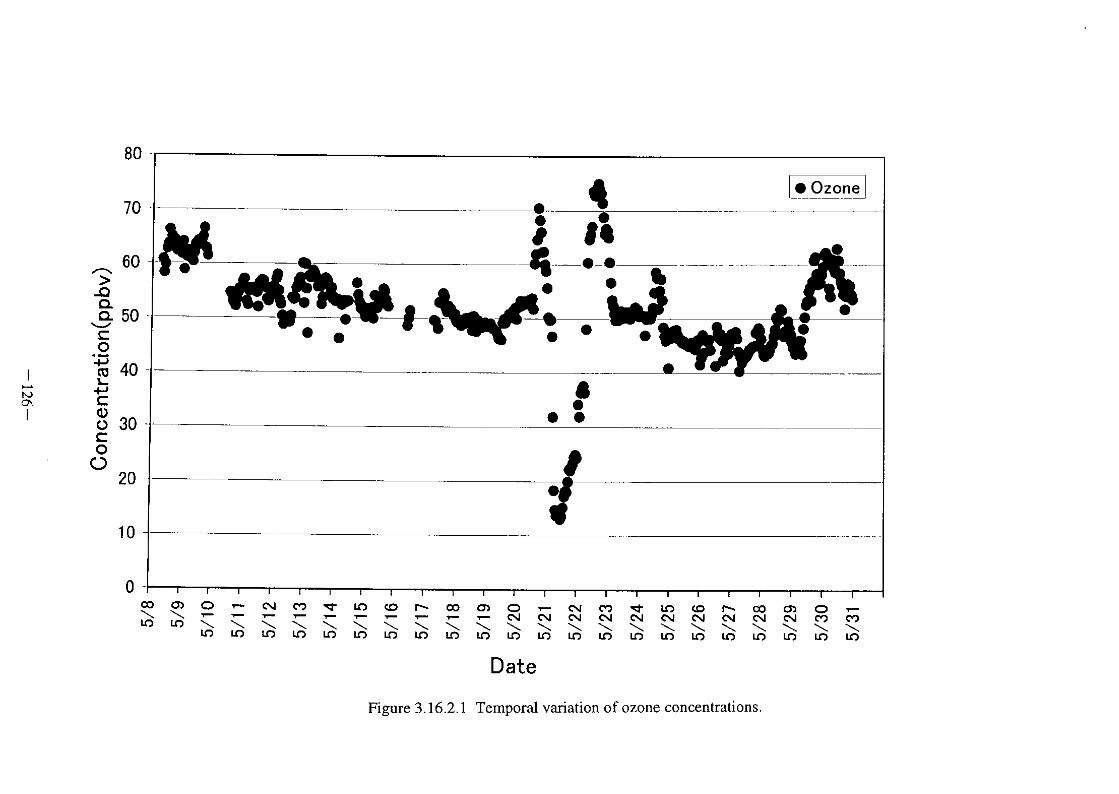

3.16.3 Nonmethane hydrocarbons and ozone measurements over the western North Pacific
Takuya Saito, Masahiro Narukawa and Kimitaka Kawamura
(Institute of Low Temperature Science, Hokkaido University)
(1) Introduction
Recently, it has been discussed that halogen atoms may be of considerable importance for the
tropospheric chemistry. They may affect the oxidizing capacity of the atmosphere, especially, the
atmospheric removal rate of nonmethane hydrocarbons (NMHCs) and ozone. However, presently there is
no method which allow the direct measurement of halogen atoms. Consequently, the evidence for the
existence of relevant levels of halogen atoms is only indirect. Logarithmic plots of the ratios of
hydrocarbon concentrations are such an indirect method to gain insight into their reactions with halogen
atoms, especially, chlorine atoms.
For a few atmospheric trace gases, concentration measurements have been complemented by
determinations of their isotopic composition. Such information has provided additional constr a i n t s o n
b u d g e t s a n d r e m o v a l m e c h a n i s m . A l t h o u g h v e r y f e w m e a s u r e m e n t s o f i s o t o p i c
c o m p o s i t i o n a r e a v a i l a b l e f o r N M H C s , t h e i s o t o p i c c o m p o s i t i o n ( δ1 3 C ) o f N M H C s
m a y b e a v e r y v a l u a b l e t r a c e r f o r b e t t e r u n d e r s t a n d i n g o f c h l o r i n e a t o m c h e m i s t r y
i n t h e t r o p o sphere.
(2) Methods
Air samples (n=45) were collected on the compass deck of R/V Mirai by pressurizing the
stainless canisters with metal bellows pump to about 1.5 atm. Tropospheric ozone was measured every 12
seconds by an ozone monitor (Dylec, 1150). The air was drawn through a Teflon line (1/4' OD) using a
pump. The air intake was located on compass deck.
(3) Future plan
The sample analysis will be made in the laboratory for NMHCs. NMHCs in the canister will be
concentrated using a preconcentration unit a n d m e a s u r e d u s i n g a G C e q u i p p e d w i t h a f l a m e
i o n i z a t i o n d e t e c t o r . M e a s u r e m e n t s o f δ1 3 C o f N M H C s w i l l b e m a d e b y i s o t o p e r a t i o m a s s
s p e c t r o m e t e r ( I R M S ) i n t e r f a c e d t o a c a p i l l a r y g a s c h r o m a t o g r a p h a n d o n - l i n e c o m b u s t i o n
s y s t e m . A f t e r t h e d e t e r m i n a t i o n o f d a ta quality, these data will be used to investigate the possible
impact of chlorine atom on the removal processes of NMHCs over the western North Pacific.

3.16.4 Organic aerosols over the western North Pacific
Masahiro Narukawa and Kimitaka Kawamura
(Institute of Low Temperature Science, Hokkaido University)
(1) Introduction
For marine organic aerosol study, western North Pacific is an interesting oceanic region. During
spring season, transport of anthropogenic and terrestrial materials from East Asian continent is intensified
and the spring blooms of phytoplankton occur in this region. An intensified transport of organic
compounds to the marine environments as well as sea-to-air flux of volatile and particulate materials from
the ocean change the composition of marine aerosols, and may have an influence on the optical and
microphysical properties of clouds in the western North Pacific.
Previous studies on the marine organic aerosols have shown that water-soluble organic acids including
low molecular weight dicarboxylic acids are abundant in the marine aerosols (Kawamura and Usukura,
1993). They comprise up to 18% of the total aerosol carbon in the Pacific atmosphere and their latitudinal
distribution suggested that the low molecular weight diacids are produced in the marine atmosphere by
photochemical oxidation of various organic compounds, mostly light hydrocarbons and
oxygen-containing organic compounds (Kawamura and Sakaguchi, 1999). Further, water-soluble
organics alter hygroscopic behavior of atmospheric particles, suggesting that water-soluble organic
compounds play an important role in controlling cloud albedo by acting as CCN. The cloud activity may
compensate the potential global warming caused by the increased concentrations of greenhouse gases
such as carbon dioxide.
Properties of aerosols depend on the size distribution as well as chemical composition. The aim of our
studies in this expedition is to clarify the size distribution of low molecular weight dicarboxylic acids and
their spatial distributions.
(2) Samples
Marine aerosol samples were collected on compass deck of R/V Mirai using a pre-combusted
(450°C, 3 h o u r s ) q u a r t z f i b e r f i l t e r ( P a l l f l e x , 2 5 0 0 Q A T - U P ) a n d h i g h v o l u m e a i r s a m p l e r
( K i m o t o , 1 2 0 F ) o r h i g h v o l u m e a i r s a m p l e r w i t h A n d e r s e n t y p e 5 - s t a g e i m p a c t o r ( S h i b a t a ,
H V C - 1 0 0 0 N ) . F i l t e r s a m p l e s w e r e s t o r e d i n a p r e - c l e a n e d g l a s s j a r w i t h a T e f l o n - l i n e d s c r e w
c a p a t 2 0°C p r i o r t o a n a l y s i s . R a i n w a t e r s a m p l e s w e r e a l s o c o l l e c t e d u s i n g a s t a i n l e s s s t e e l
r a i n c o l l e c t o r . T h e r a i n s a m p l e s w e r e s t o r e d i n a b r o w n - c o l o r e d g l a s s b o t t l e w i t h a
T e f l o n - l i n e d s c r e w c a p , t o w h i c h s m a l l a m o u n t o f HgCl2 w a s a d d e d a s b a c t e ricide.
(3) Future Plan
Aerosol samples will be analyzed for low molecular weight diacids. Aliquots of aerosol filter
samples will be extracted with pure water for the isolation of dicarboxylic acids. The extracts will be
concentrated and then esterified with 14% borontrifluoride in n-butanol to derive dicarboxylic acid
dibutyl esters. The esters will be determined using a GC and GC/mass spectrometer.
Based on the size distribution of diacids, we will estimate relative contribution of the continental
and marine source inputs to diacids in the marine aerosols. Comparison of this study with the previous
study also may characterize the aerosols in this region during spring season.
References
Peltzer, E. T. and R. B. Gagosian, Organic geochemistry of aerosols over the Pacific Ocean, in Chemical
Oceanography Vol. 10, pp.281-338, Ed. J. P. Riley, R. Chester and R. A. Duce, Academic Press, London,
UK, 1989.
Kawamura, K. and K. Usukura, Distribution of low molecular weight dicarboxylic acids in the North
Pacific aerosol samples, J. Oceanogr., 49, 271-283, 1993.
Kawamura, K. and F. Sakaguchi, Molecular distributions of water soluble carboxylic acids in marine
aerosols over the Pacific Ocean including tropics, J. Geophys. Res., 104, 3501-3509, 1999.

3.17 Underway observation 3.17.1 Partial pressure of CO2 (pCO2) in the atmosphere and sea surface
Akihiko Murata (JAMSTEC)
Mikio Kitada (MWJ)
Concentrations of CO2 in the atmosphere and the sea surface were measured
continuously during the entire cruise by the automated system with a non-
dispersive infrared (NDIR) analyzer (BINOSTM). It runs on half hour or two hours
cycle during which four standards, an ambient air sample, and a head space sample
from the equilibrator were analyzed.
The ambient air sample taken from the bow is introduced into the NDIR
through a mass flow controller which controls the air flow rate at about 0.5L/min, a
cooling unit, a perma pure dryer, and a desiccant holder (Mg(ClO4)2).
The equilibrator has shower head space in the top through which surface water
is forced at a rate of 5-8L/min. Air in the head space is circulated with an air pump
at 0.5-0.8L/min in a closed loop through two cooling units, a perma pure dryer, and
the desiccant holder.
For calibration, compressed gas standards with nominal mixing ratios of 270,
330, 360, 410, ppmv (parts per million by volume) were used.
In this cruise, measurement of discrete pCO2 was also tested. From this test,
it was found that ratio of air to seawater in an equilibrator should be changed for
more efficient equilibration.
3.17.2 Measurement of CO2 in the atmosphere and in surface seawater
Takeshi Egashira
(Japan Science and Technology Corporation)
(1) Introduction
Concentrations of the partial pressure of CO2 (pCO2) in surface seawater were measured
continuously during the cruise. T h e r e w e r e t h r e e p r i m a r y o b j e c t i v e s o f t h e c r u i s e . F i r s t w a s t o a s s e s s
p CO2
a t t h e s t a t i o n K N O T . S e c o n d w a s t o m e a s u r e p CO2 d u r i n g t h e c r u i s e . T h i r d w a s t o discover
occuring bloom.
(2) M e t h o d s
S u r f a c e s e a w a t e r i s p u m p e d u p t o a T a n d e m - s t y l e e q u i l i b r a t o r ( K i m o t o E l e c t r i c C o . , L t d . ) a n d t h e
g a s e s w e r e e q u i l i b r a t e d w i t h a h e a d s p a c e o f t h e e q u i l i b r a t o r . A f t e r e q u i l i b r a t i o n t h e h e a d s p a c e g a s w a s d r i e d
a n d a n a l y z e d u s i n g a s t a n d a r d i z e d i n f r a - r e d a n a l y z e r . T h e p CO2 i n s u r f a c e s e a w a t e r w a s m e a s u r e d u s i n g t h e
i n f r a - r e d a n a l y z e r w i t h a n e s t i m a t e d p r e c i s i o n o f a p p r o x i m a t e l y 0 . 0 5 p p m .
(3) F u t u r e p l a n
We have three plans for pCO2 data. First is to add GPS, atmospheric pressure, seawater
temperature, and salinity data. Second is to correct data with salinity, pressure, and warming. Third is
to extract and assess data around station KNOT.
3 . 1 7 . 3 Salinity, temperature, DO, and fluorescence
N o b u h a r u K o m a i , K a t s u n o r i S a g i s h i m a
( M a r i n e W o r k s J a p a n L t d . )
H a j i m e K a w a k a m i
( J a p a n M a r i n e S c i e n c e a n d T e c h n o l o g y C e n t e r )
( 1 ) I n t r o d u c t i o n
T o m o n i t o r c o n t i n u o u s l y t h e p h y s i c a l , c h e m i c a l a n d b i o l o g i c a l c haracteristic of sea surface water
and to find the bloom during this cruise.
(2) Methods
The Continuous Sea Surface Water Monitoring System is located in the "sea surface monitoring
laboratory" on R/V Mirai. It can automatically measure temperature, salinity, dissolved oxygen,
fluorescence and particle size of plankton in the surface water every one minute. Measured data are saved
every one minute together with time and the position of ship, and displayed in the data management PC
machine. This system is connected to shipboard LAN-system and provides the acquired data for pCO2
measurement system, etc.
Sea surface water was continuously pumped up from the seachest of the ship at 4 meters depth to
the laboratory and then flowed into the Continuous Sea Surface Water Monitoring System and pCO2
measurement system etc. through a steel pipe. The flow rate of surface water for the Continuous Sea
Surface Water Monitoring System was controlled by some valves and passed through some sensors i.e.
temperature, salinity and dissolved oxygen etc. through vinyl-chloride pipes. At this cruise, the picture of
PC machine were showed to TV monitor of the ship. Mr. Furuta of GODI did it for us.
This system have six kinds of sensor, specification and calibration date of the each sensors are
listed below.
a-1) Temperature and salinity sensors
SEACAT THERMOSALINOGRAPH
Model: SBE-21, SEA-BIRD ELECTRONICS, INC.
Serial number: 2113117-2088
Measurement range: Temperature -5 to +35 deg-C, Salinity 0 to 6.5 S/m
Accuracy: Temperature 0.01 deg-C/6month, Salinity 0.001 S/m/month
Resolution: Temperature 0.001 deg-C, Salinity 0.0001 S/m
Calibration date: 09-Jan-99 (mounted on 5-May-99 in this system)
a-2) Ship bottom oceanographic thermometer (mounted at the back of the pump for surface water)
Model: SBE 3S, SEA-BIRD ELECTRONICS, INC.
Serial number: 032175
Measurement range: -5 to +35 deg-C
Initial Accuracy: 0.001 deg-C per year typical
Stability: 0.002 deg-C per year typical
Calibration date: 30-Dec-98 (mounted on 23-Apr-99 in this system)
b) Dissolved oxygen sensor
Model: 2127, Oubisufair Laboratories Japan INC.
Serial number: 31757
Measurement range: 0 to 14 ppm
Accuracy: ±1% at 5 deg-C of correction range
Stability: 1% per month
Calibration date: 7-May-99
c) Fluorometer
Model: 10-AU-005, TURNER DESIGNS
Serial number: 5562 FRXX
Detection limit: 5 ppt or less for chlorophyll a
Stability: 0.5% per month of full scale
d) Particle size sensor
Model: P-05, Nippon Kaiyo LTD.
Serial number: P5024
Accuracy: ±10% of range
Measurement range: 0.02681mm to 6.666mm
Reproducibility: ±5%
Stability: 5% per week
e) Flowmeter
Model: EMARG2W, Aichi Watch Electronics LTD.
Serial number: 8672
Measurement range: 0 to 30 L/min
Accuracy: ±1%
Stability: ±1% per day
(3) Preliminary Result
In order to calibrate the data from this system, seawater samples were collected from the system.
For salinity validation we sampled once a day from the system during this cruise (except with the
18-May-99). All salinity samples were analyzed by an Autosal salinometer (see section 3.3.3) and the
results were shown in table 3.17.3-1.

We compared salinity values of the water samples and those from SBE21 sensor of the system
(Fig. 3.17.3-1). There was not a constant trend of difference during this cruise. We calculated the Root
Mean Squares (R.M.S.) of difference of salinity value for 19 samples and it was 0.0178 (one sigma)
except with the data which difference was ca.1PSU.
D.O. sensor of this system was calibrated just before this cruise. To estimate of accuracy of the
sensor, we collected the 10 samples from the course of the system and analyzed by Winkler method (see
section 3.3.1). The results were shown in table 3.17.3-2 and Fig. 3.17.3-2. Calculated R.M.S. of
differences of D.O. value was 0.255 ml/l (one sigma).
Preliminary data every 10 minutes from Sekinehama to Stn. KNOT, Stn. KNOT to Stn. 50N, Stn.
50N to Stn. 40N, Stn. 40N to Stn. KNOT2, Stn. KNOT2 to sekinehama were shown in Fig. 3.17.3-3 ~ F i g .
3 . 1 7 . 3 - 7 , r e s p e c t i v e l y . T h e y s h o w e d t h e r e s p e c t i v e t r e n d o f t e m p e r a t u r e , s a l i n i t y , D . O . a n d f l u o r e s c e n c e d i s t r i
b u t i o n s o n t h e s h i p ' s t r a c k .
( 4 ) O t h e r r e m a r k s
T h e d a t a f r o m t h e p a r t i c l e s i z e s e n s o r w e r e n o t r e l i a b l e , b e c a u s e t h e s e t t i n g o f t h e s e n s or was not
good. We cleaned the flow cell of fluorometer at Sekinehama just before this cruise.
(5) Data archive
All the files of raw data, Microsoft excel files of raw data, excel files divided into each
10minutes data were stored on a magnetic optical disk. All the data will be submitted to the DMO at
JAMSTEC.

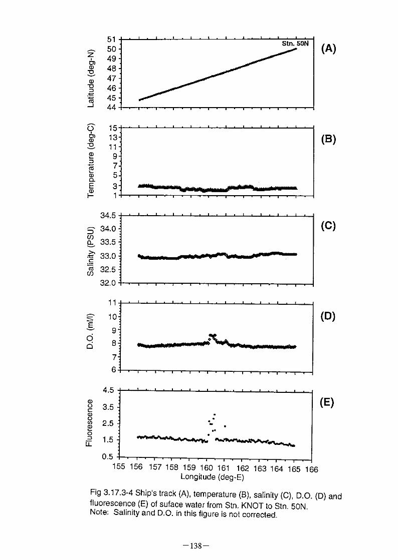
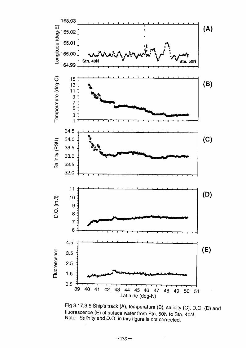
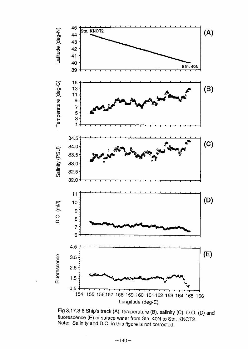
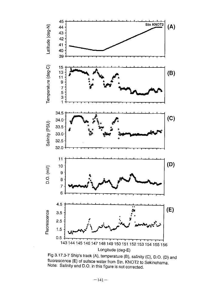

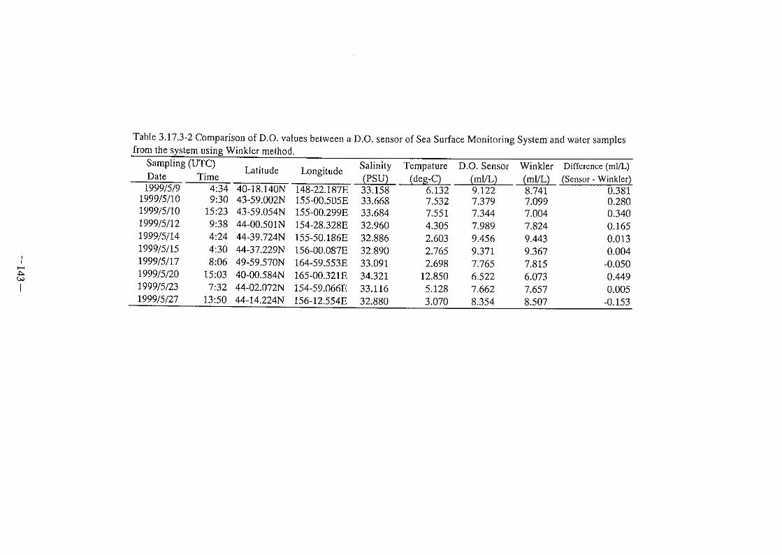
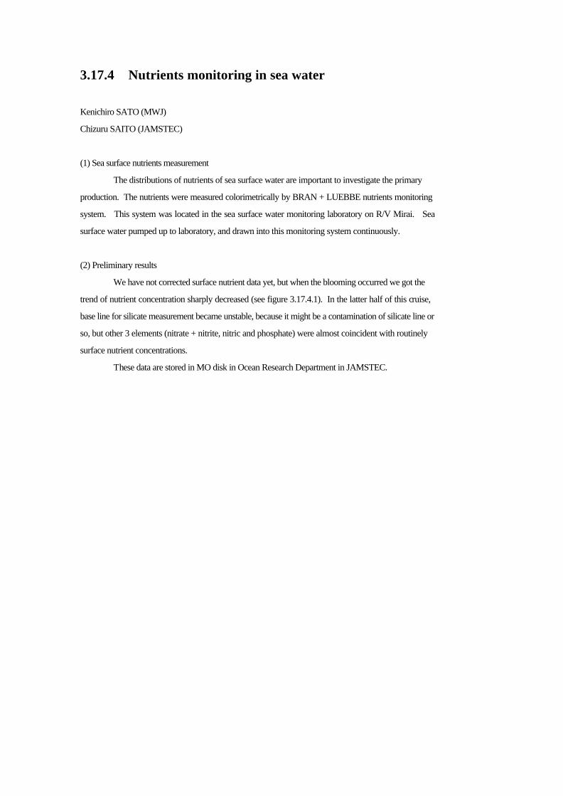
3.17.4 Nutrients monitoring in sea water
Kenichiro SATO (MWJ)
Chizuru SAITO (JAMSTEC)
(1) Sea surface nutrients measurement
The distributions of nutrients of sea surface water are important to investigate the primary
production. The nutrients were measured colorimetrically by BRAN + LUEBBE nutrients monitoring
system. This system was located in the sea surface water monitoring laboratory on R/V Mirai. Sea
surface water pumped up to laboratory, and drawn into this monitoring system continuously.
(2) Preliminary results
We have not corrected surface nutrient data yet, but when the blooming occurred we got the
trend of nutrient concentration sharply decreased (see figure 3.17.4.1). In the latter half of this cruise,
base line for silicate measurement became unstable, because it might be a contamination of silicate line or
so, but other 3 elements (nitrate + nitrite, nitric and phosphate) were almost coincident with routinely
surface nutrient concentrations.
These data are stored in MO disk in Ocean Research Department in JAMSTEC.
3.18 Sea floor sediment sampling and study on geochemical cycle on sea floor
Koh Harada (National Institute for Resources and Environment)
Yoko Shibamoto (National Institute for Resources and Environment)
Toshikatsu Sugawara (Marine Works Japan Ltd.)
(1) Introduction
Water-sediment boundary is a place where biogeochemical processes actively
occur. To clarify regeneration process of nutrients, balances of the
nutrients at the boundary are investigated by measuring the nutrient
concentration in pore water.
Sediment particles near the boundary are well mixed by organisms at sea
floor. To clarify the space and seasonal variation of the bioturbation,
shot lived radio-nuclides are also investigated.
(2) Methods and preliminary result
Sediment core sampling were conducted at two stations, STN 50N and STN
KNOT-2 using with a Multiple Corer. The coring logs are shown in Table 3.18.1. Eight
non-disturbed cores of which length was about 30 cm were successively collected at both stations.
Immediately after recovering the corer on the deck, four of the eight cores from each station were sliced
in about 3.5 mm thick each for topmost ten
sub-samples, about 7 mm thick each for the next ten sub-samples and about 14
mm thick each for other sub-samples down to the bottom. Pore water samples
were squeezed by centrifugation at 2oC from sub-samples of the two cores.
Concentrations of silicate, phosphate, nitrate and nitrite were determined
by an Auto Analyzer.
Sub-samples from the another three cores at STN 50N and two cores at STN
KNOT-2 were kept in a freezer and brought to the land laboratory in NIRE.
Concentrations of 234Th, 210Pb and 210Po will be determined. For general
information of the geochemical properties, water content, concentration of
CaCO3, biogenic silica and sedimentation rate by 230Th method will be also
investigated. The vertical profiles of the water content were shown in
Fig. 3.18.1.
Core description was drawn from one non-sliced core. X-ray photographs were
also taken from the same core. The core descriptions were shown in Fig. 3.18.2.
Other cores were distributed as follows:
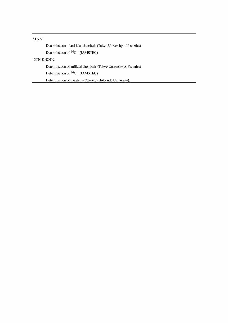
STN 50
Determination of artificial chemicals (Tokyo University of Fisheries)
Determination of 14C (JAMSTEC)
STN KNOT-2
Determination of artificial chemicals (Tokyo University of Fisheries)
Determination of 14C (JAMSTEC)
Determination of metals by ICP-MS (Hokkaido University).
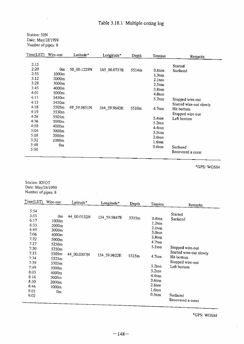

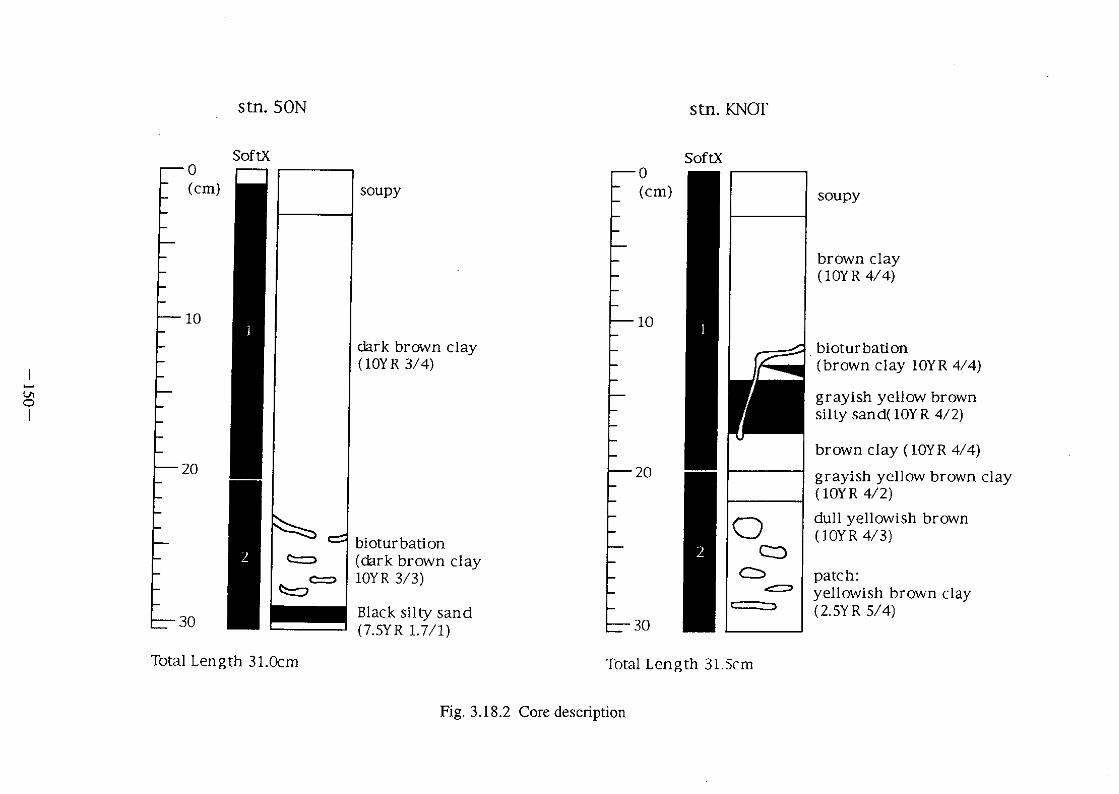
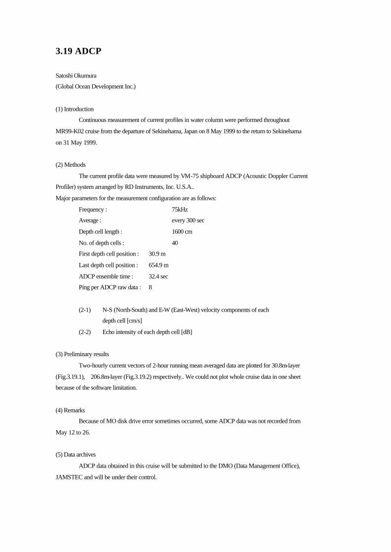
3.19 ADCP
Satoshi Okumura
(Global Ocean Development Inc.)
(1) Introduction
Continuous measurement of current profiles in water column were performed throughout
MR99-K02 cruise from the departure of Sekinehama, Japan on 8 May 1999 to the return to Sekinehama
on 31 May 1999.
(2) Methods
The current profile data were measured by VM-75 shipboard ADCP (Acoustic Doppler Current
Profiler) system arranged by RD Instruments, Inc. U.S.A..
Major parameters for the measurement configuration are as follows:
Frequency : 75kHz
Average : every 300 sec
Depth cell length : 1600 cm
No. of depth cells : 40
First depth cell position : 30.9 m
Last depth cell position : 654.9 m
ADCP ensemble time : 32.4 sec
Ping per ADCP raw data : 8
(2-1) N-S (North-South) and E-W (East-West) velocity components of each
depth cell [cm/s]
(2-2) Echo intensity of each depth cell [dB]
(3) Preliminary results
Two-hourly current vectors of 2-hour running mean averaged data are plotted for 30.8m-layer
(Fig.3.19.1), 206.8m-layer (Fig.3.19.2) respectively.. We could not plot whole cruise data in one sheet
because of the software limitation.
(4) Remarks
Because of MO disk drive error sometimes occurred, some ADCP data was not recorded from
May 12 to 26.
(5) Data archives
ADCP data obtained in this cruise will be submitted to the DMO (Data Management Office),
JAMSTEC and will be under their control.

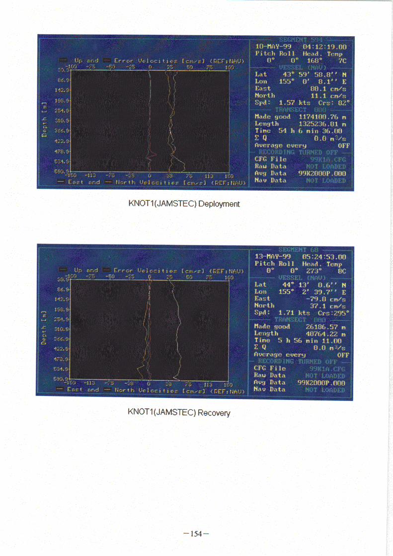
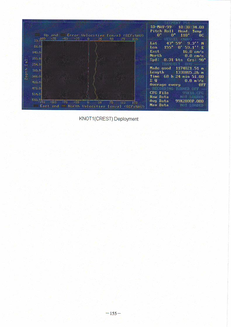
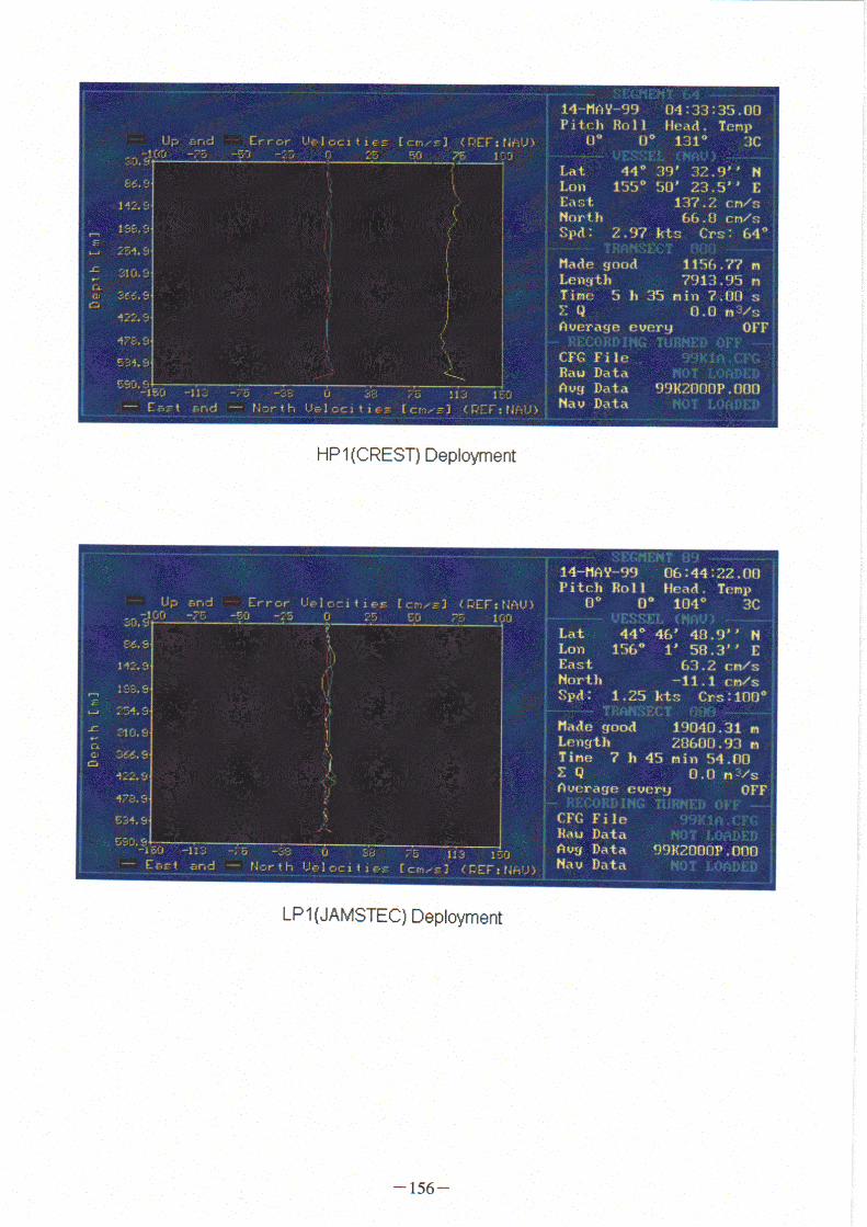
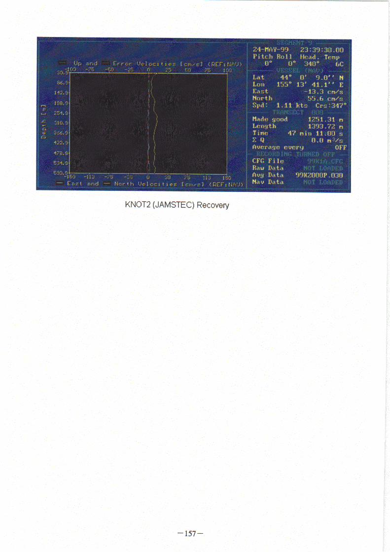
3.20 Underway Geophysics 3.20.1 Multi-Narrow Beam Echo Sounding System
Toshio Furuta and Satoshi Okumura (GODI)
(1) Introduction
R/V Mirai has installed a multi narrow beam echo sounding system manufactured by SeaBeam
Inc., SeaBeam 2100 system. This system utilized bathymetry mapping and subbottom profiler. The
newest one can measure more than 120 degrees wider swath and available all depth of the world ocean
floor.
(2) System configuration
The system consists of mainly four segments; under hull unit, controller electronic circuits, real
time display unit, and post processing unit. Under hull unit has two projector alleys, one is for 12kHz
and another for 4kHz with one hydrophone alley. The hydrophone alley can receive both returning
acoustic signals of 12kHz and 4kHz, interleavingly. Main electronic circuits of 12kHz bathymetry and
4kHz subbottom profiler have the individual consoles in which the cpus and dsp boards process receiving
signals. The real time display unit consists of three Indy workstations (W/S), two of them are for 12kHz
terminal and real time display, and one for subbottom profiling controller. The system has also output
devices such as graphic recorders, color printer and color plotter.
(3) Method
Gridding survey in this cruise was carried out on the three sites at 44° N, 155E° (KNOT site),
50° N and 40°N along 165°E. Each area is approximately 60 n.m. square or less, and depth from 5800m
to 3000m. The gridding survey interval being one and half or twice of depth is different depending on
their depths. After the gridding survey, the bathymetric data were fed to post processing W/S by ftp
command. The post processing system furnished on this MNBES has two high performance W/S
Indigo2 which have "mb-system" software on the basis of the Genetic Mapping Tool (GMT) called
SeaView. Consequently, measured data can easily be edited on W/S by automatically or manually to
provide gridding data and map images.
The bathymetry data gridding on the basis of netCDF format can be sent to the network server of
Mirai to overprint on the navigation track display.
(4) Results
It is, of course, required to keep high accuracy that precise correction of sound speed of the
target area can be performed based on the temperature profiles of water column. During this cruise,
CTD casts have done at the target sites or very close to the sites, we could obtain the sound velocity
profile derived from the CTD data. The newest system has continuously measured the surface water

sound velocity in real time, because sound velocity at the hydrophone alley is a very important factor to
determine the angle of acoustic ray path which affects the outer beam of wider swath.
Figures 3.20.3-1 to 3.20.3-3 show the bathymetric topographies of survey areas, these are drown
in addition to the previous data which were measured MR98-K01 or older scientific cruises.
(5) Data storage
Media; Exabyte tape
Place: JAMSTEC Data Management Office and JODC of Japan Marine Safety
Agency


3.20.2. Sea Surface Gravity
Toshio Furuta and Satoshi Okumura (GODI)
(1) Introduction
Sea Surface gravity measurement during MR99-K02 cruise using a LaCoste-Romberg gravity
meter S-116 installed on the R/V Mirai among port call of Sekinehama.
(2) System configuration
The system consists of three components, first is a sensor platform with horizontally stabilized
mechanism(two axes of gyros and torque motors), second is a digital control system, and third is a
cataloging PC which can record data in 3.5" optical magnetic disk (MO) at every ten second in addition
with common navigation information. Data is also sent to the Mirai network server through ethernet
LAN system via terminal server.
(3)Method
As system can measure only the relative variation of gravity values, the value were correlated by
the absolute or known gravity values at each port (from start to finish of one cruise or leg). Moreover,
measured values are corrected based on the bathymetry(free-air) and ship movement(etoveth).
Consequently, the corrected gravity data should involve the information of crustal and upper mantle
structures how they compensate the discrepancy from isostatic balance.
(4) Data storage:
Media; 3.5" magnetic optical disk (230MB MO)
Place; JAMSTEC Data Management Office
Annex shows the observed values at Sekinehama gravity base measured by a Scintrex gravity
meter CG-3M, these values were used for correction of sea surface gravity meter at the ports.
3.20.3. Surface three component magnetometer
Toshio Furuta and Satoshi Okumura (GODI)
(1)Introduction
In order to continuously obtain the geomagnetic field vectors on the sea surface, a three
component magnetometer is a very useful equipment. The magnetic force on the sea is affected by
induction of magnetized body beneath the subbottom in addition to the earth dipole magnetic field.
The magnetic measurement on the sea is, therefore, one of utilities for geophysical reconstruction of
crustal structure and so on. The geomagnetic field can be divided into three components, i.e., two
horizontal (x & y)and one vertical (z) moments. Three-component observation instead of total force
includes much information of magnetic structure of magnetized bodies.
(2) System configuration
The system is mainly divided into three segments; sensor unit, control and datalogging unit, and
gyro and vertical reference unit (VRU). The sensor unit is installed on the top of foremast, the control
and datalogging unit in the dry laboratory, and the VRU also in dry lab. The gyro(ship heading) using
this system is as same as navigation gyrocompass. A ring laser gyro in the Doppler Radar Meteorology
system can be used to measure the ship attituide, instead of normal VRU, because of high precision
(3) Method
The sensor is a three axes fluxgate magnetometer and sampling period is 8Hz. The timing of
sampling is controlled by the 1pps standard clock of GPS signal. Every one second data set which
consists of 310 bytes; navigation information, 8 Hz three component of magnetic forces and ship's
attitude data were recorded in the external hard disk. The data set is simultaneously fed to the Mirai
network server through ethernet LAN system.
(4) Results
During MR99-K02 cruise, the magnetic force is continuously measured among port call of
Sekinehama. Data obtained on the sea will be analyzed in near future.
The procedure of quality control of the measured data is mainly to eliminate the effect of ship's
magnetized vector condition.
(5) Data storage:
Media; 3.5" optical magnetic disk(230MB MO)
Place; JAMSTEC Data Management Office