MPEG Tektronix
64
7/16/2019 MPEG Tektronix http://slidepdf.com/reader/full/mpeg-tektronix 1/64 A Guide to MPEG Fundamentals and Protocol Analysis (Including DVB and ATSC)
Transcript of MPEG Tektronix
7/16/2019 MPEG Tektronix
http://slidepdf.com/reader/full/mpeg-tektronix 1/64
A Guide to MPEG Fundamentals and Protocol Analysis(Including DVB and ATSC)

7/16/2019 MPEG Tektronix
http://slidepdf.com/reader/full/mpeg-tektronix 2/64
7/16/2019 MPEG Tektronix
http://slidepdf.com/reader/full/mpeg-tektronix 3/64
A Guide to MPEG Fundamentals
and Protocol Analysis(Including DVB and ATSC)

7/16/2019 MPEG Tektronix
http://slidepdf.com/reader/full/mpeg-tektronix 4/64
ii
A Guide to MPEG Fundamentals and Protocol Analysis
www.tektronix.com/video_audio/
7/16/2019 MPEG Tektronix
http://slidepdf.com/reader/full/mpeg-tektronix 5/64
A Guide to MPEG Fundamentals and Protocol Analysis
www.tektronix.com/video_audio/ iiiiiiiii
Section 1 – Introduction to MPEG · · · · · · · · · · · · · · · · · · · · · · · · · · · · 1
1.1 Convergence · · · · · · · · · · · · · · · · · · · · · · · · · · · · · · · · · · · · · · · · · · · · · · · · · · · · · · 1
1.2 Why Compression is Needed · · · · · · · · · · · · · · · · · · · · · · · · · · · · · · · · · · · · · · · · · · 1
1.3 Applications of Compression · · · · · · · · · · · · · · · · · · · · · · · · · · · · · · · · · · · · · · · · · · 1
1.4 Introduction to Video Compression · · · · · · · · · · · · · · · · · · · · · · · · · · · · · · · · · · · · 2
1.5 Introduction to Audio Compression · · · · · · · · · · · · · · · · · · · · · · · · · · · · · · · · · · · · · 4
1.6 MPEG Signals · · · · · · · · · · · · · · · · · · · · · · · · · · · · · · · · · · · · · · · · · · · · · · · · · · · · · 4
1.7 Need for Monitoring and Analysis · · · · · · · · · · · · · · · · · · · · · · · · · · · · · · · · · · · · · · 5
1.8 Pitfalls of Compression · · · · · · · · · · · · · · · · · · · · · · · · · · · · · · · · · · · · · · · · · · · · · · 6
Section 2 – Compression in Video· · · · · · · · · · · · · · · · · · · · · · · · · · · · 7
2.1 Spatial or Temporal Coding? · · · · · · · · · · · · · · · · · · · · · · · · · · · · · · · · · · · · · · · · · · 7
2.2 Spatial Coding · · · · · · · · · · · · · · · · · · · · · · · · · · · · · · · · · · · · · · · · · · · · · · · · · · · · 7
2.3 Weighting · · · · · · · · · · · · · · · · · · · · · · · · · · · · · · · · · · · · · · · · · · · · · · · · · · · · · · · · 9
2.4 Scanning · · · · · · · · · · · · · · · · · · · · · · · · · · · · · · · · · · · · · · · · · · · · · · · · · · · · · · · · 10
2.5 Entropy Coding · · · · · · · · · · · · · · · · · · · · · · · · · · · · · · · · · · · · · · · · · · · · · · · · · · · 10
2.6 A Spatial Coder · · · · · · · · · · · · · · · · · · · · · · · · · · · · · · · · · · · · · · · · · · · · · · · · · · · 11
2.7 Temporal Coding · · · · · · · · · · · · · · · · · · · · · · · · · · · · · · · · · · · · · · · · · · · · · · · · · · 12
2.8 Motion Compensation · · · · · · · · · · · · · · · · · · · · · · · · · · · · · · · · · · · · · · · · · · · · · · 13
2.9 Bidirectional Coding · · · · · · · · · · · · · · · · · · · · · · · · · · · · · · · · · · · · · · · · · · · · · · · 15
2.10 I, P, and B Pictures · · · · · · · · · · · · · · · · · · · · · · · · · · · · · · · · · · · · · · · · · · · · · · · 152.11 An MPEG Compressor · · · · · · · · · · · · · · · · · · · · · · · · · · · · · · · · · · · · · · · · · · · · · 17
2.12 Preprocessing · · · · · · · · · · · · · · · · · · · · · · · · · · · · · · · · · · · · · · · · · · · · · · · · · · 20
2.13 Profiles and Levels · · · · · · · · · · · · · · · · · · · · · · · · · · · · · · · · · · · · · · · · · · · · · · · 21
2.14 Wavelets · · · · · · · · · · · · · · · · · · · · · · · · · · · · · · · · · · · · · · · · · · · · · · · · · · · · · · · 22
Section 3 – Audio Compression · · · · · · · · · · · · · · · · · · · · · · · · · · · · 23
3.1 The Hearing Mechanism · · · · · · · · · · · · · · · · · · · · · · · · · · · · · · · · · · · · · · · · · · · · 23
3.2 Subband Coding · · · · · · · · · · · · · · · · · · · · · · · · · · · · · · · · · · · · · · · · · · · · · · · · · · 24
3.3 MPEG Layer 1 · · · · · · · · · · · · · · · · · · · · · · · · · · · · · · · · · · · · · · · · · · · · · · · · · · · · 25
3.4 MPEG Layer 2 · · · · · · · · · · · · · · · · · · · · · · · · · · · · · · · · · · · · · · · · · · · · · · · · · · · · 26
3.5 Transform Coding · · · · · · · · · · · · · · · · · · · · · · · · · · · · · · · · · · · · · · · · · · · · · · · · · 26
3.6 MPEG Layer 3 · · · · · · · · · · · · · · · · · · · · · · · · · · · · · · · · · · · · · · · · · · · · · · · · · · · · 27
3.7 AC-3 · · · · · · · · · · · · · · · · · · · · · · · · · · · · · · · · · · · · · · · · · · · · · · · · · · · · · · · · · · · 27
Section 4 – Elementary Streams· · · · · · · · · · · · · · · · · · · · · · · · · · · · 29
4.1 Video Elementary Stream Syntax · · · · · · · · · · · · · · · · · · · · · · · · · · · · · · · · · · · · · 29
4.2 Audio Elementary Streams · · · · · · · · · · · · · · · · · · · · · · · · · · · · · · · · · · · · · · · · · · 30
Contents
A Guide to MPEG Fundamentals and Protocol Analysis
7/16/2019 MPEG Tektronix
http://slidepdf.com/reader/full/mpeg-tektronix 6/64
iv
Section 5 – Packetized Elementary Streams (PES) · · · · · · · · · · · · · · 31
5.1 PES Packets · · · · · · · · · · · · · · · · · · · · · · · · · · · · · · · · · · · · · · · · · · · · · · · · · · · · · 31
5.2 Time Stamps · · · · · · · · · · · · · · · · · · · · · · · · · · · · · · · · · · · · · · · · · · · · · · · · · · · · · 31
5.3 PTS/DTS · · · · · · · · · · · · · · · · · · · · · · · · · · · · · · · · · · · · · · · · · · · · · · · · · · · · · · · · 31
Section 6 – Program Streams · · · · · · · · · · · · · · · · · · · · · · · · · · · · · 33
6.1 Recording vs. Transmission · · · · · · · · · · · · · · · · · · · · · · · · · · · · · · · · · · · · · · · · · 33
6.2 Introduction to Program Streams · · · · · · · · · · · · · · · · · · · · · · · · · · · · · · · · · · · · 33
Section 7 – Transport Streams · · · · · · · · · · · · · · · · · · · · · · · · · · · · · 35
7.1 The Job of a Transport Stream · · · · · · · · · · · · · · · · · · · · · · · · · · · · · · · · · · · · · · · 35
7.2 Packets · · · · · · · · · · · · · · · · · · · · · · · · · · · · · · · · · · · · · · · · · · · · · · · · · · · · · · · · 36
7.3 Program Clock Reference (PCR) · · · · · · · · · · · · · · · · · · · · · · · · · · · · · · · · · · · · · 36
7.4 Packet Identification (PID) · · · · · · · · · · · · · · · · · · · · · · · · · · · · · · · · · · · · · · · · · · 37
7.5 Program Specific Information (PSI) · · · · · · · · · · · · · · · · · · · · · · · · · · · · · · · · · · · 37
Section 8 – Introduction to DVB/ATSC · · · · · · · · · · · · · · · · · · · · · · · 39
8.1 An Overall View · · · · · · · · · · · · · · · · · · · · · · · · · · · · · · · · · · · · · · · · · · · · · · · · · · · 39
8.2 Remultiplexing · · · · · · · · · · · · · · · · · · · · · · · · · · · · · · · · · · · · · · · · · · · · · · · · · · · 40
8.3 Service Information (SI) · · · · · · · · · · · · · · · · · · · · · · · · · · · · · · · · · · · · · · · · · · · · 40
8.4 Error Correction · · · · · · · · · · · · · · · · · · · · · · · · · · · · · · · · · · · · · · · · · · · · · · · · · · 40
8.5 Channel Coding · · · · · · · · · · · · · · · · · · · · · · · · · · · · · · · · · · · · · · · · · · · · · · · · · · · 41
8.6 Inner Coding · · · · · · · · · · · · · · · · · · · · · · · · · · · · · · · · · · · · · · · · · · · · · · · · · · · · · 43
8.7 Transmitting Digits · · · · · · · · · · · · · · · · · · · · · · · · · · · · · · · · · · · · · · · · · · · · · · · · 44
Section 9 – MPEG Testing · · · · · · · · · · · · · · · · · · · · · · · · · · · · · · · · · 45
9.1 Testing Requirements · · · · · · · · · · · · · · · · · · · · · · · · · · · · · · · · · · · · · · · · · · · · · · 45
9.2 Analyzing a Transport Stream · · · · · · · · · · · · · · · · · · · · · · · · · · · · · · · · · · · · · · · 45
9.3 Hierarchic View · · · · · · · · · · · · · · · · · · · · · · · · · · · · · · · · · · · · · · · · · · · · · · · · · · 46
9.4 Interpreted View · · · · · · · · · · · · · · · · · · · · · · · · · · · · · · · · · · · · · · · · · · · · · · · · · · 48
9.5 Syntax and CRC Analysis · · · · · · · · · · · · · · · · · · · · · · · · · · · · · · · · · · · · · · · · · · · 48
9.6 Filtering · · · · · · · · · · · · · · · · · · · · · · · · · · · · · · · · · · · · · · · · · · · · · · · · · · · · · · · · 49
9.7 Timing Analysis · · · · · · · · · · · · · · · · · · · · · · · · · · · · · · · · · · · · · · · · · · · · · · · · · · · 49
9.8 Elementary Stream Testing · · · · · · · · · · · · · · · · · · · · · · · · · · · · · · · · · · · · · · · · · · 51
9.9 Sarnoff Compliant Bit Streams · · · · · · · · · · · · · · · · · · · · · · · · · · · · · · · · · · · · · · · 51
9.10 Elementary Stream Analysis · · · · · · · · · · · · · · · · · · · · · · · · · · · · · · · · · · · · · · · · 52
9.11 Creating a Transport Stream · · · · · · · · · · · · · · · · · · · · · · · · · · · · · · · · · · · · · · · · 52
9.12 Jitter Generation · · · · · · · · · · · · · · · · · · · · · · · · · · · · · · · · · · · · · · · · · · · · · · · · · 53
9.13 DVB Tests · · · · · · · · · · · · · · · · · · · · · · · · · · · · · · · · · · · · · · · · · · · · · · · · · · · · · · 53
Glossary · · · · · · · · · · · · · · · · · · · · · · · · · · · · · · · · · · · · · · · · · · · · · · 55
A Guide to MPEG Fundamentals and Protocol Analysis
www.tektronix.com/video_audio/
7/16/2019 MPEG Tektronix
http://slidepdf.com/reader/full/mpeg-tektronix 7/64
A Guide to MPEG Fundamentals and Protocol Analysis
www.tektronix.com/video_audio/ 1
MPEG is one of the most popular audio/video compression techniques because
it is not just a single standard. Instead, it is a range of standards suitable for
different applications but based on similar principles. MPEG is an acronym for
the Moving Picture Experts Group which was set up by the ISO (International
Standards Organization) to work on compression.
MPEG can be described as the interaction of acronyms. As ETSI stated “The
CAT is a pointer to enable the IRD to find the EMMs associated with the CA
system(s) that it uses.” If you can understand that sentence you don’t need this
book!
1.1 Convergence
Digital techniques have made rapid progress in audio and video for a numberof reasons. Digital information is more robust and can be coded to substantially
eliminate error. This means that generation-loss in recording and losses in
transmission are eliminated. The Compact Disc was the first consumer product
to demonstrate this.
While the CD has an improved sound quality with respect to its vinyl predeces-
sor, comparison of quality alone misses the point. The real point is that digital
recording and transmission techniques allow content manipulation to a degree
that is impossible with analog. Once audio or video are digitized, they become
data. Such data cannot be distinguished from any other kind of data; therefore,
digital video and audio become the province of computer technology.
The convergence of computers and audio/video is an inevitable consequence of
the key inventions of computing and Pulse Code Modulation. Digital media can
store any type of information, so it is easy to use a computer storage device for
digital video. The nonlinear workstation was the first example of an application
of convergent technology that did not have an analog forerunner. Another
example, multimedia, mixed the storage of audio, video, graphics, text, and
data on the same medium. Multimedia is impossible in the analog domain.
1.2 Why Compression is NeededThe initial success of digital video was in post-production applications, where
the high cost of digital video was offset by its limitless layering and effects
capability. However, production-standard digital video generates over 200
megabits per second of data and this bit rate requires extensive capacity for
storage and wide bandwidth for transmission. Digital video could only be used
in wider applications if the storage and bandwidth requirements could be
eased; easing these requirements is the purpose of compression.
Compression is a way of expressing digital audio and video by using less data.
Compression has the following advantages:
A smal ler amount of storage is needed for a given amount o f source materia l.
With high-density recording such as with tape, compression allows highly minia-
turized equipment for consumer and Electronic News Gathering (ENG) use. The
access time of tape improves with compression because less tape needs to be
shuttled to skip over a given amount of program. With expensive storage media
such as RAM, compression makes new applications affordable.
When working in real time, compression reduces the bandwidth needed.
Additionally, compression allows faster-than-rea l-time transfer between media,
for example, between tape and disk.
A compressed record ing format can a fford a lower recording density and this can
make the recorder less sensitive to environmental factors and maintenance.
1.3 Applications of Compression
Compression has a long association with television. Interlace is a simple form
of compression giving a 2:1 reduction in bandwidth. The use of color-differenc
signals instead of GBR is another form of compression. Because the eye is less
sensitive to color detail, the color-difference signals need less bandwidth. Whe
color broadcasting was introduced, the channel structure of monochrome had
to be retained and composite video was developed. Composite video systems,
such as PAL, NTSC, and SECAM, are forms of compression because they use
the same bandwidth for color as was used for monochrome.
Section 1 – Introduction to MPEG
7/16/2019 MPEG Tektronix
http://slidepdf.com/reader/full/mpeg-tektronix 8/64
2
A Guide to MPEG Fundamentals and Protocol Analysis
www.tektronix.com/video_audio/
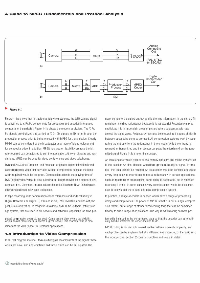
Figure 1-1a shows that in traditional television systems, the GBR camera signal
is converted to Y, Pr, Pb components for production and encoded into analog
composite for transmission. Figure 1-1b shows the modern equivalent. The Y, Pr,
Pb signals are digitized and carried as Y, Cr, Cb signals in SDI form through the
production process prior to being encoded with MPEG for transmission. Clearly,
MPEG can be considered by the broadcaster as a more efficient replacement
for composite video. In addition, MPEG has greater flexibility because the bit
rate required can be adjusted to suit the application. At lower bit rates and res-
olutions, MPEG can be used for video conferencing and video telephones.
DVB and ATSC (the European- and American-originated digital-television broad-
casting standards) would not be vi able without compression because the band-
width required would be too great. Compression extends the playing time of
DVD (digital video/versatile disc) allowing full-length movies on a standard size
compact di sc. Compressi on also reduces the cost of Electronic News Gathering and
other contributions to telev ision p roduction.
In tape recording, mild compression eases tolerances and adds reliability in
Digital Betacam and Digital-S, whereas in SX, DVC, DVCPRO, and DVCAM, the
goal is min iaturizati on. In magnetic disk drives, such as the Tektronix Profile® stor-
age system, that are used in file servers and networks (especially for news pur-
poses), compression lowers storage cost. Compression also lowers bandwidth,which allows more users to access a given server. This characteristic is also
important for VOD (Video On Demand) applications.
1.4 Introduction to Video Compression
In all real program material , there are two types of components of the signal: those
which are novel and unpredictable and those which can be anticipated. The
novel component is called entropy and is the true information in the signal. The
remainder is ca lled redundancy because it is not essential. Redundancy may be
spatial, as it is in large plain areas of picture where adjacent pixels have
almost the same value. Redundancy can also be temporal as it is where similaritie
between successive pictures are used. All compression systems work by sepa-
rating the entropy from the redundancy in the encoder. Only the entropy is
recorded or t ransmitt ed and the decoder computes the redundancy from the trans-
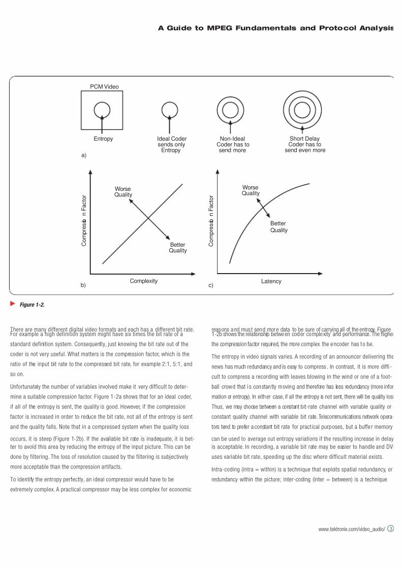
mitted signal. Figure 1-2a shows this concept.
An idea l encoder would extract all the entropy and only this wil l be t ransmit ted
to the decoder. An ideal decoder would then reproduce the original signal. In prac-
tice, this ideal cannot be reached. An ideal coder would be complex and cause
a very long delay in order to use temporal redundancy. In certain applications,
such as recording or broadcasting, some delay is acceptable, but in videocon-
ferencing it is not. In some cases, a very complex coder would be too expen-
sive. It follows that there is no one ideal compression system.
In practice, a range of coders is needed which have a range of processing
delays and complexities. The power of MPEG is that it is not a single compres-
sion format, but a range of standardized coding tools that can be combined
flexibly to suit a range of applications . The way i n which coding has been per-
formed is included in the compressed data so that the decoder can automati-cally handle whatever the coder decided to do.
MPEG coding i s div ided i nto several profiles that have different complexity, and
each profile can be implemented at a different level depending on the resolution o
the input picture. Section 2 considers profiles and levels in detail.
Figure 1-1.
AnalogComposite
Out
(PAL, NTSCor SECAM)
B
G
R
Y
PrPb
DigitalCompressed
Out
Matrix ADCProduction
ProcessB
G
R
Y
Pr
Pb
Y
Cr
Cb
Y
Cr
Cb
SDI
MPEGCoder
a)
b)
MatrixCamera
Camera
CompositeEncoder
7/16/2019 MPEG Tektronix
http://slidepdf.com/reader/full/mpeg-tektronix 9/64
There are many different digital video formats and each has a different bit rate.For example a high definition system might have six times the bit rate of a
standard definition system. Consequently, just knowing the bit rate out of the
coder is not very useful. What matters is the compression factor, which is the
ratio of the input bit rate to the compressed bit rate, for example 2:1, 5:1, and
so on.
Unfortunately the number of variables involved make it very difficult to deter-
mine a suitable compression factor. Figure 1-2a shows that for an ideal coder,
if all of the entropy is sent, the quality is good. However, if the compression
factor is increased in order to reduce the bit rate, not all of the entropy is sent
and the quality falls. Note that in a compressed system when the quality loss
occurs, it is steep (Figure 1-2b). If the available bit rate is inadequate, it is bet-
ter to avoid this area by reducing the entropy of the input picture. This can be
done by filtering. The loss of resolution caused by the filtering is subjectively
more acceptable than the compression artifacts.
To identify the entropy perfectly, an ideal compressor would have to be
extremely complex. A practical compressor may be less complex for economic
reasons and mus t send more data to be sure of carrying all of the entropy. Figure1-2b shows the relationship between coder complexity and performance. The higher
the compression factor required, the more complex the encoder has t o be.
The entropy in video signals varies. A recording of an announcer delivering the
news has much redundancy and is easy to compress . In contrast, it is more diffi -
cult to compress a recording with leaves blowing in the wind or one of a foot-
ball crowd that i s constan tly moving and therefore has less redundancy (more infor
mation or entropy). In either case, if all the entropy is not sent, there will be quality loss
Thus, we may choose between a constant bit-rate channel with variable quality or a
constant quality channel with variable bit rate. Telecommunications network opera-
tors tend to prefer a constant bit rate for pract ical purposes, but a buffe r memory
can be used to average out entropy variations if the resulting increase in delay
is acceptable. In recording, a variable bit rate may be easier to handle and DVD
uses variable bit rate, speeding up the disc where difficult material exists.
Intra-coding (intra = within) is a technique that exploits spatial redundancy, or
redundancy within the picture; inter-coding (inter = between) is a technique
A Guide to MPEG Fundamentals and Protocol Analysis
www.tektronix.com/video_audio/ 3
Figure 1-2.
Short DelayCoder has to
send even more
Non-IdealCoder has tosend more
Ideal Codersends only
Entropy
Entropy
PCM Video
WorseQuality
BetterQuality
Latency
C o m p r e s s i o
n F a c t o r
C o m p r e s s i o
n F a c t o r
WorseQuality
BetterQuality
Complexity
a)
b) c)
7/16/2019 MPEG Tektronix
http://slidepdf.com/reader/full/mpeg-tektronix 10/64
4
that exploits temporal redundancy. Intra-codi ng may be used alone, as i n the JPEG
standard for still pictures, or combined with inter-coding as in MPEG.
Intra-coding relies on two characteristics of typical images. First, not all spatial
frequencies are simultaneously present, and second, the higher the spatial fre-
quency, the lower the amplitude is likely to be. Intra-coding requires analysis of
the spatial frequencies in an image. This analysis is the purpose of transforms
such as wavelets and DCT (discrete cosine transform). Transforms produce
coefficients which describe the magnitude of each spatial frequency. Typically,
many coefficients will be zero, or nearly zero, and these coefficients can be
omit ted, resulting in a reduction in bit rate.
Inter-coding relies on finding similarities between successive pictures. If a
given pi cture i s avail able at the decoder, the next picture can be created by send-
ing only the picture differences. The picture differences will be increased when
objects move, but this magnification can be offset by using motion compensa-tion, since a moving objec t does not generally change its appearance very much
from one picture to the next. If the motion can be measured, a closer approximation
to the current picture can be created by shifting part of the previous picture to
a new location. The shifting process is controlled by a vector that is transmitted to
the decoder. The vector transmission requires less data than sending the pic-
ture-difference data.
MPEG can handle both interlaced and non-int erlaced images. An image at some
point on the time axis is called a “picture,” whether it is a fiel d or a frame.
Inte rlace is not ideal as a source for digital compression because it is in itself a com-
pression technique. Temporal coding is made more complex because pixel s in
one field are in a different position to those in the next.
Motion compensation minimizes but does not eliminate the differences between
successive pictures. The picture-di fference is it self a spatial image and can be
compressed using transform-based intra-coding as previously described.
Motion compensation simply reduces the amount of data in the difference
image.
The efficiency of a temporal coder rises with the time span over which it can act.
Figure 1-2c shows that if a high compression factor is required, a longer time
span in the input must be considered and thus a longer coding delay will be
experienced. Clearly, temporally coded signals are dif ficult to edit because the
content of a given output p icture may be based on image data which was trans-
mitted some time earlier. Production systems will have to limit the degree of
temporal coding to allow editing and this limitation will in turn limit the avail-
able compression factor.
1.5 Introduction to Audio Compression
The bit rate of a PCM digital audio channel is only about one megabit per sec-
ond, which is about 0.5% of 4:2:2 digital video. With mild video compression
schemes, such as Digital Betacam, audio compression is unnecessary. But, as
the video compression factor is raised, it becomes necessary to compress the
audio as well.
Audio compression takes advantage of two fact s. Firs t, in typi cal audio s igna ls,
not all frequencies are simultaneously present. Second, because of the phe-
nomenon of masking, human hearing cannot discern every detail of an audio
signal. Audio compression splits the audio spectrum into bands by filtering or
transforms, and includes less data when describing bands in which the level is
low. Where masking prevents or reduces audibility of a particular band, even
less data needs to be sent.
Audio compression is not as easy to achi eve as is video compressi on because
of the acuity of hearing. Masking only works properly when the masking and
the masked sounds coincide spatially. Spatial coincidence is always the case in
mono recordings but not in stereo recordings, where low-level signals can still
be heard if they are in a different part of the sound stage. Consequently, in
stereo and surround sound systems, a lower compression factor is allowable
for a given quality. Another factor complicating audio compression is that
delayed resonances in poor loudspeakers actually mask compression artifacts.
Testing a compressor with poor speakers gives a false result, and signals
which are apparently satisfactory may be disappointing when heard on good
equipment.
1.6 MPEG Signals
The output of a single MPEG audio or video coder is called an Elementary
Stream. An Elementary Stream is an endless near real-time signal. For conven
ience, it can be broken into convenient-sized data blocks in a Packetized
Elementary Stream (PES). These data blocks need header information to identi-
fy the start of the packets and must include time stamps because packetizing
disrupts the time axis.
A Guide to MPEG Fundamentals and Protocol Analysis
www.tektronix.com/video_audio/
7/16/2019 MPEG Tektronix
http://slidepdf.com/reader/full/mpeg-tektronix 11/64
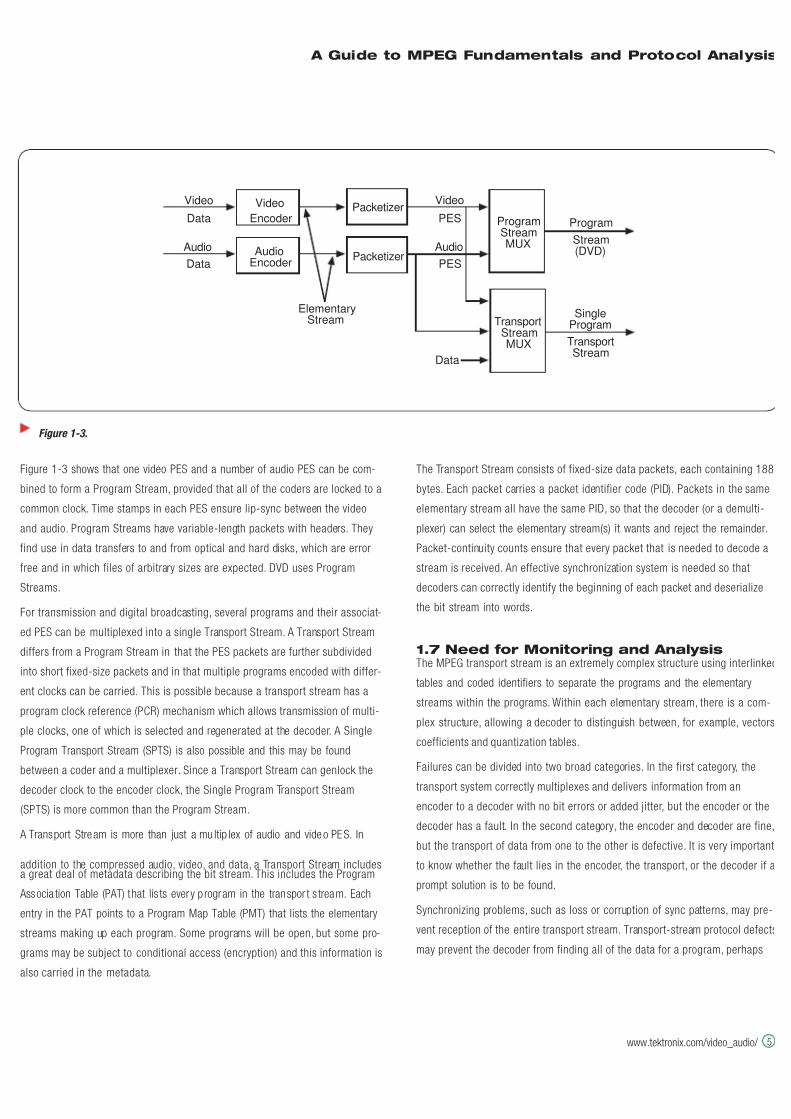
Figure 1-3 shows that one video PES and a number of audio PES can be com-
bined to form a Program Stream, provided that all of the coders are locked to a
common clock. Time stamps in each PES ensure lip-sync between the video
and audio. Program Streams have variable-length packets with headers. They
find use in data transfers to and from optical and hard disks, which are error
free and in which files of arbitrary sizes are expected. DVD uses Program
Streams.
For transmission and digital broadcasting, several programs and their associat-
ed PES can be multiplexed into a single Transport Stream. A Transport Stream
differs from a Program Stream in that the PES packets are further subdivided
into short fixed-size packets and in that multiple programs encoded with differ-
ent clocks can be carried. This is possible because a transport stream has a
program clock reference (PCR) mechanism which allows transmission of multi-
ple clocks, one of which is selected and regenerated at the decoder. A Single
Program Transport Stream (SPTS) is also possible and this may be found
between a coder and a multiplexer. Since a Transport Stream can genlock the
decoder clock to the encoder clock, the Single Program Transport Stream
(SPTS) is more common than the Program Stream.
A Transport Stream is more than just a mu ltip lex of audio and video PES. In
addition to the compressed audio, video, and data, a Transport Stream includesa great deal of metadata describing the bit stream. This includes the Program
Associa tion Table (PAT) that lis ts every p rogram in the transpor t s tream. Each
entry in the PAT points to a Program Map Table (PMT) that lists the elementary
streams making up each program. Some programs will be open, but some pro-
grams may be subject to conditional access (encryption) and this information is
also carried in the metadata.
The Transport Stream consists of fixed-size data packets, each containing 188
bytes. Each packet carries a packet identifier code (PID). Packets in the same
elementary stream all have the same PID, so that the decoder (or a demulti-
plexer) can select the elementary stream(s) it wants and reject the remainder.
Packet-continuity counts ensure that every packet that is needed to decode a
stream is received. An effective synchronization system is needed so that
decoders can correctly identify the beginning of each packet and deserialize
the bit stream into words.
1.7 Need for Monitoring and AnalysisThe MPEG transport stream is an extremely complex structure using interlinked
tables and coded identifiers to separate the programs and the elementary
streams within the programs. Within each elementary stream, there is a com-
plex structure, allowing a decoder to distinguish between, for example, vectors
coefficients and quantization tables.
Failures can be divided into two broad categories. In the first category, the
transport system correctly multiplexes and delivers information from an
encoder to a decoder with no bit errors or added jitter, but the encoder or the
decoder has a fault. In the second category, the encoder and decoder are fine,
but the transport of data from one to the other is defective. It is very important
to know whether the fault lies in the encoder, the transport, or the decoder if a
prompt solution is to be found.
Synchronizing problems, such as loss or corruption of sync patterns, may pre-
vent reception of the entire transport stream. Transport-stream protocol defects
may prevent the decoder from finding all of the data for a program, perhaps
A Guide to MPEG Fundamentals and Protocol Analysis
www.tektronix.com/video_audio/ 5
Figure 1-3.
Video
Data
Audio
Data
ElementaryStream
Video
PES
Audio
PES
Data
Program
Stream(DVD)
SingleProgram
TransportStream
Video
Encoder
AudioEncoder
Packetizer
Packetizer
ProgramStreamMUX
TransportStreamMUX
7/16/2019 MPEG Tektronix
http://slidepdf.com/reader/full/mpeg-tektronix 12/64
6
delivering picture but not sound. Correct delivery of the data but with excessive
jit ter can cause decoder timi ng probl ems.
If a system using an MPEG transport stream fails, the fault could be in the
encoder, the multiplexer, or in the decoder. How can this fault be isolated?
First, verify that a transport stream is compliant with the MPEG-coding stan-
dards. If the stream is not compliant, a decoder can hardly be blamed for hav-
ing difficulty. If it is, the decoder may need attention.
Traditional video testing tools, the signal generator, the waveform monitor, and
vectorscope, are not appropriate in analyzing MPEG systems, except to ensure
that the video signals entering and leaving an MPEG system are of suitable
quality. Instead, a reliable source of valid MPEG test signals is essential for
testing receiving equipment and decoders. With a suitable analyzer, the per-
formance of encoders, transmission systems, multiplexers, and remultiplexers
can be assessed with a high degree of confidence. As a long standing supplierof high grade test equipment to the video industry, Tektronix continues to pro-
vide test and measurement solutions as the technology evolves, giving the
MPEG user the confidence that complex compressed systems are correctly
functioning and allowing rapid diagnosis when they are not.
1.8 Pitfalls of Compression
MPEG compression is lossy in that what is decoded, is not identical to the orig-
inal. The entropy of the source varies, and when entropy is high, the compres-
sion system may leave visible artifacts when decoded. In temporal compres-
sion, redundancy between successive pictures is assumed. When this is not the
case, the system fails. An example is video from a press conference where
flashguns are firing. Individual pictures containing the flash are totally different
from their neighbors, and coding artifacts become obvious.
Irregular motion or several independently moving objects on screen require a
lot of vector bandwidth and this requirement may only be met by reducing the
picture-data bandwidth. Again, visible artifacts may occur whose level varies
and depends on the motion. This problem often occurs in sports-coverage
video.
Coarse quantizing results in luminance contouring and posterized color. These
can be seen as blotchy shadows and blocking on large areas of plain color.
Subjectively, compression artifacts are more annoying than the relatively con-
stant impairments resulting from analog television transmission systems.
The only solution to these problems is to reduce the compression factor.
Consequently, the compression user has to make a value judgment between
the economy of a high compression factor and the level of artifacts.
In addition to extending the encoding and decoding delay, temporal coding also
causes difficulty in editing. In fact, an MPEG bit stream cannot be arbitrarily
edited at all. This restriction occurs because, in temporal coding, the decoding
of one picture may require the contents of an earlier picture and the contents
may not be available following an edit. The fact that pictures may be sent out
of sequence also complicates editing.
If suitable coding has been used, edits can take place only at splice points,
which are relatively widely spaced. If arbitrary editing is required, the MPEG
stream must undergo a read-modify-write process, which will result in genera-
tion loss.
The viewer is not interested in editing, but the production user will have to
make another value judgment about the edit flexibility required. If greater flexi-
bility is required, the temporal compression has to be reduced and a higher bit
rate will be needed.
A Guide to MPEG Fundamentals and Protocol Analysis
www.tektronix.com/video_audio/
7/16/2019 MPEG Tektronix
http://slidepdf.com/reader/full/mpeg-tektronix 13/64
A Guide to MPEG Fundamentals and Protocol Analysis
www.tektronix.com/video_audio/ 7
This section shows how video compression is based on the perception of the
eye. Important enabling techniques, such as transforms and motion compensa-
tion, are considered as an introduction to the structure of an MPEG coder.
2.1 Spatial or Temporal Coding?
As was seen in Sect ion 1, video compressi on can take advantage of both spa-
tial and temporal redundancy. In MPEG, temporal redundancy is reduced first
by using similarities between successive pictures. As much as possible of the
current picture is created or “predicted” by using information from pictures
already sent. When this technique is used, it is only necessary to send a differ-
ence picture, which eliminates the differences between the actual picture and
the prediction. The difference picture is then subject to spatial compression. As
a practical matter it is easier to explain spatial compression prior to explaining
temporal compression.
Spatial compression relies on similarities between adjacent pixels in plain areas
of picture and on dominant spatial frequencies in areas of patterning. The JPEG
system uses spatial compression only, since it is designed to transmit individ-
ual still pictures. However, JPEG may be used to code a succession of individ-
ual pictures for video. In the so-called “Motion JPEG” application, the compres-
sion factor will not be as good as if temporal coding was used, but the bit
stream will be freely editable on a picture-by-picture basis.
2.2 Spatial Coding
The first step in spatial coding is to perform an analysis of spatial frequency
using a transform. A transform is simply a way of expressing a waveform in a
different domain, in this case, the frequency domain. The output of a transform
is a set of coefficients that describe how much of a given frequency is present
An inve rse transform reproduces the orig inal wave form. If the coef fici ents are
handled with sufficient accuracy, the output of the inverse transform is identica
to the original waveform.
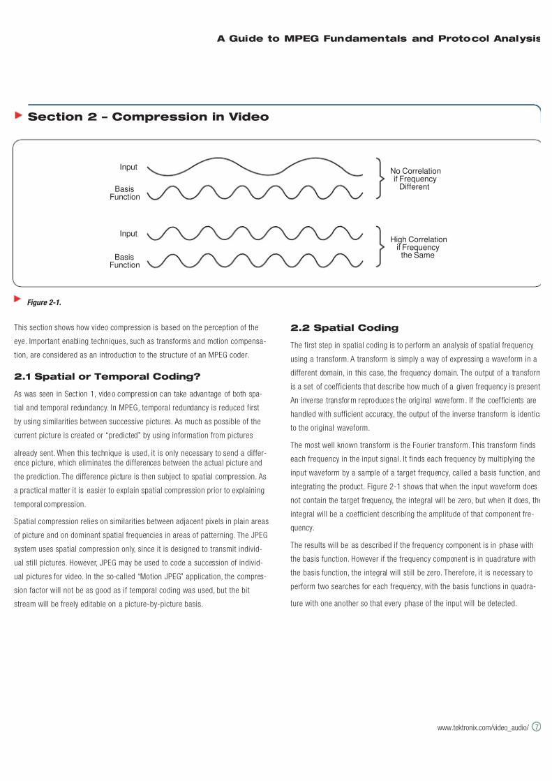
The most well known transform is the Fourier transform. This transform finds
each frequency in the input signal. It finds each frequency by multiplying the
input waveform by a sample of a target frequency, called a basis function, and
integrating the product. Figure 2-1 shows that when the input waveform does
not contain the target frequency, the integral will be zero, but when it does, the
integral will be a coefficient describing the amplitude of that component fre-
quency.
The results will be as described if the frequency component is in phase with
the basis function. However if the frequency component is in quadrature with
the basis function, the integral will still be zero. Therefore, it is necessary to
perform two searches for each frequency, with the basis functions in quadra-
ture with one another so that every phase of the input will be detected.
Section 2 – Compression in Video
Figure 2-1.
No Correlationif Frequency
Different
High Correlationif Frequencythe Same
Input
BasisFunction
Input
BasisFunction
7/16/2019 MPEG Tektronix
http://slidepdf.com/reader/full/mpeg-tektronix 14/64
8
A Guide to MPEG Fundamentals and Protocol Analysis
www.tektronix.com/video_audio/
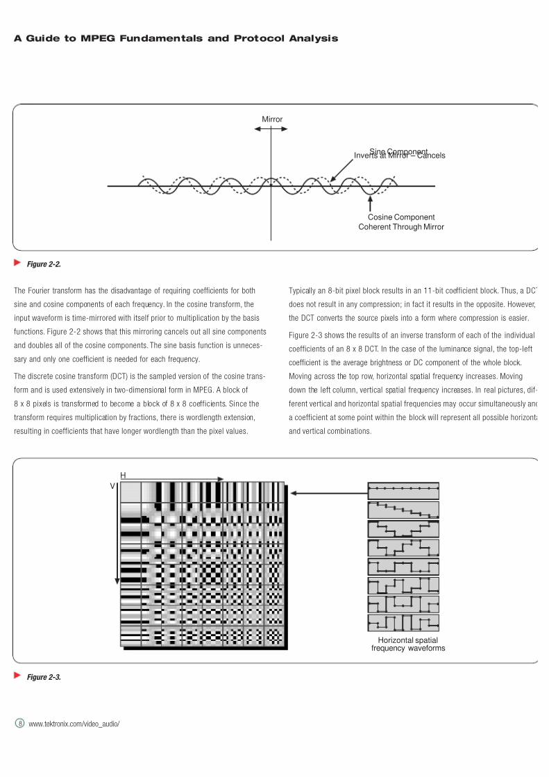
The Fourier transform has the disadvantage of requiring coefficients for both
sine and cosine components of each frequency. In the cosine transform, the
input waveform is time-mirrored with itself prior to multiplication by the basis
functions. Figure 2-2 shows that this mirroring cancels out all sine components
and doubles all of the cosine components. The sine basis function is unneces-
sary and only one coefficient is needed for each frequency.
The discrete cosine transform (DCT) is the sampled version of the cosine trans-
form and is used extensively in two-dimensional form in MPEG. A block of
8 x 8 pixels is transformed to become a block of 8 x 8 coefficients. Since the
transform requires multiplication by fractions, there is wordlength extension,
resulting in coefficients that have longer wordlength than the pixel values.
Typically an 8-bit pixel block results in an 11-bit coefficient block. Thus, a DCT
does not result in any compression; in fact it results in the opposite. However,
the DCT converts the source pixels into a form where compression is easier.
Figure 2-3 shows the results of an inverse transform of each of the individual
coefficients of an 8 x 8 DCT. In the case of the luminance signal, the top-left
coefficient is the average brightness or DC component of the whole block.
Moving across the top row, horizontal spatial frequency increases. Moving
down the left column, vertical spatial frequency increases. In real pictures, dif-
ferent vertical and horizontal spatial frequencies may occur simultaneously and
a coefficient at some point within the block will represent all possible horizonta
and vertical combinations.
Figure 2-2.
Mirror
Cosine Component
Coherent Through Mirror
Sine ComponentInverts at Mirror – Cancels
Figure 2-3.
Horizontal spatialfrequency waveforms
H
V
7/16/2019 MPEG Tektronix
http://slidepdf.com/reader/full/mpeg-tektronix 15/64
A Guide to MPEG Fundamentals and Protocol Analysis
www.tektronix.com/video_audio/ 9
Figure 2-3 also shows the coefficients as a one-dimensional horizontal wave-
form. Combining these waveforms with various amplitudes and either polarity
can reproduce any combination of 8 pixels. Thus combining the 64 coefficients
of the 2-D DCT will result in the original 8 x 8 pixel block. Clearly for color pic-
tures, the color difference samples will also need to be handled. Y, Cr, and Cb
data are assembled into separate 8 x 8 arrays and are transformed individually.
In much real program material, many of the coefficients will have zero or near-
zero values and, therefore, will not be transmitted. This fact results in signifi-
cant compression that is virtually lossless. If a higher compression factor is
needed, then the wordlength of the non-zero coefficients must be reduced. This
reduction will reduce accuracy of these coefficients and will introduce losses
into the process. With care, the losses can be introduced in a way that is least
visible to the viewer.
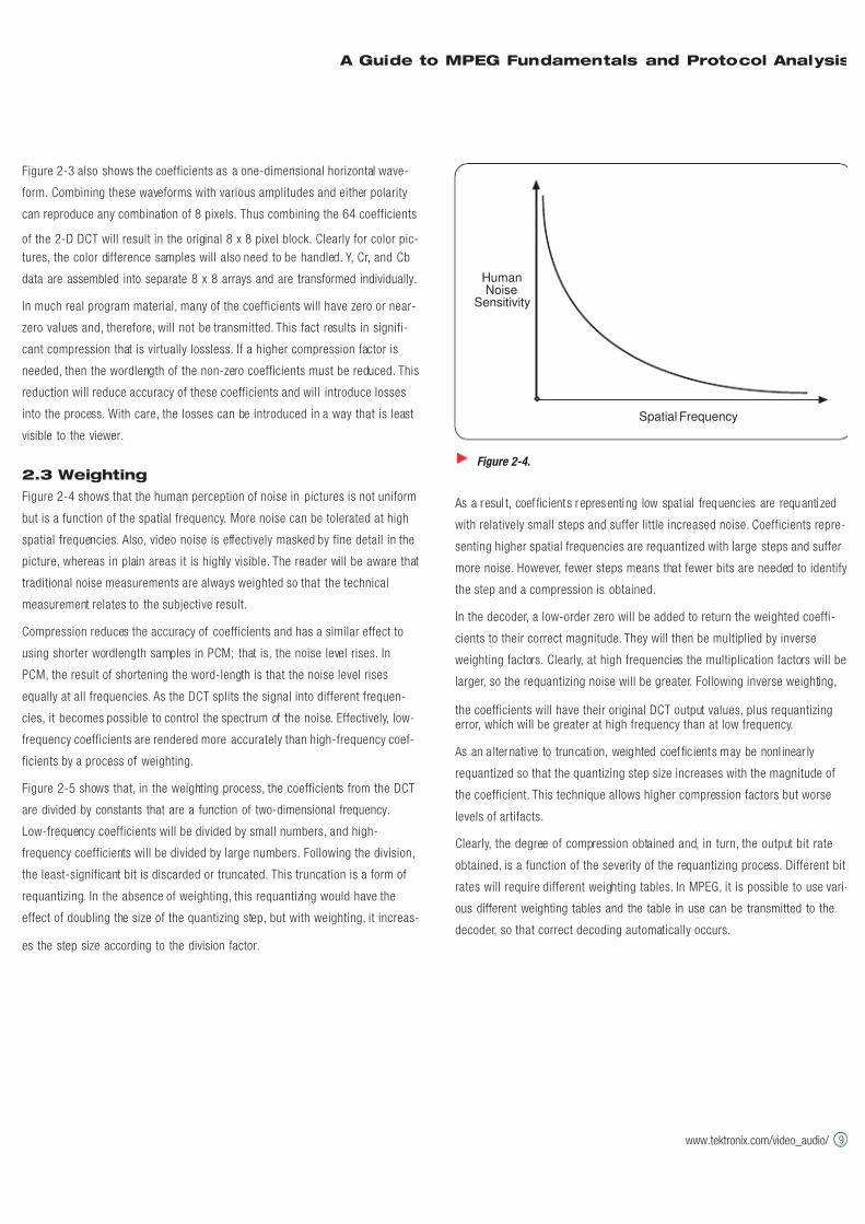
2.3 Weighting
Figure 2-4 shows that the human perception of noise in pictures is not uniform
but is a function of the spatial frequency. More noise can be tolerated at high
spatial frequencies. Also, video noise is effectively masked by fine detail in the
picture, whereas in plain areas it is highly visible. The reader will be aware that
traditional noise measurements are always weighted so that the technical
measurement relates to the subjective result.
Compression reduces the accuracy of coefficients and has a similar effect to
using shorter wordlength samples in PCM; that is, the noise level rises. In
PCM, the result of shortening the word-length is that the noise level rises
equally at all frequencies. As the DCT splits the signal into different frequen-
cies, it becomes possible to control the spectrum of the noise. Effectively, low-
frequency coefficients are rendered more accurately than high-frequency coef-
ficients by a process of weighting.
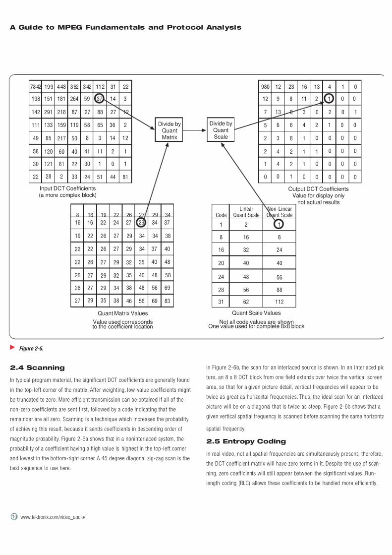
Figure 2-5 shows that, in the weighting process, the coefficients from the DCT
are divided by constants that are a function of two-dimensional frequency.
Low-frequency coefficients will be divided by small numbers, and high-
frequency coefficients will be divided by large numbers. Following the division,
the least-significant bit is discarded or truncated. This truncation is a form of
requantizing. In the absence of weighting, this requantizing would have the
effect of doubling the size of the quantizing step, but with weighting, it increas-
es the step size according to the division factor.
As a resul t, coef fic ients representing low spat ial frequencies are requanti zed
with relatively small steps and suffer little increased noise. Coefficients repre-
senting higher spatial frequencies are requantized with large steps and suffer
more noise. However, fewer steps means that fewer bits are needed to identify
the step and a compression is obtained.
In the decoder, a low-order zero will be added to return the weighted coeffi-
cients to their correct magnitude. They will then be multiplied by inverse
weighting factors. Clearly, at high frequencies the multiplication factors will be
larger, so the requantizing noise will be greater. Following inverse weighting,
the coefficients will have their original DCT output values, plus requantizingerror, which will be greater at high frequency than at low frequency.
As an a lternati ve to truncati on, weighted coef fic ients may be nonl inear ly
requantized so that the quantizing step size increases with the magnitude of
the coefficient. This technique allows higher compression factors but worse
levels of artifacts.
Clearly, the degree of compression obtained and, in turn, the output bit rate
obtained, is a function of the severity of the requantizing process. Different bit
rates will require different weighting tables. In MPEG, it is possible to use vari-
ous different weighting tables and the table in use can be transmitted to the
decoder, so that correct decoding automatically occurs.
Figure 2-4.
HumanNoise
Sensitivity
Spatial Frequency
7/16/2019 MPEG Tektronix
http://slidepdf.com/reader/full/mpeg-tektronix 16/64
10
A Guide to MPEG Fundamentals and Protocol Analysis
www.tektronix.com/video_audio/
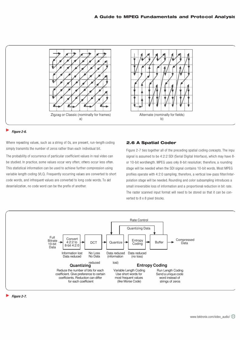
2.4 Scanning
In typical program material, the significant DCT coefficients are generally found
in the top-left corner of the matrix. After weighting, low-value coefficients might
be truncated to zero. More efficient transmission can be obtained if all of the
non-zero coefficients are sent first, followed by a code indicating that the
remainder are all zero. Scanning is a technique which increases the probability
of achieving this result, because it sends coefficients in descending order of
magnitude probability. Figure 2-6a shows that in a noninterlaced system, the
probability of a coefficient having a high value is highest in the top-left corner
and lowest in the bottom-right corner. A 45 degree diagonal zig-zag scan is the
best sequence to use here.
In Figure 2-6b, the scan for an interlaced source is shown. In an interlaced pic
ture, an 8 x 8 DCT block from one field extends over twice the vertical screen
area, so that for a given picture detail, vertical frequencies will appear to be
twice as great as horizontal frequencies. Thus, the ideal scan for an interlaced
picture will be on a diagonal that is twice as steep. Figure 2-6b shows that a
given vertical spatial frequency is scanned before scanning the same horizonta
spatial frequency.
2.5 Entropy Coding
In real video, not all spatial frequencies are simultaneously present; therefore,
the DCT coefficient matrix will have zero terms in it. Despite the use of scan-
ning, zero coefficients will still appear between the significant values. Run-
length coding (RLC) allows these coefficients to be handled more efficiently.
Figure 2-5.
Input DCT Coefficients(a more complex block)
Output DCT CoefficientsValue for display only
not actual results
Quant Matrix Values
Value used correspondsto the coefficient location
Quant Scale Values
Not all code values are shownOne value used for complete 8x8 block
Divide byQuantMatrix
Divide byQuantScale
980 12 23 16 13 4 1 0
12
7
5
2
2
1
0
9 8 11 2 1 0 0
13
6
3
4
4
0
8 3 0 2 0 1
6
8
2
2
1
4 2 1 0 0
1
1
1
0
0
0 0
0 0 0
1 0 0 0
0 0
0 00 0
7842 199 448 362 342 112 31 22
198
142
111
49
58
30
22
151 181 264 59 37 14 3
291
133
85
120
121
28
218 87 27 88 27 12
159
217
60
61
2
119 58 65 36 2
50
40
22
33
8 3 14 12
41 11 2 1
30 1 0 1
24 51 44 81
8 16 19 22 26 27 29 34
16
19
22
22
26
26
27
16 22 24 27 29 34 37
22
22
26
27
27
29
26 27 29 34 34 38
26
27
29
29
35
27 29 34 37 40
29
32
34
38
35 40 48
35 40 48
38 48 56 69
46 56 69 83
32
58
CodeLinear
Quant ScaleNon-LinearQuant Scale
1
8
16
20
24
28
31
2
16
32
40
48
56
62
1
8
24
40
88
112
56
7/16/2019 MPEG Tektronix
http://slidepdf.com/reader/full/mpeg-tektronix 17/64
A Guide to MPEG Fundamentals and Protocol Analysis
www.tektronix.com/video_audio/ 11
Where repeating values, such as a string of 0s, are present, run-length coding
simply transmits the number of zeros rather than each individual bit.
The probability of occurrence of particular coefficient values in real video can
be studied. In practice, some values occur very often; others occur less often.
This statistical information can be used to achieve further compression using
variable length coding (VLC). Frequently occurring values are converted to short
code words, and infrequent values are converted to long code words. To aid
deserialization, no code word can be the prefix of another.
2.6 A Spatial Coder
Figure 2-7 ties together all of the preceding spatial coding concepts. The input
signal is assumed to be 4:2:2 SDI (Serial Digital Interface), which may have 8-
or 10-bit wordlength. MPEG uses only 8-bit resolution; therefore, a rounding
stage will be needed when the SDI signal contains 10-bit words. Most MPEG
profiles operate with 4:2:0 sampling; therefore, a vertical low-pass filter/inter-
polation stage will be needed. Rounding and color subsampling introduces a
small irreversible loss of information and a proportional reduction in bit rate.
The raster scanned input format will need to be stored so that it can be con-
verted to 8 x 8 pixel blocks.
Figure 2-6.
Zigzag or Classic (nominally for frames)a)
Alternate (nominally for fields)b)
Figure 2-7.
Quantizing
FullBitrate10-bitData
Rate Control
Quantizing Data
CompressedData
Data reduced(no loss)
Data reduced(information
lost)
No LossNo Data
reduced
Information lostData reduced
Convert4:2:2 to
8-bit 4:2:0Quantize
EntropyCoding BufferDCT
Entropy CodingReduce the number of bits for each
coefficient. Give preference to certaincoefficients. Reduction can differ
for each coefficient
Variable Length CodingUse short words formost frequent values
(like Morse Code)
Run Length CodingSend a unique code
word instead ofstrings of zeros
7/16/2019 MPEG Tektronix
http://slidepdf.com/reader/full/mpeg-tektronix 18/64
12
A Guide to MPEG Fundamentals and Protocol Analysis
www.tektronix.com/video_audio/
The DCT stage transforms the picture information to the frequency domain. The
DCT itself does not achieve any compression. Following DCT, the coefficients
are weighted and truncated, providing the first significant compression. The
coefficients are then zig-zag scanned to increase the probability that the signif-
icant coefficients occur early in the scan. After the last non-zero coefficient, an
EOB (end of block) code is generated.
Coefficient data are further compressed by run-length and variable-length cod-
ing. In a variable bit-rate system, the quantizing is fixed, but in a fixed bit-rate
system, a buffer memory is used to absorb variations in coding difficulty. Highly
detailed pictures will tend to fill the buffer, whereas plain pictures will allow it
to empty. If the buffer is in danger of overflowing, the requantizing steps will
have to be made larger, so that the compression factor is effectively raised.
In the decoder, the bit stream is deserialized and the entropy coding is
reversed to reproduce the weighted coefficients. The inverse weighting is
applied and coefficients are placed in the matrix according to the zig-zag scan
to recreate the DCT matrix. Following an inverse transform, the 8 x 8 pixel
block is recreated. To obtain a raster-scanned output, the blocks are stored in
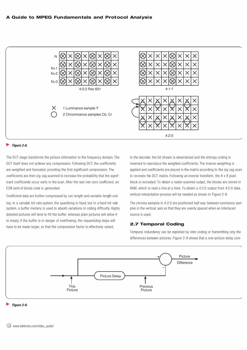
RAM, which is read a line at a time. To obtain a 4:2:2 output from 4:2:0 data,
vertical interpolation process will be needed as shown in Figure 2-8.
The chroma samples in 4:2:0 are positioned half way between luminance sam
ples in the vertical axis so that they are evenly spaced when an interlaced
source is used.
2.7 Temporal Coding
Temporal redundancy can be exploited by inter-coding or transmitting only the
differences between pictures. Figure 2-9 shows that a one-picture delay com-
Figure 2-8.
4:2:2 Rec 601 4:1:1
4:2:0
1 Luminance sample Y
2 Chrominance samples Cb, Cr
N
N+1
N+2
N+3
Figure 2-9.
ThisPicture
PreviousPicture
Picture
Difference
Picture Delay
+
_
7/16/2019 MPEG Tektronix
http://slidepdf.com/reader/full/mpeg-tektronix 19/64
A Guide to MPEG Fundamentals and Protocol Analysis
www.tektronix.com/video_audio/ 13
bined with a subtractor can compute the picture differences. The picture differ-
ence is an image in its own right and can be further compressed by the spatial
coder as was previously described. The decoder reverses the spatial coding
and adds the difference picture to the previous picture to obtain the next
picture.
There are some disadvantages to this simple system. First, as only differences
are sent, it is impossible to begin decoding after the start of the transmission.
This limitation makes it difficult for a decoder to provide pictures following a
switch from one bit stream to another (as occurs when the viewer changes
channels). Second, if any part of the difference data is incorrect, the error in
the picture will propagate indefinitely.
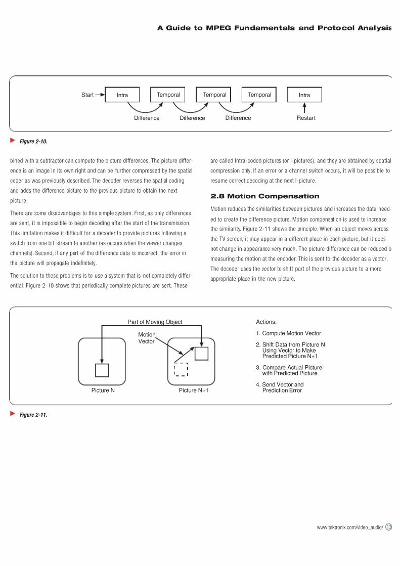
The solution to these problems is to use a system that is not completely differ-
ential. Figure 2-10 shows that periodically complete pictures are sent. These
are called Intra-coded pictures (or I-pictures), and they are obtained by spatial
compression only. If an error or a channel switch occurs, it will be possible to
resume correct decoding at the next I-picture.
2.8 Motion Compensation
Motion reduces the similarities between pictures and increases the data need-
ed to create the difference picture. Motion compensation is used to increase
the similarity. Figure 2-11 shows the principle. When an object moves across
the TV screen, it may appear in a different place in each picture, but it does
not change in appearance very much. The picture difference can be reduced by
measuring the motion at the encoder. This is sent to the decoder as a vector.
The decoder uses the vector to shift part of the previous picture to a more
appropriate place in the new picture.
Figure 2-10.
Difference Restart
Start Intra IntraTemporal Temporal Temporal
DifferenceDifference
Figure 2-11.
Actions:
1. Compute Motion Vector
2. Shift Data from Picture NUsing Vector to MakePredicted Picture N+1
3. Compare Actual Picturewith Predicted Picture
4. Send Vector andPrediction ErrorPicture N Picture N+1
MotionVector
Part of Moving Object
7/16/2019 MPEG Tektronix
http://slidepdf.com/reader/full/mpeg-tektronix 20/64
14
A Guide to MPEG Fundamentals and Protocol Analysis
www.tektronix.com/video_audio/
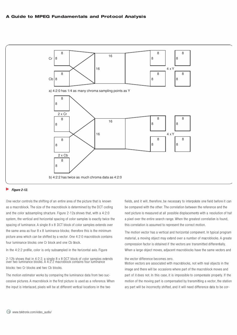
One vector controls the shifting of an entire area of the picture that is known
as a macroblock. The size of the macroblock is determined by the DCT coding
and the color subsampling structure. Figure 2-12a shows that, with a 4:2:0
system, the vertical and horizontal spacing of color samples is exactly twice the
spacing of luminance. A single 8 x 8 DCT block of color samples extends over
the same area as four 8 x 8 luminance blocks; therefore this is the minimum
picture area which can be shifted by a vector. One 4:2:0 macroblock contains
four luminance blocks: one Cr block and one Cb block.
In the 4:2:2 profile, color is only subsampled in the horizontal axis. Figure
2-12b shows that in 4:2:2, a single 8 x 8 DCT block of color samples extendsover two luminance blocks. A 4:2:2 macroblock contains four luminance
blocks: two Cr blocks and two Cb blocks.
The motion estimator works by comparing the luminance data from two suc-
cessive pictures. A macroblock in the first picture is used as a reference. When
the input is interlaced, pixels will be at different vertical locations in the two
fields, and it will, therefore, be necessary to interpolate one field before it can
be compared with the other. The correlation between the reference and the
next picture is measured at all possible displacements with a resolution of half
a pixel over the entire search range. When the greatest correlation is found,
this correlation is assumed to represent the correct motion.
The motion vector has a vertical and horizontal component. In typical program
material, a moving object may extend over a number of macroblocks. A greater
compression factor is obtained if the vectors are transmitted differentially.
When a large object moves, adjacent macroblocks have the same vectors and
the vector difference becomes zero.
Motion vectors are associated with macroblocks, not with real objects in the
image and there will be occasions where part of the macroblock moves and
part of it does not. In this case, it is impossible to compensate properly. If the
motion of the moving part is compensated by transmitting a vector, the station-
ary part will be incorrectly shifted, and it will need difference data to be cor-
Figure 2-12.
a) 4:2:0 has 1/4 as many chroma sampling points as Y
b) 4:2:2 has twice as much chroma data as 4:2:0
8
8
8
8
8
8
8
8
8
8
8
8
16
16 4 x Y
Cr
Cb
8
8
8
8
2 x Cr
2 x Cb
16
16
8
8
8
8
8
8
8
8
4 x Y
8
8
8
8
7/16/2019 MPEG Tektronix
http://slidepdf.com/reader/full/mpeg-tektronix 21/64
A Guide to MPEG Fundamentals and Protocol Analysis
www.tektronix.com/video_audio/ 15
rected. If no vector is sent, the stationary part will be correct, but difference
data will be needed to correct the moving part. A practical compressor might
attempt both strategies and select the one which required the least difference
data.
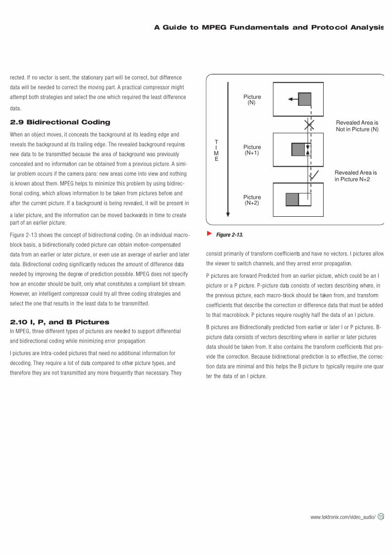
2.9 Bidirectional Coding
When an object moves, it conceals the background at its leading edge and
reveals the background at its trailing edge. The revealed background requires
new data to be transmitted because the area of background was previously
concealed and no information can be obtained from a previous picture. A simi-
lar problem occurs if the camera pans: new areas come into view and nothing
is known about them. MPEG helps to minimize this problem by using bidirec-
tional coding, which allows information to be taken from pictures before and
after the current picture. If a background is being revealed, it will be present in
a later picture, and the information can be moved backwards in time to create
part of an earlier picture.
Figure 2-13 shows the concept of bidirectional coding. On an individual macro-
block basis, a bidirectionally coded picture can obtain motion-compensated
data from an earlier or later picture, or even use an average of earlier and later
data. Bidirectional coding significantly reduces the amount of difference data
needed by improving the degree of prediction possible. MPEG does not specify
how an encoder should be built, only what constitutes a compliant bit stream.
However, an intelligent compressor could try all three coding strategies and
select the one that results in the least data to be transmitted.
2.10 I, P, and B Pictures
In MPEG, three different types of pictures are needed to support differential
and bidirectional coding while minimizing error propagation:
I pictures are Intra-coded pictures that need no additional information for
decoding. They require a lot of data compared to other picture types, and
therefore they are not transmitted any more frequently than necessary. They
consist primarily of transform coefficients and have no vectors. I pictures allow
the viewer to switch channels, and they arrest error propagation.
P pictures are forward Predicted from an earlier picture, which could be an I
picture or a P picture. P-picture data consists of vectors describing where, in
the previous picture, each macro-block should be taken from, and transform
coefficients that describe the correction or difference data that must be added
to that macroblock. P pictures require roughly half the data of an I picture.
B pictures are Bidirectionally predicted from earlier or later I or P pictures. B-
picture data consists of vectors describing where in earlier or later pictures
data should be taken from. It also contains the transform coefficients that pro-
vide the correction. Because bidirectional prediction is so effective, the correc-
tion data are minimal and this helps the B picture to typically require one quar
ter the data of an I picture.
Figure 2-13.
Revealed Area isNot in Picture (N)
Revealed Area isin Picture N+2
Picture(N)
Picture(N+1)
Picture(N+2)
TIME
7/16/2019 MPEG Tektronix
http://slidepdf.com/reader/full/mpeg-tektronix 22/64
16
A Guide to MPEG Fundamentals and Protocol Analysis
www.tektronix.com/video_audio/
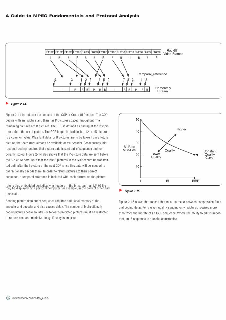
Figure 2-14 introduces the concept of the GOP or Group Of Pictures. The GOP
begins with an I picture and then has P pictures spaced throughout. The
remaining pictures are B pictures. The GOP is defined as ending at the last pic-
ture before the next I picture. The GOP length is flexible, but 12 or 15 pictures
is a common value. Clearly, if data for B pictures are to be taken from a future
picture, that data must already be available at the decoder. Consequently, bidi-
rectional coding requires that picture data is sent out of sequence and tem-
porarily stored. Figure 2-14 also shows that the P-picture data are sent before
the B-picture data. Note that the last B pictures in the GOP cannot be transmit-
ted until after the I picture of the next GOP since this data will be needed to
bidirectionally decode them. In order to return pictures to their correct
sequence, a temporal reference is included with each picture. As the picture
rate is also embedded periodically in headers in the bit stream, an MPEG filemay be displayed by a personal computer, for example, in the correct order and
timescale.
Sending picture data out of sequence requires additional memory at the
encoder and decoder and also causes delay. The number of bidirectionally
coded pictures between intra- or forward-predicted pictures must be restricted
to reduce cost and minimize delay, if delay is an issue.
Figure 2-15 shows the tradeoff that must be made between compression factor
and coding delay. For a given quality, sending only I pictures requires more
than twice the bit rate of an IBBP sequence. Where the ability to edit is impor-
tant, an IB sequence is a useful compromise.
Figure 2-15.
Bit RateMBit/Sec
LowerQuality
Higher
Quality ConstantQualityCurve
10 –
20 –
30 –
40 –
50 –
I IB IBBP
Figure 2-14.
Rec 601Video Frames
ElementaryStream
temporal_reference
I B PB B PB B B I B PB
Frame Frame Frame FrameFrame Frame Frame Frame Frame Frame Frame Frame Frame
I IB B B B B BB BP P P
0 3 1 2 6 4 5 0 7 8 3 1 2
7/16/2019 MPEG Tektronix
http://slidepdf.com/reader/full/mpeg-tektronix 23/64
A Guide to MPEG Fundamentals and Protocol Analysis
www.tektronix.com/video_audio/ 17
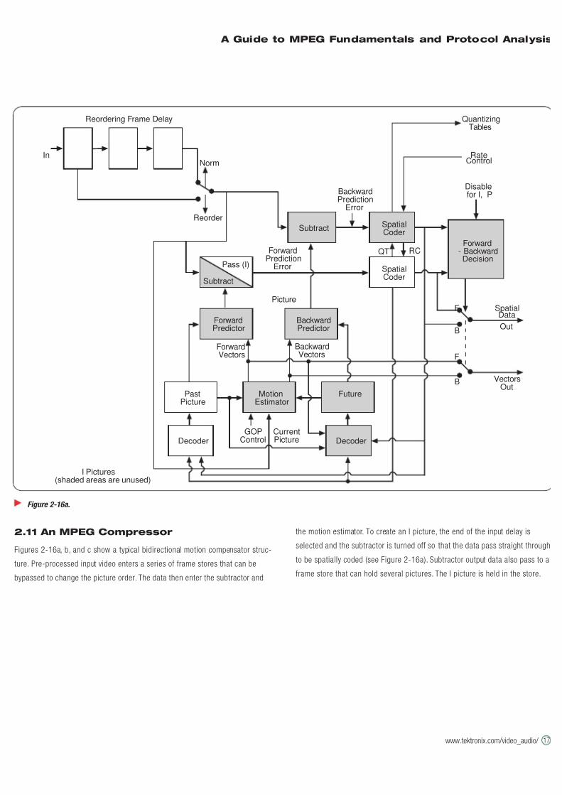
2.11 An MPEG Compressor
Figures 2-16a, b, and c show a typical bidirectional motion compensator struc-
ture. Pre-processed input video enters a series of frame stores that can be
bypassed to change the picture order. The data then enter the subtractor and
the motion estimator. To create an I picture, the end of the input delay is
selected and the subtractor is turned off so that the data pass straight through
to be spatially coded (see Figure 2-16a). Subtractor output data also pass to a
frame store that can hold several pictures. The I picture is held in the store.
Figure 2-16a.
Reordering Frame Delay QuantizingTables
In
SpatialCoder
RateControl
BackwardPrediction
Error
Disablefor I, P
SpatialData
VectorsOut
ForwardPrediction
Error
Norm
Reorder
ForwardVectors
BackwardVectors
GOPControl
CurrentPicture
Out
F
B
F
B
QT RC
Subtract SpatialCoder
Forward
- Backward
Decision
ForwardPredictor
BackwardPredictor
MotionEstimator
Future
Picture
DecoderDecoder
Subtract
Pass (I)
I Pictures(shaded areas are unused)
PastPicture
7/16/2019 MPEG Tektronix
http://slidepdf.com/reader/full/mpeg-tektronix 24/64
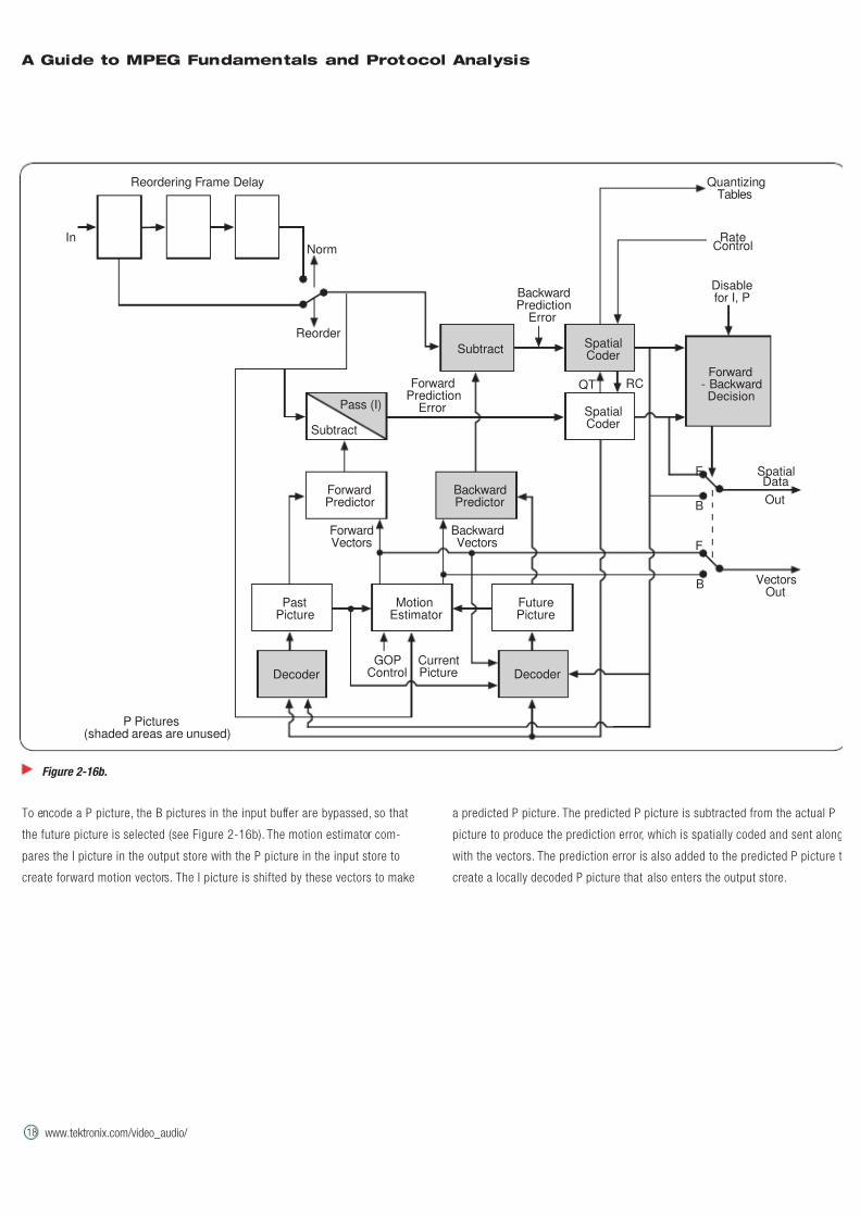
To encode a P picture, the B pictures in the input buffer are bypassed, so that
the future picture is selected (see Figure 2-16b). The motion estimator com-
pares the I picture in the output store with the P picture in the input store to
create forward motion vectors. The I picture is shifted by these vectors to make
a predicted P picture. The predicted P picture is subtracted from the actual P
picture to produce the prediction error, which is spatially coded and sent along
with the vectors. The prediction error is also added to the predicted P picture t
create a locally decoded P picture that also enters the output store.
18
A Guide to MPEG Fundamentals and Protocol Analysis
www.tektronix.com/video_audio/
Figure 2-16b.
Reordering Frame Delay QuantizingTables
In
SpatialCoder
RateControl
BackwardPrediction
Error
Disablefor I, P
SpatialData
VectorsOut
ForwardPrediction
Error
Norm
Reorder
ForwardVectors
BackwardVectors
GOPControl
CurrentPicture
Out
F
B
F
QT RC
Subtract SpatialCoder
Forward
- Backward
Decision
BackwardPredictor
FuturePicture
Decoder
P Pictures(shaded areas are unused)
ForwardPredictor
MotionEstimator
PastPicture
Subtract
Pass (I)
Decoder
B
7/16/2019 MPEG Tektronix
http://slidepdf.com/reader/full/mpeg-tektronix 25/64
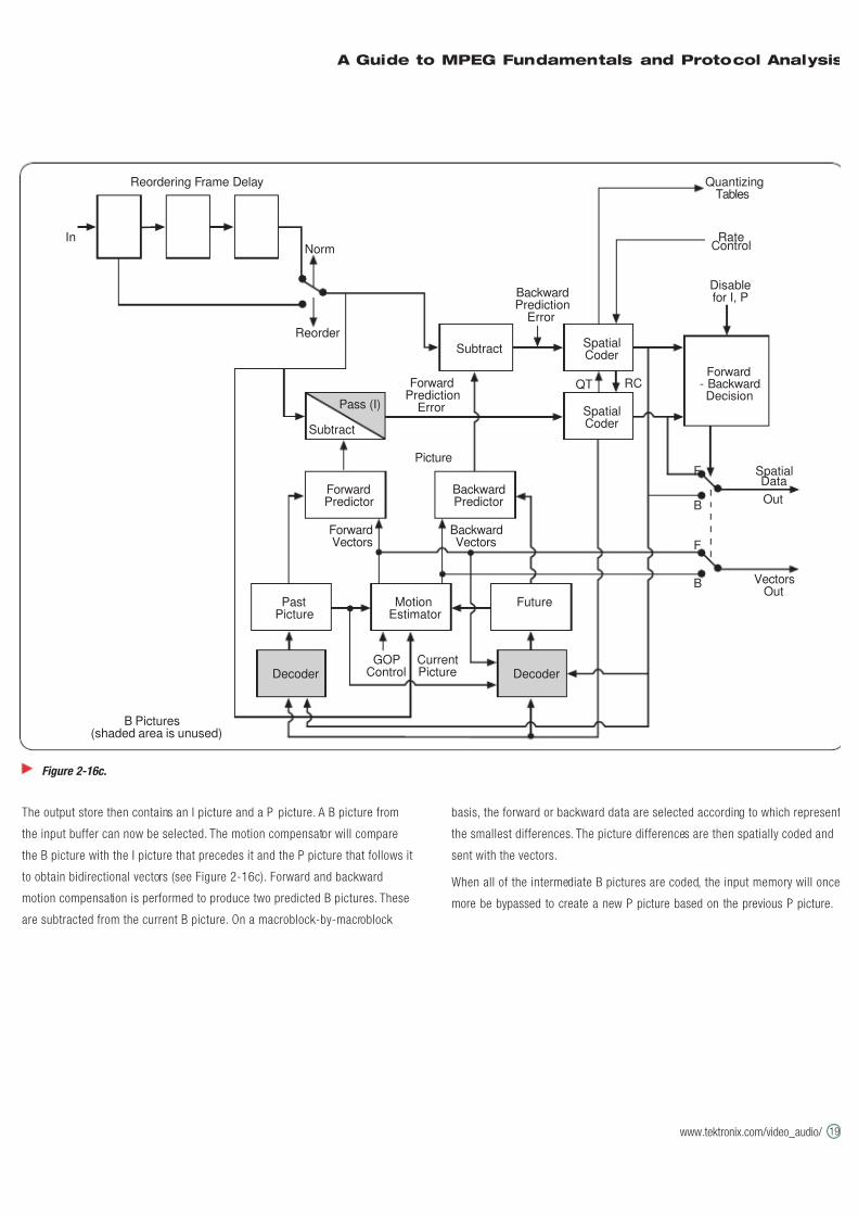
The output store then contains an I picture and a P picture. A B picture from
the input buffer can now be selected. The motion compensator will compare
the B picture with the I picture that precedes it and the P picture that follows it
to obtain bidirectional vectors (see Figure 2-16c). Forward and backward
motion compensation is performed to produce two predicted B pictures. These
are subtracted from the current B picture. On a macroblock-by-macroblock
basis, the forward or backward data are selected according to which represent
the smallest differences. The picture differences are then spatially coded and
sent with the vectors.
When all of the intermediate B pictures are coded, the input memory will once
more be bypassed to create a new P picture based on the previous P picture.
A Guide to MPEG Fundamentals and Protocol Analysis
www.tektronix.com/video_audio/ 19
Figure 2-16c.
Reordering Frame Delay QuantizingTables
In
SpatialCoder
RateControl
BackwardPrediction
Error
Disablefor I, P
SpatialData
VectorsOut
ForwardPrediction
Error
Norm
Reorder
ForwardVectors
BackwardVectors
GOPControl
CurrentPicture
Out
F
B
F
B
QT RC
ForwardPredictor
MotionEstimator
PastPicture
Decoder
Subtract
Pass (I)
Subtract SpatialCoder
Forward
- Backward
Decision
BackwardPredictor
Future
Picture
Decoder
B Pictures(shaded area is unused)
7/16/2019 MPEG Tektronix
http://slidepdf.com/reader/full/mpeg-tektronix 26/64
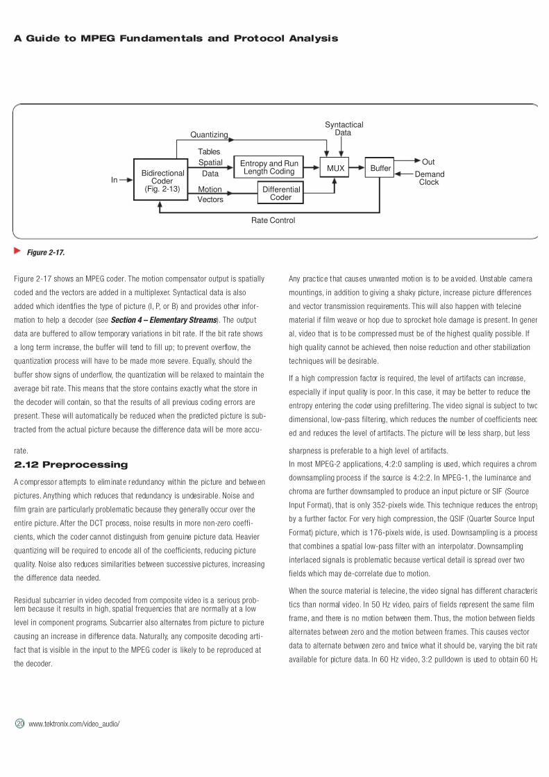
Figure 2-17 shows an MPEG coder. The motion compensator output is spatially
coded and the vectors are added in a multiplexer. Syntactical data is also
added which identifies the type of picture (I, P, or B) and provides other infor-
mation to help a decoder (see Section 4 – Elementary Streams ). The outpu t
data are buffered to allow temporary variations in bit rate. If the bit rate shows
a long term increase, the buffer will tend to fill up; to prevent overflow, the
quantization process will have to be made more severe. Equally, should the
buffer show signs of underflow, the quantization will be relaxed to maintain the
average bit rate. This means that the store contains exactly what the store in
the decoder will contain, so that the results of all previous coding errors are
present. These will automatically be reduced when the predicted picture is sub-
tracted from the actual picture because the difference data will be more accu-
rate.
2.12 Preprocessing
A compressor a ttempts to eliminate redundancy within the pic ture and between
pictures. Anything which reduces that redundancy is undesirable. Noise and
film grain are particularly problematic because they generally occur over the
entire picture. After the DCT process, noise results in more non-zero coeffi-
cients, which the coder cannot distinguish from genuine picture data. Heavier
quantizing will be required to encode all of the coefficients, reducing picture
quality. Noise also reduces similarities between successive pictures, increasing
the difference data needed.
Residual subcarrier in video decoded from composite video is a serious prob-lem because it results in high, spatial frequencies that are normally at a low
level in component programs. Subcarrier also alternates from picture to picture
causing an increase in difference data. Naturally, any composite decoding arti-
fact that is visible in the input to the MPEG coder is likely to be reproduced at
the decoder.
Any practice that causes unwanted motion is to be avoided. Unstable camera
mountings, in addition to giving a shaky picture, increase picture differences
and vector transmission requirements. This will also happen with telecine
material if film weave or hop due to sprocket hole damage is present. In gener
al, video that is to be compressed must be of the highest quality possible. If
high quality cannot be achieved, then noise reduction and other stabilization
techniques will be desirable.
If a high compression factor is required, the level of artifacts can increase,
especially if input quality is poor. In this case, it may be better to reduce the
entropy entering the coder using prefiltering. The video signal is subject to two
dimensional, low-pass filtering, which reduces the number of coefficients need
ed and reduces the level of artifacts. The picture will be less sharp, but less
sharpness is preferable to a high level of artifacts.
In most MPEG-2 applications, 4:2:0 sampling is used, which requires a chroma
downsampling process if the source is 4:2:2. In MPEG-1, the luminance and
chroma are further downsampled to produce an input picture or SIF (Source
Input Format), that is only 352-pixels wide. This technique reduces the entropy
by a further factor. For very high compression, the QSIF (Quarter Source Input
Format) picture, which is 176-pixels wide, is used. Downsampling is a process
that combines a spatial low-pass filter with an interpolator. Downsampling
interlaced signals is problematic because vertical detail is spread over two
fields which may de-correlate due to motion.
When the source material is telecine, the video signal has different characteris
tics than normal video. In 50 Hz video, pairs of fields represent the same film
frame, and there is no motion between them. Thus, the motion between fields
alternates between zero and the motion between frames. This causes vector
data to alternate between zero and twice what it should be, varying the bit rate
available for picture data. In 60 Hz video, 3:2 pulldown is used to obtain 60 Hz
20
A Guide to MPEG Fundamentals and Protocol Analysis
www.tektronix.com/video_audio/
Figure 2-17.
In
Out
DemandClock
MUX Buffer
Quantizing
Tables
Spatial
Data
Motion
Vectors
SyntacticalData
Rate Control
Entropy and RunLength Coding
DifferentialCoder
BidirectionalCoder
(Fig. 2-13)
7/16/2019 MPEG Tektronix
http://slidepdf.com/reader/full/mpeg-tektronix 27/64
A Guide to MPEG Fundamentals and Protocol Analysis
www.tektronix.com/video_audio/ 21
from 24 Hz film. One frame is made into two fields, the next is made into three
fields, and so on.
Consequently, one field in five is completely redundant. MPEG handles film
material best by discarding the third field in 3:2 systems. A 24 Hz code in the
transmission alerts the decoder to recreate the 3:2 sequence by re-reading a
field store. In 50 and 60 Hz telecine, pairs of fields are deinterlaced to create
frames, and then motion is measured between frames. The decoder can recre-
ate interlace by reading alternate lines in the frame store.
A cut is a di ffi cult event for a compressor to handle because i t r esul ts in an
almost complete prediction failure, requiring a large amount of correction data.
If a coding delay can be tolerated, a coder may detect cuts in advance and
modify the GOP structure dynamically, so that the cut is made to coincide with
the generation of an I picture. In this case, the cut is handled with very little
extra data. The last B pictures before the I frame will almost certainly need to
use forward prediction. In some applications that are not real-time, such as
DVD mastering, a coder could take two passes at the input video: one pass to
identify the difficult or high entropy areas and create a coding strategy, and a
second pass to actually compress the input video.
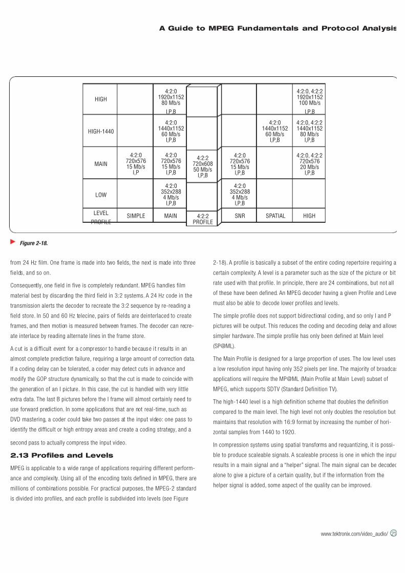
2.13 Profiles and Levels
MPEG is applicable to a wide range of applications requiring different perform-
ance and complexity. Using all of the encoding tools defined in MPEG, there are
millions of combinations possible. For practical purposes, the MPEG-2 standard
is divided into profiles, and each profile is subdivided into levels (see Figure
2-18). A profile is basically a subset of the entire coding repertoire requiring a
certain complexity. A level is a parameter such as the size of the picture or bit
rate used with that profile. In principle, there are 24 combinations, but not all
of these have been defined. An MPEG decoder having a given Profile and Leve
must also be able to decode lower profiles and levels.
The simple profile does not support bidirectional coding, and so only I and P
pictures will be output. This reduces the coding and decoding delay and allows
simpler hardware. The simple profile has only been defined at Main level
(SP@ML).
The Main Profile is designed for a large proportion of uses. The low level uses
a low resolution input having only 352 pixels per line. The majority of broadcas
applications will require the MP@ML (Main Profile at Main Level) subset of
MPEG, which supports SDTV (Standard Definition TV).
The high-1440 level is a high definition scheme that doubles the definition
compared to the main level. The high level not only doubles the resolution but
maintains that resolution with 16:9 format by increasing the number of hori-
zontal samples from 1440 to 1920.
In compression systems using spatial transforms and requantizing, it is possi-
ble to produce scaleable signals. A scaleable process is one in which the input
results in a main signal and a “helper” signal. The main signal can be decoded
alone to give a picture of a certain quality, but if the information from the
helper signal is added, some aspect of the quality can be improved.
Figure 2-18.
HIGH
HIGH-1440
MAIN
LOW
LEVEL
PROFILE
4:2:01920x1152
80 Mb/s
I,P,B
4:2:01440x1152
60 Mb/sI,P,B
4:2:0720x57615 Mb/s
I,P,B
4:2:0352x2884 Mb/sI,P,B
4:2:0720x57615 Mb/s
I,P
SIMPLE MAIN
4:2:2720x60850 Mb/s
I,P,B
4:2:2PROFILE
4:2:0352x2884 Mb/sI,P,B
4:2:0720x57615 Mb/s
I,P,B
4:2:01440x1152
60 Mb/sI,P,B
4:2:0, 4:2:21440x1152
80 Mb/sI,P,B
4:2:0, 4:2:2720x57620 Mb/s
I,P,B
4:2:0, 4:2:21920x1152100 Mb/s
I,P,B
SNR SPATIAL HIGH
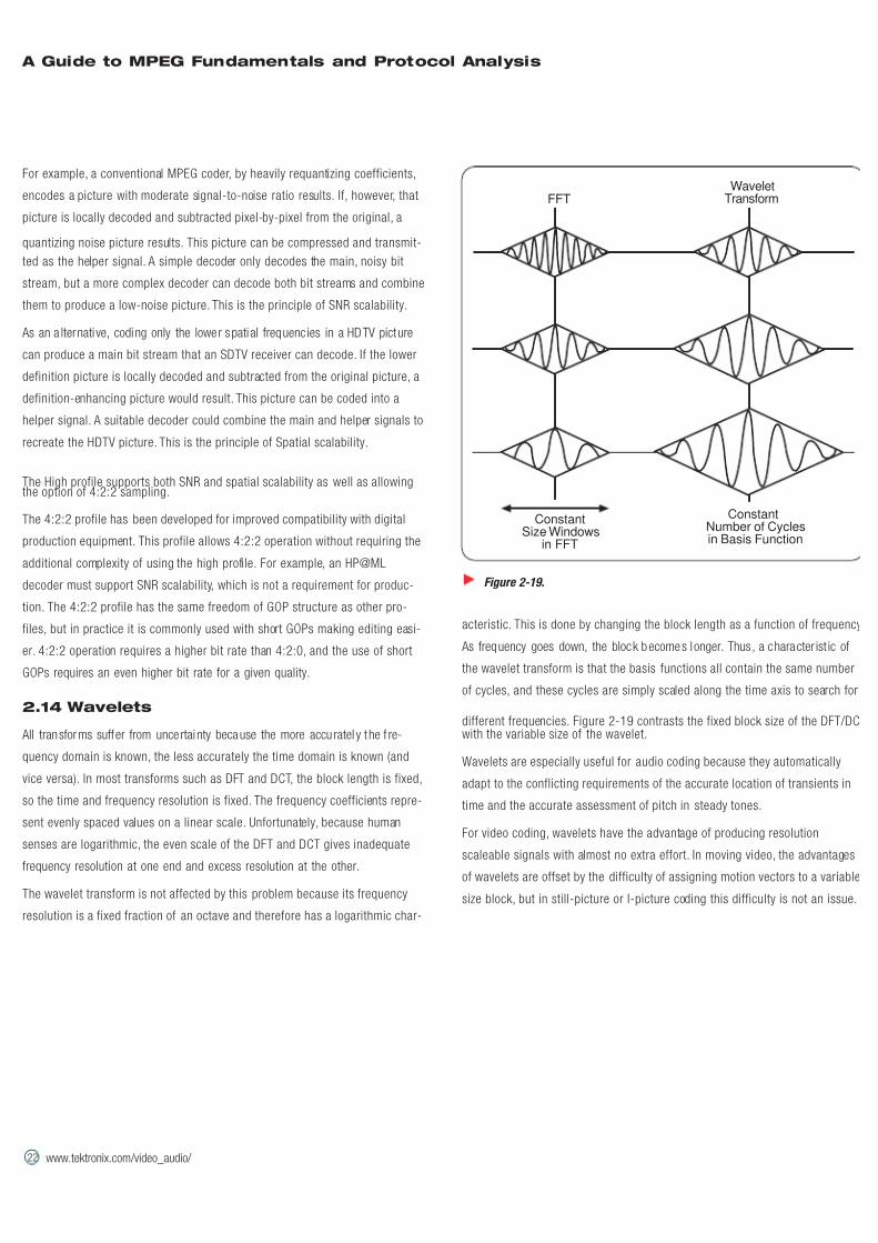
7/16/2019 MPEG Tektronix
http://slidepdf.com/reader/full/mpeg-tektronix 28/64
22
A Guide to MPEG Fundamentals and Protocol Analysis
www.tektronix.com/video_audio/
For example, a conventional MPEG coder, by heavily requantizing coefficients,
encodes a picture with moderate signal-to-noise ratio results. If, however, that
picture is locally decoded and subtracted pixel-by-pixel from the original, a
quantizing noise picture results. This picture can be compressed and transmit-
ted as the helper signal. A simple decoder only decodes the main, noisy bit
stream, but a more complex decoder can decode both bit streams and combine
them to produce a low-noise picture. This is the principle of SNR scalability.
As an a lternati ve, coding only the lower spati al frequencies in a HDTV picture
can produce a main bit stream that an SDTV receiver can decode. If the lower
definition picture is locally decoded and subtracted from the original picture, a
definition-enhancing picture would result. This picture can be coded into a
helper signal. A suitable decoder could combine the main and helper signals to
recreate the HDTV picture. This is the principle of Spatial scalability.
The High profile supports both SNR and spatial scalability as well as allowingthe option of 4:2:2 sampling.
The 4:2:2 profile has been developed for improved compatibility with digital
production equipment. This profile allows 4:2:2 operation without requiring the
additional complexity of using the high profile. For example, an HP@ML
decoder must support SNR scalability, which is not a requirement for produc-
tion. The 4:2:2 profile has the same freedom of GOP structure as other pro-
files, but in practice it is commonly used with short GOPs making editing easi-
er. 4:2:2 operation requires a higher bit rate than 4:2:0, and the use of short
GOPs requires an even higher bit rate for a given quality.
2.14 Wavelets
All transforms suffer from uncertainty because the more accu ratel y t he f re-
quency domain is known, the less accurately the time domain is known (and
vice versa). In most transforms such as DFT and DCT, the block length is fixed,
so the time and frequency resolution is fixed. The frequency coefficients repre-
sent evenly spaced values on a linear scale. Unfortunately, because human
senses are logarithmic, the even scale of the DFT and DCT gives inadequate
frequency resolution at one end and excess resolution at the other.
The wavelet transform is not affected by this problem because its frequency
resolution is a fixed fraction of an octave and therefore has a logarithmic char-
acteristic. This is done by changing the block length as a function of frequency
As frequency goes down, the block becomes l onger. Thus, a character ist ic of
the wavelet transform is that the basis functions all contain the same number
of cycles, and these cycles are simply scaled along the time axis to search for
different frequencies. Figure 2-19 contrasts the fixed block size of the DFT/DCwith the variable size of the wavelet.
Wavelets are especially useful for audio coding because they automatically
adapt to the conflicting requirements of the accurate location of transients in
time and the accurate assessment of pitch in steady tones.
For video coding, wavelets have the advantage of producing resolution
scaleable signals with almost no extra effort. In moving video, the advantages
of wavelets are offset by the difficulty of assigning motion vectors to a variable
size block, but in still-picture or I-picture coding this difficulty is not an issue.
Figure 2-19.
FFTWavelet
Transform
ConstantSize Windows
in FFT
ConstantNumber of Cyclesin Basis Function
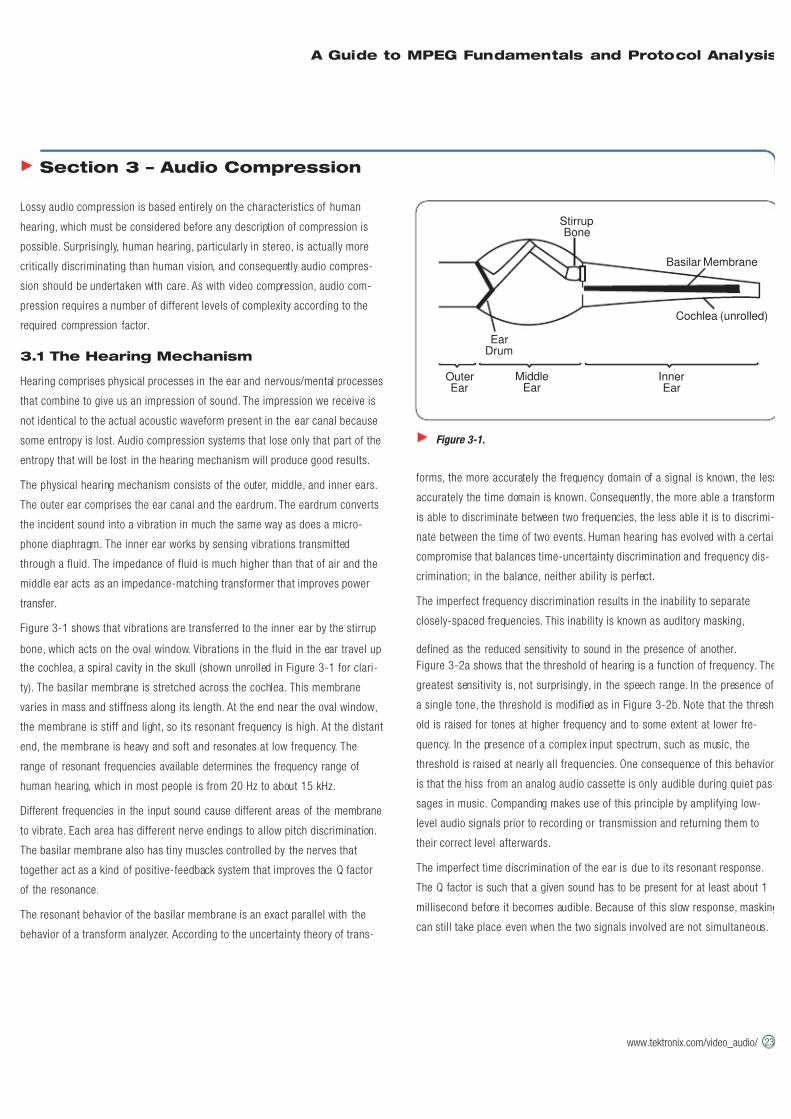
7/16/2019 MPEG Tektronix
http://slidepdf.com/reader/full/mpeg-tektronix 29/64
A Guide to MPEG Fundamentals and Protocol Analysis
www.tektronix.com/video_audio/ 23
Lossy audio compression is based entirely on the characteristics of human
hearing, which must be considered before any description of compression is
possible. Surprisingly, human hearing, particularly in stereo, is actually more
critically discriminating than human vision, and consequently audio compres-
sion should be undertaken with care. As with video compression, audio com-
pression requires a number of different levels of complexity according to the
required compression factor.
3.1 The Hearing Mechanism
Hearing comprises physical processes in the ear and nervous/mental processes
that combine to give us an impression of sound. The impression we receive is
not identical to the actual acoustic waveform present in the ear canal because
some entropy is lost. Audio compression systems that lose only that part of the
entropy that will be lost in the hearing mechanism will produce good results.
The physical hearing mechanism consists of the outer, middle, and inner ears.
The outer ear comprises the ear canal and the eardrum. The eardrum converts
the incident sound into a vibration in much the same way as does a micro-
phone diaphragm. The inner ear works by sensing vibrations transmitted
through a fluid. The impedance of fluid is much higher than that of air and the
middle ear acts as an impedance-matching transformer that improves power
transfer.
Figure 3-1 shows that vibrations are transferred to the inner ear by the stirrup
bone, which acts on the oval window. Vibrations in the fluid in the ear travel up
the cochlea, a spiral cavity in the skull (shown unrolled in Figure 3-1 for clari-
ty). The basilar membrane is stretched across the cochlea. This membrane
varies in mass and stiffness along its length. At the end near the oval window,
the membrane is stiff and light, so its resonant frequency is high. At the distant
end, the membrane is heavy and soft and resonates at low frequency. The
range of resonant frequencies available determines the frequency range of
human hearing, which in most people is from 20 Hz to about 15 kHz.
Different frequencies in the input sound cause different areas of the membrane
to vibrate. Each area has different nerve endings to allow pitch discrimination.
The basilar membrane also has tiny muscles controlled by the nerves that
together act as a kind of positive-feedback system that improves the Q factor
of the resonance.
The resonant behavior of the basilar membrane is an exact parallel with the
behavior of a transform analyzer. According to the uncertainty theory of trans-
forms, the more accurately the frequency domain of a signal is known, the less
accurately the time domain is known. Consequently, the more able a transform
is able to discriminate between two frequencies, the less able it is to discrimi-
nate between the time of two events. Human hearing has evolved with a certain
compromise that balances time-uncertainty discrimination and frequency dis-
crimination; in the balance, neither ability is perfect.
The imperfect frequency discrimination results in the inability to separate
closely-spaced frequencies. This inability is known as auditory masking,
defined as the reduced sensitivity to sound in the presence of another.
Figure 3-2a shows that the threshold of hearing is a function of frequency. The
greatest sensitivity is, not surprisingly, in the speech range. In the presence of
a single tone, the threshold is modified as in Figure 3-2b. Note that the thresh
old is raised for tones at higher frequency and to some extent at lower fre-
quency. In the presence of a complex input spectrum, such as music, the
threshold is raised at nearly all frequencies. One consequence of this behavior
is that the hiss from an analog audio cassette is only audible during quiet pas-
sages in music. Companding makes use of this principle by amplifying low-
level audio signals prior to recording or transmission and returning them to
their correct level afterwards.
The imperfect time discrimination of the ear is due to its resonant response.
The Q factor is such that a given sound has to be present for at least about 1
millisecond before it becomes audible. Because of this slow response, masking
can still take place even when the two signals involved are not simultaneous.
Section 3 – Audio Compression
Figure 3-1.
OuterEar
EarDrum
MiddleEar
StirrupBone
Basilar Membrane
InnerEar
Cochlea (unrolled)
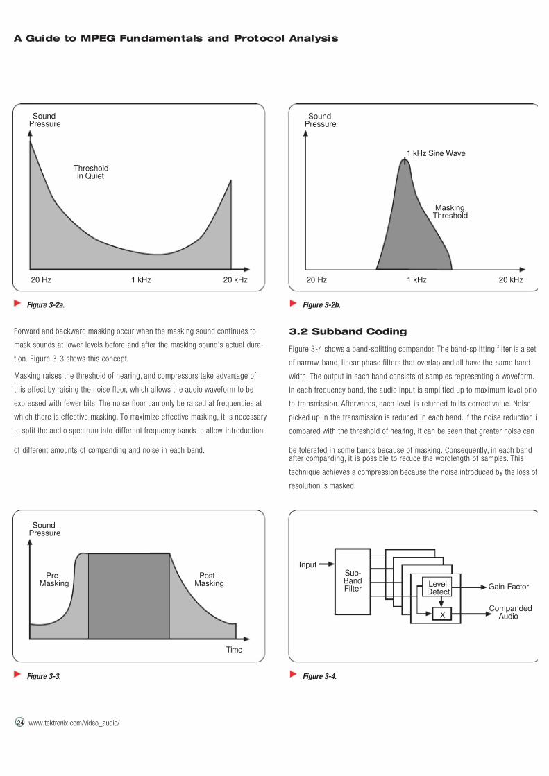
7/16/2019 MPEG Tektronix
http://slidepdf.com/reader/full/mpeg-tektronix 30/64
24
A Guide to MPEG Fundamentals and Protocol Analysis
www.tektronix.com/video_audio/ 24
Forward and backward masking occur when the masking sound continues to
mask sounds at lower levels before and after the masking sound’s actual dura-
tion. Figure 3-3 shows this concept.
Masking raises the threshold of hearing, and compressors take advantage of
this effect by raising the noise floor, which allows the audio waveform to be
expressed with fewer bits. The noise floor can only be raised at frequencies at
which there is effective masking. To maximize effective masking, it is necessary
to split the audio spectrum into different frequency bands to allow introduction
of different amounts of companding and noise in each band.
3.2 Subband Coding
Figure 3-4 shows a band-splitting compandor. The band-splitting filter is a set
of narrow-band, linear-phase filters that overlap and all have the same band-
width. The output in each band consists of samples representing a waveform.
In each frequency band, the audio input is amplified up to maximum level prior
to transmission. Afterwards, each level is returned to its correct value. Noise
picked up in the transmission is reduced in each band. If the noise reduction is
compared with the threshold of hearing, it can be seen that greater noise can
be tolerated in some bands because of masking. Consequently, in each bandafter companding, it is possible to reduce the wordlength of samples. This
technique achieves a compression because the noise introduced by the loss of
resolution is masked.
Figure 3-2a.
SoundPressure
20 Hz
Thresholdin Quiet
1 kHz 20 kHz
Figure 3-2b.
SoundPressure
20 Hz
MaskingThreshold
1 kHz 20 kHz
1 kHz Sine Wave
Figure 3-3.
SoundPressure
Post-Masking
Time
Pre-Masking
Figure 3-4.
Gain Factor
CompandedAudio
InputSub-BandFilter
LevelDetect
X
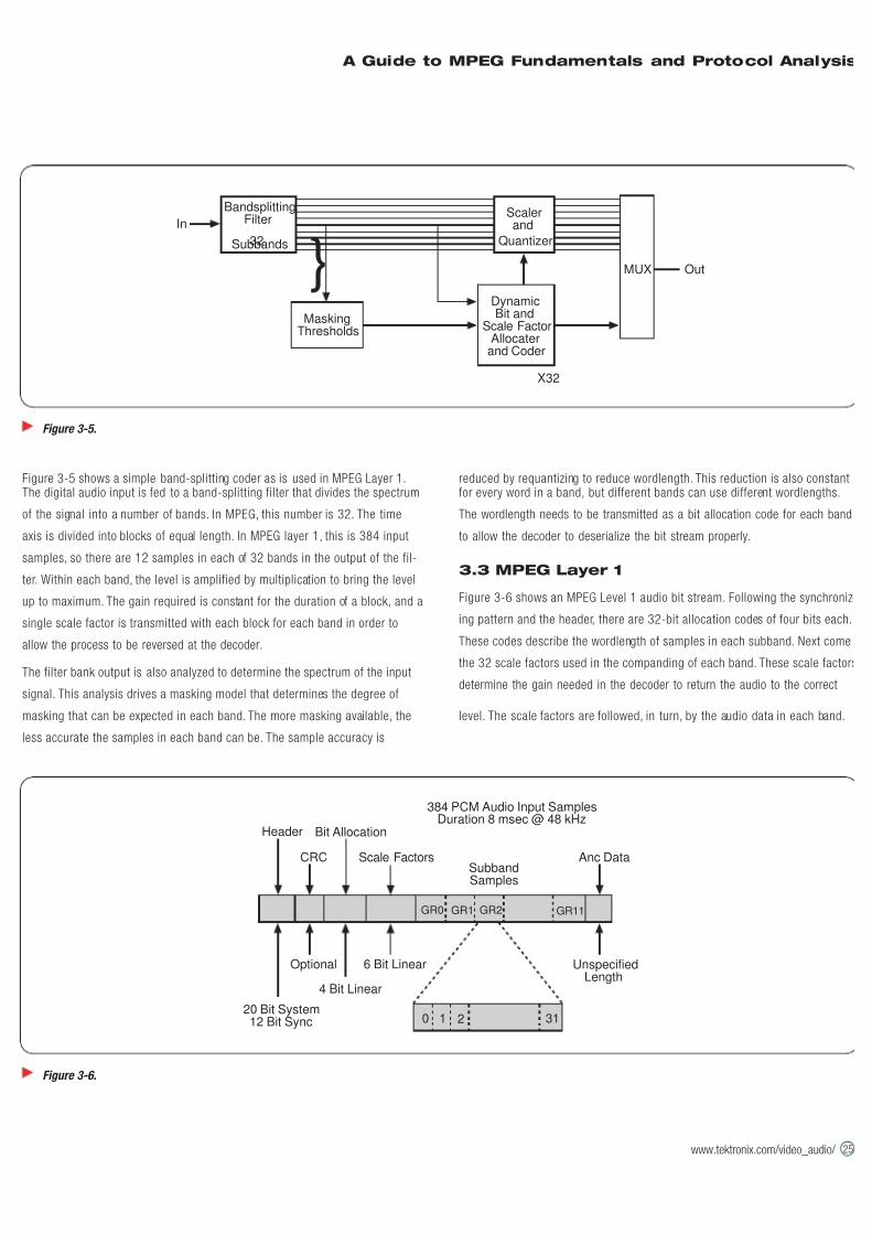
7/16/2019 MPEG Tektronix
http://slidepdf.com/reader/full/mpeg-tektronix 31/64
A Guide to MPEG Fundamentals and Protocol Analysis
www.tektronix.com/video_audio/ 25
Figure 3-5 shows a simple band-splitting coder as is used in MPEG Layer 1.The digital audio input is fed to a band-splitting filter that divides the spectrum
of the signal into a number of bands. In MPEG, this number is 32. The time
axis is divided into blocks of equal length. In MPEG layer 1, this is 384 input
samples, so there are 12 samples in each of 32 bands in the output of the fil-
ter. Within each band, the level is amplified by multiplication to bring the level
up to maximum. The gain required is constant for the duration of a block, and a
single scale factor is transmitted with each block for each band in order to
allow the process to be reversed at the decoder.
The filter bank output is also analyzed to determine the spectrum of the input
signal. This analysis drives a masking model that determines the degree of
masking that can be expected in each band. The more masking available, the
less accurate the samples in each band can be. The sample accuracy is
reduced by requantizing to reduce wordlength. This reduction is also constantfor every word in a band, but different bands can use different wordlengths.
The wordlength needs to be transmitted as a bit allocation code for each band
to allow the decoder to deserialize the bit stream properly.
3.3 MPEG Layer 1
Figure 3-6 shows an MPEG Level 1 audio bit stream. Following the synchroniz-
ing pattern and the header, there are 32-bit allocation codes of four bits each.
These codes describe the wordlength of samples in each subband. Next come
the 32 scale factors used in the companding of each band. These scale factors
determine the gain needed in the decoder to return the audio to the correct
level. The scale factors are followed, in turn, by the audio data in each band.
Figure 3-5.
In
OutMUX
X32
MaskingThresholds
BandsplittingFilter
32Subbands
Scalerand
Quantizer
DynamicBit and
Scale FactorAllocater
and Coder
}
Figure 3-6.
SubbandSamples
384 PCM Audio Input SamplesDuration 8 msec @ 48 kHz
Header
20 Bit System12 Bit Sync
CRC
Optional
Bit Allocation
4 Bit Linear
Scale Factors
6 Bit Linear
Anc Data
UnspecifiedLength
GR0 GR1 GR2 GR11
0 1 2 31
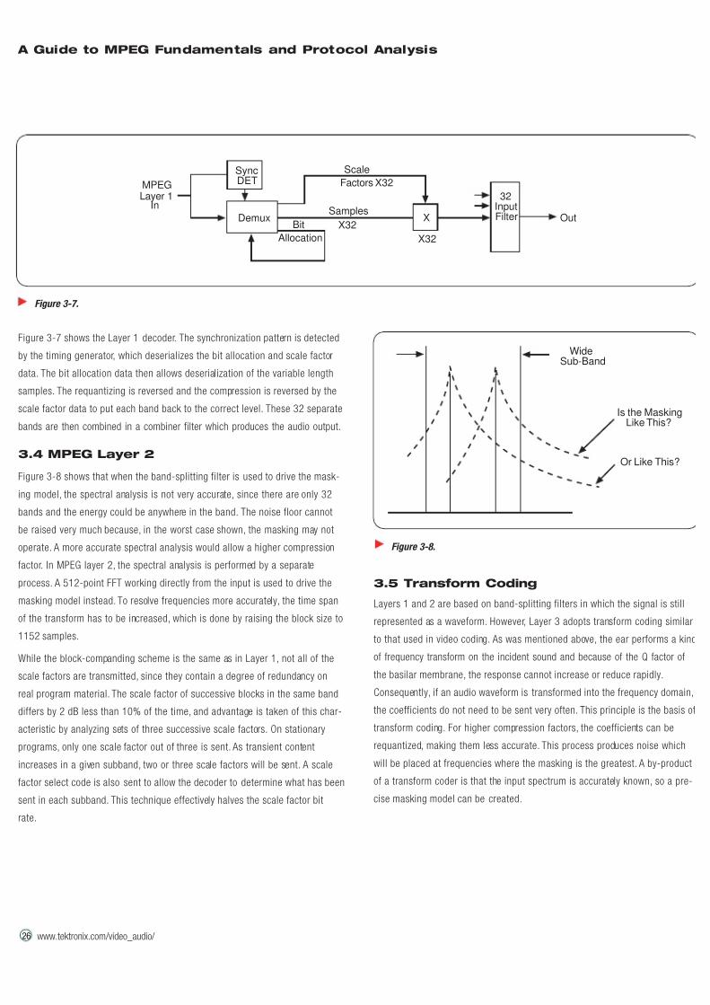
7/16/2019 MPEG Tektronix
http://slidepdf.com/reader/full/mpeg-tektronix 32/64
26
A Guide to MPEG Fundamentals and Protocol Analysis
www.tektronix.com/video_audio/ 26
Figure 3-7 shows the Layer 1 decoder. The synchronization pattern is detected
by the timing generator, which deserializes the bit allocation and scale factor
data. The bit allocation data then allows deserialization of the variable length
samples. The requantizing is reversed and the compression is reversed by the
scale factor data to put each band back to the correct level. These 32 separate
bands are then combined in a combiner filter which produces the audio output.
3.4 MPEG Layer 2
Figure 3-8 shows that when the band-splitting filter is used to drive the mask-
ing model, the spectral analysis is not very accurate, since there are only 32
bands and the energy could be anywhere in the band. The noise floor cannot
be raised very much because, in the worst case shown, the masking may not
operate. A more accurate spectral analysis would allow a higher compression
factor. In MPEG layer 2, the spectral analysis is performed by a separate
process. A 512-point FFT working directly from the input is used to drive the
masking model instead. To resolve frequencies more accurately, the time span
of the transform has to be increased, which is done by raising the block size to
1152 samples.
While the block-companding scheme is the same as in Layer 1, not all of the
scale factors are transmitted, since they contain a degree of redundancy on
real program material. The scale factor of successive blocks in the same band
differs by 2 dB less than 10% of the time, and advantage is taken of this char-
acteristic by analyzing sets of three successive scale factors. On stationary
programs, only one scale factor out of three is sent. As transient content
increases in a given subband, two or three scale factors will be sent. A scale
factor select code is also sent to allow the decoder to determine what has been
sent in each subband. This technique effectively halves the scale factor bit
rate.
3.5 Transform Coding
Layers 1 and 2 are based on band-splitting filters in which the signal is still
represented as a waveform. However, Layer 3 adopts transform coding similar
to that used in video coding. As was mentioned above, the ear performs a kind
of frequency transform on the incident sound and because of the Q factor of
the basilar membrane, the response cannot increase or reduce rapidly.
Consequently, if an audio waveform is transformed into the frequency domain,
the coefficients do not need to be sent very often. This principle is the basis of
transform coding. For higher compression factors, the coefficients can be
requantized, making them less accurate. This process produces noise which
will be placed at frequencies where the masking is the greatest. A by-product
of a transform coder is that the input spectrum is accurately known, so a pre-
cise masking model can be created.
Figure 3-7.
MPEGLayer 1
In
Out
SyncDET
32InputFilterX
Scale
Factors
X32
X32
Samples
X32Bit
Allocation
Demux
Figure 3-8.
WideSub-Band
Is the MaskingLike This?
Or Like This?
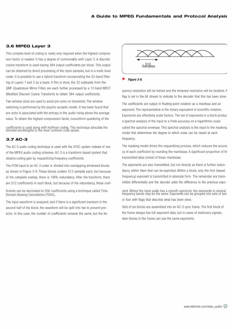
7/16/2019 MPEG Tektronix
http://slidepdf.com/reader/full/mpeg-tektronix 33/64
A Guide to MPEG Fundamentals and Protocol Analysis
www.tektronix.com/video_audio/ 27
3.6 MPEG Layer 3
This complex level of coding is really only required when the highest compres-
sion factor is needed. It has a degree of commonality with Layer 2. A discrete
cosine transform is used having 384 output coefficients per block. This output
can be obtained by direct processing of the input samples, but in a multi-level
coder, it is possible to use a hybrid transform incorporating the 32-band filter-
ing of Layers 1 and 2 as a basis. If this is done, the 32 subbands from the
QMF (Quadrature Mirror Filter) are each further processed by a 12-band MDCT
(Modified Discreet Cosine Transform) to obtain 384 output coefficients.
Two window sizes are used to avoid pre-echo on transients. The window
switching is performed by the psycho-acoustic model. It has been found that
pre-echo is associated with the entropy in the audio rising above the average
value. To obtain the highest compression factor, nonuniform quantizing of the
coefficients is used along with Huffman coding. This technique allocates theshortest wordlengths to the most common code values.
3.7 AC-3
The AC-3 audio coding technique is used with the ATSC system instead of one
of the MPEG audio coding schemes. AC-3 is a transform-based system that
obtains coding gain by requantizing frequency coefficients.
The PCM input to an AC-3 coder is divided into overlapping windowed blocks
as shown in Figure 3-9. These blocks contain 512 samples each, but because
of the complete overlap, there is 100% redundancy. After the transform, there
are 512 coefficients in each block, but because of the redundancy, these coef-
ficients can be decimated to 256 coefficients using a technique called TimeDomain Aliasing Cancellation (TDAC).
The input waveform is analyzed, and if there is a significant transient in the
second half of the block, the waveform will be split into two to prevent pre-
echo. In this case, the number of coefficients remains the same, but the fre-
quency resolution will be halved and the temporal resolution will be doubled. A
flag is set in the bit stream to indicate to the decoder that this has been done.
The coefficients are output in floating-point notation as a mantissa and an
exponent. The representation is the binary equivalent of scientific notation.
Exponents are effectively scale factors. The set of exponents in a block produc
a spectral analysis of the input to a finite accuracy on a logarithmic scale
called the spectral envelope. This spectral analysis is the input to the masking
model that determines the degree to which noise can be raised at each
frequency.
The masking model drives the requantizing process, which reduces the accura
cy of each coefficient by rounding the mantissae. A significant proportion of th
transmitted data consist of these mantissae.
The exponents are also transmitted, but not directly as there is further redun-
dancy within them that can be exploited. Within a block, only the first (lowest
frequency) exponent is transmitted in absolute form. The remainder are trans-
mitted differentially and the decoder adds the difference to the previous expo-
nent. Where the input audio has a smooth spectrum, the exponents in severalfrequency bands may be the same. Exponents can be grouped into sets of two
or four with flags that describe what has been done.
Sets of six blocks are assembled into an AC-3 sync frame. The first block of
the frame always has full exponent data, but in cases of stationary signals,
later blocks in the frame can use the same exponents.
Figure 3-9.
512Samples

7/16/2019 MPEG Tektronix
http://slidepdf.com/reader/full/mpeg-tektronix 34/64
28
A Guide to MPEG Fundamentals and Protocol Analysis
www.tektronix.com/video_audio/ 28
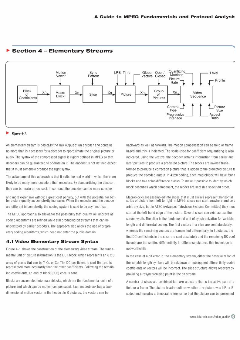
7/16/2019 MPEG Tektronix
http://slidepdf.com/reader/full/mpeg-tektronix 35/64
A Guide to MPEG Fundamentals and Protocol Analysis
www.tektronix.com/video_audio/ 29
An elementa ry stream is basi call y the raw outpu t o f an encode r and conta ins
no more than is necessary for a decoder to approximate the original picture or
audio. The syntax of the compressed signal is rigidly defined in MPEG so that
decoders can be guaranteed to operate on it. The encoder is not defined except
that it must somehow produce the right syntax.
The advantage of this approach is that it suits the real world in which there are
likely to be many more decoders than encoders. By standardizing the decoder,
they can be made at low cost. In contrast, the encoder can be more complex
and more expensive without a great cost penalty, but with the potential for bet-ter picture quality as complexity increases. When the encoder and the decoder
are different in complexity, the coding system is said to be asymmetrical.
The MPEG approach also allows for the possibility that quality will improve as
coding algorithms are refined while still producing bit streams that can be
understood by earlier decoders. The approach also allows the use of propri-
etary coding algorithms, which need not enter the public domain.
4.1 Video Elementary Stream Syntax
Figure 4-1 shows the construction of the elementary video stream. The funda-
mental unit of picture information is the DCT block, which represents an 8 x 8
array of pixels that can be Y, Cr, or Cb. The DC coefficient is sent first and is
represented more accurately than the other coefficients. Following the remain-
ing coefficients, an end of block (EOB) code is sent.
Blocks are assembled into macroblocks, which are the fundamental units of a
picture and which can be motion compensated. Each macroblock has a two-
dimensional motion vector in the header. In B pictures, the vectors can be
backward as well as forward. The motion compensation can be field or frame
based and this is indicated. The scale used for coefficient requantizing is also
indicated. Using the vectors, the decoder obtains information from earlier and
later pictures to produce a predicted picture. The blocks are inverse trans-
formed to produce a correction picture that is added to the predicted picture to
produce the decoded output. In 4:2:0 coding, each macroblock will have four Y
blocks and two color-difference blocks. To make it possible to identify which
block describes which component, the blocks are sent in a specified order.
Macroblocks are assembled into slices that must always represent horizontalstrips of picture from left to right. In MPEG, slices can start anywhere and be o
arbitrary size, but in ATSC (Advanced Television Systems Committee) they must
start at the left-hand edge of the picture. Several slices can exist across the
screen width. The slice is the fundamental unit of synchronization for variable
length and differential coding. The first vectors in a slice are sent absolutely,
whereas the remaining vectors are transmitted differentially. In I pictures, the
first DC coefficients in the slice are sent absolutely and the remaining DC coef
ficients are transmitted differentially. In difference pictures, this technique is
not worthwhile.
In the case of a bit error in the elementary stream, either the deserialization of
the variable length symbols will break down or subsequent differentially-coded
coefficients or vectors will be incorrect. The slice structure allows recovery by
providing a resynchronizing point in the bit stream.
A number of sli ces are combined to make a p ictu re that is the acti ve part of a
field or a frame. The picture header defines whether the picture was I, P, or B
coded and includes a temporal reference so that the picture can be presented
Section 4 – Elementary Streams
Figure 4-1.
MotionVector
SyncPattern
GlobalVectors
PictureSize
AspectRatio
ProgressiveInterlace
ChromaType
QuantizingMatrices
PictureRate
Level
Profile
I.P.B. Time Open/ Closed
XnPictureSlice
MacroBlock
Groupof
Pictures
VideoSequence
Blockof
Coefficients
Xn Xn Xn Xn
7/16/2019 MPEG Tektronix
http://slidepdf.com/reader/full/mpeg-tektronix 36/64
30
A Guide to MPEG Fundamentals and Protocol Analysis
www.tektronix.com/video_audio/ 30
at the correct time. In the case of pans and tilts, the vectors in every macro-
block will be the same. A global vector can be sent for the whole picture, and
the individual vectors then become differences from this global value.
Pictures may be combined to produce a GOP (group of pictures) that must
begin with an I picture. The GOP is the fundamental unit of temporal coding. In
the MPEG standard, the use of a GOP is optional, but it is a practical necessity.
Between I pictures, a variable number of P and/or B pictures may be placed as
was described in Section 2. A GOP may be open or closed. In a closed GOP, the
last B pictures do not require the I picture in the next GOP for decoding and
the bit stream could be cut at the end of the GOP.
If GOPs are used, several GOPs may be combined to produce a video
sequence. The sequence begins with a sequence start code, followed by a
sequence header and ends with a sequence end code. Additional sequence
headers can be placed throughout the sequence. This approach allows decod-ing to begin part way through the sequence, as might happen in playback of
digital video discs and tape cassettes. The sequence header specifies the verti-
cal and horizontal size of the picture, the aspect ratio, the chroma subsampling
format, the picture rate, the use of progressive scan or interlace, the profile,
level, and bit rate, and the quantizing matrices used in intra and inter-coded
pictures.
Without the sequence header data, a decoder cannot understand the bit
stream, and therefore sequence headers become entry points at which
decoders can begin correct operation. The spacing of entry points influences
the delay in correct decoding that occurs when the viewer switches from one
television channel to another.
4.2 Audio Elementary Streams
Various types of audio can be embedded in an MPEG-2 multiplex. These types
include audio coded according to MPEG layers 1, 2, 3, or AC-3. The type of
audio encoding used must be included in a descriptor that a decoder will read
in order to invoke the appropriate type of decoding.
The audio compression process is quite different from the video process. There
is no equivalent to the different I, P, and B frame types, and audio frames
always contain the same amount of audio data. There is no equivalent of bi-
directional coding and audio frames are not transmitted out of sequence.
In MPEG-2 audio, the descriptor in the sequence header contains the layer tha
has been used to compress the audio and the type of compression used (for
example, joint stereo), along with the original sampling rate. The audio
sequence is assembled from a number of access units (AUs) which will be
coded audio frames.
If AC-3 coding is used, as in ATSC, this usage will be reflected in the sequence
header. The audio access unit (AU) is an AC-3 sync frame as described in
Section 3.7. The AC-3 sync frame represents a time span equivalent of 1536
audio samples and will be 32 ms for 48 kHz sampling and 48 ms for 32 kHz.
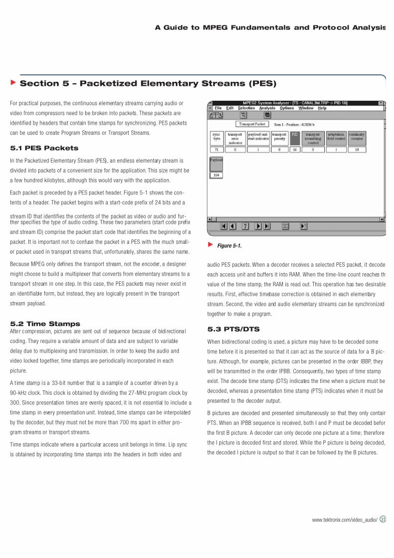
7/16/2019 MPEG Tektronix
http://slidepdf.com/reader/full/mpeg-tektronix 37/64
A Guide to MPEG Fundamentals and Protocol Analysis
www.tektronix.com/video_audio/ 31
For practical purposes, the continuous elementary streams carrying audio or
video from compressors need to be broken into packets. These packets are
identified by headers that contain time stamps for synchronizing. PES packets
can be used to create Program Streams or Transport Streams.
5.1 PES Packets
In the Packetized Elementary Stream (PES), an endless elementary stream is
divided into packets of a convenient size for the application. This size might be
a few hundred kilobytes, although this would vary with the application.
Each packet is preceded by a PES packet header. Figure 5-1 shows the con-
tents of a header. The packet begins with a start-code prefix of 24 bits and a
stream ID that identifies the contents of the packet as video or audio and fur-ther specifies the type of audio coding. These two parameters (start code prefix
and stream ID) comprise the packet start code that identifies the beginning of a
packet. It is important not to confuse the packet in a PES with the much small-
er packet used in transport streams that, unfortunately, shares the same name.
Because MPEG only defines the transport stream, not the encoder, a designer
might choose to build a multiplexer that converts from elementary streams to a
transport stream in one step. In this case, the PES packets may never exist in
an identifiable form, but instead, they are logically present in the transport
stream payload.
5.2 Time Stamps Afte r compressi on, pict ures are sent out of sequence because of bidi rect iona l
coding. They require a variable amount of data and are subject to variable
delay due to multiplexing and transmission. In order to keep the audio and
video locked together, time stamps are periodically incorporated in each
picture.
A t ime stamp i s a 33-b it number that is a sample of a counter driven by a
90-kHz clock. This clock is obtained by dividing the 27-MHz program clock by
300. Since presentation times are evenly spaced, it is not essential to include a
time stamp in every presentation unit. Instead, time stamps can be interpolated
by the decoder, but they must not be more than 700 ms apart in either pro-
gram streams or transport streams.
Time stamps indicate where a particular access unit belongs in time. Lip sync
is obtained by incorporating time stamps into the headers in both video and
audio PES packets. When a decoder receives a selected PES packet, it decodes
each access unit and buffers it into RAM. When the time-line count reaches th
value of the time stamp, the RAM is read out. This operation has two desirable
results. First, effective timebase correction is obtained in each elementary
stream. Second, the video and audio elementary streams can be synchronized
together to make a program.
5.3 PTS/DTS
When bidirectional coding is used, a picture may have to be decoded some
time before it is presented so that it can act as the source of data for a B pic-
ture. Although, for example, pictures can be presented in the order IBBP, they
will be transmitted in the order IPBB. Consequently, two types of time stamp
exist. The decode time stamp (DTS) indicates the time when a picture must be
decoded, whereas a presentation time stamp (PTS) indicates when it must be
presented to the decoder output.
B pictures are decoded and presented simultaneously so that they only contain
PTS. When an IPBB sequence is received, both I and P must be decoded before
the first B picture. A decoder can only decode one picture at a time; therefore
the I picture is decoded first and stored. While the P picture is being decoded,
the decoded I picture is output so that it can be followed by the B pictures.
Section 5 – Packetized Elementary Streams (PES)
Figure 5-1.
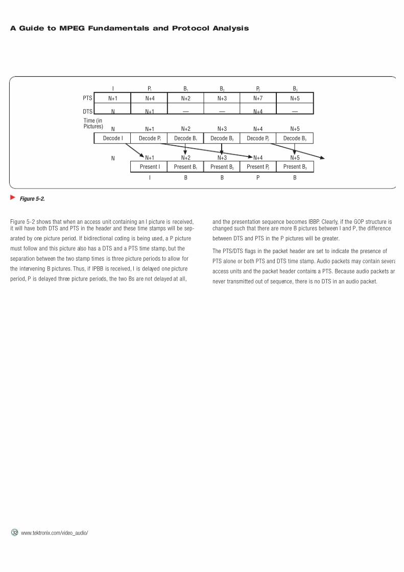
7/16/2019 MPEG Tektronix
http://slidepdf.com/reader/full/mpeg-tektronix 38/64
32
A Guide to MPEG Fundamentals and Protocol Analysis
www.tektronix.com/video_audio/ 32
Figure 5-2 shows that when an access unit containing an I picture is received,it will have both DTS and PTS in the header and these time stamps will be sep-
arated by one picture period. If bidirectional coding is being used, a P picture
must follow and this picture also has a DTS and a PTS time stamp, but the
separation between the two stamp times is three picture periods to allow for
the intervening B pictures. Thus, if IPBB is received, I is delayed one picture
period, P is delayed three picture periods, the two Bs are not delayed at all,
and the presentation sequence becomes IBBP. Clearly, if the GOP structure ischanged such that there are more B pictures between I and P, the difference
between DTS and PTS in the P pictures will be greater.
The PTS/DTS flags in the packet header are set to indicate the presence of
PTS alone or both PTS and DTS time stamp. Audio packets may contain severa
access units and the packet header contains a PTS. Because audio packets are
never transmitted out of sequence, there is no DTS in an audio packet.
Figure 5-2.
PTS
DTS
I P1 P2 B3
N+1 N+4
N+1 N+4
N+2 N+3 N+7 N+5
N — — —
Time (inPictures) N N+1 N+2 N+3 N+4 N+5
Decode I Decode P1 Decode P2 Decode B3Decode B2Decode B1
N N+1 N+2 N+3 N+4 N+5
Present I Present B1 Present B2 Present P2 Present B3
I B B BP
B2B1
7/16/2019 MPEG Tektronix
http://slidepdf.com/reader/full/mpeg-tektronix 39/64
A Guide to MPEG Fundamentals and Protocol Analysis
www.tektronix.com/video_audio/ 33
Program Streams are one way of combining several PES packet streams and
are advantageous for recording applications such as DVD.
6.1 Recording vs. Transmission
For a given picture quality, the data rate of compressed video will vary with pic-
ture content. A variable bit-rate channel will give the best results. In transmis-
sion, most practical channels are fixed and the overall bit-rate is kept constant
by the use of stuffing (meaningless data).
In a DVD, the use of stuffing is a waste of storage capacity. However, a storage
medium can be slowed down or speeded up, either physically or, in the case of
a disk drive, by changing the rate of data transfer requests. This approach
allows a variable-rate channel to be obtained without capacity penalty. When amedium is replayed, the speed can be adjusted to keep a data buffer approxi-
mately half full, irrespective of the actual bit rate which can change dynamical-
ly. If the decoder reads from the buffer at an increased rate, it will tend to
empty the buffer, and the drive system will simply increase the access rate to
restore balance. This technique only works if the audio and video were encoded
from the same clock; otherwise, they will slip over the length of the recording.
To satisfy these conflicting requirements, Program Streams and Transport
Streams have been devised as alternatives. A Program Stream works well on a
single program with variable bit rate in a recording environment; a Transport
Stream works well on multiple programs in a fixed bit-rate transmission
environment.
The problem of genlocking to the source does not occur in a DVD player. The
player determines the time base of the video with a local SPG (internal or
external) and simply obtains data from the disk in order to supply pictures on
that time base. In transmission, the decoder has to recreate the time base at
the encoder or it will suffer overflow or underflow. Thus, a Transport Stream
uses Program Clock Reference (PCR), whereas a Program Stream has no need
for the Program Clock.
6.2 Introduction to Program Streams
A Program S tream i s a PES packet multi plex that carr ies several elementar y
streams that were encoded using the same master clock or system time clock
(STC). This stream might be a video stream and its associated audio streams,
or a multichannel audio-only program. The elementary video stream is divided
into Access Units (AUs), each of which contains compressed data describing
one picture. These pictures are identified as I, P, or B and each carries an
Access Unit number t hat indi cates the correct display sequence. One video
Access Unit becomes one program-stream packe t. In video, these packe ts vary
in size. For example, an I picture packet will be much larger than a B picture
packet. Digital audio Access Units are generally of the same size and several
are assembled into one program-stream packet. These packets should not be
confused with transport-stream packets that are smaller and of fixed size.
Video and audio Access Unit boundaries rarely coincide on the time axis, but
this lack of coincidence is not a problem because each boundary has its own
time-stamp structure.
Section 6 – Program Streams

7/16/2019 MPEG Tektronix
http://slidepdf.com/reader/full/mpeg-tektronix 40/64
34
A Guide to MPEG Fundamentals and Protocol Analysis
www.tektronix.com/video_audio/ 34
7/16/2019 MPEG Tektronix
http://slidepdf.com/reader/full/mpeg-tektronix 41/64
A Guide to MPEG Fundamentals and Protocol Analysis
www.tektronix.com/video_audio/ 35
A t ransport stream i s more than a multi plex of many PES packets. In Program
Streams, time stamps are sufficient to recreate the time axis because the audio
and video are locked to a common clock. For transmission down a data net-
work over distance, there is an additional requirement to recreate the clock for
each program at the decoder. This requires an additional layer of syntax to pro-
vide program clock reference (PCR) signals.
7.1 The Job of a Transport Stream
The transport stream carries many different programs and each may use a dif-
ferent compression factor and a bit rate that can change dynamically even
though the overall bit rate stays constant. This behavior is called statistical
multiplexing and it allows a program that is handling difficult material to borrow
bandwidth from a program handling easy material. Each video PES can have a
different number of audio and data PESs associated with it. Despite this flexi-
bility, a decoder must be able to change from one program to the next and cor-
rectly select the appropriate audio and data channels. Some of the programs
can be protected so that they can only be viewed by those who have paid a
subscription or fee. The transport stream must contain conditional access (CA)
information to administer this protection. The transport stream contains pro-
gram specific information (PSI) to handle these tasks.
The transport layer converts the PES data into small packets of constant size
that are self contained. When these packets arrive at the decoder, there may be
jit ter in the timi ng. The use of time divi sion mult iplexing also causes delay, but
this factor is not fixed because the proportion of the bit stream allocated to
each program is not fixed. Time stamps are part of the solution, but they only
work if a stable clock is available. The transport stream must contain further
data allowing the recreation of a stable clock.
The operation of digital video production equipment is heavily dependent on the
distribution of a stable system clock for synchronization. In video production,
genlocking is used, but over long distances, the distribution of a separate clock
is not practical. In a transport stream, the different programs may have origi-
nated in different places that are not necessarily synchronized. As a result, the
transport stream has to provide a separate means of synchronizing for each
program.
This additional synchronization method is called a Program Clock Reference
(PCR) and it recreates a stable reference clock that can be divided down to
create a time line at the decoder, so that the time stamps for the elementary
streams in each program stream become useful. Consequently, one definition
of a program is a set of elementary streams sharing the same timing
reference.
In a Single Program Transport Stream (SPTS), there will be one PCR channel
that recreates one program clock for both audio and video. The SPTS is often
used as the communication between an audio/video coder and a multiplexer.
Section 7 – Transport Streams
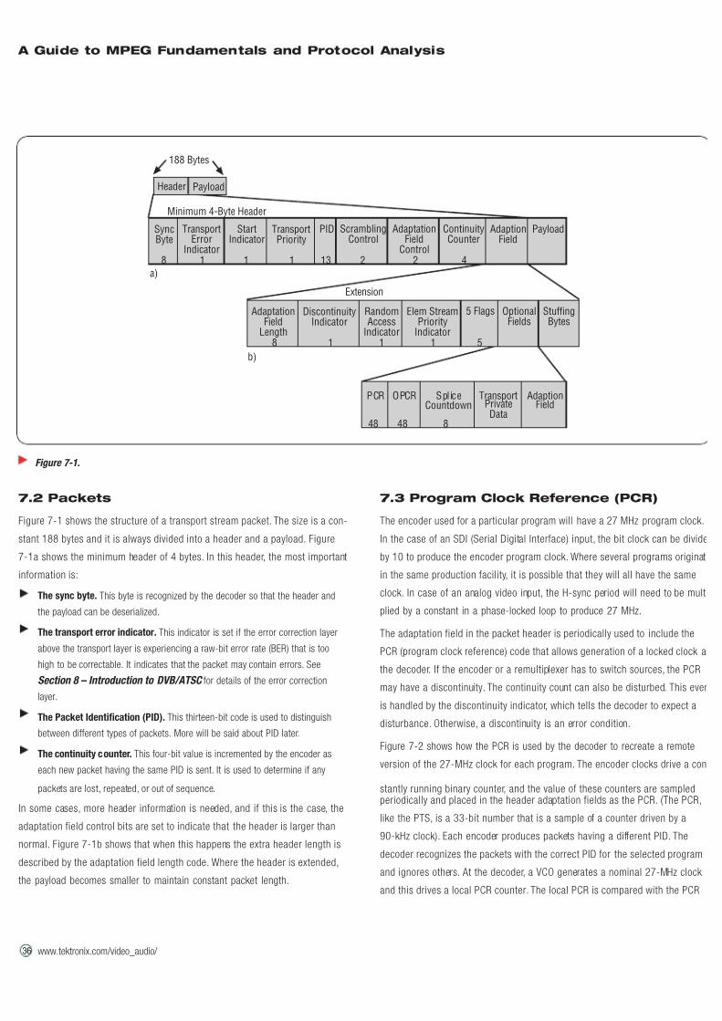
7/16/2019 MPEG Tektronix
http://slidepdf.com/reader/full/mpeg-tektronix 42/64
36
A Guide to MPEG Fundamentals and Protocol Analysis
www.tektronix.com/video_audio/ 36
7.2 Packets
Figure 7-1 shows the structure of a transport stream packet. The size is a con-
stant 188 bytes and it is always divided into a header and a payload. Figure
7-1a shows the minimum header of 4 bytes. In this header, the most important
information is:
The sync byte. This byte is recognized by the decoder so that the header and
the payload can be deserialized.
The transport error indicator. This indicator is set if the error correction layer
above the transport layer is experiencing a raw-bit error rate (BER) that is too
high to be correctable. It indicates that the packet may contain errors. See
Section 8 – Introduction to DVB/ATSC for details of the error correction
layer.
The Packet Identification (PID). This thirteen-bit code is used to distinguish
between different types of packets. More will be said about PID later.
The continuity counter. This four-bit value is incremented by the encoder as
each new packet having the same PID is sent. It is used to determine if any
packets are lost, repeated, or out of sequence.
In some cases, more header information is needed, and if this is the case, the
adaptation field control bits are set to indicate that the header is larger than
normal. Figure 7-1b shows that when this happens the extra header length is
described by the adaptation field length code. Where the header is extended,
the payload becomes smaller to maintain constant packet length.
7.3 Program Clock Reference (PCR)
The encoder used for a particular program will have a 27 MHz program clock.
In the case of an SDI (Serial Digital Interface) input, the bit clock can be divide
by 10 to produce the encoder program clock. Where several programs originate
in the same production facility, it is possible that they will all have the same
clock. In case of an analog video input, the H-sync period will need to be multi
plied by a constant in a phase-locked loop to produce 27 MHz.
The adaptation field in the packet header is periodically used to include the
PCR (program clock reference) code that allows generation of a locked clock at
the decoder. If the encoder or a remultiplexer has to switch sources, the PCR
may have a discontinuity. The continuity count can also be disturbed. This even
is handled by the discontinuity indicator, which tells the decoder to expect a
disturbance. Otherwise, a discontinuity is an error condition.
Figure 7-2 shows how the PCR is used by the decoder to recreate a remote
version of the 27-MHz clock for each program. The encoder clocks drive a con
stantly running binary counter, and the value of these counters are sampledperiodically and placed in the header adaptation fields as the PCR. (The PCR,
like the PTS, is a 33-bit number that is a sample of a counter driven by a
90-kHz clock). Each encoder produces packets having a different PID. The
decoder recognizes the packets with the correct PID for the selected program
and ignores others. At the decoder, a VCO generates a nominal 27-MHz clock
and this drives a local PCR counter. The local PCR is compared with the PCR
Figure 7-1.
a)
b)
188 Bytes
Minimum 4-Byte Header
Header Payload
PCR OPCR SpliceCountdown
TransportPrivateData
AdaptionField
Extension
48 48 8
AdaptationField
Length
DiscontinuityIndicator
RandomAccess
Indicator
Elem StreamPriority
Indicator
5 Flags OptionalFields
StuffingBytes
8 1 1 1 5
SyncByte
TransportError
Indicator
StartIndicator
TransportPriority
PID ScramblingControl
AdaptationField
Control
ContinuityCounter
AdaptionField
Payload
8 1 11 13 2 2 4
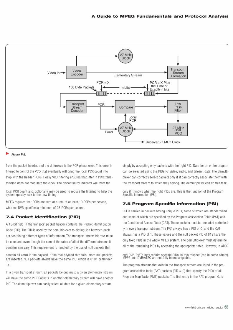
7/16/2019 MPEG Tektronix
http://slidepdf.com/reader/full/mpeg-tektronix 43/64
A Guide to MPEG Fundamentals and Protocol Analysis
www.tektronix.com/video_audio/ 37
from the packet header, and the difference is the PCR phase error. This error is
filtered to control the VCO that eventually will bring the local PCR count into
step with the header PCRs. Heavy VCO filtering ensures that jitter in PCR trans-
mission does not modulate the clock. The discontinuity indicator will reset the
local PCR count and, optionally, may be used to reduce the filtering to help thesystem quickly lock to the new timing.
MPEG requires that PCRs are sent at a rate of at least 10 PCRs per second,
whereas DVB specifies a minimum of 25 PCRs per second.
7.4 Packet Identification (PID)
A 13-bi t f ield in the transpor t packet header contai ns the Packet Iden tifi cati on
Code (PID). The PID is used by the demultiplexer to distinguish between pack-
ets containing different types of information. The transport-stream bit rate must
be constant, even though the sum of the rates of all of the different streams it
contains can vary. This requirement is handled by the use of null packets that
contain all zeros in the payload. If the real payload rate falls, more null packets
are inserted. Null packets always have the same PID, which is 8191 or thirteen
1s.
In a given transport stream, all packets belonging to a given elementary stream
will have the same PID. Packets in another elementary stream will have another
PID. The demultiplexer can easily select all data for a given elementary stream
simply by accepting only packets with the right PID. Data for an entire program
can be selected using the PIDs for video, audio, and teletext data. The demulti-
plexer can correctly select packets only if it can correctly associate them with
the transport stream to which they belong. The demultiplexer can do this task
only if it knows what the right PIDs are. This is the function of the ProgramSpecific Information (PSI).
7.5 Program Specific Information (PSI)
PSI is carried in packets having unique PIDs, some of which are standardized
and some of which are specified by the Program Association Table (PAT) and
the Conditional Access Table (CAT). These packets must be included periodical
ly in every transport stream. The PAT always has a PID of 0, and the CAT
always has a PID of 1. These values and the null packet PID of 8191 are the
only fixed PIDs in the whole MPEG system. The demultiplexer must determine
all of the remaining PIDs by accessing the appropriate table. However, in ATSC
and DVB, PMTs may require specific PIDs. In this respect (and in some others)MPEG and DVB/ATSC are not fully interchangeable.
The program streams that exist in the transport stream are listed in the pro-
gram association table (PAT) packets (PID = 0) that specify the PIDs of all
Program Map Table (PMT) packets. The first entry in the PAT, program 0, is
Figure 7-2.
Video InElementary Stream
188 Byte Packets
PCR = X PCR = X Plusthe Time of
Exactly n bitsn bits
PCR
LocalPCR
Load
Receiver 27 MHz Clock
VideoEncoder
TransportStreamDecoder
27 MHzClock
Compare
TransportStream
Formation
LowPassFilter
27 MHzClock
27 MHzXtalVCO
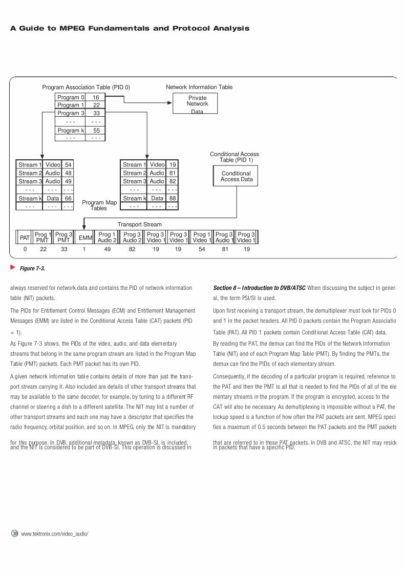
7/16/2019 MPEG Tektronix
http://slidepdf.com/reader/full/mpeg-tektronix 44/64
38
A Guide to MPEG Fundamentals and Protocol Analysis
www.tektronix.com/video_audio/ 38
always reserved for network data and contains the PID of network information
table (NIT) packets.
The PIDs for Entitlement Control Messages (ECM) and Entitlement Management
Messages (EMM) are listed in the Conditional Access Table (CAT) packets (PID
= 1).
As Figure 7-3 shows, the PIDs of the video, audio, and data elementa ry
streams that belong in the same program stream are listed in the Program Map
Table (PMT) packets. Each PMT packet has its own PID.
A g iven network info rmat ion table contai ns detai ls of more than just the trans-
port stream carrying it. Also included are details of other transport streams that
may be available to the same decoder, for example, by tuning to a different RF
channel or steering a dish to a different satellite. The NIT may list a number of
other transport streams and each one may have a descriptor that specifies the
radio frequency, orbital position, and so on. In MPEG, only the NIT is mandatory
for this purpose. In DVB, additional metadata, known as DVB-SI, is included,and the NIT is considered to be part of DVB-SI. This operation is discussed in
Section 8 – Introduction to DVB/ATSC . When discussing the subject in gener-
al, the term PSI/SI is used.
Upon first receiving a transport stream, the demultiplexer must look for PIDs 0
and 1 in the packet headers. All PID 0 packets contain the Program Associatio
Table (PAT). All PID 1 packets contain Condit ional Access Table (CAT) data.
By reading the PAT, the demux can find the PIDs of the Network Information
Table (NIT) and of each Program Map Table (PMT). By finding the PMTs, the
demux can find the PIDs of each elementary stream.
Consequently, if the decoding of a particular program is required, reference to
the PAT and then the PMT is all that is needed to find the PIDs of all of the ele
mentary streams in the program. If the program is encrypted, access to the
CAT will also be necessary. As demultiplexing is impossible without a PAT, the
lockup speed is a function of how often the PAT packets are sent. MPEG speci-
fies a maximum of 0.5 seconds between the PAT packets and the PMT packets
that are referred to in those PAT packets. In DVB and ATSC, the NIT may residein packets that have a specific PID.
Figure 7-3.
Program Association Table (PID 0) Network Information Table
Conditional AccessTable (PID 1)
Program MapTables
Transport Stream
Stream 1 Video 54
Stream 2 Audio 48
Stream 3 Audio 49
Stream k Data 66
- - - - - - - - -
- - - - - - - - -
Stream 1 Video 19
Stream 2 Audio 81
Stream 3 Audio 82
Stream k Data 88
- - - - - - - - -
- - - - - - - - -
PrivateNetwork
Data
ConditionalAccess Data
0
PATProg 1PMT
Prog 3PMT EMM
Prog 1Audio 2
Prog 3Audio 2
Prog 3Video 1
Prog 3Video 1
Prog 1Video 1
Prog 3Audio 1
Prog 3Video 1
22 33 1 49 82 19 19 54 81 19
Program 0 16
Program 1 22
Program 3 33
Program k 55
- - - - - -
- - - - - -
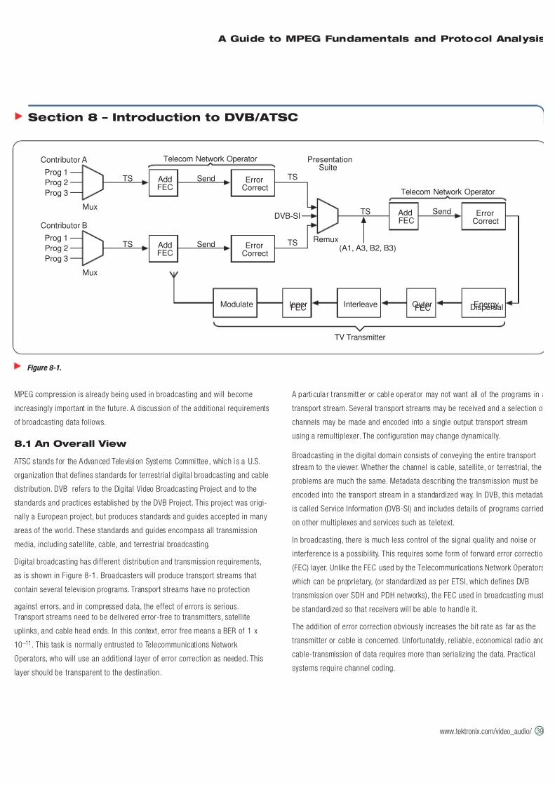
7/16/2019 MPEG Tektronix
http://slidepdf.com/reader/full/mpeg-tektronix 45/64
A Guide to MPEG Fundamentals and Protocol Analysis
www.tektronix.com/video_audio/ 39
MPEG compression is already being used in broadcasting and will become
increasingly important in the future. A discussion of the additional requirements
of broadcasting data follows.
8.1 An Overall View
ATSC s tands for the Advanced Televisi on Systems Commi ttee , which i s a U.S.
organization that defines standards for terrestrial digital broadcasting and cable
distribution. DVB refers to the Digital Video Broadcasting Project and to the
standards and practices established by the DVB Project. This project was origi-
nally a European project, but produces standards and guides accepted in many
areas of the world. These standards and guides encompass all transmission
media, including satellite, cable, and terrestrial broadcasting.
Digital broadcasting has different distribution and transmission requirements,
as is shown in Figure 8-1. Broadcasters will produce transport streams that
contain several television programs. Transport streams have no protection
against errors, and in compressed data, the effect of errors is serious.
Transport streams need to be delivered error-free to transmitters, satellite
uplinks, and cable head ends. In this context, error free means a BER of 1 x
10–11. This task is normally entrusted to Telecommunications Network
Operators, who will use an additional layer of error correction as needed. This
layer should be transparent to the destination.
A parti cula r t ransmitt er or cabl e operator may not want all of the programs in a
transport stream. Several transport streams may be received and a selection of
channels may be made and encoded into a single output transport stream
using a remultiplexer. The configuration may change dynamically.
Broadcasting in the digital domain consists of conveying the entire transport
stream to the viewer. Whether the channel is cable, satellite, or terrestrial, the
problems are much the same. Metadata describing the transmission must be
encoded into the transport stream in a standardized way. In DVB, this metadata
is called Service Information (DVB-SI) and includes details of programs carried
on other multiplexes and services such as teletext.
In broadcasting, there is much less control of the signal quality and noise or
interference is a possibility. This requires some form of forward error correction
(FEC) layer. Unlike the FEC used by the Telecommunications Network Operators
which can be proprietary, (or standardized as per ETSI, which defines DVB
transmission over SDH and PDH networks), the FEC used in broadcasting must
be standardized so that receivers will be able to handle it.
The addition of error correction obviously increases the bit rate as far as the
transmitter or cable is concerned. Unfortunately, reliable, economical radio and
cable-transmission of data requires more than serializing the data. Practical
systems require channel coding.
Section 8 – Introduction to DVB/ATSC
Figure 8-1.
Contributor A
Prog 1
Prog 2
Prog 3
TS TS
TS
Telecom Network Operator
Telecom Network Operator
Send
SendMux
Remux
DVB-SI
(A1, A3, B2, B3)
TV Transmitter
PresentationSuite
AddFEC
ErrorCorrect
ErrorCorrect
Contributor B
Prog 1
Prog 2
Prog 3
TS TSSend
Mux
AddFEC
ErrorCorrect
AddFEC
EnergyDispersalOuterFECInnerFEC InterleaveModulate
7/16/2019 MPEG Tektronix
http://slidepdf.com/reader/full/mpeg-tektronix 46/64
8.2 Remultiplexing
Remultiplexing is a complex task because it has to output a compliant bit
stream that is assembled from parts of others. The required data from a given
input transport stream can be selected with reference to the program associa-
tion table and the program map tables that will disclose the PIDs of the pro-
grams required. It is possible that the same PIDs have been used in two input
transport streams; therefore, the PIDs of one or more elementary streams may
have to be changed. The packet headers must pass on the program clock ref-
erence (PCR) that will allow the final decoder to recreate a 27-MHz clock. As
the position of packets containing PCR may be different in the new multiplex,
the remultiplexer may need to edit the PCR values to reflect their new position
on the time axis.
The program map tables and program association tables will need to be edited
to reflect the new transport stream structure, as will the Conditional AccessTables (CAT).
If the sum of the selected program-stream bit rates is less than the output bit
rate, the remultiplexer will create stuffing packets with suitable PIDs. However,
if the transport streams have come from statistical multiplexers, it is possible
that the instantaneous bit rate of the new transport stream will exceed the
channel capacity. This condition might occur if several selected programs in
different transport streams simultaneously contain high entropy. In this case,
the only solution is to recompress and create new, shorter coefficients in one
or more bit streams to reduce the bit rate.
8.3 Service Information (SI)
In the future, digital delivery will mean that there will be a large number of pro-
grams, teletext, and services available to the viewer and these may be spread
across a number of different transport streams. Both the viewer and the
Integrated Receiver Decoder (IRD) will need help to display what is available
and to output the selected service. This capability requires metadata beyond
the capabilities of MPEG-PSI (Program Specific Information) and is referred to
as DVB-SI (Service Information). DVB-SI is considered to include the NIT, which
must be present in all MPEG transport streams.
DVB-SI is embedded in the transport stream as additional transport packets
with unique PIDs and carries technical information for IRDs. DVB-SI also con-
tains Electronic Program Guide (EPG) information, such as the nature of a pro-
gram, the timing and the channel on which it can be located, and the countries
in which it is available. Programs can also be rated so that parental judgment
can be exercised.
DVB-SI can include the following options over and above MPEG-PSI:
Service Description Table (SDT). Each service in a DVB transport stream can
have a service descriptor and these descriptors are assembled into the Service
Description Table. A service may be television, radio, or teletext. The service
descriptor includes the name of the service provider.
Event Information Table (EIT). EIT is an optional table for DVB which contains
program names, start times, durations, and so on.
Bouquet Association Table (BAT). The BAT is an optional table for DVB that
provides details of bouquets, which are collections of services marketed as a sin-
gle product.
Time and Date Table (TDT). The TDT is an option that embeds a UTC time and
date stamp in the transport stream.
8.4 Error Correction
Error correction is necessary because conditions on long transmission paths
cannot be controlled. In some systems, error detection is sufficient because it
can be used to request a retransmission. Clearly, this approach will not work
with real-time signals such as television. Instead, a system called Forward Erro
Correction (FEC) is used in which sufficient extra bits, known as redundancy,
are added to the data to allow the decoder to perform corrections in real time.
The FEC used in modern systems is usually based on the Reed-Solomon (R-S)
codes. A full discussion of these is outside the scope of this book. Briefly, R-S
codes add redundancy to the data to make a code-word such that when each
symbol is used as a term in a minimum of two simultaneous equations, the
sum (or syndrome) is always zero if there is no error. This zero condition is
obtained irrespective of the data and makes checking easy. In Transport
streams, the packets are always 188 bytes long. The addition of 16 bytes of
R-S redundancy produces a standard FEC code-word of 204 bytes.
40
A Guide to MPEG Fundamentals and Protocol Analysis
www.tektronix.com/video_audio/ 4040
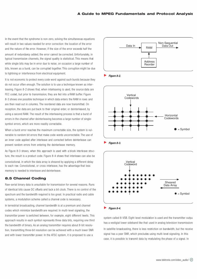
7/16/2019 MPEG Tektronix
http://slidepdf.com/reader/full/mpeg-tektronix 47/64
A Guide to MPEG Fundamentals and Protocol Analysis
www.tektronix.com/video_audio/ 41
In the event that the syndrome is non-zero, solving the simultaneous equations
will result in two values needed for error correction: the location of the error
and the nature of the error. However, if the size of the error exceeds half the
amount of redundancy added, the error cannot be corrected. Unfortunately, in
typical transmission channels, the signal quality is statistical. This means that
while single bits may be in error due to noise, on occasion a large number of
bits, known as a burst, can be corrupted together. This corruption might be due
to lightning or interference from electrical equipment.
It is not economic to protect every code word against such bursts because they
do not occur often enough. The solution is to use a technique known as inter-
leaving. Figure 8-2 shows that, when interleaving is used, the source data are
FEC coded, but prior to transmission, they are fed into a RAM buffer. Figure
8-3 shows one possible technique in which data enters the RAM in rows and
are then read out in columns. The reordered data are now transmitted. On
reception, the data are put back to their original order, or deinterleaved, by
using a second RAM. The result of the interleaving process is that a burst of
errors in the channel after deinterleaving becomes a large number of single-
symbol errors, which are more readily correctable.
When a burst error reaches the maximum correctable size, the system is vul-
nerable to random bit errors that make code-words uncorrectable. The use of
an inner code applied after interleave and corrected before deinterleave can
prevent random errors from entering the deinterleave memory.
As Figure 8-3 shows, when this approach is used with a bl ock inte rleave struc-
ture, the result is a product code. Figure 8-4 shows that interleave can also be
convolutional, in which the data array is sheared by applying a different delay
to each row. Convolutional, or cross interleave, has the advantage that less
memory is needed to interleave and deinterleave.
8.5 Channel Coding
Raw-serial binary data is unsuitable for transmission for several reasons. Runs
of identical bits cause DC offsets and lack a bit clock. There is no control of the
spectrum and the bandwidth required is too great. In practical radio and cable
systems, a modulation scheme called a channel code is necessary.
In terrestrial broadcasting, channel bandwidth is at a premium and channel
codes which minimize bandwidth are required. In multi-level signaling, the
transmitter power is switched between, for example, eight different levels. This
approach results in each symbol represents three data bits, requiring one third
the bandwidth of binary. As an analog transmitter requires about 8-bit resolu-
tion, transmitting three-bit resolution can be achieved with a much lower SNR
and with lower transmitter power. In the ATSC system, it is proposed to use a
system called 8-VSB. Eight-level modulation is used and the transmitter output
has a vestigial lower sideband like that used in analog television transmissions
In satellite broadcasting, there is less restriction on bandwidth, but the receive
signal has a poor SNR, which precludes using multi-level signaling. In this
case, it is possible to transmit data by modulating the phase of a signal. In
Figure 8-2.
Data InNon-Sequential
Data Out
AddressReorder
RAM
Figure 8-3.
VerticalCodewords
HorizontalCodewords
= Symbol
Figure 8-4.
VerticalCodeword
ShearedData Array
= Symbol

7/16/2019 MPEG Tektronix
http://slidepdf.com/reader/full/mpeg-tektronix 48/64
42
A Guide to MPEG Fundamentals and Protocol Analysis
www.tektronix.com/video_audio/ 4242
Phase Shift Keying (PSK), the carrier is transmitted in different phases accord-
ing to the bit pattern. In Quadrature Phase Shift Keying (QPSK), there are four
possible phases. The phases are 90 degrees apart, therefore each symbol car-
ries two bits.
For cable operation, multi-level signaling and phase-shift keying can be com-
bined in Quadrature Amplitude Modulation (QAM), which is a discrete version of
the modulation method used in composite video subcarrier. Figure 8-5 shows
that if two quadrature carriers, known as I and Q, are individually modulated
into eight levels each, the result is a carrier which can have 64 possible combi-
nations of amplitude and phase. Each symbol carries six bits, therefore the
bandwidth required is one third that of QPSK.
In the schemes described above, the transmitted signal spectrum is signal
dependent. Some parts of the spectrum may contain high energy and cause
interference to other services, whereas other parts of the spectrum may con-
tain little energy and be susceptible to interference. In practice, randomizing is
necessary to decorrelate the transmitted spectrum from the data content.
Figure 8-6 shows that when randomizing or energy dispersal is used, a
pseudo-random sequence is added to the serial data before it is input to the
modulator. The result is that the transmitted spectrum is noise-like with rela-
tively stationary statistics. Clearly, an identical and synchronous sequence mus
be subtracted at the receiver as shown. Randomizing cannot be applied to sync
patterns, or they could not be detected.
Figure 8-5.
CarrierIn
4 QuadrantModulator
64 - QuamOut
6 Bits/Symbol
3Bits
DAC
8 Levels
X
90˚Shift
3Bits
DAC
X
8 Levels
+
I
Q
Figure 8-6.
DataIn Data
Out
RandomizedData Transmit
Pseudo-RandomSequenceGenerator
Pseudo-RandomSequenceGenerator
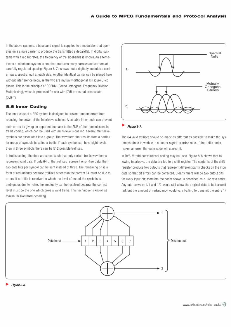
7/16/2019 MPEG Tektronix
http://slidepdf.com/reader/full/mpeg-tektronix 49/64
A Guide to MPEG Fundamentals and Protocol Analysis
www.tektronix.com/video_audio/ 43
In the above systems, a baseband signal is supplied to a modulator that oper-
ates on a single carrier to produce the transmitted sideband(s). In digital sys-
tems with fixed bit rates, the frequency of the sidebands is known. An alterna-
tive to a wideband system is one that produces many narrowband carriers at
carefully regulated spacing. Figure 8-7a shows that a digitally modulated carri-
er has a spectral null at each side. Another identical carrier can be placed here
without interference because the two are mutually orthogonal as Figure 8-7b
shows. This is the principle of COFDM (Coded Orthogonal Frequency Division
Multiplexing), which is proposed for use with DVB terrestrial broadcasts
(DVB-T).
8.6 Inner Coding
The inner code of a FEC system is designed to prevent random errors from
reducing the power of the interleave scheme. A suitable inner code can prevent
such errors by giving an apparent increase to the SNR of the transmission. In
trellis coding, which can be used with multi-level signaling, several multi-level
symbols are associated into a group. The waveform that results from a particu-
lar group of symbols is called a trellis. If each symbol can have eight levels,
then in three symbols there can be 512 possible trellises.
In trellis coding, the data are coded such that only certain trellis waveforms
represent valid data. If only 64 of the trellises represent error-free data, then
two data bits per symbol can be sent instead of three. The remaining bit is a
form of redundancy because trellises other than the correct 64 must be due to
errors. If a trellis is received in which the level of one of the symbols is
ambiguous due to noise, the ambiguity can be resolved because the correct
level must be the one which gives a valid trellis. This technique is known as
maximum-likelihood decoding.
The 64 valid trellises should be made as different as possible to make the sys-
tem continue to work with a poorer signal-to-noise ratio. If the trellis coder
makes an error, the outer code will correct it.
In DVB, Viterbi convolutional coding may be used. Figure 8-8 shows that fol-
lowing interleave, the data are fed to a shift register. The contents of the shift
register produce two outputs that represent different parity checks on the input
data so that bit errors can be corrected. Clearly, there will be two output bits
for every input bit; therefore the coder shown is described as a 1/2 rate coder.
Any rate between 1 /1 and 1/2 would s till all ow the o rigi nal data to be t ransmit
ted, but the amount of redundancy would vary. Failing to transmit the entire 1/
Figure 8-7.
SpectralNulls
MutuallyOrthogonal
Carriers
a)
b)
Figure 8-8.
Data input Data output1 2 3 4 5 6 7
1
2
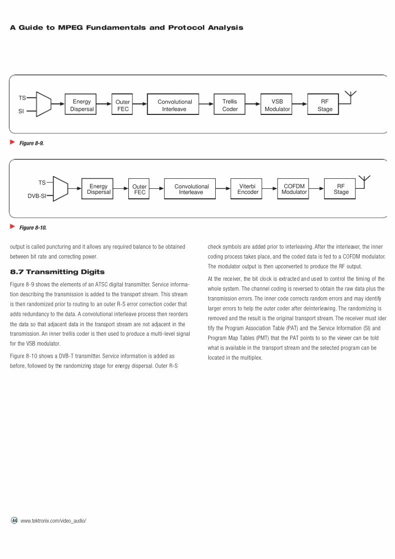
7/16/2019 MPEG Tektronix
http://slidepdf.com/reader/full/mpeg-tektronix 50/64
44
A Guide to MPEG Fundamentals and Protocol Analysis
www.tektronix.com/video_audio/ 4444
output is called puncturing and it allows any required balance to be obtained
between bit rate and correcting power.
8.7 Transmitting Digits
Figure 8-9 shows the elements of an ATSC digital transmitter. Service informa-
tion describing the transmission is added to the transport stream. This stream
is then randomized prior to routing to an outer R-S error correction coder that
adds redundancy to the data. A convolutional interleave process then reorders
the data so that adjacent data in the transport stream are not adjacent in the
transmission. An inner trellis coder is then used to produce a multi-level signal
for the VSB modulator.
Figure 8-10 shows a DVB-T transmitter. Service information is added as
before, followed by the randomizing stage for energy dispersal. Outer R-S
check symbols are added prior to interleaving. After the interleaver, the inner
coding process takes place, and the coded data is fed to a COFDM modulator.
The modulator output is then upconverted to produce the RF output.
At the rece iver, the bit clock is extracted and used to cont rol the timi ng of the
whole system. The channel coding is reversed to obtain the raw data plus the
transmission errors. The inner code corrects random errors and may identify
larger errors to help the outer coder after deinterleaving. The randomizing is
removed and the result is the original transport stream. The receiver must iden
tify the Program Association Table (PAT) and the Service Information (SI) and
Program Map Tables (PMT) that the PAT points to so the viewer can be told
what is available in the transport stream and the selected program can be
located in the multiplex.
Figure 8-9.
Energy
Dispersal
RF
Stage
TS
SI
Outer
FEC
VSB
Modulator
Convolutional
Interleave
Trellis
Coder
Figure 8-10.
EnergyDispersal
RFStage
TS
DVB-SI
OuterFEC
ConvolutionalInterleave
ViterbiEncoder
COFDMModulator
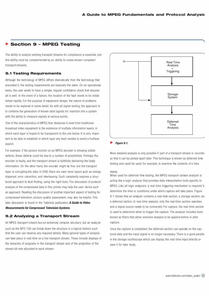
7/16/2019 MPEG Tektronix
http://slidepdf.com/reader/full/mpeg-tektronix 51/64
A Guide to MPEG Fundamentals and Protocol Analysis
www.tektronix.com/video_audio/ 45
The ability to analyze existing transport streams for compliance is essential, but
this ability must be complemented by an ability to create known-compliant
transport streams.
9.1 Testing Requirements
Although the technology of MPEG diff ers dramatically from the technology that
preceded it, the testing requirements are basically the same. On an operational
basis, the user wants to have a simple, regular confidence check that ensures
all is well. In the event of a failure, the location of the fault needs to be estab-
lished rapidly. For the purpose of equipment design, the nature of problems
needs to be explored in some detail. As with all signal testing, the approach is
to combine the generation of known valid signals for insertion into a system
with the ability to measure signals at various points.
One of the characteristics of MPEG that distances it most from traditional
broadcast video equipment is the existence of multiple information layers, in
which each layer is hoped to be transparent to the one below. It is very impor-
tant to be able to establish in which layer any fault resides to avoid a fruitless
search.
For example, if the picture monitor on an MPEG decoder is showing visible
defects, these defects could be due to a number of possibilities. Perhaps the
encoder is faulty, and the transport stream is faithfully delivering the faulty
information. On the other hand, the encoder might be fine, but the transport
layer is corrupting the data. In DVB, there are even more layers such as energy
dispersal, error correction, and interleaving. Such complexity requires a struc-
tured approach to fault finding, using the right tools. The discussion of protocol
analysis of the compressed data in this primer may help the user derive such
an approach. Reading the discussion of another important aspect of testing for
compressed television, picture-quality assessment, may also be helpful. This
later discussion is found in the Tektronix publication, A Guide to Video
Measurements for Compressed Television Systems .
9.2 Analyzing a Transport Stream
An MPEG transpor t s tream has an ex tremely complex structure, but an analy zer
such as the MTS 100 can break down the structure in a logical fashion such
that the user can observe any required details. Many general types of analysis
can take place in real time on a live transport stream. These include displays of
the hierarchy of programs in the transport stream and of the proportion of the
stream bit rate allocated to each stream.
More detailed analysis is only possible if part of a transport stream is recorded
so that it can be picked apart later. This technique is known as deferred-time
testing and could be used, for example, to examine the contents of a time
stamp.
When used for deferred-time testing, the MPEG transport-stream analyzer is
acting like a logic analyzer that provides data-interpretation tools specific to
MPEG. Like all logic analyzers, a real-time triggering mechanism is required to
determine the time or conditions under which capture will take place. Figure
9-1 shows that an analyzer contains a real-time section, a storage section, and
a deferred section. In real-time analysis, only the real-time section operates,
and a signal source needs to be connected. For capture, the real-time section
is used to determine when to trigger the capture. The analyzer includes tools
known as filters that allow selective analysis to be applied before or after
capture.
Once the capture is completed, the deferred section can operate on the cap-
tured data and the input signal is no longer necessary. There is a good parallel
in the storage oscilloscope which can display the real-time input directly or
save it for later study.
Section 9 – MPEG Testing
Figure 9-1.
Real TimeAnalysis
+Triggering
DeferredTime
Analysis
StorageSystem
In
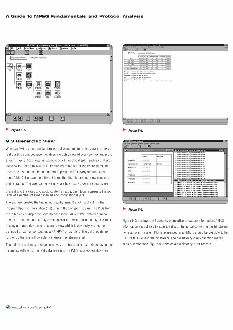
7/16/2019 MPEG Tektronix
http://slidepdf.com/reader/full/mpeg-tektronix 52/64
46
A Guide to MPEG Fundamentals and Protocol Analysis
www.tektronix.com/video_audio/ 464646
9.3 Hierarchic View
When analyzing an unfamiliar transport stream, the hierarchic view is an excel-
lent starting point because it enables a graphic view of every component in the
stream. Figure 9-2 shows an example of a hierarchic display such as that pro-
vided by the Tektronix MTS 200. Beginning at top left of the entire transport
stream, the stream splits and an icon is presented for every stream compo-
nent. Table 9-1 shows the different icons that the hierarchical view uses and
their meaning. The user can very easily see how many program streams are
present and the video and audio content of each. Each icon represents the toplayer of a number of lower analysis and information layers.
The analyzer creates the hierarchic view by using the PAT and PMT in the
Program Specific Information (PSI) data in the transport stream. The PIDs from
these tables are displayed beneath each icon. PAT and PMT data are funda-
mental to the operation of any demultiplexer or decoder; if the analyzer cannot
display a hierarchic view or displays a view which is obviously wrong, the
transport stream under test has a PAT/PMT error. It is unlikely that equipment
further up the line will be able to interpret the stream at all.
The ability of a demux or decoder to lock to a transport stream depends on the
frequency with which the PSI data are sent. The PSI/SI rate option shown in
Figure 9-3 displays the frequency of insertion of system information. PSI/SI
information should also be consistent with the actual content in the bit stream.
For example, if a given PID is referenced in a PMT, it should be possible to find
PIDs of this value in the bit stream. The consistency-check function makes
such a comparison. Figure 9-4 shows a consistency-error readout.
Figure 9-2. Figure 9-3.
Figure 9-4.
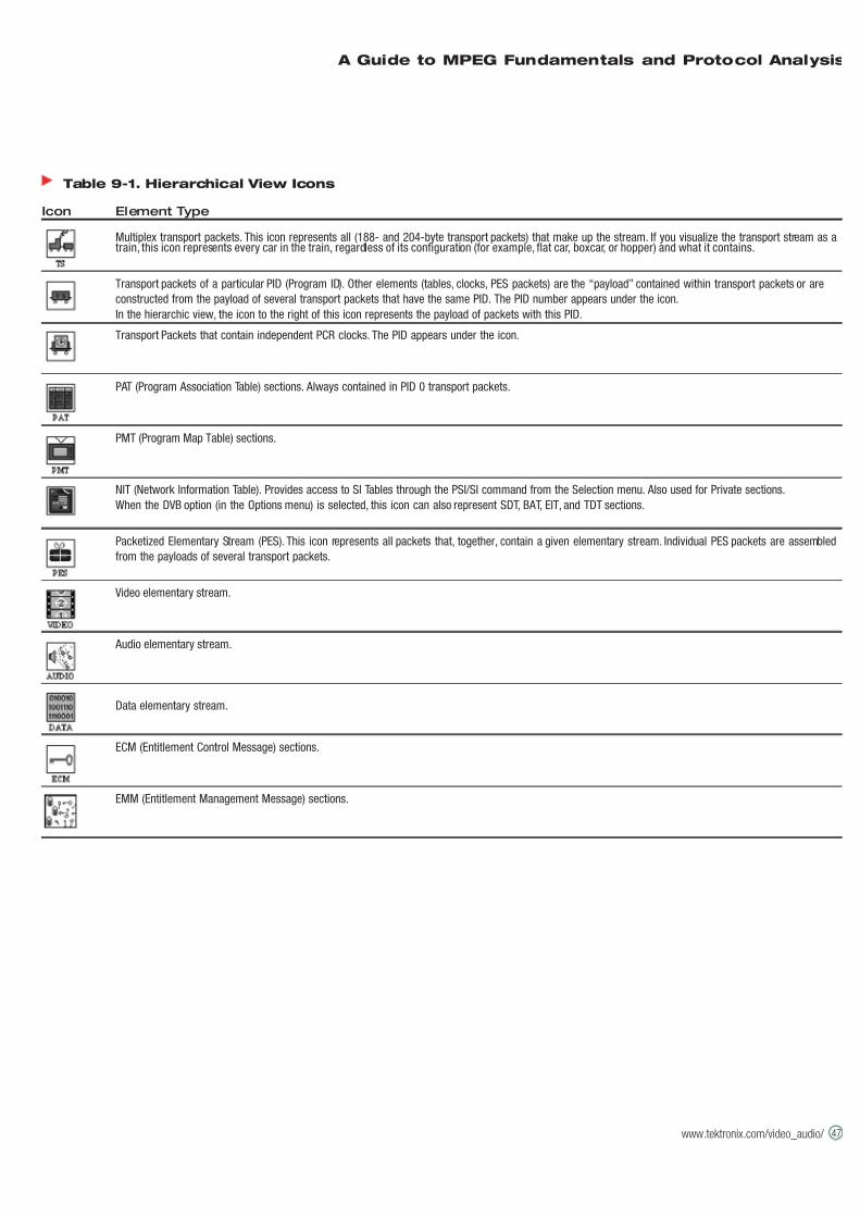
7/16/2019 MPEG Tektronix
http://slidepdf.com/reader/full/mpeg-tektronix 53/64
A Guide to MPEG Fundamentals and Protocol Analysis
www.tektronix.com/video_audio/ 47
Table 9-1. Hierarchical View Icons
Icon Element Type
Multiplex transport packets. This icon represents all (188- and 204-byte transport packets) that make up the stream. If you visualize the transport stream as atrain, this icon represents every car in the train, regardless of its configuration (for example, flat car, boxcar, or hopper) and what it contains.
Transport packets of a particular PID (Program ID). Other elements (tables, clocks, PES packets) are the “payload” contained within transport packets or are
constructed from the payload of several transport packets that have the same PID. The PID number appears under the icon.
In the hierarchic view, the icon to the right of this icon represents the payload of packets with this PID.
Transport Packets that contain independent PCR clocks. The PID appears under the icon.
PAT (Program Association Table) sections. Always contained in PID 0 transport packets.
PMT (Program Map Table) sections.
NIT (Network Information Table). Provides access to SI Tables through the PSI/SI command from the Selection menu. Also used for Private sections.
When the DVB option (in the Options menu) is selected, this icon can also represent SDT, BAT, EIT, and TDT sections.
Packetized Elementary Stream (PES). This icon represents all packets that, together, contain a given elementary stream. Individual PES packets are assembled
from the payloads of several transport packets.
Video elementary stream.
Audio elementary stream.
Data elementary stream.
ECM (Entitlement Control Message) sections.
EMM (Entitlement Management Message) sections.
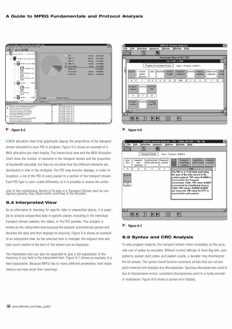
7/16/2019 MPEG Tektronix
http://slidepdf.com/reader/full/mpeg-tektronix 54/64
48
A Guide to MPEG Fundamentals and Protocol Analysis
www.tektronix.com/video_audio/ 484848
A MUX allocati on char t may graphica lly disp lay the propo rtions of t he transpor t
stream allocated to each PID or program. Figure 9-5 shows an example of a
MUX-allocation pie-chart display. The hierarchical view and the MUX Allocation
Chart show the number of elements in the transport stream and the proportion
of bandwidth allocated, but they do not show how the different elements are
distributed in time in the multiplex. The PID map function displays, in order of
reception, a list of the PID of every packet in a section of the transport stream.
Each PID type is color-coded differently, so it is possible to assess the unifor-
mity of the multiplexing. Bursts of SI data in a Transport Stream, sent as con-tiguous packets, may cause buffer overflows in the decoder.
9.4 Interpreted View
As an a lternati ve to checking for spec ific data in unspecif ied places, it is poss i-
ble to analyze unspecified data in specific places, including in the individual
transport stream packets, the tables, or the PES packets. This analysis is
known as the interpreted view because the analyzer automatically parses and
decodes the data and then displays its meaning. Figure 9-6 shows an example
of an interpreted view. As the selected item is changed, the elapsed time and
byte count relative to the start of the stream can be displayed.
The interpreted view can also be expanded to give a full explanation of themeaning of any field in the interpreted item. Figure 9-7 shows an example of a
field explanation. Because MPEG has so many different parameters, field expla-
nations can help recall their meanings.
9.5 Syntax and CRC Analysis
To ship program material, the transport stream relies completely on the accu-
rate use of syntax by encoders. Without correct settings of fixed flag bits, sync
patterns, packet-start codes, and packet counts, a decoder may misinterpret
the bit stream. The syntax check function considers all bits that are not pro-
gram material and displays any discrepancies. Spurious discrepancies could be
due to transmission errors; consistent discrepancies point to a faulty encoder
or multiplexer. Figure 9-8 shows a syntax-error display.
Figure 9-5. Figure 9-6.
Figure 9-7.
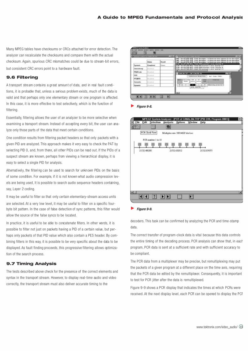
7/16/2019 MPEG Tektronix
http://slidepdf.com/reader/full/mpeg-tektronix 55/64
A Guide to MPEG Fundamentals and Protocol Analysis
www.tektronix.com/video_audio/ 49
Many MPEG tables have checksums or CRCs attached for error detection. The
analyzer can recalculate the checksums and compare them with the actual
checksum. Again, spurious CRC mismatches could be due to stream-bit errors,
but consistent CRC errors point to a hardware fault.
9.6 Filtering
A t ransport stream conta ins a great amoun t o f data, and in real faul t condi -
tions, it is probable that, unless a serious problem exists, much of the data is
valid and that perhaps only one elementary stream or one program is affected.
In this case, it is more effective to test selectively, which is the function of
filtering.
Essentially, filtering allows the user of an analyzer to be more selective when
examining a transport stream. Instead of accepting every bit, the user can ana-
lyze only those parts of the data that meet certain conditions.
One condition results from filtering packet headers so that only packets with a
given PID are analyzed. This approach makes it very easy to check the PAT by
selecting PID 0, and, from there, all other PIDs can be read out. If the PIDs of a
suspect stream are known, perhaps from viewing a hierarchical display, it is
easy to select a single PID for analysis.
Alternat ivel y, the fil teri ng can be used to search for unknown PIDs on the basi s
of some condition. For example, if it is not known what audio compression lev-
els are being used, it is possible to search audio sequence headers containing,
say, Layer 2 coding.
It may be useful to filter so that only certain elementary-stream access units
are selected. At a very low level, it may be useful to filter on a specific four-
byte bit pattern. In the case of false detection of sync patterns, this filter would
allow the source of the false syncs to be located.
In practice, it is useful to be able to concatenate filters. In other words, it is
possible to filter not just on packets having a PID of a certain value, but per-
haps only packets of that PID value which also contain a PES header. By com-
bining filters in this way, it is possible to be very specific about the data to be
displayed. As fault finding proceeds, this progressive filtering allows optimiza-
tion of the search process.
9.7 Timing Analysis
The tests described above check for the presence of the correct elements and
syntax in the transport stream. However, to display real-time audio and video
correctly, the transport stream must also deliver accurate timing to the
decoders. This task can be confirmed by analyzing the PCR and time-stamp
data.
The correct transfer of program-clock data is vital because this data controls
the entire timing of the decoding process. PCR analysis can show that, in each
program, PCR data is sent at a sufficient rate and with sufficient accuracy to
be compliant.
The PCR data from a multiplexer may be precise, but remultiplexing may put
the packets of a given program at a different place on the time axis, requiring
that the PCR data be edited by the remultiplexer. Consequently, it is important
to test for PCR jitter after the data is remultiplexed.
Figure 9-9 shows a PCR display that indicates the times at which PCRs were
received. At the next display level, each PCR can be opened to display the PCR
Figure 9-8.
Figure 9-9.
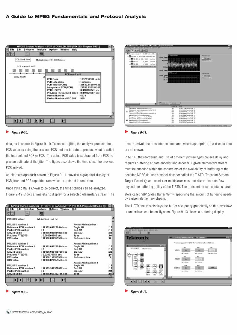
7/16/2019 MPEG Tektronix
http://slidepdf.com/reader/full/mpeg-tektronix 56/64
50
A Guide to MPEG Fundamentals and Protocol Analysis
www.tektronix.com/video_audio/ 505050
data, as is shown in Figure 9-10. To measure jitter, the analyzer predicts the
PCR value by using the previous PCR and the bit rate to produce what is called
the interpolated PCR or PCRI. The actual PCR value is subtracted from PCRI to
give an estimate of the jitter. The figure also shows the time since the previous
PCR arrived.
An alte rnate approach shown in F igure 9-11 prov ides a g raph ical disp lay of
PCR jitter and PCR repetition rate which is updated in real-time.
Once PCR data is known to be correct, the time stamps can be analyzed.
Figure 9-12 shows a time-stamp display for a selected elementary stream. The
time of arrival, the presentation time, and, where appropriate, the decode times
are all shown.
In MPEG, the reordering and use of different picture types causes delay and
requires buffering at both encoder and decoder. A given elementary stream
must be encoded within the constraints of the availability of buffering at the
decoder. MPEG defines a model decoder called the T-STD (Transport Stream
Target Decoder); an encoder or multiplexer must not distort the data flow
beyond the buffering ability of the T-STD. The transport stream contains param
eters called VBV (Video Buffer Verify) specifying the amount of buffering needed
by a given elementary stream.
The T-STD analysis displays the buffer occupancy graphically so that overflows
or underflows can be easily seen. Figure 9-13 shows a buffering display.
Figure 9-10. Figure 9-11.
Figure 9-12. Figure 9-13.
7/16/2019 MPEG Tektronix
http://slidepdf.com/reader/full/mpeg-tektronix 57/64
A Guide to MPEG Fundamentals and Protocol Analysis
www.tektronix.com/video_audio/ 51
The output of a normal compressor/multiplexer is of limited use because it is
not deterministic. If a decoder defect is seen, there is no guarantee that the
same defect will be seen on a repeat of the test because the same video signal
will not result in the same transport stream. In this case, an absolutely repeat-
able transport stream is essential so that the defect can be made to occur at
will for study or rectification.
Transport stream jitter should be within certain limits, but a well-designed
decoder should be able to recover programs beyond this limit in order to guar-
antee reliable operation. There is no way to test for this capability using exist-
ing transport streams because, if they are compliant, the decoder is not being
tested. If there is a failure, it will not be reproducible and it may not be clear
whether the failure was due to jitter or some other noncompliance. The solution
is to generate a transport stream that is compliant in every respect and then
add a controlled amount of jitter to it so that jitter is then known to be the only
source of noncompliance. The multiplexer feature of the MTS 200 is designed
to create such signals.
9.8 Elementary Stream Testing
Because of the flexible nature of the MPEG bit stream, the number of possibili-
ties and combinations it can contain is almost incalculable. As the encoder is
not defined, encoder manufacturers are not compelled to use every possibility;
indeed, for economic reasons, this is unlikely. This fact makes testing quite dif-
ficult because the fact that a decoder works with a particular encoder does not
prove compliance. That decoder may simply not be using the modes that cause
the decoder to fail.
A f urther complication occurs because encoders are not dete rmin ist ic and will
not produce the same bit stream if the video or audio input is repeated. There
is little chance that the same alignment will exist between I, P, and B pictures
and the video frames. If a decoder fails a given test, it may not fail the next
time the test is run, making fault-finding difficult. A failure with a given encoder
does not determine whether the fault lies with the encoder or the decoder. The
coding difficulty depends heavily on the nature of the program material, and
any given program material will not necessarily exercise every parameter over
the whole coding range.
To make tests that have meaningful results, two tools are required:
A known source o f compliant test signals that deliberately explore the whole cod-
ing range. These signals must be deterministic so that a decoder failure will give
repeatable symptoms. The Sarnoff compliant bit streams are designed to perform
this task.
An elementary stream analyzer that allows the entire syntax from an encoder to
be checked for compliance.
9.9 Sarnoff Compliant Bit Streams
These bit streams have been specifically designed by the David Sarnoff
Research Center for decoder compliance testing. They can be multiplexed into
a transport stream feeding a decoder.
No access to the internal working of the decoder is required. To avoid the need
for lengthy analysis of the decoder output, the bit streams have been designed
to create a plain picture when they complete so that it is only necessary to
connect a picture monitor to the decoder output to view them.
There are a number of these simple pictures. Figure 9-14 shows the gray verif
screen. The user should examine the verify screen to look for discrepanciesthat will display well against the gray field. There are also some verify pictures
which are not gray.
Some tests will result in no picture at all if there is a failure. These tests dis-
play the word “VERIFY” on screen when they complete.
Further tests require the viewer to check for smooth motion of a moving ele-
ment across the picture. Timing or ordering problems will cause visible jitter.
The suite of Sarnoff tests may be used to check all of the MPEG syntax ele-
ments in turn. In one test, the bit stream begins with I pictures only, adds P
pictures, and then adds B pictures to test whether all MPEG picture types can
be handled and correctly reordered. Backward compatibility with MPEG-1 canbe proven. Another bit-stream tests using a range of different GOP structures.
There are tests that check the operation of motion vectors over the whole
range of values, and there are tests that vary the size of slices or the amount
of stuffing.
Figure 9-14.
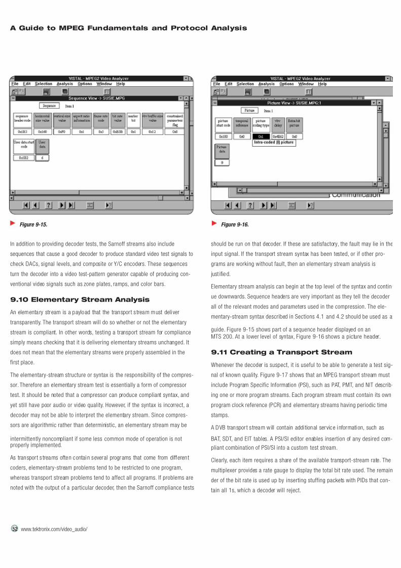
7/16/2019 MPEG Tektronix
http://slidepdf.com/reader/full/mpeg-tektronix 58/64
52
A Guide to MPEG Fundamentals and Protocol Analysis
www.tektronix.com/video_audio/ 525252
In addition to providing decoder tests, the Sarnoff streams also include
sequences that cause a good decoder to produce standard video test signals to
check DACs, signal levels, and composite or Y/C encoders. These sequences
turn the decoder into a video test-pattern generator capable of producing con-
ventional video signals such as zone plates, ramps, and color bars.
9.10 Elementary Stream Analysis
An elementa ry stream is a payload that the transpor t s tream must deli ver
transparently. The transport stream will do so whether or not the elementary
stream is compliant. In other words, testing a transport stream for compliance
simply means checking that it is delivering elementary streams unchanged. It
does not mean that the elementary streams were properly assembled in the
first place.
The elementary-stream structure or syntax is the responsibility of the compres-
sor. Therefore an elementary stream test is essentially a form of compressor
test. It should be noted that a compressor can produce compliant syntax, and
yet still have poor audio or video quality. However, if the syntax is incorrect, a
decoder may not be able to interpret the elementary stream. Since compres-
sors are algorithmic rather than deterministic, an elementary stream may be
intermittently noncompliant if some less common mode of operation is notproperly implemented.
As transpor t s treams often contai n several programs that come from differen t
coders, elementary-stream problems tend to be restricted to one program,
whereas transport stream problems tend to affect all programs. If problems are
noted with the output of a particular decoder, then the Sarnoff compliance tests
should be run on that decoder. If these are satisfactory, the fault may lie in the
input signal. If the transport stream syntax has been tested, or if other pro-
grams are working without fault, then an elementary stream analysis is
just ifie d.
Elementary stream analysis can begin at the top level of the syntax and contin-
ue downwards. Sequence headers are very important as they tell the decoder
all of the relevant modes and parameters used in the compression. The ele-
mentary-stream syntax described in Sections 4.1 and 4.2 should be used as a
guide. Figure 9-15 shows part of a sequence header displayed on an
MTS 200. At a lower level of syntax, Figure 9-16 shows a picture header.
9.11 Creating a Transport Stream
Whenever the decoder is suspect, it is useful to be able to generate a test sig-
nal of known quality. Figure 9-17 shows that an MPEG transport stream must
include Program Specific Information (PSI), such as PAT, PMT, and NIT describ-
ing one or more program streams. Each program stream must contain its own
program clock reference (PCR) and elementary streams having periodic time
stamps.
A DVB transpor t s tream will contain addi tional service i nformation, such as
BAT, SDT, and EIT tables. A PSI/SI editor enables insertion of any desired com-
pliant combination of PSI/SI into a custom test stream.
Clearly, each item requires a share of the available transport-stream rate. The
multiplexer provides a rate gauge to display the total bit rate used. The remain
der of the bit rate is used up by inserting stuffing packets with PIDs that con-
tain all 1s, which a decoder will reject.
Figure 9-15. Figure 9-16.
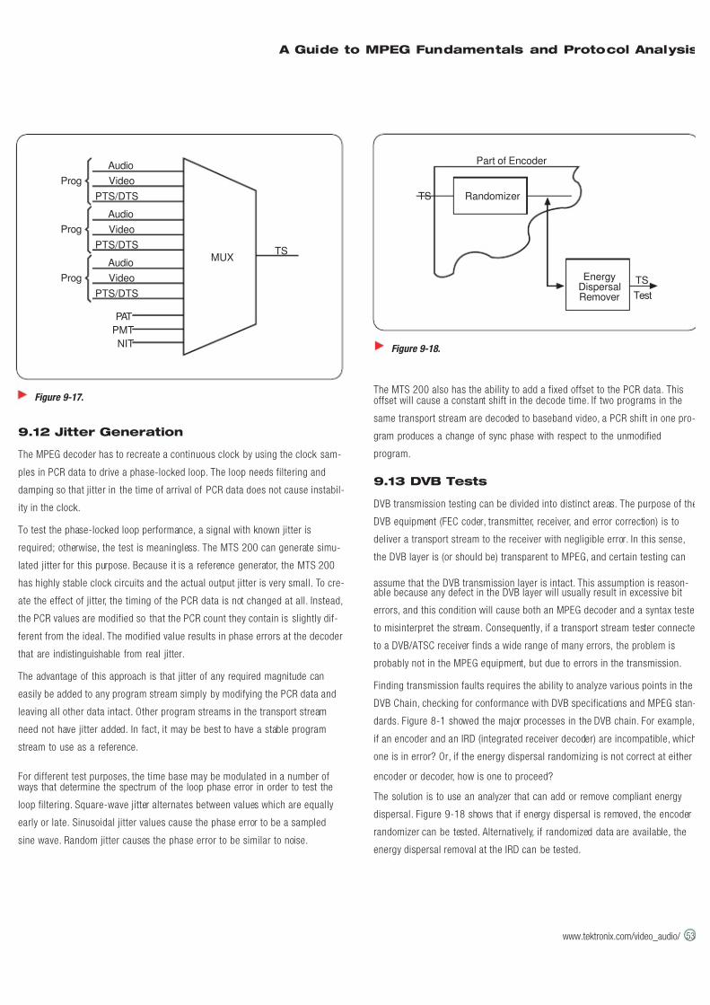
7/16/2019 MPEG Tektronix
http://slidepdf.com/reader/full/mpeg-tektronix 59/64
A Guide to MPEG Fundamentals and Protocol Analysis
www.tektronix.com/video_audio/ 53
9.12 Jitter Generation
The MPEG decoder has to recreate a continuous clock by using the clock sam-
ples in PCR data to drive a phase-locked loop. The loop needs filtering and
damping so that jitter in the time of arrival of PCR data does not cause instabil-
ity in the clock.
To test the phase-locked loop performance, a signal with known jitter is
required; otherwise, the test is meaningless. The MTS 200 can generate simu-
lated jitter for this purpose. Because it is a reference generator, the MTS 200
has highly stable clock circuits and the actual output jitter is very small. To cre-
ate the effect of jitter, the timing of the PCR data is not changed at all. Instead,
the PCR values are modified so that the PCR count they contain is slightly dif-
ferent from the ideal. The modified value results in phase errors at the decoder
that are indistinguishable from real jitter.
The advantage of this approach is that jitter of any required magnitude can
easily be added to any program stream simply by modifying the PCR data and
leaving all other data intact. Other program streams in the transport stream
need not have jitter added. In fact, it may be best to have a stable program
stream to use as a reference.
For different test purposes, the time base may be modulated in a number ofways that determine the spectrum of the loop phase error in order to test the
loop filtering. Square-wave jitter alternates between values which are equally
early or late. Sinusoidal jitter values cause the phase error to be a sampled
sine wave. Random jitter causes the phase error to be similar to noise.
The MTS 200 also has the ability to add a fixed offset to the PCR data. Thisoffset will cause a constant shift in the decode time. If two programs in the
same transport stream are decoded to baseband video, a PCR shift in one pro-
gram produces a change of sync phase with respect to the unmodified
program.
9.13 DVB Tests
DVB transmission testing can be divided into distinct areas. The purpose of the
DVB equipment (FEC coder, transmitter, receiver, and error correction) is to
deliver a transport stream to the receiver with negligible error. In this sense,
the DVB layer is (or should be) transparent to MPEG, and certain testing can
assume that the DVB transmission layer is intact. This assumption is reason-able because any defect in the DVB layer will usually result in excessive bit
errors, and this condition will cause both an MPEG decoder and a syntax teste
to misinterpret the stream. Consequently, if a transport stream tester connecte
to a DVB/ATSC receiver finds a wide range of many errors, the problem is
probably not in the MPEG equipment, but due to errors in the transmission.
Finding transmission faults requires the ability to analyze various points in the
DVB Chain, checking for conformance with DVB specifications and MPEG stan-
dards. Figure 8-1 showed the major processes in the DVB chain. For example,
if an encoder and an IRD (integrated receiver decoder) are incompatible, which
one is in error? Or, if the energy dispersal randomizing is not correct at either
encoder or decoder, how is one to proceed?
The solution is to use an analyzer that can add or remove compliant energy
dispersal. Figure 9-18 shows that if energy dispersal is removed, the encoder
randomizer can be tested. Alternatively, if randomized data are available, the
energy dispersal removal at the IRD can be tested.
Figure 9-17.
PAT
PMT
NIT
MUXTS
Audio
Video
PTS/DTS
Prog
Audio
Video
PTS/DTS
Prog
Audio
Video
PTS/DTS
Prog
Figure 9-18.
Part of Encoder
TS
Test
TS
Randomizer
EnergyDispersalRemover
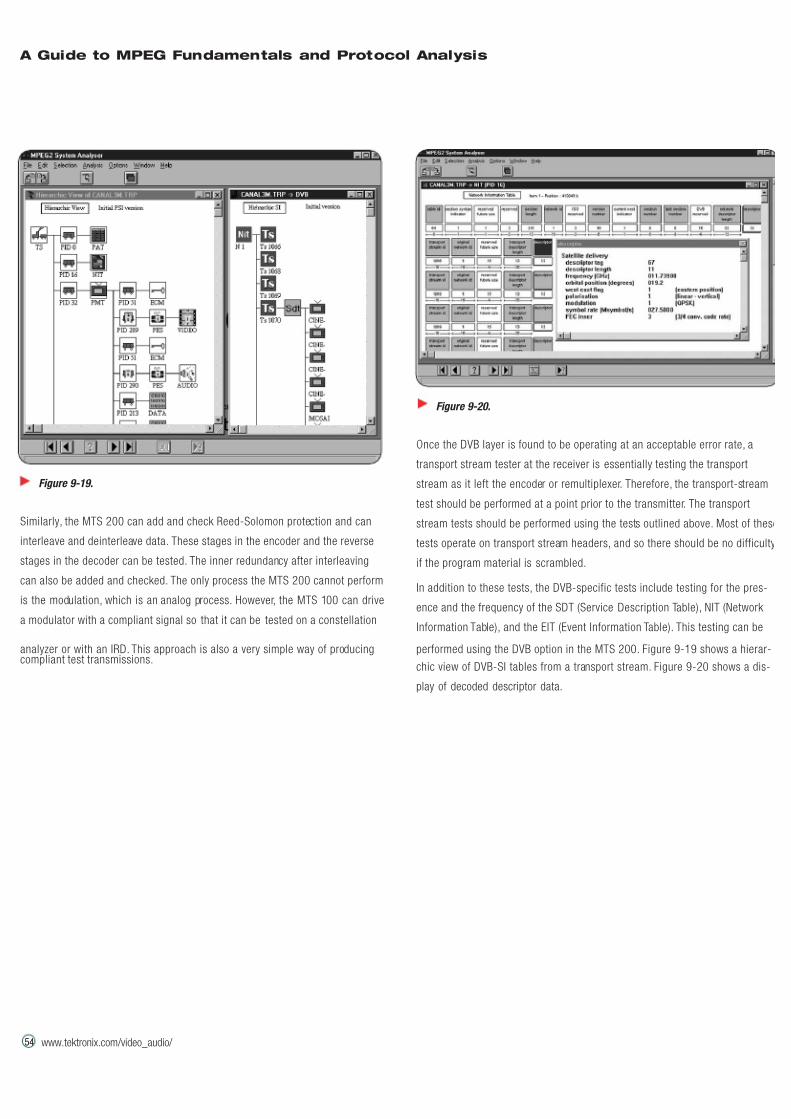
7/16/2019 MPEG Tektronix
http://slidepdf.com/reader/full/mpeg-tektronix 60/64
54
A Guide to MPEG Fundamentals and Protocol Analysis
www.tektronix.com/video_audio/ 54
Similarly, the MTS 200 can add and check Reed-Solomon protection and can
interleave and deinterleave data. These stages in the encoder and the reverse
stages in the decoder can be tested. The inner redundancy after interleaving
can also be added and checked. The only process the MTS 200 cannot perform
is the modulation, which is an analog process. However, the MTS 100 can drive
a modulator with a compliant signal so that it can be tested on a constellation
analyzer or with an IRD. This approach is also a very simple way of producingcompliant test transmissions.
Once the DVB layer is found to be operating at an acceptable error rate, a
transport stream tester at the receiver is essentially testing the transport
stream as it left the encoder or remultiplexer. Therefore, the transport-stream
test should be performed at a point prior to the transmitter. The transport
stream tests should be performed using the tests outlined above. Most of these
tests operate on transport stream headers, and so there should be no difficulty
if the program material is scrambled.
In addition to these tests, the DVB-specific tests include testing for the pres-
ence and the frequency of the SDT (Service Description Table), NIT (Network
Information Table), and the EIT (Event Information Table). This testing can be
performed using the DVB option in the MTS 200. Figure 9-19 shows a hierar-
chic view of DVB-SI tables from a transport stream. Figure 9-20 shows a dis-
play of decoded descriptor data.
Figure 9-19.
Figure 9-20.
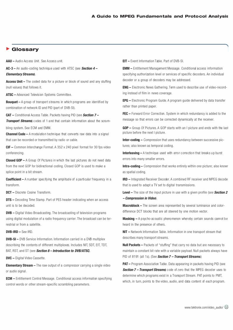
7/16/2019 MPEG Tektronix
http://slidepdf.com/reader/full/mpeg-tektronix 61/64
A Guide to MPEG Fundamentals and Protocol Analysis
www.tektronix.com/video_audio/ 55
AAU – Audi o Access Unit . See Access unit.
AC-3 – An audio -cod ing technique used with ATSC (see Section 4 –
Elementary Streams ).
Access Unit – The coded data for a picture or block of sound and any stuffing
(null values) that follows it.
ATSC – Advanced Televis ion Systems Committee.
Bouquet – A g roup of transpor t s treams in which programs are iden tifi ed by
combination of network ID and PID (part of DVB-SI).
CAT – Conditional Access Table. Packets having PID (see Section 7 –
Transport Streams ) codes of 1 and that contain info rmat ion about the scram-
bling system. See ECM and EMM.
Channel Code – A modulation techn ique that converts raw data into a s igna l
that can be recorded or transmitted by radio or cable.
CIF – Common Interchange Format. A 352 x 240 pixel format for 30 fps video
conferencing.
Closed GOP – A Group Of Pic tures i n which the last pict ures do not need data
from the next GOP for bidirectional coding. Closed GOP is used to make a
splice point in a bit stream.
Coefficient – A number specify ing the ampl itude of a parti cula r f requency in a
transform.
DCT – Discrete Cosine Transform.
DTS – Decoding Time Stamp. Part of PES header indicating when an access
unit is to be decoded.
DVB – Digital Video Broadcasting. The broadcasting of television programs
using digital modulation of a radio frequency carrier. The broadcast can be ter-
restrial or from a satellite.
DVB-IRD – See IRD.
DVB-SI – DVB Service Information. Information carried in a DVB multiplex
describing the contents of different multiplexes. Includes NIT, SDT, EIT, TDT,
BAT, RST, and ST (see Section 8 – Introduction to DVB/ATSC ).
DVC – Digital Video Cassette.
Elementary Stream – The raw output of a compressor carrying a single video
or audio signal.
ECM – Entitlement Control Message. Conditional access information specifying
control words or other stream-specific scrambling parameters.
EIT – Event Information Table. Part of DVB-SI.
EMM – Entitlement Management Message. Conditional access information
specifying authorization level or services of specific decoders. An individual
decoder or a group of decoders may be addressed.
ENG – Electronic News Gathering. Term used to describe use of video-record-
ing instead of film in news coverage.
EPG – Electronic Program Guide. A program guide delivered by data transfer
rather than printed paper.
FEC – Forward Error Correction. System in which redundancy is added to the
message so that errors can be corrected dynamically at the receiver.
GOP – Group Of Pictures. A GOP starts with an I picture and ends with the last
picture before the next I picture.
Inter-coding – Compression that uses redundancy between successive pic-
tures; also known as temporal coding.
Interleaving – A techn ique used with erro r correction that breaks up bu rst
errors into many smaller errors.
Intra-coding – Compression that works entirely within one picture; also known
as spatial coding.
IRD – Integrated Receiver Decoder. A combined RF receiver and MPEG decoder
that is used to adapt a TV set to digital transmissions.
Level – The size of the input picture in use with a given profile (see Section 2
– Compression in Video ).
Macroblock – The screen area represented by several luminance and color-
difference DCT blocks that are all steered by one motion vector.
Masking – A psycho-acoust ic phenomenon whereby certain sounds cannot be
heard in the presence of others.
NIT – Network Information Table. Information in one transport stream that
describes many transport streams.
Null Packets – Packets of “stuffing” that carry no data but are necessary to
maintain a constant bit rate with a variable payload. Null packets always have
PID of 8191 (all 1s). (See Section 7 – Transport Streams .)
PAT – Program Association Table. Data appearing in packets having PID (see
Section 7 – Transport Streams ) code of z ero that the MPEG decoder uses to
determine which programs exist in a Transport Stream. PAT points to PMT,
which, in turn, points to the video, audio, and data content of each program.
Glossary
7/16/2019 MPEG Tektronix
http://slidepdf.com/reader/full/mpeg-tektronix 62/64
56
A Guide to MPEG Fundamentals and Protocol Analysis
www.tektronix.com/video_audio/ 565656
PCM – Pulse Code Modulation. A technical term for an analog source wave-
form, for example, audio or video signals, expressed as periodic, numerical
samples. PCM is an uncompressed digital signal.
PCR – Program Clock Reference. The sample of the encoder clock count that is
sent in the program header to synchronize the decoder clock.
PCRI – Interpolated Program Clock Reference. A PCR estimated from a previ-
ous PCR and used to measure jitter.
PID – Program Identifier. A 13-bit code in the transport packet header. PID 0
indicates that the packet contains a PAT PID. (See Section 7 – Transport
Streams .) PID 1 indicates a packet that contains CAT. The PID 8191 (all 1s)
indicates null (stuffing) packets. All packets belonging to the same elementary
stream have the same PID.
PMT – Program Map Tables. The tables in PAT that point to video, audio, and
data content of a transport stream.
Packets – A term used in two contexts : in program streams, a packet is a unit
that contains one or more presentation units; in transport streams, a packet is
a small, fixed-size data quantum.
Preprocessing – The video signal processing that occurs before MPEG
Encoding. Noise reduction, downsampling, cut-edit identification, and 3:2 pull-
down identification are examples of preprocessing.
Profile – Specifies the coding syntax used.
Program Stream – A b it stream containi ng compressed v ideo , audio, and tim-
ing information.
PTS – Presentation Time Stamps. The time at which a presentation unit is to be
available to the viewer.
PSI – Program Specific Information. Information that keeps track of the differ-
ent programs in an MPEG transport stream and in the elementary streams in
each program. PSI includes PAT, PMT, NIT, CAT, ECM, and EMM.
PSI/SI – A general term for combined MPEG PSI and DVB-SI.
PU – Presentation Unit. One compressed picture or block of audio.
QCIF – One-quarter-resolution (176 x 144 pixels) Common Interchange Format.
See CIF.
QSIF – One-quarter-resolution Source Input Format. See SIF.
RLC – Run Length Coding. A coding scheme that counts number of similar bits
instead of sending them individually.
SDI – Serial Digital Interface. Serial coaxial cable interface standard intended
for production digital video signals.
STC – System Time Clock. The common clock used to encode video and audio
in the same program.
SDT – Service Description Table. A table listing the providers of each service in
a transport stream.
SI – See DVB-SI.
SIF – Source Input Format. A half-resolution input signal used by MPEG-1.
ST – Stuffing Table.
Scalability – A character ist ic of MPEG-2 t hat prov ides for mult iple qual ity lev-
els by providing layers of video data. Multiple layers of data allow a complex
decoder to produce a better picture by using more layers of data, while a more
simple decoder can still produce a picture using only the first layer of data.
Stuffing – Meaningless data added to maintain constant bit rate.
Syndrome – Initial result of an error checking calculation. Generally, if the syn
drome is zero, there is assumed to be no error.
TDAC – Time Domain Aliasing Cancellation. A coding technique used in AC-3
audio compression.
TDT – Time and Date Table. Used in DVB-SI.
T-STD – Transport Stream System Target Decoder. A decoder having a certain
amount of buffer memory assumed to be present by an encoder.
Transport Stream – A multi plex of several program streams that are carr ied in
packets. Demultiplexing is achieved by different packet IDs (PIDs). See PSI,
PAT, PMT, and PCR.
Truncation – Shortening the wordlength of a sample or coefficient by removing
low-order bits.
VAU – Video Access Unit. One compressed picture in program stream.
VLC – Variable Length Coding. A compressed technique that allocates short
codes to frequency values and long codes to infrequent values.
VOD – Video On Demand. A system in which television programs or movies are
transmitted to a single consumer only when requested.
Vector – A motion compensati on parame ter that tell s a decoder how to shif t
part of a previous picture to more closely approximate the current picture.
Wavelet – A t ransform in the basi s f unct ion that is not of fixed l ength bu t thatgrows longer as frequency reduces.
Weighting – A method of chang ing the dist ribution of the noise that is due to
truncation by pre-multiplying values.

7/16/2019 MPEG Tektronix
http://slidepdf.com/reader/full/mpeg-tektronix 63/64

7/16/2019 MPEG Tektronix
http://slidepdf.com/reader/full/mpeg-tektronix 64/64
www.tektronix.com/video_audio/
ASEAN Countries (65) 356-3900
Australia & New Zealand 61 (2) 9888-0100
Austria, Central Eastern Europe,
Greece, Turkey, Malta & Cyprus +43 2236 8092 0
Belgium +32 (2) 715 89 70
Brazil and South America 55 (11) 3741-8360
Canada 1 (800) 661-5625
Denmark +45 (44) 850 700
Finland +358 (9) 4783 400
France & North Africa +33 1 69 86 81 81
Germany + 49 (221) 94 77 400
Hong Kong (852) 2585-6688
India (91) 80-2275577
Italy +39 (2) 25086 501
Japan (Sony/Tektronix Corporation) 81 (3) 3448-3111
Mexico, Central America, & Caribbean 52 (5) 666-6333
The Netherlands +31 23 56 95555
Norway +47 22 07 07 00
People’s Republic of China 86 (10) 6235 1230
Republic of Korea 82 (2) 528-5299
South Africa (27 11) 651-5222
Spain & Portugal +34 91 372 6000
Sweden +46 8 477 65 00
Switzerland +41 (41) 729 36 40
Taiwan 886 (2) 2722-9622
United Kingdom & Eire +44 (0)1344 392000
USA 1 (800) 426-2200
For other areas, contact: Tektronix, Inc. at 1 (503) 627-1924
For Further Information
Tektronix maintains a comprehensive, constantly expanding collection of
application notes, technical briefs, and other resources to help engineers
working on the cutting edge of technology.
Please visit “Resources For You” on our Web site at www.tektronix.com